Comparison of Bayesian predictive methods formodel selection

Juho Piironen∗ and Aki Vehtari∗

Abstract.

The goal of this paper is to compare several widely used Bayesian model selec-tion methods in practical model selection problems, highlight their differences andgive recommendations about the preferred approaches. We focus on the variablesubset selection for regression and classification and perform several numericalexperiments using both simulated and real world data. The results show that theoptimization of a utility estimate such as the cross-validation score is liable tofinding overfitted models due to relatively high variance in the utility estimateswhen the data is scarce. Better and much less varying results are obtained byincorporating all the uncertainties into a full encompassing model and projectingthis information onto the submodels. The reference model projection appears tooutperform also the maximum a posteriori model and the selection of the mostprobable variables. The study also demonstrates that the model selection cangreatly benefit from using cross-validation outside the searching process both forguiding the model size selection and assessing the predictive performance of thefinally selected model.

Keywords: Bayesian model selection, cross-validation, WAIC, MAP, Medianprobability model, reference model, projection, overfitting, selection bias.

1 Introduction

Model selection is one of the fundamental problems in statistical modeling. The oftenadopted view for model selection is not to identify the true underlying model but ratherto find a model which is useful. Typically the usefulness of a model is measured by itsability to make predictions about future or yet unseen observations. Even though theprediction would not be the most important part concerning the modelling problemat hand, the predictive ability is still a natural measure for figuring out whether themodel makes sense or not. If the model gives poor predictions, there is not much pointin trying to interpret the model parameters. We refer to the model selection based onassessing the predictive ability of the candidate models as predictive model selection.

Numerous methods for Bayesian predictive model selection and assessment havebeen proposed and the various approaches and their theoretical properties have beenextensively reviewed by Vehtari and Ojanen (2012). This paper is a follow-up to theirwork. The review of Vehtari and Ojanen (2012) being qualitative, our contribution isto compare many of the different methods quantitatively in practical model selectionproblems, discuss the differences, and give recommendations about the preferred ap-proaches. We believe this study will give useful insights because the comparisons to the

∗Aalto University, Finland juho.piironen@aalto.fi aki.vehtari@aalto.fi

arX

iv:1

503.

0865

0v1

[st

at.M

E]

30

Mar

201

5

2 Bayesian model selection methods

existing techniques are often inadequate in the original articles presenting new methods.Our experiments will focus on variable subset selection on linear models for regressionand classification, but the discussion is general and the concepts apply also to othermodel selection problems.

A fairly popular method in Bayesian literature is to select the maximum a posteriori(MAP) model which, in the case of a uniform prior on the model space, reduces tomaximizing the marginal likelihood and the model selection can be performed usingBayes factors (e.g. Kass and Raftery, 1995; Han and Carlin, 2001). In the input variableselection context, also the marginal probabilities of the variables have been used (e.g.Brown et al., 1998; Barbieri and Berger, 2004; Narisetty and He, 2014). Another commonapproach is to choose the model based on its estimated predictive ability, preferably byusing Bayesian leave-one-out cross-validation (LOO-CV) (Geisser and Eddy, 1979) orthe widely applicable information criterion (WAIC) (Watanabe, 2009) both of whichare known to give a nearly unbiased estimate of the predictive ability of a given model(Watanabe, 2010). Also several other predictive criteria with different loss functions havebeen proposed, for instance the deviance information criterion (DIC) by Spiegelhalteret al. (2002) and the various squared error measures by Laud and Ibrahim (1995),Gelfand and Ghosh (1998), and Marriott et al. (2001) none of which, however, areunbiased estimates of the true generalization utility of the model.

An alternative approach is to construct a full encompassing reference model whichis believed to best represent the uncertainties regarding the modelling task and choosea simpler submodel that gives nearly similar predictions as the reference model. Thisapproach was pioneered by Lindley (1968) who considered input variable selection forlinear regression and used the model with all the variables as the reference model. Theidea was extended by Brown et al. (1999, 2002). A related method is due to San Martiniand Spezzaferri (1984) who used the Bayesian model averaging solution as the referencemodel and Kullback–Leibler divergence for measuring the difference between the predic-tions of the reference model and the candidate model instead of the squared error lossused by Lindley. Another related method is the reference model projection by Goutisand Robert (1998) and Dupuis and Robert (2003) in which the information containedin the posterior of the reference model is projected onto the candidate models.

Although LOO-CV and WAIC can be used to obtain a nearly unbiased estimate ofthe predictive ability of a given model, both of these estimates contain a stochastic errorterm whose variance can be substantial when the dataset is not very large. This variancein the estimate may lead to overfitting in the selection process causing nonoptimalmodel selection and inducing bias in the performance estimate for the selected model(e.g. Varma and Simon, 2006; Cawley and Talbot, 2010). The overfitting in the selectionmay be negligible if only a few models are being compared but, as we will demonstrate,may become a significant problem for a larger number of candidate models, such as invariable selection.

Our results show that the optimization of CV or WAIC may yield highly varyingresults and lead to selecting a model with predictive performance far from optimal. Theselection of the most probable inputs or the MAP model tends to reduce the variabilityleading to better selection. However, the results also show that the reference model based

J. Piironen and A. Vehtari 3

selection, especially the projection approach, typically gives even better and less varyingresults. This is due to significantly reduced variance in the performance evaluation forthe candidate models.

Despite its advantages, the reference model approach has suffered from difficulty indeciding how many variables should be selected in order to get predictions close to thereference model (Peltola et al., 2014; Robert, 2014). Our study will demonstrate thatthe model selection can highly benefit from using cross-validation outside the variablesearching process both for guiding the model size selection and assessing the predictiveperformance of the finally selected model.

The paper is organized as follows. In Section 2 we shortly go through the modelselection methods discussed in this paper. Section 3 discusses and illustrates the over-fitting in model selection and the consequent selection induced bias in the performanceevaluation of the chosen model. Section 4 is devoted to the numerical experiments andforms the core of the paper. The discussion in Section 5 concludes the paper.

2 Approaches for Bayesian model selection

This section discusses shortly the proposed methods for Bayesian model selection rele-vant for this paper. We do not attempt anything close to a comprehensive review butsummarize the methods under comparison. See the review by Vehtari and Ojanen (2012)for a more complete discussion.

The section is organized as follows. Section 2.1 discusses how the predictive abilityof a model is defined in terms of an expected utility and Sections 2.2–2.5 shortly reviewthe methods. Following Bernardo and Smith (1994) and Vehtari and Ojanen (2012) wehave categorized the methods into M-closed, M-completed, and M-open views, seeTable 1. M-closed means assuming that one of the candidate models is the true datagenerating model. Under this assumption, one can set prior probabilities for each modeland form the Bayesian model averaging solution (see Section 2.5). The M-completedview abandons the idea of a true model, but still forms a reference model which isbelieved to be the best available description of the future observations. In the M-openview one does not assume one of the models being true and also rejects the idea ofconstructing the reference model.

Throughout Section 2, the notation assumes a model M which predicts an outputy given an input variable x. The same notation is used both for scalars and vectors.We denote the future observations by y and the model parameters by θ. To make thenotation simpler, we denote the training data as D = {(xi, yi)}ni=1.

2.1 Predictive ability as an expected utility

The predictive performance of a model is typically defined in terms of a utility functionthat describes the quality of the predictions. An often used utility function measuringthe quality of the predictive distribution of the candidate model Mk is the logarithmic

4 Bayesian model selection methods

Table 1: Categorization of the different model selection methods discussed in this paper.

View Methods

Section 2.2 Generalization utility estimation(M-open view)

Cross-validation, WAIC, DIC

Section 2.3 Self/posterior predictive criteria(Mixed view)

L2-, L2cv- and L2

k-criteria

Section 2.4 Reference model approach(M-completed view)

Reference predictive method,Projection predictive method

Section 2.5 Model space approach(M-closed view)

Maximum a posteriori model,Median model

score (Good, 1952)

u(Mk, y) = log p(y |D,Mk) . (1)

Here we have left out the future input variables x to simplify the notation. The logarith-mic score is a widely accepted utility function due to its information theoretic groundsand will be used in this paper. However, we point out that in principle any other utilityfunction could be considered, and the choice of a suitable utility function might also beapplication specific.

Since the future observations y are unknown, the utility function u(Mk, y) can notbe evaluated beforehand. Therefore one usually works with the expected utilities instead

u(Mk) = E [log p(y |D,Mk)] =

∫pt(y) log p(y |D,Mk)dy, (2)

where pt(y) denotes the true data generating distribution. This expression will be re-ferred to as the generalization utility or more loosely as the predictive performance ofmodel Mk. Maximizing (2) is equivalent to minimizing the Kullback–Leibler (KL) di-vergence from the true data generating distribution pt(y) to the predictive distributionof the candidate model Mk.

2.2 Generalization utility estimation

Cross-validation

The generalization utility (2) can be estimated by using the already obtained sampleD as proxy for the true data generating distribution pt(y). However, estimating theexpected utility using the same data D that were used to train the model leads to anoptimistic estimate of the generalization performance. A better estimate is obtainedby dividing the data into k subsets and using each of these sets in turn for validationwhile training the model using the remaining k− 1 sets. This gives the Bayesian k-fold

J. Piironen and A. Vehtari 5

cross-validation (CV) utility (Geisser and Eddy, 1979)

k-fold-CV =1

n

n∑i=1

log p(yi |xi, D\s(i),Mk), (3)

where s(i) denotes the validation set that contains the ith point and D\s(i) the trainingdata from which this subset has been removed. Conditioning the predictions on fewerthan n data points introduces bias in the utility estimate. This bias can be corrected(Burman, 1989) but small k increases the variance in the estimate. One would prefer toset k = n computing the leave-one-out utility (LOO-CV) but without any computationalshortcuts this is often computationally infeasible as the model would need to be fittedn times. An often used compromise is k = 10. Analytical approximations for LOO arediscussed by Vehtari et al. (2014) and computations using posterior samples by Vehtariand Gelman (2014).

Information criteria

Information criteria offer a computationally appealing way of estimating the general-ization performance of the model. A fully Bayesian criterion is the widely applicableinformation criterion (WAIC) by Watanabe (2009, 2010). WAIC can be calculated as

WAIC =1

n

n∑i=1

log p(yi |xi, D,Mk)− V

n, (4)

where the first term is the training utility and V is the functional variance given by

V =

n∑i=1

{E[(log p(yi |xi, θ,Mk))2

]− E [log p(yi |xi, θ,Mk)]

2}. (5)

Here both of the expectations are taken over the posterior p(θ |D,Mk). Watanabe (2010)proved that WAIC is asymptotically equal to the Bayesian LOO-CV and to the gen-eralization utility (2), and the error is o(1/n). Watanabe’s proof gives Bayesian LOOand WAIC a solid theoretical justification in the sense that they measure the predictiveability of the model including the uncertainty in the parameters and can be used alsofor singular models (the set of the “true parameters” consists of more than one point).

Another still popular method is the deviance information criterion (DIC) proposedby Spiegelhalter et al. (2002). DIC estimates the generalization performance of the modelwith parameters fixed to the posterior mean θ = E [θ |D,Mk]. DIC can be written as

DIC =1

n

n∑i=1

log p(yi |xi, θ,Mk)− peff

n, (6)

where peff is the effective number of parameters which can be estimated as

peff = 2

n∑i=1

(log p(yi |xi, θ,Mk)− E [log p(yi |xi, θ,Mk)]

), (7)

6 Bayesian model selection methods

where the expectation is taken over the posterior. From Bayesian perspective, DIC isnot theoretically justified since it measures the fit of the model when the parameters arefixed to the posterior expectation and is not therefore an unbiased estimate of the truegeneralization utility (2). The use of a point estimate is questionable not only becauseof Bayesian principles, but also from a practical point of view especially when the modelis singular.

2.3 Mixed self and posterior predictive criteria

There exists a few criteria that are not unbiased estimates of the true generalizationutility (2) but have been proposed for model selection. These criteria do not fit tothe M-open view since the candidate models are partially assessed based on their ownpredictive properties and therefore these criteria resembleM-closed/M-completed view(see Vehtari and Ojanen, 2012).

Laud and Ibrahim (1995) proposed a selection criterion for regression derived byconsidering replicated measurements y at the training inputs. The criterion measuresthe expected squared error between the new observations and the old ones y over theposterior predictive distribution of the candidate model Mk. The error measure can bedecomposed as

L2 =

n∑i=1

(yi − E [y |xi, D,Mk])2 +

n∑i=1

Var [y |xi, D,Mk] , (8)

that is, as a sum of the squared errors for mean predictions plus sum of the predictivevariances. The preferred model is then the one which minimizes (8).

Marriott et al. (2001) proposed a closely related criterion which is a cross-validatedversion of (8)

L2cv =

n∑i=1

(yi − E[y |xi, D\s(i),Mk

])2 +

n∑i=1

Var[y |xi, D\s(i),Mk

]. (9)

This sounds intuitively better than the L2-criterion because it does not use the samedata for training and testing. However, relatively high variance in the error estimatemay cause significant overfitting in model selection as discussed in Section 3 and demon-strated experimentally in Section 4.

Yet another related criterion based on a replicated measurement was proposed byGelfand and Ghosh (1998). The authors considered an optimal point prediction whichis designed to be close to both the observed and future data and the relative importancebetween the two is adjusted by a free parameter k. Omitting the derivation, the lossfunction becomes

L2k =

k

k + 1

n∑i=1

(yi − E [y |xi, D,Mk])2 +

n∑i=1

Var [y |xi, D,Mk] . (10)

J. Piironen and A. Vehtari 7

When k →∞, this is the same as the L2-criterion (8). On the other hand, when k = 0,the criterion reduces to the sum of the predictive variances, and the model with thenarrowest predictive distribution is chosen. In their experiment, the authors reportedthat the results were not very sensitive to the choice of k.

2.4 Reference model approach

Section 2.2 reviewed methods for utility estimation that are based on sample reusewithout any assumptions on the true model (M-open view). An alternative way is toconstruct a reference model, which is believed to best describe our knowledge about thefuture observations, and perform the utility estimation almost as if it was the true datagenerating distribution (M-completed view). We refer to this as the reference modelapproach. There are basically two somewhat different but related approaches that fitinto this category, namely the reference and projection predictive methods which willbe discussed separately.

Reference predictive method

Assuming we have constructed a reference model which we believe best describes ourknowledge about the future observations, the utilities of the candidate models Mk canbe estimated by replacing the true distribution pt(y) in (2) by the predictive distributionof the reference model p(y |D,M∗). Averaging this over the training inputs {xi}ni=1 givesthe reference utility

uref =1

n

n∑i=1

∫p(y |xi, D,M∗) log p(y |xi, D,Mk)dy . (11)

As the reference model is in practice different from the true data generating model,the reference utility is a biased estimate of the true generalization utility (2). Themaximization of the reference utility is equivalent to minimizing the predictive KL-divergence between the reference model M∗ and the candicate model Mk at the traininginputs

δ(M∗‖Mk) =1

n

n∑i=1

KL (p(y |xi, D,M∗) ‖ p(y |xi, D,Mk)) . (12)

The model choice can then be based on the strict minimization of the discrepancy mea-sure (12), or choosing the simplest model that has an acceptable discrepancy. What ismeant by “acceptable” may be somewhat arbitrary and context dependent. For morediscussion, see the concept of relative explanatory power in the next section, Equa-tion (16).

The reference predictive approach is inherently a less straightforward approach tomodel selection than the methods presented in Section 2.2, because it requires the con-struction of the reference model and it is not obvious how it should be done. San Martiniand Spezzaferri (1984) proposed using the Bayesian model average (19) as the reference

8 Bayesian model selection methods

model (see Sec. 2.5). In the variable selection context, the model averaging correspondsto a spike-and-slab type prior (Mitchell and Beauchamp, 1988) which has been exten-sively used for linear models (see, e.g., George and McCulloch, 1993, 1997; Raftery et al.,1997; Brown et al., 2002; Lee et al., 2003; O’Hara and Sillanpaa, 2009; Narisetty andHe, 2014) and extended and applied to regression for over one million variables (Peltolaet al., 2012a,b). However, we emphasize that any other model or prior could be usedas long as we believe it reflects our best knowledge of the problem and allows conve-nient computation. For instance the Horseshoe prior (Carvalho et al., 2009, 2010) hasbeen demonstated to have desirable properties empirically and theoretically assuminga properly chosen shrinkage factor (Datta and Ghosh, 2013; van der Pas et al., 2014).

Projection predictive method

A related but somewhat different alternative to the reference predictive method (pre-vious section) is the projection approach. The idea is to project the information in theposterior of the reference model M∗ onto the candidate models so that the predictivedistribution of the candidate model remains as close to the reference model as possible.Thus the key aspect is that the candidate models are trained by the fit of the referencemodel, not by the data. Therefore also the prior needs to be specified only for the ref-erence model. The idea behind the projection is quite generic and Vehtari and Ojanen(2012) discuss the general framework in more detail.

A practical means for doing the projection was proposed by Goutis and Robert(1998) and further discussed by Dupuis and Robert (2003). Given the parameter of thereference model θ∗, the projected parameter θ⊥ in the parameter space of model Mk isdefined via

θ⊥ = arg minθ

1

n

n∑i=1

KL (p(y |xi, θ∗,M∗) ‖ p(y |xi, θ,Mk)) . (13)

The discrepancy between the reference model M∗ and the candidate model Mk is thendefined to be the expectation of the divergence over the posterior of the reference model

δ(M∗‖Mk) =1

n

n∑i=1

Eθ∗|D,M∗

[KL(p(y |xi, θ∗,M∗) ‖ p(y |xi, θ⊥,Mk)

)]. (14)

The posterior expectation in (14) is in general not available analytically. Dupuis andRobert (2003) proposed calculating the discrepancy by drawing samples {θ∗s}Ss=1 fromthe posterior of the reference model, calculating the projected parameters {θ⊥s }Ss=1 in-dividually according to (13), and then approximating (14) as

δ(M∗‖Mk) ≈ 1

nS

n∑i=1

S∑s=1

KL(p(y | xi, θ∗s ,M∗) ‖ p(y | xi, θ⊥s ,Mk)

). (15)

Moreover, Dupuis and Robert (2003) introduced a measure called relative explanatorypower

φ(Mk) = 1− δ(M∗‖Mk)

δ(M∗‖M0), (16)

J. Piironen and A. Vehtari 9

where M0 denotes the empty model, that is, the model that has the largest discrepancyto the reference model. In terms of variable selection, M0 is the variable free model. Bydefinition, the relative explanatory power obtains values between 0 and 1, and Dupuisand Robert (2003) proposed choosing the simplest model with enough explanatorypower, for example 90%, but did not discuss the effect of this threshold for the predictiveperformance of the selected models. We note that, in general, the relative explanatorypower is an unreliable indicator of the predictive performance of the submodel. This isbecause the reference model is typically different from the true data generating modelMt, and therefore both M∗ and Mk may have the same discrepancy to Mt (that is,the same predictive ability) although the discrepancy between M∗ and Mk would benonzero.

Peltola et al. (2014) proposed an alternative way of deciding a suitable model sizebased on cross-validation outside the searching process. In other words, in a k-foldsetting the searching is repeated k times each time leaving 1/k of the data for testing,and the performance of the found models are tested on this left-out data. Note thatalso the reference model is trained k times and each time its performance is evaluatedon the left-out data. Thus, one can compare the utility of both the found models andthe reference model on the independent data and estimate, for instance, how manyvariables are needed to get statistically indistinguishable predictions compared to thereference model. More precisely, if um denotes the estimated expected utility of choosingm variables and u∗ denotes the estimated utility for the reference model, the modelscan be compared by estimating the probability

Pr [u∗ − um ≤ ∆u] , (17)

that is, the probability that the utility difference compared to the reference model isless than ∆u ≥ 0. Peltola et al. (2014) suggested estimating the probabilities aboveby using Bayesian bootstrap (Rubin, 1981) and reported results for all model sizes for∆u = 0.

The obvious drawback in this approach is the increased computations (as the selec-tion and reference model fitting is repeated k times), but in Section 4.3 we demonstratethat this approach may be very useful when investigating how the predictive abilitybehaves as a function of the number of variables.

2.5 Model space approach

Bayesian formalism has a natural way of describing the uncertainty with respect to theused model specification given an exhaustive list of candidate models {Mk}Kk=1. Thedistribution over the model space is given by

p(M |D) ∝ p(D |M) p(M) . (18)

The predictions are then obtained from the Bayesian model averaging (BMA) solution

p(y |D) =

K∑k=1

p(y |D,Mk) p(Mk |D) . (19)

10 Bayesian model selection methods

Strictly speaking, forming the model average means adopting the M-closed view, that

is, assuming one of the candidate models is the true data generating model. In practice,

however, averaging over the discrete model space does not differ in any sense from in-

tegrating over the continuous parameters which is the standard procedure in Bayesian

modeling. Moreover, BMA has been shown to have a good predictive performance both

theoretically and empirically (Raftery and Zheng, 2003) and especially in variable selec-

tion context the integration over the different variable combinations is widely accepted.

See the review by Hoeting et al. (1999) for a thorough discussion of Bayesian model

averaging.

From a model selection point of view, one may choose the model maximizing (18)

ending up with the maximum a posteriori (MAP) model. Assuming the true data gen-

erating model belongs to the set of the candidate models, MAP model can be shown

to be the optimal choice under the zero-one utility function (utility being one if the

true model is found, and zero otherwise). If the models are given equal prior probabili-

ties, p(M) ∝ 1, finding the MAP model reduces to maximizing the marginal likelihood

p(M |D) ∝ p(D |M), also referred to as the type-II maximum likelihood.

Barbieri and Berger (2004) proposed a related variable selection method for the

Gaussian linear model and named it the Median probability model (which we abbreviate

simply as the Median model). The Median model is defined as the model containing

all the variables with marginal posterior probability greater than 12 . Let binary vector

γ = (γ1, . . . , γp) denote which of the variables are included in the model (γj = 1 meaning

that variable j is included). The marginal posterior inclusion probability of variable j

is then

πj =∑

Mk : γj=1

p(Mk |D), (20)

that is, the sum of the posterior probabilities of the models which include variable j.

The Median model γmed is then defined componentwise as

γjmed =

{1, if πj ≥ 1

2 ,

0, otherwise .(21)

The authors showed that when the predictors are orthogonal, that is when Q = E[xxT

]is diagonal, the Median model is the optimal choice. By optimal the authors mean

the model whose predictions for future y are closest to the Bayesian model averaging

prediction (19) in the squared error sense. The authors admit that the assumption of

the orthogonal predictors is a strong condition that does not often apply. The Median

model also assumes that the optimality is defined in terms of the mean predictions,

meaning that the uncertainty in the predictive distributions is ignored. Moreover, the

Median model is derived assuming Gaussian noise and thus the theory does not apply,

for instance, to classification problems.

J. Piironen and A. Vehtari 11

3 Overfitting and selection induced bias

As discussed in Section 2.1, the performance of a model is usually defined in terms of theexpected utility (2). Many of the proposed selection criteria rewieved in Sections 2.2–2.5 can be thought of as estimates of this quantity even if not designed directly for thispurpose.

Consider a hypothetical utility estimation method. For a fixed training dataset D,its utility estimate gk = g(Mk, D) for model Mk can be decomposed as

gk = uk + ek, (22)

where uk = u(Mk, D) represents the true generalization utility of the model, and ek =e(Mk, D) is the error in the utility estimate. Note that also uk depends on the observeddataset D, because favourable datasets lead to better generalization performance. Ifthe utility estimate is correct on average over the different datasets ED [gk] = ED [uk]or equivalently ED [ek] = 0, we say the estimate g is unbiased, otherwise it is biased.The unbiasedness of the utility estimate is often considered as beneficial for modelselection. However, the unbiasedness is intrinsically unimportant for model selection,and a successful model selection does not necessarily require unbiased utility estimates.To see this, note that the only requirement for a perfect model selection criterion is thatthe higher utility estimate implies higher generalization performance, that is gk > g`implies uk > u` for all models Mk and M`. This condition can be satisfied even ifED [gk] 6= ED [uk].

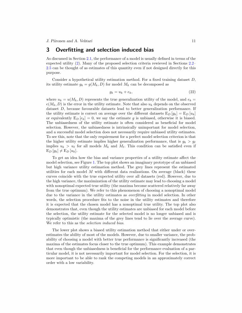
To get an idea how the bias and variance properties of a utility estimate affect themodel selection, see Figure 1. The top plot shows an imaginary prototype of an unbiasedbut high variance utility estimation method. The grey lines represent the estimatedutilities for each model M with different data realizations. On average (black) thesecurves coincide with the true expected utility over all datasets (red). However, due tothe high variance, the maximization of the utility estimate may lead to choosing a modelwith nonoptimal expected true utility (the maxima become scattered relatively far awayfrom the true optimum). We refer to this phenomenon of choosing a nonoptimal modeldue to the variance in the utility estimates as overfitting in model selection. In otherwords, the selection procedure fits to the noise in the utility estimates and thereforeit is expected that the chosen model has a nonoptimal true utility. The top plot alsodemonstrates that, even though the utility estimates are unbiased for each model beforethe selection, the utility estimate for the selected model is no longer unbiased and istypically optimistic (the maxima of the grey lines tend to lie over the average curve).We refer to this as the selection induced bias.

The lower plot shows a biased utility estimation method that either under or over-estimates the ability of most of the models. However, due to smaller variance, the prob-ability of choosing a model with better true performance is significantly increased (themaxima of the estimates focus closer to the true optimum). This example demonstratesthat even though the unbiasedness is beneficial for the performance evaluation of a par-ticular model, it is not necessarily important for model selection. For the selection, it ismore important to be able to rank the competing models in an approximately correctorder with a low variability.

12 Bayesian model selection methods

Unbiased, high variance

Candidate models M

Utility

Biased, low variance

g(M,Di)

ED [g(M,D)]

ED [u(M,D)]

Selected models

Figure 1: Schematic illustration of an unbiased (top) and a biased (bottom) utilityestimation method. Grey lines denote the utility estimates for different datasets Di,black is the average, and red the true expected utility. In this case, the biased method islikely to choose better models (dashed lines) due to better tradeoff in bias and variance.

The overfitting in model selection and the selection induced bias are importantconcepts that have received relatively little attention compared to the vast literatureon model selection in general. However, the topic has been discussed for example byRencher and Pun (1980), Reunanen (2003), Varma and Simon (2006), and Cawley andTalbot (2010). These authors discuss mainly the model selection using cross-validation,but the ideas apply also to other utility estimation methods. As discussed in Section 2.2,cross-validation gives a nearly unbiased estimate of the generalization performance ofany given model, but the selection process may overfit when the variance in the utilityestimates is high (as depicted in the top plot of Figure 1). This will be demonstratedempirically in Section 4. The variance in the utility estimate is different for differentestimation methods but may generally be considerable for small datasets. The proba-bility of fitting to noise increases also with the number of models being compared, andmay become a problem for example in variable selection.

4 Numerical experiments

This section compares the methods presented in Section 2 in practical variable selec-tion problems. Section 4.1 discusses the used models and Sections 4.2 and 4.3 showillustrative examples using simulated and real world data, respectively.

J. Piironen and A. Vehtari 13

4.1 Models

We will consider both regression and binary classification problems. To reduce the com-putational burden involved in the experiments, we consider only linear models. Forregression, we apply the standard Gaussian model

y |x,w, σ2 ∼ N(wTx, σ2

),

w |σ2, τ2 ∼ N(0, τ2σ2I

),

σ2 ∼ Inv-Gamma (ασ, βσ) ,

τ2 ∼ Inv-Gamma (αw, βw) .

(23)

For the binary classification we use the probit model

y |x,w ∼ Ber(Φ(wTx)

),

w | τ2 ∼ N(0, τ2I

),

τ2 ∼ Inv-Gamma (αw, βw) ,

(24)

where Φ(·) denotes the cumulative distribution of the standard normal distribution. Forboth models (23) and (24) we include the intercept term by augmenting a constant termin the input vector x = (1, x1, . . . , xp) and a corresponding term in the weight vectorw = (w0, w1, . . . , wp). For the regression model (23), most of the computations can beobtained analytically because for a given hyperparameter τ2 the prior is conjugate. Theintegration over τ2 can be performed numerically. For the probit model (24) we useMarkov chain Monte Carlo (MCMC) methods to obtain samples from the posterior ofthe weights to get the predictions.

Since we are considering a variable selection problem, the submodels have differentnumber of input variables and therefore different dimensionality for x and w. For nota-tional convenience, the binary vector γ = (γ0, γ1, . . . , γp) denoting which of the variablesare included in the model is omitted in the above formulas. Both in (23) and (24) themodel specification is the same for each submodel γ, only the dimensionality of x andw change. The reference model M∗ is constructed as the Bayesian model average (19)from the submodels using the reversible jump MCMC (RJMCMC) (Green, 1995), whichcorresponds to a spike-and-slab prior for the full model. For the model space we use theprior

γj |π ∼ Ber (π) , j = 1, . . . , p ,

π ∼ Beta (a, b) . (25)

Here parameters a and b adjust the prior beliefs about the number of included variables.For instance when a = 1 and b = 9 the expected number of variables is pE [π] =p a/(a+ b) = p/10. We set γ0 = 1, that is, the intercept term w0 is included in all thesubmodels. The exact values used for the hyperparameters αw, βw, ασ, βσ, a, b will begiven together with the dataset descriptions in Sections 4.2 and 4.3.

14 Bayesian model selection methods

Table 2: Compared model selection methods for the experiments. MAP and Medianmodels are estimated from the RJMCMC samples, for other methods the searchingis done using forward searching (at each step choose the variable that improves theobjective function value the most). The methods are discussed in Section 2.

Abbreviation Method

CV-10 10-fold cross-validation optimization (3)WAIC WAIC optimization (4)DIC DIC optimization (6)L2 L2-criterion optimization (8)L2-CV L2

cv-criterion optimization (9)L2-k L2

k-criterion optimization with k = 1 (10)MAP Maximum a posteriori modelMPP/Median Sort the variables according to their marginal posterior probabilities

(MPP), choose all with probability 0.5 or more (Median) (21)BMA-ref Posterior predictive discrepancy minimization from BMA (12),

choose smallest model having 95% explanatory power (16)BMA-proj Projection of BMA to submodels (15), choose smallest model having

95% explanatory power (16)

4.2 Simulated data

We first introduce a simulated experiment which illustrates a number of importantconcepts and the main differences between the different methods. The data is distributedas follows

x ∼ N (0, R) , R ∈ Rp×p,y |x ∼ N

(wTx, σ2

), σ2 = 1.

We set the total number of variables to p = 100. The variables are divided into groupsof 5 variables. Each variable xj has a zero mean and unit variance and is correlated withother variables in the same group with coefficient ρ but uncorrelated with variables in theother groups (the correlation matrix R is block diagonal). The variables in the first threegroups have weights (w1:5, w6:10, w11:15) = (ξ, 0.5 ξ, 0.25 ξ) while the rest of the variableshave zero weight. Thus there are 15 relevant and 85 irrelevant variables in the data. Theconstant ξ adjusts the signal-to-noise ratio of the data. To get comparable results fordifferent levels of correlation ρ, we set ξ so that σ2/Var [y] = 0.3. For ρ = 0, 0.5, 0.9 thisis satisfied by setting approximately ξ = 0.59, 0.34, 0.28, respectively.

The experiments were carried out varying the training set size n = 100, 200, 400 andthe correlation coefficient ρ = 0, 0.5, 0.9. We used the regression model (23) with priorparameters αw = βw = ασ = βσ = 0.5. As the reference model M∗ we used the Bayesianmodel average with prior a = 1, b = 10. For each combination of (n, ρ) the variableselection was performed with each method listed in Table 2, and then the performance ofthe selected models were tested on an independent test set of size n = 1000. We repeatedthis for 50 different data realizations. As a proxy for the generalization utility (2), we

J. Piironen and A. Vehtari 15

use the test utility, that is, the mean log predictive density (MLPD) on the test set

MLPD(Mk) =1

n

n∑i=1

log p(yi | xi, D,Mk). (26)

To reduce variance over the different data realizations and to better compare the relativeperformance of the different methods, we report the utilities of the selected submodelsMk with respect to the BMA solution M∗

∆MLPD(Mk) = MLPD(Mk)−MLPD(M∗). (27)

On this relative scale zero indicates the same predictive performance as the BMA andnegative values worse.

Figure 2 shows the average number of selected variables and the test utilities ofthe selected models in each data setting with respect to the BMA. For the smallestdataset size many of the methods perform poorly and choose models with bad predictiveperformance, even worse or comparable to the model with no variables at all (the dottedlines). This holds for CV-10, WAIC, DIC, L2, L2-CV, and L2-k, and the conclusioncovers all the levels of correlation between the variables (blue, red and green circles),albeit the high dependency between the variables somewhat improves the results. Theobserved behaviour is due to overfitting in the selection process. Due to scarce data, thehigh variance in the utility estimates leads to selecting overfitted models as discussed inSection 3. These methods perform reasonably only for the largest dataset size n = 400.MAP, Median, BMA-ref, and BMA-proj perform significantly better, choosing smallermodels with predictive ability closer to the BMA. A closer inspection reveals that outof these four, BMA-proj performs best in terms of the predictive ability especially forthe smallest dataset size n = 100, but also chooses more variables than the other threemethods.

To get more insight to the problem, let us examine more closely how the predictiveperformance of the submodels change when variables are selected. Figure 3 shows theCV and test utilities as a function of the number of chosen variables on average forsome of the selection methods for the different training set sizes n. The search pathsfor CV-10 (top row) demonstrate the overfitting in model selection; starting from theempty model and adding variables one at a time one finds models that have high CVutility but much worse test utility. In other words, the performance of the models at thesearch path is dramatically overestimated and the gap between the two curves denotesthe selection induced bias. For the empty model and the model with all the variables theCV utility and the test utility are on average almost the same because these models donot involve any selection. The overfitting in the selection process decreases when the sizeof the training set grows because the variance of the error term in decomposition (22)becomes smaller, but the effect is still visible for n = 400. The behaviour is very similaralso for WAIC, DIC, L2, L2-CV and L2-k (the results for the last three are left out tosave space).

Ordering the variables according to their marginal posterior probabilities (MPP)works much better than CV-10 selecting smaller models with better predictive perfor-mance. However, even more desirable results are obtained by using the reference model

16 Bayesian model selection methods

0 25 50 75 100

n = 200

0 25 50 75 100

n = 100

Variables selected

−1.2 −0.8 −0.4 0

CV-10WAICDICL2L2-CVL2-kMAPMedianBMA-refBMA-proj

∆MLPD(Mk)

−0.6 −0.4 −0.2 0

CV-10WAICDICL2L2-CVL2-kMAPMedianBMA-refBMA-proj

−0.6 −0.4 −0.2 0

CV-10WAICDICL2L2-CVL2-kMAPMedianBMA-refBMA-proj

ρ = 0

ρ = 0.5

ρ = 0.9

0 25 50 75 100

n = 400

Figure 2: Simulated data: Average number of variables chosen (left column) and theaverage test utilities of the chosen models (right column) with 95% credible intervalsfor the different training set sizes n. The utilities are shown with respect to the BMA (27)and the dotted lines denote the performance of the empty model (intercept term only).The colours denote the correlation level between the variables (see the legend). The truenumber of relevant variables is 15 and the results are averaged over 50 data realizations.See Table 2 for the used methods.

approach, especially the projection (BMA-proj). Even for the smallest dataset size, theprojection is able to sort the variables so that a predictive ability very close to the BMAis obtained with about 10–15 variables on average. The results suggest that the projec-tion approach is much less vulnerable to the selection induced bias even though the CVutility is still a biased estimate of the true predictive ability for the chosen models.

Figure 4 shows the variability in the performance of the selected models for thesame selection methods as in Figure 3. The grey lines denote the test utilities for theselected models as a function of number of selected variables for different data realiza-tions and the black line denotes the average (same as in Figure 3). For small trainingset sizes the variability in the predictive performance of the selected submodels is veryhigh for CV-10, WAIC, DIC, and MPP. The reference model approach, especially theprojection, reduces the variability substantially finding submodels with predictive per-formance close to the BMA in all the data realizations. This is another property thatmakes the projection approach more appealing than the other approaches. The results

J. Piironen and A. Vehtari 17

0 25 50 75 100−0.6

−0.3

0

0.3

0 25 50 75 100−0.6

−0.3

0

0.3

n = 200

0 25 50 75 100−0.6

−0.3

0

0.3

CV-10

n = 100

0 25 50 75 100−0.6

−0.3

0

0.3

WAIC

0 25 50 75 100−0.6

−0.3

0

0.3

DIC

0 25 50 75 100−0.6

−0.3

0

0.3

0 25 50 75 100−0.6

−0.3

0

0.3

0 25 50 75 100−0.6

−0.3

0

0.3

0 25 50 75 100−0.6

−0.3

0

0.3

n = 400

0 25 50 75 100−0.6

−0.3

0

0.3

0 25 50 75 100−0.6

−0.3

0

0.3

0 25 50 75 100−0.6

−0.3

0

0.3

MPP

0 25 50 75 100−0.6

−0.3

0

0.3

BMA-ref

0 25 50 75 100−0.6

−0.3

0

0.3

0 25 50 75 100−0.6

−0.3

0

0.3

0 25 50 75 100−0.6

−0.3

0

0.3

0 25 50 75 100−0.6

−0.3

0

0.3

0 25 50 75 100−0.6

−0.3

0

0.3

BMA-proj

Figure 3: Simulated data: Average search paths for some of the selection methods fordifferent training set sizes n when ρ = 0.5. Red shows the CV utility (10-fold) andblack the test utility for the submodels with respect to the BMA (27) as a function ofnumber of selected variables averaged over the different data replications. The differencebetween these two curves illustrates the selection induced bias. The dotted vertical linesdenote the average number of variables chosen with each of the methods (see Table 2).The results are averaged over 50 data realizations.

18 Bayesian model selection methods

0 25 50 75 100−0.6

−0.3

0

0 25 50 75 100−0.6

−0.3

0

n = 200

0 25 50 75 100−0.6

−0.3

0

CV-10

n = 100

0 25 50 75 100−0.6

−0.3

0

WAIC

0 25 50 75 100−0.6

−0.3

0

DIC

0 25 50 75 100−0.6

−0.3

0

0 25 50 75 100−0.6

−0.3

0

0 25 50 75 100−0.6

−0.3

0

0 25 50 75 100−0.6

−0.3

0

n = 400

0 25 50 75 100−0.6

−0.3

0

0 25 50 75 100−0.6

−0.3

0

0 25 50 75 100−0.6

−0.3

0

MPP

0 25 50 75 100−0.6

−0.3

0

BMA-ref

0 25 50 75 100−0.6

−0.3

0

0 25 50 75 100−0.6

−0.3

0

0 25 50 75 100−0.6

−0.3

0

0 25 50 75 100−0.6

−0.3

0

0 25 50 75 100−0.6

−0.3

0

BMA-proj

Figure 4: Simulated data: Variability in the predictive performance of the selected sub-models with respect to the BMA (27) as a function of number of selected variables forthe same methods as in Figure 3 for different training set sizes n when ρ = 0.5. Thegrey lines show the test utilities for the different data realizations and the black linedenotes the average (the black lines are the same as in Figure 3). The dotted verticallines denote the average number of variables chosen.

J. Piironen and A. Vehtari 19

0 0.5 10

0.5

10 0.5 1

0

0.5

1

n = 200

0 0.5 10

0.5

1

CV-10

n = 100

0 0.5 10

0.5

1

WAIC

0 0.5 10

0.5

1

DIC

0 0.5 10

0.5

1

0 0.5 10

0.5

10 0.5 1

0

0.5

10 0.5 1

0

0.5

1

n = 400

0 0.5 10

0.5

1

0 0.5 10

0.5

1

0 0.5 10

0.5

1

MPP

0 0.5 10

0.5

1

BMA-ref

0 0.5 10

0.5

1

0 0.5 10

0.5

1

0 0.5 10

0.5

1

ρ = 0

ρ = 0.5

ρ = 0.9

0 0.5 10

0.5

1

0 0.5 10

0.5

1

BMA-proj

Figure 5: Simulated data: Proportion of relevant (y-axis) versus proportion of irrelevantvariables chosen (x-axis) for the different training set sizes n. The data had 100 variablesin total with 15 relevant and 85 irrelevant variables. The colours denote the correlationlevel between the variables (see the legend). The curves are averaged over the 50 datarealizations.

20 Bayesian model selection methods

also illustrate that most of the time the model averaging yields better predictions thanany of the submodels, in particular the model with all the variables. Moreover, evenwhen better submodels are found (the cases where the grey lines exceed the zero level),the difference in the predictive performance is not very large.

Although our main focus is on the predictive ability of the chosen models, we alsostudied how the different methods are able to choose the truly relevant variables overthe irrelevant ones. Figure 5 shows the proportion of relevant variables chosen (y-axis)versus proportion of irrelevant variables chosen (x-axis) on average. In this aspect, order-ing the variables according to their marginal probabilities seems to work best, slightlybetter than the projection. The other methods seem to perform worse. Interestingly,although the projection does not necessarily order the variables any better than themarginal posterior probability order, the predictive ability of the projected submodelsis on average better and varies less as Figure 4 demonstrates. This is explained by thefact that the projected submodels are trained by the reference model and include there-fore more information than if they were trained by the data with some of the variablesunobserved. This helps especially presenting the information of correlating variables infewer dimensions, which explains why the predictive performance of the reference modelcan be obtained even when all the relevant variables have not yet been chosen.

4.3 Real world datasets

We also studied the performance of the different methods on several real world datasets.Five publicly available datasets were used and they are summarized in Table 3. Oneof the datasets deals with regression and the rest with binary classification. As a pre-processing, we normalized all the input variables to have zero mean and unit variance.For the Crime dataset we also log-normalized the original non-negative target vari-able (crimes per population) to get a real-valued and more Gaussian output. From thisdataset we also removed some input variables and observations with missing values (thegiven p and n in Table 3 are after removing the missing values). We will not discuss thedatasets in detail but refer to the sources for more information.

For the regression problem we applied the normal regression model (23) and forthe classification problems the probit model (24). The prior parameters in each caseare listed in Table 3. For all the problems we used relatively uninformative priors forthe input weights (and measurement noise). As the reference model we again used theBMA solution estimated using reversible jump MCMC. For the first three problems(Crime, Ionosphere, Sonar) we used a very uninformative prior for the number of inputvariables (i.e., a = b = 2) because there was no good prior information about the sparsitylevel. For the last two datasets (Ovarian and Colon) for which p � n we had to usepriors that favor models with only a few variables to avoid overfitting. Figure 6 showsthe estimated posterior probabilities for different number of variables (left column)and marginal posterior probabilities for the different inputs (right column) for all thedatasets. Although these kind of plots may give some idea about the variable relevancies,it is still often difficult to decide which variables should be included in the model andwhat would be the effect on the predictive performance.

J. Piironen and A. Vehtari 21

Table 3: Summary of the datasets and used priors. p denotes the total number of inputvariables and n is the number of instances in the dataset (after removing the instanceswith missing values). The classification problems deal all with a binary output variable.

Dataset Type p n Prior

Crime1 Regression 102 1992 αw = βw = 0.5, a = b = 2,ασ = βσ = 0.5

Ionosphere2 Classification 33 351 αw = βw = 0.5, a = b = 2Sonar3 Classification 60 208 αw = βw = 0.5, a = b = 2Ovarian cancer4 Classification 1536 54 αw = βw = 2, a = 1, b = 1200Colon cancer5 Classification 2000 62 αw = βw = 2, a = 1, b = 2000

We then performed the variable selection using the methods in Table 2 except theones based on the squared error (L2, L2-CV, L2-k) were not used for the classificationproblems. For Ovarian and Colon datasets, due to large number of variables, we alsoreplaced the 10-fold-CV by the importance sampling LOO-CV (IS-LOO-CV) to reducethe computation time. For these two datasets we also performed the forward searchingonly up to 10 variables. To estimate the predictive ability of the chosen models, werepeated the selection several times each time leaving part of the data out and thenmeasuring the out-of-sample performance using these observations. The Crime datasetwas sufficiently large (n = 1992) to be splitted into training and test sets. We repeatedthe selection for 50 random splits each time using n = 100, 200, 400 points for trainingand the rest for testing. This also allowed us to study the effect of the training set size.For Ionosphere and Sonar we used 10-fold cross-validation, that is, the selection wasperformed 10 times each time using 9/10 of the data and estimating the out-of-sampleperformance with the remaining 1/10 of the data. For Ovarian and Colon datasets, dueto few observations, we used leave-one-out cross-validation for performance evaluation(the selection was performed n times each time leaving one point out for testing). Again,we report the results as the mean log predictive density on the independent data withrespect to the BMA (27).

Figure 7 summarizes the results. The left column shows the average number of vari-ables selected and the right column the estimated out-of-sample utilities for the chosenmodels. Again the results demonstrate that model selection using CV, WAIC, DIC,L2, L2-CV, or L2-k is liable to overfitting especially when the data is scarce. Overall,MAP and Median models tend to perform better but show non-desirable performanceon some of the datasets. Especially the Median model performs badly for instance onOvarian and Colon where almost all the variables have marginal posterior probabilityless than 0.5 depending on the division into training and validation sets. The projection(BMA-proj) shows the most robust performance choosing models with predictive ability

1https://archive.ics.uci.edu/ml/datasets/Communities+and+Crime2https://archive.ics.uci.edu/ml/datasets/Ionosphere3https://archive.ics.uci.edu/ml/datasets/Connectionist+Bench+%28Sonar%2C+Mines+vs.

+Rocks%294http://www.dcs.gla.ac.uk/~srogers/lpd/lpd.html5http://genomics-pubs.princeton.edu/oncology/affydata/index.html

22 Bayesian model selection methods

0 5 10 15 20 25 300

4 · 10−2

8 · 10−2

0.12

Ionosphere

0 20 40 60 80 1000

3 · 10−2

6 · 10−2

9 · 10−2

0.12

Crime

0 20 40 60 80 1000

0.25

0.5

0.75

1

0 5 10 15 20 25 300

0.25

0.5

0.75

1

0 10 20 30 40 50 600

0.25

0.5

0.75

1

0 10 20 30 40 50 600

2 · 10−2

4 · 10−2

6 · 10−2

Sonar

0 5 10 15 20 25 300

0.15

0.3

0.45

Ovarian

0 5 10 15 20 25 300

0.25

0.5

0.75

1

0 5 10 15 20 25 300

0.25

0.5

0.75

1

Variable index (sorted)

0 5 10 15 20 25 300

0.2

0.4

0.6

Colon

Number of variables

Posterior

Prior

Figure 6: Real datasets: Prior and posterior probabilities for the different number ofvariables (left) and marginal posterior probabilities for the different variables sorted fromthe most probable to the least probable (right). The posterior probabilities are givenwith 95% credible intervals estimated from the variability between different RJMCMCchains. The results are calculated using the full datasets (not leaving any data out fortesting). For Ovarian and Colon datasets the results are truncated at 30 variables.

J. Piironen and A. Vehtari 23

0 25 50 75 100

Crime (n = 200)

0 25 50 75 100

Crime (n = 100)

Variables selected

−0.4 −0.2 0

CV-10WAICDICL2L2-CVL2-kMAPMedianBMA-refBMA-proj

∆MLPD(Mk)

−0.4 −0.2 0

CV-10WAICDICL2L2-CVL2-kMAPMedianBMA-refBMA-proj

−0.4 −0.2 0

CV-10WAICDICL2L2-CVL2-kMAPMedianBMA-refBMA-proj

0 25 50 75 100

Crime (n = 400)

0 10 20 30

Ionosphere

−0.4 −0.2 0

CV-10

WAIC

DIC

MAP

Median

BMA-refBMA-proj

−0.2 −0.1 0

CV-10

WAIC

DIC

MAP

Median

BMA-refBMA-proj

0 20 40 60

Sonar

0 5 10

Ovarian

−0.4 −0.2 0

IS-LOO-CV

WAIC

DIC

MAP

Median

BMA-refBMA-proj

−0.4 −0.2 0

IS-LOO-CV

WAIC

DIC

MAP

Median

BMA-refBMA-proj

0 5 10

Colon

Figure 7: Real datasets: The number of selected variables (left) and the estimated out-of-sample utilities of the selected models (right) on average and with 95% credible intervalsfor the different datasets. The out-of-sample utilities are estimated using independentdata not used for selection (see text) and are shown with respect to the BMA (27).The dotted line denotes the performance of the empty model (the intercept term only).For Ovarian and Colon datasets the searching was performed only up to 10 variablesalthough both of these datasets contain many more variables.

24 Bayesian model selection methods

0 20 40 60

−0.2

−0.1

0

0.1

0 20 40 60

−0.2

−0.1

0

0.1

Sonar

0 10 20 30−0.4

−0.2

0

0.2

CV-10 /IS-LOO-CV

Ionosphere

0 10 20 30−0.4

−0.2

0

0.2

WAIC

0 10 20 30−0.4

−0.2

0

0.2

DIC

0 20 40 60

−0.2

−0.1

0

0.1

0 5 10

−0.4

−0.2

0

0.2

0 5 10

−0.4

−0.2

0

0.2

0 5 10

−0.4

−0.2

0

0.2

Ovarian

0 5 10−0.4

−0.2

0

0.2

Colon

0 5 10−0.4

−0.2

0

0.2

0 5 10−0.4

−0.2

0

0.2

0 5 10−0.4

−0.2

0

0.2

0 5 10

−0.4

−0.2

0

0.2

0 20 40 60

−0.2

−0.1

0

0.1

0 10 20 30−0.4

−0.2

0

0.2

MPP

0 10 20 30−0.4

−0.2

0

0.2

BMA-ref

0 20 40 60

−0.2

−0.1

0

0.1

0 5 10

−0.4

−0.2

0

0.2

0 5 10−0.4

−0.2

0

0.2

0 5 10−0.4

−0.2

0

0.2

0 5 10

−0.4

−0.2

0

0.2

0 20 40 60

−0.2

−0.1

0

0.1

0 10 20 30−0.4

−0.2

0

0.2

BMA-proj

Figure 8: Classification datasets: CV (red) and out-of-sample (black) utilities on averagefor the selected submodels with respect to the BMA (27) as a function of number ofselected variables. CV utilities (10-fold) are computed within the same data used forselection and the out-of-sample utilities are estimated on data not used for selection(see text) and are given with 95% credible intervals. The dotted vertical lines denotethe average number of variables chosen. CV optimization (top row) is carried out using10-fold-CV for Ionosphere and Sonar, and IS-LOO-CV for Ovarian and Colon.

J. Piironen and A. Vehtari 25

0 25 50 75 100

−0.4

−0.2

0

0 25 50 75 100

−0.4

−0.2

0

n = 200

0 25 50 75 100

−0.4

−0.2

0

CV-10

n = 100

0 25 50 75 100

−0.4

−0.2

0

WAIC

0 25 50 75 100

−0.4

−0.2

0

DIC

0 25 50 75 100

−0.4

−0.2

0

0 25 50 75 100

−0.4

−0.2

0

0 25 50 75 100

−0.4

−0.2

0

0 25 50 75 100

−0.4

−0.2

0

n = 400

0 25 50 75 100

−0.4

−0.2

0

0 25 50 75 100

−0.4

−0.2

0

0 25 50 75 100

−0.4

−0.2

0

MPP

0 25 50 75 100

−0.4

−0.2

0

BMA-ref

0 25 50 75 100

−0.4

−0.2

0

0 25 50 75 100

−0.4

−0.2

0

0 25 50 75 100

−0.4

−0.2

0

0 25 50 75 100

−0.4

−0.2

0

0 25 50 75 100

−0.4

−0.2

0

BMA-proj

Figure 9: Crime dataset: Variability in the test utility of the selected submodels withrespect to the BMA (27) as a function of number of selected variables. The selectionis performed using n = 100, 200, 400 points and the test utility is computed using theremaining data. The grey lines show the test utilities for the 50 different splits intotraining and test sets and the black line denotes the average. The dotted vertical linesdenote the average number of variables chosen.

26 Bayesian model selection methods

close to the BMA for all the datasets. However, for some datasets the projection tendsto choose unnecessarily large models as we will discuss below.

Figure 8 shows the CV (red) and out-of-sample (black) utilities for the chosen modelsas a function of number of chosen variables for the classification problems. The figure isanalogous to Figure 3 showing the magnitude of the selection induced bias (the differencebetween the red and black lines). Again we conclude that the BMA solution often givesthe best predictions when measured on independent data, although for Ovarian datasetchoosing about five most probable inputs (MPP) would give even better predictions.For the three other datasets, the projection seems to work best being able to achievepredictive performance indistinguishable from the BMA with the smallest number ofinputs. Moreover, the uncertainty in the out-of-sample performance for a given numberof variables is also the smallest for the projection over all the datasets. The same appliesto the Crime dataset, see Figure 9. For any given number of variables the projection isable to find models with predictive ability closest to the BMA and also with the leastvariability, the difference to the other methods being the largest when the dataset sizeis small.

About deciding the final model size

Although the searchpaths for the projection method (BMA-proj) seem overall betterthan for the other methods (Figures 8 and 9), the results also demonstrate difficultyin deciding the final model size; for Ionosphere and Sonar the somewhat arbitrary 95%explanatory power rule chooses rather too few variables, but for Ovarian and Colon un-necessarily many variables (the out-of-sample utility close to the BMA can be obtainedwith fewer variables). The same applies for the Crime dataset with the smallest datasetsize (n = 100). As discussed in Section 2.4, a natural idea would be to decide the finalmodel size based on the estimated out-of-sample utility (the black lines in Figures 8 and9) which can be estimated by cross-validation outside the searching process. This opensup the question, does this induce a significant amount of bias in the utility estimate forthe finally selected model?

To assess this question, we performed one more experiment by adding another layerof cross-validation to assess the performance of the finally selected models on indepen-dent data. In other words, the variable searching was performed using the projection,the inner layer of cross-validation (10-fold) was used to decide the model size and theouter layer to measure the performance of the finally selected models (10-fold for Iono-sphere and Sonar, LOO-CV for Ovarian and Colon, and hold-out with different trainingset sizes for Crime). As the rule for deciding the model size, we selected the smallestnumber of variables satisfying Pr [∆MLPD(k) ≥ U ] ≥ α for different thresholds U andα, where ∆MLPD(k) denotes the estimated out-of-sample utility for k variables. Thisprobability is the same as (17), the inequality is merely organized differently.

Figure 10 shows the final expected utility on independent data for different valuesof U and α for the different datasets. The results demonstrate that for a large enoughcredible level α, the applied selection rule is safe in the sense that the final expectedutility remains always above the level of U . In other words, the worst-case estimate given

J. Piironen and A. Vehtari 27

−0.4 −0.2 0

−0.4

−0.2

0

Crime (n = 200)

−0.4 −0.2 0

−0.4

−0.2

0

Crime (n = 100)

−0.4 −0.2 0

−0.4

−0.2

0

Ionosphere

−0.2 −0.1 0

−0.2

−0.1

0

Sonar

−0.4 −0.2 0

−0.4

−0.2

0

Ovarian

−0.4 −0.2 0

−0.4

−0.2

0

Crime (n = 400)

−0.3 −0.2 −0.1 0

−0.3

−0.2

−0.1

0

Threshold U

Colon

α = 0.05

α = 0.5

α = 0.95

Figure 10: Real datasets: Vertical axis shows the final expected utility on independentdata with respect to the BMA (27) for the selected submodels when the searching isdone using the projection (BMA-proj) and selecting the smallest number of variablessatisfying Pr [∆MLPD(k) ≥ U ] ≥ α, where ∆MLPD(k) denotes the estimated out-of-sample utility for k variables estimated using the CV (10-fold) outside the searchingprocess (essentially the same as the black lines in Figure 8). The final utility is estimatedusing another layer of validation (see text). The dotted line denotes the utility for theempty model.

by the credible intervals for the estimated out-of-sample utility seems to remain reliablealso for the finally selected model suggesting that there is no substantial amount ofselection induced bias at this stage, and the second level of validation is not necessarilyneeded. For smaller values of α this does not seem to be true; the case α = 0.05corresponds to choosing the smallest number of variables for which the performance isnot ”significantly” worse than U , but it turns out that on expectation the performancemay be below U . Thus the experiment suggests that one should concentrate on theworst-case utility for a given number of variables to avoid overfitting at this stage.

Based on these results, despite the increased computational effort, we believe theuse of cross-validation on top of the variable searching is highly advisable both fordeciding the final model size and giving a nearly unbiased estimate of the out-of-sampleperformance for the selected model. We emphasize the importance of this regardless

28 Bayesian model selection methods

of the method used for searching the variables, but generally we recommend using theprojection given its overall superior performance in our experiments.

5 Conclusions

In this paper we have shortly reviewed many of the proposed methods for Bayesianpredictive model selection and illustrated their use and performance in practical variableselection problems for regression and binary classification, where the goal is to select aminimal subset of input variables with a good predictive ability. The experiments havebeen carried out using both simulated and several real world datasets.

The numerical experiments show that the overfitting in the selection phase maybe a potential problem and hinder the model selection considerably. This may happenespecially when the data is scarce (high variance in the utility estimates) and the numberof models under comparison large, such as in variable selection. Especially vulnerablemethods for this type of overfitting are CV, WAIC, DIC and other methods that relyon data reuse and have therefore relatively high variance in the utility estimates. Betterresults are often obtained by forming the full (reference) model with all the variablesand best possible prior information on the sparsity level. If the full model is too complexor the cost for observing all the variables is too high, the model can be simplified bythe projection method which is significantly less vulnerable to the overfitting in theselection. Overall, the projection outperforms also the selection of the most probablevariables or variable combination (Median and MAP models) being able to best retainthe predictive ability of the full model while effectively reducing the model complexity.The results also demonstrated that the projection does not only outperform the othermethods on average but the variability over the different training data realizations isalso considerably smaller compared to the other methods.

Despite its advantages, the projection method has the inherent challenge of formingthe reference model in the first place. There is no automated way of coming up witha good reference model which emphasizes the model critisism. However, as alreadystressed, incorporating the best possible prior information into the full encompassingmodel is formally the correct Bayesian way of dealing with the uncertainty regardingthe model specification and often seems to also provide the best predictions in practice.

Another issue is that, even though the projection method seems the most robustway of searching for good submodels, the estimated discrepancy between the referencemodel and a submodel is in general an unreliable indicator of the predictive performanceof the submodel. In variable selection, this property makes it problematic to decide howmany variables should be selected to obtain predictive performance close to the refer-ence model, even though the minimization of the discrepancy from the reference modeltypically finds a good searchpath through the model space. However, the results showthat this problem can be solved by using cross-validation outside the searching process,as this allows studying the tradeoff between the number of included variables and thepredictive performance, which we believe is highly informative. Moreover, we demon-strated that selecting the number of variables this way does not produce considerableoverfitting or selection induced bias in the utility estimate for the selected model. While

J. Piironen and A. Vehtari 29

this still leaves the user the responsibility of deciding the final model size, we emphasizethat this decision depends on the application and the costs of the inputs. Without anycosts for the variables, we would simply recommend using them all and controlling theirrelevancies with priors.

ReferencesBarbieri, M. M. and Berger, J. O. (2004). “Optimal predictive model selection.” The

Annals of Statistics, 32(3): 870–897. 2, 10

Bernardo, J. M. and Smith, A. F. M. (1994). Bayesian Theory . John Wiley & Sons. 3

Brown, P. J., Fearn, T., and Vannucci, M. (1999). “The choice of variables in mul-tivariate regression: a non-conjugate Bayesian decision theory.” Biometrika, 86(3):635–648. 2

Brown, P. J., Vannucci, M., and Fearn, T. (1998). “Multivariate Bayesian variableselection and prediction.” Journal of the Royal Statistical Society. Series B (Method-ological), 69(3): 627–641. 2

— (2002). “Bayes model averaging with selection of regressors.” Journal of the RoyalStatistical Society. Series B (Methodological), 64: 519–536. 2, 8

Burman, P. (1989). “A comparative study of ordinary cross-validation, v-fold cross-validation and the repeated learning-testing methods.” Biometrika, 76(3): 503–514.5

Carvalho, C. M., Polson, N. G., and Scott, J. G. (2009). “Handling sparsity via thehorseshoe.” In Proceedings of the 12th International Conference on Artificial Intelli-gence and Statistics, 73–80. 8

— (2010). “The horseshoe estimator for sparse signals.” Biometrika, 97(2): 465–480. 8

Cawley, G. C. and Talbot, N. L. C. (2010). “On over-fitting in model selection andsubsequent selection bias in performance evaluation.” Journal of Machine LearningResearch, 11: 2079–2107. 2, 12

Datta, J. and Ghosh, J. K. (2013). “Asymptotic properties of Bayes risk for the horse-shoe prior.” Bayesian Analysis, 8(1): 111–132. 8

Dupuis, J. A. and Robert, C. P. (2003). “Variable selection in qualitative models via anentropic explanatory power.” Journal of Statistical Planning and Inference, 111(1-2):77–94. 2, 8, 9

Geisser, S. and Eddy, W. F. (1979). “A predictive approach to model selection.” Journalof the American Statistical Association, 74(365): 153–160. 2, 5

Gelfand, A. E. and Ghosh, S. K. (1998). “Model choice: a minimum posterior predictiveloss approach.” Biometrika, 85(1): 1–11. 2, 6

George, E. I. and McCulloch, R. E. (1993). “Variable selection via Gibbs sampling.”Journal of the American Statistical Association, 88(423): 881–889. 8

30 Bayesian model selection methods

— (1997). “Approaches for Bayesian variable selection.” Statistica Sinica, 7: 339–374.8

Good, I. J. (1952). “Rational decisions.” Journal of the Royal Statistical Society. SeriesB (Methodological), 14: 107–114. 4

Goutis, C. and Robert, C. P. (1998). “Model choice in generalised linear models: aBayesian approach via Kullback–Leibler projections.” Biometrika, 85(1): 29–37. 2, 8

Green, P. J. (1995). “Reversible jump Markov chain Monte Carlo computation andBayesian model determination.” Biometrika, 82(4): 711–732. 13

Han, C. and Carlin, B. P. (2001). “Markov chain Monte Carlo methods for computingBayes factors: a comparative review.” Journal of the American Statistical Association,96(455): 1122–1132. 2

Hoeting, J. A., Madigan, D., Raftery, A. E., and Volinsky, C. T. (1999). “Bayesianmodel averaging: a tutorial.” Statistical Science, 14(4): 382–417. 10

Kass, R. E. and Raftery, A. E. (1995). “Bayes factors.” Journal of the AmericanStatistical Association, 90(430): 773–795. 2

Laud, P. W. and Ibrahim, J. G. (1995). “Predictive model selection.” Journal of theRoyal Statistical Society. Series B (Methodological), 57(1): 247–262. 2, 6

Lee, K. E., Sha, N., Dougherty, E. R., Vannucci, M., and Mallick, B. K. (2003). “Geneselection: a Bayesian variable selection approach.” Bioinformatics, 19(1): 90–97. 8

Lindley, D. V. (1968). “The choice of variables in multiple regression.” Journal of theRoyal Statistical Society. Series B (Methodological), 30: 31–66. 2

Marriott, J. M., Spencer, N. M., and Pettitt, A. N. (2001). “A Bayesian approach toselecting covariates for prediction.” Scandinavian Journal of Statistics, 28: 87–97. 2,6

Mitchell, T. J. and Beauchamp, J. J. (1988). “Bayesian variable selection in linearregression.” Journal of the American Statistical Association, 83(404): 1023–1036. 8

Narisetty, N. N. and He, X. (2014). “Bayesian variable selection with shrinking anddiffusing priors.” The Annals of Statistics, 42(2): 789–817. 2, 8

O’Hara, R. B. and Sillanpaa, J., M. (2009). “A review of Bayesian variable selectionmethods: what, how and which.” Bayesian Analysis, 4(1): 85–118. 8

Peltola, T., Havulinna, A. S., Salomaa, V., and Vehtari, A. (2014). “HierarchicalBayesian survival analysis and projective covariate selection in cardiovascular eventrisk prediction.” In Proceedings of the Eleventh UAI Bayesian Modeling ApplicationsWorkshop, volume 1218 of CEUR Workshop Proceedings, 79–88. 3, 9

Peltola, T., Marttinen, P., Jula, A., Salomaa, V., Perola, M., and Vehtari, A. (2012a).“Bayesian variable selection in searching for additive and dominant effects in genome-wide data.” PLoS ONE , 7(1). 8

Peltola, T., Marttinen, P., and Vehtari, A. (2012b). “Finite adaptation and multistep

J. Piironen and A. Vehtari 31

moves in the Metropolis–Hastings algorithm for variable selection in genome-wideassociation analysis.” PLoS ONE , 7(11). 8

Raftery, A. E., Madigan, D., and Hoeting, J. A. (1997). “Bayesian model averaging forlinear regression models.” Journal of the American Statistical Association, 92(437):179–191. 8

Raftery, A. E. and Zheng, Y. (2003). “Discussion: performance of Bayesian modelaveraging.” Journal of the American Statistical Association, 98(464): 931–938. 10

Rencher, A. C. and Pun, F. C. (1980). “Inflation of R2 in best subset regression.”Technometrics, 22: 49–53. 12

Reunanen, J. (2003). “Overfitting in making comparisons between variable selectionmethods.” Journal of Machine Learning Research, 3: 1371–1382. 12

Robert, C. P. (2014). “Projective covariate selection.” Blog post. https:

//xianblog.wordpress.com/2014/10/28/projective-covariate-selection/

Accessed 27.3.2015. 3

Rubin, D. B. (1981). “The Bayesian bootstrap.” The Annals of Statistics, 9(1): 130–134.9

San Martini, A. and Spezzaferri, F. (1984). “A predictive model selection criterion.”Journal of the Royal Statistical Society. Series B (Methodological), 46(2): 296–303. 2,7

Spiegelhalter, D. J., Best, N. G., Carlin, B. P., and van der Linde, A. (2002). “Bayesianmeasures of model complexity and fit.” Journal of the Royal Statistical Society. SeriesB (Methodological), 64(4): 583–639. 2, 5

van der Pas, S. L., Kleijn, B. J. K., and van der Vaart, A. W. (2014). “The horseshoeestimator: posterior concentration around nearly black vectors.” Electronic Journalof Statistics, 8(2): 2585–2618. 8

Varma, S. and Simon, R. (2006). “Bias in error estimation when using cross-validationfor model selection.” BMC Bioinformatics, 7(91). 2, 12

Vehtari, A. and Gelman, A. (2014). “WAIC and cross-validation in Stan.” Sub-mitted. http://www.stat.columbia.edu/~gelman/research/unpublished/waic_

stan.pdf Accessed 27.3.2015. 5

Vehtari, A., Mononen, T., Tolvanen, V., and Winther, O. (2014). “Bayesianleave-one-out cross-validation approximations for Gaussian latent variable models.”arXiv:1412.7461 . 5

Vehtari, A. and Ojanen, J. (2012). “A survey of Bayesian predictive methods for modelassessment, selection and comparison.” Statistics Surveys, 6: 142–228. 1, 3, 6, 8

Watanabe, S. (2009). Algebraic Geometry and Statistical Learning Theory . CambridgeUniversity Press. 2, 5

— (2010). “Asymptotic equivalence of Bayes cross validation and widely applicable

32 Bayesian model selection methods

information criterion in singular learning theory.” Journal of Machine Learning Re-search, 11: 3571–3594. 2, 5

Acknowledgments

We thank Arno Solin and Tomi Peltola for helpful comments on the manuscript. We also

acknowledge the computational resources provided by Aalto Science-IT project.