Comparison and Evaluation of Doppler Spread …749322/FULLTEXT01.pdf · 2.1 Example of the...

Comparison and Evaluation of DopplerSpread Estimation Algorithms in

WCDMA

HUI WEN

Master’s Degree ProjectStockholm, Sweden 2014

XR-EE-KT 2014:011

Abstract

In a WCDMA transmission systems, the properties of the radio transmissionchannels can be strongly affected by the movement of User Equipment (UE) orthe surrounding objects. The estimation of Doppler spread is therefore of greatimportance since it is closely related to the mobile speed, as it can also be usedto characterize the fast fading in the radio channel. Thus the Doppler spreadestimation can have wide range of applications and the relative research on thistopic has drawn much attention. Many Doppler spread estimation algorithmshas been proposed in the literature. In this report, these algorithms are dividedinto four categories, and the comparison is performed from both performanceand implementation point of view to compare these four types of estimators.

During the investigation, the Rayleigh fading and Rician fading model withdifferent mobile speed and SNR are simulated to analyze the performance ofestimation algorithms under different conditions. The effect of Rician factorand angle of arrival of Line Of Sight (LOS) component is also taken into consid-eration in the evaluation. Furthermore, the computational complexity of eachalgorithm is calculated.

Based on simulation results, the underlying reasons for their performancesare analyzed individually. The Moser’s estimator (correlation based estima-tor) demonstrates the best performance among these four estimator from theperspective of estimation accuracy. And it also shows the great value for theimplementation in real systems.

Sammanfattning

I ett kommunikationssystem baserat p WCDMA kan egenskaperna hos radio-transmissionskanalerna pverkas starkt av mobilens eller omgivningens rrelser.Estimering av Doppler spridningen r drfr av stor betydelse eftersom den r nrabeslktad med mobilens hastighet och den kan ocks anvndas fr att karakteriseraden snabba fdning i radiokanalen. Sledes kan estimat av Dopplerspridning ha ettbrett anvndningsomrde och forskningen om detta mne har varit intesiv. Mngaalgoritmer fr estimatering av Doppler spridning har freslagits i litteraturen. Idenna rapport, dessa algoritmer r indelade i fyra kategorier och analysen utfrsbde med avseende p prestanda och implementerbarhet. Simuleringar r utfrdamed Rayleigh fading och Rician modeller med olika hastigheter hos mobilen,och olika signal till brus frhllanden. Simuleringar har ocks gjorts fr olika vr-den av Ricianfaktorn och vinkel fr inkommande signal. Vidare har den berkn-ingsmssiga komplexiteten av varje algoritm analyserats. Utifrn simuleringsre-sultat har de bakomliggande orsakerna till de olika algoritmernas prestatandadiskuterats. Dopplerspridningsestimat med Mosers metod (korrelation baseradestimator) visar det bsta resultatet bland dessa fyra estimator med avseendep skattningsnoggrannhet. Denna metod har ven frhllandevis lg berkningskom-plexitet vilket gr den implementeringsvnlig.

Acknowledgment

Firstly I would like to express my deepest gratitude to Ziqi Peng, my thesiswork partner from KTH, for the cooperation, inspiration and encouragementthroughout the thesis work.

I am also grateful to my supervisor Per Lofving and support team membersHenrik Sahlin, Magnus Nilsson, Lu Li in Ericsson for their wonderful guidanceand constant help during the entire thesis work. Without their help, my thesiswork would have never been made.

And I would like to thank my examiner Prof. Tobias Oechtering from KTHfor supervising me and giving me valuable suggestions.

Finally, I would like to thank my parents for the endless support and lovethat accompanies me all the way.

Contents

1 Introduction 11.1 Introduction . . . . . . . . . . . . . . . . . . . . . . . . . . . . . . 11.2 Previous Work . . . . . . . . . . . . . . . . . . . . . . . . . . . . 11.3 Problem Definition . . . . . . . . . . . . . . . . . . . . . . . . . . 21.4 Methodology . . . . . . . . . . . . . . . . . . . . . . . . . . . . . 21.5 Societal and Ethical Aspects . . . . . . . . . . . . . . . . . . . . 31.6 Thesis Outline . . . . . . . . . . . . . . . . . . . . . . . . . . . . 4

2 Background 52.1 WCDMA . . . . . . . . . . . . . . . . . . . . . . . . . . . . . . . 5

2.1.1 General Description . . . . . . . . . . . . . . . . . . . . . 52.1.2 Spreading and Modulation . . . . . . . . . . . . . . . . . 52.1.3 Uplink Physical Channels . . . . . . . . . . . . . . . . . . 6

2.2 Multipath Radio Channel and Rake Reception . . . . . . . . . . 92.2.1 Reception Issues . . . . . . . . . . . . . . . . . . . . . . . 92.2.2 The Rake Receiver . . . . . . . . . . . . . . . . . . . . . . 9

2.3 Doppler spread . . . . . . . . . . . . . . . . . . . . . . . . . . . . 11

3 Channel Model 133.1 Basic Channel Model . . . . . . . . . . . . . . . . . . . . . . . . . 133.2 Extended Channel Model . . . . . . . . . . . . . . . . . . . . . . 143.3 Channel Properties . . . . . . . . . . . . . . . . . . . . . . . . . . 15

3.3.1 Correlation function . . . . . . . . . . . . . . . . . . . . . 153.3.2 Doppler spectrum . . . . . . . . . . . . . . . . . . . . . . 15

3.4 General Calculations . . . . . . . . . . . . . . . . . . . . . . . . . 16

4 Doppler Spread Estimation Algorithms 184.1 Zero Crossing Rate Estimator . . . . . . . . . . . . . . . . . . . . 184.2 Correlation Based Estimator . . . . . . . . . . . . . . . . . . . . 194.3 PSD Slope Estimator . . . . . . . . . . . . . . . . . . . . . . . . . 214.4 ML Estimator in Time Domain . . . . . . . . . . . . . . . . . . . 25

5 Computational Cost 275.1 ZCR Estimator . . . . . . . . . . . . . . . . . . . . . . . . . . . . 275.2 Correlation based Estimator . . . . . . . . . . . . . . . . . . . . . 285.3 PSD Slope Estimator . . . . . . . . . . . . . . . . . . . . . . . . . 285.4 Time Domain ML Estimator . . . . . . . . . . . . . . . . . . . . 295.5 Summary . . . . . . . . . . . . . . . . . . . . . . . . . . . . . . . 30

ii

6 Simulation Results 326.1 Simulation Environment . . . . . . . . . . . . . . . . . . . . . . . 32

6.1.1 BCL . . . . . . . . . . . . . . . . . . . . . . . . . . . . . . 326.1.2 Simulation Parameters . . . . . . . . . . . . . . . . . . . . 32

6.2 Simulation Results . . . . . . . . . . . . . . . . . . . . . . . . . . 336.2.1 Crossing Rate . . . . . . . . . . . . . . . . . . . . . . . . . 336.2.2 Covariance Based Estimator . . . . . . . . . . . . . . . . . 356.2.3 PSD Slope Estimator . . . . . . . . . . . . . . . . . . . . 376.2.4 ML Estimator . . . . . . . . . . . . . . . . . . . . . . . . 39

7 Performance Analysis 437.1 Basic Model . . . . . . . . . . . . . . . . . . . . . . . . . . . . . . 437.2 Extended Model . . . . . . . . . . . . . . . . . . . . . . . . . . . 46

8 Conclusions and Future Works 49

iii

List of Figures

2.1 Example of the Channelization Code Tree . . . . . . . . . . . . . 62.2 Relation between Spreading and Scrambling . . . . . . . . . . . 62.3 Example of Parallel transmission of DPDCH and DPCCH . . . . 72.4 Example of Parallel transmission of DPDCH and DPCCH . . . . 72.5 WCDMA radio interface protocol . . . . . . . . . . . . . . . . . . 72.6 Structure of WCDMA transmitter . . . . . . . . . . . . . . . . . 82.7 Structure of WCDMA uplink dedicated physical channels . . . . 82.8 Relation between Path Loss and Fast Fading . . . . . . . . . . . 102.9 Block diagram of the Rake receiver . . . . . . . . . . . . . . . . . 102.10 An example of relative movement between transmitter and receiver 112.11 The Jakes’ Spectrum (Clarke’s Spectrum) . . . . . . . . . . . . . 12

4.1 The Estimated Channel Response from BCL where Zero Cross-ings are illustrated . . . . . . . . . . . . . . . . . . . . . . . . . . 18

4.2 The Power Spectral Density of the received signal in ideal Ricianfading model. . . . . . . . . . . . . . . . . . . . . . . . . . . . . . 22

4.3 The Theoretical Power Spectral Density Estimation by Using Pe-riodogram . . . . . . . . . . . . . . . . . . . . . . . . . . . . . . . 24

4.4 The Estimated Power Spectral Density Estimation by Using Pe-riodogram . . . . . . . . . . . . . . . . . . . . . . . . . . . . . . . 24

5.1 Comparison of computational complexity of four types of estimator 30

6.1 Comparison of simulated and theoretical value of Doppler spreadof three ZCR estimators . . . . . . . . . . . . . . . . . . . . . . . 33

6.2 Normalized mean square estimation error (NMSE) of three ZCRestimators versus true maximum Doppler spread value . . . . . . 34

6.3 Normalized mean square estimation error (NMSE) of ZCR esti-mator versus SNR . . . . . . . . . . . . . . . . . . . . . . . . . . 34

6.4 Comparison of simulated and theoretical value of Doppler spreadof covariance based estimators . . . . . . . . . . . . . . . . . . . . 35

6.5 Normalized mean square estimation error (NMSE) of ZCR esti-mator versus true maximum Doppler spread value . . . . . . . . 36

6.6 Normalized mean square estimation error (NMSE) of covariancebased estimators versus SNR . . . . . . . . . . . . . . . . . . . . 36

6.7 Comparison of simulated and theoretical value of Doppler spreadof PSD slope estimators . . . . . . . . . . . . . . . . . . . . . . . 37

6.8 Normalized mean square estimation error (NMSE) of PSD slopeestimators versus true maximum Doppler spread value . . . . . . 38

iv

6.9 Normalized mean square estimation error (NMSE) of PSD slopeestimators versus SNR . . . . . . . . . . . . . . . . . . . . . . . . 38

6.10 Comparison of simulated and theoretical value of Doppler spreadof time domain ML estimators . . . . . . . . . . . . . . . . . . . 40

6.11 Normalized mean square estimation error (NMSE) of time do-main ML estimators versus true maximum Doppler spread value 41

6.12 Normalized mean square estimation error (NMSE) of ML estima-tors versus SNR . . . . . . . . . . . . . . . . . . . . . . . . . . . . 41

6.13 Normalized mean square estimation error (NMSE) of ML estima-tors with different detection resolutions versus SNR . . . . . . . . 42

7.1 Performance comparison of eight types of Doppler spread estima-tors in Rayleigh fading model . . . . . . . . . . . . . . . . . . . . 44

7.2 Performance comparison of eight types of Doppler spread estima-tors in Rayleigh fading model (Low velocity scenario) . . . . . . 44

7.3 Normalized mean square estimation error (NMSE) of time do-main ML estimators versus true maximum Doppler spread value 45

7.4 Performance comparison of eight types of Doppler spread estima-tors in Rician fading model for fD = 20 with θ0 = 0 . . . . . . . 46

7.5 Performance comparison of eight types of Doppler spread estima-tors in Rician fading model for fD = 120 with θ0 = 0 . . . . . . 47

7.6 Performance comparison of eight types of Doppler spread estima-tors in Rician fading model for fD = 20 with K = 2 . . . . . . . 47

7.7 Performance comparison of eight types of Doppler spread estima-tors in Rician fading model for fD = 120 with K = 2 . . . . . . . 48

v

Chapter 1

Introduction

1.1 Introduction

Nowadays, the Wideband Code Division Multiple Access (WCDMA) technologyis widely used throughout the world. From the perspective of operators, it isalways important to make sure reliable transmission of data and at the sametime reduce the transmission cost.

However, the performance of the radio transmission channels is strongly af-fected by the variations of channel properties. This is mainly due to the effectof multi-path fading, which can be characterized by the Doppler spread and thetime delay spread. On the other hand, the mobile velocity or movements of sur-rounding objects is also closely related to the Doppler spread. The estimation ofthe Doppler spread is therefore of great importance to increase the performanceof WCDMA baseband algorithms or reduce the complexity of these algorithms.It has a wide range of applications.

In the adaptive transmission systems, the information of the Doppler spreadcan be utilized to optimize the channel tracker step size, update the powercontrol algorithms, adjust the interleaving length and measure the quality ofCQI. In network control algorithms, such as the channel assignment and thehandover [1], and some geolocation applications in the channel environment,the knowledge of the Doppler spread can also be applied.

For instance, if the knowledge of Doppler spread is available, the channelsearcher is able to reduce the number of chips for correlation when the Dopplerspread is high since the corresponding coherence time is small. This adjustmentcan result in higher estimation accuracy and lower computational cost.

Thus it becomes attractive to investigate the performance of various Dopplerspread estimation algorithms in the literature, and evaluate the efficiency andthe possibility to implement in applications of wireless communication systems,such as WCDMA.

1.2 Previous Work

In mobile communications, the estimation of maximum Doppler spread, orequivalently the mobile velocity, has received much attention. A large num-ber of Doppler spread estimator has been presented in the previous literature,

1

which can be classified into 4 major types: crossing rate based [2], [3], correla-tion based [4], [5], [6], Power Spectral Density (PSD) based [7], [8], [9], [10], andMaximum Likelihood (ML) based estimators [11], [12], [13].

However, most of these works have been focused on the development and the-oretical analysis of one single estimator. To the best of our knowledge, there hasrarely been investigation that evaluate and compares different types of Dopplerspread estimators. In [14], crossing based and covariance based estimators areanalyzed and compared, but the performance has not been analyzed from theimplementation point of view.

1.3 Problem Definition

The thesis is conducted by two persons (Hui Wen, Ziqi Peng) at Ericsson,Gothenburg. The scope of this thesis is to evaluate and compare the perfor-mance of different types of Doppler spread estimation algorithms in terms ofestimation accuracy, and the possibility of implementation in a WCDMA sys-tems. More specifically, the Doppler spread estimation in the WCDMA uplinkis considered.

1.4 Methodology

The thesis research is based on an investigation and comparison to the estima-tors proposed in the literature. Due to the time constraint, only few algorithmscan be implemented and analyzed. Thus the methodology is to divide thesealgorithms into categorizes, and evaluate different types of algorithms in a sameframework.

Based on our knowledge, the estimators are classified into four major types ofestimation techniques: the crossing rate based estimators, the correlation basedestimators, the PSD based estimators and the ML based estimators. Two esti-mators are chosen from each category. The selection criteria for the candidatesalgorithms are the possibility to be migrated into the WCDMA systems and thecomplexity for implementation.

The implementation and simulation of estimation algorithms will be com-pleted in the Baseband Core Library (BCL) of Ericsson by two person individu-ally. The specific task division is shown in Table 1.1. And the basic descriptionand specific parameter settings of BCL can be found in the Section 6.1.

In order to migrate the estimators into WCDMA systems and implement thechosen algorithms in the simulation environment, some modifications are madeand illustrated in detail in the following chapters. Therefore the implementationof algorithms is also an important part of the thesis work.

Four different estimators will be introduced and analyzed in this report, andthe result will be used to compare with another four implemented estimators inBCL, which can be found in [15] or the corresponding literature.

Furthermore, the following research questions are considered to achieve theobjective of this investigation:

• Which algorithm gives the most accurate estimation in a whole range ofspeeds?

2

• Which algorithm is able to give reasonable estimation with lowest compu-tation complexity?

• Which algorithm is robust to the variation of channel properties?

• What are the underlying reasons for these performances?

In order to answer these questions, the algorithms are evaluated in differentchannel models with different Doppler spread and Signal to Noise Ratio (SNR)by BCL simulation. The computational complexity for each algorithm will alsobe given to analyze the practical value.

Hui Wen(This Report)

Ziqi Peng(Report [15])

Literature Investigation X XAlgorithm Selection X XZCR Estimator XLCR Estimator XMoser’s Estimator XHybrid Estimator XPSD Slope Estimator XPower Integration Estimator XTime Domain ML Estimator XFrequency Domain ML Estimator XComplexity Analysis X XPerformance Comparison X X

Table 1.1: Task Division for the Thesis Research

1.5 Societal and Ethical Aspects

It is discussed in [16] that the new technologies can give previously unknownethical problems to the society. Thus it is of importance to access the ethicalimplications of the newly developed technology.

The investigation of this report has been focusing on the estimation ofDoppler spread, which gives information about mobile velocity. This infor-mation can be used to estimate the status of the user (walking, driving, etc.)and gives an indication of User’s behavior. It potentially gives rise to ethicalissues if it is used inappropriately, thus the applications should be supervised.

On the other hand, the estimation techniques of Doppler spread or the mobilevelocity can have wide range of applications. For instance, with more accurateestimates of Doppler spread, adaptive transmission and radio network controlalgorithms can be further optimized. It can lower the power consumption of theradio transmission equipments, and thus contributes to the ecologically sustain-able development. Financially, it can also reduce the cost significantly for themobile operators by lower energy consumption.

3

1.6 Thesis Outline

The report in organized as follows.In Chapter 2, some background knowledge of WCDMA functionalities is

explained, as well as the reception issues of WCDMA. The basic knowledge ofRake receiver and WCDMA physical channels is also addressed.

In Chapter 3, the two channel models used in the simulation and somerelative properties of channel are presented. Some general calculations for thealgorithms are also given.

In Chapter 4, the four chosen Doppler spread estimation algorithms aredescribed.

In Chapter 5, the theoretical computational complexity for each algorithmsis analyzed.

In Chapter 6, the evaluation and parameter selection of each algorithm areperformed based on their simulation results in Rayleigh fading channel.

In Chapter 7, the algorithms are evaluated and compared based on theirsimulation results in both Rayleigh and Rician fading models. For a morecomprehensive comparison, the simulation results of another four algorithmsare also introduced.

The conclusion and future work are discussed in Chapter 8.

4

Chapter 2

Background

In this chapter, a brief discussion of the essential background needed throughoutthe thesis is presented.

2.1 WCDMA

2.1.1 General Description

WCDMA is a commonly used air interface to implement the Third Generation(3G) networks. Due to the rapid growing of user’s demand nowadays, the Sec-ond Generation (2G) networks cannot meet the requirements and expectations.While the 3G networks have been designed for high-speed data transmissions,it will be used as main framework for this thesis research.

WCDMA differs from other multiple access schemes in the way in which itshares the radio spectrum resource. The early analog cellular systems utilizedFrequency Division Multiplex Access (FDMA), which splits available spectrumamong subscribers over time. Time Division Multiplex Access (TDMA), whichis used in the Global System for Mobile communication (GSM) standard, al-locates the spectrum to an individual subscriber but switches their access overtime. Whereas the Code Division Multiple Access (CDMA) is based on theprinciple of the direct sequence spectrum spreading. The whole bandwidth isshared among multiple subscribers simultaneously. Their transmitted signal canbe differentiated by unique spreading codes.

2.1.2 Spreading and Modulation

The bandwidth required to represent a signal is related to the data rate andavailable dynamic range. In the WCDMA air interface, the spreading techniqueis utilized to increase the resistance to the interference. Two kinds of codes areused in WCDMA: the channelization codes and the scrambling codes.

In the uplink scenario, the physical data channels (DPDCH) and controlchannels (DPCCH) can be separated by channelization codes (i.e., the trans-missions from one single terminal), which is also called the spreading codes.In this case, the original information-bearing signal is multiplied with a highbandwidth signal that is generated based on the Orthogonal Variable Spreading

5

Factor (OVSF) technique. The codes are generated from the code tree, whichis shown in Fig.2.1.

c1,1={1}

c2,1={1,1}

c2,2={1,-1}

c4,1={1,1,1,1}

c4,2={1,1,-1,-1}

c4,3={1,-1,1,-1}

c4,4={1,-1,-1,1}

Figure 2.1: Example of the Channelization Code Tree

The use of OVSF codes maintains the orthogonality between different spread-ing codes of different lengths and makes it possible to change the spreadingfactor.

In addition to spreading, another part of the process in the transmitter isthe scrambling. It can be used to separate the transmissions from differentterminals. The scrambling is operated on top of spread, thus it does not changethe bandwidth of the signal. The relation between spreading and scrambling isshown in the Fig.2.2.

Data

Channelization Codes Scrambling Codes

Bit rate Chip rate Chip rate

Figure 2.2: Relation between Spreading and Scrambling

Especially, in the uplink of WCDMA, the two dedicated physical channelsare not time multiplexed, but instead the in-phase quadrature (I-Q) code mul-tiplexing is utilized [17]. The reason is to avoid the discontinuous transmission,which causes potential audible interference to the nearby audio equipment. Andit can also be used to improve the peak-to-average ratio of transmitted signal.An example of continuous transmission achieved by applying I-Q code multi-plexing is shown in the Fig.2.3, and the spreading modulation process is shownin Fig.2.4.

2.1.3 Uplink Physical Channels

In order to set up, reconfigure and release the radio bearer services, the radiointerface protocols are required. According to [17], the radio interface protocol

6

Physical layer control information (DPCCH)

Data (DPDCH) Data (DPDCH)Data absent

Figure 2.3: Example of Parallel transmission of DPDCH and DPCCH

Channelization Code cD

Channelization Code cC

DPDCH(data)

DPCCH(control)

*j

I

Q

I+jQ

ComplexScrambling code

Figure 2.4: Example of Parallel transmission of DPDCH and DPCCH

architecture of WCDMA is shown in Fig.2.5.

CTRL UserNData UserNData CTRL

RRC RRC

RLC RLC RLC RLC

MAC MAC

PHY PHY

SignallingNRadioNBearer

RadioNBearer

LogicalNChannel

TransportNChannel

PhysicalNChannel

UE WCDMANRAN

Figure 2.5: WCDMA radio interface protocol

As we can see from the figure, the radio access network is consists of userplane and control plane, which are used for data transmission and signaling, re-spectively. The Radio Resource Control (RRC) is used for handing the signalingand the Radio Link Control (RLC) entity is communicating with its peer entityusing logical channels [17]. Furthermore, the Logical channels are classified byinformation content (data or L3 signaling). For instance, the information suchas handover commands and measurement reports can be sent using L3 signaling.And the logical channels are mapped onto transport channels by the MediumAccess Control (MAC) layer. And the transport channels are classified by theirtransportation method (dedicated or common). Finally, the transport channels

7

are mapped onto physical channels. The physical channels perform the actualtransmission of data bits, which are distinguished by frequency, channelizationcode, scrambling code and modulation.

Considering only uplink, the structure of the transmitter is shown in Fig.2.6.

PRACH

DPDCHd/1

DPDCHd/3

DPDCHd/5

DPDCHd/2

DPDCHd/4

DPDCHd/6

DPCCH

ΣI

ΣQ

Σ

Σ

Σ

RACHdControldPart

j

j

UEdScramblingdcode

j

iFilter

Filter

I/QMod.

Figure 2.6: Structure of WCDMA transmitter

As one can see, three kinds of physical channels are used: PRACH, DPDCH,and DPCCH.

The Physical Random Access Channel is used to carry access requests. Ituses only Open-loop power control therefore no pilot ot TPC bits are included.The Dedicated Physical Data Channel (DPDCH) is used to carry dedicated traf-fic and L3 signaling. And the Dedicated Physical Control Channel (DPCCH)is used to carry L1 signaling. It consists of pilot bits, Transmit Power Control(TPC) commands, Feedback Information (FBI) and Transport Format Combi-nation Indicator (TFCI).

According to the specification of [18], the structures of the uplink DPDCHand DPCCH are designed as shown in Fig.2.7.

DPCCH:8=5Kb.s8data8rate98totally8=Q8bits8per8DPCCH8slot

Pilot:8Fixed8patters8B3949596978or888bitskTFCI:8Transmit8Format8Combination8Indicator8BQ929398or848bitskFBI:8Feedback8Information8BQ98=98or828bitskTPC:8Transmit8Power8Control8bits8B=8or828bitsk

= 2 3 4 5 6 7 8 9 =Q == =2 =3 =4 =5

Pilot TFCI FBI TPC

Coded8Data8B=Q8to864Q8bitsk

Dedicated8Physical8Data8Channel8BDPDCHk8Slot8BQS666msk

Dedicated8Physical8Control8Channel8BDPCCHk8Slot8BQS666msk

I

Q

=8Frame8=8=58slots8=8=Qms

Figure 2.7: Structure of WCDMA uplink dedicated physical channels

The received pilot bits of the DPCCH channel are used as input for thechannel estimation in this investigation. The detailed description is given in theChapter 3.4.

8

2.2 Multipath Radio Channel and Rake Recep-tion

2.2.1 Reception Issues

In the radio transmission channels, the transmitted signal is subject to threemutually independent propagation phenomena: path loss, shadowing, and mul-tipath propagation [19].

The path loss is used to describe the signal attenuation due to distance. Itcan be modeled by the log-distance path loss model, i.e. the signal power fallsoff proportional to at least the inverse of the square of the range (1/r2).

Whereas the fading may vary with time, geographical position and frequency,it is often modeled as stochastic process.

In the radio system, the fading may either be due to the shadowing or themultipath propagation. The shadow fading, which is also called slow fading,describes the signal power loss due to the objects lie between the transmitterand receiver such that the transmission path is blocked.

Whereas the multipath propagation is used to describe the different paths asignal takes to reach the receiving antenna due to the reflections and diffractionsof the transmission media. As a result, the received signal at receiver containsnot only a direct LOS radio wave, but also a large amount of scattered waves.

According to [17], there are two possible effects resulting from the multipathpropagation in WCDMA systems. If the arrival times of different multipath sig-nal are separated enough (larger than WCDMA chip duration), the receiver canidentify the received multipath components with significant energy, and usingcertain algorithms to combine them. However, it is often that some signals fromdifferent paths arrive at almost the same time. For instance, paths with lengthdifferent of half a wavelength (approximately 7cm at 2GHz) can result in almostsame arrive time instant compared to the single chip duration. As a result, theconstructive and destructive interference, which is also called fast fading or theRayleigh fading, occurs at the received signal. In this case, the magnitudes ofthe received signal can normally described by the Rayleigh distribution [17].

The relation between the path loss and the fast fading is shown in the Fig.2.8.As can be seen, the received signal will fluctuate seriously due to the fast fading,which makes the error-free reception of data bits very difficult. Therefore, threecountermeasures are used to overcome fading in WCDMA: The first one is touse strong coding (Turbo and convolutional coding) and interleaving to addredundancy and diversity to the signal thus help the receiver to recover thesignal with fading. The second method to combat the effects of fading is to usea fast power control. Finally, the Rake receiver is used to combine the multipathcomponents with significant energy and reduce the effect of fading.

2.2.2 The Rake Receiver

In order to combat the effect of multipath fading, the Rake receiver is used inWCDMA systems, which allows the optimal signal energy combining. A Rakereceiver contains many rake fingers, which can be seen as individual receiversthat can be used to identify and track different time of arrival of multipathcomponent.

9

0 200 400 600 800 1,000−100

−80

−60

−40

−20

0

20

40

60

Distance(m)

Pow

er(d

B)

Path LossFading

Figure 2.8: Relation between Path Loss and Fast Fading

The Rake fingers containing correlators are used to track different multipathreflections from one scrambling code. To achieve this tracking, each finger cor-relates the signal with the same scrambling code but at different delay. And thefinger can easily be used to track another terminal by changing a different code.

According to [20], the block diagram of a Rake receiver is shown in theFig.2.9.

MatchedSFilter

Correlator

CodeSGenerators

Channelestimator

Phaserotator

Delaysequalizer

ΣI

ΣQ

FingerS1

FingerS2

FingerS3

InputSSignal

TimingS(FIngerSallocation)

I

Q

Combiner

I

Q

Figure 2.9: Block diagram of the Rake receiver

As can be seen, the input signals are received from the radio channel. Thedespreading and integration operation will be performed by code generators andcorrelator. The channel estimator uses the pilot symbols to estimate the state ofthe channel. Note that the received pilot symbols here will also be used as inputto the Doppler spread estimator in this investigation. The delay in each fingeris compensated for the arrival time difference in the delay equalizer. Finallythe combiner will sum the compensated symbols using different algorithms toachieve multipath diversity and mitigate the effect of fading.

10

2.3 Doppler spread

The Doppler effect is the frequency change of the incoming received wave causedby the relative motion between transmitter and receiver. Considering the wire-less transmission scenario, the motion is mainly due to the relative motionbetween the mobile and base station, or the movement of objects in the trans-mission channel.

Considering only one transmission path, the Doppler shift can be given by

∆f =v

cfc cos(θ), (2.1)

where v is the velocity of relative movement, c denotes the speed of light, fc isthe carrier frequency, and θ is the angle of received signal, i.e. the angle betweenthe direction of motion of the mobile and the direction of signal transmissionpath, as illustrated in Fig.2.10.

Figure 2.10: An example of relative movement between transmitter and receiver

Especially, when the transmitter is moving towards the position of receiver,the frequency shift will reach the maximum value, as given by

fD =v

cfc, (2.2)

which is referred to as the maximum Doppler shift.However, as discussed in the previous section, the transmitted signal is sub-

ject to the multipath propagation due to reflections and refractions. Accordingto the assumptions of Rayleigh or Rician fading model, each received wave ar-rives with its own random angle of arrival, which is uniformly distributed within[0, 2π] (i.e., isotropic scattering). The Doppler shift is therefore different for eachincoming waves at receiver. As a result, when a pure sinusoidal signal with fre-quency fc is transmitted, the spectrum of received signal, which is also calledthe Doppler spectrum, will be spread in to the range of fc − fD to fc + fD.

Assuming the Rayleigh fading model, the ideal Doppler spectrum of receivedsignal will have the shape as shown in Fig.2.11, which is called the Jakes’ spec-trum or the Clarke’s spectrum.

In this case, fD is referred to as the maximum Doppler spread or the Dopplerspread. The Doppler spectrum can have high density at the maximum Dopplerspread, which can be detected to estimate the mobile velocity.

Furthermore, the Doppler spread and the coherence time are normally usedto characterize the fading speed of the radio channel.

11

Frequency

PSD

Figure 2.11: The Jakes’ Spectrum (Clarke’s Spectrum)

12

Chapter 3

Channel Model

3.1 Basic Channel Model

As basic channel model, Rayleigh fading is chosen for simulation. Rayleigh dis-tribution is normally used to model multipath fading without LOS component.The channel response in the mobile environment can be seen as a sum of re-ceived path responses (fingers) due to reflection and scattering, and the delayspread for each received path can be neglected. Moreover, each received pathis a result of constructive and destructive superposition of a large number ofscattered waves coming from different directions. The channel response for onereceived path (finger) can be described as [21] [22]

hp(t) = limN→∞

1√N

N∑k=1

akej(wDt cos θk+φk) (3.1)

where N represents the number of independent scattered paths, and ak is thepath amplitude. The Doppler angular frequency is expressed by wD = 2πfD,where fD is the maximum Doppler spread (maximum Doppler frequency), θk isthe arrival angle of the path and φk is the phase of the path.

Ideally, we can assume that the phases φk, the amplitudes ak and arrivalangles θk are independent stochastic variables. The phases are uniformly dis-tributed over (−π, π], and the angles of arrival are uniformly distributed over(−π, π] in Rayleigh fading model.

The received, demodulated signal can thus be modeled as

y(t) = limN→∞

σ2h√N

N∑k=1

akej(wDt cos θk+φk) + w(t), (3.2)

where σ2h is the power of the received signal, and w(t) is Additive White Gaussian

Noise (AWGN).Furthermore, the tapped delay line model is used in the simulation to de-

scribe the radio transmission channels. The channel response can therefore bewritten as

h(t) =

Nf∑i=1

hp,i(t)δ(t− τi), (3.3)

13

where Nf is the finite number of received paths used to approximate the channelresponse, hp,i is the impulse response of each received path (i.e., one Rake finger)and δ(τ) can be used to describe the delay experienced in each received path.

3.2 Extended Channel Model

To evaluate the effect of LOS component and some other properties of channelresponse, the basic channel model is extended in this section. The extendedchannel model includes a possible LOS component and directional scattering.

The LOS component can be seen as an additional path in the multi-pathchannel model. It can be expressed by [14]

hLOS(t) = ej(ωDt cos θ0+φ0), (3.4)

where θ0 and φ0 represents the arrival angle and the phase shift of the LOSpath, respectively.

It may contains high power compared to the other scattering componentsand have significant impact on the receive signal. Consequently, the channelresponse of one received path can be given by [14]

h(t) =1√

K + 1hp(t) +

√K

K + 1hLOS(t)

=

√1

K + 1limN→∞

1√N

N∑k=1

akej(wDt cos θk+φk) +

√K

K + 1ej(ωDt cos θ0+φ0)

(3.5)

where K denotes the Rician factor, which describes the fraction of total powercontained in the LOS component.

The received, demodulated signal in this case can thus be given by

y(t) =

√σ2h

K + 1limN→∞

1√N

N∑k=1

akej(wDt cos θk+φk)+

√Kσ2

h

K + 1ej(ωDt cos θ0+φ0)+w(t)

(3.6)Another possible extension of the model is to include the influence of direc-

tional scattering, which means the probability of the arrival path can be morelikely from a certain direction. The distribution of Angle of Arrival Path (AOA)can be modeled by Von Mises distribution [23]

p(θ) =1

2πI0(κ)eκ cos(θ−α) (3.7)

where In(κ) is the n-th order modified Bessel function of the first kind, κ is thebeam width, and α represents the angle between the mobile direction and theaverage scattering direction, i.e. the directional scattering angle.

However, due to the constraint of BCL, the effect of directional scattering isnot simulated, but it can be considered for further investigations.

14

3.3 Channel Properties

In this section, some properties of the radio channel that relate to this researchsubject will be described. Note that only the theoretical channel response isconsidered here.

3.3.1 Correlation function

According to the extended channel model Eq.(3.5), the correlation function canbe given by

rh(τ) = E {h∗(t)h(t+ τ)} =1

K + 1rhp

(τ) +1

K + 1rhLOS

(τ). (3.8)

Note that the correlation function is complex valued and rh(−τ) = r∗h(τ).For the scattering component hp, the correlation function can be represented

by [24]

rhp(τ) =J0

(√−κ2 + ω2

Dτ2 − 2jκ cos(α)ωDτ

)I0(κ)

, (3.9)

where J0(z) is the zero-th order Bessel function of the first kind, and I0(z) =J0(iz) is the zero-th order modified Bessel function of the first kind. The Besselfunction is defined as

J0(z) =1

2π

∫ 2π

0

eiz cosφdφ =

∞∑k=0

(−1)k

(k!)2

(z2

)2k. (3.10)

Specifically, if assume the beam width κ = 0, the Eq.(3.9) can be simplifiedto

rhp(τ) = J0(ωDτ), (3.11)

which means the Bessel function can be used to represent the autocorrelationfunction. This is also called Clarke’s or Jake’s model. Note that the correlationis a function of ωDτ , thus the shape is the same for different Doppler spreads,but with different time scale.

For the LOS component, the correlation can be given by

rhLOS(τ) = ejωDτ cos θ0 . (3.12)

Note that the correlation function is periodic, and the frequency depends onthe AOA of the LOS component θ0. When the LOS component arrives parallelto the mobile velocity, i.e. θ0 = 0, the frequency shift is maximized and equalto the maximum Doppler spread. It is equal to zero if it is orthogonal to themobile velocity, i.e. θ0 = 90 degree.

3.3.2 Doppler spectrum

The Doppler spectrum of the channel response is the Fourier transformation ofthe correlation function, which can be given by

Sh(f) =1

K + 1Shp(f) +

K

K + 1ShLOS

(f) (3.13)

15

For the scattering component, the spectrum can be given by [21]

Shp(f) =

cosh

(κ sin(α)

√1−

(ωωD

)2)

πI0(κ)

√1−

(ωωD

)2 eκ cos(α ω

ωD). (3.14)

When κ = 0, it can be simplified to

Shp(f) =

1

2πfD

√1−(

1fD

)2|f | ≤ fD

0 otherwise,

(3.15)

which is the Clarke’s or Jakes’ Model.Furthermore, the spectrum of the LOS component is given by

ShLOS(f) = δ(f − fD cos θ0), (3.16)

which means a peak in spectrum at the Doppler frequency.Consequently, the Eq.(3.13) can be written as

Sh(f) =

1

K+1 ·1

2πfD

√1−(

1fD

)2+ K

K+112δ(f − fD cos θ0) |f | ≤ fD

0 otherwise.

(3.17)

3.4 General Calculations

For digital transmission systems, the received symbols obtained from the Rakereceiver can be seen as discrete-time samples from the time continuous channel,which is given by

yDPCCH [n] = y(nTs), (3.18)

where y(t) is the time continuous received signal, and Ts denotes the sampleperiod of the receiver.

Considering the WCDMA uplink scenario, the received, demodulated anddespreaded signal from DPCCH can be modeled as

yDPCCH [n] = h[n] + w[n] (3.19)

where w[n] is white additive Gaussian noise in an idealized scenario. It can alsobe seen as an estimation of the channel response. Note that here the pilots areknown to the receiver so they are removed after the demodulation.

In this report, the basic channel estimation based on pilot symbols is applied,which means the average values of the received despread pilot symbols of eachslot from the DPCCH channel are calculated as the channel coefficients estimatefor this slot. It is given by

h[n] = y[n] =1

NPilots

NPilots−1∑m=0

yDPCCH [10 · n+m], (3.20)

where Npilots represents the number of pilot symbols in each slot. Note that thefirst Npilots symbols in each slot are pilot symbols in the current slot format.

16

According to the standard parameter setting of WCDMA, the time period ofone frame is 10ms, and one frame consists of 15 slots. In this case, the samplinginterval of the channel estimate h[n] in Eq.(3.20) is equal to the period of oneslot, which is Ts = 1/1500 ≈ 6.67× 10−4 second.

Assuming the signal property is stationary over the estimation duration,the time discrete representation of the autocorrelation functions of the channelestimation can be defined as

ry[k] =1

M − k

M−k∑n=1

h∗[n]h[n+ k], (3.21)

where M is the number of slots used in the correlation estimation. It can alsobe written by

ry[k] = rh[k] + rw[k] = rh[k] + σ2wδ[k], (3.22)

where σ2w is the power of Gaussian additive noise and δ[k] denotes the Dirac

delta function. The corresponding Doppler spectrum can be represented by

Sy(f) = Sh(f) + σ2w. (3.23)

17

Chapter 4

Doppler Spread EstimationAlgorithms

In this chapter, the four chosen Doppler spread estimation algorithms will bedescribed individually.

4.1 Zero Crossing Rate Estimator

The Zero Crossing Rate (ZCR) estimation is a simple way to estimate the max-imum Doppler spread from the perspective of implementation. It is based onthe zero crossing rate of estimated channel response given by Eq.(3.20), whichis defined as the in-phase or the quadrature-phase (I/Q) components of the de-modulated received signal. A realization of channel response from BCL is shownin Fig. 4.1, where the zero crossings are illustrated.

0

0

Real

Imag

Figure 4.1: The Estimated Channel Response from BCL where Zero Crossingsare illustrated

18

According to [21], ZCR is given by

ZCR =1

π

√−r′′

y (0)

ry(0)

[e−ζI0(η) +

b2

2ζ

∫ ζ

0

e−uI0

(η

ζu

)du

](4.1)

where a =√

2K, b =√

2KωD cos θ0√−ry(0)/r′′

y (0), ζ = (a2 + b2)/4 and η =

(a2 − b2)/4, K is the Rician factor in the Rician fading model.It can be proved that the value of b does not depend on the Doppler frequency

ωD. As a result, the ZCR is proportional to the maximum Doppler spread andit can be used as a Doppler spread estimator. Assuming the Rayleigh fadingmodel, (4.1) can be further reduced to

ZCR =1

π

√−r′′

y (0)

ry(0)=

ωD√2π. (4.2)

The calculation of derivatives of correlation function can be found in [24]. Thusthe ZCR estimator in the simulation is defined as

fD =ZCR√

2. (4.3)

4.2 Correlation Based Estimator

In the article [5], Mario Moser proposed a correlation based Doppler spreadestimator. The estimator is based on the measurement of autocorrelation func-tion of channel estimates, and it is derived from the properties of the Dopplerspectrum. Therefore the following two notations are defined and used in thisestimator to characterize the spectrum.

1. The Doppler shift is defined as

fshift =

∫∞−∞ fSh(f)df∫∞−∞ Sh(f)df

(4.4)

where the Sh(f) denotes the power spectrum density of channel response inEq(3.23). Note that this Doppler shift here does not characterize the frequencyshift in one specific path, rather, it can be seen as the center of gravity of theDoppler spectrum of received signal.

2. The spread factor is defined as

σB =

√√√√∫∞−∞(f − f2shift)Sh(f)df∫∞−∞ Sh(f)df

. (4.5)

These two parameters are rather difficult to calculate. The reason is thatthey require the estimation of PSD and integration operation in the frequencydomain. In [5] the author suggests to transform these calculations into timedomain. As we know, the autocorrelation function rh(t) can be represented bythe inverse Fourier transformation of the power spectrum density Sh(f) as

rh(t) =

∫ ∞−∞

Sh(f)ej2πftdf. (4.6)

19

Calculation of the derivative of Eq.(4.6) with respect to t is given by

r′h(t) =

∫ ∞−∞

j2πfSh(f)ej2πftdf. (4.7)

The calculation of the derivative of Eq.(4.7) with respect to t is

r′′h(t) =

∫ ∞−∞

j4π2f2Sh(f)ej2πftdf (4.8)

Setting t = 0, and inserting Eq.(4.6) and (4.7) into (4.4) and (4.5), the calcula-tion for these two parameters can be transformed into time domain as

fshift =1

2πj

r′h(0)

rh(0)(4.9)

and

σB =1

2π

√(r′h(0)

rh(0)

)2

−r′′h(0)

rh(0). (4.10)

By doing this, the Doppler shift and the Doppler spread can be easily ob-tained if the autocorrelation function of the channel coefficients is available.In order to calculate the values of correlation function’s derivatives r

′

h(0) and

r′′

h(0), Moser suggests following approximations [5]:

r′h(0) = limTs→0

jIm {rh(Ts)}Ts

≈ jIm {ry[1]}Ts

(4.11)

and

r′′h(0) = limTs→0

2Re {rh(Ts)} − rh(0)

T 2s

≈ jIm {ry[1]} − rh[0]

T 2s

. (4.12)

Finally, the Doppler shift and Doppler spread can be calculated as

fshift =1

2πTs

Im {ry[1]}ry[0]

(4.13)

and

σB =1

2πTs

√1−

(Im {ry[1]}ry[0]

)2

− 2Re {ry[1]}ry[0]

, (4.14)

respectively. It means these two Doppler characteristics of the channel can beobtained from only two values of the autocorrelation function: ry[0] and ry[1].

Moreover, as shown in (3.22), the correlation at lag zero ry[0] should beavoided in estimation since it contains the noise term, which has significantimpact on the estimation results.

In order to reduce the influence of additive noise, another calculation canbe used to avoid the using of ry[0]. If we estimate the slope of ry at lag zeroby approximating it linear between two points that are 3Ts apart (assuming3Tsfc � 1). The alternative estimators can be obtained as

fshift =1

2πTs

Im {ry[1]}Re {ry[1]}

(4.15)

20

and

σB =1

2πTs

√2

3−(Im {ry[1]}Re {ry[1]}

)2

− 2Re {ry[2]}3Re {ry[1]}

. (4.16)

The derivation and assumptions required for this approximation process can befound in [5]. Calculating more general expressions for these two parameters, wecan get

fshift =1

2πT

Im {ry[1]}Re {ry[1]}

(4.17)

and

σB =1

2πTs

√2

η2 − 1−(Im {ry[1]}Re {ry[1]}

)2

− 2Re {ry[η]}(η2 − 1)Re {ry[1]}

, (4.18)

where ry[η] for η ≥ 2 represents the value of lag η of autocorrelation function.In order to evaluate the accuracy of the estimators, it is desirable to trans-

form these two parameters into the maximum Doppler spread fD (e.g., to es-timate the mobile velocity). However, it requires the prior knowledge of theshape of Doppler power spectrum density. In this case, it is assumed the receivesignal has a Jakes’ spectrum for simplicity. Then the maximum Doppler spreadfrequency can be calculated as [25]

fD =√

2σB . (4.19)

4.3 PSD Slope Estimator

The third algorithm chosen for evaluation in this paper is described in [7], whichcan be seen as an algorithm based on the Doppler spectrum. It detects the firstdominant peak slope of the received signal’s PSD, which is referred to as “PSDSlope Estimator” in the current report.

During the algorithm implementation process, the periodogram approach ischosen for the estimation of received PSD. It has the advantage of high effi-ciency from the perspective of computation and implementation by Fast FourierTransform (FFT). It can be classified as a non-parametric estimation approach.Furthermore, several parametric approaches are also proposed in [9] [10] to im-prove the resolution and accuracy of estimation. However, the computationalcost will be increased correspondingly. Thus these approaches are listed asfuture work to further improve the algorithm.

A periodogram estimate of power spectral density with length N is given by

S(f) =TsN

∣∣∣∣∣N−1∑n=0

y[n]e−j2πfnTs

∣∣∣∣∣2

. (4.20)

In order to implement in practice, only finite number of frequency pointsare calculated. If y[n] is zero-padded to length M , the M-point periodogramestimator can be written by

S[fk] =TsN

∣∣∣∣∣M−1∑n=0

y[n]e−j2πnk/M

∣∣∣∣∣2

(4.21)

21

where fk = kMTs

, k = 0, 1, . . . ,M − 1 represents M estimated frequency points.It can be efficiently computed by a M-point FFT.

In [7], the modulated received signal is used to estimate the PSD. However,considering the baseband scenario in this report, the PSD of received signalSy(f) can be given by

Sy(f) =

1

K+1 ·σ2h

2πfD

√1−(

1fD

)2+ K

K+1σ2h

2 δ(f − fD cos θ0) + σ2w |f | ≤ fD

σ2w fD ≤ |f | ≤ B

(4.22)where the Doppler shift fshift is set to zero for better illustration.

An example of the received signal PSD is shown in Fig.(4.2).

. . . .Num. of Interval 1 12 2. . . .M MNN. . . . . . . .

PS

D

fLOS-fD fD

Figure 4.2: The Power Spectral Density of the received signal in ideal Ricianfading model.

Furthermore, by differentiating (4.22), its slope can be given by

dS(f)

df=

σ2hf

4(K+1)πf3D

[1−( f

fD)2] 3

2, |f | ≤ fD, f 6= fLOS

σ2hf

4(K+1)πf3D

[1−( f

fD)2] 3

2+

Kσ2h

4(K+1)δ(f − fD cos θ0), f = fLOS

0, fD < |f | < fB

(4.23)According to the shape of the Doppler spectrum, there should be three peaks

in the slope of PSD: f = fm, f = −fm and f = fLOS . When the channel isRayleigh fading (no LOS component), it reduced to two peaks: f = fm andf = −fm.

In order to detect the slope, the entire PSD bandwidth B is divided into 2Nequally spaced intervals as shown in Fig(4.2). For each interval, an “mirror”interval can be found around the zero. Note that the bandwidth is the period

22

of the received signal’s spectrum, and it is equal to the sampling frequencyaccording to the Nyquist Sampling Theorem, i.e. B = Fs = 1/Ts = 1500 Hz.

The following calculation of the slope is suggested by the author:

s[k] =

∑k+1i=1 P [i]−

∑ki=1 P [i]

2∆B=P [k + 1]

2∆B(4.24)

where P [k] represents the sum of the power of i-th interval and its mirror intervalas illustrated in Fig(4.2), and ∆B = B/2N is the bandwidth of one interval.

But we believe a mistake has been made by the author in [7], since thedetection will give essentially the same result with detecting the shape of PSDwhen applying the calculation in Eq.(4.24). So the following slope calculationis proposed in the current report:

s[k] =P [k + 1]− P [k]

2∆B. (4.25)

The next step is to find out the interval that contains the frequencies f = fmand f = −fm, which will be dominant in both Rayleigh fading and Rician fadingscenarios.

The detection procedure suggested in [7] is to calculate the slope from firstinterval by Eq.(4.24), i.e. s[1], s[2], . . ., until the first dominant slope is found.The choosing of threshold to determine which one is “dominant” will be dis-cussed later. Whereas the reason for finding the dominant slope of lowest orderis to avoid the detection of the LOS component, which will be another dominantslope in the Rician fading scenario. The maximum Doppler spread can thus becalculated as

fD = B − kmin(∆B) (4.26)

where kmin is the index of interval that contains the lowest order peak slope.Due to the periodicity of periodogram estimation, the estimated power spec-

tral density is shifted and will have the shape as shown in Fig(4.3).An example of estimated PSD is shown in the Fig(4.4).The tricky part of the algorithm is how to identify which peak is “dominant”.

During the simulation in [7], it is assumed that the worst case signal-to-noiseratio (SNR) is known, and N0(worst) can be used as slope threshold to detectthe dominant peak, where N0(worst) is defined as the value of N0 correspondingthe worst case SNR.

After some basic tests, it turns out that the threshold values used in thesimulation from [7] are not applicable for the implementation of this algorithm,since the simulation environment used for this thesis research (BCL) is notidealized. Thus in this research, the instant noise level calculated from theaverage power and estimated signal-to-interference ratio (SIR) of received signalis used as threshold. This detection approach is referred to as the “VEPSDOriginal” detection in the report for comparison

In order to improve the accuracy of detection, another method is proposedand tested in this report. The detection procedure contains the following twosteps.

1). Calculate all the slopes and detect the maximum peak.2). Search back from maximum peak within certain range, see if there is any

peak fitting the following requirements: Its amplitude should be larger than two

23

Num. of Interval

PS

D

M 2 1 M21

fD B-fD

Figure 4.3: The Theoretical Power Spectral Density Estimation by Using Peri-odogram

0 500 1000 15000

5

10

15x 10

7

Frequency [Hz]

Per

iodo

gram

est

imat

ed s

pect

rum

Figure 4.4: The Estimated Power Spectral Density Estimation by Using Peri-odogram

24

times of previous peak, and it should also be larger than the maximum noisepower calculated by using peak power amplitude divided by estimated SIR.

If there is no single point satisfying these requirements, the detection algo-rithm will find the maximum peak for the estimation.

The proposed detection method is applied to both slope calculation (4.24)and (4.25), the modified estimation approaches are referred to as “Modified PSDslope estimator 1” and “Modified PSD slope estimator 2” respectively in therest of the report.

This detection method is based on empirical data from simulation. A the-oretical motivation will not be given in this report. It is believed that somestatistical analysis based on receive signal distribution can be used to estimatean optimal threshold for detection. However, given the limited time for thethesis project, we decided to delegate it to the future work.

4.4 ML Estimator in Time Domain

The next chosen Doppler spread estimator is described in [11]. It can be clas-sified as a ML estimation approach in the time-domain. The basic idea is tocalculate and evaluate the likelihood function based on the approximation of thecorrelation function. Furthermore, in order to migrate the algorithm into theWCDMA transmission system, some modifications are made to the algorithm,which are described in detail in this section.

Assuming the Doppler spread fD will remain constant during M slots, theestimation of Doppler spread can be given by minimizing the log likelihoodfunction [11]

Fopt[fd] = ln [det(K[fd])] +

Nm∑i=1

Nm∑l=1

K[i, l]K−1[i, l; fd], (4.27)

where ln [det(K[fd])] is the determinant of correlation matrix with the elements

K[i, l; fd] = σ2hJ0[2πfdm] + σ2

w/Npilots · δ[i, l], (4.28)

where m is the lag of correlation function, fd is the hypothesis value of normal-ized maximum Doppler spread, Nm is the size of correlation estimation matrix,which is set to be the number of pilot symbols in each slot in [11] since pilots areused in the estimation directly, J0[z] is the first order modified Bessel function ofthe first kind, δ[i, l] is the Kronecher symbol, σ2

h is the power of received signal,and σ2

w is the noise power. Thus the SNR can be represented by γ = σ2h/σ

2w.

It is assumed in [11] that the SNR is known, but the investigation also showsthat the proposed algorithm is robust against errors between theoretical SNRand estimated SNR. However, in order to simulate a real world scenario, theoutput of SIR estimation from SIR estimator in BCL is used to estimate thesignal energy and noise energy in the current investigation.

The author in [11] also suggests the following estimation for the channelcorrelation matrix

K1[i, l] =1

M

M∑m=1

y[10 ·m+ i] · y∗[10 ·m+ l] (4.29)

25

where 0 ≤ i, l ≤ Npilot − 1, and M is number of slots used for simulation.It means the estimation is based on the pilot symbols of M consecutive slots.However, considering the fact that only six to eight pilot symbols are availablein each slot in the WCDMA uplink channel, it is more reasonable to use slotas unit to estimate the channel correlation (average over pilot symbols in eachslot as shown in Eq.(3.20)). Thus the following estimation for the correlation isalso proposed and tested in the following investigation:

K2[k] =1

M − k

M−k∑n=1

h∗[n]h[n+ k] (4.30)

where h is the channel estimates calculated from Eq.(3.20). In this case, thesize of the correlation matrix is set to be 11 (i.e., including correlation from lagzero to lag 10).

The procedure to estimate the Doppler spread is to calculate the likelihoodfunction (4.27) for each hypothesis value fd, compare all the values of likelihoodfunction, and find out the hypothesis that minimize the likelihood function asthe estimate of maximum Doppler spread fD.

A sub-optimal ML estimator is also proposed in [11]. It does not require theknowledge of SNR and also avoids the matrix inversion in ML estimator. Thismethod can also be used to reduce the computational complexity.

The sub-optimal ML estimate of Doppler spread is given by minimizing thelikelihood function

Fsub =1

Nm

Nm∑n=1

∣∣∣∣∣K2[n]

K2[0]− σ2

hJ0[2πfdn]

σ2hJ0[0]

∣∣∣∣∣2

, (4.31)

which is a modification of the likelihood function proposed in [11] since thecorrelation estimation based on slot are applied in this research. Note that herethe matrix calculation can be avoided, only the correlation vector is needed.

The correlation matrix calculation in Eq.(4.30) is applied during implemen-tation and simulation for comparison.

26

Chapter 5

Computational Cost

Since the algorithms are intended to be evaluated for possible implementationin a real system, and not only as a theoretical analysis, the computational com-plexity of each algorithm is also an important factor that needs to be assessed.Thus in this chapter, the computational complexity for each algorithm will beevaluated and compared.

Since in a Digital Signal Processor (DSP), the multiplication operation andaddition operation will be performed simultaneously in each clock cycling, oneof them can be chosen as evaluation metric for the complexity evaluation. Nor-mally, the number of multiplications is the dominant factor in the computationalcost. Therefore, in this report, the number of multiplications required for eachalgorithm will be used as a measurement for the computational complexity inreal system. In order to narrow down the range of analysis to the estimationalgorithms, the calculation of the input parameters of these algorithms is nottaken into account, such as the average operation for the pilot symbols and theestimation of SIR of the received signal. The analysis for each algorithm is donein worst case scenario (i.e., the maximum possible computational cost).

5.1 ZCR Estimator

The channel estimates of each slot will serve as input for the ZCR estimator.Assuming the buffer length M is set to be 150 slots, the estimator simply com-pares the sign of two adjacent values (either the real part or the imaginary partof channel estimates) throughout the buffer, and count the number of times thesign flipped by comparing two adjacent estimates with zero. The final result canbe given by using only one multiplication using Eq.(4.3). The computationalcost for this estimator is shown in the Table 5.1.

Operation Multiplications Num.Comparison* M 150Doppler Spread Calcula-tion

1 1

Table 5.1: Complexity breakdown for the ZCR estimator

27

* Here one Comparison operation is considered to have the same computa-tional cost as one multiplication for comparison.

5.2 Correlation based Estimator

For the correlation based estimator, the first step is to calculate the correlationfunctions of the channel estimates using Eq.(3.21). In Moser’s estimator, onlytwo points are needed from the autocorrelation function. One thing worth notic-ing is that in the following calculation, one multiplication between two complexvalues is equal to four real multiplications. The maximum Doppler spread thencan be given from Eq.(4.14) and Eq.(4.19). The specific computational cost isshown in Table 5.2.

Operation Multiplications Num.

Correlation∑2k=1 [4(M − k) + 2] 1192

Doppler Spread Calcula-tion*

4+(1 time square root) 5

Table 5.2: Complexity breakdown for the correlation based estimator

* Here the square root operation is considered to have the same computa-tional cost as one multiplication for comparison.

5.3 PSD Slope Estimator

In order to obtain the PSD of the channel estimation, the FFT needs to be calcu-lated. The theoretical computational complexity of FFT is given by NFFT

2 log2NFFT ,where NFFT is the number of points for the FFT, which is set to be 512 in thecurrent investigation. Considering the fact that it is complex valued FFT, thecomplexity becomes 2NFFT log2NFFT in this case. However, considering thefact that some DSPs can be used to calculate the FFT efficiently, the computa-tional cost for FFT operation will be listed separately in the analysis.

The PSD of the received signal can be calculated from Eq.(4.21), whichrequires 2NFFT times of multiplications. According to Eq.(4.24) and Eq.(4.25),a maximum of NFFT

2Ns− 1 multiplications are required to calculate the slope of

PSD, where Ns denotes the number of samples in one interval ∆B. We cansee that the calculation can be reduced with a sacrifice in resolution. However,Ns = 1 is used here to maintain the estimation quality.

Moreover, maximum NFFT

2Ns− 1 comparison operations are needed to detect

the first dominant slope. If the modified detection proposed in Section4.3 isapplied, at most NFFT

2Ns− 1 comparison operations will be used to locate the

maximum peak slope and 20 additional comparisons for searching back andfinding the first dominant peak. The final estimation result can be given byone multiplication. The computational cost for this algorithm is shown in theTable 5.3, where * represents for comparison operation. Two different detectionapproaches are considered here (Original detection and the modified detectionproposed in this report, respectively).

28

Operation Multiplications Num.PSD Calculation 2NFFT + 2NFFT log2NFFT (512-FFT) 10240Slope Calculation NFFT /(2Ns)− 1 255First Dominant Slope De-tection*

NFFT /(2Ns)− 1[NFFT /(2Ns) + 19] 255 /275

Doppler Spread Calcula-tion

1 1

Table 5.3: Complexity breakdown for the PSD slope estimator

5.4 Time Domain ML Estimator

For both the optimal and the suboptimal approach, the elements of channelcorrelation estimation matrix can be calculated using Eq.(4.30). For the optimalML estimator, the calculation of matrix determinant, matrix inversion, receivedsignal energy and the multiplication between elements is required accordingto Eq.(4.27). Assuming the matrix size is set to be Nm (Maximum Lag ofcorrelation function Lm = Nm−1 ), the computational cost for these operationsare approximately N3

m, N2m, 2M + 1 and N2

m respectively. Note that here thematrix are real valued. And the cost for the matrix inversion can be muchlower since the correlation matrix is Hermitian matrix, but the upper boundis considered here for convenience. The computation also includes theoreticalcorrelation matrix.

Operation Multiplications Num.∆f = 20Hz ∆f = 5Hz

Correlation EstimationMatrix

∑Lm

k=0 [4(M − k) + 2] 6402 6402

Receive Signal Power Es-timation

2M + 1 301 301

Noise Level Calculation 1 1 1Matrix Inversion N3

m · (W/∆f) 19965 79860Matrix Determinant N3

m · (W/∆f) 19965 79860Correlation Matrix Calcu-lation

Nm · (W/∆f) 165 660

Likelihood Function Cal-culation

2N2m · (W/∆f) +

(W/∆f)(Logarithmoperation)

3645 14580

Doppler Spread Estima-tion*

(W/∆f)− 1 14 59

Table 5.4: Complexity breakdown for the time domain ML estimator

For the suboptimal estimator (4.31), the matrix inversion and the calculationof determinant can be avoided. The information of the SNR is not required aswell. From the perspective of implementation, these advantages can significantlyreduce the complexity of the estimator.

If the detection resolution (i.e., the interval between two adjacent hypothesisvalues of maximum Doppler spread) for this algorithm is ∆f Hz, and the de-

29

Operation Multiplications Num.∆f = 20Hz ∆f = 5Hz

Correlation EstimationMatrix

∑Lm

k=0 [4(M − k) + 2] 6402 6402

Receive Signal Power Es-timation

2M + 1 301 301

Likelihood Function Cal-culation

(4Lm + 1) · (W/∆f) 615 2460

Doppler Spread Estima-tion*

(W/∆f)− 1 14 59

Table 5.5: Complexity breakdown for the time domain sub-optimal ML estima-tor

tection range is W = 300 Hz, a Doppler spread estimate requires totally W/∆ftimes of likelihood function calculation (number of hypothesis values). Conse-quently, there is a trade-off between the estimation accuracy and computationalcost. Obviously, the performance can be increased by using higher resolution,but the computational complexity will increase dramatically. It is illustrated inTable 5.4 and 5.5, where two different resolutions are used (∆f = 20 Hz and∆f = 5 Hz respectively).

5.5 Summary

For comparison, the computational cost for these four estimators are presentedin Fig.5.1.

Figure 5.1: Comparison of computational complexity of four types of estimator

As can be seen clearly, the ZCR estimator has the lowest computationalcomplexity, where only comparison operations are required. For Moser’s esti-mator, the computational cost is higher but still significantly lower than PSDslope and time domain ML estimator. The cost for the PSD slope estimatoris the highest computational cost, but it can be reduced significantly if FFT is

30

calculated efficiently. The ML estimator has the relatively high computationalcomplexity since it needs many times of calculation of the correlation function inorder to evaluate the likelihood value for the hypothesis of the Doppler spread.

Therefore, the ZCR estimator has advantage from the perspective of imple-mentation and calculation. And Moser’s estimator is also able to give estimationresult with relatively low computational cost.

31

Chapter 6

Simulation Results

6.1 Simulation Environment

In this section, the simulation environment will be introduced briefly.

6.1.1 BCL

BCL stands for the Baseband Core Library, which is a reference model ofWCDMA uplink baseband processing. The BCL is part of the simulation chainfor the WCDMA transmission systems of Ericsson where the estimation algo-rithms are implemented. It is able to give a result that is close to the realworld data, which makes the performance evaluation in this investigation morereliable and practical.

6.1.2 Simulation Parameters

The parameter settings for the simulations are presented in the Table6.1, where

Number of Simulation Frames 8000Number of Slots in Each Frame 15Number of Antennas 2Slot Format 1Number of Fingers Used 1Number of channel estimates (Buffer Length) 150TPC OffAGC OffMultipath Channel Type Pedestrian A

Table 6.1: Parameter Settings for the Simulation (Basic Model)

TPC stands for the Transmission Power Control, and AGC stands for the Au-tomatic Gain Control. Note that in the simulation, 150 slots are set for thelengths of the channel estimates for all the estimators for comparison. It isassumed that the value of Doppler spread stays constant during the estimationduration, and the Doppler spread estimate will be updated each slot.

32

Furthermore, the “Pedestrian A” is used for simulation in the basic channelmodel, which is an empirical channel model specified by International Telecom-munication Union (ITU) [26]. It is a tapped delay line model as given in Eq.(3.3)with the specified parameters as given in the Table 6.2.

Tap Relative delay (ns) Average power (dB)1 0 02 110 -9.73 190 -19.24 410 -22.8

Table 6.2: Specified Parameters for ITU “Pedestrian A” Channel Model

6.2 Simulation Results

In this section, the four types of estimator introduced in this report are evaluatedindependently with respect to their performance in the basic channel model.Here, the effect of different velocities and different SNR values is evaluated.When testing different velocities, the SNR is set to 15 dB.

6.2.1 Crossing Rate

First the ZCR estimator is evaluated, which is a simple way to achieve basicDoppler spread estimation in terms of implementation.

0 50 100 150 200 250 30050

100

150

200

250

300

True maximum doppler spread [Hz]

Mea

nes

tim

ate

max

imu

md

opp

ler

spre

ad[H

z]

Average ZCRZCR of Imaginary PartZCR of Real Part

(a) Low Doppler and High Doppler

6 8 10 12 14 16 18 20 22 2450

52

54

56

58

60

62

64


Mea

nes

tim

ate

max

imu

md

opp

ler

spre

ad[H

z]


(b) Enlarged picture in low Doppler spread area

Figure 6.1: Comparison of simulated and theoretical value of Doppler spread ofthree ZCR estimators

As shown in Fig.6.1, all the ZCR estimators are biased compared to truevalue in both low and high Doppler. The enlarged figure of low speed inFig.6.1(b) shows the serious overestimate of Doppler spread in the low speed sce-nario. The reason for this performance degradation is its sensitivity to the noiseat low velocities. The noise introduces additional crossings when the channelresponse changes slowly close to the axis.

33

One can draw a similar conclusion from Fig.6.2, where the Normalized MeanSquare Error (NMSE) is evaluated for different Doppler spread.

Note that the NMSE is calculated by (6.1)in this report, where E {·} repre-sents the mean operation.

NMSE (fD) = EfD

(fD − fD

)2f2D

(6.1)

0 50 100 150 200 250 30010−3

10−2

10−1

100

101

102

103


Norm

aliz

edM

SE

Average ZCRZCR of Imaginary Part

ZCR of Real Part


6 8 10 12 14 16 18 20 22 24100

101

102

103


Nor

mal

ized

MS

E



Figure 6.2: Normalized mean square estimation error (NMSE) of three ZCRestimators versus true maximum Doppler spread value

0 2 4 6 8 10 12 1410−3

10−2

10−1

100

101

102

103

SNR [dB]

Nor

mal

ized

MS

E

fD = 10 HzfD = 80 HzfD = 160 HzfD = 240 Hz

Figure 6.3: Normalized mean square estimation error (NMSE) of ZCR estimatorversus SNR

The effect of received SNR on the estimation performance is shown in Fig.6.3.

34

One can see that the gain in SNR improves the performance of the ZCR esti-mators, especially at low and middle speed.

Furthermore, as shown from the results, the performance for these threeZCR estimators are very close to each other. The estimator using the averageZCR can be slight more stable compared to the other to estimator. However,considering the computational cost, it is sufficient to calculate only real or imag-inary ZCR in practical implementation. In this report, the average ZCR will beused for comparison in order to get better performance.

6.2.2 Covariance Based Estimator

The simulation results of covariance based estimator proposed in [5] are pre-sented in this section. In order to find the optimum parameters for the estima-tor, different lags in autocorrelation function are simulated for comparison.

0 50 100 150 200 250 3000

50

100

150

200

250

300


Mea

nes

tim

ate

max

imu

md

opp

ler

spre

ad[H

z]

Originalη = 2η = 3η = 4η = 5


6 8 10 12 14 16 18 20 22 240

20

40

60

80


Mea

nes

tim

ate

max

imu

md

opp

ler

spre

ad[H

z]Originalη = 2η = 3η = 4η = 5


Figure 6.4: Comparison of simulated and theoretical value of Doppler spread ofcovariance based estimators

As shown in the Fig.6.4(a), in the wide range of Doppler spread, the co-variance estimator with η = 2 in the autocorrelation function demonstrates thebest performance among all the estimators. But we can still observe the bias ofthis estimator at high velocities. According to the analysis in [5], this detectionerror is caused by noise and the linear approximation of derivatives of autocor-relation function. One de-biased algorithm is tested to battle this estimationerror, which aims to compensate for the error introduced by the linear approx-imation. But there was no significant improvement on the performance. Thusthe simulation result for the de-biased algorithm will not be presented in thisreport.

Moreover, Fig.6.4(b) shows that the autocorrelation functions with largerlags can give more accurate estimate at low speed. The same conclusion canbe drawn from Fig.6.5. The reason is that larger lags are required to describethe autocorrelation function when the Doppler spread is low, which is shown inEq.(3.11), and vice versa. This means that different lag η should be applied fordifferent Doppler spread.

35

An iterative algorithm can be applied to choose the optimum lag η basedon the Doppler spread. However, in order to simplify the implementation, thisalgorithm is not included in the current investigation, and it is put into thefuture work of this thesis research.

0 50 100 150 200 250 30010−3

10−2

10−1

100

101

102

103


Nor

mal

ized

MS

E



6 8 10 12 14 16 18 20 22 2410−2

10−1

100

101

102

103


Nor

mal

ized

MS

E



Figure 6.5: Normalized mean square estimation error (NMSE) of ZCR estimatorversus true maximum Doppler spread value

0 2 4 6 8 10 12 1410−3

10−2

10−1

100

101

SNR [dB]

Nor

mal

ized

MS

E

fD = 10 Hz (η=2)

fD = 80 Hz (η=2)

fD = 160 Hz (η=2)

fD = 240 Hz (η=2)

fD = 10 Hz (η=3)

fD = 80 Hz (η=3)

fD = 160 Hz (η=3)

fD = 240 Hz (η=3)

Figure 6.6: Normalized mean square estimation error (NMSE) of covariancebased estimators versus SNR

From Fig.6.6, one can see that at low velocity, the mean square estimationerror can be reduced with the increasing of received SNR. On the other hand,the level of estimation error can not be further reduced when the velocity is highsince it has already been in a relatively low level, which indicates its robustnessagainst the noise.

36

In order to keep the estimation error at an acceptable level for the wholedetection range, the estimator with η = 2 is chosen for further investigation.

6.2.3 PSD Slope Estimator

The simulation results of PSD slope estimators will be discussed in this sec-tion. For comparison, the original detection approach proposed in [7] and twomodified detection approaches proposed in this report are analyzed.

Furthermore, for deeper investigation of this estimator, another two detec-tion approaches proposed in the previous literature are also included in thesimulation, which are to detect the frequency point corresponding to the 3 dBfading level from the maximum peak on the received PSD and its slope. Thesetwo approaches will be referred to as “3 dB Detection on PSD” and “3 dBDetection on Slope” in this report, respectively.

0 50 100 150 200 250 3000

50

100

150

200

250

300


Mea

nes

tim

ate

max

imu

md

opp

ler

spre

ad[H

z]

Modified approach 1Modified approach 2VEPSD Original3 dB Detection on PSD3 dB Detection on Slope


6 8 10 12 14 16 18 20 22 245

10

15

20

25

30

35

40


Mea

nes

tim

ate

max

imu

md

opp

ler

spre

ad[H

z]Modified approach 1Modified approach 2VEPSD Original3dB Detection on PSD3dB Detection on Slope


Figure 6.7: Comparison of simulated and theoretical value of Doppler spread ofPSD slope estimators

As one can observe from Fig.6.7, most of detection approaches suffer fromthe underestimation of Doppler spread. There are two possible reasons for thisproblem: First, as shown in Fig.4.4, the shape of estimated PSD of the receivedsignal from BCL has significant difference from the ideal Jake’s spectrum dueto serious fading and noise. It makes the detection process become very difficultto locate the correct position directly from the spectrum. The appearance ofextra peaks resulting from noise will definitely bias the estimator. Second, thepeak detector will end up with the maximum peak if no peak is found that cansatisfy the searching conditions, which can make the index kmin larger than thereal value and thereby lower the estimate value of Doppler spread according to(4.3). This will also make the mean estimation value lower if large amount ofsimulation is executed.

Fig.6.8 shows the performance of different detection approaches in termsof the NMSE of estimation. As can be seen, the original detection and the 3dB PSD detection approach have relatively good performance at low velocity,whereas the two modified detection approaches can have significant improve-ment as the Doppler spread increases comparing to other detectors.

37

0 50 100 150 200 250 30010−2

10−1

100

101


Nor

mal

ized

MS

E

Modified approach 1Modified approach 2VEPSD Original3 dB Detection on PSD3 dB Detection on Slope


6 8 10 12 14 16 18 20 22 2410−2

10−1

100

101


Nor

mal

ized

MS

E

modified approach 1Modified approach 2VEPSD Original3dB Detection on PSD3dB Detection on Slope


Figure 6.8: Normalized mean square estimation error (NMSE) of PSD slopeestimators versus true maximum Doppler spread value

The reason for this improvement is that the simulation environment used inthis research is far more realistic than the idealized signal and channel modelfrom most research papers. Sometimes the expected result from these paperscan not be given from the current simulator. Specifically, the threshold givenfrom [7] is not applicable in this simulation. In this case, the empirical detectionapproaches can give a better performance than the original one, although webelieve there is still potential to further increase the accuracy by using statisticanalysis to the spectrum.

0 2 4 6 8 10 12 1410−2

10−1

100

101

SNR [dB]

Nor

mal

ized

MS

E

fD = 10 Hz (Modified 1)








Figure 6.9: Normalized mean square estimation error (NMSE) of PSD slopeestimators versus SNR

Fig.6.9 demonstrates the effect of SNR on the estimation results of twomodified detection approaches. As can be see, the “modified approach 2” gives

38

lower level of estimation error comparing to the first approach when SNR isabove 2dB, except for low velocity when fD = 10 Hz. On the other hand, itimplies that the first approach is more robust to the variation of SNR than thesecond one. However, the second detection approach will be chosen since it haslarger detection range.

Moreover, one can also see that the NMSE of two estimators shows an in-creasing trend when SNR is above 5 dB at low speed (fD = 10). The reason isthat the estimation is biased at these speeds. The estimation result can be morestable with higher SNR, but has larger bias compared to the real value. Thusthe performance can not be improved with the increase of SNR in this range.

6.2.4 ML Estimator

In this section, the simulation results of time domain ML estimator with differentparameters will be presented.

The first estimator chosen for simulation is the ML with correlation estima-tion based on slot, which is given by (4.30). The buffer length M = 150 is used.The second ML estimator reduces the length of buffer to M = 11 and removesthe average operation. The purpose is to reduce the computational cost and toadapt to the fast variation of received signal energy. The original ML estima-tor in [11], which estimates the correlation matrix using pilot symbols (4.29),is also included in the simulation for reference. Furthermore, the first pilotsfrom each slot are used to estimate the correlation matrix for the ML estimator.In this case, different buffer lengths are tested in the simulation. Finally, thesuboptimal ML estimator (4.31) with buffer length M = 150 is included in theanalysis.

Based on the simulation result shown in Fig.6.10, one can see that the orig-inal ML estimator is not able to give reasonable estimation of Doppler spread,and it can not be applied in this scenario. The reason is that in the uplinkDPCCH channel of WCDMA transmission system, there are only 6 to 8 pilotsymbols in each slot, which is not sufficient to give a reasonable estimation.

To fix this problem, the correlation matrix is estimated based on slot insteadof pilot. In this report, we use either the averaged value over pilots or the firstpilot of each slot. As shown in Fig.6.10, both of them have significant improve-ment on performance accuracy comparing to the original estimator. Further-more, if we consider the effect of buffer length, it is not difficult to observe thatlong buffer with averaging can give more accurate estimates comparing to shortbuffer.

Surprisingly, the suboptimal ML estimator gives best estimation among allthe ML estimators. Here, one should notice that the SNR of received signal isunknown, and the signal power is not unified, which is different from the as-sumptions made in [11]. All of these parameters are estimated by implementedalgorithm or channel estimator in BCL, thus the mismatch between the esti-mated and real value can introduce extra error to the estimation result of MLestimator. On the other hand, the suboptimal ML avoids the usage of theseinformation. This is the reason why it can give more accurate result.

One can also observe that the two ML estimators with buffer length M = 150suffer from severe performance degradation when the Doppler spread is largerthan 260 Hz. The possible reason is that the rate of change of the channel isvery high when the mobile velocity is high, so there is a mismatch between the

39

0 50 100 150 200 250 3000

50

100

150

200

250

300


Mea

nes

tim

ate

max

imu

md

opp

ler

spre

ad[H

z]

ML(Slot,M=150)

ML(Slot,M=11,No average)

ML(Pilot,M=150)(Original)

ML(1st Pilot,M=150)

ML(1st Pilot,M=11,No average)

Suboptimal ML(Slot,M=150)


6 8 10 12 14 16 18 20 22 240

20

40

60

80


Mea

nes

tim

ate

max

imu

md

opp

ler

spre

ad[H

z]

ML(Slot,M=150)



ML(1st Pilot,M=150)




Figure 6.10: Comparison of simulated and theoretical value of Doppler spreadof time domain ML estimators

estimated received signal energy and true energy due to the length of buffer.This will have potential impact on the estimated result of the ML estimator.

Again, as one can see from Fig.6.11, the suboptimal ML estimator is able togive relatively stable and accurate estimates among all the ML estimators.

Fig.6.12 illustrates the effect of SNR, where the first ML estimator and sub-optimal ML estimator are compared and the buffer lengths of both estimatorsare set to 150 slots. Clearly, the suboptimal ML estimator demonstrates thesuperiority of performance with respect to the estimation accuracy.

As a result, the suboptimal estimator is chosen from all the ML estimators

40

0 50 100 150 200 250 30010−3

10−2

10−1

100

101

102

103


Nor

mal

ized

MS

E

ML(Slot,M=150)



ML(1st Pilot,M=150)




6 8 10 12 14 16 18 20 22 2410−2

10−1

100

101

102

103


Nor

mal

ized

MS

E

ML(Slot,M=150)



ML(1st Pilot,M=150)




Figure 6.11: Normalized mean square estimation error (NMSE) of time domainML estimators versus true maximum Doppler spread value

0 2 4 6 8 10 12 1410−3

10−2

10−1

100

101

102

SNR [dB]

Norm

alize

dM

SE

fD = 10 Hz (ML)

fD = 80 Hz (ML)

fD = 160 Hz (ML)

fD = 240 Hz (ML)

fD = 10 Hz (Suboptimal ML)




Figure 6.12: Normalized mean square estimation error (NMSE) of ML estima-tors versus SNR

since it is the most practical one from the perspective of implementation.Another important aspect considered here is the computational cost. As

analyzed in Chapter 5.4, the computational cost for the ML estimator is muchmore heavier than other estimators. Therefore it is of great importance to ana-lyze the effect of resolution on the performance. Note that the largest detectioninterval is set to be 20 Hz to maintain reasonable resolution.

Based on Fig.6.13, where the effect of different resolution is compared, onecan see that when the real Doppler spread is smaller than 25 Hz or larger than260 Hz, the estimator with smaller detection interval can give more accurateestimation. However, the usage of smaller interval can not effectively reducethe estimation error level at a wide range of velocities. The reason is that

41

0 50 100 150 200 250 30010−3

10−2

10−1

100

101


Nor

mal

ized

MS

E

Normalized MSE for SNR=15dB, 8000 frames used, PA Channel Model

∆f =2∆f =5∆f =10∆f =20

Figure 6.13: Normalized mean square estimation error (NMSE) of ML estima-tors with different detection resolutions versus SNR

the level of estimation error in these points is close to or even larger than thefrequency interval of detection. It implies, the usage of smaller interval cannot bring benefit to accuracy but only the increase of resolution in this case.Therefore, the detection interval ∆f = 20 Hz is chosen for the ML estimator insimulation to reduce the computational complexity.

42

Chapter 7

Performance Analysis

In this chapter we consider four types of estimators introduced in this report andcompare their performance in terms of the mean value and NMSE. In addition,another four estimators are also introduced into the simulation and analysis forcomparison. These estimators are the Level Crossing Rate (LCR) estimator, thehybrid estimator, the power integration estimator, and the frequency domainML estimator, respectively.

The LCR estimator is another crossing rate based estimator, which estimatesthe Doppler spread based on the envelope crossings of threshold level with pos-itive slope [24]. Whereas the hybrid Doppler spread estimator combines thepolynomial fit and the first zero detection [6], which is based on the correlationfunction. The power integration estimator finds the value of Doppler spreadby the integration on the estimated PSD [8], which is a PSD based estimator.And the frequency domain ML estimator estimates the Doppler spread by max-imizing the likelihood function with respect to the hypothesis fd based on theDoppler spectrum [12]. It can be classified as ML based estimator.

7.1 Basic Model

First, the algorithms are tested in the Rayleigh fading model, which means noLOS component presents. The parameter settings can be found in the Chapter6.1.

As shown in Fig.7.1, where eight different Doppler spread estimation algo-rithms are compared in terms of the estimation accuracy, one can see that mostdetection algorithms can give relatively stable and accurate result when theDopper spread is within the range of 25 ≤ fD ≤ 240. In contrast, when thevelocity of UE becomes very low where fD < 25Hz or when the UE velocityis high where fD > 240Hz, the detection can be fluctuated or seriously biasedfor all the estimators. These are the difficult regions for the Doppler spreadestimation.

However, as shown in Fig.7.2, where the algorithms are simulated and com-pared in low velocity scenario, the Moser’s estimator, the time domain ML es-timator and the hybrid estimator can still keep a relatively low detection errorlevel.

Considering two crossing rate based estimators, the ZCR estimator gives

43

0 50 100 150 200 250 3000

50

100

150

200

250

300

350

True Maximum Doppler Spread [Hz]

Est

imate

dM

axim

um

Dopple

rSpre

ad

[Hz]

ZCR

LCR

Moser

Hybrid

PSD Slope

Power Integration

Time Domain ML

Frequency Domain ML

(a) Comparison of simulated and theoreticalvalue of Doppler spread

0 50 100 150 200 250 30010−3

10−2

10−1

100

101

102

103


Norm

alize

dM

SE

ZCR

LCR

Moser

Hybrid

PSD Slope

Power Integration

Time Domain ML

Frequency Domain ML

(b) Normalized mean square estimation error

Figure 7.1: Performance comparison of eight types of Doppler spread estimatorsin Rayleigh fading model

6 8 10 12 14 16 18 20 22 240

10

20

30

40

50

60

70


Est

imate

dM

axim

um

Dopple

rSpre

ad

[Hz]

ZCR

LCR

Moser

Hybrid

PSD Slope

Power Integration

Time Domain ML

Frequency Domain ML

(a) Comparison of simulated and theoreticalvalue of Doppler spread

6 8 10 12 14 16 18 20 22 2410−2

10−1

100

101

102

103


Norm

alize

dM

SE

ZCR

LCR

Moser

Hybrid

PSD Slope

Power Integration

Time Domain ML

Frequency Domain ML

(b) Normalized mean square estimation error

Figure 7.2: Performance comparison of eight types of Doppler spread estimatorsin Rayleigh fading model (Low velocity scenario)

more stable and accurate estimation over a wide range of speeds, where 0 ≤fD ≤ 100 Hz and 160 ≤ fD ≤ 200 Hz, whereas the LCR estimator only hasbetter performance in the range of 120 ≤ fD ≤ 140 Hz and 220 ≤ fD ≤ 300 Hz.

For the correlation based estimators, both Moser’s estimator and the hybridestimator can estimate the Doppler spread to a very good accuracy over theentire range. The hybrid estimator can be more accurate at low speed, where0 ≤ fD ≤ 80 Hz. Whereas at medium and high speed, where 100 ≤ fD ≤ 300Hz, they show a very similar estimation accuracy but with smaller bias for thehybrid estimator.

For the PSD based estimators, the PSD slope estimator gives a more stableestimation over the entire range but with large bias for around 10 Hz. Whereasthe power integration estimator gives more accurate estimation but the level of

44

variance fluctuates over different speeds.And for the ML based estimators, the time domain ML clearly outperforms

the frequency domain ML estimator.

0 2 4 6 8 10 12 1410−2

10−1

100

101

102

103

SNR[dB]

Norm

alize

dM

SE

ZCR

LCR

Moser

Hybrid

PSD Slope

Power Integration

Time Domain ML

Frequency Domain ML

(a) PA channel, fD = 10Hz

0 2 4 6 8 10 12 1410−2

10−1

100

101

SNR[dB]

Norm

alize

dM

SE

ZCR

LCR

Moser

Hybrid

PSD Slope

Power Integration

Time Domain ML

Frequency Domain ML

(b) PA channel, fD = 80Hz

0 2 4 6 8 10 12 1410−3

10−2

10−1

100

SNR[dB]

Norm

alize

dM

SE

ZCR

LCR

Moser

Hybrid

PSD Slope

Power Integration

Time Domain ML

Frequency Domain ML

(c) PA channel, fD = 160Hz

0 2 4 6 8 10 12 1410−3

10−2

10−1

100

SNR[dB]

Norm

alize

dM

SE

ZCR

LCR

Moser

Hybrid

PSD Slope

Power Integration

Time Domain ML

Frequency Domain ML

(d) PA channel, fD = 240Hz

Figure 7.3: Normalized mean square estimation error (NMSE) of time domainML estimators versus true maximum Doppler spread value

Moreover, Fig.7.3 illustrates the influence of received SNR on the perfor-mance in terms of the NMSE. As one can observe, the Moser’s estimator, thehybrid estimator and the time domain ML estimator show relatively stable per-formance over all the SNR values, though there is performance degradation atlow speed. The result demonstrates their robustness against the variation ofSNR, which can be seen as a big advantage for practical application. The PSDslope estimator and the frequency domain ML estimator are also robust to thevariation, but the level of NMSE is high. Whereas the power integration esti-mator and two crossing rate based estimators are more sensitive to the level ofnoise and the variation of SNR.

45

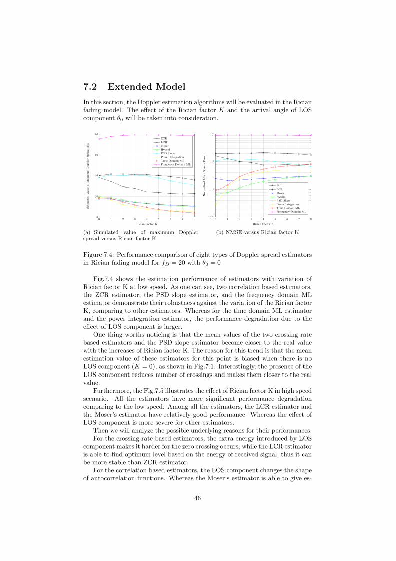
7.2 Extended Model

In this section, the Doppler estimation algorithms will be evaluated in the Ricianfading model. The effect of the Rician factor K and the arrival angle of LOScomponent θ0 will be taken into consideration.

0 1 2 3 4 5 6 7 80

20

40

60

80

Rician Factor K

Est

imate

dV

alu

eof

Maxim

um

Dopple

rSpre

ad

[Hz]

ZCR

LCR

Moser

Hybrid

PSD Slope

Power Integration

Time Domain ML

Frequency Domain ML

(a) Simulated value of maximum Dopplerspread versus Rician factor K

0 1 2 3 4 5 6 7 810−2

10−1

100

101

Rician Factor K

Norm

alize

dM

ean

Square

Err

or

ZCR

LCR

Moser

Hybrid

PSD Slope

Power Integration

Time Domain ML

Frequency Domain ML

(b) NMSE versus Rician factor K

Figure 7.4: Performance comparison of eight types of Doppler spread estimatorsin Rician fading model for fD = 20 with θ0 = 0

Fig.7.4 shows the estimation performance of estimators with variation ofRician factor K at low speed. As one can see, two correlation based estimators,the ZCR estimator, the PSD slope estimator, and the frequency domain MLestimator demonstrate their robustness against the variation of the Rician factorK, comparing to other estimators. Whereas for the time domain ML estimatorand the power integration estimator, the performance degradation due to theeffect of LOS component is larger.

One thing worths noticing is that the mean values of the two crossing ratebased estimators and the PSD slope estimator become closer to the real valuewith the increases of Rician factor K. The reason for this trend is that the meanestimation value of these estimators for this point is biased when there is noLOS component (K = 0), as shown in Fig.7.1. Interestingly, the presence of theLOS component reduces number of crossings and makes them closer to the realvalue.

Furthermore, the Fig.7.5 illustrates the effect of Rician factor K in high speedscenario. All the estimators have more significant performance degradationcomparing to the low speed. Among all the estimators, the LCR estimator andthe Moser’s estimator have relatively good performance. Whereas the effect ofLOS component is more severe for other estimators.

Then we will analyze the possible underlying reasons for their performances.For the crossing rate based estimators, the extra energy introduced by LOS

component makes it harder for the zero crossing occurs, while the LCR estimatoris able to find optimum level based on the energy of received signal, thus it canbe more stable than ZCR estimator.

For the correlation based estimators, the LOS component changes the shapeof autocorrelation functions. Whereas the Moser’s estimator is able to give es-

46

0 1 2 3 4 5 6 7 80

50

100

150

200

250

Rician Factor K

Est

imate

dV

alu

eof

Maxim

um

Dopple

rSpre

ad

[Hz]

ZCR

LCR

Moser

Hybrid

PSD Slope

Power Integration

Time Domain ML

Frequency Domain ML

(a) Simulated value of maximum Dopplerspread versus Rician factor K

0 1 2 3 4 5 6 7 810−3

10−2

10−1

100

Rician Factor K

Norm

alize

dM

ean

Square

Err

or

ZCR

LCR

Moser

Hybrid

PSD Slope

Power Integration

Time Domain ML

Frequency Domain ML

(b) NMSE versus Rician factor K

Figure 7.5: Performance comparison of eight types of Doppler spread estimatorsin Rician fading model for fD = 120 with θ0 = 0

timation based on only two lags, thus it is possible for it to give more stableestimation comparing to the hybrid estimator and the time domain ML estima-tor.

The reason for the sensitivity of PSD based estimators (Including the fre-quency domain ML estimator) is that the LOS components introduced signifi-cant energy on the received signal, so an extra peak will present in the Dopplerspectrum. Thus it differs from the theoretical Jakes’ spectrum significantly. Thepower integration estimator may be affected more seriously since it depends onthe integration of power spectrum.

0 20 40 60 80 100 120 140 160 1800

20

40

60

80

Angle of Arrival of LOS component θ0 (degree)

Est

imate

dV

alu

eof

Maxim

um

Dopple

rSpre

ad

[Hz]

ZCR

LCR

Moser

Hybrid

PSD Slope

Power Integration

Time Domain ML

Frequency Domain ML

(a) Simulated value of maximum Dopplerspread versus θ0

0 20 40 60 80 100 120 140 160 180

10−0.5

100

100.5


Norm

alize

dM

ean

Square

Err

or

ZCR

LCR

Moser

Hybrid

PSD Slope

Power Integration

Time Domain ML

Frequency Domain ML

(b) NMSE versus θ0

Figure 7.6: Performance comparison of eight types of Doppler spread estimatorsin Rician fading model for fD = 20 with K = 2

Moreover, the effect of the angle of arrival of LOS component is shown inthe Fig.7.6 and Fig.7.7. Clearly, the LOS component can has significant impacton the estimation when the angle of arrival is around 90◦, i.e. vertical to the

47

mobile direction.One possible reason is that when θ0 6= 90◦, the LOS component is complex

valued in time domain, and it gives the frequency offset to the received signal. Inthis case, it can be improved by the frequency offset compensation scheme. Onthe other hand, when θ0 = 90◦, the LOS component has real value, so it mayresult in more serious performance degradation on the estimation. However,more investigation on this topic in future is required in order to give morecomprehensive explanation for this phenomenon.

At low speed, the two crossing rate based estimators, the Moser’s estimatorand the power integration estimator are relatively robust to the variation of θ0.The hybrid estimator is affected by the θ0 but is still gives good performance.Whereas at high speed, two crossing rate based estimator and two correlationbased estimators are able to give better performance.

0 20 40 60 80 100 120 140 160 1800

50

100

150

200

250


Est

imate

dV

alu

eof

Maxim

um

Dopple

rSpre

ad

[Hz]

ZCR

LCR

Moser

Hybrid

PSD Slope

Power Integration

Time Domain ML

Frequency Domain ML

(a) Simulated value of maximum Dopplerspread versus θ0

0 20 40 60 80 100 120 140 160 18010−2

10−1

100


Norm

alize

dM

ean

Square

Err

or

ZCR

LCR

Moser

Hybrid

PSD Slope

Power Integration

Time Domain ML

Frequency Domain ML

(b) NMSE versus θ0

Figure 7.7: Performance comparison of eight types of Doppler spread estimatorsin Rician fading model for fD = 120 with K = 2

48

Chapter 8

Conclusions and FutureWorks

The estimation of the maximum Doppler spread is of great importance in avariety of applications in the wireless mobile communications. In this report,four different Doppler spread estimation algorithms are presented and evaluatedfrom both performance and implementation point of view in the WCDMA sce-nario. The algorithms are implemented in BCL for simulation. For deeper andmore comprehensive investigation, both Rayleigh and Rician fading model aresimulated for analysis.

The investigation indicates that the Moser’s estimator is the best choiceamong the four estimators described in this report. The reason is that it givesthe most accurate estimation with relatively low computational cost, and itis relatively robust to the variation of channel properties compared to otherestimators. The correlation based estimators also show their great practicalvalue to implement in applications.

Whereas, the investigation of this thesis is mainly focused on the evaluationand comparison of four types of Doppler spread estimation algorithms. But it isbelieved that the performance of some algorithms can still be improved. Thereare several tasks that can be done for further investigation:

• The adaptive lag selection algorithms for Moser’s estimator can be im-plemented and evaluated. It is believed that this algorithm can furtherimprove the detection accuracy of Moser’s estimator.

• The parametric PSD estimation approach can be applied to improve theestimation accuracy of PSD based estimators.

• The statistic threshold calculation can be implemented to improve thedetection accuracy the PSD slope estimator

These approaches are not tested in the current investigation due to the timeconstraint, but they can potentially increase the accuracy of the estimation.

Moreover, it is also interesting to include and evaluate the potential influ-ence of TPC and AGC on the estimation of Doppler spread. However, thisthesis research can be seen as a reference to the continuous investigation for theDoppler spread estimation in the future.

49

List of symbols

List of Symbols

α Angle between the mobile direction and the average scat-tering direction

B Bandwidth∆B Bandwidth of one interval in PSD slope estimator∆f Detection resolution in ML slope estimatorδ Delta functionη Lag of autocorrelation functionFopt Optimal likelihood function in time domainFsub Suboptimal likelihood function in time domainfD Maximum Dopper frequencyfc Carrier frequencyfd Hypothesis value of maximum Dopper frequency

fD Estimate of maximum Dopper frequencyfshift Doppler shiftγ Signal to Noise Ratio of received signalh Theoretical channel response

h Estimated channel responsehLOS Theoretical LOS component responsehp Theoretical path responseIn Nth order modifiled Bessel function of the first kindJ0 Zeroth order Bessel function of the first kindK Correlation matrix

K Estimation of correlation matrix

K1 Estimation of correlation matrix proposed in [7]

K2 Estimation of correlation matrix proposed in current report-1

kmin Index of interval containing the lowest order peak slope inPSD slope estimator

κ Beam widthLm Maximum lag of correlation functionM Length of slot buffer used in simulationN Number of independent scattered pathsNf Number of received paths (Rake fingers)Nm Size of correlation matrixNs Number of samples in one interval

50

NFFT Number of points for FFTNpilots Number of pilot symbols in each slotωD Maximum Doppler angular frequencyP Power sumation of one interval and its mirror intervalφ0 Phase of the LOS pathφk Phase of the pathrh Autocorrelation function of theoretical channel response

r′

h First derivative of autocorrelation function of theoreticalchannel response

r′′

h Second derivative of autocorrelation function of theoreticalchannel response

ry Autocorrelation function of received signal

r′′

y Second derivative of autocorrelation function of receivedsignal

Sh Power spectral density of theoretical channel responseSy Power spectral density of received signalσB Doppler spread factorσ2h Power of received signalσ2w Power of Gaussian additive noiseTs Sampling periodθ0 Arrival angle of the LOS pathθk Arrival angle of the LOS path kW Doppler spread detection rangew Additive white Gaussian noisey Channel estimate for one DPCCH slotyDPCCH Despreaded, demodulated, received symbols from DPCCH

channel

51

Abbrevations

AWGN Additive White Gaussian Noise

AOA Angle of Arrival Path

BCL Baseband Core Library

CDMA Code Division Multiple Access

DSP Digital Signal Processor

FDMA Frequency Division Multiplex Access

FFT Fast Fourier Transform

GSM Global System for Mobile communication

ITU International Telecommunication Union

LOS Line Of Sight

LCR Level Crossing Rate

ML Maximum Likelihood

NMSE Normalized Mean Square Error

OVSF Orthogonal Variable Spreading Factor

PSD Power Spectral Density

SNR Signal to Noise Ratio

TDMA Time Division Multiplex Access

UE User Equipment

WCDMA Wideband Code Division Multiple Access

52

Bibliography

[1] Zan Li, Jueting Cai, and Jian Shen. Time-variant doppler frequency estima-tion and compensation for mobile ofdm systems. In IEEE Wireless Com-munications and Networking Conference, 2006. WCNC 2006., volume 2,pages 1040–1045, 2006.

[2] Mark D Austin and GL Stuber. Velocity adaptive handoff algorithmsfor microcellular systems. IEEE Transactions on Vehicular Technology,43(3):549–561, 1994.

[3] Goohyun Park, Daesik Hong, and Changeon Kang. Level crossing rateestimation with doppler adaptive noise suppression technique in frequencydomain. In Vehicular Technology Conference, 2003. VTC 2003-Fall. 2003IEEE 58th, volume 2, pages 1192–1195. IEEE, 2003.

[4] Jack M Holtzman and Ashwin Sampath. Adaptive averaging methodologyfor handoffs in cellular systems. Vehicular Technology, IEEE Transactionson, 44(1):59–66, 1995.

[5] Mario Moser. Doppler shift and spread estimation method and apparatus,May 30 2006. US Patent 7,054,394.

[6] Oskar Mauritz. A hybrid method for doppler spread estimation [mobileradio systems]. In Vehicular Technology Conference, 2004. VTC 2004-Spring. 2004 IEEE 59th, volume 2, pages 962–965. IEEE, 2004.

[7] Shantidev Mohanty. Vepsd: a novel velocity estimation algorithm for next-generation wireless systems. Wireless Communications, IEEE Transactionson, 4(6):2655–2660, 2005.

[8] Kareem E Baddour and Norman C Beaulieu. Nonparametric doppler spreadestimation for flat fading channels. In Wireless Communications and Net-working, 2003. WCNC 2003. 2003 IEEE, volume 2, pages 953–958. IEEE,2003.

[9] Mingzheng Cao, Hongya Ge, Hong Zhang, and Ali Abdi. Parametricdoppler spread estimation in mobile fading channels. In Military Com-munications Conference, 2007. MILCOM 2007. IEEE, pages 1–5. IEEE,2007.

[10] Kareem E Baddour and Norman C Beaulieu. Robust doppler spread esti-mation in nonisotropic fading channels. Wireless Communications, IEEETransactions on, 4(6):2677–2682, 2005.

53

[11] Leonid Krasny, Huseyin Arslan, David Koilpillai, and Sandeep Chen-nakeshu. Doppler spread estimation in mobile radio systems. IEEE com-munications letters, 5(5):197–199, 2001.

[12] Aleksandar Dogandzic and Benhong Zhang. Estimating jakes’ dopplerpower spectrum parameters using the whittle approximation. Signal Pro-cessing, IEEE Transactions on, 53(3):987–1005, 2005.

[13] Yuh-Ren Tsai and Kai-Jie Yang. Approximate ml doppler spread estima-tion over flat rayleigh fading channels. Signal Processing Letters, IEEE,16(11):1007–1010, 2009.

[14] Ali Abdi, Hong Zhang, and Cihan Tepedelenlioglu. A unified approach tothe performance analysis of speed estimation techniques in mobile commu-nication. Communications, IEEE Transactions on, 56(1):126–135, 2008.

[15] Ziqi Peng. Performance and complexity comparison of doppler spread es-timation for wcdma systems. MSs thesis project, EES, KTH, 2014.

[16] Elin Palm and Sven Ove Hansson. The case for ethical technology assess-ment (eta). Technological Forecasting and Social Change, 73(5):543–558,2006.

[17] Harri Holma, Antti Toskala, et al. Wcdma for Umts, volume 2006. WileyOnline Library, 2000.

[18] ETSI Specification. 3gpp ts 25.211 version 7.9.0:physical channels andmapping of transport channels onto physical channels (fdd). Physical layerprocedures (FDD), 2009.

[19] Nathan Blaunstein and J Bach Andersen. Multipath phenomena in cellularnetworks. Artech House, 2002.

[20] Tommi Heikkila. Rake receiver. S-72.333 Postgraduate Course in RadioCommunications, 2004.

[21] Gordon L Stuber. Principles of mobile communication. Springer, 2011.

[22] RH Clarke. A statistical theory of mobile-radio reception. Bell systemtechnical journal, 47(6):957–1000, 1968.

[23] Ali Abdi, Janet A Barger, and Mostafa Kaveh. A parametric model for thedistribution of the angle of arrival and the associated correlation functionand power spectrum at the mobile station. Vehicular Technology, IEEETransactions on, 51(3):425–434, 2002.

[24] Cihan Tepedelenlioglu, Ali Abdi, Georgios B Giannakis, and MostafaKaveh. Estimation of doppler spread and signal strength in mobile commu-nications with applications to handoff and adaptive transmission. WirelessCommunications and Mobile Computing, 1(2):221–242, 2001.

[25] Mehrez Souden, Sofiene Affes, Jacob Benesty, and Rim Bahroun. Robustdoppler spread estimation in the presence of a residual carrier frequencyoffset. Signal Processing, IEEE Transactions on, 57(10):4148–4153, 2009.

[26] Raj Jain. Channel models a tutorial1. 2007.

54

Comparison and Evaluation of Doppler Spread …749322/FULLTEXT01.pdf · 2.1 Example of the...

Documents

Transcript of Comparison and Evaluation of Doppler Spread …749322/FULLTEXT01.pdf · 2.1 Example of the...