Comparing empirical models of the euro economy - …€¦ · · 2006-11-14Comparing empirical...

Economic Modelling 21(2004) 735–758

0264-9993/04/$ - see front matter� 2003 Elsevier B.V. All rights reserved.doi:10.1016/j.econmod.2003.10.003

Comparing empirical models of the euroeconomy

Kenneth F. Wallis*Department of Economics, University of Warwick, Coventry CV4 7AL, UK

Abstract

This article presents a comparative analysis of four macroeconometric models whoseproprietors participated in a model comparison conference focused on the new euro areaeconomy. One model, the Area-Wide Model recently developed at the European CentralBank, treats the whole area as a single economy. The other three, MULTIMOD, NIGEM andQUEST, are established multicountry models that provide disaggregated analysis of questionsof economic policy in Europe. Their structural characteristics and the results of two policysimulations are compared and contrasted. The principal source of simulation differences isthe different degree of forward-looking behaviour incorporated in the models.� 2003 Elsevier B.V. All rights reserved.

JEL classifications: C5; E1

Keywords: Macroeconometric models; Multicountry models; Model comparisons; Simulation; Euro-area economy

1. Introduction

On 1 January 1999 the third and final stage of European Monetary Union began,with the irrevocable fixing of exchange rates between the currencies of the elevenEU members initially participating in Monetary Union, and with the conduct of asingle monetary policy under the responsibility of the European Central Bank. Theprimary objective of monetary policy is to maintain price stability in the euro areaas a whole, hence new challenges were faced by the econometric models employedin forecasting and policy analysis.

*Tel.: q44-24-7652-3055; fax:q44-24-7652-3032.E-mail address: [email protected].

736 K.F. Wallis / Economic Modelling 21 (2004) 735–758

One response was to provide an area-wide focus directly, by developing amacroeconometric model that treats the whole area as a single economy. Thisprecludes the consideration of the possibly different impacts of a common policyon different countries, and a system of linked national-economy models is underdevelopment within the Eurosystem to provide this. In the meantime existingmulticountry models are an alternative source of such analysis, and the objective ofthe present model comparison exercise is to evaluate the advantages and disadvan-tages of the different approaches. Along with the Area-Wide Model(AWM) of theEuropean Central Bank(Fagan et al., 2001), the model comparison exercise featuresthree well-established multicountry models, namely

● MULTIMOD Mark III, developed in the Research Department of the InternationalMonetary Fund in Washington, DC(Laxton et al., 1998), with further Europeanextensions for this exercise,

● NIGEM, developed at the National Institute of Economic and Social Research,London(Barrell et al., 2001), and

● the QUEST model of the European Commission(Roeger and in’t Veld, 1997).

The present exercise is in the style of a model comparison conference based onmaterial supplied by the model proprietors, describing model exercises that theyhave carried out, as distinct from a third-party comparative research project, basedon implementation of the models by independent researchers. The differencesbetween the two styles of model comparison are discussed by Mitchell et al.(1998)in introducing the results of their independent third-party research on three multi-country models, among which are earlier versions of MULTIMOD and NIGEM.Structural change and aggregation questions are at the heart of the modelling

challenges presented by the final stage of European Monetary Union, although bothhave a long history, in the context of EMU and more generally. Structural changein models reflects changes in the problems they address and changes in theeconomies they represent. For potential EMU members the approach to monetaryunion increased the attention paid to the various convergence criteria, leading tosubstantial changes in fiscal policy. The final move to a single currency and a singlemonetary policy was the culmination of a series of policy changes over the previoustwo decades, as quantitative controls were abandoned, financial liberalisationproceeded apace, and monetary policy focussed more directly on the control ofinflation. With exchange rate risk among member countries removed and transactionscosts reduced the consequences continue, as the whole spectrum of interest ratesconverges and financial markets deepen. A structural rather than reduced formmodelling approach is clearly needed to reflect these changes and their consequences,as is argued with detailed examples from the present context by Maclennan et al.(2000), for example.Aggregation issues are central to the comparison of area-wide and individual

country modelling, and have a theoretical literature that starts in the middle of thelast century(Klein, 1946; Nataf, 1948; Gorman, 1953; Theil, 1954). The technicalliterature considers such questions as the conditions for ‘perfect’ aggregation andtests thereof, and statistical discrimination between aggregate and disaggregate

737K.F. Wallis / Economic Modelling 21 (2004) 735–758

models. A typical result is that, given linear regression models for an aggregatevariable and each of its several components, the goodness of fit of the aggregatevariable obtained by summing the fitted values of the component models is noworse than that of the aggregate model, and is potentially much better the morediverse are the component models. However, such results are usually obtained underthe assumption that the various models are correctly specified, whereas specificationuncertainty is endemic, and little is known about its impact. The more componentsthere are to be modelled, the greater the opportunities for specification error. Withrespect to model specification in the non-linear case, which is more relevant forpractical macroeconometric models, an important observation by Stoker(1986) isthat models estimated with aggregate data contain distributional biases that are notmeasurable using aggregate data alone; time series of distributional data are requiredto correct these effects. Distributional movements are typically small, hence theireffects may tend to persist in aggregate data over many periods, increasing theapparent explanatory power of lagged variables if they are ignored.There is also much literature on country differences across Europe and their

implications; see again Maclennan et al.(2000) and references therein. Only a smallpart of this is quantitative or model-based, and here a general conclusion seems tobe that, for problems for which an aggregate measure of outcomes is appropriate,the differences between using an aggregate analysis and adding together the resultsof disaggregated analyses are not dramatic. If distributional effects appear in theloss function, however, then only a disaggregated analysis can provide an answer.They do not feature in decision-making by the European Central Bank, whichalways adopts an area-wide perspective, but they may become a concern of nationalpolicy agencies, should differences in economic developments across countriesthreaten to become too large. Distributional matters may also affect the area-wideaggregates that the ECB targets, as noted above, hence they may become a matterof concern for the ECB even though they do not feature directly in its objectives.The present model comparison exercise provides a first model-based evaluation ofthe nature and scale of such effects in a euro area setting.The remainder of this article is organised as follows. Section 2 contains a

comparative account of the structural characteristics of the four models, as deter-mined by their underlying theoretical foundations and their empirical implementa-tion, and two key areas are emphasised. The first is the supply side andinflation-unemployment nexus of the models, where a core supply-side frameworkis used to organise the discussion. The second area of the models that is emphasisedis their treatment of consumption and investment decisions. Section 3 is concernedwith two simulation experiments that demonstrate the responses of the models tofiscal and monetary policy shocks. Issues of experimental design are first discussed,and then the simulation results are compared across models and across countries. Itis seen that some of the differences that emerge can be related to structural featuresof the models elucidated in the preceding section. Section 4 contains concludingcomments.


2. Four models of the euro economy

2.1. General characteristics

The Area-Wide Model(AWM) of the European Central Bank treats the euro areaas a single economy, as noted above. It corresponds to a conventional national-economy macro model, with the rest of the world treated as exogenous. Althoughthis includes the three EU members that have not adopted the single currency, andGreece, which did not join the third stage of EMU until 1 January 2001, in thecurrent model the rest of the world is proxied by a four-country aggregate, comprisingthe United States, Japan, the United Kingdom and Switzerland. The euro areadataset used in the model is based on reconstructed euro area national accounts dataconsistent with individual member-country data, carefully aggregated. The maindiscrepancy between the constructed euro area accounts and conventional nationalaccounts arises in the trade data, where the constructed data include both tradewithin the areay between member countries – and trade with the rest of the world.In contrast to national-economy models, global economic models focus on

macroeconomic interactions among nations. Although the three global models underconsideration describe the same world they differ in respect of which countries aremodelled individually and how the remaining countries are grouped together. Theoriginal Mark III version of MULTIMOD (Laxton et al., 1998) contains separatemodels for each of the Group of Seven(G7) countries – the US, Canada, Japan,France, Germany, Italy, UK – and for an aggregate grouping of 14 smaller industrialcountries. The remaining economies of the world are then aggregated into twoseparate blocks of developing and transition economies. Each of the industrial-country models has the structure of a complete national-economy model, whereasthe two remaining blocks are modelled in much less detail, focussing on foreigntrade and the evolution of net foreign assets in a more reduced form than structuralmanner. The first modified version of the model used in the present exercise has aseparate subgroup of ‘other euro area’ countries, whose results can be combinedwith those of France, Germany and Italy to obtain euro area macroeconomicoutcomes. The second modified version(Mark IIIB) has a single euro area blockand is estimated on more recent data.NIGEM and QUEST are more disaggregated, each having complete country

models for each EU member(taking the Belgium-Luxembourg Economic Union asa single entity) and a finer division of the rest of the world. After separate countrymodels for the remaining three G7 members, NIGEM has six intermediate-sizemodels consisting of a very basic description of the domestic economy(output andprices) together with trade volume and price equations and the balance of payments;these relate to Australasia, Mexico, Norway, S. Korea, Switzerland and the Visegradeconomies(Czech Republic, Hungary, Poland). Finally, there are seven simplertrade-and-payments models for China, OPEC, Developing Europe, Africa, LatinAmerica, other LDCs, and the rest of E. Asia. QUEST separately models the USand Japan, then describes the rest of the world by 11 trade-and-payments models.Four of these relate to the larger remaining OECD countries(Australia, Canada,


Norway, Switzerland) and seven to various groups of countries, very much as above(Central and Eastern Europe, the rest of the OECD, OPEC, the former SovietUnion, ‘dynamic’ Asian economies, the rest of Asia, and the rest of Africa andLatin America).The theoretical foundation of the complete national-economy submodels is

common to all countries in each case, and also has common elements across thefour models. All follow the currently prevailing paradigm in which a broadlyneoclassical view of macroeconomic equilibrium coexists with a new Keynesianview of short-to-medium-term adjustment. The simple Mundell-Fleming modelremains the basic underlying model of interdependence, but it is considerablyextended, by adding dynamics, modelling the processes generating aggregate supply,accounting for the behaviour of asset and debt stocks as well as financial flows,and endogenizing fiscal and monetary policy. All the models incorporate forward-looking behaviour in financial markets and, in some cases discussed below, indecision-making by firms and households; they all treat future expectations as‘rational’ or ‘model-consistent’ expectations. Some important differences acrossmodels andyor countries that nevertheless appear in two key areas are described inthe following sub-sections.Two potential sources of such differences are different relative weights on theory

and data in the specification of the models, and different approaches to quantification.MULTIMOD and QUEST have more thoroughly elaborated theoretical foundations,particularly with respect to the steady state of the models, than AWM and NIGEM,whose steady state properties are based more on the use of cointegration techniquesin estimation, with long-run coefficients sometimes imposed following pre-testing.MULTIMOD is an annual model, and sometimes compensates for the resulting lackof degrees of freedom in estimation by using pooled estimation methods, whereuponnot only the equation specifications are common to all countries but also theircoefficient estimates. The three ‘European’ models are quarterly and make less useof pooled estimation, NIGEM allowing different dynamic specifications acrosscountries to emerge in estimation. However, QUEST’s dynamic responses also havea more theoretical basis, and its emphasis on theoretical foundations sometimesresults in the calibration of key parameters rather than their estimation fromaggregate time series data.The terms equilibrium, long run, and steady state are used interchangeably in this

discussion, and all refer to the steady-state properties of a system of dynamicequations, designed in the present context for short-to-medium-term forecasting andpolicy analysis. Thus the range of issues considered under the heading of ‘long-runimplications«’ is only a subset of what economists more generally might wish toconsider as long-run issues. Here the long-run equilibrium is a steady-state growthpath for the aggregate real and nominal variables of the model, with constantinflation. The steady-state real growth rate is equal to the natural growth rate of thestandard neoclassical growth model, equal to the rate of(labour-augmenting)technical progress plus the growth rate of the population, both treated as exogenous.Nominal equilibrium is ‘anchored’ by specifying a target, again exogenously, for anominal variable such as inflation, with the target value typically achieved in steady


state via an appropriately specified feedback rule for nominal interest rates, asillustrated in our simulations.The study of steady-state properties proceeds in various ways. In MULTIMOD

each of the dynamic equations has an explicit steady-state analogue equation, andthe complete system of steady-state analogue equations is maintained separatelyfrom the system of dynamic equations, to provide an interpretative device forunderstanding long-run comparative statics and to facilitate model handling byproviding terminal conditions for model-consistent expectations solutions. In theremaining models there is no formal description of the steady state, although itstheoretical properties are well understood, and it is studied by simulation methods.In a deterministic solution of the complete system of non-linear equations eachindividual equation holds exactly(to a numerical approximation) and hence has animplicit steady-state counterpart, at least in the neighbourhood of the solution. Forsome equations it may be possible to obtain an explicit steady-state representation,whereupon partial or sub-system analysis can proceed by analytical methods, as insome examples below.

2.2. The supply side and the inflation-unemployment nexus

The prevailing paradigm noted above implies that at least in respect of the long-run equilibrium, the level of real activity is independent of the price level and thesteady-state inflation rate, whereas in the short run there is considerable real andnominal inertia. Adjustment costs and contractual arrangements imply that marketsdo not clear instantaneously; instead there is a relatively slow process of dynamicadjustment to equilibrium. This is by no means a full-employment equilibrium,however, and important questions are whether a model possesses a non-accelerating-inflation rate of unemployment(NAIRU) and, if so, what are its determinants. Ifthese determinants do not include the steady-state inflation rate then the NAIRUcoincides with the ‘natural’ rate of unemployment.The underlying theoretical framework of the three European models, like that of

many national-economy models in Europe, is one of imperfectly competitive goodsand labour markets, with prices set by firms as a mark-up on costs, given demand.Wages are determined in a bargaining process and if firms have the ‘right tomanage’ they set employment, given the wage, although wage behaviour is relativelyinsensitive to the particular specification of the bargaining model. The precedingquestions about the NAIRU or, equivalently, whether the aggregate supply scheduleis vertical and what causes it to shift, can then be addressed by analysing a coresupply-side model consisting of the steady-state versions of the wage and priceequations together with, in an open-economy context, the response of the exchangerate(Joyce and Wren-Lewis, 1991; Turner, 1991). We first present a simple algebraicrepresentation of this ‘core’ system(Wallis, 2000), and then use it as a frameworkfor comparison of the four models. We note that MULTIMOD, in contrast to theEuropean models, but like several North American models, assumes that firms areperfectly competitive and have no mark-up opportunities.


Long run: Given wage and price equations expressed in error-correction form, thefirst step is to solve the long-run or error-correction parts of the equations for theNAIRU, which requires their static homogeneity. The long run of a typical wageequation may be written

wwspqpryauqz (1)

wherew, p and pr are (log) nominal earnings, producer prices and average labourproductivity, respectively,u is the unemployment rate(entered linearly for simplicity)and z is a set of wage pressure variables. A typical assumption about pricingw

behaviour is that producer prices are determined as a mark-up on import and unitlabour costs, with the mark-up increasing with capacity utilization(cu), hence

psbp q(1yb)(wypr)qgcu, (2)m

wherep is the import price. The capacity utilization term would not appear if anm

equilibrium state were defined as one in which output coincides with ‘normal’output; it may also be related to unemployment. Static homogeneity is implicit inthe unit coefficients in Eq.(1) and the unit sum of the first two coefficients in Eq.(2); these restrictions are usually found to be data-admissible.The real exchange rate is defined as

qspyp . (3)m

Substituting forp from Eq. (3) and then solving Eqs.(1) and (2) gives them

equilibrium rate of unemployment as

w z1 b g* wu s z y qq cu .x |a 1yb 1yby ~

Dynamic equations: The error-correction formulation expresses the dynamic equa-tions in terms of the first differences(Ds) of the (log) levels of wages and prices,that is, the wage and price inflation rates, together with lagged values of these andother variables expressed in similar form, except for the levels variables that appearin the error-correction term itself. Thus, deleting dynamic terms in other variablesand the time subscript for convenience, we have

f (L)Dwsu (L)Dpqc (L)Dpryd ec(w) (4)1 1 1 1

f (L)Dpsu (L)Dcostyd ec(p) (5)2 2 2

wheref(L) etc. are polynomials in the lag operatorL, which may include forwardterms,ec(w) andec(p) are the error-correction terms given as the(lagged) residuals


from Eqs.(1) and (2), respectively, and the cost terms have been combined into asingle variable.We consider a steady state with a constant rate of price inflationp in all countries

(and hence constant nominal exchange rates), and constant real wage growth equalto the rate of growth of productivity, that is

DpsDp sDcostspm

DwspqDprspqg.

Other first-difference terms that appear are set to zero, for example, the wage-pressure variables are assumed constant. In such a steady state, Eqs.(4) and (5)then give the NAIRU as

S Wc 1 yf 1 u 1 yf 1 u 1 yf 1T TŽ . Ž . Ž . Ž . Ž . Ž .1 1 1 1 2 21 1† * U Xu su q gq q p.T Ta d a V d d Y1 1 2

This is the natural rate of unemployment, independent ofp, if the expression incurly brackets is zero. A sufficient condition is that each of the two terms in thecurly brackets is zero, that is, that the wage and price equations are dynamicallyhomogeneous or inflation neutral. In empirical work on the European economiesthis is more commonly found to be the case for wage equations than for priceequations.It is found in some countries that the wage equation is not dynamically

homogeneous with respect to productivity, withc (1)-f (1), so that in a dynamic1 1

steady state with real wage growth occurring at the rate of growth of productivity,this steady-state productivity growth rate affects thelevel of real wages and theNAIRU: lower productivity growth gives a higher natural rate of unemployment.This is consistent with the evidence of Manning(1992) that the slowdown inproductivity growth was an important explanation of the increase in unemploymentin many OECD countries. It suggests that, of the two competing effects of growthon unemployment identified by Aghion and Howitt(1994), the ‘capitalisation’effect, whereby an increase in growth raises the capitalised returns from creatingjobs and consequently reduces the equilibrium unemployment rate, empiricallydominates the ‘creative destruction’ effect.

Taxation: If the relevant taxes are identified in the model, then different real wageconcepts are relevant to the objectives of the two parties to the wage bargain. Foremployers, what matters are their real wage costs(wqt yp), namely nominale

wages plus employment taxes deflated by producer prices, whereas employees focuson the real consumption wage(wyt yp ), namely nominal wages less direct taxesd c

deflated by consumer prices(p , in logs, with average tax ratest and t expressedc e d

as proportions). The difference between the two is the tax wedge

(wqt yp)y(wyt yp )st qt qp yp.e d c d e c


Let l be the weight of domestic goods in(pre-tax) consumer prices, so that the(post-tax) consumer price variable is

p slpq(1yl)p qtc m i

wheret is the average indirect tax rate. Then the wedge is given asi

wedgest qtqt qt ,d i e m

where t s(1yl)(p yp) is the ‘tax’ imposed by high import prices; thesem m

definitions imply thatp spqt qt .c i m

This formulation has two implications for the wage equation. The first is that allfour tax variables, treated as wage-pressure variables, have the same effect; it iscustomary to combine them into a single tax wedge variable, which also avoids thestatistical difficulties of accurately estimating the separate effects of variables whichtypically show relatively little variation over the sample. The second implication isthat, in order to assess the incidence of taxation, the wage equation should bespecified with one or other of the two after-tax real wage variables as dependentvariable. Choosing employers’ real wage costs, for example, Eq.(1) becomes

w(wqt yp)spryauqr(t qtqt qt )qotherz variables,e d i e m

where r is a measure of the incidence of taxation. A null hypothesis of interestmight then be thatrs0, conforming to the view that, in the long run, rises in thewedge are borne entirely by labour. Short-run wedge effects may nevertheless beimportant and rather persistent, withD(wedge) appearing in the error-correctionform of the wage equation.A final observation on this analysis is that the answers to some important ‘long-

run’ questions are seen to depend on the specification of the short-run or dynamicadjustment parts of the equations, in contrast to the very sharp separation found inthe cointegration literature between the long-run and short-run implications ofstatistical models. Constant terms have not featured in the analysis, whereas theyare often present in estimated equations. Johansen(1991) draws the importantdistinction between the two roles of a constant term in the vector error-correctionmodel: one contributes to the intercept in the cointegrating relation while the otherdetermines a linear trend(exponential trend in the case of a log-linear model). Heprovides a procedure for testing that the trend is absent, although this is notapplicable in the single-equation case, where the allocation between the two rolesis at the disposition of the modeller, as in some examples below.

AWM: The key wage and price equations of AWM are similar in appearance tothe above core model, but differ from it in important ways. The wage equation is

e 2 2D wyp ypr s0.27D wyp ypr q0.2p yDp qu L D p qc L D prŽ . Ž . Ž . Ž . Ž .y1c c c,y1 1 c

w zx |y0.015uyutr y0.10wyprypyln 1ybŽ . Ž .y1 y ~y1


wherep is the consumption deflator,p is the GDP deflator at factor cost,u is thec

unemployment rate, its trend, andwypr denotes trend unit labour costs(all inutr –––––

logs); p is inflation expectations. Despite using different price deflators in thee

long-run and short-run parts of the equation there is no consideration of wedgeeffects, nor any other wage pressure variable. In the long run real unit labour costsare equal to labour’s share, in turn equal to the labour elasticity in the productionfunction, 1yb. Dynamic homogeneity holds, but since the unemployment term isthe deviation of unemployment from the exogenous NAIRU the statement that ‘thelong-run Phillips curve is vertical in the model’ has less empirical content here thanin our core model.The price equation contains the same error-correction term(whose sign is changed

above to maintain the usual convention of a negative coefficient), as follows:

eDps0.0039q0.23Dp q0.2p yDp q0.03ygap q0.031DpŽ .y1y1 y1 m,y1

w zx |qu L D wypr y0.045 py wypr qln 1ybŽ . Ž . Ž . Ž .2 y ~y1

Dynamic homogeneity is strongly rejected by the data, which is interpreted asimplying that ‘in principle the mark-up in the long run depends on steady stateinflation’ (Fagan et al., 2001, p. 17). Solving the steady-state version of theestimated equation for a common steady-state rate of inflation of domestic andforeign prices and unit labour costs gives a rate of 0.0039y(1y0.746)s0.015 perquarter or 6% per annum, which is close to the average inflation rate of the GDP(at factor cost) deflator over the sample period. In simulation exercises the constantterm is adjusted to ensure that ‘the long-run real equilibrium of the model coincideswith the theoretical steady state’ at an inflation rate, in the present case, of 2% perannum.

MULTIMOD: Like its predecessors, Mark III has no labour markety noemployment and wage equations. Wage setting is subsumed with price setting intoa ‘Phillips curve’ described as a reduced-form relationship between(price) inflationand unemployment. The latter variable is of course endogenous in the model; theinflation equation is in reduced form in the sense that it can be derived from a two-equation system as above by substituting the wage equation into the price equation(Laxton et al., 1998, Box 6; Sgherri, 2000, Appendix). Unemployment enters non-linearly, to reflect increases in the degree of real wage rigidity as the unemploymentrate rises. The equation is

*B Euyue C Fpslp q 1yl p ygŽ .q1 y1D Guyf

wherep , u andf are constructed proxy series,u representing a NAIRU concept.e * *


Coefficient estimates for the three main euro-area countries are

France ls0.75 gs0.011Germany ls0.74 gs0.008Italy ls0.91 gs0.023

The non-linearity of the equation implies that country responses to an aggregatedemand shock may depend not only on these coefficient differences but also ondifferences in their relative initial positions. A supply-side shock can be implementedby directly perturbing the NAIRU.The inflation-unemployment nexus is closed by an unemployment equation that

translates output gaps , where is an estimate of potential output, into¯ ¯yyy yunemployment gaps , where is an estimate of the natural rate. The equation¯ ¯uyu uis

¯ ¯ ¯uyu sg yyy qg uyuŽ . Ž . Ž .y11 2

France g sy0.30 g s0.441 2

Germany g sy0.33 g s0.181 2

Italy g sy0.09 g s0.791 2

It is sometimes described as a derived demand for labour function, but it has noprice effects and assumes constant labour supply.

NIGEM: The general structure of the wage and price equations of NIGEM andtheir delivery of the NAIRU is very close to our core model. The wage equationsexhibit static and dynamic homogeneity. They contain a mixture of forward-lookingand backward-looking terms in price inflation, and in terms of the degree of forward-lookingness the three main euro-area economies are ranked in the same order as inMULTIMOD’s Phillips curve, namely Italy, France, Germany.(In both models thecorresponding UK equation is entirely forward-looking.)Price setting refers to a CES cost function, hence producer prices are driven by

the user cost of capital as well as import prices and unit labour costs. Then theNAIRU in turn depends on the equilibrium real interest rate. The price equations inall countries have static homogeneity, but dynamic homogeneity is less widespread.In particular, the UK price equation is dynamically homogeneous whereas those ofFrance, Germany and Italy are not, as in the corresponding euro area specificationof AWM. Again the interpretation is that the mark-up depends on the inflation rate.

QUEST: The labour market specification in QUEST is based on theoreticalsearch models, nevertheless wage bargaining results in a wage equation of thegeneral form discussed above. A specific wage pressure variable is the reservationwage, equal to the pre-tax value of unemployment benefits, and so both the incometax rate and the benefit rate affect the NAIRU. A supply-side shock that affects thelong-term unemployment rate can be implemented by perturbing the reservationwage, whereas AWM and MULTIMOD tell no story about what it is that alters theNAIRU and what other effects it might have in the model. Dynamics in QUESTare explicitly based on staggered contracts, hence expected future prices for theduration of the contract appear in the equation.


The price equation in the present version of the model is a version of the ‘hybrid’equation with forward-looking and backward-looking pricing behaviour estimatedon the AWM dataset by Gali et al.(2001). The inflation dynamics are common toall countries, and the forward coefficient of 0.7 is close to the correspondingestimates for France and Germany in MULTIMOD, although in that model othercountries take different values and the change of data frequency should be noted.Sensitivity to the output gap is lowest in Germany, again as in MULTIMOD. Thework of Gali et al.(2001) is an extension to the euro area of the ‘New KeynesianPhillips Curve’ estimated on US data by Gali and Gertler(1999). The original USequation is subjected to rigorous testing, which it does not survive, by Rudd andWhelan(2001, 2002). Its European counterpart suffers a similar fate at the handsof Bardsen et al.(2002), who also report similar findings for Norway and theUnited Kingdom. Likewise, Balakrishnan and Lopez-Salido(2002) find that theNew Phillips Curve performs badly in the United Kingdom.

2.3. Consumption and investment decisions

Consumption: The general framework for the analysis of consumers’ expendituredecisions is the Blanchard-Yaari life-cycle model of intertemporal optimization byfinitely-lived households, moderated by a proportion of households who are unableto implement full intertemporal optimization because of financial constraints and soconsume their current disposable income. The models differ in their relative weightson theory and data, as noted above. MULTIMOD and QUEST pay more detailedattention to the underlying framework and its ‘deep’ parameters, whereas AWM andNIGEM simply report an aggregate ‘solved out’ consumption function, usingMuellbauer and Lattimore’s(1995) term; this is in error-correction form.

AWM: The short-run part of the error-correction equation in the present versionof the AWM model includes current and lagged income growth, together with adirect real interest rate term. In the long run consumers’ expenditure is related todisposable income and wealth, with elasticities 0.65 and 0.35, respectively. Wealthis defined as cumulated savings, assuming that households own all the assets in theeconomy, namely public debt, net foreign assets and the private capital stock, hencethere are no asset price effects.

MULTIMOD: The theoretical framework in MULTIMOD incorporates a concavelife-cycle profile of labour income, rising with age and experience when individualsare young, and eventually declining with retirement. This is estimated from data onlabour income and employment by age cohort for the US, and these estimates arethen used in all other industrial countries. Laxton et al.(1998, Table 10) report aG7 pooled estimate of 0.41 for the intertemporal elasticity of substitution, andcountry-specific estimates of the sensitivity of consumption to disposable income.These imply unusually large estimates of the share of income-constrained consump-tion, and the new estimates in Mark IIIB reduce this to 44% for the euro area.

NIGEM: The consumption function in NIGEM has the same long-run form asAWM, but adjustment behaviour is forward looking. Panel estimation of commonparameters for Europe(but not the UK) yields a greater long-run elasticity with


respect to income of 0.83 in Europe and 0.86 in the UK. The wealth measure isfinancial wealth.

QUEST: The consumption model in QUEST, like that in MULTIMOD, isformulated in terms of deeper parameters. The share of liquidity-constrainedconsumption is set at 0.3 in all countries, since individual country estimates basedon Euler equations do not differ significantly from this. The intertemporal elasticityof substitution for unconstrained consumers is calibrated at 0.5, having in mindestimates in the literature from both aggregate time series data and household surveydata.

Investment: In AWM and NIGEM the behaviour of investment is a process ofdynamic adjustment to a steady state described by factor demand equations consistentwith the underlying production function. A Cobb–Douglas production function isassumed in AWM, and the investmentyoutput ratio responds to deviations of theratio of investment to potential output from its implied steady-state value. This is afunction of the user cost of capital, the variable component of which is representedin the model equation by the short-term real interest rate. The underlying technologyin NIGEM is CES, as noted above, and estimates of the elasticity of substitutionfor each country are obtained from the labour demand functions. These determinethe steady-state capitalyoutput ratio, with the user cost of capital depending on thelong real rate of interest. The response to a temporary shock to nominal interestrates might then be expected to be more muted than in AWM. There is a littlevariation in the dynamics of adjustment across countries in NIGEM.In contrast MULTIMOD and QUEST adopt the model of intertemporal optimi-

zation by firms based on Tobin’sq theory. While theoretically attractive, in particularspecifying a role for profit taxes, this is difficult to implement econometrically. InMULTIMOD a common equation is based on a panel of the industrial countries,whereas in QUEST, as in NIGEM, there is some variation in the dynamics ofadjustment across countries.

3. Two simulation experiments

3.1. Experimental design

Our comparative analysis is based on the results of the fiscal policy and monetarypolicy simulations, focusing on the outcomes for GDP and inflation. The simulationswere carried out by the model proprietors under conditions that were standardisedas far as possible, and full results are presented in their separate articles(Barrell etal., 2004; Dieppe and Henry, 2004; Hunt and Laxton, 2004; Roeger and in’t Veld,2004).The fiscal shock is a reduction in government spending of 1% of GDP, and the

monetary shock is an increase of 1% point in the nominal short-term interest rate.Both are unanticipated temporary shocks, maintained for 1 year(four quarters).During this period the models’ normal policy reaction functions are switched off,and then reintroduced once the temporary perturbation is over. In the fiscal shockthis implies that the relevant policy instruments, namely a fiscal tax rate and the


nominal short-term interest rate, are held at their base-run values in the first year;in the monetary shock the fiscal instrument is again held at base, whereas it is themonetary policy instrument that is perturbed.Standardisation of policy regimes remains a contentious issue. Mitchell et al.

(2000) argue, in the light of their own analysis and the experience of the secondBrookings model comparison project(Bryant et al., 1993), that it is not enough toask modellers to run simulations ‘with their normal tax-rate reaction functions inplace’. They show that the ‘normal’ fiscal policy rules on some leading modelsdiffer substantially in their impact on simulation results. In the present exercise thevariation among rules is much less, however, since all four models operate tax-difference rules that target either the debtyGDP ratio (MULTIMOD, QUEST) orthe deficityGDP ratio(AWM, NIGEM), and Mitchell et al.(2000) show that it isimmaterial whether the exogenous targets are expressed in terms of the debt or thedeficit, provided that the choices are mutually consistent. The parameterisation ofthe rules determines the nature and speed of the dynamic adjustment of their targetvariables, and here too different rules can be adjusted to give equivalent outcomeson a given model. These are a function not only of the rule but also of the model’sintrinsic dynamics, however, and standardisation of the performance of differentrule-model combinations may be necessary to obtain a sharp comparative focus onother areas of the models. But this would require experimentation that is beyondthe scope of the present exercise, and the normal tax-rate reaction functions wereaccordingly left in place. With respect to monetary policy, there has been muchconvergence in recent years towards interest-rate rules that target inflation. Althoughdifferences in their normal rules remain across the models there was interest amongthe modellers in standardising on a ‘Taylor’ rule that also targets the output gap,with coefficients 1.0 and 0.25 on the inflation and output terms, respectively. In theevent additional results under a variety of monetary policy rules are also reportedfor all models except MULTIMOD, which only considers this standard Taylor rule.The organisers of the first Brookings multicountry model comparisons(Bryant et

al., 1988) also attempted to standardise the simulation baseline path, in order topromote comparability of simulation results by eliminating potential base depend-ence. Non-linearity in models is usually cited as a possible source of basedependence, a practical example being provided by the study of the impact ofstarting point conditions on fiscal multipliers in the accompanying article by Huntand Laxton. One response is to apply relatively small shocks in simulations andrely on local linearity. Even in the absence of complicated non-linear functions,however, stock-flow effects can be seriously influenced by differences in baselinestocks. The example cited by Bryant et al.(1988, p. 30) is the stock of governmentdebt, where ‘differences in baseline debt stocks can alter significantly the simulatedeffects of a change in interest rates’. This example is relevant to the present exercisewhere, in particular, the different models’ base solutions incorporate differentassumptions about the evolution of public debt in Italy towards the MaastrichtTreaty target of 60% of GDP. In the event the Brookings project failed to achieve acommon base solution across models, and it has not been attempted here. Thesolution period typically begins in the recent past, and differences become more


pronounced further out into the future. The responses to temporary shocks appliedat the beginning of the period, on which this article focuses, are less likely to bevulnerable to differences in the baseline than the results of permanent shocks.To analyse possible differences across countries and the consequences of aggre-

gation the fiscal shock is applied, where possible, to the major EU economies oneat a time and to the euro area as a whole, and in both cases results are presented,where possible, for individual countries and the aggregate. The area-wide shock andits area-wide consequences are all that AWM and MULTIMOD Mark IIIB canconsider, while MULTIMOD Mark III describes the consequences of an area-wideshock for France, Germany, Italy and ‘other’ euro area, which are cumulated to givethe area-wide responses. Mark III also considers country-specific shocks, andNIGEM and QUEST are operated mostly in this mode. Reflecting the introductionof a single monetary policy, the monetary shock is applied area-wide, and contrastedwith a worldwide perturbation to interest rates. Again, where possible, results arepresented for individual countries and the euro area as a whole.Tables 1–4 provide a summary comparison of the GDP and inflation responses

in fiscal and monetary policy simulations under the ‘standard’ Taylor rule discussedabove. For each model the inflation measure reported is the variable that appears inthe rule, either the GDP deflator(PGDP) or the consumers’ expenditure deflator(CED). Other material discussed below is extracted from the modelling groups’tabulations as required, without detailed cross-referencing.

3.2. Fiscal policy simulation results

The responses of GDP to the fiscal contraction show wide variation, with impactmultipliers well in excess of one on AWM and MULTIMOD, and somewhat belowone on NIGEM and QUEST. These apparent pairwise similarities mask importantdifferences, however.Taking AWM and MULTIMOD first, we focus on the euro area concurrent

responses to the area-wide shock. Expressing the components of the familiar nationalincome identityYsCqIqGq(XyM) as percentages of baseline GDP gives themultiplier decompositions

AWM:y1.35sy0.72y0.54y1.0q0.91

MULTIMOD:y1.48sy0.60y0.01y1.0q0.13

With the nominal interest rate held at base during the first year, and inflation beingreduced, the real short rate rises, and this has a strong direct effect on consumptionand investment, both fixed investment and stockbuilding, in AWM. Each of thethree endogenous components also responds directly to the fall in demand, the tradebalance especially so, due to the strong response of imports to lower GDP, althoughthe inclusion of intra-area trade raises questions about the quantification of thiseffect. With respect to investment, MULTIMOD’s intertemporal optimisers recognisethe temporary nature of the perturbation, and scarcely change their actions. Forward-


Table 1Fiscal shock, real GDP responses(percent deviation from base)

France Germany Italy Euro area

Area-wide shock

AWMYear 1 y1.352 y0.523 0.095 0.2210 0.03

MULTIMOD IIIYear 1 y1.46 y1.54 y1.52 y1.482 0.22 0.21 0.16 0.233 0.24 0.21 0.17 0.245 0.15 0.09 0.08 0.1110 y0.01 0.01 0.04 0.00

MULTIMOD IIIBYear 1 y1.142 0.113 0.105 0.0510 0.00

Individual country shocks

MULTIMOD IIIYear 1 y1.26 y1.33 y1.322 0.25 0.25 0.273 0.29 0.27 0.305 0.19 0.16 0.1810 y0.05 y0.03 y0.05

NIGEMYear 1 y0.78 y0.99 y0.672 y0.15 0.08 y0.143 0.02 0.08 0.015 0.02 0.02 0.0410 0.01 0.02 0.00

QUESTYear 1 y0.87 y0.86 y0.852 0.25 0.14 0.273 0.21 0.11 0.185 0.06 0.04 0.0410 0.03 0.01 0.02


Table 2Fiscal shock, inflation responses(percentage point deviation from base)


Area-wide shock

AWM (CED)Year 1 y0.182 y0.273 y0.095 y0.1510 0.09

MULTIMOD III (PGDP)Year 1 y0.46 y0.36 y0.46 y0.472 y0.39 y0.33 y0.35 y0.363 y0.26 y0.22 y0.21 y0.195 y0.09 y0.05 y0.03 y0.0110 0.01 0.01 0.03 0.00

MULTIMOD IIIB (PGDP)Year 1 y0.172 y0.143 y0.065 y0.0110 0.00

Individual country shocks

MULTIMOD III (PGDP)Year 1 y0.28 y0.22 y0.212 y0.18 y0.16 y0.093 y0.02 y0.05 0.015 0.12 0.05 0.0710 y0.04 y0.02 y0.02

NIGEM (CED)Year 1 y0.09 y0.09 y0.092 y0.03 y0.26 y0.053 y0.04 y0.04 y0.045 0.00 0.06 0.0310 0.02 0.01 0.00

QUEST(PGDP)Year 1 y0.19 y0.15 y0.202 y0.09 y0.05 y0.093 0.07 0.04 0.095 0.03 0.01 0.0210 0.00 0.00 0.00

looking consumers represent a relatively small share of consumption in MULTIMODMark III, while the share of liquidity constrained consumers, who consume directlyout of current income, is much reduced in the more recent estimates of Mark IIIB.


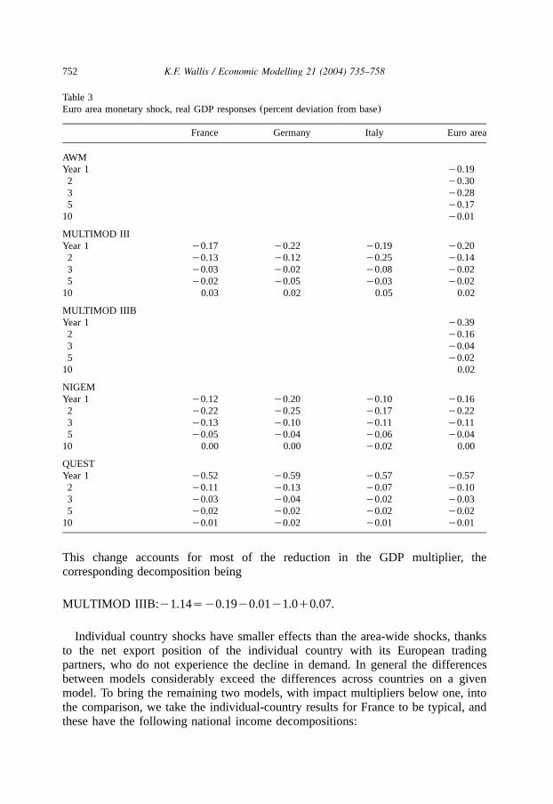
Table 3Euro area monetary shock, real GDP responses(percent deviation from base)


AWMYear 1 y0.192 y0.303 y0.285 y0.1710 y0.01

MULTIMOD IIIYear 1 y0.17 y0.22 y0.19 y0.202 y0.13 y0.12 y0.25 y0.143 y0.03 y0.02 y0.08 y0.025 y0.02 y0.05 y0.03 y0.0210 0.03 0.02 0.05 0.02

MULTIMOD IIIBYear 1 y0.392 y0.163 y0.045 y0.0210 0.02

NIGEMYear 1 y0.12 y0.20 y0.10 y0.162 y0.22 y0.25 y0.17 y0.223 y0.13 y0.10 y0.11 y0.115 y0.05 y0.04 y0.06 y0.0410 0.00 0.00 y0.02 0.00

QUESTYear 1 y0.52 y0.59 y0.57 y0.572 y0.11 y0.13 y0.07 y0.103 y0.03 y0.04 y0.02 y0.035 y0.02 y0.02 y0.02 y0.0210 y0.01 y0.02 y0.01 y0.01

This change accounts for most of the reduction in the GDP multiplier, thecorresponding decomposition being

MULTIMOD IIIB: y1.14sy0.19y0.01y1.0q0.07.

Individual country shocks have smaller effects than the area-wide shocks, thanksto the net export position of the individual country with its European tradingpartners, who do not experience the decline in demand. In general the differencesbetween models considerably exceed the differences across countries on a givenmodel. To bring the remaining two models, with impact multipliers below one, intothe comparison, we take the individual-country results for France to be typical, andthese have the following national income decompositions:


Table 4Euro area monetary shock, inflation responses(percent deviation from base)


AWM (CED)Year 1 y0.032 y0.023 y0.065 y0.1310 y0.03

MULTIMOD III (PGDP)Year 1 y0.20 y0.17 y0.25 y0.212 y0.23 y0.20 y0.25 y0.233 y0.21 y0.18 y0.21 y0.195 y0.10 y0.12 y0.09 y0.1010 0.02 0.00 0.02 0.01

MULTIMOD IIIB (PGDP)Year 1 y0.122 y0.203 y0.095 y0.0910 0.00

NIGEM (CED)Year 1 y0.04 y0.02 y0.032 0.00 y0.07 y0.023 y0.03 y0.10 y0.035 y0.03 y0.01 y0.0210 0.00 0.01 0.00

QUEST(PGDP)Year 1 y0.18 y0.17 y0.19 y0.182 y0.11 y0.10 y0.11 y0.113 0.01 0.00 0.00 0.015 0.00 0.00 0.00 0.0010 0.00 0.00 0.00 0.00

MULTIMOD:y1.26sy0.51q0.00y1.00q0.25

NIGEM:y0.78sy0.04y0.35y1.00q0.61

QUEST:y0.87sy0.09q0.08y0.97q0.12.

Model features discussed in the previous paragraph maintain their relevance. Theshare of liquidity constrained consumers falls from 0.44 in MULTIMOD Mark IIIBto 0.3 in QUEST, while NIGEM’s consumers are entirely forward-looking. Invest-ment in NIGEM is treated in a similar way to AWM, and is mainly affected throughthe demand channel, as its cost of capital measure is based on the long-term realrate of interest, which rises by a smaller amountceteris paribus than the short rateused in AWM. The fiscal shock in QUEST is a proportionate reduction in government


purchases and government employment, the latter resulting in a sharper rise in theunemployment rate than elsewhere. This has a negative impact on real wage costs,and while expected future profitability is little affected by this temporary shock, asin MULTIMOD, the change in current profitability induces a small investmentresponse of the opposite sign to that observed in other models.Cross-country differences are greatest in NIGEM. Differences in trade shares and

factor shares are reflected in all models, but NIGEM has greater variety in estimatedcoefficients across countries, in trade and factor demand equations. Its consumptionfunction is the same across the three countries in our tables, however. Here differentconsumption responses occur as different income effects induced elsewhere in themodel work through in the four quarters of the first year. They are nevertheless thesmallest consumption responses across the models, for the reason noted above.Once the perturbation is removed policy reaction functions come into play to

correct the imbalances that have arisen. Tax rates fall in response to the budgetsurplus produced by the fiscal contraction, and interest rates fall by amountsproportional to the accompanying deflation. These latter effects are greater in AWMand MULTIMOD than in NIGEM and QUEST. Again, however, MULTIMOD IIIB’smore recent estimates deliver smaller effects and hence smaller policy responses, inthis case due to the reduction in the persistence of inflation implied by reestimationof its Phillips curve on more recent data. In general adjustment occurs quickly, andtargets and instruments are back at base well within the period covered by ourtables. In NIGEM and QUEST, whose Taylor rules are forward-looking(‘inflation-forecast’ targeting), adjustment occurs with a small amount of overshooting. Theexception is AWM, whose inflation correction is much more protracted, in theabsence of forward-looking behaviour in wage and price setting in this model. Inaddition, the response of prices to the output gap is weaker in AWM than the‘marked capacity effects in the price system’ of NIGEM.

3.3. Monetary policy simulation results

Responses to the temporary increase in interest rates in the euro area aresummarised in Tables 3 and 4. Exchange rate effects are stronger in this experimentthan in the case of a worldwide increase in interest rates, and our comparativeanalysis focuses on the euro area increase.The first-year monetary policy multipliers are greater in QUEST than in the other

three models, and across countries are greater in Germany than elsewhere. In bothdimensions it is the investment response that provides the main explanation forthese differences. The direct shock to interest rates serves to emphasise modeldifferences in the treatment of investment already noted above. Although MULTI-MOD and QUEST are both based on Tobin’sq model of intertemporally optimisingfirms, in MULTIMOD changes inq have both current and lagged effects oninvestment, with coefficients 0.03 and 0.05, respectively. Since this is an annualmodel, the larger lagged effect does not feature during the period of the interestrate increase. The new estimates incorporated in MULTIMOD Mark IIIB include adoubling of the contemporaneous coefficient. These coefficient differences explain


the difference in the investment response between the two versions of the model,and help to bring the overall GDP response of Mark IIIB to a value intermediatebetween those of MULTIMOD Mark III and QUEST. The contribution of investmentto the first-year GDP multiplier in AWM and NIGEM lies between that of the othermodels; they take similar approaches to one another, with NIGEM’s smallerresponses again being explained by the use of the long-term rather than the short-term interest rate in calculating the user cost of capital. Across countries, the largerresponses in Germany are mostly due to its larger share of investment in GDP.The contribution of net exports to the first-year GDP multiplier is generally small,

although this temporary shock has a permanent effect on the nominal exchange rate.The effects are largest in AWM, albeit subject to the previous reservation about theinclusion of intra-area trade. Although the remaining contributions are small thereis disagreement about their sign, but we note that the net effect is the differencebetween two much larger quantities, each susceptible to small variations in estimatedincome and price elasticities.In the second year the setting of interest rates is determined by the monetary

policy reaction function, and fiscal policy now reacts to the deterioration in thepublic finances that has resulted from the temporary increase in interest rates. Thisincreases the cost of debt service, the more so in Italy given its larger stock ofpublic debt. In MULTIMOD the fiscal correction works mostly through householddisposable income and hence the consumption of the large share of liquidity-constrained households in this model, and the further decline in consumption issufficient to give a further decline in the overall GDP multiplier. This does notoccur in the other countries, however, and the Italian second-year decline washesout in the euro area aggregate. In contrast, AWM and NIGEM exhibit similaradditional falls in the GDP multiplier, for the area-wide aggregate in AWM, and forthe three major economies in NIGEM. A further decline in investment drives thisresult in NIGEM, indeed the second-year(negative) investment responses are largerthan the first, due again to the demand channel. AWM experiences further falls inboth consumption and investment, through the same mechanism. Finally, in completecontrast, the large first-year GDP effects in QUEST decline quickly and smoothlyback to base, reflecting its emphasis on optimising behaviour rather than estimateddynamics.Interest rate trajectories in general show the similarities to be expected from the

use of the same reaction coefficients in the Taylor rule representation of the singlemonetary policy, although in implementation there are some differences in thetiming of the inflation response, as noted above. These are sufficient to explainvariations in the size of the reduction in interest rates in the second year, relative tothe different inflation responses to the shock. Interest rates, along with inflation,then return smoothly back to base. The exception is again AWM, where theinflationary consequences are rather small but the output gap effects rather long-lived, and interest rates continue to decline for a further 3 years. In this model theinvestment responses to both shocks are very persistent and oscillatory, and raise aquestion about its dynamic specification.


4. Conclusion

The comparisons reported in this article represent a noteworthy beginning tocomparative modelling research in the new, and still evolving, economic andpolitical environment of Europe. The simulation results quantify some importantpolicy responses, and highlight some areas of the models where lack of agreementhas important consequences for these point estimates, although perhaps alsoindicating a range of uncertainty around them. Nevertheless the extent of disagree-ment is much less than in some previous model comparison projects.With monetary policy taking an area-wide perspective, an aggregate area-wide

model appears to be adequate for monetary policy making. Analysis of itsconsequences is undertaken by national central banks, however, and fiscal policyremains at the national level, albeit increasingly coordinated, hence multicountrymodelling remains necessary. The degree of variation across the three major euroeconomies studied in this exercise differs across the three multicountry models,which place different relative weights on theory and data in the process ofquantification. It is easy to surmise that, however large or small it is in this exercise,cross-country variation would be increased by including the smaller euro economies.The principal source of simulation differences across the four models is the

different degree of forward-looking behaviour they incorporate in their treatment ofconsumption and investment decisions and the setting of wages and prices. Thisaffects not only the dynamics of the economic responses to the policy experimentsconsidered here, but also, in some cases, their magnitude. It suggests an agenda forcomparative econometric testing, to try to answer Christ’s(1975) classic question,which (if any) are right, and to reduce the disagreements described above. In theirfinal review of models of the UK economy undertaken by the ESRC MacroeconomicModelling Bureau, the authors note that ‘Sometimes comparative testing may leadto a preferred andyor improved specification. The sensitivity of overall modelproperties can then be checked by replacing the various original specifications bythe preferred specification and observing the impact of this change on the compar-ative simulation results. Sometimes the available data cannot discriminate betweencompeting specifications, but at least the model user is then clear about where theuncertainty lies, and can base a choice on whatever other grounds may be appropriateto the particular application. This combination of simulation analysis of overallmodel properties and econometric analysis of individual model equations or groupsof equations in the context of cross-model comparisonswhasx proved to be aproductive methodological development’(Church et al., 2000). Its application tothe existing and emerging models of the European economy is an important nextstep.

Acknowledgments

The helpful comments, advice and assistance of Ray Barrell, Alistair Dieppe,Jerome Henry, Andrew Hughes Hallett, Ben Hunt, Jan in’t Veld and Susanne


Mundschenk are gratefully acknowledged. Responsibility for the contents of thisarticle and any errors therein nevertheless remains with the author.

References

Aghion, P., Howitt, P., 1994. Growth and unemployment. Rev. Econ. Stud. 61, 477–494.Balakrishnan, R., Lopez-Salido, J.D., 2002. Understanding UK inflation: the role of openness. WorkingPaper No.164, Bank of England, London.

Bardsen, G., Jansen, E.S., Nymoen, R., 2002. Testing the New Keynesian Phillips curve. Working Paper2002y05, Norges Bank, Oslo.

Barrell, R., Dury, K., Hurst, I., Pain, N., 2001. Modelling the world economy: the National InstituteGlobal Economic Model. Presented at an ENEPRI workshop on Simulation Properties of Macroecon-ometric Models, CEPII, Paris.

Barrell, R., Becker, B., Byrne, J., Gottschalk, S., Hurst, I., van Welsum, D., 2004. Macroeconomicpolicy in Europe: experiments with monetary responses and fiscal impulses. Economic Modelling,21, 877–931.

Bryant, R.C., Henderson, D.W., Holtham, G., Hooper, P., Symansky, S.A.(Eds.), 1988. EmpiricalMacroeconomics for Interdependent Economies. Brookings Institution, Washington DC.

Bryant, R.C., Hooper, P., Mann, C.L.(Eds.), 1993. Evaluating Policy Regimes: New Research inEmpirical Macroeconomics. Brookings Institution, Washington DC.

Christ, C.F., 1975. Judging the performance of econometric models of the US economy. Int. Econ. Rev.16, 54–74.

Church, K.B., Sault, J.E., Sgherri, S., Wallis, K.F., 2000. Comparative properties of models of the UKeconomy. Natl. Institute Econ. Rev. 171, 106–122.

Dieppe, A., Henry, J., 2004. The euro area viewed as a single economy: how does it respond to shocks?Econ. Modelling, 21, 833–875.

Fagan, G., Henry, J., Mestre, R., 2001. An Area-Wide Model(AWM) for the Euro Area. WorkingPaper No.42, European Central Bank, Frankfurt.

Gali, J., Gertler, M., 1999. Inflation dynamics: a structural econometric analysis. J. Monetary Econ. 44,195–222.

Gali, J., Gertler, M., Lopez-Salido, J.D., 2001. European inflation dynamics. Eur. Econ. Rev. 45,1237–1270.

Gorman, W.M., 1953. Community preference fields. Econometrica 21, 63–80.Hunt, B., Laxton, D., 2004. Some simulation properties of the major euro area economies inMULTIMOD. Economic Modelling, 21, 759–783.

Johansen, S., 1991. Estimation and hypothesis testing of cointegration vectors in Gaussian vectorautoregressive models. Econometrica 59, 1551–1580.

Joyce, M., Wren-Lewis, S., 1991. The role of the exchange rate and capacity utilisation in convergenceto the NAIRU. Econ. J. 101, 497–507.

Klein, L.R., 1946. Macroeconomics and the theory of rational behavior. Econometrica 14, 93–108.Laxton, D., Isard, P., Faruqee, H., Prasad, E., Turtelboom, B., 1998. MULTIMOD Mark III: the coredynamic and steady-state models. Occasional Paper No.164, International Monetary Fund, WashingtonDC.

Maclennan, D., Muellbauer, J., Stephens, M., 2000. Asymmetries in housing and financial marketinstitutions and EMU. In: Jenkinson, T.(Ed.), Readings in Macroeconomics. 2nd ed. OxfordUniversity Press, Oxford, pp. 74–98. Updated version of an article with the same title published inOxford Review of Economic Policy, 14(3), 54-80, Autumn 1998.

Manning, A., 1992. Productivity growth, wage setting and the equilibrium rate of unemployment.Discussion Paper No.63, Centre for Economic Performance, London School of Economics.

Mitchell, P.R., Sault, J.E., Smith, P.N., Wallis, K.F., 1998. Comparing global economic models. Econ.Modelling 15, 1–48.


Mitchell, P.R., Sault, J.E., Wallis, K.F., 2000. Fiscal policy rules in macroeconomic models: principlesand practice. Econ. Modelling 17, 171–193.

Muellbauer, J., Lattimore, R., 1995. The consumption function: a theoretical and empirical overview.In: Pesaran, M.H., Wickens, M.R.(Eds.), Handbook of Applied Econometrics. Blackwell, Oxford,pp. 221–311.

Nataf, A., 1948. Sur la possibilite de construction de certaines macromodeles. Econometrica 16,232–244.

Roeger, W., in’t Veld, J., 1997. QUEST II: a multi country business cycle and growth model. Workingpaper, European Commission DGII, Brussels.

Roeger, W., in’t Veld, J., 2004. Some selected simulation experiments with the European Commission’sQUEST model. Econ. Modelling, 21, 785–832.

Rudd, J., Whelan, K., 2001. New tests of the New-Keynesian Phillips curve. Finance and EconomicsDiscussion Series, Paper No.2001-30, Federal Reserve Board, Washington DC.

Rudd, J., Whelan, K., 2002. Does the labor share of income drive inflation? Finance and EconomicsDiscussion Series, Paper No.2002-30, Federal Reserve Board, Washington DC.

Sgherri, S., 2000. When is labour market flexibility welcome? More on asymmetric policy impacts inEurope. Research Memorandum WO and E No.619, De Nederlandsche Bank, Amsterdam.

Stoker, T.M., 1986. Simple tests of distributional effects on macroeconomic equations. J. Polit. Econ.94, 763–795.

Theil, H., 1954. Linear Aggregation of Economic Relations. North-Holland, Amsterdam.Turner, D.S., 1991. The determinants of the NAIRU response in simulations on the Treasury model.Oxf. Bull. Econ. Stat. 53, 225–242.

Wallis, K.F., 2000. Macroeconometric modelling. In: Gudmundsson, M., Herbertsson, T.T., Zoega, G.(Eds.), Macroeconomic Policy: Iceland in an Era of Global Integration. University of Iceland Press,Reykjavik, pp. 399–414.

Comparing empirical models of the euro economy - …€¦ · · 2006-11-14Comparing empirical...

Documents

Transcript of Comparing empirical models of the euro economy - …€¦ · · 2006-11-14Comparing empirical...