End-of-Degree paper

Comparative Effectiveness of the ARMA-GARCH

over Simple Strategies

Prepared by Ricardo Sans Cipollitti

Supervised by Christian Timothy Brownlees AY 2019-2020

Project code: EWI14

1

Table of Contents 1. Motivation ..................................................................................................... 2

2. Introduction .................................................................................................. 2

3. In Pursuit of Alpha ...................................................................................... 4

3.1. The Efficient Market Hypothesis ......................................................................... 4

3.2. Criticisms of the EMH ............................................................................................ 6

4. Analytical methods ...................................................................................... 8

4.1. Technical Analysis ................................................................................................... 9

4.2. Fundamental Analysis ......................................................................................... 10

4.3. Quantitative Analysis .......................................................................................... 11

5. Review of concepts ...................................................................................... 12

5.1. Background ............................................................................................................ 12

5.2. The ARMA Model .................................................................................................. 13

5.3. The GARCH Model ............................................................................................... 14

5.4. The combination of both ..................................................................................... 14

5.5. Comparative Simple Strategies ........................................................................ 15 5.5.1 The 200-Moving Average Strategy .................................................................................. 15 5.5.2 The Relative Strength Index Strategy ............................................................................. 15 5.5.3 The Buy-and-Hold and Random Strategies .................................................................... 16

5.6. The Studied Securities ........................................................................................ 16

5.7. The Recession Component ................................................................................. 17

5.8. Limitations of this project .................................................................................. 17

6. Empirical and Descriptive Research ...................................................... 18

7. Conclusion ................................................................................................... 21

8. References .................................................................................................... 23

9. Annex ............................................................................................................ 25

2

1. Motivation

This End-of-Degree project is intended to assess if the combination of two different statistical models —ARMA and GARCH— can perform better than the common buy and hold strategy, as well as other simple strategies. There are two different reasons for me to write this paper. The first of them is an academic motivation to apply the studies carried out in a particular course I enrolled in, Forecasting

Techniques, and test the accuracy of the models learned in the field of Finance. The second is a personal motivation to deep into the financial markets and assess the difficultness of investing in them. The project as such will firstly consist of an introduction where we will debate opposed ideas on the notion of the Efficient Market Hypothesis, then we will discuss the different types of existing analytical methods for understanding and investing in those markets and, finally, we will delve into the empirical part, where we will be using R to test the performance of all the models. In the end, we will have enough proofs to ascertain that the ARMA-GARCH outperforms the rest, yet there will be some caveats to it.

2. Introduction

In any Introduction to Macroeconomics book for first year students one can read that citizens split their money into two: consumption and investment. In the case of the latter, capital is allocated somewhere in the market. Banks, sovereign debt, housing market and others are examples of places where that money can be deposited. Certainly, those willing to refuse today’s consumption and save expect rewards in the future —in the form of interests— and thus will consider several proposals before any decision is made. Either because there is a specific company performing particularly well, because there is a technological advancement that can change the world we live in or because of any other particular reason; savers may put their and other people’s wealth in the financial markets. Once that choice is made, there is only one objective: that of making more money. However, the path to follow is not easy and risk is always present, factor that can

3

work for —but especially against— their target. Consequently, it stands to reason to find for confirmation signals which guarantee it will not affect them in a detrimental manner, giving rise to sensible investigations. The first documented behavioral finance study dates from the 17th century, Confusión de Confusiones, written by the merchant José de la Vega, book in which he depicts the complexity of Amsterdam’s Stock Exchange with trading operations and investors’ way of thinking (Corzo, Prat, and Vaquero 2014). Since then, several researchers have sought to find mechanisms that could predict traders’ behavior to stay ahead of the curve and make profits. These analyses are not easy to build and naturally, once several people know their existence, they lose power and become worthless. We will review three main types of analysis —fundamental, technical and quantitative. After classifying them, we will proceed to discuss the main hypothesis of the paper: the comparative effectiveness of ARMA-GARCH over simple strategies. The empirical project of this paper will assess the daily predictions of three different models —ARMA-GARCH, 200-day moving average and relative strength index— throughout several years for different securities1, and will discriminate if any specific model performs better under economic recession environments or not. Ultimately, these will be compared to a threshold: the buy-and-hold strategy. For that, we will first explain the purpose and objective of each of them and then we will go step by step in the development of our ARMA-GARCH. All these models will be manually coded in R and will be shown later in the annex. Finally, we will dedicate some pages to discuss the findings and accept or reject our hypothesis. However, before writing about the previous topics, it is important to introduce some notions with which the reader should be familiar. There is no academic

1 Throughout this paper, whenever the author refers to “securities”, he is referring to the set of stocks, indices, currencies, forwards, futures and all the other tradable goods available in the financial markets.

4

consensus on whether markets are, by definition, unpredictable or, on the contrary, they present small opportunities in which skilled investors can profit from arbitrage or reduced risk. This debate is crucial to the study of this hypothesis and hence the following lines will develop further on both theories.

3. In Pursuit of Alpha

3.1. The Efficient Market Hypothesis

Some academics like Eugene E. Fama (1970) claim that prices fully reflect all available information, implying that it is impossible to beat an efficient market with an active management strategy, this consisting of exploiting miscalculated assets on a risk-adjusted basis (Ang, Goetzmann, and Schaefer 2011). Other implications are that short-term price changes are independent and identically distributed, forming a random walk model. The paper further discusses the market efficiency by dividing the concept of information into three: weak, semi-

strong and strong forms. In its weak form, the only information available in the market is that of historical prices, and this can be predicted with trends. The semi-

strong form concerns all publicly-available information, like financial news, business annual reports and announcements, which naturally can be accessed by anyone. Lastly, the strong form involves those agents who have privileged information with respect to other investors, with a particular emphasis on mutual funds. Although he mentions that there is evidence of some specialists in the NYSE using their monopolistic access to generate profits, a research conducted by M. Jensen (1968), in which he studied the returns of 115 mutual funds over a period of 10 years, supports Fama’s main thesis: 89 out of 115 funds were still below the market. Moreover, even when loading charges were not taken into account, i.e., salesman commissions, 72 out of 115 funds were still below the market line, with almost 9 percent deviation in that period. Another supporter of the EMH is B. Malkiel, author of several books and articles related to this topic. In one of his most notable books, A Random Walk Down Wall

5

Street (1973), he compares different types of models and concludes that, on a long-term basis, no active management can beat the market. He quotes in that book (p. 24):

“A blindfolded monkey throwing darts at a newspaper’s financial pages could select a

portfolio that would do just as well as one carefully selected by experts”

Besides, he also endorses the study made by Jensen as he detects that the average annual rate return over 10 years for general equity funds in 1998 was +15.24 percent vs. +18.56 percent made by the S&P500 at that time. Another intriguing fact was that the 20 best-performing equity funds in the period of 1970-80 had an average annual return which almost doubled the average of all 177 funds studied, whereas those same 20 underperformed the average in the subsequent period 1980-90 (+11.1 percent against +11.7 percent respectively), thus suggesting the idea that mutual funds tend to regress towards the mean. In his article The Efficient Market Hypothesis and Its Critics, Malkiel (1979) studied several attacks to the concept of market efficiency —understood as the impossibility to earn above-average returns without incurring into higher risk— and claimed that, although there have been some periods in history where investors did not trade rationally, markets can still be efficient. Those seemingly-irrefutable periods of inefficiency included the market crash of October 1987 and the internet bubble of the late 1990s. For the first case, two months before the collapse, yields on long-term US Treasury bonds increased from 9 to 10.5 percent, the US Secretary of the Treasury threatened to lower the USD exchange rate, and the US Congress raised the idea of imposing a merger tax, possibly damaging the merger boom of that period. For the second case, all types of financial experts were overestimating equity valuations for high-tech and telecommunication companies as they were reading explosive growths for those industries. However, with the benefit of hindsight, we now know that those projected rates were unsustainable. Certainly, these factors were not the only trigger for the abnormal events, yet they prove the fact that there was a rational argument behind, therefore upholding the idea of efficiency.

6

3.2. Criticisms of the EMH

On the other hand, some investors and researchers oppose the EMH. Warren Buffett, for his part, criticized those in favor of EMH on a speech he gave at Columbia Business School in 1984. He asked the audience to imagine 225 million Americans tossing a coin once every day and trading bullish or bearish according to the results. After twenty days, roughly 215 people would correctly guess market behavior. Some Business professors, he added, would argue that that is pure statistics, so 225 million orangutans dispersed around the US could have had the same outcome. However, Buffett expressed that that would not be true if 40 of those 215 orangutans lived in the same place: “Graham-and-Doddsville”, referring to 40 successful investors that traded different securities but followed the same foundations: the teachings of professors Graham and Dodd (Buffett 1984). That true fact served Buffett to shatter the EMH theories of his rival speaker, the aforementioned prof. Jensen. In fact, Seth Klarman (1991) —American investor and hedge fund manager— stated in his book Risk-Averse Value Investing

Strategies for the Thoughtful Investor (p. 99):

“Buffett's argument has never, to my knowledge, been addressed by the efficient-market

theorists; they evidently prefer to continue to prove in theory what was refuted in

practice”

Some researchers have also had the opportunity to disapprove the EMH. Critics are varied and can be classified into supporters of short-term momentum, long-run return reversal and seasonal and day-of-the week patterns (Malkiel 1979). We proceed to describe these positions in the following lines. Lo and MacKinlay (1987) studied the randomness of numerous financial instruments from 1962 to 1985 as well as for smaller periods, concluding that weekly and monthly holding-period returns had significant positive autocorrelation implying some momentum in short-term periods and also rejecting the idea that security returns behave like random walks. Furthermore, Lo and Wang (2000) later described the foundations of technical analysis and how to

7

assess its effectiveness by implementing an automatic approach to technical pattern detection using nonparametric kernel regressions and then applying them to several securities in the US from 1962 to 1996, leading to the conclussion that some basic indicators such as the double-bottoms and head-and-shoulders were useful for finding predictive patterns and again, rejecting the idea that markets are efficient. While in the short-term it seems that financial instruments’ returns follow a positive autocorrelation, the opposite happens in the long term. According to W. De Bondt and R. Thaler (1985), extreme movements in security prices are followed by price movements in the opposite direction, thus suggesting negative serial correlation. This market overreaction is also supported by founders of the prospect theory D. Kahneman and A. Tversky (1977) in their article Intuitive Prediction:

Biases and corrective procedures decision, as they suggest that judgements tend to match the impression of people rather than the objective past experiences. The following example from their article illustrates this rule:

“An editor reviewed the manuscript of a novel and was favorably impressed. He

said: ‘This book reads like a best-seller. Among the books of this type that were

published in recent years, I would say that only one in twenty impressed me

more’. If the editor were now asked to estimate the sales of this novel, he would

probably predict that it will be in the top 5 percent of the distribution of sales.”

In case of perfect predictability, i.e., the editor knows with certainty that the book will be in the top 5 percent sales, then assumptions match predictions. However, when there is no certainty, which is the most common, the editor should not trust his assumption that much: he should better trust previous outcomes. Same happens with financial markets. When an extreme event occurs, investors tend to forget past returns and focus on the current situation, following herd behaviors, until they reach a point where they realize that previous data matters more, thus returning to more fundamental values, i.e., mean reversion.

8

Finally, some researchers have studied that the month of the year or the day of the week can affect security markets. M. Rozeff and W. Kinney (1976) considered month returns from an equal-weighted index of NYSE from 1904 to 1974 and concluded that there were statistically significant seasonal patterns. More specifically, January seemed to have around +3.5 percent return whereas the rest of the months averaged +0.5 percent. Similarly, French (1980) assessed the importance of each workday of the week from 1953 through 1977 and ascertained that the mass for Mondays’ returns histogram was mostly in the negative region, while the other four days of the week presented more symmetric shapes. All in all, we can clearly see two opposed views on this topic. Some academics find impossible to make alpha whereas others argue that it is possible under certain circumstances. As detailed by Malkiel, although there are some rational factors involved in specific recessions, psychological factors also play a role in market performance. Furthermore, W. De Bondt and R. Thaler also mention that extreme movements tend to return to a fairer price after some time —when investors start looking back at numbers instead of following herd behavior. These findings pave the way for making the following questions: is it possible that a combination of two statistical models can outperform the market? Is it possible that they perform better than a buy-and-hold strategy in recession periods? Can they perform better than other models? These are all questions that will be answered in the following pages. Notwithstanding, before we test the hypotheses, we will discuss about the different types of analytical methods used nowadays, important for understanding the foundations to all of our strategies.

4. Analytical methods

In the previous section we have seen the EMH and its critics. Now we will briefly examine different types of analysis for market price forecasting, relevant for the study of our hypothesis, as assuming that there is only one way to predict the prices of financial instruments would lead inconsistencies in the final conclusion

9

of this paper. There is little consensus in the research literature on the specific number of predicting methods, so we will divide them into technical, fundamental and quantitative.

4.1. Technical Analysis

In his weak form of information, Fama claimed that in an efficient market upcoming prices could not be predicted with historical data. However, technical analysis aims at predicting prices with the same arguments that Fama said were not possible. The fashion in which security prices move along a time series might be indicators of market trends, consequently showing predictive signals. This study therefore believes that the future is —and will keep being— a copy of the past.

“I believe the future is only the past again, entered through another gate”

—Sir Arthur Wing Pinero, 1893

The first application of this analysis was made by Wall Street Journal cofounder, Henry Dow. During his life he wrote several articles related to financial markets and created the first stock market index —the Dow Jones Transportation Average. After his death, A. J. Nelson, W. P. Hamilton and R. Rhea compiled pieces of Dow’s researches (Schannep 2012) and called them the Dow Theory. In these articles they exposed Dow’s main theories on the stock market, which are still used by many technical analysts nowadays. We shall not dive deep into all of the theorems, though we will consider the notions of one of them —trends— as they are the gateway to two of the simple strategies used to assess the efficiency of the ARMA-GARCH model: the simple moving average and the relative strength index (RSI). In one of the rewritten versions of the Dow’s theorems, R. Rhea describes that there are three Dow movements: the primary trend, the secondary reaction and the daily fluctuations. In the primary trend, broad momentum of market prices leads the way for future values. They can be bullish —indicating an upward trend— or bearish —downward trend—, and extend over periods from months to several years. The secondary reaction is the opposed drift that the market

10

experiences when in a bullish or bearish trend. It can or cannot represent a change in the primary trend, but certainly all changes in trend start with a secondary reaction, and can last from three to several months. The third movement are the daily fluctuations, almost always meaningless price movements that provide little information and can sometimes be confusing. In the next chapter we will understand how this concept of trend and its different movements shape the idea of the 200-days moving average and the RSI.

4.2. Fundamental Analysis

If technical analysts look for patterns in historical prices, fundamental analysts are constantly seeking for undervalued and overvalued securities in hopes that their prices will correct over time. This type of analysis is based on three main pillars (Hu et al. 2015) briefly described below. The first pillar to be studied is macroeconomic analysis, which analyzes the global monetary and fiscal measures, inflation, unemployment and GDP trends. They are crucial for the study of foreign exchange rate, bond and stock markets. The second pillar is the industrial analysis, which examines the overall performance of any given industry by reading and judging top businesses’ annual reports. They are useful for predicting the general trend and potentiality of the industry and, in essence, the traded stock. The third and last pillar is the company analysis, which explores the current operation status of the businesses whose stock will be traded, as well as their credibility, to assess their fair value and trade accordingly. Again, in this case, the source of information comes from financial reports. Renown fundamental analysts include the aforementioned Warren Buffett and his instructor, Benjamin Graham. They not only beat the EMH several times, but also defended that fundamental analysis was much more profitable than technical analysis. In Berkshire-Hathaway’s annual letter for 2016, Buffett praised those who invested in the S&P500 based on a sensible and fundamental analysis and

11

kept a buy and hold position, since he defends Malkiel’s point of view that mutual and hedge funds’ commissions consume potential profits. Similar to section 4.1., the buy and hold strategy what we will be using for our comparison can be classified as part of the fundamental analysis and will be further discussed in the following chapter.

4.3. Quantitative Analysis

Quantitative analysis is “the trading of securities based strictly on the buy/sell decisions of computer algorithms” (Chan 2009). It is similar to technical analysis as it also considers information given by previous data, yet they differ in that the final decision of this one is given by a computer based on a trading algorithm rather than on human interpretation. Moreover, quantitative analysis might also integrate some aspects of fundamental analysis such as P/E ratios and interest rates. As long as this information can be filtered into numbers, it can be an additional and useful resource for price forecasting. For any analysis to be considered as quantitative, five requirements are needed (Guo et al. 2016): data, models, analytics, algorithms and optimization. The first one, data, is the cornerstone for building a study of such characteristics. Stock prices, quarterly GDP, annualized CPI, liquidity ratios and seasonal revenues are only a few examples of data that investors can retrieve —free of charge in most of the cases— and use them for their own trading purposes. Models are the linkage between the data and the computer decision, so we could argue that if data were the foundations of a building, models would be the beams and bricks. Analytics entails the way we look at raw numbers and use them for the development of data-driven strategies. Algorithms are instructions aimed at calculating solutions for our mathematical problems by using a computer language. The use of variables, conditional statements and for loops can be considered examples of an algorithm. Finally, the responsibility of throwing the best outcome depends on the optimization problem we suggest to the model. For instance, if we want to draw a linear regression in order to provide the best fit to some data, possible optimizers

12

for this model could be the Ordinary Least Squares or the Generalized Least

Squares, among others. The application of quantitative analysis in markets is usually more complex than the previous two, as the science behind it not only requires business and economic knowledge, but also a reasonably high mathematical, statistical and programming background. One of the greatest exponents of this analysis is high-frequency trading, also known as HFT. It uses super-efficient computer languages, like C++ or Java, combined with complex algorithms and connected to global markets, ready to trade, in a matter of milliseconds, thousands of securities. Naturally, there are other implementations that do not need super-fast programming languages and can run in a slower manner for those seeking non millisecond-trading strategies, like in our case with the ARMA-GARCH. We can sum up saying that technical analysis uses the weak form, fundamental analysis uses a semi-strong form and quantitative analysis uses both a weak and semi-strong forms of information for casting a decision. Moreover, we have introduced the founding stones for what they would be all of our used strategies: the moving average, the RSI, the buy-and-hold and the ARMA+GARCH. The choice of analysis depends on the knowledge, resources and beliefs available to the person concerned. Since all of them have their ups and downs, they are usually combined to take the best conclusions from different points of view. It is important to highlight this fact as, in this paper, only a quantitative approach will be considered.

5. Formalization of concepts

5.1. Background

Although the autoregressive moving average process (ARMA) was firstly described in Peter Whittle’s (1951) thesis, it was not until 1970 that Box et al. popularized this model by taking the first difference of IBM’s stock prices and, after taking its

13

logarithm, computed the moving average (MA), autoregressive (AR) and ARMA processes based on the results of the autocorrelation (ACF) and partial auto correlation (PACF) functions in order to predict its future value. That same year, Box and Pierce introduced a test that could assess the suitability of an ARMA model on any given time series, although subsequent simulations proved poor performance. Finally, Ljung and Box (1978) took that previous model and modified it until they finally found an appropriate formula. This test —the Ljung-Box test— measures the autocorrelation found in the residuals after an ARMA model has been fitted in the data. If the residuals are white noise, the null is not rejected, otherwise, it is. After these findings, however, there was still one question to be solved. When fitting ARMA models to financial time series, some residuals follow conditional volatility —mainly due to great unexpected events— which the model is not able to capture. For this reason, Engle (1982) developed the Autoregressive Conditional Heteroskedasticity (ARCH), a model that can reduce non-stationary residuals into stationary using a sequence of differencing steps. Engle’s doctoral student, Tim Bollerslev (1986), enhanced the ARCH model and converted it into the Generalized Autoregressive Conditional Heteroskedasticity (GARCH) model. In the following lines we will proceed with theoretical framework of the models introduced in this paper. First, we will consolidate the definition of the ARMA-GARCH, as well as the other models: 200-days moving average and relative strength index. Finally, we will compare all of them to our benchmark, the buy-and-hold strategy. Our objective is to see whether the ARMA-GARCH performs better than the other strategies throughout some specific period intervals and under recession periods.

5.2. The ARMA Model

The ARMA(p, q) is a linear model based on two other linear models: the AR and the MA. It follows this expression:

14

𝑦! =𝑐 + 𝜙"𝑦!#" +⋯+𝜙$𝑦!#$ + 𝜀! +𝜃"𝜀!#" +⋯+ 𝜃%𝜀!#% ,𝑤ℎ𝑒𝑟𝑒𝜀!~𝑊𝑁(0, 𝜎&')

One of the main features of the ARMA is that it is parsimonious and redundant in its parameters. That is, an ARMA model will often require fewer parameters than an AR(p) or MA(q) model alone, which improves the chances of overfitting our model. A pure ARMA model draws several characteristics mentioned in the following lines. Its correlogram should decay exponentially for both the ACF and the PACF since this model integrates the features of the AR and MA model, i.e., we have both direct and indirect effects of past values at 𝑡 + 0.

5.3. The GARCH Model

As mentioned in the background chapter of this section, the GARCH model aims at capturing the volatility that the ARMA cannot. This model is carried out because financial data does not have a constant variance across time but instead shows signs of volatility clustering, i.e., large returns —in absolute value— tend to be followed by large returns —in absolute value as well—, and vice versa. Therefore, we need a formula that can capture this variability according to past volatility:

𝜀! = 𝜎!𝑧! ,𝑤ℎ𝑒𝑟𝑒𝑧~𝑊𝑁(0,1)

𝜎!' = 𝛼( +:𝛼)𝜀!#)' +:𝛽*𝜎!#*'

$

*+"

%

)+"

As we can observe, the GARCH(p, q) model depends on past white noise and volatility. One of the advantages of using this model over its more old-fashioned version —the ARCH(p)— is that it can be proven that it is more parsimonious and thus less prone to overfit.

5.4. The combination of both

For the purpose of implementing a good fit to our financial data, we will propose a hybrid combination of both models to get the best out of them. There will be two

15

stages in its implementation. In the first stage, we will fit an ARIMA(p, 1, q), i.e., an ARMA(p, q) on first-differenced data. The best-suited ARIMA is used to model the linear component of our time series, with some subsequent residuals that represent the non-linear data. In the second stage, the GARCH will be used to model those non-linear components of the residuals.

5.5. Comparative Simple Strategies

5.5.1 The 200-Moving Average Strategy

As mentioned in section 4.1. of this paper, the 200-days moving average strategy (200-MA) is commonly used among those who base their trade in a more technical analysis. It provides the trader with useful information regarding the long-run trend of the market. If prices are constantly above the MA it means that the market is following a bullish trend, whereas if prices are below, then it is a bearish trend. Therefore, whenever we will be coding the daily action of this strategy, we will assign a value of 1 —or buy— when market is bullish and -1 —or sell— when market is bearish. Furthermore, we will use a 200-days MA, which means that the value of the strategy on any given day represents the simple mean of the past 200 days.

5.5.2 The Relative Strength Index Strategy

The relative strength index (RSI) was developed by J. Wilder in 1978 and is also considered to be another tool in technical analysis. It consists of a formula that is negatively affected by bull sessions and positively affected by bear sessions, all of them limited to a certain period. That is, if we choose a 10-day period, then the formula will only consider bullish and bearish sessions out of those 10 days. This function will always return a value between 0 and 100. If the RSI is close to 100 it means that the market is in upward trend for a long time and perhaps it will lose trend power in a near future, while values close to 0 mean exactly the opposite. According to its originator, the RSI is best-suited with periods of 14 days with 30 and 70 as their lower and upper thresholds, respectively. This means that once those boundaries are surpassed, a buy or sell order, respectively, should be placed.

16

5.5.3 The Buy-and-Hold and Random Strategies

In order to have a better understanding on how well our strategies will perform, we will set an upper and lower threshold to them. The upper threshold will be the buy-and-hold strategy. As aforementioned, this methodology is widely used by a considerable number of fundamental analysts that aim at making profits on a long-term basis. This strategy was originally conceived as one in which we buy a number of securities in one specific day and then let them grow until we consider they are mature enough. However, for the purpose of homogenizing the basic structure of all strategies, this time we will place daily buying orders. At the same time, as the lower threshold, we will conduct a confusion matrix for assessing their performance and will check their accuracy, i.e.:

𝐴𝑐𝑐. = 𝑡𝑟𝑢𝑒𝑝𝑜𝑠𝑖𝑡𝑖𝑣𝑒𝑠 + 𝑡𝑟𝑢𝑒𝑛𝑒𝑔𝑎𝑡𝑖𝑣𝑒𝑠

𝑡𝑟𝑢𝑒𝑝𝑜𝑠𝑖𝑡𝑖𝑣𝑒𝑠 + 𝑓𝑎𝑙𝑠𝑒𝑝𝑜𝑠𝑖𝑡𝑖𝑣𝑒𝑠 + 𝑡𝑟𝑢𝑒𝑛𝑒𝑔𝑎𝑡𝑖𝑣𝑒𝑠 + 𝑓𝑎𝑙𝑠𝑒𝑛𝑒𝑔𝑎𝑡𝑖𝑣𝑒𝑠

It will be helpful for understanding if any given model has more than 50% accuracy, which will mean that they can beat —on average— a random strategy and thus have predictive power. We will also compute its lower and upper 95% confidence intervals as a double-check.

5.6. The Securities Studied

Although the empirical research shown in the annex only shows the S&P 500 index approach, other securities are also studied following the same methodology in order to attain more observations and a more solid conclusion. Inside the realm of indices, the S&P 500 (^GSPC), Nikkei 225 (^N225), DAX 30 (^GDAXI), FTSE 100 (^FTSE) and the Hang Seng 50 (^HSI) will be considered. For the group of equities, these will be Coca-Cola (KO), Amazon Corp. (AMZN), Daimler AG (DAI.DE), Microsoft (MSFT) and Santander (SAN). Finally, the currency pairs to be studied will be EUR/USD, USD/JPY, EUR/GBP, AUD/CAD and GBP/CHF. The periods from which these securities will be studied will coincide with the beginning of the “youngest” of the category, so that all of them contain non-NA values.

17

Therefore, for the indices, we will begin from 01/12/1987; for equities, 01/05/1997; and 01/01/2003 for currency pairs.

5.7. The Recession Component

As we have discussed previously in section 3.1. Malkiel defends the idea that the human component might take part in financial markets when a recession is occurring. In order to test this hypothesis for our model, we will separate our time series into recession and non-recession periods with data provided by the Federal Reserve Bank of St. Louis. Then, we will compare the performance of all models following this split and provide a conclusion for it.

5.8. Limitations of this project

As well as with university lectures, when dealing with financial time series data and quantitative models it is usual to find some constraints that do not allow us to fully match theory with practice. In this case, there are several that we want to mention. The first, commented in the last part of section 4.3. concerns the solely application of quantitative analysis which, by itself, is not a good enough tool to provide accurate forecasting in prices. In words of Fama: “if the information contained in that record is fully reflected in today’s prices, it will be impossible to make excess profits by the use of the record”. A more thorough research should include technical and fundamental components. The second limitation is that fitting ARMA-GARCH models for time series whose length is several decades is difficult to process on today’s personal computers, so the solution we proposed to this was creating a rolling model containing only the prices of the two years prior to the predicted price instead of all the time series up until that day. We realized of the third restriction when running our code in R and this had to do with convergence. Sometimes the optimization algorithm of the package we were using did not provide a converged solution to our ARMA-GARCH model in specific days. Because of that, we decided to patch this issue by setting random orders —buying or selling— whenever that occurred. Definitely, this has no predictive power, but since it was not a frequent problem, it did not alter our results significantly. The

18

fourth regards the recession index that we were using —GDP-Based Recession Indicator Index — which is commonly used in economics. This dataset only contains US parameters and therefore is meant to be used solely for the US economy. However, since there is no global indicator, we used it in our study as a proxy. Finally, it is important to mention as the fifth limitation that this research does not take into account fees of any kind. This means that no spread in the price is assumed, as well as no entrance, overnight financing nor any other commission that might be incurred by the service provider.

6. Empirical and Descriptive Research

The following lines will guide us to the last part of this paper and will be divided into an analytical approach, where only explanatory details will be provided, and a conclusion part, where we will recover all the concepts discussed previously in this project and will combine them for the purpose of delivering a sensible answer to our hypothesis. After retrieving the time series from Yahoo Finance website and building the models in R, we processed the information for each of them—date, daily orders, daily gain/loss, etc.— and captured relevant statistics. More concisely, each security was divided into four categories: buy-and-hold, ARMA-GARCH, 200-MA and RSI. Columns were set as: days studied, cumulative return, 95% confidence interval accuracy and, for the case of the ARMA-GARCH, a mean absolute error, and rows were set as: recession, non-recession and all periods. Since it may sound confusing, Figure 3 (annex) aims at improving its comprehension. As we might remember, the objective of this project is to set a statistical foundation on whether the ARMA-GARCH can beat the other simple strategies, including the buy-and-hold. Certainly, it would make no sense if our models did not have any accuracy power, that is, we need them to predict more successful trades than unprofitable ones, which means that the computed lower 95%CI

19

accuracy parameter has to be greater than 50%. Likewise, we need our strategies to make —at least— 100% of cumulative return, i.e., we obtain the same as what we initially deposited. Because of these conditions, we shall restrain our search only to those compliant observations.

With all this in mind, we constructed the following table, shown in Figure 1, which contains the counting for those strategies that successfully met the two requirements above-mentioned. Out of 180 time series, only 35 were favorable enough. By analyzing the table, we realize that all indices were somehow well-predicted and they have a high concentration of cases —28 out of 35. Analogously, the ARMA-GARCH got the highest concentration, followed by the 200-MA and the buy-and-hold strategies. Moreover, it is important to note that, from the equity’s category, only KO

and DAI.DE attain predictive power, although their effective periods are totally different. Finally, as it can be observed on Figure 3 of the annex, applying these methodologies on the full time series dataset gives better results than only recession or non-recession periods, although SARS-CoV-2 stage might change this point of view in case the US Federal Reserve finally declares it as a recession. An example of this can be clearly seen in Figure 7, showing a great positive spike in those days for the S&P500.

Figure 1

20

After analyzing the quantitative approach, it is time to assess the qualitative one. In Figure 2 we plotted our 35 successful trades in a scatterplot with “cumulative returns” in the y axis and “lower bound accuracy” in the x axis. The purpose of it is to graphically discriminate among the best strategies. At first, we would reason that points should follow a positive correlation since the more predictive a model is, the more returns we can make. However, it is not the case. We instead observe that the highest returns belong to ARMA-GARCH models that had relatively low accuracy. whereas those with highest accuracy —mainly the RSI and 200-MA— performed with lower returns.

Figure 2

Since the ARMA-GARCH is the only model capable of casting a concise value for each prediction, we also decided to compute its MAE and compare it among the different securities. As we can see in Figure 5 (annex), it appears that for larger values of MAE the cumulative return is also larger, indicating positive correlation.

Finally, we will review a joint comparison of all the models by generating a boxplot and using the y axis for the cumulative returns, visible in Figure 6 (annex). Although the four of them seem to have a similar median, the ARMA-GARCH and buy-and-hold strategies show several outliers with relatively higher cumulative

21

returns. On the other hand, the RSI followed by the 200-MA hardly ever beat the other two.

7. Conclusion

At the very beginning of this document we studied the great controversy between those supporting the EMH and those against it. From an efficient point of view, it seemed impossible to beat the market as it contains, per se, all possible types of information available. On the other side, critics defend both the ideas that markets can be predicted when there is —and is not— a recession taking place. Examples of such figures are Warren Buffet with his Graham-and-Doddsville tale, Kahneman and Tversky exemplifying behavioural economics’ patterns, or De Bondt and Thaler proving that extreme movements in financial markets tend to return to stable and more precise prices after some time. Next, we covered the different disciplines inside the realm of financial analytics. A concise study on each of them showed us that people have at their disposal several very different tools for investing in financial markets and that these are the cornerstone for our four studied models. The technical analysis gave rise to two of them, the 200-MA and the RSI. They have in common the purpose of demonstrating to the investor the general market trend and indicating whether a security is currently undervalued or overvalued. Similarly, the fundamental analysis aims at discovering the same mismatches although the means to achieve this are different. In this case, investors follow macroeconomic trends, as well as annual reports from companies to make rational decisions. Finally, we find quantitative analytics, a technique that combines mathematical and statistical backgrounds with past price data and signals a prediction output for a specific time period. The empirical and descriptive research of this paper described several statistics that will help us finally accept or reject our hypothesis. Judging by the information given on figures 1 and 6, clearly the RSI proves to be quite an inefficient strategy

22

compared to the others. Furthermore, the ARMA-GARCH seems to be particularly suitable for indices yet not for equities nor foreign exchange markets, whereas the moving average proves somehow better results in these last two. Moreover, Figure

2 displays a nice visual scatterplot where we can clearly see that those successful strategies with the highest returns were ARMA-GARCH, followed by buy-and-hold. Nonetheless, the ARMA-GARCH is not among the best regarding the ones that evidence the highest predictive accuracy, were instead we find the RSI followed by the 200-MA. This signals that there might be a trade-off between profitability and accuracy and investors might have to take their strategy depending on their risk-aversion. Figure 5 also supports this idea, as higher returns tend to bear more error or risk. Finally, by judging Figure 6, we notice that the ARMA-GARCH presents —generally speaking— more positive outliers than the rest and it can be undoubtedly seen in action with the performance-plot for the S&P500 in Figure 7. With all this in mind, is the ARMA-GARCH better than other simple strategies? The answer is yes. With all the publicly available information that we could gather we can finally conclude that the ARMA-GARCH is a better strategy than the rest, especially when predicting indices, although it is not clear whether it performs better in adverse periods or not. We can also expose that ARMA-GARCH proves to have more risk than other strategies, such as the widely used buy-and-hold. Finally, bad news is that in real life it is hard to implement our winning strategy without incurring in daily commissions, fact that makes it a riskier and most probably unprofitable choice in the long run.

If active managers win, it has to be at the expense of other active managers. And

when you add them all up, the returns of active managers have to be literally zero,

before costs. Then after costs, it’s a big negative sign.

—Eugene E. Fama, 2014

23

8. References

Ang, Andrew, William N. Goetzmann, and Stephen M. Schaefer. 2011. 5 Foundations and Trends in Finance The Efficient Market Theory and Evidence:

Implications for Active Investment Management. Bollerslev, Tim. 1986. “Generalized Autoregressive Conditional

Heteroskedasticity.” Journal of Econometrics 31: 307–27. De Bondt, Werner F.M., and Richard Thaler. 1985. “Does the Stock Market

Overreact?” The Journal of Finance 40(3): 793–805. Box, George E. P., Gwilym M. Jenkins, Gregory C. Reinsel, and Ljung Greta M.

1970. Time Series Analysis: Forecasting and Control. 5th ed. Box, George E. P., and David A. Pierce. 1970. “Distribution of Residual

Autocorrelations in Autoregressive-Integrated Moving Average Time Series Models.” Journal of American Statistical Association 65(332): 1509–26.

Buffett, Warren E. 1984. “The Superinvestors of Graham-and-Doddsville.” Columbia Business School Magazine: 1–13.

Chan, Ernest P. 2009. Quantitative Trading: How to Build Your Own Algorithmic

Trading Business. Corzo, Teresa, Margarita Prat, and Esther Vaquero. 2014. “Behavioral Finance in

Joseph de La Vega’s Confusion de Confusiones.” Journal of Behavioral

Finance 15(4): 341–50. Engle, Robert F. 1982. “Autoregressive Conditional Heteroscedacity with

Estimates of Variance of United Kingdom Inflation.” Econometrica 50(4): 987–1008.

Fama, Eugene F. 1970. “Efficient Capital Markets: A Review of Theory and Empirical Work.” The Journal of Finance 25(2): 383–417.

French, Kenneth R. 1980. “Stock Returns and the Weekend Effect.” Journal of

Financial Economics 8: 55–69. Guo, X, Tze Leung Lai, Howard Shek, and Samuel Po-Shing Wong. 2016.

Quantitative Trading: Algorithms, Analytics, Data, Models, Optimization. Hu, Yong et al. 2015. “Application of Evolutionary Computation for Rule Discovery

in Stock Algorithmic Trading: A Literature Review.” Applied Soft Computing

24

Journal 36: 534–51. Jensen, Michael C. 1968. “Problems in the Selection of Security Portfolios - The

Performance of Mutual Funds in the Period 1945-1964.” Journal of Finance 23(2): 389–416.

Kahneman, Daniel, and Amos Tversky. 1977. “Intuitive Prediction: Biases and Corrective Procedures Decision.” Judgment under Uncertainty: Heuristics

and Biases: 414–22. Klarman, Seth. 1991. Risk-Averse Value Investing Strategies for the Thoughtful

Investor. Ljung, G. M., and G. E.P. Box. 1978. “On a Measure of Lack of Fit in Time Series

Models.” Biometrika 65(2): 297–303. Lo, Andrew W., and A. Craig MacKinlay. 1987. “Stock Market Prices Do Not

Follow Random Walks: Evidence from a Simple Specification Test.” A Non-

Random Walk Down Wall Street: 17–46. Lo, Andrew W, and Jiang Wang. 2000. “Foundations of Technical Analysis:

Computational Algorithms, Statistical Inference, and Empirical Implementation.” The Journal of Finance.

Malkiel, Burton G. 1973. A Random Walk Down Wall Street. ———. 1979. “The Efficient Market Hypothesis and Its Critic.” 17(1): 59–82. Rozeff, Michael S., and William R. Kinney. 1976. “Capital Market Seasonality: The

Case of Stock Returns.” Journal of Financial Economics 3(4): 379–402. Schannep, Jack. 2012. Dow Theory for the 21st Century Dow Theory for the 21st

Century: Technical Indicators for Improving Your Investment Result. Warren Buffet. 2017. “Berkshire-Hathaway Annual Letter 2016.” : 24–25.

http://www.berkshirehathaway.com/letters/2016ltr.pdf. Wilder, J. 1978. 24 New Concepts in Technical Trading Systems New Concepts in

Technical Trading Systems.

25

9. Annex

Figure 3

Figure 4

Figure 5

26

Figure 6

Figure 7

27

FINAL YEAR PROJECT

CODE

Comparative Effectiveness of ARMA-GARCH over Simple Strategies

Ricardo Sans Cipollitti

2020-05-31

Setting parameters part 1

# Derivative ticker as is shown in Yahoo Finance ticker = "^GSPC" # Time period of the whole dataset from = "1987-12-01" to = "2020-05-29"

Retrieving the data

# Retrieve the data mydata = as.data.frame(getSymbols(ticker,src="yahoo", auto.assign = FALSE, from = from, to = to)) # Let's observe if there is any NA in the dataset mydata %>% dplyr::mutate(date = as.Date(rownames(mydata), "%Y-%m-%d")) %>% dplyr::filter(is.na(mydata[, 6]))

## [1] GSPC.Open GSPC.High GSPC.Low GSPC.Close GSPC.Volume ## [6] GSPC.Adjusted date ## <0 rows> (or 0-length row.names)

# If there are days that might contain NA's, we will remove them later

Cleaning the data

Here we manipulate the data until we have a dataframe containing only the columns date, adjusted price and return.

mydata = mydata %>% # Inverting the dataframe dplyr::arrange(as.Date(rownames(mydata))) %>% # Setting index (date) as a column dplyr::mutate(date = as.Date(rownames(mydata), "%Y-%m-%d")) %>% # Remove holidays dplyr::mutate(adjusted = mydata[ , 6]) %>% dplyr::filter(!is.na(adjusted)) %>% # Compute the daily return and adjusted value dplyr::mutate(return = c(NA, diff(log(adjusted)))) %>% # Remove the first row containing NA in "return" dplyr::slice(2:n()) %>% # Drop unnecesary data dplyr::select(-c(colnames(mydata)[c(1:6)])) %>%

28

# Rearrange columns dplyr::select(date, adjusted, return)

Setting parameters part 2

Once we establish all the fist parameters, we proceed to adjust the amount of rolling days that we want our training model to be based on.

# Number of observations for each roll roll = 504 # Approx. 2 working years # Split date between train and test split_date = mydata[roll+1, "date"]

The training set will contain 504 observations, and we will pull new data from the test set. They will all be contained in a big list that we will create in the following lines.

Splitting into train and test

# Train set (prediction number one) train = mydata %>% dplyr::filter(date < split_date) # Test set (following predictions) test = mydata %>% dplyr::filter(date >= split_date)

Creating a rolling list whose members all contain 504 observations. Note that, for each subsequent member of the list, the first element is removed and the last one updated.

# length of the test set n = length(test$return) # Creating an empty list for filling it later roll_lists = list() # Building these rolling lists for(i in 1:n){roll_lists[[i]] = c(train$return, test$return[0:(i-1)])} for(i in 1:n){roll_lists[[i]] = tail(roll_lists[[i]], roll)} # If an error is thrown here, it probably means that the variable roll is bigger than the observations from the whole dataset, # then a bigger time period is encouraged

Making forecasts with the Rugarch package

# Designing an empty dataframe where to contain relevant variables forecast_df = data.frame(date = as.Date(n), prediction = numeric(n), action = numeric(n), return = numeric(n), gain_loss = numeric(n)) # Before predicting we will build a function to fit the optimum ARMA-GARCH model arma_garch_funct = function(index){ # Orders of the best ARMA model according to AIC orders = auto.arima(roll_lists[[index]],seasonal = FALSE, ic = "aic")$arma # Specify the type of model for fitting, in this case the ARMA with lowest AIC and a Standard GARCH model spec = ugarchspec(variance.model = list(model = "sGARCH"), mean.model = list(armaOrder = c(orders[1], orders[2]),

29

include.mean = T), distribution.model = "std") # We fit the specification in the observed data fit = tryCatch(ugarchfit(spec, roll_lists[[index]], solver="hybrid"), error = function(e) e, warning= function(w) w) if(is(fit, "warning") | is(fit, "error")) { return(sample(c(1,-1),1))} else{ # We predict just one day ahead prediction = ugarchforecast(fit, n.ahead=1) # Gives the predicted value return(fitted(prediction))}} # Then, we build a cluster with max-1 processors of our computer to make things much faster # With the doParallel package, we loop over each roll_list wth the previously-made function no_cores = detectCores() - 1 registerDoParallel(makeCluster(no_cores)) predictions = unlist(foreach(i = c(1:n), .packages=c("forecast", "rugarch")) %dopar% arma_garch_funct(i)) # Now we loop the results of the previous function for every roll_list for(i in 1:n){ #forecast_df$prediction[i] = arma_garch_funct(i) forecast_df$prediction[i] = predictions[i] forecast_df$action[i] = ifelse(forecast_df$prediction[i] > 0, 1, -1) forecast_df$return[i] = test$return[i] forecast_df$gain_loss[i] = forecast_df$action[i]*test$return[i] forecast_df$date[i] = test$date[i] #print(paste0("day ", i , " done")) }

Plotting the results

# Declaring a dataframe only containing relevant variables for plotting plot_df = forecast_df %>% mutate(ARMA_GARCH = cumprod(gain_loss+1), BUY_HOLD = cumprod(return+1)) %>% select(c(ARMA_GARCH, BUY_HOLD, date)) # Plot the comparative with Buy and Hold ts.plot(cbind(plot_df$ARMA_GARCH, plot_df$BUY_HOLD),gpars = list(col=c("dark blue", "red"))) legend("bottomleft",c("ARMA+GARCH", "Buy and hold") , col=c("dark blue", "red"), lty=1, cex=.65)

Developing a random decision strategy

set.seed(1) # Now we want to check whether the ARMA+GARCH returns more earnings than the random decision # for that we will code a bootstrap that will capture a random strategy for each loop iter = 50000

30

# Empty vectors vector_cum_random = c(numeric(iter)) ARMA_over_random = c(numeric(iter)) for (i in 1:iter){ # In this line of code we will randomly choose a decision (buy or sell) with the sample function random_decision = sample(c(-1,1), n, replace = TRUE) # Implement this decision in the daily's asset return rs_daily_result = test$return[1:n]*random_decision # Now we take the cumulative product of the daily results and store it in cum_random cum_random = cumprod(rs_daily_result+1) final_return_ARMA = tail(plot_df$ARMA_GARCH, 1) vector_cum_random[i] = tail(cum_random, 1) ARMA_over_random[i] = ifelse(final_return_ARMA > vector_cum_random[i], 1,0)} # Now, let's see how well/bad positioned is our ARMA+GARCH strategy with respect to the loop of random strategies vector_returns = seq(min(vector_cum_random),max(vector_cum_random), by = 0.01) # in % random_outperforms = c(numeric(length(vector_returns))) # For every different return threshold (from minimum return to maximum) of the random strategies, make the computer tell what is the amount of # random strategies that beat that specific threshold for(ret in vector_returns){ random_outperforms[which(vector_returns == ret)] = round(sum(vector_cum_random >= ret)*100/length(1:iter), 2)} # We plot the above for loop to see which percentage of random strategies beats each of the different return thresholds # We also plot on a vertical line the return given by the ARMA+GARCH strategy df = data.frame(vector_returns, random_outperforms) ggplot(df, aes(x=vector_returns)) + geom_line(aes(y=random_outperforms)) + geom_vline(xintercept = final_return_ARMA) + labs(title="", x = "Cumulative return", y = "% of all random strategies")

# Percentage of times ARMA+GARCH beats any given random strategy print(paste0("Percentage of times ARMA+GARCH beats any given random strategy: ", round(sum(ARMA_over_random)*100/length(1:iter), 3), "%"))

## [1] "Percentage of times ARMA+GARCH beats any given random strategy: 92.646%"

# Plot the comparative with ARMA+GARCH ts.plot(cbind(plot_df$ARMA_GARCH, cum_random),gpars = list(col= c("dark blue", "orange"))) legend("topleft",c("ARMA+GARCH", "Random decision") , col=c("dark blue", "orange"), lty=1, cex=.65)

31

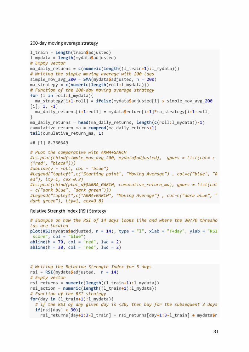
200-day moving average strategy

l_train = length(train$adjusted) l_mydata = length(mydata$adjusted) # Empty vector ma_daily_returns = c(numeric(length((l_train+1):l_mydata))) # Writing the simple moving average with 200 lags simple_mov_avg_200 = SMA(mydata$adjusted, n = 200) ma_strategy = c(numeric(length(roll:l_mydata))) # Function of the 200-day moving average strategy for (i in roll:l_mydata){ ma_strategy[i+1-roll] = ifelse(mydata$adjusted[i] > simple_mov_avg_200[i], 1, -1) ma_daily_returns[i+1-roll] = mydata$return[i+1]*ma_strategy[i+1-roll] } ma_daily_returns = head(ma_daily_returns, length(c(roll:l_mydata))-1) cumulative_return_ma = cumprod(ma_daily_returns+1) tail(cumulative_return_ma, 1)

## [1] 0.760349

# Plot the comparative with ARMA+GARCH #ts.plot(cbind(simple_mov_avg_200, mydata$adjusted), gpars = list(col= c("red", "black"))) #abline(v = roll, col = "blue") #legend("topleft",c("Starting point", "Moving Average") , col=c("blue", "Red"), lty=1, cex=0.8) #ts.plot(cbind(plot_df$ARMA_GARCH, cumulative_return_ma), gpars = list(col= c("dark blue", "dark green"))) #legend("topleft",c("ARMA+GARCH", "Moving Average") , col=c("dark blue", "dark green"), lty=1, cex=0.8)

Relative Strength Index (RSI) Strategy

# Example on how the RSI of 14 days looks like and where the 30/70 thresholds are located plot(RSI(mydata$adjusted, n = 14), type = "l", xlab = "T+day", ylab = "RSI score", col = "blue") abline(h = 70, col = "red", lwd = 2) abline(h = 30, col = "red", lwd = 2)

# Writing the Relative Strength Index for 5 days rsi = RSI(mydata$adjusted, n = 14) # Empty vector rsi_returns = numeric(length((l_train+1):l_mydata)) rsi_action = numeric(length((l_train+1):l_mydata)) # Function of the RSI strategy for(day in (l_train+1):l_mydata){ # if the RSI of any given day is <20, then buy for the subsequent 3 days if(rsi[day] < 30){ rsi_returns[day+1:3-l_train] = rsi_returns[day+1:3-l_train] + mydata$r

32

eturn[day+1:3] rsi_action[day+1:3-l_train] = rep(1,3)} # if the RSI of any given day is >80, then sell for the subsequent 3 days if(rsi[day] > 70){ rsi_returns[day+1:3-l_train] = rsi_returns[day+1:3-l_train] - mydata$return[day+1:3] rsi_action[day+1:3-l_train] = rep(-1,3)}} tail(cumprod(rsi_returns+1), 1)

## [1] 0.908949

# Plot the comparative with ARMA+GARCH #ts.plot(cbind(plot_df$ARMA_GARCH, cumprod(rsi_returns+1)[1:n]), gpars = list(col= c("dark blue", "mediumvioletred"))) #legend("topleft",c("ARMA+GARCH", "RSI") , col=c("dark blue", "mediumvioletred"), lty=1, cex=.65)

Join all Strategies

# Plot of all the strategies in the same graph joint = cbind(plot_df$ARMA_GARCH, plot_df$BUY_HOLD, cum_random, cumulative_return_ma[1:n], cumprod(rsi_returns+1)[1:n]) ts.plot(joint, gpars = list(col= c("dark blue", "red", "orange", "dark green", "mediumvioletred"))) legend("topleft",c("ARMA+GARCH", "Buy and hold", "Random Strategy", "Moving average", "RSI") , col=c("dark blue", "red", "orange", "dark green", "mediumvioletred"), lty=1, cex=.65)

============================================

Performance analytics

joint_returns = as.data.frame(cbind(forecast_df$gain_loss, forecast_df$return, rs_daily_result, ma_daily_returns, rsi_returns[1:length(rs_daily_result)])) joint_returns = as.xts(x = joint_returns, order.by = as.Date(test$date)) colnames(joint_returns) = c("ARMA+GARCH", "Buy and hold", "Random strategy", "Moving average", "RSI") charts.PerformanceSummary(joint_returns[,c(1,2,3,4,5)], colorset = tim8equal, lwd=2, ylim = c(0.4, 1.8),ylog=TRUE)

Relative performance

chart.RelativePerformance(joint_returns[, c(1,3,4,5)], joint_returns[,2], ylim = c(0.3, 5.5), ylog = TRUE, cex.legend = 0.8, colorset = tim8equal, legend.loc = "topleft")