Comparative Effectiveness Based on Observational Data: An ... 2012 Faries.pdf · Simulated...
78
Comparative Effectiveness Based on Observational Data: An Overview Doug Faries BASS 2012
Transcript of Comparative Effectiveness Based on Observational Data: An ... 2012 Faries.pdf · Simulated...

Comparative Effectiveness Based on Observational Data: An
Overview
Doug Faries
BASS 2012

OutlineI. Introduction
II. Standard Comparative EffectivenessAnalyses Based on Propensity Scoring
III. Improvements in Bias Adjustment
IV. Improvements in Sensitivity Analyses (unmeasured confounding)

Part I. Introduction• Need for Observational Research
• Problems with Bias
• Guidances
• Motivating Example

4
Design Continuum
CAN IT WORK? DOES IT WORK?
Randomized Controlled
(Explanatory)
Observational (non-
interventional)
Internal validity
External validity
Randomized

Growing Use of Observational Data
Data Sources◦ Prospective: Trials / Registries / Surveys◦ Retrospective: Insurance Claims, EMRs
Practicalities◦ Large N, Low Cost, Immediate availability,
impracticality of RCTs
Usual Care Data are of Interest:◦ Better data for: Adherence/Persistence, cost,
resource utilization, concom. meds, switching, PROs, treatment patterns, epidemiology, characteristics of populations ….◦ Generalizability

The Observational Research Problem
•Physicians/patients did not select treatment ‘at random’ but based on a variety of factors – so Groups A and B differ in some aspects other than treatment
•A variable is a Confounder if it is associated with both treatment selection and outcome
Selection Bias
Confounders
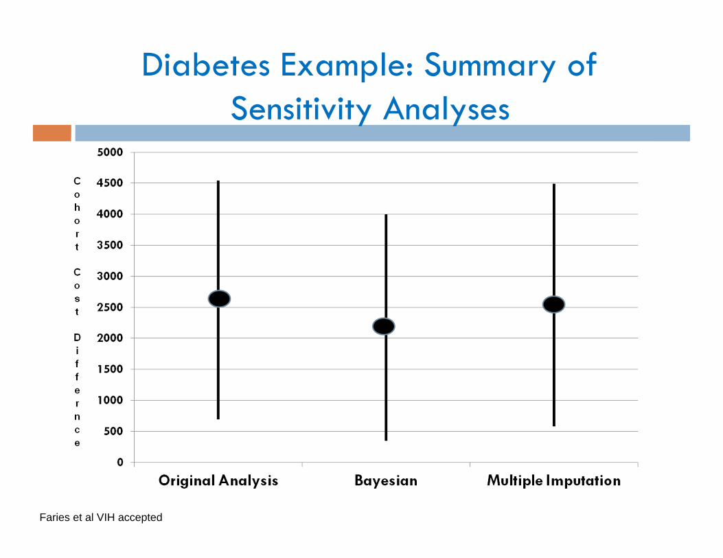
The Observational Research Challenge
Selection Bias
•Physicians/patients did not select treatment ‘at random’ but based on a variety of factors – so Groups A and B differ in some aspects other than treatment
•A variable is a Confounder if it is associated with both treatment selection and outcome
Measured: Information is collected within the studyand statistical adjustment is possible
Unmeasured: Information on the confounder is notavailable from the study
Selection Bias
Confounders

RCTs vs Observational Studies
◦ With randomization – standard methods produce estimation of causal treatment effects
◦ Without randomization (observational) – due to selection bias - standard methods produce only ‘associations’ and not ‘causal effects’ ……… unless selection bias is appropriately controlled
Lower Hiearchy of Evidence for Observational Research

Basic Assumptions for Causal Inference
Propensity Score (or other) adjustments can provide for estimates of the causal group differences under the following assumptions:
No Unmeasured Counfounders ◦ All variables related to both outcome and treatment
assignment are included
Positivity 0 < P(Z=1|X) < 1 for all X
{“sufficient overlap” or “no perfect confounding”}
Correct Statistical Models

Lack of Replication◦ 80% Fail to Replicate or produce substantial less effect
(Ionnidis 2005)◦ “Any claim coming from an observational study is most likely to
be wrong.” – Observational effects were re-examined in RCTs (-5 for 12)
Examples: ◦ Matthews (2008) – “you are what your mother eats”◦ Szydo (2010) – Zodiac sign and Transplants
Clash of Paradigms: Data mining with no multiplicity adjustment (Young 2009)
Controversies with use of Observational Data for Comparative Effectiveness

Controversies … (ctd) Biased Analyses
Low on Hierarchy of Evidence
Lack of Clear Standards
Literature Survey (Pocock 2004) --inadequacies in the analysis and reporting of epidemiological publications
Biggest Problem: Don’t know operating characteristics of such studies so how do we interpret and make decisions on such data?

Recent Guidance Documents PCORI◦ Draft Methodology Report
STROBE◦ Von Elm et al 2007: 22 item checklist
ISPOR Retrospective Research: Good Research Practices (2009)◦ Design and Reporting (Berger et al)◦ Mitigating Bias (Cox et al)◦ Analytic Methods (Johnson et al)
GRACE ◦ Dreyer et al (2010) (Good Research Practices in
Comparative Effectiveness)

DIA Comparative Effectiveness Scientific Working Group
Co-Chairs Matt Rotelli (Lilly) & Alan Menius (GSK)
Goal: Improve the reliability and validity of CER used for making health care decisions.
Subgroup (Lead: Cindy Girman): What Good Looks Like-- Emphasize Core Statistical Principles Under-represented in Current Guidance
A non-competitive collaboration among staff from regulatory agencies, pharmaceutical and biotech companies, and academia to share ideas and advance the science of CER.

Quality Implementation – Rubin’s Key Points (2007)
“Approximate RCTs”◦ Pre-specify the analysis plan / control multiplicity …
Design with No outcome data in sight!◦ Key idea: conduct the design before ever seeing any outcome data; do it in such that future model-based adjustments will give similar point estimates E.g. Propensity Stratification established with baseline data, then various regression models within strata on well balanced patients will give similar results
? What about Retrospective Observational Analyses?

15
Methods Matter! BPRS Changes
Faries et al. 2007

Part II – Standard Methods • Propensity Scoring Approaches
• Implementation Steps• Defining Propensity Model• Confirming Balance• Analysis of cohort differences• Sensitivity Analyses
• Quality Implementation

1. Simulated Observational Depression Study ◦ Faries 2010: Analysis of Observational Health
Care Data Using SAS◦ 5 covariates, N=100 per arm, Outcome:
Remission◦ Goal: Compare Remission Rates between cohorts
2. Type 2 Diabetes Claims Database Analysis◦ Pawaskar et al J Med Econ. 2011◦ Goal: Compare 1-year Total Costs for those
initiating various Type II Diabetes Medications◦ Data Source: Insurance Claims Database

Bias Adjustment ToolsRegression ModelsPropensity Scoring• Instrumental Variables• Newer Techniques:
• Entropy Balancing• Exact / Optimal Matching• Prognostic Scoring• Local Control
• Longitudinal Methods (MSMs)

PS – the conditional probability that a patient received treatment 1 given their set of observed baseline covariates X
Usually computed via logistic regression
Idea: compare treatments between patients with similar propensity scores to allow “apples to apples” comparisons (like ‘stratification’)◦ Practical even when there are a large number of
covariates to adjust for unlike direct stratification

RegressionSimple regression model
with
Y = Trt + PS
StratificationForm (5 or 10) groups of patients with similar PS; Compare cohorts within
each PS strata; then average across the strata
MatchingMatch patients with similar PS, then compare Cohorts within these1:1 (or more complex) matched pairs
Inverse WeightingRun weighted analysis,
weighting each patient by the inverse of their PS

No Gold Standard Recommendation◦ Matching plus sensitivity analyses best for bias control (Austin 2006)
Use sensitivity analysis from a method incorporating a larger proportion of the patients
◦ Stratification + Regression (Lunceford 2004, D’Agostino 2007)
PS Stratification is the main approach
Regression is used WITHIN each propensity score strata to account for residual imbalance within each strata (“Doubly Robust” method)

Regression may be biased when there are large baseline differences between cohorts (as there typically are in observational research)
Propensity Scoring
o A more Robust analysis: makes less assumptions
o Has a built in quality check: “regression analysis may not alert investigators to situations where the confounders do not adequately overlap …” (Shah 2005)
o Allows more flexibility in modeling
o Allows modeling to be done in a blinded fashion
Why not just use Regression?

Estimate the PS(choose PS Model)
Assess Quality of the Bias
Adjustment ( Assess Balance)
Estimate the ‘Treatment Effect’ (matching, stratification,
combination)
Sensitivity Analysis
(Assumptions, Generalizability,
Unmeasured Confounding)

Thou shalt examine covariates for collinearity
Thou shalt value parsimony Thou shalt test predictors for
statistical significance Thou shalt have 10 times as many
subjects as predictors Thou shalt carefully examine
regression coefficients
I.
II.
III.
IV.
V.
Acknowledge:Thomas Love

10 Commandments of Choosing a Propensity Model
Thou shalt perform bootstrap analyses to assess shrinkage
Thou shalt perform regression diagnostics and evaluate residuals
Thou shalt hold out a sample for model validation
Thou shalt employ external validation on a new sample of data
VI.
VII.
VIII.
IX.

10 Commandments of Choosing a Propensity Model
10th Commandment:
Instead – simply ensure that the model adequately balances the covariates
“the success of the propensity score modeling is judged by whether balance on pretreatment characteristics is achieved between the treatment and control groups …” (D’Agostino 2007)
Ignore the previous 9

Depression Example: Distribution of Propensity Scores

SSRI
Example What if Little Overlap?

Draft: Work in Progress. Internal Use only
SSRI
Example What if Little Overlap?
No Causal Inference on Full Population without Additional Strong Assumptions
- Stop- Revise PS model (unlikely)?- Proceed but only in small subset- Trade bias for generalizability
(caution!)

Matching Decisions1. Distance Measure
• Absolute Diff in PS; Mahalanobis; ….
• Caliper used to limit poor matches
• Rosenbaum (2010) Rank Based Mahalanobis with 0.2 SD of PS as caliper
2. Ratio• 1:1 (best balance); 1:n; 1:variable; var:1 & 1:var
3. Algorithm• Greedy or Optimal / Full or Matching with
Replacement or ….

Methods: Nearest Neighbour (Greedy)
• Most frequently used matching algorithm
• 1st Treated patient is matched to closest Control patient (this match is then fixed), 2nd Treated patient is matched …..
• Does not optimize any overall measure of balance
• Different match each time you sort the data set

Trt A:
Trt B:
5.7 4.0 3.4 3.1
5.5 5.3 4.9 4.9 3.9
Greedy Algorithm Example

Trt A:
Trt B:
5.7 4.0 3.4 3.1
5.5 5.3 4.9 4.9 3.9
Greedy Algorithm Example-- With a Caliper of 1.0
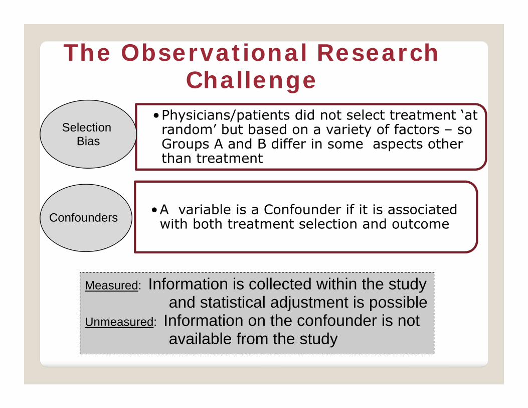
(Full) Optimal MatchingOptimal Matching
- Minimize sum of absolute differences in distance measure- Does not depend on order of the dataset
5.7Trt A:
Trt B:
4.0
3.4
3.1
5.5
5.3
4.9
4.9
3.9
Avg imbalance 0.85
Optimal Full Matching (Hansen 2004)- Also allows 1:many and many:1 matches
5.7Trt A:
Trt B:
4.0
3.4
3.1
5.5
5.3
4.9
4.9
3.9
Avg imbalance 0.51

Depression Example: Matching Analyses
Used (1:1) PS Matching as the primary analysis – Greedy Algorithm
Matched 74 pairs (of 96 possible)
Need to summarize generalizability
Next Assess the Balance• D’Agostino: quality of the PS adjustment is judged
by the balance acheived

Assessing the Balance
• Hypothesis Testing• Common – but sample size dependent
• Standardized Differences• Recommended (Austin, Imbens)• “difference in means / pooled SD” (not sample
size dependent)• Rule of Thumb: < 0.1 is OK

Trt AN=96
Trt BN=96 P-val
Trt AN=74
Trt BN=74 P-val
Age 42.8 47.2 .031 44.0 43.7 .889
Male 17.7 21.9 .469 18.8 20.3 .824
PHQ 13.7 16.0 .004 14.9 14.7 .880
Married 62.5 66.7 .546 67.2 64.1 .710
Work 59.4 31.3 <.01 46.9 43.8 .723
…
Pre-Matching Post-Matching

Balance: Standardized Differences
Work
Age
PHQ1
Spouse
Gender
Standardized Difference

Compute PS
Group PS into homogeneous Strata◦ How Many? Grouping on Quintiles 5 most common (Cochran
1968), 10 if larger N ….. Imbens (2010): Data Driven algorithm – split if not
sufficiently homogeneous
Assess Balance (within strata)
Trim non-overlapping PS if necessary

Analysis◦ Compare Treatments Within Strata, then Average
Across Strata Difference in Means Within Strata Regression Within Each Strata to account for residual
imbalance Stratified bootstrapping if non-normal outcomes

Depression Example: Propensity Score Strata

Balance Produced by Propensity Scores: Variable: Work
Overall

Propensity Score Bins
Strata 1: Compare Cohorts using Regression (to adjust for residual confounding) in Stratum 1. Then repeat for Strata 2-5, then average across the Strata

Part III – Improvements in Bias Adjustment
What is New?
Entropy Balancing Example

NEW AND IMPROVED BIAS ADJUSTMENT?
Exact Matching (plus) Prognostic Scores Optimal Matching Entropy Balancing Local Control ……

ENTROPY BALANCING(HAINMUELLER 2012)
Finds the ‘weights’ for each patient that …. Produces balanced means and variances Between any number of cohortsKeeps weights as close to ‘1’ as possible while
achieving balance
Compare Cohorts using Weighted analysis
Maximum entropy reweighting scheme that calibrates unit weights so that the reweighted treatment and control group satisfy a potentially large set of pre-specified balance conditions

ENTROPY BALANCINGAdvantages
-No need for iterative assessment of balance-Handles > 2 Treatments-Can balance on more than just the mean (any specified moments or interactions …..)-Does not require access to outcome data-Can specify target population of interest
Limitations
Unable to find solution / Large Weights

EXAMPLE: ENTROPY BALANCING
Depression Data Balance means and variances …. on 5 covariates …. between 3 treatment groups Target Population: Full Population (ATE)
Code: http://www.mit.edu/~jhainm/Paper/ebalance.pdf

Balance: Original Analysis
Trt AN=96
Trt BN=96 P-val
Trt AN=74
Trt BN=74 P-val
Age 42.8 47.2 .031 44.0 43.7 .889
Male 17.7 21.9 .469 18.8 20.3 .824
PHQ 13.7 16.0 .004 14.9 14.7 .880
Married 62.5 66.7 .546 67.2 64.1 .710
Work 59.4 31.3 <.001 46.9 43.8 .723
…
Pre-Matching Post-Matching

Balance: Produced by Entropy
Trt AN=96
Trt BN=96
Trt C N=94
P-val
Age 45.3 45.3 45.3 1.00
Male 24.5 24.5 24.5 1.00
PHQ 14.8 14.8 14.8 1.00
Married 59.8 59.8 59.8 1.00
Work 44.1 44.1 44.1 1.00
…
Balanced on Means and Variances; Balanced across all 3 groups; Better balance

SUMMARY OF ENTROPY WEIGHTS
Ntx Obs N Mean Std Dev Min Max
___________________________________________________________
0 96 96 1.00 0.65 0.08 3.70
1 96 96 1.00 0.54 0.28 2.94
2 94 94 1.00 1.36 0.08 10.02
____________________________________________________________

DEPRESSION RESULTS: ALL METHODS
Trt A Trt B P-val
Original Data 62.5% 46.9% .030
Propensity Match 60.9% 53.1% .372
Propensity Strata 58.6% 50.1% .218
Entropy 54.8% 50.4% .524

Part IV – Sensitivity • Focus Here: Unmeasured Confounding
• Full Sensitivity should include• Assessment of Generalizability, Models, Statistical Assumptions, Missing Data ….
• Unmeasured Confounding Methods• Rule Out• External Adjustment• Internal Adjustment
• Propensity Calibration / Bayesian Modeling / Multiple Imputation / Inverse Weighting
• Prior Event Rate Adjustment

Example: Type 2 Diabetes Comparison(Pawaskar J Med Econ 2011)
Utilized Propensity Score Matching to compare costs between patients initiating Byetta vs Insulin Glargine
Insurance Claims Database Analysis◦ N1 = 7255, N2 = 2819 ◦ Adjusted for patient demographics, comorbidities,
complications, resource use and costs of care in 6 month pre-initation period.
◦ Unable to adjust for: BMI, duration of diabetes, glycemic control

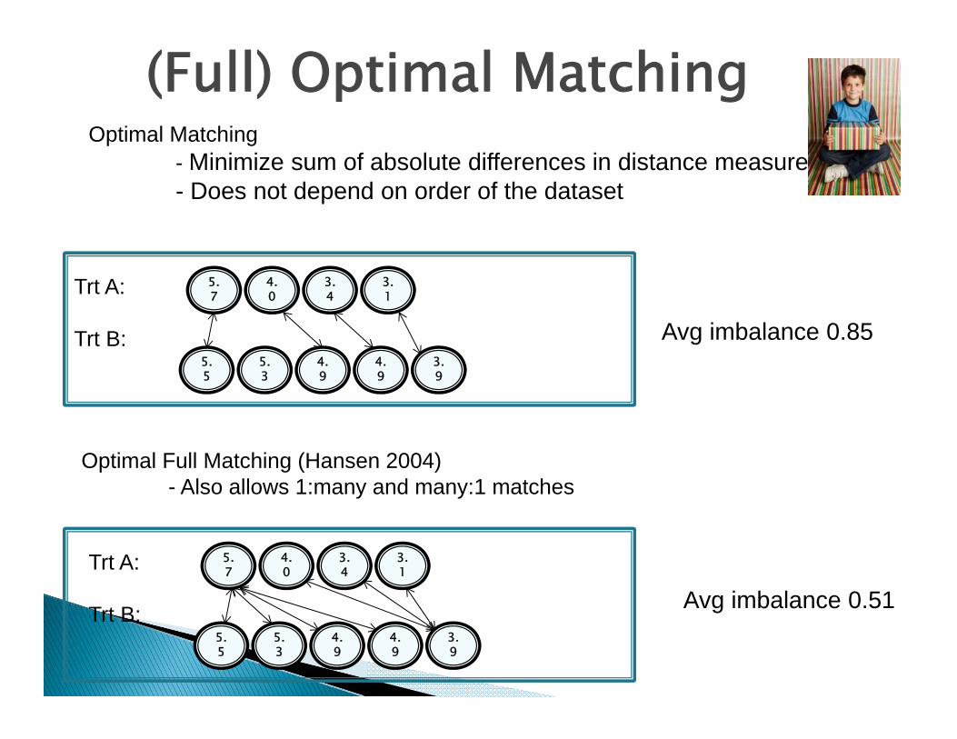
Diabetes Example: Original Results
Estimated mean cost difference
$2597 (690, 4542) p < .05

Interpretation Depends on Assumption of No Unmeasured Confounding
What should I do about unmeasured confounding?

Current State of the Union Regarding Unmeasured Confounding
What should I do about unmeasured confounding?
Just mention it as a limitation in the
Discussion Section and move on!

EXPERT
There are new methods in the literature! “Best Practices” include sensitivity analyses

Unmeasured Confounding Options
Internal
UnmeasuredConfounding
External
1) Bayesian2) Multiple Imputation3) Inverse Weighting4) Propensity Calibration
NoneInformationAvailable
Method 1) Rule Out2) IV
1) Bayesian2) Algebraic

Concept: Quantify how strong and imbalanced a confounder would need to be in order to explain (“rule out”) the observed result.
Rule-out Method (no data)
This approach attempts to find all combinations of1) the confounder‐outcome relationship and 2) the confounder‐treatment relationship,‐
necessary to move the observed point estimate to zero.

File name/location Company ConfidentialCopyright © 2000 Eli Lilly and
C
Rule-out Method – Diabetes Example
Con
foun
der –
Coh
ort
Ass
ocia
tion
Confounder - Outcome Association
So, a confounder occurring in 20% more patients in Cohort A
(compared to Cohort B) which results in $15,000 higher cost per patient
would eliminate the observed difference
Trt A is Not Less Costly
Trt A remains
Less Costly

Diabetes Example
Internal Data Sensitivity Opportunity!! No measure of glycemic control was available in the original
claims database. However, after linking with a laboratory file, A1C values were obtained in a subset (about 25%) of the sample;
Results: Estimated mean cost difference
$2597 (690, 4542) p < .05

Information Available: Internal
With Internal data can avoid transportability assumption and can account for correlation between unmeasured confounder and measured confounders
Concept: Use information from the patients in the study (e.g. subsample of chart review data for a retrospective claims database study) to estimate parameters regarding unmeasured confounding

Information Available: Internal
Methods
Propensity Score CalibrationSturmer et al (Am J Epi 2005)
Bayesian ModelingMcCandless (Stat Med 2007)
Multiple ImputationToh et al (Pharmacoepi Drug Saf 2012)

Bayesian Twin Regression Models
Concept: Bayesian models naturally incorporate additional sources of information – such as
internal subset data or external information from other studies ‐ through prior distributions
MeasConfUnmConfTreatmentOutcome *3*2*10
MeasConfreatment)1UnmConf(Logit TP
Implementation: WinBUGS (SAS 9.3 code upcoming)
Internal data serves in essence as informative prior information for parameters relating to unmeasured confounder

Bayesian Twin Regression Models
MeasConfUnmConfTreatmentOutcome ***10
MeasConf)1UnmConf(logit TRTP
Priors:
Uninformative:
Informative:
,,
210 ,,,
R1

Slide 66
R1 may want to further comment on flexibility here in sense that this is continuous outcome and binary covariate. need not be the case ...ie , can be other combinations in terms of binary outcome/binary confounder, etc, so here we highlight a frameworkRM36604, 3/15/2011

Keys to Bayesian Approach
• Incorporates available info via Informative Priors• Best available data – whether internal or External • Informative Priors – not just adding uncertainty
(McCandless 2007)
• Yields a posterior distribution for the treatment effectadjusted for the unmeasured confounder U.
• Fixed Modeling failed to incorporate variability (Schneeweiss 2006)
• Flexible data driven model• No restrictions on relationships on associations between variables as in PS Calibration (Sturmer 2007).

Missing Data Multiple Imputation (for internal data)
Imputation Model: Treatment, Measured Covariates, and Outcome
Used > 5 replications due to amount of missing data
Implementation: PROC MI in SAS
Concept: This is a missing data problem – use a well accepted method ‐‐Multiple
Imputation!
Diabetes Example: Summary of Sensitivity Analyses
Faries et al VIH accepted

Unmeasured Confounding Conclusions
Comparative effectiveness research should include ‘Unmeasured Confounding’ sensitivity to help consumers of the data understand the robustness of the findings.
Bayesian and MI methods are promising approaches- naturally incorporate additional info (internal or external)- can use internal data to avoid development of prior.
Lots of Remaining Questions
• When is one method preferred to another?• How much ‘internal data’ is needed for each method?• When is it cost effective to obtain the internal information as opposed to more easily
available external data?

Overall Summary
Causal Inference from Observational Data requires making un-testable assumptions◦ We DON’T KNOW the operating characteristics of current
practices◦ Publications are not sufficiently transparent for
appropriate interpretation of the value/quality Quality Analyses includes:◦ Pre-specification, appropriate bias adjustment, replication,
and sensitivity analyses …. CORE STATISTICAL PRINCIPLES Newer Methods are very promising for:◦ Better bias adjustment (for measured confounders)◦ Better Sensitivity Analyses (for unmeasured confounders)

Backup Slides
Draft: Work in Progress. Internal Use only

73
Schizophrenia Pragmatic Trial Example (Tunis 2006)Randomized, Open Label, 1-Year, Cost
Effectiveness Study 3 treatment regimens (total N = 664)
• Olanzapine / Risperidone / Conventionals
Naturalistic: patients may switch, stop, augment, change doses … and remain in study
• Primary Analysis: Cost Effectiveness• Effectiveness Outcome: BPRS Total Score

Propensity Score Calibration
Two propensity scores (PS) are calculated: - “Error Prone” PS: utilizes only covariates available
in the full sample - “Gold Standard” PS: utilizes additional confounding
covariates (in subset with all covariates)
Regression calibration (measurement error modeling) is then applied to adjust the regression coefficients and thus compensate for the unmeasured confounding.
Concept: Utilize additional data - variables not in full sample but available for a subset of patients - to modify the propensity score adjustment

Propensity Score Calibration
Validity relies on surrogacy of the error prone propensity for the gold standard propensity. ◦ “error prone PS” must be independent of the
outcome given “gold standard PS” and treatment.
For our example – surrogacy assumption not clearly satisfied Correlations of A1C & Outcome was negative Correlations of Other Covariates & Outcome was
positive

Propensity Score Calibration (ctd)
Error Prone Propensity Score Model (PSEP)
Gold Standard Propensity Score Model (PSGS)
Calibration Model: EPGS PSXPSE 210][
),,...,,|1Pr( 21 nGS zzzXPS
),...,,|1Pr( 21 nEP zzzXPS

Why not just use Regression?
D’Agostino 2007
•“regression” can produce biased estimates of treatment effects if there is extreme imbalance of the background characteristics and/or the treatment effect is not constant across values of the background characteristics”
Rule of Thumb (Imbens)•If all normalized differences are less than 0.1 the choice of
adjustment method is unimportant, whereas for differences exceeding 0.25 simple adjustment methods such as linear covariance adjustment are unlikely to be adequate