Comparative Analysis of Exchange Rate Fluctuations on Output and Price:

Evidence from Middle Eastern Countries

Magda Kandil* Senior Economist, IMF Institute

International Monetary Fund 700 19th Street, N.W.

Washington, D.C. 20431 Email: mkandil@imf.org

and Ida Aghdas Mirzaie Assistant Professor

Department of Economics and Finance John Carrol University 20700 North Park Blvd.

University Heights, Ohio 44118 Email: imirzaie@icu.edu

* The views presented are those of the author and do not necessarily reflect the views of the IMF or IMF Policy

. Contents Page

I. Introduction ............................................................................................................................3

II. Theoretical Background ........................................................................................................5 A. Aggregate Demand ...................................................................................................6 B. Aggregate Supply......................................................................................................8 C. Market Equilibrium...................................................................................................9

III. Empirical Models...............................................................................................................10

IV. Empirical Results...............................................................................................................15 A. Fluctuations in the Face of Policy Shifts ................................................................15 B. Fluctuations in the Face of Aggregate Demand Shifts............................................16

V. Summary and Conclusion ...................................................................................................17

References................................................................................................................................37 Text Tables 1 Nonlinear 3SLS Parameter Estimates, using money supply and government spending ......20 2 Nonlinear 3SLS Parameter Estimates, using nominal GDP .................................................23 A1 The KPSS Statistics for Null of Level Stationary..............................................................28 A2 Cointegration Test Results .................................................................................................29 A3 Cointegration Test Results .................................................................................................30 A4 The Results of Endogeneity Tests......................................................................................31 Appendices Econometric Methodology.......................................................................................................35 Data Sources ............................................................................................................................36

- 3 -

I. INTRODUCTION

There has been an ongoing debate on the appropriate exchange rate policy in developing countries. The debate focuses on the degree of fluctuations in the exchange rate in the face of internal and external shocks. Exchange rate fluctuations are likely, in turn, to determine economic performance. In judging the desirability of exchange rate fluctuations, it becomes, therefore, necessary to evaluate their effects on output growth and price inflation. Demand and supply channels determine these effects. A depreciation (or devaluation) of the domestic currency may stimulate economic activity through the initial increase in the price of foreign goods relative to home goods. By increasing the international competitiveness of domestic industries, exchange rate depreciation diverts spending from foreign goods to domestic goods. As illustrated in Guittian (1976) and Dornbusch (1988), the success of currency depreciation in promoting trade balance largely depends on switching demand in proper direction and amount, as well as on the capacity of the home economy to meet the additional demand by supplying more goods1. While the traditional view indicates that currency depreciation is expansionary, some theoretical views have suggested some contractionary effects. Meade (1951) discusses this theoretical possibility. If the Marshall-Lerner condition is not satisfied, currency depreciation could produce contraction.2 Hirschman (1949) points out that currency depreciation from an initial trade deficit reduces real national income and may lead to a fall in aggregate demand. Currency depreciation gives with one hand, by lowering export prices, while taking away with the other hand, by raising import prices. If trade is in balance and terms of trade are not changed these price changes offset each other. But if imports exceed exports, the net result is a reduction in real income within the country. Cooper (1971) confirms this point in a general equilibrium model. Diaz-Alejandro (1963) introduced another argument for contraction following devaluation. Depreciation may raise the windfall profits in export and import-competing industries. If money wages lag the price increase and if the marginal propensity to save from profits is higher than from wages, national savings will go up and real output will decrease. Krugman and Taylor (1978) and Barbone and Rivera-Batiz (1987) have formalized the same views. Supply-side channels further complicate the effects of currency depreciation on economic performance. Bruno (1979) and Wijnbergen (1989) postulate that in a typical semi-industrialized country where inputs for manufacturing are largely imported and cannot be 1 Empirical support of this proposition for Group 7 countries over the 1960-89 period is provided in Mendoza (1992). 2 The Marshall-Lerner condition states that devaluation will improve the trade balance if the devaluing nation's demand elasticity for imports plus the foreign demand elasticity for the nation's exports exceed 1.

- 4 -

easily produced domestically, firms' input cost will increase following a devaluation. As a result, the negative impact from the higher cost of imported inputs may dominate the production stimulus from lower relative prices for domestically traded goods. Gylfson and Schmid (1983) provide evidence that the final effect depends on the magnitude by which demand and supply curves shift because of devaluation.3 To summarize, currency depreciation increases net exports and increases the cost of production. Similarly, currency appreciation decreases net exports and the cost of production. The combined effects of demand and supply channels determine the net results of exchange rate fluctuations on real output and price.4 This paper revisits the relationship between exchange rate fluctuations and economic activity in developing countries. The contribution of the theory is in treating the process of forming rational forecasts of the exchange rate. Recent experiences of currency crises have brought to the forefront the importance of anchoring agents’ forecasts in the design of an appropriate exchange rate policy. Hence, the theory aims to separate the effects of anticipated shifts in the exchange rate from unanticipated deviations and agents’ forecasts. The theoretical investigation introduces a model that decomposes movements in the exchange rate into anticipated and unanticipated components using rational expectations. Anticipated movement in the exchange rate is assumed to vary with agents' observations of macro-economic fundamentals, which determine changes in the exchange rate over time. Deviation in the realized exchange rate from its anticipated value captures the unanticipated component of the exchange rate. In this context, the output supplied varies with unanticipated price movements and the cost of the output produced. Anticipated exchange rate movements determine the cost of the output produced. In contrast, unanticipated exchange rate movements determine economic conditions in three directions: net exports, money demand, and the output supplied. The solution of the model demonstrates the effects of demand and supply channels on the output and price responses to unanticipated changes in the exchange rate. Based on theory's solutions, empirical models are formulated for output and price. The models incorporate demand and supply shifts as well as exchange rate shifts. Exchange rate fluctuations are assumed to be randomly distributed around a steady-state stochastic trend

3 Hanson (1983) provides theoretical evidence that the effect of currency depreciation on output depends on the assumptions regarding the labor market. Solimano (1986) studies the effect of devaluation by focusing on the structure of the trade sector. Agenor (1991) introduces a theoretical model for a small open economy and distinguishes between anticipated and unanticipated movement in the exchange rate. Examples of empirical investigations include Edwards (1986), Gylfason and Radetzki (1991), Roger and Wang (1995), Hoffmaister and Vegh (1996), Bahmani (1998), Kamin and Rogers (2000), and Kandil and Mirzaie (2002, and 2003). 4 For an analytical overview, see Lizondo and Montiel (1989).

- 5 -

over time. This trend varies over time with agents' observations of macro-economic fundamentals. Positive shocks to the exchange rate indicate an unanticipated increase in the Foreign currency price of domestic currency, i.e., unanticipated currency appreciation. Similarly, negative shocks indicate unanticipated depreciation of the exchange rate. The data under investigation are for a sample of 11 developing countries in the Middle East. The real exchange rate is constructed by multiplying the value of each country's currency in terms of the U.S. dollar by the relative price between the two countries. Hence, the real exchange rate accounts for the relative prices in the domestic economy relative to foreign price in the largest economy of the world. The relative price channel is important to the analysis of exchange rate fluctuations given the high inflationary experience in developing countries. Accordingly, the empirical investigation will combine the nominal exchange rate policy with movements in domestic price inflation relative to that of a major international price to determine the implications of fluctuations in the real exchange rate on economic performance in developing countries. The results clearly illustrate the different effects of anticipated and unanticipated shifts of the exchange rate on the macroeconomy. Anticipated shifts have limited effects, which minimize the role of rational forecast in guiding production plans in many developing countries. In contrast, unanticipated deviation of the realized exchange rate from agents’ forecasts induce random fluctuations, with varying effects, positive or negative, on output growth and price inflation. Such fluctuations signal the importance of varying the exchange rate in line with agents’ forecasts, striking an appropriate balance between necessary flexibility to ensure competitiveness while maintaining agents’ confidence to hold domestic currency. The remainder of the paper is organized as follows. Section II presents the theoretical model. Section III outlines the empirical models. Section IV presents empirical results. The summary and conclusion are presented in section V.

II. THEORETICAL BACKGROUND

In the real world, stochastic uncertainty may arise on the demand or supply sides of the economy. Economic agents are assumed to be rational. Accordingly, rational expectations of demand and supply shifts enter the theoretical model. Economic fluctuations are then determined by unexpected demand and supply shocks impinging on the economic system. The paper introduces a macro-economic model that incorporates exchange rate fluctuations of the domestic currency. Fluctuations are assumed to be realized around a steady-state trend that is consistent with variation in macro-economic fundamentals over time. Uncertainty enters the model in the form of disturbances to both aggregate demand and aggregate supply. Within this framework, aggregate demand is affected by currency depreciation through exports, imports, and the demand for domestic currency, and aggregate supply is affected through the cost of imported intermediate goods. The model demonstrates theoretically that unanticipated currency depreciation decreases real output

- 6 -

growth, via the effect on the supply side. However, the relationship between unanticipated currency depreciation and aggregate demand makes the final outcome inconclusive.

A. Aggregate Demand

The demand side of the economy is specified using standard IS-LM equations with a modification for an open economy. The specifications below describe equilibrium conditions in the Goods and Money markets. All coefficients are positive and throughout the paper, lower case denotes the logarithm of the corresponding level variable. The subscript t denotes the current value of the variable.

1 ,t o dtc c c y= + 10 1c< < (1)

dt t ty y t= − (2)

0 1 ,t tt t t y= + 1 0t > (3)

0 1 ,t ti i i r= − 1 0i > (4)

*t t

tt

S PREP

= (5)

( )0 1 log ,t tx x x RE= − 1 0x > (6)

( )0 1 2 log ,t t tim m m y m RE= + + 1 2, 0m m > (7)

t t t t t ty c i g x im= + + + − (8)

[ ] ( )1 1( ) ,t t t t t t t t t tm p r E p p y E s sλ φ θ+ +− = − + − + + − , , 0λ φ θ > (9)

Equations (1) through (8) describe equilibrium conditions in the Goods market. In equation (1), real consumption expenditure, c, varies positively with real disposable income, yd. In equation (2), disposable income is defined to be the net of real income, y, minus taxes, t. In equation (3), real taxes are specified as a linear function of real income. In equation (4), real investment expenditure, i, varies negatively with the real interest rate, r. In equation (5), let the domestic price level be represented by P and the foreign price level in foreign currency by P*. S denotes the spot price of domestic currency. It measures the number of foreign currency units per units of domestic currency. RE is the price of domestically produced goods and services relative to the prices of foreign produced goods and services, i.e., the real exchange rate of the domestic currency. When RE increases, the domestic currency appreciates in real terms. The value of RE measures the degree of competitiveness of foreign produced goods and services relative to those

- 7 -

produced domestically.5 In equation (6), real exports are related to an autonomous element, x0, which rises when the income level abroad rises, and to relative prices. The inverse relationship between RE and x, in (6), refers to the fact that when the domestic price is higher relative to foreign goods, exports will decrease. In equation (7), real imports, im, are assumed to rise with the level of real income and the real exchange rate of the domestic currency. Equation (8) describes the equilibrium condition in the goods market. Real government spending, g, is assumed to be exogenous. The total expenditure by domestic residents in real terms (y) is the sum of real consumption expenditure (c), real investment (i), real government spending (g), and net exports (the real value of exports, x, minus the real value of imports, im). Substituting all equations into the equilibrium condition for the goods market results in the expression for real income. It is a function of the exchange rate, the domestic price level, the foreign price level, and the domestic interest rate. This expression is the IS equation which describes the negative relationship between real income and the real interest rate. In equation (9), equilibrium in the money market is obtained by equating the demand and supply of real money balances. The real money supply is determined by nominal balances, m, deflated by price, p. The demand for real money balances is positively related to real income and inversely related to the nominal interest rate. The nominal interest rate is defined as the sum of the real interest rate and inflation expectation at time t. Etst+1 is the expected future value of the foreign currency at time t. It is assumed that citizens in each country must hold domestic money for transactions purposes but they may speculate by holding foreign money.6 An unexpected temporary appreciation of the domestic currency in period t would lead to speculation of depreciation in period t+1 to restore the steady-state normal trend of the exchange rate, i.e., (Etst+1-st)<0.7 Consequently, agents decrease the speculative demand for domestic currency, establishing a positive relationship between the demand for real money balances and agents' expectation of the exchange rate relative to the current value of the currency. The LM equation is determined by the equilibrium condition in the money market. It establishes a positive relationship between real income and the real interest rate. Solving for the interest rate, r, from the LM equation and substituting the result into the IS equation results in the equation for aggregate demand.

5 For a similar definition, see (Shone 1989). 6 For a similar discussion, see(Buiter 1990). 7 Agents are encouraged to dispose of domestic currency following unexpected appreciation. Alternatively, speculative attacks may start if agents perceive the exchange rate to be overvalued (e.g., in the event of a peg that cannot be sustained). Hence, the demand for domestic currency decreases.

- 8 -

B. Aggregate Supply

On the supply side, output is produced using a production function that combines labor, capital, energy and imported intermediate goods. When the currency depreciates (or is devalued), it is more expensive to buy intermediate goods from abroad. The price of energy is paid in dollars in order to isolate this variable from fluctuations in the exchange rate. To illustrate, the level of gross domestic output, Q, is produced using a production function that combines imported intermediate goods, U, labor, L, and the capital stock, K. The production function is Cobb-Douglas in U and L, assuming fixed capital stock.8 In addition, the production function is dependent on the energy price, Z. Accordingly, the supply-side of this economy can be summarized in equations (10) through (14) as follows:

1 tZt t tQ L U eδ δ −−= (10)

t t t tY Q RE U= − (11)

{ } 1log , 01

dt t t t tl u w p zη δ η

δ= − − + − = >

− (12)

( ) ( ){ }1 log 1 logt t t tu l z REδδ

= + − − + (13)

{ }1log , 0s

t t t tl w E pη δ ω ω−= + − > (14)

Equation (10) specifies the level of gross domestic output produced, assuming complementary relation between the labor input and imported intermediate goods. Equation (11) defines domestic value added (output supplied) or the difference between gross domestic output and the amount of real intermediate imports.9 To derive the demand for inputs, the marginal product of L and U is calculated and the results are equated with the real cost of labor (the real wage) and the real price in domestic currency of imported intermediate goods (the real exchange rate). Taking log transformation of the first-order conditions and rearranging produces equations (12) and

8 Fixing the capital stock excludes the possibility that depreciation may increase labor productivity by stimulating capital accumulation. 9 This definition follows Agenor (1991) where he introduces a model and assumes intermediate goods are necessary for the production process and cannot be produced domestically.

- 9 -

(13). The demand for labor varies negatively with the real wage and positively with imported intermediate goods. Similarly, the demand for imported intermediate goods increases with the labor input. The appreciation of currency decreases the real price of imported intermediate goods and, hence, increases the demand for these goods. Furthermore, a rise in the energy price decreases the demand for labor and imported intermediate goods. Equation (14) hypothesizes a positive log-linear relationship between labor supply and expected real wage. The supply of labor increases with an increase in the nominal wage relative to workers' expected price at time t-1. The nominal wage solution is obtained by equating labor demand and labor supply. Substituting the nominal wage into labor demand results in the solutions for employment and imported intermediate goods. Substituting for l and u into the log transformation of equation (10), results in an equation for gross domestic output supplied. Substituting the result into the log transformation of equation (11) results in an equation for the aggregate supply of domestic value added. For details of the model solution, see Kandil and Mirzaie (2003). Aggregate supply has a direct positive relationship with output price surprises. Workers decide on labor supply based on their expectation of the aggregate price level. An increase in aggregate price relative to workers' expectations increases the demand for labor and, hence, the nominal wage. A rise in expected real wage increases employment and, hence, the output supplied. In addition, the aggregate supply moves positively with the foreign currency price of domestic currency. Currency appreciation decreases the cost of imported goods and increases the output supplied. Further, the output supplied varies negatively with changes in the energy price. 10

C. Market Equilibrium

Internal balance requires that aggregate demand for domestic output be equal to aggregate supply of domestic output at full employment. It is assumed that demand and supply shifts in the model are constructed of two components: anticipated (steady-state) component and an unanticipated (random) component. The combination of demand and supply channels indicates that real output depends on unanticipated movements in the exchange rate, the money supply, government spending, and the energy price.11 In addition, supply-side channels establish that output varies with anticipated changes in the exchange rate and the energy price. 10 This assumption assumes the country is an energy importer. Of course, in an oil producing country an increase in the energy price is likely to have a positive effect on the output supplied. 11 With the exception of the energy price, shocks are assumed to fluctuate in response to domestic economic conditions or in response to external vulnerability, e.g., capital mobility or fluctuations in foreign reserves.

- 10 -

Given demand-side channels, aggregate demand increases with an unexpected increase in government spending or the money supply, creating positive price surplusess and, hence, increasing output and price in the short-run. The allocation of price surpluses between output growth and price inflation is dependent on the slope of the short-run supply curve, as determined by elasticities underlying the supply side of the economy. Changes in the energy price, both anticipated and unanticipated, increase the cost of the output produced, decreasing output and raising prices.12 The complexity of demand and supply channels may determine the results of exchange rate fluctuations as follows: 1. In the goods market, a positive shock to the exchange rate of the domestic currency (an unexpected appreciation) will make exports more expensive and imports less expensive. As a result, the competition from foreign markets will decrease the demand for domestic products, decreasing domestic output and price.

2. In the money market, a positive shock to the domestic currency (an unexpected temporary appreciation) relative to anticipated value, prompts agents to hold less domestic currency and decreases the interest rate. This channel moderates the contraction of aggregate demand and, therefore, the reduction in output and price in the face of a positive exchange rate shock.

3. On the supply side, a positive shock to the exchange rate (an unanticipated appreciation) decreases the cost of imported intermediate goods, increasing domestic output and decreasing the cost of production and, hence, the aggregate price level.13

III. EMPIRICAL MODELS

The empirical investigation analyzes annual time-series data of real output and price in 11 developing countries in the Middle East. The sample period for investigation is 1971-

12 The price level may rise unexpectedly in response to energy price shocks, creating incentives to increase the output produced. This channel moderates the reduction in output and the rise in price in response to energy price shocks. For a detailed theoretical illustration, see Kandil and Woods (1997). The moderating effect of the rise in price is further reinforced in the theoretical model through the increase in the real exchange rate, reducing the real cost of intermediate imported goods. 13 Other supply-side channels may reinforce the negative effect of currency depreciation on the output supplied. Recent crises in developing countries have illustrated the mismatch effects of currency depreciation on balance sheets. Many developing countries rely on foreign sources of financing. Currency depreciation increases the cost of borrowing by raising the burden of foreign currency denominated liabilities. A higher cost of borrowing has an adverse effect on the supply-side of the economy, further reinforcing the negative effect on out put growth and the positive effect on price inflation in the theoretical model.

- 11 -

2000 (see Appendix B for details). The countries are selected based on the availability of the time series data necessary for investigation. These countries have not been investigated thoroughly for the theoretical implications under consideration. Moreover, the countries are quite diverse on several grounds: domestic policy, per capita GDP the exchange rate regime, and openness. We aim to test the effects of exchange rate fluctuations in a random sample of diverse countries which renders the time-series estimation of individual country data worth while. Over time, it is assumed that real output growth and price inflation fluctuate in response to aggregate domestic demand shocks, energy price shocks and exchange rate shocks. Shocks are randomly distributed over the time span under investigation. Exchange rate shocks are assumed to be distributed around an anticipated stochastic steady-state trend. This trend varies with agents' observations of macroeconomic fundamentals that are likely to determine the exchange rate14. Positive shocks to the price of domestic currency in foreign currency represent unanticipated appreciation around this trend. Negative shocks represent unanticipated currency depreciation. Over the time span under investigation, these shocks are assumed to occur with equal probability around the stochastic moving trend. Detailed econometric methodology is provided in Appendix A. Detailed description and sources of all data are described in Appendix B. The model specification is based on the results of the test for non-stationarity of real output.15

( )( ) ( )

0 1 1 2 1 3 1 4 1

5 1 6 1 7 1 8 1

9

( )t t t t t t t t t t t

t t t t t t t t t t

yt t

Dy A A E Dz A Dz E Dz A E Dm A Dm E Dm

A E Dg A Dg E Dg A E Drs A Drs E Drs

A EC v

− − − −

− − − −

= + + − + + −

+ + − + + −

+ +

(15)

The test results are consistent with non-stationary real output for all countries under investigation. Given these results, the empirical model of real output is specified in first

14 The theoretical model does not determine the exchange rate or other policy variables endogenously. Instead, the model is solved for the reduced forms that determine the responses to exogenous policy shocks. In theory, shocks approximate unanticipated components of policy shifts based on rational expectations. For example, an overvalued exchange rate represents an unanticipated currency appreciation around agents' expectation of what the exchange rate should be. Econometrically, the anticipated component varies with agents' observations of macro-economic fundamentals, as described in Appendix A. Random shocks capture exogenous fluctuations around the moving trend over time. 15 For details, see Kwiatkowski et. al. (1992). Non-stationarity indicates that, real output follows a random-walk process. Upon first-differencing, the resulting series is stationary, which is the domain of demand and supply shifts, as specified in theory.

- 12 -

difference form where D(.) is the first-difference operator.16 Accordingly, all variables in the model enter in first-difference form. We also test for the non-stationarity of the energy price, the money supply, government spending and the exchange rate. Given evidence of non-stationarity, we test for co-integration between the non-stationary dependent variables and non-stationary independent variables. Given evidence of co-integration (see Table A2), we introduce an error correction term, ECt-1, into the empirical model. The error correction term is the lagged value of the residual from regressing the non-stationary dependent variable on non-stationary, jointly co-integrated, right hand-side variables. The unexplained residual of the model is denoted by y

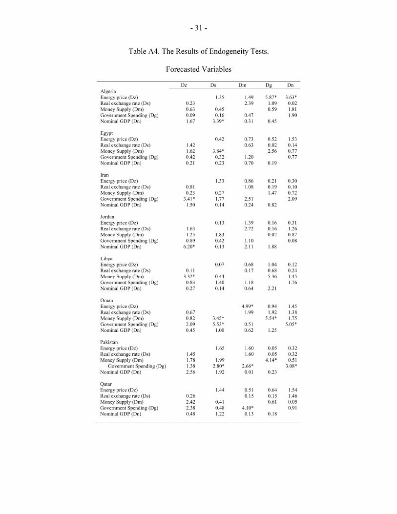
tv . We test for the endogeneity of the exchange-rate and the measures of aggregate demand and supply ( see Table A4). Given evidence of endogeneity, the forecast equations account for lagged values of variables proven to be statistically significant. Agents are expected to negotiate higher wages in anticipation of demand expansion. In turn, anticipated demand shifts are neutral.17 Nonetheless, anticipated demand shifts may determine real output through their effects on anticipated real exchange rate.18 Consequently, anticipated demand shifts may increase real output. Let zt be the log value of the energy price. Agents' expectation of a variable at time t based on information available at time t-1 is denoted by Et-1. Based on theory's forecast, output growth is expected to vary negatively with changes in the energy price, both anticipated and unanticipated, at time t-1. Accordingly, A1, A2 <0.19 Two sources of domestic policies, government spending and the money supply, approximate demand shifts, where gt and mt denote the log values of government spending and the money supply. Unanticipated growth in government spending and the money supply increase

16 Given the non-stationarity of the estimated dependent variables (see Table A1 for details), the empirical models are estimated in first-difference form. Hence, the anticipated component measures anticipated change in the policy variable. Shocks approximate unanticipated change (growth) in the policy variable. 17 In the real world, institutional rigidity may interfere with agents' ability to adjust fully to anticipated demand shifts. In the labor market, contracts may be longer than one year, preventing wages at time t from adjusting fully to anticipated demand shifts at time t-1. Accordingly, anticipated demand shifts are not absorbed fully in price. Alternatively, institutional rigidity may be attributed to price rigidity in the product market. To reduce menu costs, producers may resort to adjusting prices at specific intervals over time. Given price rigidity, anticipated demand shifts at time t-1 may determine real output growth in the short-run. For a discussion of the implications of sticky-wage and sticky-price models, see Kandil (1996). 18 Anticipated demand shifts increase price, increasing anticipated real exchange rate. This channel moderates anticipated increase in the real cost of imported intermediate goods, increasing the output supply. 19 The energy price is measured by the international energy price. For oil exporting countries, changes in oil price are likely to contribute positively to output growth. The increased capacity, following a rise in the energy price, is likely to moderate price inflation.

- 13 -

aggregate demand, creating positive price surprises. Hence, A4, A6>0. Anticipated growth in government spending and the money supply may also increase real output growth. Accordingly, A3, A5>0. Finally, anticipated appreciation of the real exchange rate determines the cost of the output supplied. Let rst be the log value of the real exchange rate.20 Based on Data availability, the exchange rate is measured by the real price of the domestic currency in U.S. Dollars. Graph 1 illustrates movements in the real exchange rate for various countries over time.21 Accordingly, a rise in the exchange rate indicates real appreciation of the domestic currency. As producers anticipate a lower cost of imported intermediate goods, in the face of currency appreciation, they increase the output supplied. Accordingly, A7>0. Unanticipated change in the exchange rate is likely, however, to determine both aggregate demand and supply22. Unanticipated currency appreciation, a positive shock to the exchange rate, decreases the cost of buying intermediate goods, increasing the output supplied. Concurrently, appreciation decreases net exports and the demand for domestic currency. The final effect remains indeterminate on aggregate demand, output, and price. To establish robustness, the empirical model in (15) is reestimated, replacing specific demand shifts (government spending and the money supply) with a broad measure of aggregate demand (nominal GDP or GNP) as follows:23

( )( ) ( )

0 1 1 2 1 3 1 4 1

5 1 6 1 7 1 8 1

9 1

( )t t t t t t t t t t t

t t t t t t t t t t

yt t

Dy A A E Dz A Dz E Dz A E Dn A Dn E Dn

A E Dg A Dg E Dg A E Drs A Drs E Drs

A EC v

− − − −

− − − −

−

= + + − + + −

+ + − + + − +

+

(16)

20 This measure captures shifts attributed to the nominal exchange rate, s, and the foreign price of imports, p*, in theory. 21 The forecast equation of the exchange rate is explained in the econometric methodology appendix. The forecast equation is based on a formal causality test in which we test the significance of lags of variables that may be relevant to the exchange rte. Hence, we do take into account the endogeneity of the exchange rate with respect to growth and inflation. Having accounted for the lags of all variables that are relevant to agents’ forecast, the shocks to the exchange rate are identified. 22 Unanticipated currency appreciation may be the result of unanticipated shock that moves the exchange rate relative to its expected value. Alternatively, unanticipated appreciation may be consistent with an overvalued currency compared to agents’ expectations that have adjusted downward in view of underlying macroeconomic fundamentals. 23 This measure is likely to vary with a variety of shocks underlying aggregate demand: the money supply, government spending, velocity, consumption, investment, and external shocks attributed to fluctuations in the current and capital accounts.

- 14 -

Here, nt denotes the log of the nominal value of Gross National or Domestic Product. This broad measure combines a variety of demand shifts stemming from the goods or money markets. Accordingly, A3>0, and A4>0. Model estimation will then determine how important exchange rate fluctuations are, given all other shocks impinging on the aggregate economy. To demonstrate fluctuations in the output price, an empirical model is specified as follows:

( )

( ) ( )0 1 1 2 1 3 1 4 1

5 1 6 1 7 1 1 9 1

( )t t t t t t t t t t t

t t t t t t t p t t t t

pt

Dp B B E Dz B Dz E Dz B E Dm B Dm E Dm

B E Dg B Dg E Dg B E Drs B Drs E Drs b EC

v

− − − −

− − − − −

= + + − + + −

+ + − + + − +

+

(17)

Based on test results, output price is evident to be non-stationary for the various countries under investigation. Accordingly, the empirical model is specified in first-difference form. Energy price shifts, both anticipated and unanticipated, increase the cost of the output produced and, hence, prices. Accordingly, B1, B2>0. Both anticipated and unanticipated demand shifts increase price inflation. Accordingly, B3, B4, B5, B6>0. Given the effect of anticipated currency appreciation in increasing the output supplied, price inflation decreases and B7<0.24 An unanticipated appreciation of the domestic currency (a positive shock to the exchange rate) increases the output supplied and may decrease (net exports effect) or increase (money demand effect) aggregate demand. The former two channels are deflationary while the latter increases price inflation. To establish robustness, the empirical model of price inflation is modified, replacing specific demand shifts with a broad measure of aggregate demand, nominal GNP/GDP shifts, as follows:

( )( )

0 1 1 2 1 3 1 4 1

7 1 8 1 9 1

( )t t t t t t t t t t t

pt t t t t t t

Dp B B E Dz B Dz E Dz B E Dn B Dn E Dn

B E Drs B Drs E Drs B EC v− − − −

− − −

= + + − + + −

+ + − + + (18)

Price inflation varies positively in the face of aggregate demand shifts, both anticipated and unanticipated. Accordingly, B3>0 and B4>0. Note that aggregate demand shifts are allocated between output growth in (16) and price inflation, in (18). Nonetheless, we

24 Anticipated shifts in the real exchange rate are function of lagged values of variables that enter the forecast equation, including its own lags. Hence, lagged values of domestic price are captured in anticipated currency shifts.

- 15 -

estimate a separate equation for price to test the effects of exchange rate fluctuations while controlling for a broad measure of aggregate demand in the empirical model.

IV. EMPIRICAL RESULTS

The results of estimating the empirical models of real output and price incorporating government spending and the money supply are presented in Table 1 for the sample of developing countries under investigation. These results indicate the effects of policy variables, as approximated by the monetary, fiscal and exchange rate shifts on output growth and price inflation. Table 2 contains the results of estimating the empirical models that incorporate nominal GNP or GDP as a proxy for aggregate demand. Table 3 contains summary statistics of the change in the real and nominal exchange rates, price inflation, and anticipated and unanticipated changes in the real exchange rate.

A. Fluctuations in the Face of Policy Shifts

Table 1 summarizes the evidence of estimating the empirical models in (15) and (17) for the various countries under investigation. Theory predicts that an increase in the energy price, both anticipated and unanticipated, increases the cost of the output produced. Hence, the output supplied decreases and price inflation increases. In oil-producing countries, however, an increase in the energy price is likely to cause an expansion in the output supplied and a reduction in price inflation. Anticipated and unanticipated changes in the energy price are generally insignificant on output and price in various countries.25 Theory predicts that agents adjust wages and prices in the face of anticipated monetary shifts, neutralizing their effects on output. Consistent with theory’s predictions, anticipated monetary shifts are insignificant in determining real output growth. The inflationary effect of anticipated monetary shifts is significant on price in four countries. Unanticipated monetary shifts are distributed between real output growth and price inflation with a coefficient that is dependent on the slope of the short-run supply curve. Output growth does not vary significantly in the face of unanticipated monetary shifts in any country. There is evidence, however, of an increase in price inflation in the face of unanticipated monetary growth in Egypt and Pakistan. Overall, the evidence indicates limited effects of monetary policy on real output growth in developing countries. Consistent with neutrality, anticipated government spending appears also insignificant on output growth in developing countries. Anticipated government spending does not accelerate price inflation significantly in any country. The inflationary effect of

25 It is worth noting that prices in many of the developing countries under investigation may be subject to controls that moderate or eliminate the effects of market shocks, as predicted by theory.

- 16 -

unanticipated government spending is evident and significant in Turkey. Overall, the real effect of fiscal policy is not significant to stimulate growth in developing countries. The exchange rate is measured by the real price of domestic currency in U.S. dollar. Accordingly, a rise in the exchange rate indicates real appreciation of the domestic currency.26 Theory predicts that anticipated appreciation in the value of the domestic currency decreases the cost of imported goods and increases output growth. There is no evidence of significant output growth in the face of exchange rate shifts in any country. Hence, the supply-side channel is not significant to transmit the effects of anticipated exchange rate shifts to the real economy. Nevertheless, there is significant evidence of an increase in price inflation in the face of anticipated exchange rage in Qatar.27 Unanticipated fluctuations of the domestic currency affect the demand and supply sides of the economy. A positive shock to the exchange rate (an unanticipated appreciation) increases the output supplied and decreases money demand and net exports. The first two channels cause output expansion, while the latter causes output contraction. In contrast, price inflation is likely to decrease with the increase in the output supplied and the reduction in net exports. Price inflation is likely to accelerate with the decrease in money demand. Output contraction is evident and significant in Jordan. Output expansion is evident and significant in Algeria. Hence, the evidence is not conclusive on the direction of the output response to unanticipated currency appreciation. Price inflation increases significantly in the face of unanticipated currency appreciation in Lybia and Qatar. Price inflation decreases significantly in the face of unanticipated currency appreciation in Algeria. Hence, the results are mixed concerning the inflationary effect of unanticipated currency appreciation.

B. Fluctuations in the Face of Aggregate Demand Shifts

Table 2 summarizes the evidence of estimating the empirical models in (16) and (18). Output contraction is evident and significant in the face of anticipated energy price increase in one country, where the inflationary effects are also significant. Output contraction is evident and significant in the face of unanticipated energy price increase in Egypt, Libya and Qatar. Price inflation is evident and significant in the face of unanticipated energy price increase in Egypt and Libya. Hence, the evidence remains robust concerning the limited effects of fluctuations in the energy price on economic performance in the sample of developing countries under investigation. 26 Throughout the paper, appreciation will describe increase in the foreign price of domestic currency attributed to either market forces or managed policy within a year. The estimation technique accounts for the endogeneity of the exchange rate with respect to domestic economic conditions. Exogenous shocks are attributed to domestic and/or external shocks. 27 Qatar is an oil producing country. Exchange rate appreciation may be consistent with an increase in capital inflation that stimulate price inflation.

- 17 -

Anticipated aggregate demand shifts are generally insignificant to stimulate output growth except in Iran and Jordan. In the remaining countries, the insignificant effects of anticipated demand shifts on real output growth support neutrality. Consistently, anticipated aggregate demand shifts increase price inflation significantly in Jordan, and Turkey. Evidence of significant price inflation appears also pervasive in the face of unanticipated aggregate demand shifts, as evident by the positive and significant response in Algeria, Iran, Pakistan, Syria, and Turkey. Evidence of significant output expansion in the face of unanticipated aggregate demand shifts is evident in Iran, Jordan, Pakistan, Syria and Turkey. Overall, the significant effects of aggregate demand shifts appear more pervasive compared to specific policy shifts. Hence, constraints on the demand side of the economy limit the transmission mechanism of specific policy shifts, namely fiscal and monetary, to the product market of many developing countries. Further, sources of spending do not appear to be closely tied to monetary or fiscal policies in many developing countries. Anticipated appreciation decreases price inflation and increases output growth significantly in Oman. Hence, the evidence remains robust concerning the limited effect of the supply-side channel in transmitting anticipated exchange rate shifts to the product market of the developing countries under investigation. Unanticipated exchange rate appreciation induces significant output expansion in Turkey. This evidence is consistent with the effect of currency appreciation in expanding the output supplied and decreasing money demand. Consistent with the effect of currency appreciation in decreasing net exports, output contraction is significant in Iran, Jordan, Libya, Oman, Qatar and Syria. Consistent with theory's predictions, the effects of unanticipated exchange rate fluctuations may be positive or negative on price inflation. Consistent with the reduction in money demand, price inflation increases significantly in the face of unanticipated currency appreciation in Jordan, Lybia, Oman and Qatar. Consistent with the increase in output supply and the reduction in net exports, price inflation decreases significantly in the face of unanticipated currency appreciation in Turkey. The mixed significant evidence provides further support for the complexity of demand and supply channels in determining the effects of exchange rate fluctuations on price inflation in many developing countries.

V. SUMMARY AND CONCLUSION

The analysis has focused on the effects of exchange rate fluctuations on a sample of 11 developing countries in the Middle East. To that end, the paper presents a theoretical rational expectation model that decomposes movements in the exchange rate into anticipated and unanticipated components. Anticipated changes in the exchange rate enter the production function through the cost of imported goods. Unanticipated currency fluctuations determine aggregate demand through exports, imports, and the demand for domestic currency, and determine aggregate supply through the cost of imported intermediate goods.

- 18 -

Let the exchange rate be the real price of the domestic currency in terms of a major international currency. Anticipated movements in the exchange rate are assumed to vary with agents' observations of macro-economic fundamentals determining changes in the exchange rate over time. A positive shock to the exchange rate, an unanticipated appreciation of the domestic currency, decreases net exports and money demand and increases the output supplied. Based on the strength of each channel, the combined effects of demand and supply channels may determine the direction of output and price adjustments in the face of currency fluctuations. In general, developing countries are characterized by a high degree of price flexibility in the face of aggregate demand shifts, both anticipated and unanticipated. Nonetheless, the real and inflationary effects of specific policy shocks, fiscal and monetary, appear limited on output and price. Hence, demand-side constraints block the transmission mechanism of domestic policies to the product market in many of the developing countries under investigation. Further, aggregate spending does not appear to be closely tied to monetary and fiscal policies in many developing countries. The limited effects of anticipated exchange rate appreciation on output growth and price inflation indicate that rational forecast of exchange rate movement is rather limited to gauge the strategy of agents in developing countries. Hence, producers do not adjust the supply side to react to a lower (higher) cost of imported goods in response to anticipated exchange rate appreciation (depreciation). In contrast, unanticipated fluctuations of the exchange rate appear more significant in determining fluctuations in output and price in many developing countries. Consistent with theory's predictions, output and price adjustments in the face of exchange rate shocks vary across countries. Consistent with the effects of unanticipated exchange rate appreciation (depreciation) in decreasing (increasing) net exports, output contraction (expansion) is evident and significant in six countries. Consistent with the effects of unanticipated exchange rate appreciation (depreciation) in increasing (decreasing) output supply and decreasing (increasing) money demand, output expansion (contraction) is evident and significant in two countries. Consistent with the effects of unanticipated currency appreciation (depreciation) in decreasing (increasing) net exports and increasing (decreasing) the output supplied, price inflation decreases (increases) significantly in two countries. Consistent with the effects of unanticipated currency appreciation (depreciation) in decreasing (increasing) money demand, price inflation increases (decreases) significantly in four countries. The results clearly illustrate the importance of designing exchange rate policy in consistency with agents’ forecasts, given underlying macroeconomic fundamentals. Movements in the exchange rate in consistency with agents’ expectations have limited effects on the macroeconomy. In contrast, high variability of exchange rate fluctuations around its anticipated value may generate adverse effects in the form of higher price inflation and larger output contraction in many developing countries. To minimize the

- 19 -

adverse effects of currency fluctuations, policy makers should aim at minimizing the dependency of the economy on foreign imports towards reducing fluctuations in the output supplied. While stimulating net exports through currency depreciation is desirable, it is crucial to ensure a concurrent increase in productive capacity to cope with the increased demand without accelerating price inflation. Relaxing constraints on the supply side are, therefore, necessary to reinforce output growth and stabilize prices in the face of currency fluctuations. Finally, monetary policy should aim at minimizing extensive fluctuations in the exchange rate that may induce speculative attacks and undermine the stability of the money demand function. Towards this objective, exchange rate policy should aim at striking the right balance between necessary flexibility to ensure competitiveness and desirable stability to increase confidence in domestic currency and underlying fundamentals that provide support to the currency value over time.

- 20 -

Table 1. Nonlinear 3SLS Parameter Estimates, using money supply and government spending Algeria Output A0 A1 A2 A3 A4 A5 A6 A7 A8 A9 RH0 0.17 -0.08 -0.03 0.24 0.003 -1.05 -0.002 -0.25 0.18 -0.52 0.29 (-0.47) (-0.50) (-0.82) (0.44) (0.02) (-0.88) (-0.02) (-0.54) (1.71) (-1.57) (1.29) R-square: 0.83 Price B0 B1 B2 B3 B4 B5 B6 B7 B8 B9 RH0 -0.17 0.28 0.24* -1.90 -0.06 3.55 0.83* 2.09 -0.38 -0.70* 0.57* (-0.25) (0.89) (3.11) (-1.06) (-0.17) (1.02) (2.61) (0.90) (-1.64) (-3.62) (3.73) R-square:0.91 Egypt Output A0 A1 A2 A3 A4 A5 A6 A7 A8 A9 RH0 0.05 0.24 -0.02 -0.04 0.09 -0.12 0.09 0.03 -0.06 -0.44 0.79** (0.61) (0.53) (-0.73) (-0.12) (0.73) (-0.23) (0.64) (0.04) (-1.12) (-1.08) (2.07) R-square:0.50 Price B0 B1 B2 B3 B4 B5 B6 B7 B8 B9 RH0 -0.02 -0.84 0.16 -0.08 0.68** 1.03 0.18 -1.90 -0.06 0.47 (-0.07) (-0.62) (1.75) (-0.10) (1.95) (0.58) (0.48) (-0.52) (-0.38) (1.35) R-square:0.57 Iran Output A0 A1 A2 A3 A4 A5 A6 A7 A8 A9 RH0 0.39 -0.89 -0.02 -1.59 -0.56 -0.05 -0.06 0.18 -0.15 0.64* (1.01) (-0.33) (-0.17) (-0.95) (-1.34) (-0.08) (-0.37) (0.62) (-1.24) (2.40) R-square: 0.55 Price B0 B1 B2 B3 B4 B5 B6 B7 B8 B9 RH0 0.23 0.94 -0.14 -0.03 0.26 -0.25 -0.41** 0.43 -0.15 0.34 (0.60) (0.30) (-1.18) (-0.02) (0.55) (-0.28) (-2.21) (1.17) (-0.99) (0.83) R-square: 0.22 Jordan Output A0 A1 A2 A3 A4 A5 A6 A7 A8 A9 RH0 0.03 -0.55 -0.05 0.35 -0.01 0.06 0.14 0.15 -0.41* -0.54 0.53 (0.43) (-0.78) (-1.30) (0.75) (-0.04) (0.36) (1.23) (0.35) (-4.32) (-1.80) (0.83) R-square: 0.86 Price B0 B1 B2 B3 B4 B5 B6 B7 B8 B9 RH0 0.05 -0.35 0.02 0.31** 0.14 -0.18 0.06 -0.10 0.14 0.27* 0.64** (1.46) (-0.71) (0.65) (2.18) (1.45) (-1.09) (1.02) (-1.21) (0.65) (3.38) (2.12) Libya Output A0 A1 A2 A3 A4 A5 A6 A7 A8 A9 RH0 -6.04 72.43 -0.0001 45.04 0.11 -1.22 0.12 -0.27 -0.002 0.23 (-0.01) (0.01) (-0.00) (0.01) (0.47) (-0.20) (0.85) (-0.81) (-0.02) (0.89) R-square:0.65 Price B0 B1 B2 B3 B4 B5 B6 B7 B8 B9 RH0 -9.05 129.41 0.12 87.67 0.09 -41.36 0.01 0.05 0.48* 0.57 (-0.01) (0.01) (1.60) (0.01) (0.37) (-0.03) (0.06) (0.09) (3.36) (1.27) R-square: 0.90

For parameter definitions, see notes at the end of Table 1.

- 21 -

Table 1. Nonlinear 3SLS Parameter Estimates, using money supply and government spending (continued)

Oman Output A0 A1 A2 A3 A4 A5 A6 A7 A8 A9 RH0 0.16 -0.27 0.34 -0.08 0.07 -0.72 0.24 1.89 -0.99 -0.33 (1.01) (-0.66) (1.54) (-0.09) (0.15) (-0.74) (0.68) (0.55) (-1.82) (-0.29) R-square: 0.78 Price B0 B1 B2 B3 B4 B5 B6 B7 B8 B9 RH0 0.02 -0.08 -0.05 0.41 -0.20 0.02 0.44 0.72 1.08 -0.02 -0.39 (0.18) (-0.30) (-0.23) (0.62) (-0.24) (0.02) (1.55) (0.36) (1.62) (-0.03) (-0.48) R-square: 0.96 Pakistan Output A0 A1 A2 A3 A4 A5 A6 A7 A8 A9 RH0 0.10 0.06 -0.01 -0.06 -0.01 -0.17 0.10 0.60 -0.07 -0.21 -0.33 (1.49) (0.28) (-0.61) (-0.26) (-0.07) (-0.79) (1.30) (0.43) (-0.60) (-0.60) (-0.29) R-square: 0.45 Price B0 B1 B2 B3 B4 B5 B6 B7 B8 B9 RH0 0.05 -0.06 0.01 0.39 0.55* 0.29 -0.01 1.33 0.29 -0.44 0.68 (0.48) (-0.19) (0.26) (1.38) (2.94) (1.06) (-0.13) (0.58) (1.49) (-1.07) (1.71) R-square: 0.31 Qatar Output A0 A1 A2 A3 A4 A5 A6 A7 A8 A9 RH0 0.12 0.05 0.20 -2.36 -0.07 0.17 -0.31 -0.11 -0.59 0.23 (0.52) (0.08) (0.97) (-0.48) (-0.34) (0.32) (-0.67) (-0.11) (-1.46) (0.69) R-square: 0.20 Price B0 B1 B2 B3 B4 B5 B6 B7 B8 B9 RH0 0.05 0.01 -0.01 -0.33 -0.003 0.01 0.03 1.11* 1.06* 0.83* (1.39) (0.20) (-0.64) (-0.52) (-0.20) (0.37) (0.91) (14.06) (38.12) (7.45) R-square: 0.99 Syria Output A0 A1 A2 A3 A4 A5 A6 A7 A8 A9 RH0 -0.11 -0.09 0.001 -0.46 0.27 1.43 0.07 0.02 -0.08 -0.96 (-0.47) (-0.15) (0.01) (-1.44) (0.47) (1.03) (0.31) (0.24) (-0.61) (-1.96) R-square: 0.42 Price B0 B1 B2 B3 B4 B5 B6 B7 B8 B9 RH0 -0.20 -0.06 -0.02 -0.50 -0.60 2.32 0.14 -0.15 -0.05 0.60 (-0.29) (-0.09) (-0.15) (-0.68) (-0.64) (0.58) (0.20) (-0.79) (-0.19) (1.31) R-square: 0.38 Tunisia Output A0 A1 A2 A3 A4 A5 A6 A7 A8 A9 RH0 0.03 -0.03 0.01 0.72 -0.24 -0.03 -0.05 1.85 0.04 0.07 -0.54 (0.27) (-0.35) (0.31) (1.34) (-1.16) (-0.12) (-0.48) (0.64) (0.27) (0.28) (-1.23) R-square:0.50 Price B0 B1 B2 B3 B4 B5 B6 B7 B8 B9 RH0 -0.03 0.12 -0.02 -0.74 -0.06 0.09 0.15 -1.86 -0.17 -0.04 0.98* (-0.02) (0.94) (-0.45) (-0.81) (-0.32) (0.75) (1.70) (-0.60) (-1.35) (-0.10) (3.00) R-square: 0.33

- 22 -

Table 1. Nonlinear 3SLS Parameter Estimates, using money supply and government spending (continued)

Turkey Output A0 A1 A2 A3 A4 A5 A6 A7 A8 A9 RH0 0.06 0.14 -0.05 -0.02 0.06 -0.02 -0.11 0.01 0.24** -0.13 (0.80) (0.34) (-1.05) (-0.08) (0.41) (-0.13) (-1.18) (0.02) (2.02) (-0.30) R-square: 0.39 Prices B0 B1 B2 B3 B4 B5 B6 B7 B8 B9 RH0 -0.60 3.87 0.01 0.66 -0.001 1.23* 0.70* 1.90 -0.35 0.79* (-0.85) (0.26) (0.19) (1.07) (-0.00) (2.91) (4.60) (0.79) (-1.89) (5.89) R-square: 0.89

A0 Intercept A1 Anticipated Energy Price A2 Unanticipated Energy Price A3 Anticipated Money Supply A4 Unanticipated Money Supply A5 Anticipated Government Spending A6 Unanticipated Government Spending A7 Anticipated Real Effective Exchange Rate A8 Unanticipated Real Effective Exchange Rate A9 Error Correction RH0 Serial correlation * Significant at 5%. ** Significant at 10%. t-ratios are in parentheses

- 23 -

Table 2. Nonlinear 3SLS Parameter Estimates, using nominal GDP

Algeria Output A0 A1 A2 A3 A4 A7 A8 A9 RH0 -0.02 -0.11** 0.06 0.21 -0.37* -0.40 -0.04 0.38* (-0.63) (-2.08) (1.68) (1.05) (-3.20) (-1.02) (-0.43) (2.52) R-square: 0.83 Price B0 B1 B2 B3 B4 B7 B8 B9 RH0 0.06 0.13* -0.04 0.50** 1.15* 0.36 -0.06 -0.13 0.24* (1.72) (2.73) (-1.25) (2.25) (10.99) (0.82) (-0.84) (-1.86) (4.18) R-square:0.99 Egypt Output A0 A1 A2 A3 A4 A7 A8 A9 RH0 -0.36 8.83 -

0.05** 0.50 -0.18 -0.28 -0.07 0.42*

(-0.04) (0.04) (-1.77) (0.46) (-1.64) (-0.50) (-1.43) (2.90) R-square: 0.42 Price B0 B1 B2 B3 B4 B7 B8 B9 RH0 0.19 -2.34 0.06* 0.15 1.10* 0.57 0.06 0.21* (0.41) (-0.23) (2.23) (0.11) (9.92) (0.46) (0.97) (3.67) R-square: 0.94 Iran Output A0 A1 A2 A3 A4 A7 A8 A9 RH0 -0.16 -0.68 0.04 0.99* 0.30* -0.17 -0.13* 0.45* (-1.64) (-0.69) (0.83) (2.56) (2.23) (-0.79) (-2.31) (2.21) R-square: 0.76 Price B0 B1 B2 B3 B4 B7 B8 B9 RH0 0.20 0.68 -0.06 -0.16 0.96* 0.42 0.04 0.31 -0.47 (1.40) (0.61) (-0.83) (-0.24) (5.07) (1.22) (0.51) (1.19) (-1.45) R-square: 0.70 Jordan Output A0 A1 A2 A3 A4 A7 A8 A9 RH0 0.02 -0.18 -0.02 0.35* 0.78* -0.14 -0.34* -0.02 -0.01 (0.67) (-0.43) (-0.96) (2.21) (3.81) (-0.99) (-6.21) (-0.18) (-0.07) R-square: 0.92 Price B0 B1 B2 B3 B4 B7 B8 B9 RH0 -0.03 0.29 -0.005 0.60* 0.30 0.20 0.43* -0.01 0.48** (-0.75) (0.56) (-0.24) (2.84) (1.29) (1.43) (5.82) (-0.04) (2.12) R-square: 0.90 Libya Output A0 A1 A2 A3 A4 A7 A8 A9 RH0 0.06 -0.13 -0.03 -0.68 0.37** -0.38 -0.28* 0.48* (0.90) (-1.81) (-0.61) (-0.63) (2.04) (-1.36) (-2.41) R-square:

0.78

Price B0 B1 B2 B3 B4 B7 B8 B9 RH0 -0.05 -0.02 0.08** -0.80 0.02 1.46* 0.78* 0.91* (-0.16) (-0.31) (1.77) (-0.85) (0.17) (2.31) (6.52) R-square: 0.85

For parameter definitions, see notes at the end of Table 2.

- 24 -

Table 2. Nonlinear 3SLS Parameter Estimates, using nominal GDP (continued)

Oman Output A0 A1 A2 A3 A4 A7 A8 A9 RH0 0.02 -0.09 0.14 0.35 0.47** -0.48 -0.83* 0.17 (0.29) (-0.69) (1.56) 0.68) 1.90) (-0.60) (-4.44) (0.78) R-square:0.83 Price B0 B1 B2 B3 B4 B7 B8 B9 RH0 -0.01 0.06 -0.03 0.53 0.40** 0.22 0.66* -0.29 0.42 (-0.32) (0.69) (-0.38) (1.45) (1.98) (0.39) (3.96) (-1.30) (1.03) R-square:0.98 Pakistan Output A0 A1 A2 A3 A4 A7 A8 A9 RH0 0.002 0.08 -0.01 0.48 0.16 0.43 -0.03 -0.19 0.37 (0.01) (0.43) (-0.56) (0.74) (0.94) (0.32) (-0.28) (-0.72) (1.12) R-square:0.29 Price

B0 B1 B2 B3 B4 B7 B8 B9 RH0 0.12 -0.10 -0.002 0.05 0.51** 1.17 0.20 -0.01 0.13 (0.78) (-0.50) (-0.13) (0.06) (1.79) (0.48) (1.41) (-0.04) (0.78) R-square:0.73 Qatar Output A0 A1 A2 A3 A4 A7 A8 A9 RH0 -0.05 0.40 -0.01 0.90 0.95* -0.84 -1.03* 0.04 0.04 (-

0.92) (0.98) (-

0.39) (1.48) (13.14) (-1.56) (-16.60) 0.94 (1.27)

R-square: 0.97 Price B0 B1 B2 B3 B4 B7 B8 B9 RH0 -0.01 0.02 0.004 0.37 0.02 1.15* 1.03* 1.00* (-

0.32) (0.48) (0.37) (0.65) (1.16) (3.36) (50.29) (6.68)

R-square:0.99

- 25 -

Table 2. Nonlinear 3SLS Parameter Estimates, using nominal GDP (continued)

Syria Output A0 A1 A2 A3 A4 A7 A8 A9 RH0 0.02 0.56 0.001 -0.14 0.20 -0.01 -0.13** -0.87* 0.85* (0.15) (0.35) (0.04) (-0.16) (1.21) (-0.06) (-2.16) (-2.47) (4.39) R-square:0.74 Price B0 B1 B2 B3 B4 B7 B8 B9 RH0 -0.14 0.66 -0.05 1.48 0.78* -0.08 -0.004 -0.26 (-0.78) (0.61) (-1.23) (1.28) (5.63) (-0.57) (-0.05) (-1.16) R-square: 0.70 Tunisia Output A0 A1 A2 A3 A4 A7 A8 A9 RH0 0.06 -0.04 0.01 0.07 0.46 0.80 0.05 -0.17 0.27 (0.54) (-0.64) (0.36) (0.18) (1.66) (0.22) (0.46) (-0.73) (0.87) R-square: 0.53 Price B0 B1 B2 B3 B4 B7 B8 B9 RH0 -0.07 0.28 -0.02 0.47 0.67 -2.23 -0.12 0.01 0.46 (-0.60) (1.30) (-0.63) (0.85) (1.78) (-0.66) (-0.87) (0.04) (1.45) R-square:0.72 Turkey Output A0 A1 A2 A3 A4 A7 A8 A9 RH0 0.08 0.50 -0.09* -0.14 0.16 -0.46 0.28* -0.14 (0.85) (0.32) (-2.16) (-1.07) (1.22) (-0.41) (2.41) (-0.35) R-square:0.28 Price B0 B1 B2 B3 B4 B7 B8 B9 RH0 -0.02 -0.13 0.10* 0.96* 1.04* 0.24 -0.34* 0.17 (-0.20) (-0.50) (2.44) (5.42) (7.35) (0.32) (-3.22) (1.57) R-square:0.89

A0 Intercept A1 Anticipated Energy Price A2 Unanticipated Energy Price A3 Anticipated nominal GDP A4 Unanticipated Nominal GDP A7 Anticipated Real Effective Exchange Rate A8 Unanticipated Real Effective Exchange Rate A9 Error Correction RH0 Serial correlation * Significant at 5%. ** Significant at 10%. t-ratios are in parentheses

- 26 -

Table 3. Summary Statistics of Exchange Rate and Price Inflation Data Mean Variance Min Max Algeria Real Exchange Rate (REX) -0.004 0.002 -0.11 0.08 Nominal Exchange Rate -0.04 0.004 -0.18 0.05 Price 0.06 0.002 -0.02 0.19 Predicted change in REX -0.02 0.001 -0.07 0.045 Unexpected change in REX -7.8E-06 0.01 -0.25 0.17 Predicted change in REX -0.001 0.002 -0.12 0.08 Unexpected change in REX 1.85E-06 0.006 -0.17 0.25 Egypt Real Exchange Rate (REX) -0.01 0.06 -0.32 0.06 Nominal Exchange Rate -0.03 0.01 -0.46 0.05 Price 0.05 0.001 0.09 0.15 Predicted change in REX -0.02 0.0004 -0.09 0.02 Unexpected change in REX 0.01 0.03 -0.72 0.17 Unexpected change in REX -0.01 0.05 -0.65 0.44 Iran Real Exchange Rate (REX) -0.01 0.01 -0.36 0.17 Nominal Exchange Rate -0.07 0.01 -0.36 0.04 Price 0.08 0.002 -0.02 0.21 Predicted change in REX -0.05 0.013 -0.22 0.20 Unexpected change in REX 0.02 0.05 -0.63 0.54 Jordan Real Exchange Rate (REX) 0.02 0.003 -0.06 0.25 Nominal Exchange Rate -0.01 0.002 -0.19 0.05 Price 0.03 0.001 -0.02 0.08 Predicted change in REX 0.04 0.0015 -0.11 0.12 Unexpected change in REX 0.001 0.014 -0.16 0.49 Libya Real Exchange Rate (REX) 0.01 0.003 -0.09 0.13 Nominal Exchange Rate -0.01 0.001 -0.08 0.05 Price 0.01 0.003 -0.09 0.13 Predicted change in REX 0.03 0.002 -0.05 0.11 Unexpected change in REX -0.003 0.015 -0.22 0.22

- 27 -

Table 3. Summary Statistics of Exchange Rate and Price Inflation Data (Continued) Mean Variance Min Max Oman Real Exchange Rate (REX) 0.0002 0.003 -0.12 0.12 Nominal Exchange Rate 0.001 0.0002 -0.04 0.04 Price 0.02 0.003 -0.01 0.17 Predicted change in REX -0.01 0.0005 -0.06 0.04 Unexpected change in REX 0.008 0.01 -0.25 0.26 Pakistan Real Exchange Rate (REX) -0.02 0.003 -0.25 0.06 Nominal Exchange Rate -0.03 0.003 -0.26 0.01 Price 0.04 0.0005 0.01 0.10 Predicted change in REX -0.03 0.0002 -0.05 0.02 Unexpected change in REX 0.01 0.004 -0.14 0.12 Qatar Real Exchange Rate (REX) 0.01 0.005 -0.13 0.20 Nominal Exchange Rate 0.004 0.0001 -0.004 0.04 Price 0.03 0.005 -0.12 0.22 Predicted change in REX 0.002 0.001 -0.09 0.09 Unexpected change in REX 0.01 0.02 -0.33 0.44 Syria Real Exchange Rate (REX) -0.01 0.01 -0.37 0.09 Nominal Exchange Rate -0.04 0.01 -0.46 0.01 Price 0.05 0.001 -0.003 0.11 Predicted change in REX -0.05 0.05 -0.59 0.35 Unexpected change in REX 0.01 0.04 -0.33 0.62 Tunisia Real Exchange Rate (REX) -0.01 0.001 -0.08 0.05 Nominal Exchange Rate -0.01 0.001 -0.09 0.05 Price 0.03 0.0002 0.008 0.06 Predicted change in REX -0.03 0.0002 -0.05 -0.0005 Unexpected change in REX -0.001 0.006 -0.17 0.12 Turkey Real Exchange Rate (REX) -0.004 0.003 -0.14 0.10 Nominal Exchange Rate -0.16 0.01 -0.43 0.02 Price 0.18 0.01 0.05 0.31 Predicted change in REX -0.02 0.001 -0.10 0.04 Unexpected change in REX 0.005 0.02 -0.28 0.27

- 28 -

Table A1. The KPSS Statistics for Null of Level Stationary. (The 5% critical value is 0.463)

Lag Truncation Parameter

0 1 2 3 4 Algeria Output 2.60 1.42 1.02 0.82 0.70 Price 2.33 1.25 0.88 0.70 0.59 Egypt Output 2.94 1.56 1.09 0.85 0.71 Price 2.74 1.43 0.99 0.77 0.64 Iran Output 2.02 1.12 0.82 0.68 0.60 Price 2.06 1.14 0.82 0.66 0.56 Jordan Output 2.89 1.52 1.06 0.83 0.69 Price 2.97 1.56 1.08 0.84 0.70 Libya Output 0.53 0.30 0.23 0.20 0.18 Price 2.19 1.20 0.86 0.70 0.60 Oman Output 2.97 1.56 1.08 0.84 0.70 Price 1.55 0.84 0.61 0.49 0.43 Pakistan Output 3.00 1.57 1.09 0.85 0.70 Price 2.73 1.45 1.01 0.80 0.60 Qatar Output 1.26 0.75 0.57 0.49 0.45 Price 2.06 1.14 0.83 0.67 0.58 Syria Output 2.80 1.49 1.04 0.89 0.69 Price 2.80 1.46 1.01 0.78 0.65 Tunisia Output 2.88 1.53 0.08 0.85 0.71 Price 3.00 1.57 1.08 0.84 0.70 Turkey Output 2.94 1.55 1.08 0.84 0.70 Price 1.16 0.70 0.54 0.47 0.43

Test description: The KPSS (Kwiatowski, Phillips, Schmidt, and Shin) stationarity test procedure examines the null hypothesis of stationarity of a univariate time series. The KPSS test assumes that a time series variable Xt could be decomposed into the sum of a deterministic trend, a random walk, and a stationary error. Then the random walk term is assumed to have two components: an anticipated component and an error term. Stationarity is established by testing if the variance of the error term is zero. If the calculated lag truncation variable is greater than 0.463, we reject the null hypothesis of stationarity.

- 29 -

Table A2. Cointegration Test Results ADF test statistics for the null hypothesis of non-stationary residuals.

Critical value at 10%=-2.62

Cointegration regression includes energy price, real exchange rate, money supply, and Government spending

Countries Output Price

Algeria -2.74* -2.69* Egypt -3.25* -2.32 Iran -1.17 -2.36 Jordan -3.33* -2.80* Libya -2.50 -0.72 Oman -1.53 -2.64* Pakistan -4.83* -4.74* Qatar -0.93 -1.21 Syria -2.00 -1.69 Tunisia -2.99* -2.67* Turkey -1.70 -1.82

Test Description: If we have n endogenous variables, each of which is first-order integrated (that is, each has a unit root or stochastic trend or random walk element), there can be from zero to n-1 linearly independent cointegrating vectors. If there is one cointegrating equation, the regression models of the text include a lag of error correction term.

To check for cointegration, we apply the ADF unit root test to the residual from the cointegration regression in which the non-stationary level of output and price are regressed on the level of variables that enter the model. * The results reject the null hypothesis of non-stationarity at the 10% level.

- 30 -

Table A3. Cointegration Test Results ADF Test statistics for the null hypothesis of non-stationary residuals,

Critical value at 10% =-2.62

Cointegration regression includes energy, price, real exchange rate , and nominal GDP

Countries Output Price

Algeria -2.35 -3.18* Egypt -2.13 -2.49 Iran -2.73* -2.57 Jordan -3.70* -2.76* Libya -1.87 -0.67 Oman -2.05 -4.44* Pakistan -4.78* -4.74* Qatar -3.23* -1.27 Syria -2.74* -2.40 Tunisia -0.73 -1.86 Turkey -1.62 -1.63

Test Description: If we have n endogenous variables, each of which is first-order integrated (that is, each has a unit root or stochastic trend or random walk element), there can be from zero to n-1 linearly independent cointegrating vectors. If there is one cointegrating equation, the regression models of the text include a lag of error correction term.

To check for cointegration, we apply the ADF unit root test to the residual from the cointegration regression in which the non-stationary level of output and price are regressed on the level of variables that enter the model. * The results reject the null hypothesis of non-stationarity at the 10% level.

- 31 -

Table A4. The Results of Endogeneity Tests.

Forecasted Variables

Dz Ds Dm Dg Dn Algeria Energy price (Dz) 1.35 1.49 5.87* 3.63* Real exchange rate (Ds) 0.23 2.39 1.09 0.02 Money Supply (Dm) 0.63 0.45 0.59 1.81 Government Spending (Dg) 0.09 0.16 0.47 1.90 Nominal GDP (Dn) 1.67 3.39* 0.31 0.45 Egypt Energy price (Dz) 0.42 0.73 0.52 1.53 Real exchange rate (Ds) 1.42 0.63 0.02 0.14 Money Supply (Dm) 1.62 3.84* 2.56 0.77 Government Spending (Dg) 0.42 0.32 1.20 0.77 Nominal GDP (Dn) 0.21 0.23 0.70 0.19 Iran Energy price (Dz) 1.33 0.86 0.21 0.30 Real exchange rate (Ds) 0.81 1.08 0.19 0.10 Money Supply (Dm) 0.23 0.27 1.47 0.72 Government Spending (Dg) 3.41* 1.77 2.51 2.09 Nominal GDP (Dn) 1.50 0.14 0.24 0.82 Jordan Energy price (Dz) 0.13 1.39 0.16 0.31 Real exchange rate (Ds) 1.63 2.72 0.16 1.26 Money Supply (Dm) 1.25 1.83 0.02 0.87 Government Spending (Dg) 0.89 0.42 1.10 0.08 Nominal GDP (Dn) 6.20* 0.13 2.11 1.88 Libya Energy price (Dz) 0.07 0.68 1.04 0.12 Real exchange rate (Ds) 0.11 0.17 0.68 0.24 Money Supply (Dm) 3.32* 0.44 5.36 1.45 Government Spending (Dg) 0.83 1.40 1.18 1.76 Nominal GDP (Dn) 0.27 0.14 0.64 2.21 Oman Energy price (Dz) 4.99* 0.94 1.45 Real exchange rate (Ds) 0.67 1.99 1.92 1.38 Money Supply (Dm) 0.82 3.45* 5.54* 1.75 Government Spending (Dg) 2.09 5.53* 0.51 5.05* Nominal GDP (Dn) 0.45 1.00 0.62 1.25 Pakistan Energy price (Dz) 1.65 1.60 0.05 0.32 Real exchange rate (Ds) 1.45 1.60 0.05 0.32 Money Supply (Dm) 1.78 1.99 4.14* 0.51

Government Spending (Dg) 1.38 2.80* 2.66* 3.08* Nominal GDP (Dn) 2.56 1.92 0.01 0.23 Qatar Energy price (Dz) 1.44 0.51 0.64 1.54 Real exchange rate (Ds) 0.26 0.15 0.15 1.46 Money Supply (Dm) 2.42 0.41 0.61 0.05 Government Spending (Dg) 2.38 0.48 4.10* 0.91 Nominal GDP (Dn) 0.48 1.22 0.13 0.18

- 32 -

Table A4. The Results of Endogeneity Tests. (Continued)

Forecasted Variables

Dz Ds Dm Dg Dn Syria Energy price (Dz) 0.27 0.99 2.47 Real exchange rate (Ds) 3.74* 1.60 1.65 Money Supply (Dm) 6.35* 0.52 7.87* Government Spending (Dg) 0.78 0.32 1.78 0.30 Nominal GDP (Dn) 0.26 1.22 0.17 1.39 Tunisia Energy price (Dz) 11.68* 3.82* 0.34 Real exchange rate (Ds) 1.43 2.40 0.23 Money Supply (Dm) 0.47 0.87 0.17 Government Spending (Dg) 0.62 2.09 0.75 1.56 Nominal GDP (Dn) 0.11 0.75 2.45 0.00 Turkey Energy price (Dz) 0.28 0.25 1.07 Real exchange rate (Ds) 1.10 0.21 0.95 Money Supply (Dm) 0.93 2.84* 1.27 Government Spending (Dg) 1.64 1.21 0.49 1.26 Nominal GDP (Dn) 0.89 0.46 2.08 0.80

* F-value is greater than the critical value of F at 10%.

- 33 -

Graph 1. Real Exchange Rates for 11 Middle Eastern Countries, 1971-2000.

0

5

10

15

20

25

1971

1974

1977

1980

1983

1986

1989

1992

1995

1998

Algeria

0

5

10

15

20

25

30

35

1971

1973

1975

1977

1979

1981

1983

1985

1987

1989

1991

1993

1995

1997

1999

Egypt

0

0.2

0.4

0.6

0.8

1

1.2

1.4

1971

1973

1975

1977

1979

1981

1983

1985

1987

1989

1991

1993

1995

1997

1999

Iran

0

10

20

30

40

50

60

70

80

90

1971

1973

1975

1977

1979

1981

1983

1985

1987

1989

1991

1993

1995

1997

1999

Jordan

0

10

20

30

40

50

60

70

80

1971

1973

1975

1977

1979

1981

1983

1985

1987

1989

1991

1993

1995

1997

1999

Libya

0

100

200

300

400

500

600

1971

1974

1977

1980

1983

1986

1989

1992

1995

1998

Oman

0

0.02

0.04

0.06

0.08

0.1

0.12

0.14

0.16

0.18

1971

1974

1977

1980

1983

1986

1989

1992

1995

1998

Pakistan

0

5

10

15

20

25

30

35

40

1971

1973

1975

1977

1979

1981

1983

1985

1987

1989

1991

1993

1995

1997

1999

Qatar

- 34 -

0

1

2

3

4

5

6

7

8

9

1971

1973

1975

1977

1979

1981

1983

1985

1987

1989

1991

1993

1995

1997

1999

Syria

0

20

40

60

80

100

120

140

160

1971

1974

1977

1980

1983

1986

1989

1992

1995

1998

Tunisia

0

0.05

0.1

0.15

0.2

0.25

1971

1974

1977

1980

1983

1986

1989

1992

1995

1998

Turkey

- 35 - APPENDIX I

ECONOMETRIC METHODOLOGY

The surprise terms that enter models (15) through (18) are unobservable, necessitating the construction of empirical proxies before estimation takes place. Thus, the empirical models include equations describing agents' forecast of aggregate or specific demand growth, the change in energy price, and the change in the real price of domestic currency in US dollar (the real exchange rate). All variables are first-differenced to render the series stationary, as described in Table A1. To decide on variables in the forecast equations, a formal causality test is followed. Each variable is regressed on two of its lags as well as two lags of all variables that enter the model: the change in the log value of the energy price, nominal GNP or GDP, the real exchange rate, government spending, and the money supply. The joint significance of the lags is tested for each variable (see Table A4). Accordingly, the forecast equations account for the lags of variables proven to be statistically significant. We test for structural break in the exchange rate. Given evidence of significant break, the forecast equation accounts for a dummy variable that captures significant changes in the means of the exchange rate as well its interaction with variables in the forecast equation. According to test results, significant structural break is evident in the exchange rate as follows Algeria (1988), Iran (1987), Libya (1989), Oman (1981), Pakistan (1982), Qatar (1981), Syria (1988), and Turkey (1981) Subtracting the above forecasts from the actual change in the variable results in surprises that enter the empirical model. In order to obtain efficient estimates and ensure correct inferences (i.e., to obtain consistent variance estimates), the empirical models are estimated jointly with a forecast equation for each anticipated regressor, following the suggestions of Pagan (1984 and 1986). To account for endogenous variables, instrumental variables are used in the estimation of the empirical models. The instrument list includes two lags of output, two lags of price, three lags of nominal GNP or GDP, 5 lags of the energy price, 5 lags of the real exchange rate, 5 lags of the money supply, and 5 lags of government spending. The paper's evidence remains robust with respect to modifications that alter variables or the lag length in the forecast equations and/or the instruments list. Following the suggestions of Engle (1982), the results of the test for serial correlation in simultaneous equation models are consistent with the presence of first-order autoregressive errors for some countries. To maintain comparability, it is assumed in all models that the error term follows an AR(1) process. The estimated models are transformed, therefore, to eliminate any possibility for serial correlation. The estimated residuals from the transformed models have zero means and are serially independent.

- 36 - APPENDIX II

DATA SOURCES

The sample period for investigation is 1971-2000. Annual data for the above countries are described as follows: 1. Real Output: Real output of GDP or GNP measured in terms of 1982 dollars.

2. The Price Level: The deflator for GDP or GNP.

3. The Energy Price: The price of Saudi Arabia oil.

4. Government Spending: Nominal values of all payments by the government. 5. Money Supply: the sum of currency plus demand deposits. 6. Real Exchange Rate: Real price of the domestic currency in U.S. dollar price, calculated

by multiplying the value of each country's currency in terms of the U.S. dollar (# of dollar per unit of the country's currency) by the country's price level and then dividing it by the U.S. price. A higher price represents appreciation of the currency. The U.S. consumer price index is taken from the Bureau of labor statistics web site, www.bls.gov.

Sources: 1 through 5 are taken from the World Economic Outlook, data bank available from the International Monetary Fund, Washington, D.C.

- 37 -

REFERENCES

Agenor, Pierre-Richard, 1991, “Output, Devaluation and the Real Exchange Rate in Developing Countries," Weltwirtschaftliches Archive, Band 127.

Bahmani, Mohsen, 1991, “Are Devaluation Contractionary in LDCs?” Journal of Economic

Development, (June). Barbone, Luca, and Francisco Rivera-Batiz, 1987, “Foreign Capital and the Contractionary

Impact of Currency Devaluation, with an Application to Jamaica," Journal of Development Economics, Vol. 26, (June), pp. 1–15.

Bruno, M., 1979, “Stabilization and Stagflation in a Semi-Industrialized Economy," in R.

Dornbusch and J. Frankel, eds. International Economic Policy, Johns Hopkins University Press, Baltimore, MD.

Buiter, William H., 1990, International Macroeconomics, Oxford University Press. Cooper, Richard N., 1971, “Currency Devaluation in Developing Countries," Essays in

International Finance, No. 86, International Finance Section, Princeton University. Diaz-Alejandro, Carlos F., 1963, “ Note on the Impact of Devaluation and Redistributive

Effect," Journal of Political Economy, Vol. 71, (August), pp. 577–80. Dornbusch, Rudiger, Open Economy Macroeconomics, 2nd edition, New York, 1988. Edwards, S., 1986, “Are Devaluation Contractionary?,” The Review of Economics and

Statistics, August. Engle, R. R., 1982, “A General Approach to Lagrange Multiplier Model Diagnostics,”

Journal of Econometrics, Vol. 20, pp. 83–104. Gylfason, Thorvaldur, and Schmid, Michael, ``Does Devaluation Cause Stagflation?"

Canadian Journal of Economics, Vol. XV1, November 1983. Gylfason, T. and Radetzki, 1991, “Does Devaluation Make Sense in Least Developed

Countries?" Economic Development and Cultural Change, (October). Guittian, Manuel, 1976, “The Effects of Changes in the Exchange Rate on Output, Prices,

and the Balance of Payments," Journal of International Economics, Vol. 6, pp. 65–74.

Hanson, James A., 1983, “Contractionary Devaluation, Substitution in Production and

Consumption, and the Role of the Labor Market," Journal of International Economics, Vol. 14, pp. 179–89.

-38-

Hirschman, Albert O., 1949, “Devaluation and the Trade Balance: A Note," Review of Economics and Statistics, Vol. 31, pp. 50–53.

Hoffmaister and Vegh, 1996, “Disinflation and the Recession Now Versus Recession Later

Hypothesis: Evidence from Uruguay," IMF Staff Papers, Vol. 43. Kandil, Magda, 1996, “Sticky Wage or Sticky Price? Analysis of the Cyclical Behavior of

the Real Wage,” Southern Economic Journal, (October), pp.440-99. Kandil, Magda, and Ida Mirzaie, 2002, “Exchange Rate Fluctuations and Disaggregated

Economic Activity in the U.S.: Theory and Evidence," Journal of International Money and Finance, No. 1, (February), pp. 1–31.

Kandil, Magda, and Ida Mirzaie, 2003, “The Effects of Dollar Appreciation on Sectoral

Labor Market Adjustments: Theory and Evidence," Quarterly Review of Economics and Finance, Vol. 43, No. 1, pp. 89–117.

Kandil, Magda, and Jeffrey Woods, 1997, “Cyclical Comovements in Industrial Labor and

Product Markets: Theory and Evidence," Economic Inquiry, Vol. XXXV, pp. 725–44. Kamin, and Rogers, 2000, “Output and the Real Exchange Rate in Developing Countries: An

Application to Mexico," Journal of Development Economics, No. 61. Krugman and Taylor, 1987, “Contractionary Effects of Devaluation," Journal of

International Economics, No. 8, pp. 445–56. Kwiatkowski, Denis, Peter C. B. Phillips, Peter Schmidt, and Yongcheol Shin, 1992,

“Testing the Null Hypothesis of Stationarity Against the Alternative of a Unit Root: How Sure Are We That Economic Time Series Have a Unit Root?" Journal of Econometrics, No. 54, pp. 159–78.

Lizondo, J. Saul, and Peter J. Montiel, 1989, ”Contractionary Devaluation in Developing

Countries: An Analytical Overview,” IMF Staff Papers, 36 (1), (March), pp. 182–227.

Meade, James E., 1951, The Theory of International Economic Policy, I: The Balance of

Payment, Oxford University Press, Oxford. Mendoza, E. G., 1992, “The Effect of Macroeconomic Shocks in a Basic Equilibrium

Framework," IMF Staff Papers, 39, 4, pp. 855–89. Pagan, Adrian, 1984, “Econometric Issues in the Analysis of Regressions with Generated

Regressors," International Economic Review, No. 25, pp. 221–47. Pagan, Adrian, 1986, “Two Stage and Related Estimators and Their Applications,” Review of

Economic Studies, No. 53, pp. 517–38.

-39-

Rogers, and Wang, 1995, “Output, Inflation, and Stabilization in a Small Open Economy:

Evidence from Mexico," Journal of Development Economics, No. 46. Shone, Ronald, 1989, “Open Economy Macroeconomics,” Harvester Wheatsheaf. Solimano, Andres, 1986, “Contractionary Devaluation in the Southern Cone-The Case of

Chile,” Journal of Development Economics, No. 23, pp. 135–51. Wijnbergen, Sweder Van, 1989, “Exchange Rate Management and Stabilization Policies in

Developing Countries," Journal of Development Economics, No. 23, pp. 227–47.