Comparative Advertising: disclosing horizontal matchinformation

Simon P. Anderson∗and Régis Renault�

October 2006; revised February 2009.

Abstract

Improved consumer information about horizontal aspects of products of similarquality leads to better consumer matching but also higher prices, so consumer surpluscan go up or down, while proÞts rise. With enough quality asymmetry though, thehigher quality (and hence larger) Þrm�s price falls with more information, so both effectsbeneÞt consumers. This is when comparative advertising is used, against a large Þrmby a small one. Comparative advertising, as it imparts more information, thereforehelps consumers. While it also improves proÞtability of the small Þrm, overall welfaregoes down because of the large loss to the attacked Þrm.Keywords: comparative advertising, information, product differentiation, quality.JEL ClassiÞcation: D42 L15 M37

Acknowledgement 1 We gratefully acknowledge travel funding from the CNRS andNSF under grant GA10273, and research funding under grant SES-0452864. We thankthe Editor and a referee for very constructive (and challenging!) comments, alongwith Federico Ciliberto, Joshua Gans, and Jura Liaukonyte. We thank Yoki Okawaand Öykü Ünal for research assistance, and various seminar participants (ToulouseI, ECARES-ULB, CORE-UCL, ENCORE, CENTER-Tilburg, Boston University, Royseminar in Paris, St. Andrews University, Pompeu-Fabreu, Melbourne Business School,University of Southern California, Claremont-McKenna, Virginia) and conference at-tendees (CESIfo 5th Area conference on Applied Micro in Munich and EARIE inOporto). We thank IDEI (University of Toulouse I), the University of Montpellier,Melbourne Business School, and the Portuguese-American Fund / Portuguese Compe-tition Authority (Lisbon) for their hospitality.

∗Department of Economics, University of Virginia, PO Box 400182, Charlottesville VA 22904-4128, USA.sa9w@virginia.edu

�ThEMA, Université de Cergy-Pontoise, 33 Bd. du Port, 95011, Cergy Cedex, FRANCE and InstitutUniversitaire de France. regis.renault@u-cergy.fr

1 Introduction

Until the late 1990s, mentioning a competitor�s brand in an ad was illegal in many EU coun-

tries. This situation was ended by a 1997 EU directive that made �comparative advertising�

legal subject to the restriction that it should not be misleading. This brought the European

approach closer to that of the FTC in the US. In other countries, comparative advertising re-

mains illegal, or little used (see Donthu, 1998, for a cross-country comparison). The rationale

for a favorable attitude towards �comparative advertising� on the part of competition au-

thorities is that it improves the consumers� information about available products and prices

(see Barigozzi and Peitz, 2005, for details and a wealth of examples and discussion). This

raises a number of questions for the economic analysis of informative advertising. What is

the scope of a practice that involves disclosing information that the product�s supplier would

choose not to reveal? Is the beneÞt to consumers from improved information mitigated by

a welfare loss for competitors who are (presumably) hurt by comparative advertising about

their products? Are consumers hurt by higher prices because product differentiation rises

due to comparative advertising about product attributes?

The FTC�s position is admirably clear: �Comparative advertising, when truthful and

non-deceptive, is a source of important information to consumers and assists them in making

rational purchase decisions.�1 This view underlies our modeling approach. The FTC also

expects performance beneÞts: �Comparative advertising encourages product improvement

and innovation, and can lead to lower prices in the marketplace.� To a very large extent we

corroborate these conclusions.

Here we consider a game between rival Þrms and their incentives to provide information.

Consumers do not know the characteristics of a Þrm�s product unless they are revealed

through advertising, although consumers have (correct) priors about their evaluations. Firms

1The STATEMENT OF POLICY REGARDING COMPARATIVE ADVERTISING by the Federal TradeCommission, of August 13, 1979, is to be found at http://www.ftc.gov/bcp/policystmt/ad-compare.htm

1

are fully aware of each other�s product attributes. If comparative advertising is illegal, then

Þrms can only inform consumers about their own goods. Comparative advertising allows a

Þrm to also inform consumers about rival product attributes that the other Þrm might not

wish to communicate. We also address the welfare economics of comparative advertising.

Evaluating the impact of comparative advertising requires identifying when it changes

the information available to consumers. That is, there must be some information that

Þrms would not disclose if restricted to direct advertising, and that will be brought out if

comparative advertising is allowed. In much of the literature on informative advertising, it

is the cost of advertising that limits the information transmission by Þrms (see the seminal

papers of Butters, 1977, Grossman and Shapiro, 1984, and the review coverage in Bagwell,

2007). Anderson and Renault (2006) show that a monopoly Þrm might limit information

about its product attributes even if advertising has no cost. This result is a starting point

for the present paper because it identiÞes situations where a Þrm is hurt by information

disclosure about its own product, so that there might be some incentives for competitors to

provide that information through comparative ads.

The paper contributes to the economics of asymmetric oligopolistic competition by Þrst

indicating how quality-cost advantages feed into equilibrium prices and sales. Second, it

provides results on the impact of increased product information on market outcomes: while

more information tends to increase proÞts, and welfare when qualities are similar, welfare can

be harmed with more information due to price distortions when qualities are quite different.

Third, it provides some predictions on when comparative advertising might be used � by

smaller Þrms with cost or quality disadvantages � and welfare implications.

There is curiously little economics literature on comparative advertising, although in

marketing there is quite a lot of documentation of the phenomenon and discussion of its

effectiveness (see Grewal et al., 1997, for a comprehensive survey).2 Barigozzi and Peitz

2A recent paper by Thompson and Hamilton (2006) shows subjects four different ads, with different

2

(2005) give a survey and some background modeling of alternative approaches.

Barigozzi, Garella, and Peitz (2006) take a signalling approach. An entrant with uncer-

tain quality confronts an incumbent whose quality is known. The entrant chooses between

�generic� advertising, which is standard money-burning to signal quality (as in Nelson, 1974),

and �comparative� advertising, which involves a claim comparing the two Þrms� qualities.

Firms may have favorable or unfavorable information about the entrant�s quality but do not

observe it perfectly. If comparative advertising is used, the incumbent may litigate in the

hope of obtaining damages if the court, which observes quality perfectly, Þnds that it is low.

Comparative advertising may credibly signal favorable information about entrant quality

when a Þrm with such information expects it unlikely a court will Þnd its quality is low.

Aluf and Shy (2001) model comparative advertising as shifting the transport cost to the

rival�s product in a Hotelling-type model of product differentiation. While this is an inter-

esting angle in its own right, the modeling approach does not capture the informative aspect

of comparison advertising and is not micro-founded in information revelation. Instead, it

seems more like a model of (negative) �persuasive� advertising. In a Hotelling-Downs model

of political competition, Harrington and Hess (1996) model negative political advertisements

as moving the rival�s perceived location away from the center, and positive advertisements

as moving one�s own perceived location towards the center (and hence increasing the chances

of being elected). They show that a candidate with a quality (valence) disadvantage will use

more negative advertising, in line with observed facts. Insofar as comparative advertising

in our model is information about a rival that the rival would rather not see revealed, this

result has an interesting parallel to our Þndings that a quality disadvantage is necessary for

comparative advertising.

We consider the disclosure of horizontally differentiated attributes (valued differently by

different consumers), assuming that product qualities are known. Here, product qualities are

comparative and analytical cues and judges ad effectiveness by surveying participants� impressions.

3

a device to indicate large or small Þrms in terms of their equilibrium market shares, and we

shall refer to the Þrms as strong (to be thought of as one with a quality advantage) or weak

(quality disadvantaged). If market sizes are very different (product qualities are sufficiently

different), the equilibrium to the disclosure game has only the weak Þrm disclosing horizontal

attributes and the strong one not. If comparative advertising is allowed, then the weak Þrm

will disclose the horizontal attributes of both products (and so it is truly comparative).

To see how the model works, it is Þrst useful to describe some background results which

nonetheless hold independent interest for the economics of product differentiation and infor-

mation. First, under Þrm symmetry, or close to it, more match information makes for more

product differentiation and therefore raises prices (as expected). As we show, consumers may

be better or worse off, as their improved ability to select the better match may be swamped

by the price hike. Nonetheless, Þrms are better off. Results are surprisingly different when

products are asymmetric, a case rarely treated by the literature. With zero horizontal match

information, Bertrand competition leads the weak Þrm to price at cost while the strong one

takes all the market by pricing at its quality advantage. Assume for the sequel this quality

advantage is large. If the match information for just one Þrm is known (the weak say), the

strong Þrm has to actually price lower to retain the whole market since it must attract the

consumer who likes the weak Þrm most. With full information, the strong Þrm must set an

even lower price if it is to retain (almost) all customers, since it must now attract the cus-

tomer who likes it least and likes its rival most.3 This means that not only are prices lower

when there is more information (more product differentiation) but also the strong Þrm�s

proÞts are lower the more information there is. However, the weak Þrm retains a foothold

under full information, so it prefers this.

This leads us into the advertising game analysis. Throughout the text we emphasize the

3We show that the strong Þrm will never want to completely price the rival out under full information,because the extra sales are not worth the lower price on infra-marginal units.

4

importance of Þrms� market shares by stressing two extreme cases, which allow for clean

analytical arguments. A speciÞc example helps Þll in intermediate cases.

Similarly sized Þrms share the same incentive to provide extensive horizontal match

information to maximize perceived differentiation and relax competition. Then, comparative

advertising has no speciÞc role insofar as full product information is provided regardless.

Dissimilar Þrms have quite different incentives to disclose horizontal match information.

Hence, allowing comparative advertising may have a signiÞcant impact. This is best illus-

trated when the match distribution is such that the lower market share falls to zero when

information is only one-sided:4 we show that shares are always positive with full informa-

tion. As noted above, the strong Þrm prefers no information to one-sided information, which

in turn it prefers to full information, and it serves the whole market unless its competitor

can achieve full information through comparative advertising. Hence, neither Þrm adver-

tises (provides information) when comparative advertising is banned (because the weaker

Þrm can get no market sales by using direct advertising for its own product alone). When

comparative advertising is allowed, the weaker Þrm will provide full product information to

give itself some market share (and hence proÞts).

If Þrms are sufficiently different, it is socially optimal that all consumers buy from the

stronger Þrm. Then, comparative advertising deteriorates social welfare by letting the weaker

Þrm make positive sales: full information relaxes the strong Þrm�s price incentive to capture

the whole market. Consumer welfare is improved though: full information brings down the

price of the strong product (which is otherwise consumed by all) and some consumers choose

to buy the cheap weak product which must therefore yield them higher surplus.

The text shows that these insights may remain valid even when the weak Þrm always

retains some strictly positive market share with one-sided information. Under fairly general

conditions, a sufficiently strong Þrm always prefers less information to more. We also show

4Technically, the condition is that the match density is strictly positive at the top of its support: f (b) > 0.

5

that there is a range of size differences for which the weak Þrm uses comparative advertising

to achieve full product information, which the strong Þrm prefers obscured.

These results indicate that the beneÞts of comparative advertising accrue to the weak Þrm,

and to consumers, with so much damage to the large Þrm that total surplus goes down. Al-

though we noted above that more information can raise prices (and may even hurt consumers

to the proÞt of Þrms, despite better consumer matching), this happens when comparative

advertising is irrelevant in the sense that incentives to divulge own product information are

already strong enough. When comparative advertising is relevant, the strong Þrm is at-

tacked by the weak one, and we are in the regime when more information actually reduces

prices (and enables better choices). This substantiates the FTC position that comparative

advertising improves competition, even though one might have worried a priori that more

match information would entail higher prices.

We provide an example with a Laplace distribution for match values with a complete

characterization of the equilibrium outcome and welfare properties as a function of Þrm

strengths. Results are fully consistent with those where the weak Þrm�s market share vanishes

to zero under one-sided information. This example shows that the weak Þrm�s proÞt can be

substantial enough to cover advertising expenses for comparative advertising.

Section 2 gives general background results for Bertrand duopoly with product differentia-

tion. We outline the model in Section 3, describe demand under different degrees of product

information, and Þnd the corresponding equilibrium prices. These prices and proÞts are

compared in Sections 4 and 5, which paves the way for the equilibrium information disclo-

sure determined in Section 6. Section 7 shows some key surplus properties on the desirability

of comparative advertising. Section 8 covers the Laplace example, and Section 9 discusses

quality revelation, other extensions, and interpretation of the model. Section 10 concludes.

The longer proofs are collected in the Appendix.

6

2 Some preliminary results

We Þrst give some results for duopoly pricing that are used quite extensively in the analy-

sis that follows: demands will satisfy the properties used here. The results pertain quite

generally to differentiated product Bertrand duopoly with covered markets.

Consider a duopoly where Þrms 0 and 1 set prices p0 and p1. DeÞne ∆ as Firm 1�s net

quality advantage, ∆ = p0 − p1 +Q, where Q ∈ IR may be understood as a Firm 1�s gross

quality advantage. Demand for Firm i�s product is given by Di(∆), i = 0, 1, where D1 is an

increasing function taking values in [0, 1] deÞned on IR. Further assume that D0 = 1−D1,which may be understood as a covered market assumption: if heterogenous consumers have

unit demands, each consumer must buy either product (and total demand is normalized to

1). Production costs are assumed to be zero.

Assume that D1(0) = D0(0) = 12so that, if Q = 0 and Þrms charge the same price, they

share demand equally. Thus, Q = 0 may be viewed as a symmetric case, whereas when

Q 6= 0, one Þrm has a competitive advantage over the other one in the sense that it may

charge a larger price than its competitor and still serve at least half the market (Firm 1

having the competitive advantage if Q > 0). This competitive advantage is presented for the

exposition as a quality difference, but could also be (and is formally equivalent to) a marginal

production cost difference (marginal costs being constant). To see this, simply reinterpret pi

as a mark-up over marginal cost. More generally the Þrm with the competitive advantage is

the one that has the larger difference between its quality and its marginal cost.5

We Þrst establish a general result characterizing Firm 1�s equilibrium net competitive

advantage, ∆, and how it relates to the gross competitive advantage Q.

5To see this, let c0 and c1 denote Þrms� (constant) marginal costs, and deÞne mi = pi − ci as Firmi�s mark-up. RedeÞne Q = (q1 − c1) − (q0 − c0) and set ∆ = m0 − m1 + Q. Then Firm 1�s proÞt isπ1 = m1D1 (∆) and now view Þrms as choosing their mark-ups. Hence the formal analysis is unaffected:note that ∆ = q1−p1−(q0 − p0) so that the demand functions are just as before. The advantaged Þrm is nowseen as the one with the higher quality-cost, and all results that follow can be appropriately re-interpreted.

7

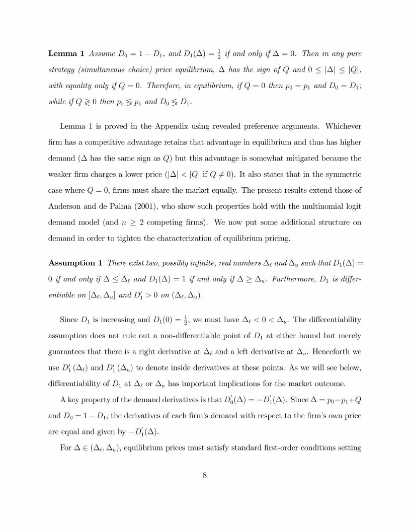
Lemma 1 Assume D0 = 1−D1, and D1(∆) = 12if and only if ∆ = 0. Then in any pure

strategy (simultaneous choice) price equilibrium, ∆ has the sign of Q and 0 ≤ |∆| ≤ |Q|,with equality only if Q = 0. Therefore, in equilibrium, if Q = 0 then p0 = p1 and D0 = D1;

while if Q ≷ 0 then p0 ≶ p1 and D0 ≶ D1.

Lemma 1 is proved in the Appendix using revealed preference arguments. Whichever

Þrm has a competitive advantage retains that advantage in equilibrium and thus has higher

demand (∆ has the same sign as Q) but this advantage is somewhat mitigated because the

weaker Þrm charges a lower price (|∆| < |Q| if Q 6= 0). It also states that in the symmetriccase where Q = 0, Þrms must share the market equally. The present results extend those of

Anderson and de Palma (2001), who show such properties hold with the multinomial logit

demand model (and n ≥ 2 competing Þrms). We now put some additional structure on

demand in order to tighten the characterization of equilibrium pricing.

Assumption 1 There exist two, possibly inÞnite, real numbers∆" and∆u such thatD1(∆) =

0 if and only if ∆ ≤ ∆" and D1(∆) = 1 if and only if ∆ ≥ ∆u. Furthermore, D1 is differ-entiable on [∆",∆u] and D0

1 > 0 on (∆",∆u).

Since D1 is increasing and D1(0) = 12, we must have ∆" < 0 < ∆u. The differentiability

assumption does not rule out a non-differentiable point of D1 at either bound but merely

guarantees that there is a right derivative at ∆" and a left derivative at ∆u. Henceforth we

use D01 (∆") and D

01 (∆u) to denote inside derivatives at these points. As we will see below,

differentiability of D1 at ∆" or ∆u has important implications for the market outcome.

A key property of the demand derivatives is thatD00(∆) = −D0

1(∆). Since∆ = p0−p1+Qand D0 = 1−D1, the derivatives of each Þrm�s demand with respect to the Þrm�s own priceare equal and given by −D0

1(∆).

For ∆ ∈ (∆",∆u), equilibrium prices must satisfy standard Þrst-order conditions setting

8

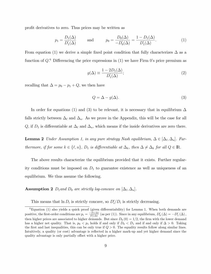
proÞt derivatives to zero. Thus prices may be written as

p1 =D1(∆)

D01(∆)

and p0 =D0(∆)

−D00(∆)

=1−D1(∆)D

01(∆)

. (1)

From equation (1) we derive a simple Þxed point condition that fully characterizes ∆ as a

function of Q.6 Differencing the price expressions in (1) we have Firm 0�s price premium as

g(∆) ≡ 1− 2D1(∆)D

01(∆)

; (2)

recalling that ∆ = p0 − p1 +Q, we then have

Q = ∆− g(∆). (3)

In order for equations (1) and (3) to be relevant, it is necessary that in equilibrium ∆

falls strictly between ∆" and ∆u. As we prove in the Appendix, this will be the case for all

Q, if D1 is differentiable at ∆" and ∆u, which means if the inside derivatives are zero there.

Lemma 2 Under Assumption 1, in any pure strategy Nash equilibrium, ∆ ∈ [∆",∆u]. Fur-thermore, if for some k ∈ {,, u}, D1 is differentiable at ∆k, then ∆ 6= ∆k for all Q ∈ IR.

The above results characterize the equilibrium provided that it exists. Further regular-

ity conditions must be imposed on D1 to guarantee existence as well as uniqueness of an

equilibrium. We thus assume the following.

Assumption 2 D1and D0 are strictly log-concave on [∆",∆u].

This means that lnDi is strictly concave, so D0i/Di is strictly decreasing.

6Equation (1) also yields a quick proof (given differentiability) for Lemma 1. When both demands arepositive, the Þrst-order conditions are pi =

−Di(∆)D0i(∆)

(as per (1)). Since in any equilibrium,D00 (∆) = −D0

1 (∆) ,

then higher prices are associated to higher demands. But since D0 (0) = 1/2, the Þrm with the lower demandhas a higher net quality. That is, p0 < p1 holds if and only if D0 < D1 and if and only if ∆ > 0. Takingthe Þrst and last inequalities, this can be only true if Q > 0. The equality results follow along similar lines.Intuitively, a quality (or cost) advantage is reßected in a higher mark-up and yet higher demand since thequality advantage is only partially offset with a higher price.

9

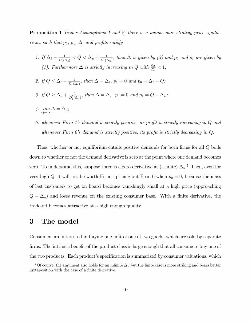
Proposition 1 Under Assumptions 1 and 2, there is a unique pure strategy price equilib-

rium, such that p0, p1, ∆, and proÞts satisfy

1. If ∆" − 1

D01(∆!)

< Q < ∆u +1

D01(∆u)

, then ∆ is given by (3) and p0 and p1 are given by

(1). Furthermore ∆ is strictly increasing in Q with d∆dQ< 1;

2. if Q ≤ ∆" − 1

D01(∆!)

, then ∆ = ∆", p1 = 0 and p0 = ∆" −Q;

3. if Q ≥ ∆u + 1

D01(∆u)

, then ∆ = ∆u, p0 = 0 and p1 = Q−∆u;

4. limQ→∞

∆ = ∆u;

5. whenever Firm 1�s demand is strictly positive, its proÞt is strictly increasing in Q and

whenever Firm 0�s demand is strictly positive, its proÞt is strictly decreasing in Q.

Thus, whether or not equilibrium entails positive demands for both Þrms for all Q boils

down to whether or not the demand derivative is zero at the point where one demand becomes

zero. To understand this, suppose there is a zero derivative at (a Þnite) ∆u.7 Then, even for

very high Q, it will not be worth Firm 1 pricing out Firm 0 when p0 = 0, because the mass

of last customers to get on board becomes vanishingly small at a high price (approaching

Q − ∆u) and loses revenue on the existing consumer base. With a Þnite derivative, thetrade-off becomes attractive at a high enough quality.

3 The model

Consumers are interested in buying one unit of one of two goods, which are sold by separate

Þrms. The intrinsic beneÞt of the product class is large enough that all consumers buy one of

the two products. Each product�s speciÞcation is summarized by consumer valuations, which

7Of course, the argument also holds for an inÞnite ∆u but the Þnite case is more striking and bears betterjuxtaposition with the case of a Þnite derivative.

10

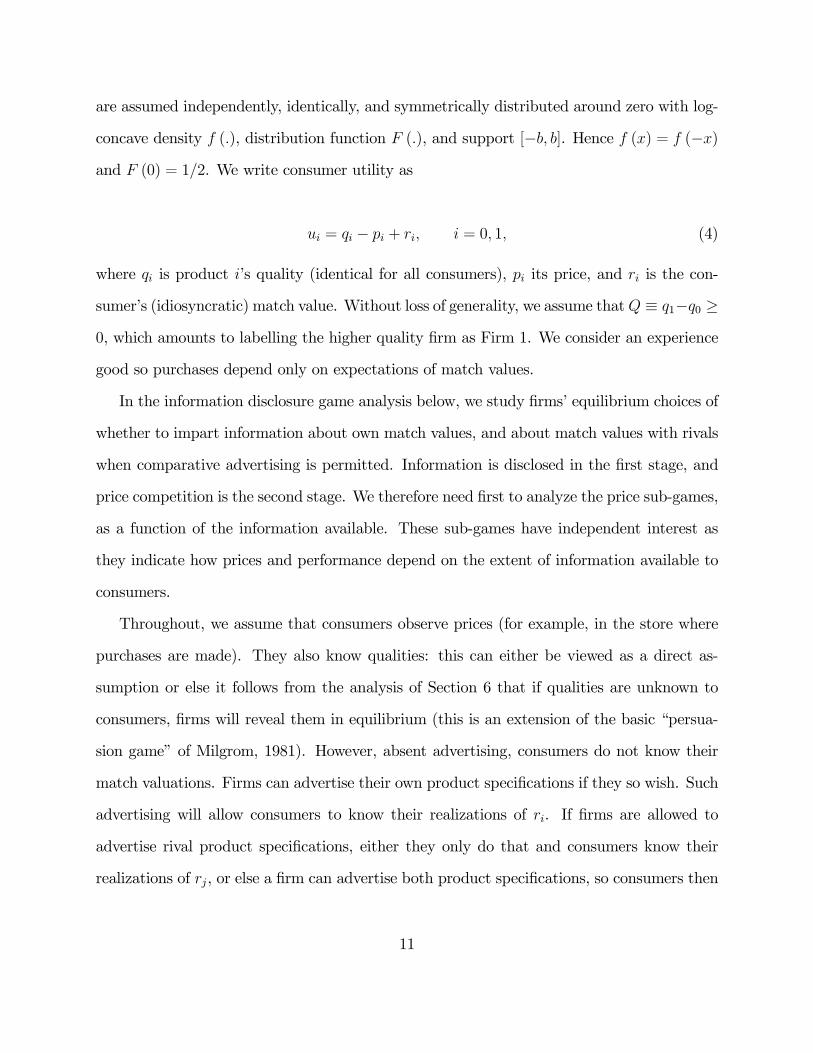
are assumed independently, identically, and symmetrically distributed around zero with log-

concave density f (.), distribution function F (.), and support [−b, b]. Hence f (x) = f (−x)and F (0) = 1/2. We write consumer utility as

ui = qi − pi + ri, i = 0, 1, (4)

where qi is product i�s quality (identical for all consumers), pi its price, and ri is the con-

sumer�s (idiosyncratic) match value. Without loss of generality, we assume thatQ ≡ q1−q0 ≥0, which amounts to labelling the higher quality Þrm as Firm 1. We consider an experience

good so purchases depend only on expectations of match values.

In the information disclosure game analysis below, we study Þrms� equilibrium choices of

whether to impart information about own match values, and about match values with rivals

when comparative advertising is permitted. Information is disclosed in the Þrst stage, and

price competition is the second stage. We therefore need Þrst to analyze the price sub-games,

as a function of the information available. These sub-games have independent interest as

they indicate how prices and performance depend on the extent of information available to

consumers.

Throughout, we assume that consumers observe prices (for example, in the store where

purchases are made). They also know qualities: this can either be viewed as a direct as-

sumption or else it follows from the analysis of Section 6 that if qualities are unknown to

consumers, Þrms will reveal them in equilibrium (this is an extension of the basic �persua-

sion game� of Milgrom, 1981). However, absent advertising, consumers do not know their

match valuations. Firms can advertise their own product speciÞcations if they so wish. Such

advertising will allow consumers to know their realizations of ri. If Þrms are allowed to

advertise rival product speciÞcations, either they only do that and consumers know their

realizations of rj, or else a Þrm can advertise both product speciÞcations, so consumers then

11

know both ri and rj, a situation we refer to as �comparative advertising.� Even though there

is nothing untruthful in comparative advertising, or in advertising a rival�s characteristics,

this may be information that Firm j may choose not to reveal on its own.8 If there is no

information on Firm i�s product speciÞcation (and hence the value of ri), consumers must

form expectations of their beneÞts from buying from Firm i. Consumers cannot otherwise

acquire any information through search.9 We next describe demand under the alternative

consumer information states that might arise from advertising.

3.1 No information

If neither Þrm advertises, the consumers know only the expected value from purchasing from

either of them. Since the mean match value is zero (by the assumption of symmetry of f),

expected utility is

ui = qi − pi.

Products are ex-ante homogenous except for the quality differential. Firm 1�s demand

is then zero if ∆ < 0, and one if ∆ > 0. If ∆ = 0, we invoke a standard tie-breaking rule

that assigns all demand to Firm 1: since we assume Q ≥ 0, this corresponds to an efficientallocation when Q > 0, and has no bite when Q = 0.

The price equilibrium under no information is quite straightforward. It follows from

a standard Bertrand equilibrium argument that the low quality Þrm sets a zero price in

equilibrium and the high-quality one serves the whole market at a price of Q.10 Since the

8And in that sense may be viewed as rather negative.9As shown in the online version, an alternative phrasing of the model with a search good instead of an

experience good, as in Wolinsky (1986) and Anderson and Renault (1999, 2000), gives rise to an equivalentformulation as long as the search cost is high enough.10Without further restriction, any price premium of Q with the price of the high quality Þrm between 0

and Q, is an equilibrium outcome to this game. Anderson and de Palma (1987) show that the equilibriumwe select is the unique limit of equilibria in a horizontally differentiated market, as product heterogeneitygoes to zero. This eliminates equilibria where the weak Þrm (which makes no sales) prices below marginalcost.

12

market size is normalized to unity, Q is also Firm 1�s equilibrium proÞt.

3.2 One-sided information

Here we characterize the demand (indicated with a bar) that ensues when the information

advertised concerns only one of the products (for example, only one Þrm advertises its

product speciÞcations). Suppose that Firm 0�s match is known. Then, since the expected

match value with Firm 1 is zero, the relevant utilities are

u0 = q0 − p0 + r0 and u1 = q1 − p1.

These expressions give rise to a demand facing Firm 1 given by Pr (u0 < u1) or

D1 = Pr (r0 < ∆) = F (∆) . (5)

Since the support of r0, the random variable underlying F (.), is [−b, b] we have here thatD1 (∆) = 1 for ∆ ≥ ∆u = b, and D1 (∆) = 0 for ∆ ≤ ∆l = −b, and Assumptions 1 and 2are satisÞed for this demand. Hence Proposition 1 holds.

We now argue the demands in such a situation are independent of which Þrm�s match

values are known (so the result is the same). Indeed, if Firm 1�s match is known and Firm

0�s match is unknown, the utilities relevant to choices are u0 = q0− p0 and u1 = q1− p1+ r1.The demand facing Firm 1 is then D1 = 1 − F (−∆). However, this demand expression isthe same as (5) since symmetry of f implies F (x) = 1− F (−x). In summary:

Lemma 3 If information is one-sided, each Þrm�s demand does not depend on which Þrm�s

match values are known.

Thus it makes no difference which Þrm�s matches are known (given only one Þrm�s are).

This means there is no systematic bias in the model to favor advertising one�s own match,

or one�s rival�s horizontal match.11

11This result depends on the symmetry of f . Skewness would bias the incentives to reveal or not.

13

Under one-sided information, from the analysis of Section 2, whether or not one Þrm is

excluded from the market in equilibrium depends on whether Q is high enough and whether

the derivative of demand is positive or zero at the upper bound. Since that derivative is

simply f (b) (where b = ∆u in the earlier notation), then we immediately have the following

result as a corollary to Lemma 2 and Proposition 1. Denote equilibrium values of variables

with an overbar.

Corollary 1 Suppose information is one-sided. Then equilibrium demands are both positive

regardless of Q if f (b) = 0. If f (b) > 0, then for Q ≥ b + 1f(b), Firm 1 serves the whole

market in equilibrium and sets a price p1 = Q − b while p0 = 0; for lower Q the market is

shared and p0, p1, and ∆ are given by equations (1)-(3). Lastly, ∆→ b as Q→∞.

Note that the case f (b) = 0 covers the case when the support of match values is the

extended real line. With a Þnite support and f (b) > 0, the quality-advantaged Þrm (1)

prices so as to just retain the individual enjoying the highest regard for Firm 0, which is the

individual who has a match r0 = b. This compares to the mean value of 0 for Firm 1.12

3.3 Full information

Consumers know exactly their match values with both products if they have been advertised.

Indeed, for what follows, it suffices that they only know the difference in values, r1− r0, thatis, the comparison between products. Arguably, this information might be easier to disclose

than an absolute match value.

A consumer with full information purchases product 1 if and only if

q1 − p1 + r1 ≥ q0 − p0 + r0

or equivalently r1 + ∆ ≥ r0. The probability a consumer with a realization r1 buys from

Firm 1 is F (r1 +∆). Integrating over all possible values of r1 gives Firm 1�s demand as12Equivalently, as per Lemma 3, Firm 1 must price so that the consumer least enamoured of it (holding

r1 = −b) nonetheless buys against an expected value of 0 with Firm 0.

14

eD1(∆) = Z b

−bF (r1 +∆) f (r1) dr1 (6)

and eD0(∆) = 1− eD1(∆), where full-information demands are characterized with a tilde.13The range of values of ∆ for which eD1(∆) is strictly between 0 and 1 is from ∆l = −2b

to ∆u = 2b, and Assumptions 1 and 2 are satisÞed for this demand. These bounds arise

because these are the values for which at least some value of F (r1 +∆) in (6) is neither zero

nor one. For example, if ∆ = 2b, even the consumer who least likes product 1 and most likes

product zero (that is, (r0, r1) = (b,−b), or, indeed, r0 − r1 = 2b) will just switch to buyingproduct 1 because its net quality advantage is so high.

Although this demand function has the whole market served by Firm 1 if ∆ ≥ 2b, thisnever happens in equilibrium. This property is a direct corollary of Lemma 2 and Proposition

1. Since for ∆ > 0 we can write (6) as eD1(∆) = R b−∆−b F (r1 +∆) f (r1) dr1 + 1− F (b−∆),then eD0

1(∆) =R b−∆−b f (r1 +∆) f (r1) dr1 and this expression is zero for ∆ = 2b. This puts us

always in Case 1 of Proposition 1, which proves the next point. Denote equilibrium values

with a tilde.

Corollary 2 Suppose full information prevails. Then equilibrium demands are positive re-

gardless of Q. Equivalently, the equilibrium ∆ (i.e., �∆) is always below 2b, and �p0, �p1, and

�∆ are given by equations (1)-(3). Lastly, �∆→ 2b as Q→∞.

Even though Firm 1 has the ability to price 0 out of the market, it never exercises the

option because the marginal gain in consumers is so small even when the stakes (the price)

are very large.

13By Lemma 1 we can concentrate on the case ∆ ≥ 0. Then (6) becomes �D1 (∆) =R b−∆−b F (r1 +∆) f (r1) dr1 + 1−F (b−∆). Demand can be visualized as the area of the unit square of con-sumer valuations accorded to each Þrm. The division line (indifferent consumer type) satisÞes r1 = r0 − �∆,which is a diagonal line. If �∆ > 0, Firm 1 attracts all those consumers for whom r0 < �∆ irrespective of theirvaluation of r1: hence the Þnal term in the demand function.

15

4 Equilibrium pricing for equal qualities

We now consider pricing sub-games conditional on information states induced by advertising

decisions in the Þrst stage of the game. Since the match density function, f , is log-concave,

arguments from Caplin and Nalebuff (1991) guarantee that Assumption 2 holds so that

existence and uniqueness under one-sided or full information follows from Proposition 1.

We Þrst compare equilibrium prices under symmetry of qualities (q0 = q1). If there is no

information, products are viewed as perfect substitutes and a standard Bertrand argument

gives prices both equal to marginal cost, which we recall is zero.

With one-sided information, demand for Firm 1 is given by (5) which, for Q = 0 yields

D1 = F (p0 − p1). Thus demand for Firm 0 is D0 = 1− D1 = 1−F (p0− p1). Using Lemma1, ∆ = 0; by Proposition 1, prices are equal (to 1/2D0 (0)) and are given by

p =1

2f (0). (7)

With full information, eD1 = R b−b F (p0 − p1 + r1) f (r1) dr1 (see (6)). Again fromCorollary2, both prices are equal to 1/2 eD0 (0), or

ep = 1

2R b−b f

2 (r) dr. (8)

These prices are compared below.

Proposition 2 If Q = 0, then �p ≥ p > 0, where the Þrst inequality is strict for distributionsother than the uniform. That is, prices are higher under full information than under one-

sided information than under no information.

Proof. Since f (.) is symmetric with maximum at r = 0, thenZ b

−bf2 (r) dr ≤ f (0)

Z b

−bf (r) dr = f (0) ,

16

or, from (7) and (8), p ≤ ep. Equality is only attained with a uniform density, so then prices

are equal. Otherwise, p < ep. Since demand is split 50�50, proÞts are also higher (unless f isuniform) under full information. Both prices exceed the no-information zero price.

With equal qualities, proÞts are simply equal to half the equilibrium prices. This makes

the case that more product information is better for Þrms (see also Meurer and Stahl, 1994).

Another way to think of this is to note that full information (when r1−r0 is known) is a meanpreserving spread of r1 alone (one-sided information), which in turn is a mean preserving

spread of 0 (no information). This progression reveals less product differentiation and hence

lower prices.

Full match information is the information state (for equal qualities) that gives the highest

total welfare. This is because there is no allocation distortion due to unequal prices, and full

information enables consumers to reach the Þrst-best solution that each consumer buys her

highest match.

The symmetric quality case underscores the product differentiation advantage imparted

by full information over limited information. However, the result that a higher degree of

information delivers higher equilibrium prices may lead to welfare losses if the model is

broadened to allow for non-purchase.14 This is one potential strike against the beneÞts of

informative advertising generally (and not just comparative advertising.)

In conclusion, a symmetric setting delivers no distinctive role for comparative advertising.

Nor does it enable much useful debate about the welfare beneÞts of comparative advertising.

For that, we turn to the case of quite different qualities. Note that results under symmetry

will hold in the neighborhood of Q = 0 since the various proÞt and surplus functions are

continuous and comparison inequalities are strict at Q = 0.15 This enables us below to state

14For another example, consumers might have price sensitive demands that depend also on their matchvalues. With full information, those that like the product a lot can buy a lot, and conversely: there is awelfare loss when there is less match information since "one-size Þts all" in demand.15Except for the uniform, where the price equality between one-sided and full information requires us to

evaluate explicitly what happens for Q > 0.

17

results for situations where Þrms are roughly of equal size.

5 Asymmetric qualities and information states

We Þrst establish a (non-equilibrium) result which will be used later for the asymmetric

cases, and helps build intuition for the results. The expressions compared are demands

under full and one-sided information (see (5) and (6)) for given prices.16

Proposition 3 The Þrm with higher net quality has higher quantity demanded under one-

sided information than full information:

eD1 (∆) = Z b

−bF (r1 +∆)f(r1)dr1 ≤ F (∆) = D1 (∆)

if and only if ∆ ≥ 0, with equality if and only if ∆ = 0.

One-sided information gives a demand advantage to the Þrm with a net quality advantage

because consumers impute the average valuation (0) to the unknown match value. The

situation can also be interpreted as that of a monopolist facing a (known) outside option: a

"strong" monopolist will therefore prefer not to advertise speciÞc match values. This insight

underpins results in Anderson and Renault (2006) where high search costs play effectively the

role of an attractive outside option (so the monopolist is more likely to want to advertise).

The result also suggests that were we to allow more Þrms, strategic effects aside, lower quality

ones are more likely to wish to prefer fuller information. We return to this point below.

While the Proposition suggests that Firm 1 is better off when information is one-sided

because it has higher demand for given ∆ > 0, it is less clear whether the equilibrium ∆

also favors it, since one might also suspect that it could support a higher price under full

16This inequality is related to Jensen�s inequality. We compare the expected value of some functionaltransformation of a random variable with the value of that function evaluated at the expected value of therandom variable; Jensen�s inequality compares these quantities under a convexity assumption on the func-tional whereas we consider a functional that is Þrst convex and then concave. For the uniform distribution,F (r+∆) is piecewise linear and a quick proof of the result may be obtained by applying Jensen�s inequality.

18

information insofar as this means greater perceived product differentiation. The proÞt results

are proved next, Þrst determining the effect on proÞt of rival price and then own price.

For the next two results, a strong demand state refers to the information state (i.e., full

information or one-sided information) for which a Þrm�s demand is higher for all ∆, given

the advantage conferred by Proposition 3. Let �πi and πi, i = 0, 1 denote a Þrm�s equilibrium

proÞt under full and one-sided information respectively.

Lemma 4 Assume Q > 0. A Þrm�s proÞt in its strong demand state is strictly higher than

in its weak demand state if its rival�s equilibrium price is higher in the strong state. Hence:

1. if �p1 ≥ p1 then �π0 > π0.

2. if p0 ≥ �p0 then π1 > �π1.

Proof. First assume that �p1 ≥ p1. Under full information, Firm 0 can always select a

price such that ∆ = ∆ so that, by Proposition 3 and since ∆ > 0 for Q > 0, its demand is

higher than with one-sided information. Furthermore, the corresponding price is p0+�p1−p1 ≥p0 so that its proÞt is strictly higher than with one-sided information. A symmetric argument

shows the other part of the Lemma.

Intuition for this lemma is simple. In either informational state, our model has the

standard property that a Þrm may achieve higher proÞts if its rival charges a higher price

because the Þrm can achieve the same price difference and hence the same demand while

charging a higher price. If in addition the state at which the rival�s price is higher coincides

with that at which demand is higher at any given price difference, then that state is clearly

more proÞtable. However, a fundamental tension is that rivals may charge lower prices in

Þrms� strong states, meaning that we have to go deeper into the model to resolve Þrms�

information revelation incentives, which we do in the next lemma and the next section.

19

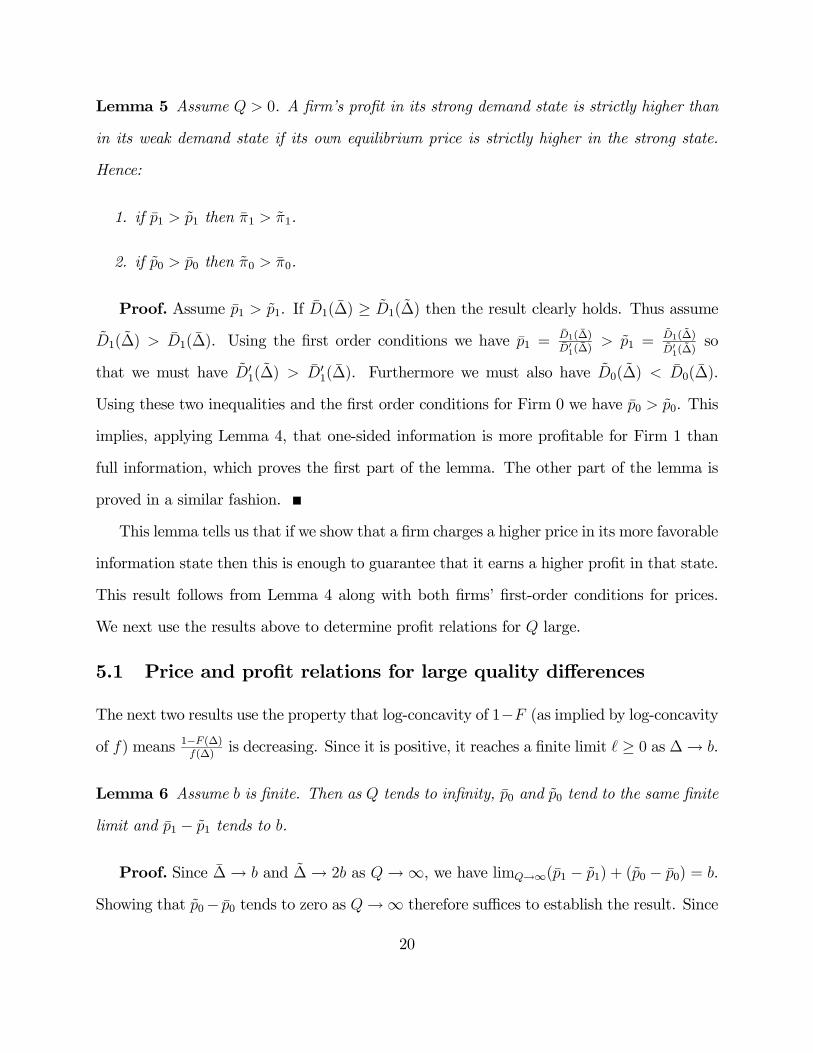
Lemma 5 Assume Q > 0. A Þrm�s proÞt in its strong demand state is strictly higher than

in its weak demand state if its own equilibrium price is strictly higher in the strong state.

Hence:

1. if p1 > �p1 then π1 > �π1.

2. if �p0 > p0 then �π0 > π0.

Proof. Assume p1 > �p1. If D1(∆) ≥ �D1( �∆) then the result clearly holds. Thus assume

�D1( �∆) > D1(∆). Using the Þrst order conditions we have p1 =D1(∆)D01(∆)

> �p1 =�D1( �∆)�D01(�∆)so

that we must have �D01( �∆) > D0

1(∆). Furthermore we must also have �D0( �∆) < D0(∆).

Using these two inequalities and the Þrst order conditions for Firm 0 we have p0 > �p0. This

implies, applying Lemma 4, that one-sided information is more proÞtable for Firm 1 than

full information, which proves the Þrst part of the lemma. The other part of the lemma is

proved in a similar fashion.

This lemma tells us that if we show that a Þrm charges a higher price in its more favorable

information state then this is enough to guarantee that it earns a higher proÞt in that state.

This result follows from Lemma 4 along with both Þrms� Þrst-order conditions for prices.

We next use the results above to determine proÞt relations for Q large.

5.1 Price and proÞt relations for large quality differences

The next two results use the property that log-concavity of 1−F (as implied by log-concavityof f) means 1−F (∆)

f(∆)is decreasing. Since it is positive, it reaches a Þnite limit , ≥ 0 as ∆→ b.

Lemma 6 Assume b is Þnite. Then as Q tends to inÞnity, p0 and �p0 tend to the same Þnite

limit and p1 − �p1 tends to b.

Proof. Since ∆→ b and �∆→ 2b as Q→∞, we have limQ→∞(p1 − �p1) + (�p0 − p0) = b.Showing that �p0− p0 tends to zero as Q→∞ therefore suffices to establish the result. Since

20

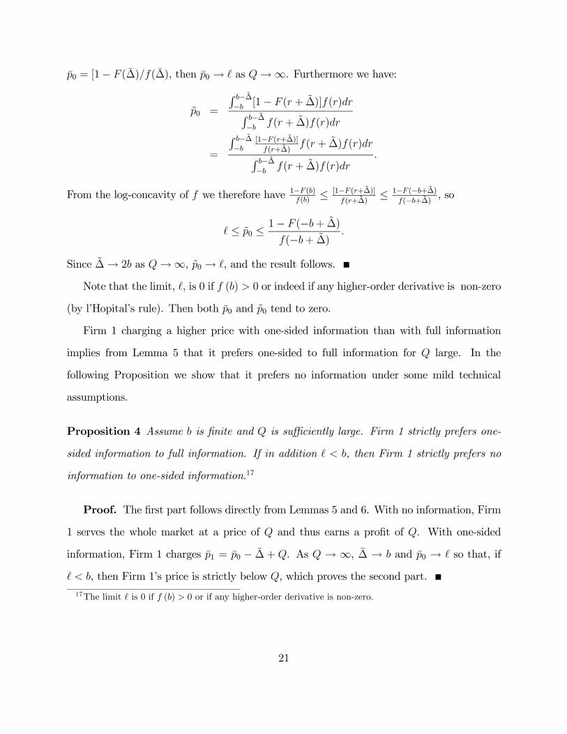
p0 = [1− F (∆)/f(∆), then p0 → , as Q→∞. Furthermore we have:

�p0 =

R b− �∆−b [1− F (r + �∆)]f(r)drR b− �∆

−b f(r + �∆)f(r)dr

=

R b− �∆−b

[1−F (r+�∆)]f(r+�∆)

f(r + �∆)f(r)drR b− �∆−b f(r + �∆)f(r)dr

.

From the log-concavity of f we therefore have 1−F (b)f(b)

≤ [1−F (r+�∆)]f(r+�∆)

≤ 1−F (−b+�∆)f(−b+�∆) , so

, ≤ �p0 ≤ 1− F (−b+ �∆)

f(−b+ �∆).

Since �∆→ 2b as Q→∞, �p0 → ,, and the result follows.

Note that the limit, ,, is 0 if f (b) > 0 or indeed if any higher-order derivative is non-zero

(by l�Hopital�s rule). Then both p0 and �p0 tend to zero.

Firm 1 charging a higher price with one-sided information than with full information

implies from Lemma 5 that it prefers one-sided to full information for Q large. In the

following Proposition we show that it prefers no information under some mild technical

assumptions.

Proposition 4 Assume b is Þnite and Q is sufficiently large. Firm 1 strictly prefers one-

sided information to full information. If in addition , < b, then Firm 1 strictly prefers no

information to one-sided information.17

Proof. The Þrst part follows directly from Lemmas 5 and 6. With no information, Firm

1 serves the whole market at a price of Q and thus earns a proÞt of Q. With one-sided

information, Firm 1 charges p1 = p0 − ∆ + Q. As Q → ∞, ∆ → b and p0 → , so that, if

, < b, then Firm 1�s price is strictly below Q, which proves the second part.

17The limit 2 is 0 if f (b) > 0 or if any higher-order derivative is non-zero.

21

What this means is that the quality advantaged Þrm may want to hold back information

and keep consumers uninformed.18 Nevertheless, the other Þrm�s incentives may lie in the

opposite direction. As shown next, this would happen if the density f is differentiable at b.

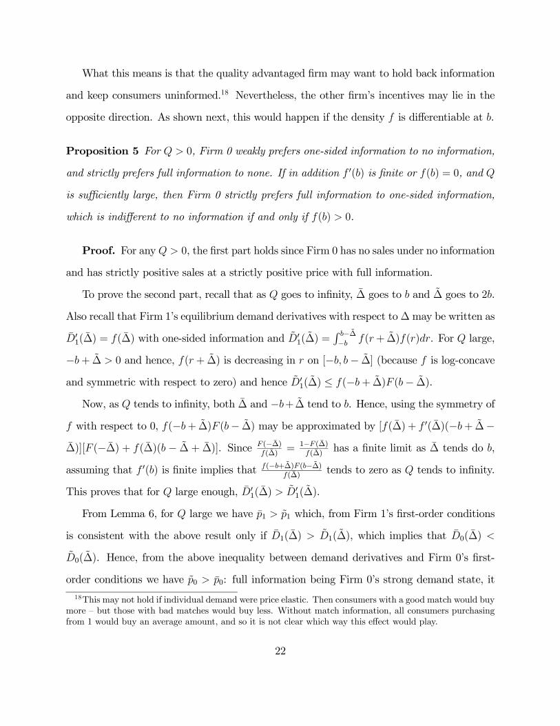
Proposition 5 For Q > 0, Firm 0 weakly prefers one-sided information to no information,

and strictly prefers full information to none. If in addition f 0(b) is Þnite or f(b) = 0, and Q

is sufficiently large, then Firm 0 strictly prefers full information to one-sided information,

which is indifferent to no information if and only if f(b) > 0.

Proof. For anyQ > 0, the Þrst part holds since Firm 0 has no sales under no information

and has strictly positive sales at a strictly positive price with full information.

To prove the second part, recall that as Q goes to inÞnity, ∆ goes to b and �∆ goes to 2b.

Also recall that Firm 1�s equilibrium demand derivatives with respect to∆may be written as

D01(∆) = f(∆) with one-sided information and �D

01( �∆) =

R b− �∆−b f(r+ �∆)f(r)dr. For Q large,

−b+ �∆ > 0 and hence, f(r + �∆) is decreasing in r on [−b, b− �∆] (because f is log-concave

and symmetric with respect to zero) and hence �D01( �∆) ≤ f(−b+ �∆)F (b− �∆).

Now, as Q tends to inÞnity, both ∆ and −b+ �∆ tend to b. Hence, using the symmetry off with respect to 0, f(−b+ �∆)F (b− �∆) may be approximated by [f(∆) + f 0(∆)(−b+ �∆−∆)][F (−∆) + f(∆)(b − �∆ + ∆)]. Since F (−∆)

f(∆)= 1−F (∆)

f(∆)has a Þnite limit as ∆ tends do b,

assuming that f 0(b) is Þnite implies that f(−b+�∆)F (b− �∆)f(∆)

tends to zero as Q tends to inÞnity.

This proves that for Q large enough, D01(∆) > �D0

1( �∆).

From Lemma 6, for Q large we have p1 > �p1 which, from Firm 1�s Þrst-order conditions

is consistent with the above result only if D1(∆) > �D1( �∆), which implies that D0(∆) <

�D0( �∆). Hence, from the above inequality between demand derivatives and Firm 0�s Þrst-

order conditions we have �p0 > p0: full information being Firm 0�s strong demand state, it

18This may not hold if individual demand were price elastic. Then consumers with a good match would buymore � but those with bad matches would buy less. Without match information, all consumers purchasingfrom 1 would buy an average amount, and so it is not clear which way this effect would play.

22

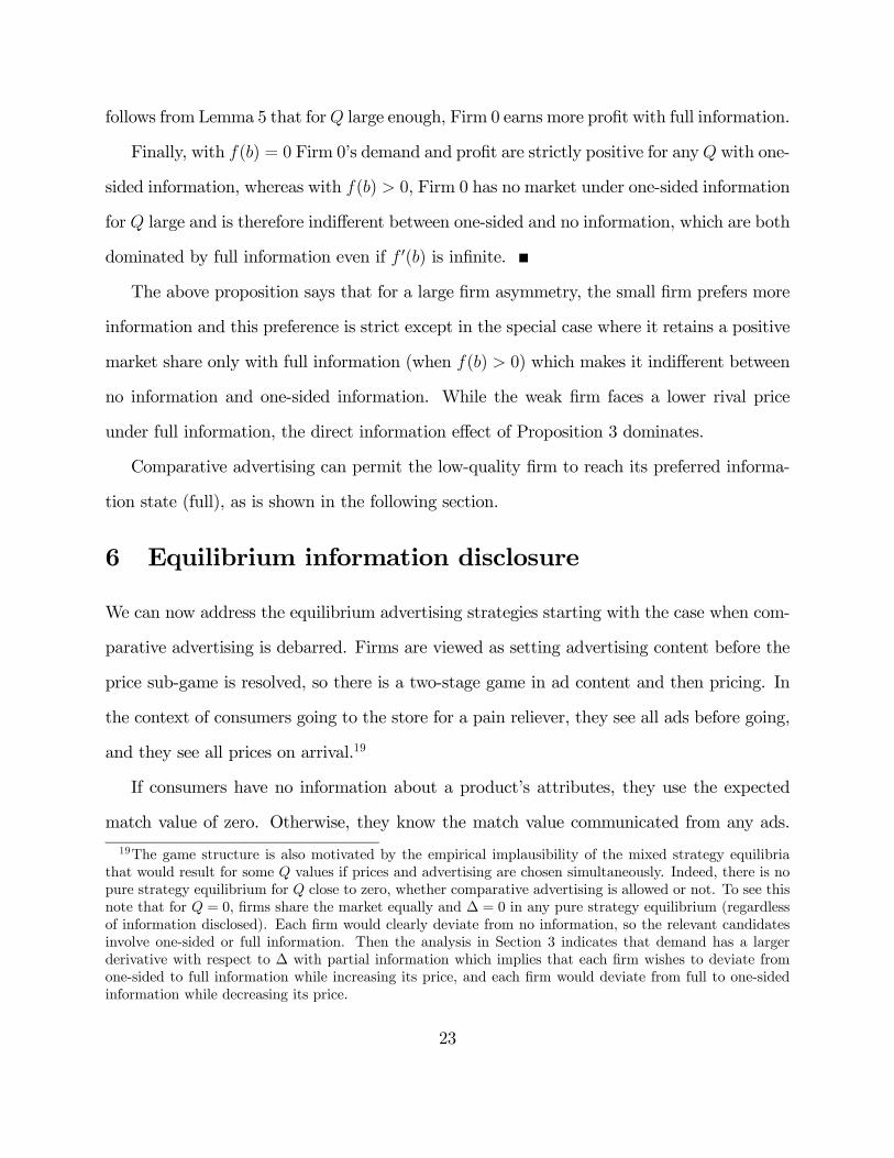
follows from Lemma 5 that forQ large enough, Firm 0 earns more proÞt with full information.

Finally, with f(b) = 0 Firm 0�s demand and proÞt are strictly positive for anyQ with one-

sided information, whereas with f(b) > 0, Firm 0 has no market under one-sided information

for Q large and is therefore indifferent between one-sided and no information, which are both

dominated by full information even if f 0(b) is inÞnite.

The above proposition says that for a large Þrm asymmetry, the small Þrm prefers more

information and this preference is strict except in the special case where it retains a positive

market share only with full information (when f(b) > 0) which makes it indifferent between

no information and one-sided information. While the weak Þrm faces a lower rival price

under full information, the direct information effect of Proposition 3 dominates.

Comparative advertising can permit the low-quality Þrm to reach its preferred informa-

tion state (full), as is shown in the following section.

6 Equilibrium information disclosure

We can now address the equilibrium advertising strategies starting with the case when com-

parative advertising is debarred. Firms are viewed as setting advertising content before the

price sub-game is resolved, so there is a two-stage game in ad content and then pricing. In

the context of consumers going to the store for a pain reliever, they see all ads before going,

and they see all prices on arrival.19

If consumers have no information about a product�s attributes, they use the expected

match value of zero. Otherwise, they know the match value communicated from any ads.

19The game structure is also motivated by the empirical implausibility of the mixed strategy equilibriathat would result for some Q values if prices and advertising are chosen simultaneously. Indeed, there is nopure strategy equilibrium for Q close to zero, whether comparative advertising is allowed or not. To see thisnote that for Q = 0, Þrms share the market equally and ∆ = 0 in any pure strategy equilibrium (regardlessof information disclosed). Each Þrm would clearly deviate from no information, so the relevant candidatesinvolve one-sided or full information. Then the analysis in Section 3 indicates that demand has a largerderivative with respect to ∆ with partial information which implies that each Þrm wishes to deviate fromone-sided to full information while increasing its price, and each Þrm would deviate from full to one-sidedinformation while decreasing its price.

23

Recall that advertising is costless. We start with close qualities.

Proposition 6 If Q > 0 is small enough and comparative advertising is barred, then each

Þrm reveals its match in the only equilibrium. This is still an equilibrium when comparative

advertising is allowed.

Proof. For Q = 0, for any distribution apart from the uniform, from Proposition 2, each

Þrm�s proÞt is strictly higher when it reveals information than when it does not, regardless

of the strategy of the other Þrm. By continuity, this property still holds for Q > 0 small

enough, hence the equilibrium stated is unique. For the uniform, the analysis in the online

version shows both Þrms strictly better off revealing than not. Both revealing own matches

is still an equilibrium when the comparative advertising is allowed since all information is

revealed by the Þrms separately, and so there is no extra information to be revealed.

We exclude Q = 0 from the statement, but it holds for every distribution apart from

the uniform at this point. Even for the uniform, the equilibrium would be as stated if we

applied the tie-break rule in favor of divulging MORE information.20 We would not expect

a difference to this result for more Þrms if they were roughly equal, because the price effect

of greater product differentiation would encourage information revelation and the quality-

advantage effect noted in Proposition 3 would be small. An outside option would even

increase the incentive to provide information if it were relatively attractive.

Turning now to large Q, we Þrst deal with banned comparative advertising.

Proposition 7 If comparative advertising is barred, , < b Þnite and Q is large enough,

then:

1. if f (b) > 0, neither Þrm reveals its match;

20Given our rule, the uniform admits other equilibria since Þrms are indifferent between one-sided and fullinformation (see Proposition 2). In particular, either Þrm alone revealing is also an equilibrium.

24

2. if f (b) = 0, only Firm 0 reveals its match.

Proof. (1) From Proposition 4, Firm 1�s proÞt is higher when it does not reveal its

match information than when it does, regardless of the strategy of Firm 0 (note that if Firm

0 does not reveal, Firm 1 is better off not revealing because it serves the entire market in

both cases and price is higher when not revealing since it does not need to get on board

the consumer most disliking it). Given Firm 1 does not reveal, Firm 0 gets zero proÞts

regardless; by the advertising tie-breaking rule, it will not reveal (see Proposition 5).

(2) From Proposition 4, for Q large, Firm 1 strictly prefers one-sided information. Fur-

thermore, since f (b) = 0, Firm 0 earns a strictly positive proÞt with one-sided information,

but nothing with no information.

Firm 0�s incentive not to disclose any information is weak if f (b) > 0: it is indifferent

between revealing and not revealing because in any case it is kept out of the market. When

f (b) = 0, though, it earns a strictly positive proÞt by revealing.

The next result shows that comparative advertising by the high quality Þrm is irrelevant

to the market outcome. The result makes concrete the idea that comparative advertising is

done by the small Þrm. (The exponential example below gives an indication of the range of

values for which various equilibria arise.)

Proposition 8 Assume Q > 0. If one-sided information is weakly more proÞtable than full

information for Firm 0 then it is strictly more proÞtable for Firm 1. Hence, whenever there

is a unique equilibrium involving comparative advertising, the weak Þrm (0) deploys it against

the strong Þrm (1).

Proof. From the contrapositive of Lemma 4, if one-sided information is weakly more

proÞtable for Firm 0, then p1 > �p1. Then, from Lemma 5, Firm 1�s proÞt is strictly higher

with one-sided information. For the second statement, suppose the only equilibrium had

25

comparative advertising by 1. But the Þrst statement implies that Firm 0 too would strictly

prefer full information to one-sided, and we know that 0 prefers full information to none

(Proposition 5). This means comparative advertising by 0 must also be an equilibrium, a

contradiction to the postulated uniqueness.

In general, although comparative advertising has no impact on the market outcome for

similar market shares (Q small) since information is fully disclosed anyway, it changes the

situation quite strikingly for big asymmetries (Q large).

Proposition 9 If comparative advertising is allowed, and b is Þnite, there exists a range of

quality differences, Q, for which Firm 0 discloses all the horizontal match information using

comparative advertising, while Firm 1 does not advertise match information at the unique

equilibrium. If in addition, f 0(b) is Þnite or f(b) > 0, this situation prevails for Q large

enough.

Proof. From Proposition 4, for Q sufficiently large, Firm 1�s full information proÞt is

lower than for one-sided information. Since the reverse inequality holds for Q = 0 and proÞts

are continuous functions of Q, there is at least one crossing point where both situations are

equally proÞtable for Firm 1. Then, at the Þrst such crossing point Firm 0 earns strictly

more proÞts with full information (from the contra-positive to Proposition 8) and this remains

true for a slightly larger Q. Thus, for such a quality difference, Firm 1 always prefers no

information while Firm 0 prefers full information. Therefore, if comparative advertising is

allowed, the unique equilibrium is as claimed. The Þnal part follows from Proposition 5.

Therefore comparative advertising promotes full information when Þrms are asymmetric

enough: the adverse price effect on the low-quality Þrm is overtaken by the beneÞcial demand

information effect. The same tensions are likely to arise with several Þrms. Insofar as

information effects dominate, then we might expect the lowest quality Þrms to beneÞt most

from comparative advertising. However, the fact that lowest qualities are not likely to see

26

much absolute improvement in demand means that it may be the middle range of Þrms who

most indulge in the practice: but this needs a dedicated model to address.

Who gains and who loses is underscored in the next section.

7 Welfare and consumer surplus

We consider two standards, total surplus and consumer surplus. We shall see that consumers

are better off (withQ large) when comparative advertising is allowed and used, so there is full

information: they get better matches and tend to have lower prices too. But total surplus

is lower (interestingly, despite a smaller distortion in prices; optimality would have equal

prices). This underscores the fact that the high quality Þrm is worse off.

7.1 Total surplus

We start with the case of similar Þrms.

Proposition 10 For Q close enough to 0, total surplus is highest under full information,

and this is implemented in equilibrium whether or not comparative advertising is allowed.

Proof. In equilibrium, all information is revealed (Proposition 6). This is optimal,

given Þrm pricing, because in the neighborhood of Q = 0 prices are arbitrarily close so that

the consumer allocation is arbitrarily close to optimal. This indeed ensures the full social

optimum is arbitrarily close to being attained.

In this case there is no special role for comparative advertising and also no role for

expanding (or restricting) advertising. Matters are different for high Q.

Proposition 11 For Q large enough with b Þnite and either f 0(b) Þnite or f (b) > 0, total

surplus is lower when comparative advertising is allowed

27

Proof. First note that for Q large enough it is optimal that all consumers consume good

1. Indeed, as long as Q ≥ 2b, demand is a sufficient statistic for welfare since no matter whoconsumes which product, the greatest horizontal match difference is 2b (which is bounded

by assumption) and this is dominated by Q. Therefore, the situation yielding the highest

social surplus is the one for which demand for product one is higher.

From Propositions 9 and 7, the equilibrium changes from one-sided information to full

information with comparative advertising allowed. The proof of Proposition 5 shows that

for Q large, with f(b) > 0 or f 0(b) Þnite, Firm 0�s sales are higher with full information,

which establishes the result.

Comparative advertising leads to full information revelation,21 which harms welfare. This

is not because full information yields higher prices, since in this model high prices are not

intrinsically harmful since there is no deadweight loss from non-purchase.22 It is not even

the case that net prices are more distorted (in the sense of being more different for given Q)

under full information than one-sided or no information. Indeed, the equilibrium ∆(which

is always below the optimal value of Q) is larger, and hence closer to optimal under full

information (Corollaries 1 and 2 to Proposition 1)! It is the information structure that

causes the welfare loss: from Proposition 3, one-sided information distorts the allocation of

consumers in favor of the high quality product and this outweighs the adverse impact of

equilibrium pricing that favors the low quality product whereas under full information, price

distortion is the only source of inefficiency.

The above result is to be contrasted with the result for Q = 0 where full information un-

ambiguously improves social surplus over one-sided or no information. In that case however,

the socially optimal outcome of full information arises in equilibrium whether comparative

21This result does not depend on the tie-breaking assumption.22The lack of an outside option is instrumental to this property. With enough quality asymmetry, prices are

actually higher under one-sided information than full information (Lemma 6). This means that consumersmay nonetheless be better off with comparative advertising, as we see next.

28

advertising is debarred or not. By contrast, for Q large, since Firm 1 strictly prefers one-

sided information, full information may arise in equilibrium only if comparative advertising

is allowed. Firm 0 deploys it whenever it prefers full information, and with Q large, this is al-

ways harmful. Comparative advertising though, by increasing Firm 0�s proÞt, may enable it

to enter a market it could not enter otherwise. Hence, comparative advertising enhances the

ability to enter of low quality entrants but such entry is detrimental to social surplus. This

rather goes against the FTC�s position of encouraging comparative advertising, although it

is important to think of consumers too: the next results validate the position.

7.2 Consumer surplus

Predictions on consumer surplus are in stark contrast with those on social surplus. For

identical qualities, predictions on which informational state would be preferred by consumers

are ambiguous since more information improves the match but leads to higher prices. For

a uniform distribution, full information is superior to one-sided information since prices are

the same in both regimes. With the Laplace distribution, one-sided information is better

for consumers than full information. However, no information is better for consumers under

both distributions.

For a large quality difference we now show that consumer surplus is higher with full in-

formation so that comparative advertising by the low quality Þrm is desirable for consumers.

This is easily seen in the extreme case where f(b) > 0.23 Then with one-sided information,

consumers all buy from the high quality Þrm while with full information, that Þrm charges a

lower price which improves the situation of those who still buy product 1 and some of them

switch to product 0, implying that they increase their surplus by doing so. We now show

that this result holds more generally.

Proposition 12 For Q large enough and either f 0(b) Þnite or f (b) > 0, consumer surplus

23The next proof extends this result to f (b) = 0.

29

is higher when comparative advertising is allowed.

Proof. The restriction implies that allowing comparative advertising changes the equi-

librium disclosure from one-sided to full information (Propositions 7 and 9). We now show

that consumer surplus is higher with full information under the milder condition that b is

Þnite. Recall from Lemma 6 that for Q large, a switch from one-sided information to full

information induces a drop in product 1�s price. Hence all consumers buying product 1 with

one-sided information gain from such a switch and the corresponding increase in consumer

surplus is bounded below by D1(∆)(p1 − �p1). Furthermore, since only customers of Firm0 with one-sided information stand to lose from the switch, the loss in consumer surplus is

bounded above by D0(∆)(�p0− p0). Since D0(∆)→ 0 and D0(∆)→ 1 as Q→∞, the resultis a direct consequence of Lemma 6

The proof shows that consumer surplus is higher with full information even if f (b) = 0

for Q large enough. Most consumers then buy the high quality product which is cheaper

with full information. The only consumers who might be hurt by a move from one-sided

to full information are those who buy from Firm 0 in both instances, which is a vanishing

population for Q large. This means that comparative advertising enhances consumer surplus

whenever it is used. Better matches and lower prices are enabled for large Þrm asymmetries,

in contrast to the fundamental conßict between these forces which can arise under fairly

symmetric Þrm strengths, which we highlighted at the start of this sub-section.

The full range of outcomes for the Laplace density is illustrated next.

8 An example: the Laplace distribution

Several of the results for the main text have been given for bounded densities. We have also

concentrated on results in the neighborhood of symmetric qualities, and for a sufficiently

30

large quality difference. The Laplace example shows what can happen for intermediate

quality differences.24 Let the density and distribution of consumer tastes be given by:

f (x) =1

2e|x| and F (x) =

1

2ex for x < 0, with F (x) = 1− 1

2e−x for x > 0.

Since the density has full support, Firm 0 retains a toehold under one-sided information,

no matter what the quality advantage of Firm 1. The symmetric equilibrium prices when

Q = 0 are readily calculated to be 2 for full information, 1 for one-sided information, and 0

for no information: proÞts are half this amount because the market splits equally.

The proÞts are illustrated as a function of Q ∈ [0, 5] in Figure 1. The 45-degree line isFirm 1�s proÞt under no information; Firm 0 nets zero. Clearly Firm 0 prefers full information

to one-sided to none. Simulations indicate that the proÞt dominance of full-information over

one-sided information prevails for all values of Q ≥ 0. This is consistent with our theoreticalresults for Q = 0 and Q large. This pattern also implies that there can never be no

information in equilibrium, and full information ensues whenever comparative advertising is

legal.

Firm 1 prefers full to one-sided to no information for low Q, and the opposite for high

Q. Both concur with the earlier results. In the middle range, there are two patterns (no

information on top or in the middle), but since no information is not a relevant market

outcome, we shall not dwell on these. Hence the relevant cases are those considered already

for low and large Q. In equilibrium, then, all information is revealed for low Q regardless

of the legality of comparative advertising. For large Q, only the low quality Þrm advertises,

and it will comparative advertise if that is legal.

Consumer surplus is illustrated in Figure 2, where we hold q0 constant and raise q1. As

expected, surplus is increasing in Q (given q0 is Þxed). This means that the high quality

24The uniform example given on the web version shows some slightly different patterns pointed out below.

31

Þrm cannot extract the full value of the extra quality in equilibrium, which is also in line

with Lemma 1: it is hurt by the competitive response of a lower p0. Consumer surplus for

low qualities is highest for no information, and lowest for full information. This is surprising

because one might expect the better matching effect of more information to not be fully

extracted by Þrms. However, no general result here is available, since consumer surplus for

the uniform example is highest under full information and lowest with no information.

For large Q we see here that full information gives highest consumer surplus (and no

information the lowest). In accord with the equilibrium analysis above, this shows that full

information is best for consumers for Q large enough, and so the possibility of comparative

advertising must raise their welfare. However, it is important that Q be large enough. The

example illustrates that consumers are actually worse off if comparative advertising is legal

for intermediate Q between around 3.7 and 5.8: in this range, one-sided information is the

equilibrium arrangement without comparative advertising, and this gives higher surplus than

full information, which Firm 0 uses if comparative advertising is legal.

From Figure 2, total welfare is highest under full information for low Q, and under one-

sided information for high Q (see Proposition 11). Here comparative advertising reduces

total welfare when used: the point where full information total surplus becomes smaller

(around Q = 4.3) exceeds where full information becomes less proÞtable for Firm 1 (around

Q = 3.7), which is where Firm 0 starts using comparative advertising.

Finally, this numerical example illustrates how proÞtable comparative advertising may be

for the smaller Þrm. For Q = 3.7 where comparative advertising becomes a relevant practice,

Firm 0 nearly doubles its proÞt from .21 to .39 if it is allowed to use comparative advertising.

Note that its proÞt without comparative advertising is about 7% of its competitor�s proÞt

(which is 3.03), so the incremental proÞt needs to cover any advertising cost in equilibrium.

32

9 Discussion

It was assumed above that qualities are known to consumers beforehand. We Þrst show

that if qualities are known to Þrms but not consumers, then Þrms will advertise qualities if

they can, so the basic set-up still holds.25 We then discuss some background to comparative

advertising in practice.

9.1 Quality disclosure

Let us now consider the possibility that qualities as well as horizontal attributes are un-

known. A standard result in the literature due to Milgrom (1981) and Grossman (1981),

is that a monopoly Þrm that may disclose certiÞable information about its product�s qual-

ity, always discloses it in equilibrium. We now show that practically the same result holds

for our duopoly setting with horizontal differentiation as well as vertical (quality), provided

that disclosure on quality information induces no updating on match values. Assume that

qualities for the two Þrms are independently drawn from the same distribution and that real-

izations are initially known only by Þrms. First note that no information disclosure is not an

equilibrium. In such an equilibrium, Þrms would engage in symmetric Bertrand competition

in the second stage and earn zero proÞt. It would be proÞtable for a Þrm to deviate and

disclose its horizontal attributes thus creating some product differentiation. Second, there is

no equilibrium where only the low quality Þrm discloses its quality. Recall that, independent

of what information is revealed about horizontal attributes, the high quality Þrm earns some

strictly positive proÞt that is strictly increasing in its quality. Suppose that for some given

low quality and horizontal attributes information disclosed, there is some non-zero subset of

high qualities that are not disclosed in equilibrium. The consumers form some conditional

expectation as to the quality of a Þrm that does not disclose so that any Þrm with a quality

above that conditional expectation is better off disclosing its quality.25If vertical qualities cannot be disclosed, expected qualities are used throughout the analysis.

33

Now consider the choice of a low quality Þrm. With no horizontal attributes disclosed

or if only one product�s attributes are disclosed and the quality difference is large enough,

it earns zero proÞts. Otherwise, its proÞt is strictly positive and strictly increasing in its

quality (Proposition 1). Whenever the latter situation arises, then an argument analogous

to that used for the high quality Þrm shows that the low quality is always revealed. The only

situation when the low quality Þrm cannot guarantee itself some strictly positive proÞt is

when the quality difference is very large and comparative advertising is not allowed. Then,

the low quality is not disclosed but consumers update their beliefs accordingly and anticipate

the low quality is very low relative to the high quality. The only information disclosed in

that case is the higher quality and the high quality Þrm serves the whole market.

To summarize, the only situation where the market outcome would not be fully identical

to that obtained while assuming that qualities are known is when the quality difference is

large and comparative advertising is not allowed. Then the low quality is not revealed but it

is anticipated by consumers to be much lower than the high quality. The market outcome is

qualitatively similar to that derived in previous sections where the quality difference should

be replaced by the difference between the high quality and some expected low quality.

9.2 On comparative advertising

Our theory focuses on Þrms� incentives to disclose information on horizontal match charac-

teristics. The Þrm with the smaller market share uses comparative advertising against its

competitor, only if its market share is signiÞcantly lower. The asymmetry in market shares

that we have modeled as a large Q may be due to factors other than a quality or marginal

cost advantage, such as consumer loyalty to a brand. Below we discuss the relevance of

focussing on horizontal match information rather than on quality information, and we argue

that results concur with some empirical regularities.

A typical comparative advertisement includes a claim that the product performs better

34

than some competing product(s). In one classic case, Subway claimed its sandwiches were

healthier than McDonald�s; Advil claims it is faster and stronger than Tylenol. At Þrst

blush, these appear to be vertical quality claims. Whether they might be interpreted as

horizontal claims depends critically on the heterogeneity in consumer tastes and on the

consumers� perception of the potential product space. When a consumer learns that Subway

food is healthier, she may lean to Subway if she is strongly health conscious but she may

veer to McDonald�s if she wants to get fed at a low cost and worries that Subway food is

not Þlling enough. This latter argument was actually used by Quiznos in a comparative

advertising campaign against Subway.26 Similarly, a consumer who learns that Advil is

faster and stronger than Tylenol might (reasonably, as it turns out) worry that the former

could cause harsher gastro-intestinal side effects. Whether strength and speed correspond

to higher quality depends on how different consumers value these attributes relative to the

potential perceived risks associated with taking the drug.

We argued above that if qualities were not known initially, each Þrm would certify its own

quality information so there is no speciÞc role for comparative advertising on quality. An

obvious reason why a Þrm might not disclose its quality is that certiÞcation is imperfect or

costly (and this point applies to both horizontal and vertical quality). Perhaps too Þrms may

only certify relative qualities in practice because consumers are unable to evaluate absolute

quality claims. Then disclosing quality information requires using comparative advertising

as in Barrigozi, Garella, and Peitz (2007). Allowing for imperfect certiÞcation (see Shin

1994) is one research direction to explore, for both vertical quality and horizontal match

information. The analysis should also allow for disclosure of partial product information as

in Anderson and Renault (2006), since actual claims in comparative ads usually concentrate

26"Quizno�s is using marketing jujitsu effectively by attacking Subway�s core value, low-calorie health-fulness. Quizno�s compares the generous amount of meat and cheese on their sandwiches to the skimpyportions that make Subway low-fat, low calorie." from "Comparative advertising: Marketing jujitsu." athttp://www.brainposse.com/archivejujitsu2.html

35

on one dimension of the product space, which might be selected for strategic reasons. It

would also be worthwhile to introduce costly advertising reach into the model.

The idea that comparative advertising is successful only from small against large (�ju-

jitsu�), and not in the other direction, has been termed the Iron Law of marketing, and

examples abound.27 Anderson, Ciliberto, and Liaukonyte (2008) code TV commercials for

non-prescription (OTC) analgesics, a product category for which advertising expenditures

represent a large percentage of revenue. Comparative advertising is widely used. Tylenol

has the highest market share followed by Advil. The latter is the industry leader in compar-

ative advertising spending, and Tylenol is by far the main target of comparative advertising

by other brands. Comparative advertising represents only a small percentage of Tylenol�s

advertising expenditure which is the largest in the industry. The behavior of Tylenol is quite

consistent with our model, although it does use some comparative advertising. This might

be partly explained by allowing a persuasive component to advertising, which is missing

from our model. To properly account for the other brands� behavior, it would be useful to

extend the model to oligopoly to predict the relation between market shares and comparative

advertising activity (both advertisers and targets). As noted in the text, there is a conßict

between expanding demand and triggering lower rival prices when there is more information,

and with several Þrms there are multiple subsets of information that can be revealed. A free

rider problem might arise among the smaller Þrms, and they also are likely to gain less than

some larger rivals (by dint of their lower initial qualities). This means that an oligopoly

extension does not follow trivially from the results here, although we hope to have identiÞed

the main tensions at play.

27http://www.brainposse.com/archivejujitsu1.html

36

10 Conclusions

Comparative advertising involves informing consumers of characteristics of rival products.

On the surface, the practice would appear socially beneÞcial (assuming of course that the

advertising is not misleading) and should lead to better informed choices. It has though

been pointed out that it may relax price competition (and lead to higher prices) because it

increases product differentiation. However, this is also true for direct advertising, so a useful

theory should also explain when it is used and not.

The theory proposed here does this by focussing on intrinsic quality differences in the

products sold. If these qualities are quite similar, Þrms have enough incentive to advertise

their own products and comparative advertising plays no role. This is true in a balanced

market with Þrms that have similar market shares. Only if market shares are sufficiently

different does comparative advertising come into play. If it is illegal, the strong Þrm may

not need to advertise, and the weak Þrm may be overwhelmed. If comparative advertising is

legal though, the weak Þrm can improve its consumer base and survive by using advertising

that targets the dominant product and compares characteristics. Thus, the model predicts

that comparative advertising is used by weaker Þrms targeting market leaders. This is in

line with most instances in practice.

The model also delivers a salutary message for comparative advertising. It enables weaker

Þrms to increase sales, and, in some instances, to survive. The dominant Þrm effectively

parlays its quality advantage into both a high mark-up and high sales, although this is more

acute when only one product�s information is advertised, a case where the weaker Þrm may

be driven out of the market. The paper shows that the informational beneÞts of comparative

advertising may be overwhelmed by excessive sales by the low-quality Þrm, which is harmful

for very large quality differences. However, some caveats are worth drawing. First, even

when total welfare falls, it may be that consumer welfare rises since comparative advertising

37

(full information) may be associated with lower prices when quality (or cost) differences are

large enough. Second, such lower prices might entail a lower deadweight loss if the model

were extended to allow for non-purchase options.

The modeling approach is based on truthful informative advertising of horizontal charac-

teristics with rational consumers. The approach was chosen to portray comparative adver-

tising in a favorable light by allowing the conveyance of more hard information. If consumers

were not rational (rationality is embodied in the model in the assumption that consumers

form correct expectations of mean valuations in the absence of information), they might be

manipulated by misleading advertising. The legal system may play an important role in

ensuring truthfulness in this context.

References

[1] Aluf, Yana, and Oz Shy (2001) Comparison advertising and competition. Mimeo, Uni-

versity of Haifa.

[2] Anderson, Simon P. , Federico Ciliberto and Jura Liaukonyte (2008): Getting into Your

Head(ache): Advertising Content for OTC Analgesics. Mimeo, University of Virginia.

[3] Anderson, Simon P. and André de Palma (1988): Spatial Price Discrimination with

Heterogeneous Products. Review of Economic Studies, 55, 573 592.

[4] Anderson, Simon P. and André de Palma (2001): Product Diversity in Asymmetric

Oligopoly: Is the Quality of Consumer Goods Too Low? Journal of Industrial Eco-

nomics, 49, 113-135.

[5] Anderson, Simon P. and Renault, Régis (1999): Pricing, Product Diversity and Search

Costs: a Bertrand-Chamberlin-Diamond Model. RAND Journal of Economics, 30, 719-

735.

38

[6] Anderson, Simon P. and Renault, Régis (2000): Consumer Information and Firm Pric-

ing: Negative Externalities from Improved Information. International Economic Review,

31, 721-741.

[7] Anderson, Simon P. and Renault, Régis (2006): Advertising content. American Eco-

nomic Review, 96, 93-113.

[8] Bagwell, Kyle (2007): The Economic Analysis of Advertising. In Mark Armstrong and

Rob Porter (eds.) Handbook of Industrial Organization, Vol. 3, 1701-1844. Elsevier,

Amsterdam, North Holland.

[9] Barigozzi, Francesca, Paolo Garella, and Martin Peitz (2006): With a little help from

my enemy: comparative vs. generic advertising. Mimeo, University of Bologna.

[10] Barigozzi, Francesca andMartin Peitz (2006): Comparative advertising and competition

policy. Chapter 8, 215-263, in Recent Developments in Antitrust: Theory and Evidence,

edited by Jay Pil Choi, MIT Press.

[11] Butters, Gerard R. (1977): Equilibrium Distributions of Sales and Advertising Prices.

Review of Economic Studies, 44, 465-491.

[12] Donthu, Naveen (1998): A cross-country investigation of and attitude toward compar-

ative advertising. Journal of Advertising, 27, 111-133.

[13] Grewal, Dhruv, Sukumar Kavanoor, Edward F. Fern, Carolyn Costley, and James

Barnes (1997): Comparative versus noncomparative advertising: a meta-analysis. Jour-

nal of Marketing, 61, 1-15.

[14] Grossman, Gene M. and Shapiro, Carl (1984): Informative Advertising and Differenti-

ated Products. Review of Economic Studies, 51, 63-81.

39

[15] Grossman, Sanford J. (1981): The informational role of warranties and private disclosure

about product quality. Journal of Law and Economics 24(3), 461-83.

[16] Harrington, Joseph E. Jr., and Gregory D. Hess (1996): A spatial theory of positive

and negative campaigning. Games and Economic Behavior, 17, 209-229.

[17] Liaukonyte, Jura (2006): Is comparative advertising an active ingredient in the market

for pain relief? Mimeo, University of Virginia.

[18] Meurer, Michael J., and Stahl, Dale O., II (1994): Informative Advertising and Product

Match. International Journal of Industrial Organization, 12, 1-19.

[19] Milgrom, Paul R. (1981): Good news, bad news: representation theorems and applica-

tions. Bell Journal of Economics, 12, 380-391.

[20] Nelson, Phillip J. (1974): Advertising as information. Journal of Political Economy. 82,

729-754.

[21] Shin, Hyun (1994): The Burden of Proof in a Game of Persuasion. Journal of Economic

Theory, 64, 253-263.

[22] Thompson, Debora Viana and Rebecca W. Hamilton (2006): The effects of informa-

tion processing mode on consumers� responses to comparative advertising. Journal of

Consumer Research, 32, 530-540.

[23] Wolinsky, Asher (1986): True Monopolistic Competition as a Result of Imperfect Infor-

mation. Quarterly Journal of Economics, 101, 493-511.

40

11 Proofs

11.1 Lemma 1

Assume that Q ≥ 0. We Þrst show that ∆ = Q or ∆ = 0 imply that Q = 0. Assume Þrst

that ∆ = Q, so that p0 = p1 = p. Then, in order for Firm 0 not to wish to deviate, for any

real number δ ≥ −p we must have

p[1−D1(Q)] ≥ (p+ δ)[1−D1(Q+ δ)],

which is equivalent to

(p− δ)D1(Q+ δ) ≥ pD1(Q) + δ[1− 2D1(Q+ δ)].

If Q > 0, then for any δ ∈ (−Q, 0], D1(Q + δ) > 12and thus δ[1 − 2D1(Q + δ)] > 0. Then

Firm 1 could deviate from p to p− δ so as to earn a proÞt of (p− δ)D1(Q+ δ) which strictlyexceeds pD1(q). So we must have Q = 0 in order for ∆ to be equal to Q in equilibrium.

Now suppose that ∆ = 0 so that p0 = p1 −Q. Then, for any δ > 0 we must have

1

2(p1 −Q) ≥ (p1 −Q+ δ)[1−D1(δ)],

or, equivalently,

(p1 − δ)D1(δ) ≥ 1

2p1 + (δ − Q

2)[1− 2D1(δ)].

If Q > 0, since δ > 0 so that D1(δ) > 12, for δ sufficiently small, the right hand side strictly

exceeds 12p1. Firm 1 would therefore be better off charging p1 − δ rather than p1. Thus in

order for ∆ to be zero in equilibrium we must have Q = 0.

We now show that in equilibrium 0 ≤ ∆ ≤ Q which, along with the results above, provesthe Lemma for Q ≥ 0. First, it is necessary that Firm i prefers pi to its rival�s price so that

p0[1−D1(∆)] ≥ p1[1−D1(Q)]

41

and

p1D1(∆) ≥ p0D1(Q).

Adding these two inequalities and rearranging yields

p0 − p1 ≥ (p0 − p1)[D1(Q) +D1(∆)]. (9)

Since Q ≥ 0, if p0 > p1, then D1(∆) > D1(Q) ≥ 12. Thus D1(Q) + D1(∆) > 1 which

contradicts inequality (9). So we must have p0 ≤ p1, or equivalently ∆ ≤ Q.It must also be the case that Firm i prefers charging pi than a price that would set ∆ to

zero, so that

p0[1−D1(∆)] ≥ 1

2(p1 −Q)

and

p1D1(∆) ≥ 1

2(p0 +Q).

Adding these two inequalities yields

[1−D1(∆)]p0 +D1(∆)p1 ≥ 1

2(p0 + p1). (10)

We know from above that p1 ≥ p0. If p1 > p0, inequality (10) requires that D1(∆) ≥ 12and

therefore ∆ ≥ 0. If p1 = p0 then ∆ = Q ≥ 0. This completes the proof for Q ≥ 0.Similar arguments establish the result for Q ≤ 0. Q.E.D.

11.2 Lemma 2

If ∆ < ∆" or∆ > ∆u, then whichever Þrm has a demand of 1 could increase its price without

losing any demand and thus, increase it proÞt; this proves the Þrst part of the Lemma.

We now show that differentiability at ∆k implies that ∆ = ∆k cannot be an equilibrium.

For instance for k = u, differentiability at ∆u implies that the left derivative of D1 at ∆u is

0 (since the right derivative is zero). Then Firm 1�s proÞt derivative is D1(∆u) = 1 > 0 so

that Firm 1 would deviate and increase its price. Similarly, if ∆ = ∆", Firm 0 would wish

to increase its price from the candidate equilibrium. Q.E.D.

42

11.3 Proposition 1

The argument for existence is standard (see Caplin and Nalebuff, 1991).

Before going through the 3 cases it is useful to note that since D1 and D0 = 1−D1 arestrictly log-concave, g is strictly decreasing on [∆",∆u] and so the right-hand side of equation

(3) (the equation is Q = ∆− g (∆)) is strictly increasing on that same interval. This showsthat ∆ is uniquely deÞned in Case 1. Furthermore, because D

0i

Di, i = 0, 1 is strictly increasing,

prices are uniquely determined by equation (1). It also shows that in this case ∆ must be

strictly increasing in Q. Implicit differentiation of (3) and Assumption 2 imply d∆dQ< 1.

First consider case 3. If ∆ ≤ ∆", then Firm 1 makes zero proÞt whereas, since Q > 0.

it could obtain a strictly positive proÞt by charging, for instance, a price p0 +Q > 0. Next

note that ∆u + 1

D01(∆u)

is the right-hand side of (3) evaluated at ∆ = ∆u. Since Q is at

least as large and the right-hand side of (3) is strictly increasing on (∆",∆u), there is no ∆

in that interval that satisÞes (3). Since an equilibrium exists and using Lemma 2, we must

have ∆ = ∆u. We also know from Lemma 2 that this case may arise only if D01(∆u) > 0 so

that Firm 0�s proÞt left derivative with respect to p0 is −p0D01(∆u) which would be negative

if p0 > 0 and thus Firm 0 would wish to decrease its price. Thus we have p0 = 0 and the

expression for p1 follows.

Case 2 may be treated with symmetric arguments.

Now consider case 1. We show that we may not have ∆ = ∆u and a symmetric argument

would show that we cannot have ∆ = ∆". From Lemma 2, this suffices to complete the

proof. Hence suppose that ∆ = ∆u. As was shown above, we must then have p0 = 0. The

right derivative of Firm 1�s proÞt is given by 1 − p1D01(∆u) = 1 − (Q −∆u)D0

1(∆u). Since

Q < D1(∆u) +1

D01(∆u)

the right derivative of proÞt strictly exceeds 0. Then Firm 1 could

increase its proÞt by increasing its price.

For part 4, the limit result follows from case 3 if D01(∆u) > 0. Otherwise, if D

01(∆u) = 0,

43

(2) and (3) can only hold when ∆→ ∆u for Q→∞ since g (∆) is Þnite for ∆ < ∆u.

For part 5, the equilibrium ∆ increases in Q and strictly increases in case 1. Since D1

increases in ∆, D1 increases in Q and D0 decreases in Q. To complete the proof it suffices to

show that p1 strictly increases in Q whenever D1 > 0 and p0 strictly decreases in Q whenever

D0 > 0. This is immediate in cases 2 and 3. In case 1 prices are given by (1). Since D1 and

D0 are assumed to be strictly log-concave, p1 strictly increases in ∆ and p0 strictly decreases

in ∆ which proves the result since ∆ strictly increases in Q in case 1. Q.E.D.

11.4 Proposition 3

From symmetry of f , equality clearly holds if ∆ = 0. We now show that the inequality holds

strictly for ∆ > 0. Symmetry of f impliesZ b

−bF (r +∆)f(r)dr =

Z 0

−b[F (r +∆) + F (−r +∆)] f(r)dr,

and

F (∆) =

Z 0

−b2F (∆)f(r)dr.

Hence it suffices to establish that F (r + ∆) + F (−r + ∆) < 2F (∆) for all r < 0. This isequivalent to

F (−r +∆)− F (∆) < F (∆)− F (r +∆)

or Z −r+∆

∆

f(s)ds <

Z ∆

r+∆

f(s)ds

Using appropriate changes of variables, this condition may be rewritten asZ −r

0

f(∆+ t)dt <

Z −r

0

f(∆− t)dt.

Since∆ > 0, quasi-concavity and symmetry of f around zero implies that f(∆+t) < f(∆−t),for all t ∈ (0,−r]. This ensures the proper inequality.Symmetric arguments establish reverse inequalities for ∆ < 0. Q.E.D.

44

12 A search good

Suppose that a consumer can observe the product�s attributes before making a purchase at

cost c > b. She must incur the visit cost c to buy from either Þrm, but the cost of the Þrst

visit is irrelevant since the consumer must buy one of the two products in any case. Hence

buying from a second Þrm or sampling it and not buying costs c. We now show that demands

are exactly the same as with the experience good version of the model (and so prices and

equilibria are too). This we do by showing that the consumer always buys from the Þrst Þrm

she visits so that the information she obtains when she gets there is irrelevant.

Consider a consumer who, after observing prices and advertised information, decides to

visit Firm i Þrst. If information about product i was provided through advertising, then

the consumer has not learned anything from her Þrst visit and she will clearly choose to

buy product i given that she initially chose to visit Firm i. Let us thus assume that ri was

unknown to her when she chose to visit Firm i. A Þrst possibility is that she was informed

about her match with the other product when she made that choice. A standard sequential

search argument shows that she would then have chosen to incur search cost c to Þnd out

about ri, if and only if her match with the competing product (rj, j 6= i) augmented by theprice difference pi − pj − c is strictly less than −c < −b.28 She will then choose to purchaseproduct i even if she Þnds out that ri = −b. Suppose Þnally that neither product was knownwhen the consumer decided on her Þrst visit. Since she chose to visit Firm i Þrst, we must

have pi ≤ pj. Then the search theoretic argument used above shows that, when she Þnds outher match with product i, for any ri, she will not visit Firm j: since ri + pj − pi ≥ −b > −cit is not worth incurring search cost c to Þnd out about rj.29 The ability of the consumer

to obtain product information which has not been advertised before buying therefore has no

28Here pj + c is the price of the known product j.29Here the price of the known product is pi since the cost of visiting Firm i is already sunk. Furthermore,

the exact condition used here assumes that recalling Firm i�s offer after visiting Firm j has no cost.

45

impact on her choice of product since it would be too costly to use that information.

In an earlier version of this paper, we studied product information disclosure with a search

good. Assuming that only one of the two products is unknown, we found that the Þrm selling

the unknown product would disclose horizontal attributes if and only if its quality is below

the other product�s. Furthermore, a known product with low quality uses comparative adver-

tising (if allowed) to disclose information about an unknown high quality product.30 Hence

the predictions of the model with search (and only one product unknown), are qualitatively

similar to those derived in the present paper. The full range of outcomes for the uniform

density is illustrated next.

13 Equilibrium proÞts and equilibrium information dis-closure; uniform density

We give a full characterization of sub-game outcomes and the full equilibrium for the special

case of uniform density on [−12, 12] below.

We Þrst compare Þrm pricing behavior under one-sided information disclosure with that

under full information. Assume Þrst that Q < 3/2 so that Firm 0 retains some positive

market share in the one-sided equilibrium.31

From the general pricing formula (3), Firm 1�s equilibrium net quality advantage∆ solves

Q = ∆− g(∆). The function g is deÞned by (2) as g (∆) = 1−2D1D01, so that

g(∆) = −2∆

for one-sided information transmission (recalling D1 (∆) = F (∆) = 12+∆) and

�g(∆) = −∆− ∆

1−∆30These results hold as long as a pure strategy equilibrium exists, which is not necessarily the case for all

search cost values or quality differences.31This bound comes from applying Proposition 1, Case 1: ∆u + 1

D01(∆u)

for the uniform is equa1 to 12 + 1.

46

for full information (recalling eD1 (∆) = R b−b F (r+∆)f(r)dr which is 1+2∆−∆22for ∆ ≥ 0). It

is readily veriÞed that both g and �g are strictly decreasing, and, furthermore, g > �g for the

relevant range of ∆ ∈ (0, 1). These properties establish:

Lemma 7 For the uniform density and Q ≤ 3/2, price differences satisfy e∆ < ∆.This means that the extra product differentiation involved with full information revelation

exacerbates price differences. Nonetheless, they still are less than the quality difference, as

per Lemma 1.

From the Þrst-order conditions under the two different information structures, Firm 0�s

prices satisfy (see the Appendix):

p0 =1

2− ∆

under one-sided information and

ep0 = 1− e∆2

under full information disclosure, where ∆ and e∆ are the corresponding equilibrium ∆�s.

Lemma 8 For the uniform density and Q ≤ 3/2, prices satisfy ep0 > p0 and ep1 > p1.Proof. From the two price expressions given above, it is clear that ep0 > p0 (for given

∆ > 0). Furthermore, the two price expressions are decreasing in ∆ and since Lemma 7

shows in equilibrium, e∆ < ∆, we must have ep0 > p0 in equilibrium. Finally, in order fore∆ < ∆ we must also have ep1 > p1 in equilibrium.Thus, for Q ≤ 3

2, both Þrms charge higher prices when consumers know both products

than when they know only one.32 The Þrst Appendix Figure plots equilibrium prices against

Q, Firm 1�s prices are increasing in Q while Firm 0�s prices are decreasing. Red is full

information, black is one-sided, and purple (the 45-degree line for Firm 1) is zero information.

32The result can easily be proved directly from the equilibrium prices given in the Appendix: p0 = 12 − Q

3

and �p0 =(1−Q)+

√8+(1−Q)28 . The proof in Lemma 8 holds more generally.

47

The above Lemmas may be used along with Proposition 3 to establish that the low quality

Firm 0 is better off if both products are known.

Lemma 9 For the uniform density, proÞts satisfy eπ0 > π0.Proof. Both demands for Firm 0 (with one-sided or full information) are decreasing in

∆ and, by Proposition 3, demand with full information is strictly larger for a given ∆ > 0.

Since, by Lemma 7, Firm 1�s net quality advantage, ∆, is lower under full information,

demand for Firm 0 is larger with full information. Furthermore, since it charges a higher

price, it earns a higher proÞt.

The converse to the argument in the proof above is that demand for the high quality

Þrm is lower with full information than when only one product is known. Since it charges a

higher price, with full information, equilibrium proÞts for the high quality Þrm may not be

compared on the basis of the above results. We show below that the high quality Þrm also

prefers full information if Q is not too large but prefers one-sided information for Q large

enough. Direct calculation from the values in the Appendix for prices in the various regimes

gives:

Lemma 10 For the uniform density, there exists a quality value �Q > 3/2 such that proÞts

satisfy eπ1 > π1 for 0 < Q < �Q and eπ1 < π1 for Q > �Q.

The large quality difference result is consistent with the text Proposition. The uniform

is rather special because proÞts are equal under one-sided and full information when Q = 0.

As Q rises above zero, full information dominates one-sided information as regards Firm

1�s proÞts, and continues to do so whenever Firm 0�s equilibrium demand under one-sided

information is positive. Firm 1�s proÞt indifference point happens for �Q at which Firm 0 earns

nothing under one-sided information. Hence for low Q the results of Proposition 6 apply,

48

and those of Proposition 7 for large Q (above �Q). In the interim, some extra possibilities

arise. These are discussed below.

The next Appendix Figure has Q on the horizontal axis and proÞts on the vertical.

The upward-sloping lines are Firm 1�s proÞts for no information (magenta), full information

(green), and one-sided information (blue). While full information always dominates one-sided

information for parameter values such that 0 serves some market, no information dominates

both for a large quality advantage and loses to both for a small quality advantage. The

downward-sloping lines are Firm 0�s proÞts, with full information (black) always dominating

one-sided information (red), which in turn always dominates no information (for Q < 3/2).

Equilibrium disclosure follows directly from this Figure. In particular, no information is

never an equilibrium for Q < 3/2 because Firm 0 can provide information, generate product

differentiation and get a positive proÞt. Indeed, it is a dominant strategy (given equilibrium

pricing in the sub-games) for 0 to provide information. Given that, Firm 1 will always want

to provide information itself. So here there is full revelation, and no role for comparative

advertising insofar as any equilibrium still entails full revelation.33

Now consider Q > 3/2. The driver for the equilibrium is what happens to Firm 1�s proÞt

between full information and one-sided information.34 As per Lemma 10, this depends on

which side of �Q the quality difference Q lies. For Q > �Q (which exceeds 3/2), the only

equilibrium is for there to be no advertising if comparative advertising is not permissible (as

per Proposition 7): it is a dominant strategy (among the pricing sub-games) for 1 to NOT

reveal, and, in response, since 0 gets nothing either way, it does not reveal either (by the

tie-break rule that favors less information over more in case of indifference). Otherwise, the

33With comparative advertising allowed, there is an equilibrium with each providing information aboutmatches with its rival (�negative advertising�). There is another equilibrium with either of the Þrms providinga full comparison and the other doing nothing.34The one-sided information price, given the rival sets p0 = 0 and that Firm 1 serves the whole market,

must ensure that 1 gets on board the consumer who least likes it, which is r0 = −12 ; this means a price of

Q− 1/2 (since 1 delivers expected utility zero to all). Of course, this is less attractive than no information,whereby the price charged is Q (with no product differentiation, the keel is even).

49

only equilibrium is comparative advertising by Firm 0 (as per the text Proposition), which

enables it to survive.

For Q ∈h3/2, �Q

i, equilibrium is driven by the twin properties that π1 < eπ1 < πzero1

and eπ0 > π0 = πzero0 (= 0). With comparative advertising debarred, one equilibrium has no

information provided, and another has both providing own match information. In the former

case, Firm 1 prefers no information to one-sided information and so does not advertise if

Firm 0 does not advertise, and Firm 0 will not advertise if Firm 1 does not. In the other

equilibrium, each Þrm prefers to advertise if the other advertises. Allowing now comparative

advertising, the latter is still an equilibrium. The former is not because Firm 0 would

prefer comparative advertising, and this comparative advertising is the other equilibrium.35

However, since Q > 3/2, comparative advertising allows a weak Þrm to survive against the

optimality rule.36

Finally, note that (using the price expressions later in the Appendix) as Q becomes large,

the full information price for Firm 1 goes to Q− 1, whereas its one-sided information priceis Q− 1

2. This shows that the full information price can be lower for the high quality Þrm.

Moreover, consumer surplus is higher under full information. Under one-sided information

all consumers buy from Firm 1, whereas under full information those who still buy from

Firm 1 pay a lower price and those choose to buy from Firm 0 are better off.

The next Appendix Figure plots consumer surplus and total surplus. The curves at the

bottom are consumer surplus. Note consumer surplus with no information is zero surplus

(the expected match value conditional on no information is zero, and so too is price). The

interesting feature is the double crossing of the consumer surplus for full and one-sided

35Equilibrium strategies cannot involve Firm 1 giving a full comparison and 0 doing nothing, since 1 woulddeviate to advertising nothing at all. Nor can they involve negative advertising by either alone: both preferfull information to one-sided information, which outcome they can get by either full comparative advertisingor indeed reciprocal neagative advertising.36Comparative ads more generally might facilitate toe-hold entry for entrants to become larger later, and

this could be desirable in an extended context.

50

information. Zero surplus (no information) dominates for Q very low, one-sided information

is next highest, and full information is lowest. Firms can manage to extract a lot of surplus

when the extra information is imparted. Consistent with our analysis, consumers are best

off under full information for Q large enough.

Notice in the Figure for surplus that consumers prefer full information (blue line) for Q

larger than around 3. However, if we look at the Þrms� decisions, Firm 1 prefers one-sided

to full information for Q larger than about 2.2. This raises the possibility that comparative

advertising is bad for consumers in this range because information is revealed when one-

sided information is better for consumers. However, the relevant comparison is not between

full and one-sided information in that the tie-break rule we used means the equilibrium

has no information if there is no comparative ads allowed. To see the brittleness of this

solution, suppose instead we assumed information is revealed if a Þrm is indifferent. Then,

the equilibrium with comparative advertising debarred would be one-sided (in this quality

range between 2.2 and 3), which is optimal, instead of the equilibrium our tie-break rule

selects, which is no advertising at all. Then comparative advertising would be bad because

it yields inferior (to consumers) surplus, a result which is effectively due to high prices.

Indeed, the Laplace example in the text does illustrate such an outcome (for intermediate Q

values) where comparative advertising is used in equilibrium but is detrimental to consumer

surplus.

Total surplus is also illustrated in the Figure: the diagonal (in purple) is the zero in-

formation case, green is full information, and black is one-sided (which corresponds to no

information for Q > 3/2 because all consumers buy from Firm 1 anyway, and there is no

pricing distortion). Note that the green line converges to the black one as Q gets large be-

cause the surplus under full information involves almost everyone buying from Firm 1: this

result is veriÞed by plotting total surplus for large values of Q.

51

13.1 Pricing expressions for the uniform density

We give a free-standing derivation of equilibrium prices for the uniform density f (x) = 1 for

x ∈ £−12, 12

¤, and zero otherwise.

13.2 One-sided information

Since D1(∆) = F (∆) in general, for the uniform density we have D1(∆) = 12+ ∆ for

∆ ∈ £−12, 12

¤and D1(∆) is zero below the lower bound and one above the upper bound.

When within the bounds, D01 = −1, so we have a simple linear demand system.37

We can immediately determine the equilibrium prices for ∆ ∈ £−12, 12

¤as

p1 =1

2+∆ and p0 =

1

2−∆.

These prices depend only on net quality differences so we may apply Lemma 1.

Taking the difference of these two equations we can write out and solve for ∆ = Q/3.

Substituting back gives prices as

p0 =1

2− Q3, and p1 =

1

2+Q

3,

which therefore hold for the interior regime, with∆ = Q+p0−p1 = Q/3 (which is consistentwith Lemma 1): so that this regime applies when Q < 3/2 (recall Q > 0). Equilibrium proÞt

levels are given by these prices squared (as is standard for linear demands with unit slopes).

Otherwise, for Q ≥ 3/2, we have

p0 = 0 and p1 = Q− 12.

Here the quality-advantaged Þrm prices so as to just retain the individual retaining the

highest regard for Firm 0, which is the individual who has a match r0 = 1, which compares

to the mean value of 0 for Firm 1.38

37The "symmetric" version, with consumers knowing their valuations at both Þrms, does NOT give alinear demand system. This latter system is determined in the text below.38Equivalently, as per Lemma 3, if Firm 1 reveals its match information while Firm 0 does not, 1 must

52

13.3 Full information

For the uniform density, recalling that r1 ∈£−1

2, 12

¤, (6) becomes

eD1(∆) = Z 1/2−∆

−1/2

µ1

2+ r1 +∆

¶dr1 +∆ =

1 + 2∆−∆22

Notice that ∆ < 1 for both Þrms to have positive demands: for ∆ > 1, Firm 1�s demand

is eD1(∆) = 1, but, by Lemma 1, this is never relevant.39 Firm 0�s demand is 1− eD1(∆) or:eD0(∆) = (1−∆)2

2

Since evaluations for the two products are i.i.d. we have eD1(0) = 12, and all assumptions of

Lemma 2 are satisÞed. Thus the Þrm with the higher quality will set a higher net quality

and thus garner a larger share of demand, even though it charges the higher price.40

We now Þnd the equilibrium prices conditional on consumers knowing product speciÞca-

tions and qualities of both products (Perloff-Salop, uniform distribution, with asymmetric

qualities, effectively). Since eD0 (∆) = (1−∆)22, the Þrst order condition for Firm 0 yields

p0 =(1−∆)2

;

we can immediately substitute in for ∆ = Q+ p0 − p1 to yield a linear reaction function

p0 =1−Q+ p1

3.

For Firm 1, we have the Þrst order condition 1− (1−∆)22

− p1 (1−∆) = 0.Substituting in p0 =

(1−∆)2, then 1− 2p20 − 2p0p1 = 0.

price so that the consumer least enamoured of it (holding r1 = 0) nonetheless buys against an expected valueof 0 with Firm 0.39Demand is convex for ∆ < 0 (high prices for Firm 1) and concave for ∆ > 0 (low prices). The demand

derivative is continuous on its support, and so there is no kink.40Any best reply price for Firm 1 must satisfy p1 ∈ [0, p0 + q1 − q0 − 1], where the upper bound is where

Firm 1�s demand disappears. Hence Firm 1�s proÞt is a continuous function that is deÞned over a compactset, and so has a maximum. Equilibrium existence follows from Caplin and Nalebuff (1991).

53

Solving out these equations for prices then gives the solutions as

p0 =�ω +

p8 + �ω2

8, and p1 =

−5�ω + 3p8 + �ω2

8,

where �ω = 1−Q. Note that these prices are equal at �ω = 1 (symmetry) to one half. Theyalso verify ∆ > 0, as desired.

54