Comparative Advertising

Simon P. Anderson∗and Régis Renault†

This version October 2006.PRELIMINARY: COMMENTS WELCOME

Abstract

Consumer information on products affects competition and profits. We analyzefirms’ decisions to impart product information through advertising: comparative ad-vertising also allows them to impart information about rivals’ products. If firms sellproducts of similar qualities, both want to advertise detailed product information thatenables consumers to determine their matches: there is no role for comparative ad-vertising. If qualities are sufficiently dissimilar, the high-quality one will not want todisclose match information. If legal, the low-quality firm rival would like to adver-tise match information about its rival. Such “comparative” advertising may have adetrimental impact on welfare by leading more consumers to consume the low qualityproduct: this effect can dominate the benefits from improved consumer informationand reduce social welfare if qualities are different enough.Keywords: comparative advertising, information, product differentiation, quality.JEL Classification: D42 L15 M37

Acknowledgement 1 We gratefully acknowledge travel funding from the CNRS andNSF under grants INT-9815703 and GA10273, and research funding under grant SES-0137001. We thank Öykü Ünal and Joshua Gans for comments, along with variousseminar participants (Toulouse I, ECARES-ULB, CORE-UCL, Boston University,Roy seminar in Paris, St. Andrews University, Pompeu-Fabreu, Melbourne BusinessSchool, University of Southern California, Claremont-McKenna, Virginia) and confer-ence attendees (CESIfo 5th Area conference on Applied Micro in Munich and EARIE inOporto). We thank IDEI (University of Toulouse I) and the University of Montpellierand Melbourne Business School for their hospitality.

∗Department of Economics, University of Virginia, PO Box 400182, Charlottesville VA 22904-4128, USA.sa9w@virginia.edu

†ThEMA, Université de Cergy-Pontoise, 33 Bd. du Port, 95011, Cergy Cedex, FRANCE and InstitutUniversitaire de France. regis.renault@u-cergy.fr

1 Introduction

Until the late 1990s, mentioning a competitor’s brand in an ad was illegal in many EU coun-

tries. This situation was ended by a 1997 EU directive that made “comparative advertising”

legal subject to the restriction that it should not be misleading. This brought the European

approach closer to that of the FTC in the US. In other countries, comparative advertising re-

mains illegal, or little used (see Donthu, 1998, for a cross-country comparison). The rationale

for a favorable attitude towards “comparative advertising” on the part of competition au-

thorities is that it improves the consumers’ information about available products and prices

(see Barigozzi and Peitz, 2005, for details and a wealth of examples and discussion). This

raises a number of questions for the economic analysis of informative advertising. What is

the scope of a practice that involves disclosing information that the product’s supplier would

choose not to reveal? Is the benefit to consumers from improved information mitigated by

a welfare loss for competitors who are (presumably) hurt by comparative advertising about

their products? Are consumers hurt by higher prices because product differentiation rises

due to comparative advertising about product attributes?

Here we consider a game between rival firms and their incentives to provide information.

Consumers do not know the characteristics of a firm’s product unless they are revealed

through advertising, although consumers have (correct) priors about their evaluations. Firms

are fully aware of each other’s product attributes. If comparative advertising is not permitted,

then firms can only inform consumers about their own goods. If comparative advertising

is permitted, the other firm can also inform consumers about product attributes that its

rival might not wish to communicate. The analysis also treats the welfare economics of

comparative advertising.

Evaluating the impact of comparative advertising on market outcome requires identifying

situations where the possibility of comparative advertising changes the information available

1

to consumers. In other words, there must be some information that firms would not disclose

if restricted to direct advertising, and that will be brought out if comparative advertising is

allowed. In much of the literature on informative advertising, sending ads is costly and it

is the cost of advertising that limits the information transmission by firms (see the seminal

papers of Butters, 1977, Grossman and Shapiro, 1984, and the review coverage in Bagwell,

2006). Anderson and Renault (2006) explore the possibility that a monopoly firm might

choose to provide limited information about its product attributes even if advertising has

no cost. This result is a starting point for the present paper because it identifies situations

where a firm is hurt by information disclosure about its own product, so that there might

be some incentives for competitors to provide that information through comparative ads.

The paper is novel in several dimensions. First, it contributes to the economics of asymmet-

ric oligopolistic competition, indicating how quality-cost advantages feed into equilibrium

prices and sales. Second, it provides results on the impact of increased product information

on market outcomes: while more information tends to increase profits, and welfare when

qualities are similar, welfare can be harmed with more information due to price distortions

when qualities are quite different. Third, it provides some predictions on when comparative

advertising might be used — by smaller firms with cost or quality disadvantages.

There is curiously little economics literature on comparative advertising, although in

marketing there is quite a lot of documentation of the phenomenon, and discussion of its

effectiveness (see Grewal et al., 1997, for a comprehensive survey).1 Barigozzi and Peitz

(2005) give a survey and some background modeling of alternative approaches. Barigozzi,

Garella, and Peitz (2006) take a signalling approach. An entrant with uncertain quality

confronts an incumbent whose quality is known. The entrant chooses between “generic”

advertising, which is standard money burning to signal quality (as in Nelson, 1974), and

1A recent paper by Thompson and Hamilton (2006) shows subjects four different ads, with differentcomparative and analytical cues and judges ad effectiveness by surveying participants’ impressions.

2

“comparative” advertising, which involves a claim comparing the two firms’ qualities. Firms

may have favorable or unfavorable information about the entrant’s quality but do not observe

it perfectly. If comparative advertising is used, the incumbent may litigate in the hope of

obtaining damages if the court, which may observe quality perfectly, finds that it is low.

Comparative advertising may credibly signal favorable information about entrant quality

because a firm holding such information expects that it is unlikely that a court will find that

its quality is low. Aluf and Shy (2001) model comparative advertising (using a Hotelling-

type model of product differentiation) as shifting the transport cost to the rival’s product.

While this is an interesting angle in its own right, the modeling approach does not capture

the informative aspect of comparison advertising and is not micro-founded in information

revelation. Instead, it seems more like a model of (negative) “persuasive” advertising.

We consider the disclosure of horizontally differentiated attributes that are valued differ-

ently by different consumers assuming that product qualities are known. If product qualities

are sufficiently different, the equilibrium to the disclosure game has only the firm with the

low quality disclosing horizontal attributes and the high one not. If comparative advertising

is allowed, then the low-quality firm will disclose the horizontal attributes of both products

(and so it is truly comparative).

Section 2 gives useful general results for Bertrand duopoly with product differentiation.

We outline the model in Section 3, describe demand under different degrees of product

information, and find the corresponding equilibrium prices. The outcomes are compared in

Section 4. The equilibrium information disclosure is determined in Section 5, and Section

6 shows how the results also cover two alternative formulations of the basic model (search

goods and quality revelation). Section 7 concludes. The longer proofs are collected in the

Appendix.

3

2 Some preliminary results

We first give some results for duopoly pricing that are important to the analysis that follows.

Since they are used quite extensively, we give them first. The demand curves considered

below will satisfy the properties used in these results. The results pertain quite generally to

differentiated product Bertrand duopoly with covered markets.

Consider a duopoly where firms 0 and 1 set prices p0 and p1. Define ∆ as Firm 1’s net

quality advantage, ∆ = p0 − p1 +Q, where Q ∈ IR may be understood as a Firm 1’s gross

quality advantage. Demand for Firm i’s product is given by Di(∆), i = 0, 1, where D1 is an

increasing function taking values in [0, 1] defined on IR. Further assume that D0 = 1−D1,

which may be understood as a covered market assumption: if heterogenous consumers have

unit demands, each consumer must buy either product (and total demand is normalized to

1). Production costs are assumed to be zero (though the model may be reinterpreted to

allow for positive and different production costs as explained below).

Assume that D1(0) = D0(0) =12so that, if Q = 0 and firms charge the same price, they

share demand equally. Thus,Q = 0may be viewed as a symmetric case, whereas whenQ 6= 0,one firm has a competitive advantage over the other one in the sense that it may charge a

larger price than its competitor and still serve at least half the market (Firm 1 having the

competitive advantage if Q > 0 and Firm 0 having the competitive advantage when Q < 0).

This competitive advantage is presented for the exposition as a quality difference, but could

also be (and is formally equivalent to) a marginal production cost difference (marginal costs

being constant). To see this, simply reinterpret pi as a mark-up over marginal cost. More

generally the firm with the competitive advantage is the one that has the larger difference

between its quality and its marginal cost.2

2To see this, let c0 and c1 denote firms’ (constant) marginal costs, and define mi = pi − ci as Firmi’s mark-up. Redefine Q = (q1 − c1) − (q0 − c0) and set ∆ = m0 − m1 + Q. Then Firm 1’s profit isπ1 = m1D1 (∆) and now view firms as choosing their mark-ups. Hence the formal analysis is unaffected:note that ∆ = q1−p1−(q0 − p0) so that the demand functions are just as before. The advantaged firm is now

4

We first establish a general result characterizing Firm 1’s equilibrium net competitive

advantage, ∆, and how it relates to the gross competitive advantage Q.

Lemma 1 Assume D0 = 1−D1, and D1(∆) =12if and only if ∆ = 0. Then in any pure

strategy Nash equilibrium of the game where prices are chosen simultaneously, ∆ has the sign

of Q and

0 ≤ |∆| ≤ |Q|

with equality only if Q = 0.

Lemma 1 is proved in the Appendix using revealed preference arguments. The next result

follows directly.

Corollary 1 If Q = 0, then p0 = p1 and D0 = D1 in equilibrium.

If Q > 0, then p0 < p1 and D0 < D1 in equilibrium.

This states that whichever firm has a competitive advantage retains that advantage in

equilibrium and thus has higher demand (∆ has the same sign as Q) but this advantage is

somewhat mitigated because the weaker firm charges a lower price (|∆| < |Q| if Q 6= 0). Italso states that in the symmetric case where Q = 0, firms must share the market equally.

The present results extend those of Anderson and de Palma (2001), who show such properties

hold with the multinomial logit demand model (and n ≥ 2 competing firms).We now put some additional structure on demand in order to tighten the characterization

of equilibrium pricing.

Assumption 1 There exist two, possibly infinite, real numbers∆ and∆u such thatD1(∆) =

0 if and only if ∆ ≤ ∆ and D1(∆) = 1 if and only if ∆ ≥ ∆u. Furthermore, D1 is differ-

entiable on [∆ ,∆u] and D01 > 0 on (∆ ,∆u).

seen as the one with the higher quality-cost, and all results that follow can be appropriately re-interpreted.

5

Since D1 is increasing and D1(0) =12, we must have ∆ < 0 < ∆u. The differentiability

assumption does not rule out a non-differentiable point of D1 at either bound but merely

guarantees that there is a right derivative at ∆ and a left derivative at ∆u. Henceforth we

use D01 (∆ ) and D0

1 (∆u) to denote inside derivatives at these points. As we will see below,

differentiability of D1 at ∆ or ∆u has important implications for the market outcome.

A key property of the demand derivatives is thatD00(∆) = −D0

1(∆). Since∆ = p0−p1+Qand D0 = 1−D1, the derivatives of each firm’s demands with respect to the firm’s own price

are equal and given by −D01(∆).

For ∆ ∈ (∆ ,∆u), equilibrium prices must satisfy standard first-order conditions setting

profit derivatives to zero. Thus prices may be written as

p1 =D1(∆)

D01(∆)

and p0 =D0(∆)

−D00(∆)

=1−D1(∆)

D01(∆)

. (1)

From equation (1) we derive a simple fixed point condition that fully characterizes ∆ as a

function of Q.3 Differencing the price expressions in (1) we have Firm 0’s price premium as

g(∆) ≡ 1− 2D1(∆)

D01(∆)

; (2)

recalling that ∆ = p0 − p1 +Q, we then have

Q = ∆− g(∆). (3)

In order for equations (1) and (3) to be relevant, it is necessary that in equilibrium ∆

falls strictly between ∆ and ∆u. As we prove in the Appendix, this will be the case for all

Q, if D1 is differentiable at ∆ and ∆u, which means if the inside derivatives are zero there.

3Equation (1) also yields a quick proof (given differentiability) for Lemma 1 and its Corollary. Whenboth demands are positive, the first-order conditions are pi =

−Di(∆)D0i(∆)

(as per (1)). Since in any equilibrium,D00 (∆) = −D0

1 (∆) , then higher prices are associated to higher demands. But this means that, since wehave D0 (0) = 1/2, the firm with the lower demand has a higher net quality. That is, p0 < p1 holds if andonly if D0 < D1 and if and only if ∆ > 0. Taking the first and last inequalities, this can be only true ifq1 > q0 (Q > 0). The equality results follow immediately along similar lines. This result means intuitivelythat a quality (or cost) advantage is reflected in a higher mark-up and yet higher demand since the qualityadvantage is only partially offset with a higher price.

6

Lemma 2 Under Assumption 1, in any pure strategy Nash equilibrium, ∆ ∈ [∆ ,∆u]. Fur-

thermore, if for some k ∈ , u, D1 is differentiable at ∆k, then ∆ 6= ∆k for all Q ∈ IR.

The above results characterize the equilibrium provided that it exists. Further regular-

ity conditions must be imposed on D1 to guarantee existence as well as uniqueness of an

equilibrium. We thus assume the following.

Assumption 2 D1and D0 are strictly log-concave on [∆ ,∆u].

This means that lnDi is strictly concave, so D0i/Di is strictly decreasing.

Proposition 1 Under Assumptions 1 and 2, the game in which firms choose prices simul-

taneously has a unique pure strategy Nash equilibrium, such that p0, p1, and ∆ satisfy

1. If ∆ − 1

D01(∆ )

< Q < ∆u +1

D01(∆u)

, then ∆ is given by (3) and p0 and p1 are given by

(1). Furthermore ∆ is strictly increasing in Q with d∆dQ

< 1.

2. If Q ≤ ∆ − 1

D01(∆ )

, then ∆ = ∆ , p1 = 0 and p0 = ∆ −Q.

3. If Q ≥ ∆u +1

D01(∆u)

, then ∆ = ∆u, p0 = 0 and p1 = Q−∆u.

Thus, whether or not equilibrium entails positive demands for both firms for all Q boils

down to whether or not the demand derivative is zero at the point where one demand becomes

zero. To see this, suppose there is a zero derivative at (a finite) ∆u (of course, the argument

also holds for an infinite∆u but the finite case is more striking and bears better juxtaposition

with the case of a finite derivative). Then even for very high Q it will not be worth Firm 1

pricing out Firm 0 from the market when p0 = 0, because the mass of last customers to get

on board becomes vanishingly small at a high price (approaching Q−∆u) and loses revenue

on the existing consumer base. With a finite derivative, the trade-off becomes attractive at

a high enough quality.

7

Corollary 2 Under Assumptions 1 and 2, whenever Firm 1’s demand is strictly positive,

its profit is strictly increasing in Q and whenever Firm 0’s demand is strictly positive, its

profit is strictly decreasing in Q.

Proof. From Proposition 1, the equilibrium ∆ is increasing in Q and strictly increasing

in case 1. Since D1 is increasing in ∆, D1 is increasing in Q and D0 is decreasing in Q.

To complete the proof it suffices to show that p1 is strictly increasing in Q whenever

D1 > 0 and p0 is strictly decreasing in Q whenever D0 > 0. This is immediate in cases 2 and

3. In case 1 prices are given by Equation (1). Since D1 and D0 are assumed to be strictly

log-concave, p1 is strictly increasing in ∆ and p0 is strictly decreasing in ∆ which proves the

result since ∆ is strictly increasing in Q in case 1.

3 The model

Consumers are interested in buying one unit of one of two goods, which are sold by separate

firms. The intrinsic benefit of the product class is large enough that all consumers buy one

of the two products. Each product’s specification is summarized by consumer valuations,

which are assumed independently, identically, and symmetrically distributed around zero

with density f (.), distribution function F (.), and support [−b, b]. Hence f (x) = f (−x) andF (0) = 1/2. We write consumer utility as

ui = qi − pi + ri, i = 1, 2, (4)

where qi is product i’s quality, pi its price, and ri is the consumer’s match value. We consider

an experience good so purchases depend only on expectations of match values.4

4In Section 6 we show that the basic results hold in a variant on the model in which we allow consumersto acquire the missing information through search in a setting that is similar to that used in Wolinsky (1986)and Anderson and Renault (1999) and (2000).

8

Consumers observe prices (for example, in the store where purchases are made). They

also know qualities: this can either be viewed as a direct assumption or else it follows

from the analysis of Section 6 that if qualities are unknown to consumers, firms will reveal

them in equilibrium (this is an extension of the basic “persuasion game” of Milgrom, 1981).

However, absent advertising, consumers do not know their match valuations. Firms are able

to advertise their own product specification if they so wish. Such “positive” advertising will

allow consumers to know their realizations of ri. If firms are allowed to advertise rival product

specifications, either they only do that (“negative advertising”) and consumers know their

realizations of rj, or else a firm can advertise both product specifications, so consumers then

know both ri and rj, a situation we refer to as “comparative advertising.” Even though there

is nothing untruthful in comparative or negative advertising, this may be information that

Firm i may choose not to reveal on its own. If there is no information on Firm i’s product

specification (and hence the value of ri), consumers must form expectations of their benefits

from buying from Firm i. Consumers cannot otherwise acquire any information through

search. An alternative phrasing of the model with a search good instead of an experience

good is shown in Section 6 to give rise to an equivalent formulation as long as the search

cost is high enough.

We next describe demand under the alternative consumer information states that might

arise from advertising.

3.1 No information

If neither firm advertises, the consumers know only the expected value from purchasing from

either of them. Since the mean match value is zero (by the assumption of symmetry of f),

expected utility is

ui = qi − pi.

9

Products are ex-ante homogenous except for the quality differential. Firm 1’s demand

is then zero if ∆ < 0, and one if ∆ > 0. If ∆ = 0, we invoke a standard tie-breaking rule

that assigns all demand to Firm 1: since we assume Q ≥ 0, this corresponds to “efficientrationing” when Q > 0, and has no bite when Q = 0.

The price equilibrium under no information is quite straightforward. It follows from

a standard Bertrand equilibrium argument that the low quality firm sets a zero price in

equilibrium and the high-quality one serves the whole market at a price of Q.5 Since the

market size is normalized to unity, Q is also Firm 1’s equilibrium profit.

3.2 One-sided information

Here we characterize the demand (indicated with a bar) that ensues when the information

advertised concerns only one of the products (for example, only one firm advertises its

product specification).

Suppose that Firm 0’s match is known. Then, since the expected match value with Firm

1 is zero, the relevant utilities are

u0 = q0 − p0 + r0

and

u1 = q1 − p1.

These expressions give rise to a demand facing Firm 1 given by Pr (u0 < u1) or

D1 = Pr (r0 < ∆) = F (∆) . (5)

Since the support of r0, the random variable underlying F (.), is [−b, b] we have here that5Without further restriction, any price premium of Q with the price of the high quality firm between 0

and Q, is an equilibrium outcome to this game. Anderson and de Palma (1987) show that the equilibrium weselect is the unique limit of equilibria in a horizontally differentiated market, as product heterogeneity goesto zero. This rules out equilibria where the low-quality firm (which makes no sales) prices below marginalcost.

10

D1 (∆) = 1 for ∆ ≥ ∆u = b, and D1 (∆) = 0 for ∆ ≤ ∆l = −b, and Assumptions 1 and 2are satisfied for this demand. Hence Proposition 1 holds.

We now argue the allocation of consumers to firms in such a situation is independent of

which firm’s match values are known (so the result is the same). Indeed, if Firm 1’s match

is known and Firm 0’s match is unknown, the utilities relevant to choices are u0 = q0 − p0

and u1 = q1 − p1 + r1. The demand facing Firm 1 is then D1 = 1− F (−∆). However, thisdemand expression is the same as (5) since symmetry of f implies F (x) = 1 − F (−x). Insummary:

Lemma 3 If advertising is one-sided, a firm’s demand does not depend on which firm’s

match values are known.

Thus it makes no difference which firm’s matches are advertised (given only one firm’s

are). This means there is no systematic bias in the model to favor negative or positive

advertising.

Under one-sided information, from the analysis of Section 2, whether or not one firm is

excluded from the market in equilibrium depends on whether Q is high enough and whether

the derivative of demand is positive or zero at the upper bound. Since that derivative is

simply f (b) (where b = ∆u in the earlier notation), then we immediately have the following

result as a corollary to Lemma 2 and Proposition 1.

Lemma 4 Suppose information is one-sided. Then equilibrium demands are both positive

regardless of Q if f (b) = 0. If f (b) > 0, then for Q ≥ b + 1f(b), Firm 1 serves the whole

market in equilibrium and sets a price p1 = Q− b; for lower Q the market is shared and p0,

p1, and ∆ are given by equations (1) and (3).

Proof. The result is a direct corollary of Proposition 1.

11

Note that the case f (b) = 0 covers the case when the support of match values is the

extended real line. With a finite support and f (b) > 0, the quality-advantaged firm prices so

as to just retain the individual enjoying the highest regard for Firm 0, which is the individual

who has a match r0 = b. This compares to the mean value of 0 for Firm 1.6

3.3 Full information

Consumers know exactly their match values with both products if they have been advertised.

A consumer with full information purchases product 1 if and only if

q1 − p1 + r1 ≥ q0 − p0 + r0

or equivalently

r1 +∆ ≥ r0.

The probability a consumer with a given realization of r1 buys from Firm 1 is F (r1 +∆).

Integrating over all possible values of r1 gives the demand for Firm 1 as

eD1(∆) =

Z b

−bF (r1 +∆) f (r1) dr1 (6)

and eD0(∆) = 1− eD1(∆), where full-information demands are characterized with a tilde.7

The range of values of ∆ for which eD1(∆) is strictly between 0 and 1 is from ∆l = −2bto ∆u = 2b, and Assumptions 1 and 2 are satisfied for this demand. These bounds arise

because these are the values for which at least some value of F (r1 +∆) in (6) is neither

zero or one. For example, if ∆ = 2b, even the consumer who least likes product 1 and most

6Equivalently, as per Lemma 3, if Firm 1 reveals its match information while Firm 0 does not, 1 mustprice so that the consumer least enamoured of it (holding r1 = −b) nonetheless buys against an expectedvalue of 0 with Firm 0.

7By Lemma 1 we can concentrate on the case ∆ ≥ 0. Then (6) becomes D1 (∆) =R b−∆−b F (r1 +∆) f (r1) dr1 + 1−F (b−∆). Demand can be visualized as the area of the unit square of con-sumer valuations accorded to each firm. The division line (indifferent consumer type) satisfies r1 = r0 − ∆,which is a diagonal line. If ∆ > 0, Firm 1 attracts all those consumers for whom r0 < ∆ irrespective of theirvaluation of r1: hence the final term in the demand function.

12

likes product zero (that is, (r0, r1) = (b,−b)) will just switch to buying product 1 because itsnet quality advantage is so high. Nonetheless, even though the demand function itself has a

bound above which it is one (for b finite), we shall see below (using Proposition 1), that in

equilibrium demand will always be below one.

We first use Lemma 1 above to characterize the equilibrium outcome under perfect in-

formation that will prevail if information about both firms’ products are disclosed through

advertising.

Although this demand function has the whole market served by Firm 1 if ∆ ≥ 2b, thisnever happens in equilibrium. This property is a direct corollary of Lemma 2 and Proposition

1. Since for ∆ > 0 we can write (6) as eD1(∆) =R b−∆−b F (r1 +∆) f (r1) dr1 + 1− F (b−∆),

then eD01(∆) =

R b−∆−b f (r1 +∆) f (r1) dr1 and this expression is zero for ∆ = 2b. This puts

us always in Case 1 of Proposition 1.

Lemma 5 Suppose information is perfect. Then equilibrium demands are positive regardless

of Q. Equivalently, the equilibrium ∆ is always below 2b and p0, p1, and ∆ are given by

equations (1) and (3).

Proof. This corresponds to Case 1 in Proposition 1, namely that ∆ < ∆u in equilibrium.

Even though Firm 1 has the ability to price 0 out of the market, it never exercises the

option because the marginal gain in consumers is so small even when the stakes (the price)

are very large.

3.4 Comparing demands

We now establish a result which will be used later for the asymmetric cases, and helps build

intuition for the results. The expressions compared are demands under full and one-sided

13

information (see (5) and (6)).8

Proposition 2 Let ∆ be some real number. We have

eD1 (∆) =

Z b

−bF (r1 +∆)f(r1)dr1 ≤ F (∆) = D1 (∆)

if and only if ∆ ≥ 0, with equality if and only if ∆ = 0.

This result is suggestive of forces at play in the equilibrium disclosure analysis, but it is

not conclusive because the comparison of demands treats ∆ as fixed rather than determined

at its equilibrium value in the information state. The Proposition already suggests that Firm

0 is better off when information is full because it has higher demand for given ∆ > 0 (i.e.,eD0 (∆) > D0 (∆)). However, it is less clear whether the equilibrium ∆ also favors it under

full information, but one might suspect that it could support a higher price insofar as full

information (loosely) means greater perceived product differentiation. Conversely though,

Firm 1 might be expected to be reticent to reveal information because of the first effect: a

less attractive demand for given ∆.

For ∆ = Q, Proposition 2 provides some insight into the nature of the inefficiency when

information is only one-sided. This corresponds to first-best pricing (where prices are equal)

and full information then yields the first-best allocation. If only one product is known

there is some welfare loss because a consumer may end up choosing the wrong product and

Proposition 2 indicates that this inappropriate matching biases demand in favor of the high

quality product. This is to be contrasted with the impact of equilibrium pricing, which

distorts the allocation of consumers in favor of the low quality product, which is cheaper

whether information is full or one-sided. Which informational state yields the higher social

8This inequality is related to Jensen’s inequality. We compare the expected value of some functionaltransformation of a random variable with the value of that function evaluated at the expected value of therandom variable; Jensen’s inequality compares these quantities under a convexity assumption on the func-tional whereas we consider a functional that is first convex and then concave. For the uniform distribution,F (r+∆) is peicewise linear and a quick proof of the result may be obtained by applying Jensen’s inequality.

14

surplus depends on the interaction of these two countervailing inefficiencies. We therefore

turn to comparing the price sub-games.

4 Equilibrium pricing under different information states

We assume that the match density function, f , is log-concave. Using arguments from Caplin

and Nalebuff (1991), this guarantees that Assumption 2 holds so that existence and unique-

ness under one-sided or full information follows from Proposition 1.

4.1 Equal qualities and information

We first compare equilibrium prices under symmetry of qualities (q0 = q1). If there is no

information, products are viewed as perfect substitutes and a standard Bertrand argument

gives them both equal to marginal cost, which we recall is zero.

With one-sided information, demand for Firm 1 is given by (5)) which, for Q = 0 yields

D1 = F (p0 − p1). Thus demand for Firm 0 is D0 = 1− D1 = 1−F (p0− p1). Using Lemma

1, ∆ = 0; by Proposition 1, prices are equal (to 12D0(0)) and given by

p =1

2f (0). (7)

With full information, a consumer holding a value r1 for product 1 (and r0 for product 0)

prefers 1 with probability F (p0 − p1 + r1). Integrating up over all possible values of r1 giveseD1 =R b−b F (p0 − p1 + r1) f (r1) dr1 (see also (6)). Again from Lemma 2 and Proposition 1,

both prices are equal to 1

2 eD0(0), or

ep = 1

2R b−b f

2 (r) dr. (8)

These prices are compared below.

Proposition 3 If q0 = q1, then equilibrium prices are higher under full information than

under one-sided information than under no information. The uniform density is a limit case

for which prices are the same for full and one-sided information.

15

Proof. Since f (.) is symmetric with maximum at r = 0, thenZ b

−bf2 (r) dr ≤ f (0)

Z b

−bf (r) dr = f (0) ,

or, from (7) and (8), p ≤ ep. Equality is only attained with a uniform density, so then prices

are equal. Otherwise, we have p < ep. Since demand is split 50—50, profits are also higher(unless f is uniform) under full information. Both prices exceed the zero price under no

information.

With equal qualities, profits are simply equal to half the equilibrium prices. This makes

the case that more product information is better for firms (see also Meurer and Stahl, 1994).

Full match information (again under equal qualities) is also the information state that gives

the highest total welfare. This is because there is no allocation distortion due to unequal

prices, and full information enables consumers to reach the first-best solution that each

consumer buys her highest match.

The symmetric quality case underscores the product differentiation advantage imparted

by full information over limited information. However, the result that a higher degree of

product differentiation delivers higher equilibrium prices may have a downside in an extended

model. Higher prices may make consumers worse off. It may also even lead to welfare losses

if the model is broadened to allow for non-purchase. This is one potential strike against the

benefits of informative advertising generally (and not just comparative advertising.)

In conclusion, a symmetric setting does not deliver a distinctive role for comparative

advertising. Nor does it enable much useful welfare debate about the welfare benefits of

comparative advertising. For that, we turn to the case of quite different qualities.

4.2 Asymmetric qualities and information

When qualities are different there are different incentives to firms to reveal information.

16

Proposition 4 Let b be finite with f (b) > 0. Then for Q large enough, no information

gives a higher profit level for Firm 1 than one-sided information.

Proof. In the case of one-sided information, for Q large enough we have Firm 1 serv-

ing the whole market in the equilibrium to the price sub-game (by Lemma 4). Under no

information, Firm 1 also serves the whole market. So it remains to compare prices across

information structures. In both cases, Firm 0 sets a price of 0. Under no information, Firm

1’s price is simply its quality advantage, Q. With one-sided information, its price guarantees

all consumers prefer it, and so p1 = Q− b, which is clearly smaller.

This Proposition highlights the possibility that information withholding may benefit

firms. The property extends to other information states.

Proposition 5 Let b be finite with f (b) > 0. Then for Q large enough, one-sided infor-

mation gives a higher profit level for Firm 1 and a lower profit level for Firm 0 than full

information.

Proof. Under one-sided information, Firm 1’s price is Q − b for Q large enough (see

Lemma 4), and it serves all consumers. Under full information, its price satisfieseD1(∆)eD01(∆)

with a ∆ that satisfies ∆ = Q − g (∆) (see (3)), and it serves less than all consumers.

For Q large enough, the appropriate value of ∆ tends to b (from below). Therefore, it

suffices for full information to give lower profit that Q− b ≥ eD1(∆)eD01(∆)

as ∆ approaches b along

the appropriate path (i.e., given that ∆ = Q − g (∆)). Since both prices tend to infinity,

consider their derivatives with respect to Q as Q gets large, and the one with the greater

derivative dominates. Thus we wish to show that 1 ≥ limQ→∞

∂∂Q

h eD1(∆)eD01(∆)

i. Now, we have from

17

(3) that d∆dQ= 1

1−g0(∆) , with g0 (∆) =−2( eD0

1(∆))2− eD00

1 (∆)(1−2( eD1(∆)))( eD0

1(∆))2 , so that

∂

∂Q

" eD1 (∆)eD01 (∆)

#=

³ eD01 (∆)

´2− eD00

1 (∆) eD1 (∆)³ eD01 (∆)

´2³ eD0

1 (∆)´2

3³ eD0

1 (∆)´2+ eD00

1 (∆)³1− 2

³ eD1 (∆)´´

=Ω (∆)− 1

3Ω (∆) +(1−2( eD1(∆)))eD1(∆)

,

where Ω (∆) ≡ ( eD01(∆))

2

eD001 (∆)

eD1(∆). As ∆ tends to b, we want to show that the Left-Hand Side

approaches some number below 1. Now, eD1 (∆) tends to 1 as ∆ approaches b, and Ω (∆) is

negative (since eD001 (∆) < 0 for ∆ close enough to b), which proves the result.

Finally, Firm 0 earns zero under one-sided information for high enough Q (since it has

no market), but it always earns positive profits under full information.

What this means is that the quality advantaged firm may want to hold back information

and keep consumers uniformed. Nevertheless, the other firm’s incentives lie in the opposite

direction. Comparative advertising can permit this firm to reach its preferred information

state.

5 Equilibrium information disclosure

We can now address the equilibrium advertising strategies starting with the case when com-

parative and negative advertising are debarred. Firms are viewed as setting advertising

content before the price sub-game is resolved, so there is a two-stage game in ad content

and then pricing. In the context of consumers going to the store for a pain reliever, they see

all ads before going, and they see all prices on arrival. If they have no information about a

product’s attributes, they use the expected match value of zero. Otherwise, they know the

match value communicated from any ads. Recall that advertising is costless.

18

Proposition 6 Suppose that Q > 0 is small enough. Then with comparative advertising de-

barred, the only equilibrium involves each firm revealing its match. This is still an equilibrium

when comparative advertising is allowable.

Proof. For Q = 0, for any distribution apart from the uniform, from Proposition 3, each

firm’s profit is strictly higher when it reveals information than when it does not, regardless

of the strategy of the other firm. By continuity, this property still holds for Q > 0 small

enough, hence the equilibrium stated is unique. For the uniform, the analysis in the Appendix

shows both firms strictly better off revealing than not (see also the diagrams in the section

below). Both revealing own matches is still an equilibrium when the comparative advertising

is allowed since all information is revealed by the firms separately, and so there is no extra

information to be revealed.

The uniqueness of equilibrium with comparative advertising debarred also holds forQ = 0

except for the uniform density. The uniform admits other equilibria since firms are indifferent

between one-sided and full information (see Proposition 3). In particular, either one alone

revealing is also an equilibrium.

Corollary 3 The optimal revelation is implemented in equilibrium for Q close enough to 0.

Proof. In equilibrium, all information is revealed. This is optimal, given firm pricing,

because in the neighborhood of Q = 0 prices are arbitrarily close so that the consumer

allocation is arbitrarily close to optimal. This indeed ensures the full social optimum is

arbitrarily close to being attained.

In this case there is no special role for comparative advertising and also no role for

expanding (or restricting) advertising. Matters are different for high Q.

Proposition 7 Suppose that Q is large enough and f (b) > 0. Then with comparative

advertising debarred, equilibrium involves neither firm revealing its match.

19

Proof. From Propositions 4 and 5, Firm 1’s profit is higher when it does not reveal

its match information than when it does, regardless of the strategy of Firm 0 (note that if

Firm 0 does not reveal, Firm 1 is better off not revealing because it serves the entire market

in both cases and price is higher when not revealing since it does not need to get on board

the consumer most disliking it). Given Firm 1 does not reveal, Firm 0 gets zero profits

regardless; by the advertising tie-breaking rule, it will not reveal.

Note that Firm 0’s incentive not to disclose any information is weak: it is indifferent

between revealing and not revealing because in any case it is kept out of the market. The

possibility of resorting to comparative advertising changes the situation quite strikingly.

Proposition 8 Suppose that Q is large enough and f (b) > 0. Then with comparative

advertising allowed, the only equilibrium involves comparative advertising by Firm 0, which

reveals all information of both products.

Proof. Each firm revealing only its own information is not an equilibrium because

Firm 1 would prefer not to reveal. If Firm 1 does not reveal, then Firm 0 reveals all

information, by Proposition 4. Firm 1 then reveals nothing (by the tie breaking rule). If

Firm 0 revealed only its own information, Firm 1 would reveal nothing, but then Firm 0

would use comparative advertising, which is therefore an equilibrium. it remains to consider

negative advertising. Both will not use it because then Firm 1 would withdraw (preferring

one-sided to full information). Firm 0 will not use it alone because it prefers full information,

and hence comparative advertising. Firm 1 will not use it alone because Firm 0 would also

then use it (whereupon Firm 1 would withdraw).

Corollary 4 Welfare is lower when comparative advertising is allowed for Q large enough

and f (b) > 0.

Proof. This result follows from Proposition 8 because welfare is lower under full infor-

mation than for one-sided information for Q large enough. To see that welfare is lower, it

20

suffices to note that the welfare optimum stipulates that all consumers should be allocated

to Firm 1 if its quality advantage exceeds the maximum difference in match values, i.e.,

Q ≥ 2b, which must hold for Q large enough.

Comparative advertising leads to full information revelation, and this is harmful to wel-

fare. This is not because full information yields higher prices. Indeed, with quality asym-

metries, prices can be higher under one-sided information than full information, as seen for

the uniform example below. This means that consumers may nonetheless be better off with

comparative advertising. Furthermore, in this model, high prices are not intrinsically harm-

ful since there is no deadweight loss from non-purchase. It is not even the case that prices

are more distorted (in the sense of being more different for given Q) under full information

than one-sided or no information. It is the interaction of the distortion with the information

structure that causes the welfare loss: from Proposition 2, one-sided information distorts

the allocation of consumers in favor of the high quality product and this outweighs the ad-

verse impact of equilibrium pricing that favors the low quality product whereas under full

information, price distortion is not is the only source of inefficiency.

The full range of outcomes for the uniform density is illustrated next.

5.1 Equilibrium profits and equilibrium information disclosure;uniform density

We give a full characterization of sub-game outcomes and the full equilibrium for the special

case of uniform density on [−12, 12] in the Appendix.

We2 first compare firm pricing behavior under one-sided information disclosure with

that under full information. Assume first that Q < 3/2 so that Firm 0 retains some positive

market share in the one-sided equilibrium.9

From the general pricing formula (3), Firm 1’s equilibrium net quality advantage∆ solves

9This bound comes from applying Proposition 1, Case 1: ∆u +1

D01(∆u)

for the uniform is equa1 to 12 + 1.

21

Q = ∆− g(∆). The function g is defined by (2) as g (∆) = 1−2D1

D01, so that

g(∆) = −2∆

for one-sided information transmission (recalling D1 (∆) = F (∆) = 12+∆) and

g(∆) = −∆− ∆

1−∆

for full information (recalling eD1 (∆) =R b−b F (r+∆)f(r)dr which is 1+2∆−∆

2

2for ∆ ≥ 0). It

is readily verified that both g and g are strictly decreasing, and, furthermore, g > g for the

relevant range of ∆ ∈ (0, 1). These properties establish:

Lemma 6 For the uniform density and Q ≤ 3/2, price differences satisfy e∆ < ∆.

This means that the extra product differentiation involved with full information revelation

exacerbates price differences. Nonetheless, they still are less than the quality difference, as

per Lemma 1.

From the first-order conditions under the two different information structures, Firm 0’s

prices satisfy (see the Appendix):

p0 =1

2− ∆

under one-sided information and

ep0 = 1− e∆2

under full information disclosure, where ∆ and e∆ are the corresponding equilibrium ∆’s.

Lemma 7 For the uniform density and Q ≤ 3/2, prices satisfy ep0 > p0 and ep1 > p1.

Proof. From the two price expressions given above, it is clear that ep0 > p0 (for given

∆ > 0). Furthermore, the two price expressions are decreasing in ∆ and since Lemma 6

shows in equilibrium, e∆ < ∆, we must have ep0 > p0 in equilibrium. Finally, in order fore∆ < ∆ we must also have ep1 > p1 in equilibrium.

22

Thus, for Q ≤ 32, both firms charge higher prices when consumers know both products

than when they know only one.10 The above results may be used along with Proposition 2

to establish that the low quality Firm 0 is better off if both products are known.

Lemma 8 For the uniform density, profits satisfy eπ0 > π0.

Proof. Both demands for Firm 0 (with one-sided or full information) are decreasing in

∆ and, by Proposition 2, demand with full information is strictly larger for a given ∆ > 0.

Since, by Lemma 6, Firm 1’s net quality advantage, ∆, is lower under full information,

demand for Firm 0 is larger with full information. Furthermore, since it charges a higher

price, it earns a higher profit.

The converse to the argument in the proof above is that demand for the high quality

firm is lower with full information than when only one product is known. Since it charges a

higher price, with full information, equilibrium profits for the high quality firm may not be

compared on the basis of the above results. We show below that the high quality firm also

prefers full information if Q is not too large but prefers one-sided information for Q large

enough.

Lemma 9 For the uniform density, there exists a quality value Q > 3/2 such that profits

satisfy eπ1 > π1 for 0 < Q < Q and eπ1 < π1 for Q > Q.

Proof. These properties are found by direct calculation given the values given in the

Appendix for prices in the various regimes.

Note that the large quality difference result is consistent with Proposition 5. The uniform

is rather special because profits are equal under one-sided and full information when Q = 0.

As Q rises above zero, full information dominates one-sided information as regards Firm

10The result can easily be proved directly from the equilibrium prices given in the Appendix: p0 = 12 − Q

3

and p0 =(1−Q)+

√8+(1−Q)28 . The proof in Lemma 7 holds more generally.

23

1’s profits, and continues to do so whenever Firm 0’s equilibrium demand under one-sided

information is positive. Firm 1’s profit indifference point happens for Q at which Firm 0

earns nothing under one-sided information. Hence for low Q the results of Proposition 6

apply, and those of Propositions 7 and 8 for large Q (above Q). In the interim, some extra

possibilities arise. These are discussed below.

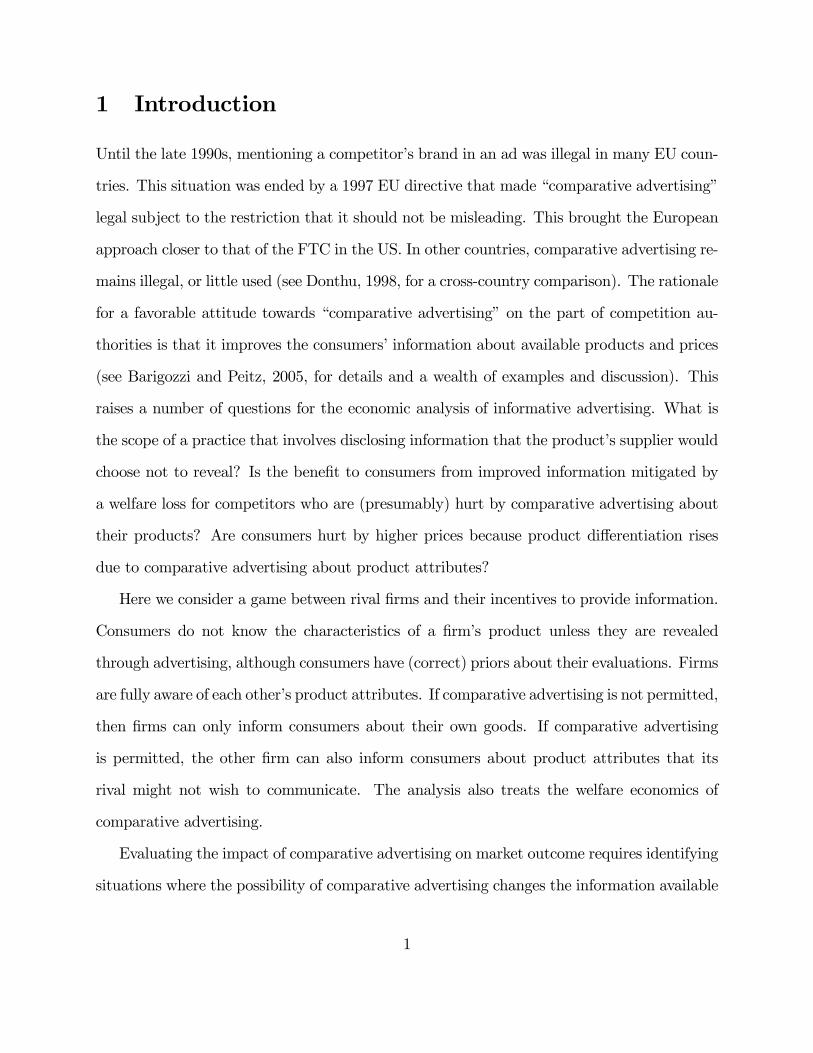
The following Figures have Q on the horizontal axis and profits on the vertical.

32.521.510.50

2.5

2

1.5

1

0.5

0

quality difference, Q

profit

quality difference, Q

profit

The upward-sloping lines are Firm 1’s profits for no information (magenta), full infor-

mation (green), and one-sided information (blue). While full information always dominates

24

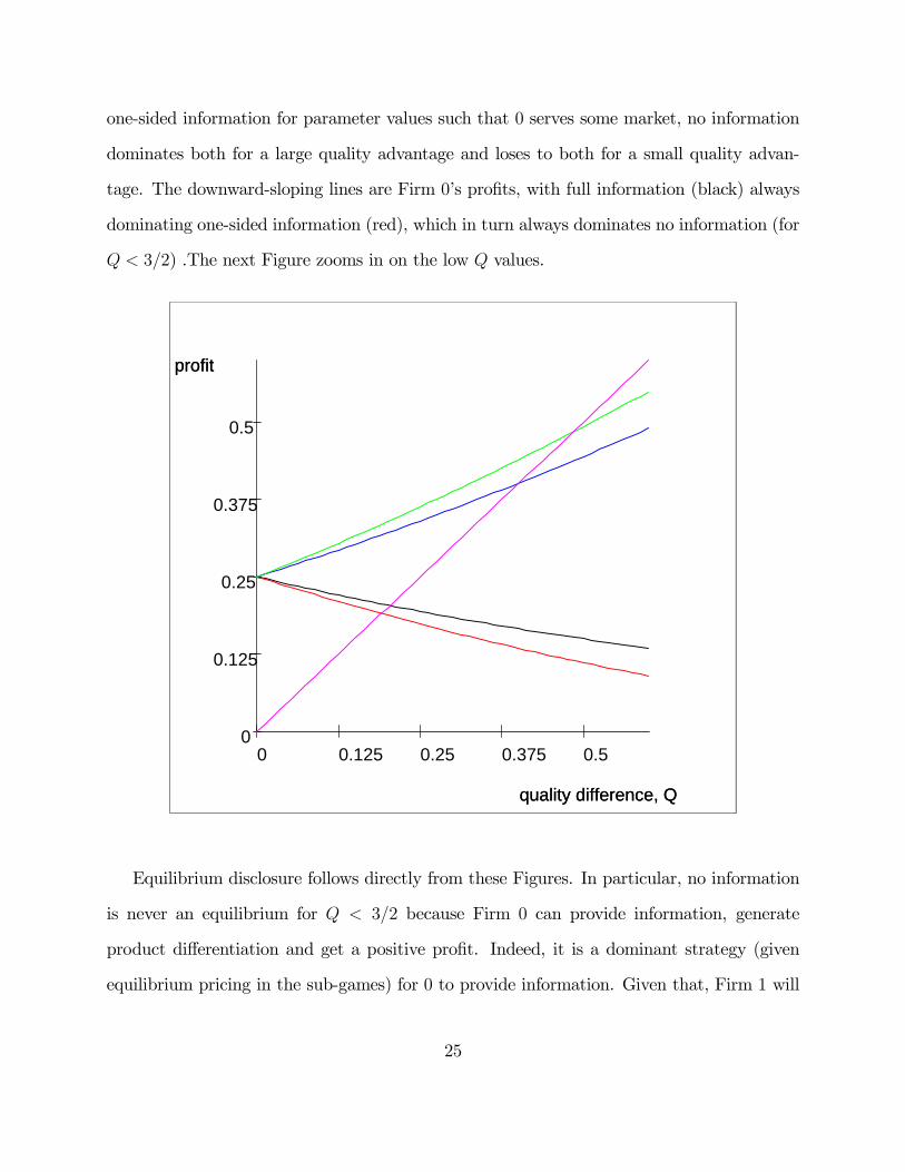
one-sided information for parameter values such that 0 serves some market, no information

dominates both for a large quality advantage and loses to both for a small quality advan-

tage. The downward-sloping lines are Firm 0’s profits, with full information (black) always

dominating one-sided information (red), which in turn always dominates no information (for

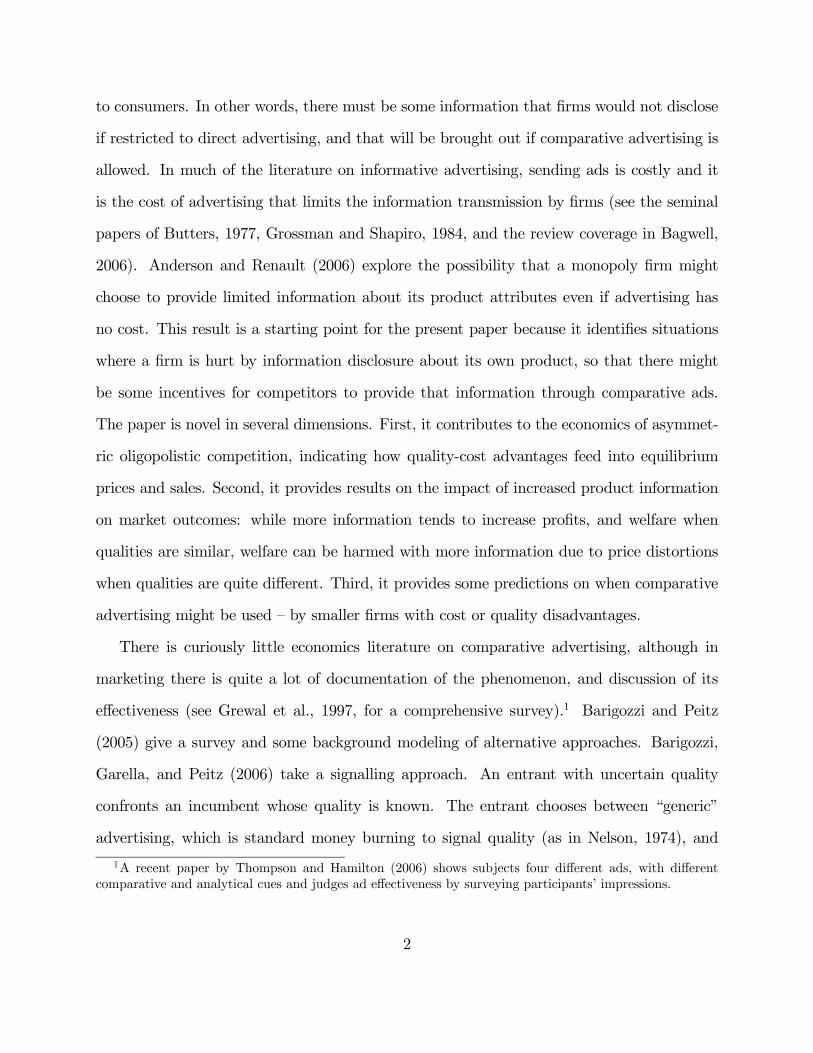
Q < 3/2) .The next Figure zooms in on the low Q values.

0.50.3750.250.1250

0.5

0.375

0.25

0.125

0

quality difference, Q

profit

quality difference, Q

profit

Equilibrium disclosure follows directly from these Figures. In particular, no information

is never an equilibrium for Q < 3/2 because Firm 0 can provide information, generate

product differentiation and get a positive profit. Indeed, it is a dominant strategy (given

equilibrium pricing in the sub-games) for 0 to provide information. Given that, Firm 1 will

25

always want to provide information itself. So here there is full revelation, and no role for

negative or comparative advertising insofar as any equilibrium still entails full revelation.11

Now consider Q > 3/2. The driver for the equilibrium is what happens to Firm 1’s profit

between full information and one-sided information.12 As per Lemma 9, this depends on

which side of Q the quality difference Q lies. For Q > Q (which exceeds 3/2), the only

equilibrium is for there to be no advertising if comparative advertising is not permissible (as

per Proposition 7): it is a dominant strategy (among the pricing sub-games) for 1 to NOT

reveal, and, in response, since 0 gets nothing either way, it does not reveal either (by the

tie-break rule that favors less information over more in case of indifference). Otherwise, the

only equilibrium is comparative advertising by Firm 0 (as per Proposition 8), which enables

it to survive.

For Q ∈h3/2, Q

i, equilibrium is driven by the twin properties that π1 < eπ1 < πzero1

and eπ0 > π0 = πzero0 (= 0). With comparative advertising debarred, one equilibrium has no

information provided, and another has both providing own match information. In the former

case, Firm 1 prefers no information to one-sided information and so does not advertise if

Firm 0 does not advertise, and Firm 0 will not advertise if Firm 1 does not. In the other

equilibrium, each firm prefers to advertise if the other advertises. Allowing now comparative

advertising, the latter is still an equilibrium, as is reciprocal negative advertising by the

same token. The former is not because Firm 0 would prefer comparative advertising, and

this comparative advertising is the other equilibrium.13 However, since Q > 1, comparative

11With comparative advertising allowed, there is an equilibrium with each providing information aboutmatches with its rival (“negative advertising”). There is another equilibrium with either of the firms providinga full comparison and the other doing nothing.12The one-sided information price, given the rival sets p0 = 0 and that Firm 1 serves the whole market,

must ensure that 1 gets on board the consumer who least likes it, which is r0 = −12 ; this means a price ofQ− 1/2 (since 1 delivers expected utility zero to all). Of course, this is less attractive than no information,whereby the price charged is Q (with no product differentiation, the keel is even).13Equilibrium strategies cannot involve Firm 1 giving a full comparison and 0 doing nothing, since 1 would

deviate to advertising nothing at all. Nor can they involve negative advertising by either alone: both preferfull information to one-sided information, which outcome they can get by either full comparative advertisingor indeed reciprocal neagative advertising.

26

advertising allows a weak firm to survive against the optimality rule.14

Finally, note that (using the price expressions in the Appendix) as Q becomes large, the

full information price for Firm 1 goes to Q − 1, whereas its one-sided information price isQ − 1

2. This shows that the full information price can be lower for the high quality firm.

Moreover, consumer surplus is higher under full information. Under one-sided information

all consumers buy from Firm 1, whereas under full information those who still buy from

Firm 1 pay a lower price and those choose to buy from Firm 0 are better off.

6 Discussion

It was assumed above that the good advertised is an experience good, and that qualities are

known to consumers beforehand. We first show that the results hold too when the good is

a search good as long as search costs are high enough. We then show that if qualities are

known to firms but not consumers, and firms can advertise quality information, then firms

will advertise qualities, so the basic set-up still holds.

6.1 A search good

Suppose that a consumer can observe the product’s attributes before making a purchase at

cost c > b. She must incur the visit cost c to buy from either firm, but the cost of the first

visit is irrelevant since the consumer must buy one of the two products in any case. We now

show that demands are exactly the same as with the experience good version of the model

(and so prices and equilibria are too). This we do by showing that the consumer always

buys from the first firm she visits so that the information she obtains when she gets there is

irrelevant.

Consider a consumer who, after observing prices and advertised information, decides to

14Comparative ads more generally might facilitate toe-hold entry for entrants to become larger later, andthis could be desirable in an extended context.

27

visit Firm i first. If information about product i was provided through advertising, then

the consumer has not learned anything from her first visit and she will clearly choose to

buy product i given that she initially chose to visit Firm i. Let us thus assume that ri was

unknown to her when she chose to visit Firm i. A first possibility is that she was informed

about her match with the other product when she made that choice. A standard sequential

search argument shows that she would then have chosen to incur search cost c to find out

about ri, if and only if her match with the competing product (rj, j 6= i) augmented by the

price difference pi − pj − c is strictly less than −c < −b.15 She will then choose to purchaseproduct i even if she finds out that ri = −b. Suppose finally that neither product was knownwhen the consumer decided on her first visit. Since she chose to visit Firm i first, we must

have pi ≤ pj. Then the search theoretic argument used above shows that, when she finds out

her match with product i, for any ri, she will not visit Firm j: since ri + pj − pi ≥ −b > −cit is not worth incurring search cost c to find out about rj.16 The ability of the consumer

to obtain product information which has not been advertised before buying therefore has no

impact on her choice of product since it would be too costly to use that information.

In an earlier version of this paper, we studied product information disclosure with a search

good. Assuming that only one of the two products is unknown, we found that the firm selling

the unknown product would disclose horizontal attributes if and only if its quality is below

the other product’s. Furthermore, a known product with low quality uses comparative adver-

tising (if allowed) to disclose information about an unknown high quality product.17 Hence

the predictions of the model with search (and only one product unknown), are qualitatively

similar to those derived in the present paper.

15Here pj + c is the price of the known product j.16Here the price of the known product is pi since the cost of visiting Firm i is already sunk. Furthermore,

the exact condition used here assumes that recalling Firm i’s offer after visiting Firm j has no cost.17These results hold as long as a pure strategy equilibrium exists, which is not necessarily the case for all

search cost values or quality differences.

28

6.2 Quality disclosure

Let us now consider the possibility that qualities as well as horizontal attributes are un-

known. A standard result in the literature due to Milgrom (1981) and Grossman (1981), is

that a monopoly firm that may disclose certifiable information about its product’s quality,

always discloses it in equilibrium. We now show that practically the same result holds for

our duopoly setting with horizontal differentiation as well as vertical (quality). Assume that

qualities for the two firms are independently drawn from the same distribution and that real-

izations are initially known only by firms. First note that no information disclosure is not an

equilibrium. In such an equilibrium, firms would engage in symmetric Bertrand competition

in the second stage and earn zero profit. It would be profitable for a firm to deviate and

disclose its horizontal attributes thus creating some product differentiation. Second, there is

no equilibrium where only the low quality firm discloses its quality. Recall that, independent

of what information is revealed about horizontal attributes, the high quality firm earns some

strictly positive profit that is strictly increasing in its quality. Suppose that for some given

low quality and horizontal attributes information disclosed, there is some non-zero subset of

high qualities that are not disclosed in equilibrium. The consumers form some conditional

expectation as to the quality of a firm that does not disclose so that any firm with a quality

above that conditional expectation is better off disclosing its quality.

Now consider the choice of a low quality firm. With no horizontal attributes disclosed

or if only one product’s attributes are disclosed and the quality difference is large enough,

it earns zero profits. Otherwise, its profit is strictly positive and strictly increasing in its

quality (Corollary 2). Whenever the latter situation arises, then an argument analogous to

that used for the high quality firm shows that the low quality is always revealed. The only

situation when the low quality firm cannot guarantee itself some strictly positive profit is

when the quality difference is very large and comparative advertising is not allowed. Then,

29

the low quality is not disclosed but consumers update their beliefs accordingly and anticipate

the low quality is very low relative to the high quality. The only information disclosed in

that case is the higher quality and the high quality firm serves the whole market.

To summarize, the only situation where the market outcome would not be fully identical

to that obtained while assuming that qualities are known is when the quality difference is

large and comparative advertising is not allowed. Then the low quality is not revealed but it

is anticipated by consumers to be much lower than the high quality. The market outcome is

qualitatively similar to that derived in previous sections where the quality difference should

be replaced by the difference between the high quality and some expected low quality.

7 Conclusions

Comparative advertising involves informing consumers of characteristics of rival products.

On the surface, the practice would appear socially beneficial (assuming of course that the

advertising is not misleading) and should lead to better informed choices. It has though

been pointed out that it may relax price competition (and lead to higher prices) because it

increases product differentiation. However, this is also true for direct advertising, so a useful

theory should also explain when it is used and not.

The theory proposed here does this by focussing on intrinsic quality differences in the

products sold. If these qualities are quite similar, firms have enough incentive to advertise

their own products and comparative advertising plays no role. This is true in a balanced

market with firms that have similar market shares. Only if product qualities or marginal

production costs are sufficiently different does the ability to use comparative advertising

come into play. If it is illegal, the dominant product can serve the market without needing

to advertise, and the minor product may be overwhelmed. If comparative advertising is legal

though, the minor product can improve its consumer base and survive by using advertising

30

that targets the dominant product and compares characteristics. Thus, the model predicts

that comparative advertising is used by weaker firms targeting market leaders. There is some

empirical support for the contention that the market leader does not engage in comparative

advertising, but those just behind it do. Tylenol has 25% of the market for over-the-counter

pain relievers, and does no comparative advertising regarding the other OTC medicines.

Advil, in second place with 15% of the market, spends over half (58%) of its advertising

budget on comparative ads, mainly about Tylenol.

The model also delivers a salutary message for comparative advertising. It enables weaker

firms to survive through an equilibrium pricing distortion whereby the stronger firm over-

prices its product. The dominant firm effectively parlays its quality advantage into both a

high mark-up and high sales. The paper shows that this distortion can be sufficiently acute

that it overwhelms the informational benefits of comparative advertising. However, some

caveats are worth drawing. First, even when total welfare falls, it may be that consumer

welfare rises since comparative advertising (full information) may be associated with lower

prices when quality (or cost) differences are large enough. Second, such lower prices might

entail a lower deadweight loss if the model were extended to allow for non-purchase options.

The modeling approach is based on truthful informative advertising of horizontal charac-

teristics with rational consumers. The approach was chosen to portray comparative adver-

tising in a favorable light by allowing the conveyance of more hard information. If consumers

were not rational (rationality is embodied in the model in the assumption that consumers

form correct expectations of mean valuations in the absence of information), they might be

manipulated by misleading advertising. The legal system may play an important role in

ensuring truthfulness in this context.

We have also assumed that firms only are able to convey full information or else none

at all. Partial information (in a monopoly context) is addressed in Anderson and Renault

(2006). The information portrayed here was assumed to be perfectly certifiable at no cost.

31

An approach to be investigated in future research is to allow for imperfect certification (see

Shin, 1994) and/or costly certification. Finally, advertising has been assumed to reach all

consumers costlessly. Introducing costly reach would be another worthwhile extension to the

model.

References

[1] Aluf, Yana, and Oz Shy (2001) Comparison advertising and competition. Mimeo, Uni-

versity of Haifa.

[2] Anderson, Simon P. and André de Palma (1988): Spatial Price Discrimination with

Heterogeneous Products. Review of Economic Studies, 55, 573 592.

[3] Anderson, Simon P. and André de Palma (2001): Product Diversity in Asymmetric

Oligopoly: Is the Quality of Consumer Goods Too Low? Journal of Industrial Eco-

nomics, 49, 113-135.

[4] Anderson, Simon P. and Renault, Régis (1999): Pricing, Product Diversity and Search

Costs: a Bertrand-Chamberlin-Diamond Model. RAND Journal of Economics, 30, 719-

735.

[5] Anderson, Simon P. and Renault, Régis (2000): Consumer Information and Firm Pric-

ing: Negative Externalities from Improved Information. International Economic Review,

31, 721-741.

[6] Anderson, Simon P. and Renault, Régis (2006): Advertising content. American Eco-

nomic Review, 96, 93-113.

[7] Bagwell, Kyle (2006): The Economic Analysis of Advertising. Mimeo, Columbia Uni-

versity.

32

[8] Barigozzi, Francesca, Paolo Garella, and Martin Peitz (2006): With a little help from

my enemy: comparative vs. generic advertising. Mimeo, University of Bologna.

[9] Barigozzi, Francesca andMartin Peitz (2005): Comparative advertising and competition

policy. Forthcoming in Recent Developments in Antitrust Analysis, edited by Jay Pil

Choi, MIT Press.

[10] Butters, Gerard R. (1977): Equilibrium Distributions of Sales and Advertising Prices.

Review of Economic Studies, 44, 465-491.

[11] Donthu, Naveen (1998): A cross-country investigation of and attitude toward compar-

ative advertising. Journal of Advertising, 27, 111-133.

[12] Grewal, Dhruv, Sukumar Kavanoor, Edward F. Fern, Carolyn Costley, and James

Barnes (1997): Comparative versus noncomparative advertising: a meta-analysis. Jour-

nal of Marketing, 61, 1-15.

[13] Grossman, Gene M. and Shapiro, Carl (1984): Informative Advertising and Differenti-

ated Products. Review of Economic Studies, 51, 63-81.

[14] Grossman, Sanford J. (1981): The informational role of warranties and private disclosure

about product quality. Journal of Law and Economics 24(3), 461-83.

[15] Liaukonyte, Jura (2006): Is comparative advertising an active ingredient in the market

for pain relief? Mimeo, University of Virginia.

[16] Meurer, Michael J., and Stahl, Dale O., II (1994): Informative Advertising and Product

Match. International Journal of Industrial Organization, 12, 1-19.

[17] Milgrom, Paul R. (1981): Good news, bad news: representation theorems and applica-

tions. Bell Journal of Economics, 12, 380-391.

33

[18] Nelson, Phillip J. (1974): Advertising as information. Journal of Political Economy. 82,

729-754.

[19] Shin, Hyun (1994): The Burden of Proof in a Game of Persuasion. Journal of Economic

Theory, 64, 253-263.

[20] Thompson, Debora Viana and Rebecca W. Hamilton (2006): The effects of informa-

tion processing mode on consumers’ responses to comparative advertising. Journal of

Consumer Research, 32, 530-540.

[21] Wolinsky, Asher (1986): True Monopolistic Competition as a Result of Imperfect Infor-

mation. Quarterly Journal of Economics, 101, 493-511.

34

Appendix

8 Proofs from Section 2

8.1 Lemma 1

Assume that Q ≥ 0. We first show that ∆ = Q or ∆ = 0 imply that Q = 0. Assume first

that ∆ = Q, so that p0 = p1 = p. Then, in order for Firm 0 not to wish to deviate, for any

real number δ ≥ −p we must have

p[1−D1(Q)] ≥ (p+ δ)[1−D1(Q+ δ)],

which is equivalent to

(p− δ)D1(Q+ δ) ≥ pD1(Q) + δ[1− 2D1(Q+ δ)].

If Q > 0, then for any δ ∈ (−Q, 0], D1(Q + δ) > 12and thus δ[1 − 2D1(Q + δ)] > 0. Then

Firm 1 could deviate from p to p− δ so as to earn a profit of (p− δ)D1(Q+ δ) which strictly

exceeds pD1(q). So we must have Q = 0 in order for ∆ to be equal to Q in equilibrium.

Now suppose that ∆ = 0 so that p0 = p1 −Q. Then, for any δ > 0 we must have

1

2(p1 −Q) ≥ (p1 −Q+ δ)[1−D1(δ)],

or, equivalently,

(p1 − δ)D1(δ) ≥ 12p1 + (δ − Q

2)[1− 2D1(δ)].

If Q > 0, since δ > 0 so that D1(δ) >12, for δ sufficiently small, the right hand side strictly

exceeds 12p1. Firm 1 would therefore be better off charging p1 − δ rather than p1. Thus in

order for ∆ to be zero in equilibrium we must have Q = 0.

We now show that in equilibrium 0 ≤ ∆ ≤ Q which, along with the results above, proves

the Lemma for Q ≥ 0. First, it is necessary that Firm i prefers pi to its rival’s price so that

p0[1−D1(∆)] ≥ p1[1−D1(Q)]

35

and

p1D1(∆) ≥ p0D1(Q).

Adding these two inequalities and rearranging yields

p0 − p1 ≥ (p0 − p1)[D1(Q) +D1(∆)]. (9)

Since Q ≥ 0, if p0 > p1, then D1(∆) > D1(Q) ≥ 12. Thus D1(Q) + D1(∆) > 1 which

contradicts inequality (9). So we must have p0 ≤ p1, or equivalently ∆ ≤ Q.

It must also be the case that Firm i prefers charging pi than a price that would set ∆ to

zero, so that

p0[1−D1(∆)] ≥ 12(p1 −Q)

and

p1D1(∆) ≥ 12(p0 +Q).

Adding these two inequalities yields

[1−D1(∆)]p0 +D1(∆)p1 ≥ 12(p0 + p1). (10)

We know from above that p1 ≥ p0. If p1 > p0, inequality (10) requires that D1(∆) ≥ 12and

therefore ∆ ≥ 0. If p1 = p0 then ∆ = Q ≥ 0. This completes the proof for Q ≥ 0.Similar arguments establish the result for Q ≤ 0. Q.E.D.

8.2 Lemma 2

If ∆ < ∆ or∆ > ∆u, then whichever firm has a demand of 1 could increase its price without

losing any demand and thus, increase it profit; this proves the first part of the Lemma.

We now show that differentiability at ∆k implies that ∆ = ∆k cannot be an equilibrium.

For instance for k = u, differentiability at ∆u implies that the left derivative of D1 at ∆u is

0 (since the right derivative is zero). Then Firm 1’s profit derivative is D1(∆u) = 1 > 0 so

that Firm 1 would deviate and increase its price. Similarly, if ∆ = ∆ , Firm 0 would wish

to increase its price from the candidate equilibrium. Q.E.D.

36

8.3 Proposition 1

The argument for existence is standard (see Caplin and Nalebuff, 1991).

Before going through the 3 cases it is useful to note that since D1 and D0 = 1−D1 are

strictly log-concave, g is strictly decreasing on [∆ ,∆u] and so the right-hand side of equation

(3) (the equation is Q = ∆− g (∆)) is strictly increasing on that same interval. This shows

that ∆ is uniquely defined in Case 1. Furthermore, because D0i

Di, i = 0, 1 is strictly increasing,

prices are uniquely determined by equation (1). It also shows that in this case ∆ must be

strictly increasing in Q. Implicit differentiation of (3) and Assumption 2 imply d∆dQ

< 1.

First consider case 3. If ∆ ≤ ∆ , then Firm 1 makes zero profit whereas, since Q > 0.

it could obtain a strictly positive profit by charging, for instance, a price p0 +Q > 0. Next

note that ∆u +1

D01(∆u)

is the right-hand side of (3) evaluated at ∆ = ∆u. Since Q is at

least as large and the right-hand side of (3) is strictly increasing on (∆ ,∆u), there is no ∆

in that interval that satisfies (3). Since an equilibrium exists and using Lemma 2, we must

have ∆ = ∆u. We also know from Lemma 2 that this case may arise only if D01(∆u) > 0 so

that Firm 0’s profit left derivative with respect to p0 is −p0D01(∆u) which would be negative

if p0 > 0 and thus Firm 0 would wish to decrease its price. Thus we have p0 = 0 and the

expression for p1 follows.

Case 2 may be treated with symmetric arguments.

Now consider case 1. We show that we may not have ∆ = ∆u and a symmetric argument

would show that we cannot have ∆ = ∆ . From Lemma 2, this suffices to complete the

proof. Hence suppose that ∆ = ∆u. As was shown above, we must then have p0 = 0. The

right derivative of Firm 1’s profit is given by 1 − p1D01(∆u) = 1 − (Q −∆u)D

01(∆u). Since

Q < D1(∆u) +1

D01(∆u)

the right derivative of profit strictly exceeds 0. Then Firm 1 could

increase its profit by increasing its price. Q.E.D.

37

8.4 Proposition 2

From symmetry of f , equality clearly holds if ∆ = 0. We now show that the inequality holds

strictly for ∆ > 0. Symmetry of f impliesZ b

−bF (r +∆)f(r)dr =

Z 0

−b[F (r +∆) + F (−r +∆)] f(r)dr,

and

F (∆) =

Z 0

−b2F (∆)f(r)dr.

Hence it suffices to establish that F (r + ∆) + F (−r + ∆) < 2F (∆) for all r < 0. This is

equivalent to

F (−r +∆)− F (∆) < F (∆)− F (r +∆)

or Z −r+∆

∆

f(s)ds <

Z ∆

r+∆

f(s)ds

Using appropriate changes of variables, this condition may be rewritten asZ −r

0

f(∆+ t)dt <

Z −r

0

f(∆− t)dt.

Since∆ > 0, quasi-concavity and symmetry of f around zero implies that f(∆+t) < f(∆−t),for all t ∈ (0,−r]. This ensures the proper inequality.Symmetric arguments establish reverse inequalities for ∆ < 0. Q.E.D.

8.5 Pricing expressions for the uniform density

We give a free-standing derivation of equilibrium prices for the uniform density f (x) = 1 for

x ∈ £−12, 12

¤, and zero otherwise.

8.6 One-sided information

Since D1(∆) = F (∆) in general, for the uniform density we have D1(∆) =12+ ∆ for

∆ ∈ £−12, 12

¤and D1(∆) is zero below the lower bound and one above the upper bound.

38

When within the bounds, D01 = −1, so we have a simple linear demand system.18

We can immediately determine the equilibrium prices for ∆ ∈ £−12, 12

¤as

p1 =1

2+∆ and p0 =

1

2−∆.

These prices depend only on net quality differences so we may apply Lemma 1.

Taking the difference of these two equations we can write out and solve for ∆ = Q/3.

Substituting back gives prices as

p0 =1

2− Q

3, and p1 =

1

2+

Q

3,

which therefore hold for the interior regime, with∆ = Q+p0−p1 = Q/3 (which is consistent

with Lemma 1): so that this regime applies when Q < 3/2 (recall Q > 0). Equilibrium profit

levels are given by these prices squared (as is standard for linear demands with unit slopes).

Otherwise, for Q ≥ 3/2, we have

p0 = 0 and p1 = Q− 12.

Here the quality-advantaged firm prices so as to just retain the individual retaining the

highest regard for Firm 0, which is the individual who has a match r0 = 1, which compares

to the mean value of 0 for Firm 1.19

8.7 Full information

For the uniform density, recalling that r1 ∈£−1

2, 12

¤, (6) becomes

eD1(∆) =

Z 1/2−∆

−1/2

µ1

2+ r1 +∆

¶dr1 +∆ =

1 + 2∆−∆2

2

18The "symmetric" version, with consumers knowing their valuations at both firms, does NOT give alinear demand system. This latter system is determined in the text below.19Equivalently, as per Lemma 3, if Firm 1 reveals its match information while Firm 0 does not, 1 must

price so that the consumer least enamoured of it (holding r1 = 0) nonetheless buys against an expected valueof 0 with Firm 0.

39

Notice that ∆ < 1 for both firms to have positive demands: for ∆ > 1, Firm 1’s demand

is eD1(∆) = 1, but, by Lemma 1, this is never relevant.20 Firm 0’s demand is 1− eD1(∆) or:

eD0(∆) =(1−∆)2

2

Since evaluations for the two products are i.i.d. we have eD1(0) =12, and all assumptions of

Lemma 5 are satisfied. Thus the firm with the higher quality will set a higher net quality

and thus garner a larger share of demand, even though it charges the higher price.21

We now find the equilibrium prices conditional on consumers knowing product specifica-

tions and qualities of both products (Perloff-Salop, uniform distribution, with asymmetric

qualities, effectively). Since eD0 (∆) =(1−∆)2

2, the first order condition for Firm 0 yields

p0 =(1−∆)

2;

we can immediately substitute in for ∆ = Q+ p0 − p1 to yield a linear reaction function

p0 =1−Q+ p1

3.

For Firm 1, we have the first order condition 1− (1−∆)22− p1 (1−∆) = 0.

Substituting in p0 =(1−∆)2, then 1− 2p20 − 2p0p1 = 0.

Solving out these equations for prices then gives the solutions as

p0 =ω +

p8 + ω2

8, and p1 =

−5ω + 3p8 + ω2

8,

where ω = 1−Q. Note that these prices are equal at ω = 1 (symmetry) to one half. They

also verify ∆ > 0, as desired.

20Demand is convex for ∆ < 0 (high prices for Firm 1) and concave for ∆ > 0 (low prices). The demandderivative is continuous on its support, and so there is no kink.21Any best reply price for Firm 1 must satisfy p1 ∈ [0, p0 + q1 − q0 − 1], where the upper bound is where

Firm 1’s demand disappears. Hence Firm 1’s profit is a continuous function that is defined over a compactset, and so has a maximum. Equilibrium existence follows from Caplin and Nalebuff (1991).

40