Compact HVDC ±320 kV lines proposed for the Nelson River...

Compact HVDC ±320 kV lines proposed for the Nelson River Bipole 3:

Consideration of the dimensions of the shield conductors, and initial review of the overall corona and field effects

Compiled by:

AC Britten, Pr Eng

2/21/2014

Mobile: +27-72-204-6086

Landline: +27-11-706-4542

Email: [email protected]

Compiled for:

Mr DA Woodford, CEO of the Electranix Corporation of Winnipeg, Canada

EXECUTIVE SUMMARY COMPACT AND CONVENTIONAL STRUCTURES:

The results of an initial study of the corona and field effects produced by the proposed compact ±320 kV

HVDC line carrying two symmetrical monopolar circuits are presented. The results are compared with those

produced by the conventional bipolar configuration being proposed for Bipole 3. The effects of unbalanced

supply voltages on the corona performance of the compact line are quantified. How the optimum diameter of

the shield conductor is determined is explained. It is concluded that the compact line offers acceptable corona

performance from both engineering and environmental considerations, and also better performance than

predicted for Bipole 3. It is pointed out that the contingent question of the susceptibility of the compact design

to anomalous flashovers is still unresolved; however, it is speculated that reducing the ion generation may help

mailto:[email protected]

REPORT NUMBER: ACB/1/14

Confidential

Revision: 1

Page: 2 of 28

Classification:

to mitigate this problem. Other aspects, such as those related to the lightning, switching and pollution

withstand levels, have not been evaluated at this stage.

CONTENTS

Page

1. INTRODUCTION ...................................................................................................................................................... 4

2. TECHNICAL PARAMETERS, APPROACH AND METHODOLOGY ..................................................................... 4

3. RESULTS AND ANALYSIS ..................................................................................................................................... 5

3.1 COMPACT STRUCTURE: CONDUCTOR SURFACE GRADIENTS (SHIELD AND POLE CONDUCTORS)................................................................................................................................................. 5

3.2 COMPACT AND CONVENTIONAL STRUCTURES: AUDIBLE NOISE ........................................................... 8 3.3 COMPACT AND CONVENTIONAL STRUCTURES: RADIO INTERFERENCE 10

3.4 COMPACT AND CONVENTIONAL STRUCTURES: ELECTRIC FIELDS 11

4. CONCLUDING REMARKS .................................................................................................................................... 14

5. REFERENCES ....................................................................................................................................................... 15

6. APPENDICES ........................................................................................................................................................ 16

6.1 APPENDIX A1: EXAMPLE OF THE DATA SHEET USED BY THE TLW PROGRAMME ............................. 16 6.2 APPENDIX A2: RAW DATA FOR THE COMPACT LINE STUDIES .............................................................. 20


Confidential

Revision: 1

Page: 4 of 28

Classification:

1. INTRODUCTION

In January 2014 the author was requested by Mr DA Woodford, CEO of Electranix Corporation, to

investigate the sizing and position, from a corona and electric field effects point of view, of the two

underhanging shield conductors on the compact ±320 kV HVDC structure shown in Figure 1. It is

understood that this structure is being considered for possible implementation in the Nelson River Bipole

3 Expansion Programme, so as to lessen the environmental impact of the scheme [1,2].

Also included in this report are the results of initial comparisons between the corona and field parameters

of the likely conventional ±500 kV tower, proposed for use in Bipole 3, and the ±320 kV compact

structure. (See Figures 1 and 2.)

2. TECHNICAL PARAMETERS, APPROACH AND METHODOLOGY

The author was requested to estimate and quantify the following parameters at ±320 kV for the compact

tower geometry (Figure 1) and each of two pole conductor bundles, namely, 1x4.475 cm and 2x3.038

cm, with a spacing of 40-45 cm:

Variation of the conductor surface gradients on the pole and shield conductors as a function of

the diameter of the shield conductor.

Audible noise lateral profiles at midspan.

Audible noise and electric field levels at the 30 m lateral midspan positions, where the tower

centre line is the reference position.

Electric field lateral profile, with and without space charge, at midspan.

The author will also offer some comment on the limits of audible noise and electric fields for

consideration by Electranix. The author also decided to include a comparison between the radio

interference characteristics of the compact and conventional structures.

The predictions have been done means of the EPRI TLW 3.0 Programme. The key results are given

mainly in the form of graphs in the body of the report, and relevant raw data in the appendices.

The elements of the compact ±320 kV compact structure are shown in Figure 1, as already noted. The

conventional ±500 kV structure, which is understood to be the preferred option for Bipole 3, is shown in

Figure 2.

It has been assumed that operation of the system as two ungrounded VSC-fed, balanced monopoles will

imply that ideally the pole-to-ground voltages will be equal in magnitude, but opposite in polarity [3,4,5].

This means that the pole-to-pole voltage used in the studies was 640 kV, with the two pole voltages

being +320 kV and -320 kV with respect to earth and the neutral point of the source. As the author

understands the possible influence of unbalanced pole-to-ground resistive loading, the pole-to-pole

voltage will still be 640 kV, but with the so called common mode voltages being higher on one pole than

on the other; their sum will still be 640 kV [1,2]. The author has, for the purposes of these studies,

assumed voltage unbalance levels of 0 to 25 %.


Confidential

Revision: 1

Page: 5 of 28

Classification:

Figure 1: Dimensions of the proposed compact HVDC structure [1,2]

Figure 2: Dimensions of the tower being proposed for the Nelson River Bipole 3 [1]

3. RESULTS AND ANALYSIS

The results of the studies are summarised below.

COMPACT STRUCTURE: conductor surface gradients (Shield and pole conductors)

All the studies done in this report assume and use “phasing” which requires the same polarity voltages to

be applied on the same side of the tower. This minimises the conductor surface gradient on the pole

conductor bundle. (See Table 1) It is also shown that the above form of phasing does not minimise the


Confidential

Revision: 1

Page: 6 of 28

Classification:

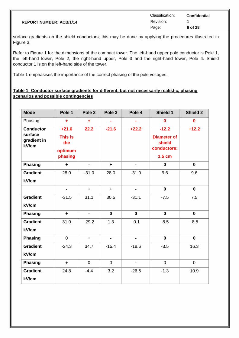
surface gradients on the shield conductors; this may be done by applying the procedures illustrated in

Figure 3.

Refer to Figure 1 for the dimensions of the compact tower. The left-hand upper pole conductor is Pole 1,

the left-hand lower, Pole 2, the right-hand upper, Pole 3 and the right-hand lower, Pole 4. Shield

conductor 1 is on the left-hand side of the tower.

Table 1 emphasises the importance of the correct phasing of the pole voltages.

Table 1: Conductor surface gradients for different, but not necessarily realistic, phasing

scenarios and possible contingencies

Mode Pole 1 Pole 2 Pole 3 Pole 4 Shield 1 Shield 2

Phasing + + - - 0 0

Conductor

surface

gradient in

kV/cm

+21.6

This is

the

optimum

phasing

22.2 -21.6 +22.2 -12.2

Diameter of

shield

conductors:

1.5 cm

+12.2

Phasing + - + - 0 0

Gradient

kV/cm

28.0 -31.0 28.0 -31.0 9.6 9.6

- + + - 0 0

Gradient

kV/cm

-31.5 31.1 30.5 -31.1 -7.5 7.5

Phasing + - 0 0 0 0

Gradient

kV/cm

31.0 -29.2 1.3 -0.1 -8.5 -8.5

Phasing 0 + - - 0 0

Gradient

kV/cm

-24.3 34.7 -15.4 -18.6 -3.5 16.3

Phasing + 0 0 - 0 0

Gradient

kV/cm

24.8 -4.4 3.2 -26.6 -1.3 10.9


Confidential

Revision: 1

Page: 7 of 28

Classification:

It can be clearly seen that the +-+- phasing would cause unacceptably high conductor surface gradients

on the pole conductors. This would probably increase the risk of anomalous flashovers, in the opinion of

the author.

.

Figure 3: Surface gradients on the shield conductors, for two different conductor bundle sizes

The data in figure 3 suggests that the diameter of the shield conductor should be at least 1.5 cm; this is

to limit the gradient to about 12 kV/cm, and is a value derived from the author’s experience on the

Cahora Bassa scheme [3].

Figure 3 also demonstrates that the larger the effective coupling area of the pole conductor bundle, the

higher will be the surface gradient on the shield conductor. This helps to improve one’s insight into

coupling mechanisms on a dc line.

Figure 4: Same as Figure 3, but shows more detail

5

10

15

20

25

30

35

0.5 0.75 1 1.25 1.5 1.75 2 2.25 2.5

Co

nd

uct

or

surf

ace

gar

die

nt

in k

V/c

m

Diameter of shield conductor in cm

Variation of surface gradient on shield conductors with their diameter for the balanced voltage case

Surface gradient onSHIELD conductor,2x3.04 cm case

Surface gradient onSHIELD conductor,1x4.43 cm case

SHIELD conductorsurface gradient: limitof 12 kV/cm suggested

-30

-20

-10

0

10

20

30

0.5 0.75 1 1.25 1.5 1.75 2 2.25 2.5

Co

nd

uct

or

surf

ace

gra

die

nt

in k

V/c

m

Diameter of shield conductor in cm

COMPACT STRUCTURE: variation of the SHIELD and POLE conductor surface gradients with

diameter of the shield conductor

Negative conductorsurface gradient onSHIELD conductor

Positive conductorsurface gradient onSHIELD conductor

Positive conductorsurface gradient onPOLE conductor


Confidential

Revision: 1

Page: 8 of 28

Classification:

In Figure 4, the point is made that the surface gradient on the pole conductors is insensitive to changes

in the diameter of the shield conductor. This is not the case when voltage unbalance is present, as can

be deduced from Figure 5.

Figure 5: Influence of voltage unbalance on shield and pole conductor surface gradients

COMPACT AND CONVENTIONAL STRUCTURES: Audible Noise

Audible noise levels are expressed here in terms of Ldn which is essentially a 24-hour weighted average

sound pressure level [6,7,8]. The weighting refers not only to the well-known frequency or A weighting,

but also weighting which depends on the time of day. What this means is that between 21h00 and 07h00,

10 dB is automatically added to the averaged noise levels measured during this period. The result is that

the 24-hour weighted level is higher than it would have been without weighting. Thus, to meet a given

limit of noise from a dc power line in this case, it would be necessary for the designer to reduce the noise

by an amount equal at least to the difference between the average weighted and unweighted levels. The

unweighted level is often referred to as the equivalent A-weighted level or Laq..

Leq quantifies the energy in a sound pressure signal; mathematically, it is given by the average value in

a time period T of the sum of the squares of the sound pressures.

The measure of power line noise is nowadays more and more being expressed in terms of Ldn. This

metric lends itself to the measurement of DC line noise, because positive polarity DC audible noise is

highest in fair-weather, and drops in rain conditions, unlike audible noise from AC lines, which increases

in foul-weather. This makes the application of the Ldn concept and limits more straight-forward and less

ambiguous for the designer to meet than in the case of AC. Another important point is that Ldn is widely

used in international and national noise regulations.

Another point to note is that the annual statistical spread of the values of Leq, typically the 24-hour

values, depend on the climate in a given area. Techniques have been developed for deriving the

resultant value of Ldn from a large number of Leq values [9].

The above text helps to explain why the author has concentrated on the Ldn metric for expressing noise,

from DC lines in particular.

-40

-20

0

20

40

0 5 10 15 20 25

Co

nd

uct

or

surf

ace

gra

die

nt

in

kV/c

m

Voltage unbalance in %

COMPACT STRUCTURE : variation of pole and shield conductor surface gradients with voltage

unbalance

Positive pole conductor

Positive shieldconductor

Negative shieldconductor

Negative pole


Confidential

Revision: 1

Page: 9 of 28

Classification:

Figure 6: Audible noise, expressed in Ldn, from the compact and conventional DC lines

If a limit of Ldn = 50 dBA at the edge of the right of way were to be applied to the data in Figure 6, it can

be seen that the two lower curves comply easily. The curve for the single conductor bundle compact line

(where the left-hand portion is generated by positive corona) just complies. It can be deduced that the

compact design does not constitute an audible noise problem under conditions of balanced supply

voltage. The data in Figure 7 (for the one conductor bundle) shows, however, that a sustained positive

voltage unbalance of a few percent, will cause the 50 dBA limit to be exceeded.

Audible noise will to some extent be a constraining factor in the application of the compact design, if

voltage unbalance does indeed occur. (Note that the conventional design does of course not experience

voltage unbalance.)

Figure 7: Variation of the audible noise levels at the ±30 m positions, with voltage unbalance

3.3 COMPACT AND CONVENTIONAL STRUCTURES: Radio interference

30

40

50

60

-50 -40 -30 -20 -10 0 10 20 30 40 50

Au

dib

le n

ois

e L

dn

in d

BA

Lateral distance from c/l of line in m

Comparison between the audible noise levels for the compact and conventional

lines

Conventional Bipole3 design

Compact, 2x3.04 cmconductor

compact, 1x4.44 cmconductor

30

35

40

45

50

55

60

0 5 10 15 20 25

Au

dib

le n

ois

e le

vel L

dn

in d

BA


AUDIBLE NOISE Ldn AS A FUNCTION OF VOLTAGE UNBALANCE

Increasing positivevoltage

Decreasing positivevoltage


Confidential

Revision: 1

Page: 10 of 28

Classification:

Figure 8: radio interference profiles in heavy rain conditions

The comparison between the radio noise profiles for the compact HVDC and the Bipole 3 designs shows

(Figure 8) that the compact line out-performs the conventional design by a considerable margin. If power

line carrier were to be used, the noise performance of the compact line, being superior to that of the

conventional design, would make the power line carrier system easier to engineer.

3.4 COMPACT AND CONVENTIONAL STRUCTURES: Electric Fields

The author has been informed that the main concern as regards electric fields is the question of the

degree to which such fields can be perceived by persons, become annoying or become dangerous.

These aspects have been studied for both the compact line and the conventional tower designs. Unlike

the case for audible noise, the important limit to be complied with is the maximum field, and not just the

field at the edge of the right of way.

The response of humans to electric fields varies, on average, as shown in the Table 2 below.

Table 2: Subjective assessments of the electrostatic and space charge – enhanced electric fields

[7,8,9,10]

Typical Voltage kV Electric Field kV/m

Result Reaction

+400 +22 Very slight sensation on scalp.

Aware of field

+500 +27 Hair stimulation, slight feeling on ears and hair.

Moderate nuisance

+600 +32 Strong tingling sensation on scalp.

Disturbing nuisance

+750 +40 Sensation on face and legs.

Very disturbing to painful

20

30

40

50

60

70

-50 -40 -30 -20 -10 0 10 20 30 40 50

Rad

io in

terf

ere

nce

dB

(1

µV

/m)

@ 0

.5

Mh

z

midspan lateral position m

Variation of radio noise in heavy rain midspan lateral profiles for average conductor

heights

Compact design

Bipole 3


Confidential

Revision: 1

Page: 11 of 28

Classification:

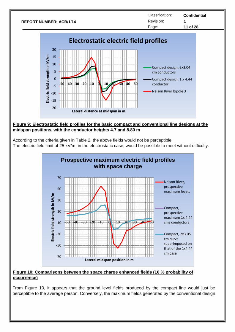
Figure 9: Electrostatic field profiles for the basic compact and conventional line designs at the

midspan positions, with the conductor heights 4.7 and 8.80 m

According to the criteria given in Table 2, the above fields would not be perceptible.

The electric field limit of 25 kV/m, in the electrostatic case, would be possible to meet without difficulty.

Figure 10: Comparisons between the space charge enhanced fields (10 % probability of

occurrence)

From Figure 10, it appears that the ground level fields produced by the compact line would just be

perceptible to the average person. Conversely, the maximum fields generated by the conventional design

-20

-15

-10

-5

0

5

10

15

20

-50 -40 -30 -20 -10 0 10 20 30 40 50

Ele

ctri

c fi

eld

str

en

gth

in k

V/m

Lateral distance at midspan in m

Electrostatic electric field profiles

Compact design, 2x3.04cm conductors

Compact design, 1 x 4.44conductor

Nelson River bipole 3

-70

-50

-30

-10

10

30

50

70

-50 -40 -30 -20 -10 0 10 20 30 40 50

Ele

ctri

c fi

eld

str

en

gth

in k

V/m

Lateral midspan position in m

Prospective maximum electric field profiles with space charge

Nelson River,prospectivemaximum levels

Compact,prospectivemaximum 1x 4.44cms conductors

Compact, 2x3.05cm curvesuperimposed onthat of the 1x4.44cm case


Confidential

Revision: 1

Page: 12 of 28

Classification:

will be “very disturbing” to “painful”. This could be an important point in favour of the use of the compact

structure.

Figure 11: Maximum ground level electric field in ROW, for the compact design, with voltage

unbalance the variable

Figure 12: Ion current density profiles for the two tower configurations, for rated voltage

-40

-30

-20

-10

0

10

20

30

40

0 5 10 15 20 25

Ele

ctri

c fi

eld

str

en

gth

in k

V/m


COMPACT STRUCTURE: Variation of maximum electric field with voltage unbalance

Positive electric field

negative electric field

-300

-200

-100

0

100

200

300

-50 -40 -30 -20 -10 0 10 20 30 40 50

ion

cu

rre

nt

de

nsi

ty in

nA

/m2

Lateral midspan position in m

Ion current density profiles at rated balanced voltage

Compact line, ioncurrent density innA/m2

Bipole 3, ion currentdensity, nA/m2


Confidential

Revision: 1

Page: 13 of 28

Classification:

Figure 13 Ion concentrations for 25% unbalance, for the compact and (balanced) conventional

lines

The results contained in Figures 12 and 13 show, or suggest that, the ion concentrations under the

positive and negative poles of the compact will be quasi–balanced.

Figure 14: maximum ion concentrations which have a 1% probability of being exceeded in a cold North American climate

It is observed in Figure 13 that the peak ion concentrations near the conventional structure for Bipole 3 are about twice those applicable to the compact designs. Figure 14 shows the profile for the existing Bipole 2 line geometry; it is clear that the peak ion concentrations under these lines, in transverse wind conditions, are substantially higher than the values predicted for Bipole 3. The high ion concentration

-250000

-200000

-150000

-100000

-50000

0

50000

100000

150000

200000

250000

-50 -40 -30 -20 -10 0 10 20 30 40 50

Ion

co

nce

ntr

atio

n in

ion

s/cm

3

Lateral midspan position m

Ion density profiles for bipole 3 and compact design with voltage unbalance

Bipole 3

Compact line, 25 % voltageunbalance

Compact line, balancedvoltages

-400000

-300000

-200000

-100000

0

100000

200000

300000

400000

-50 -40 -30 -20 -10 0 10 20 30 40 50

Ion

co

nce

ntr

atio

n in

ion

s/cm

3

Lateral midspan position m

Ion concentration profiles for compact line and Bipoles 2 and 3

Existing Bipole 2

Proposed Bipole 3

Compact line


Confidential

Revision: 1

Page: 14 of 28

Classification:

provides a clue about where to look for factors which could contribute to the high incidence of anomalous line faults.

The author has looked into this aspect and has found that the ratio of the pole-to-pole spacing to the minimum conductor height is unusually high in the case of the original Nelson River lines; this fact combined with the high conductor surface gradient on the these lines, could provide a fruitful and useful direction for further investigation.

As regards the compact design, the author’s assessment at this stage is that such lines will not suffer from anomalous negative polarity flashovers.

4. CONCLUDING REMARKS

What has this preliminary study revealed about the viability of a heavily compacted ±320 kV HVDC line

from corona and field effect points of view?

Can such a line be engineered to be compatible with the environment, and yet withstand some elements

the environment?

To what extent will the compact design be affected by the yet unexplained factors which cause

anomalous flashovers of the Nelson River HVDC lines?

How does the corona performance of the compact line compare with that of conventional HVDC bipolar

lines?

These are just a few of the questions which this study has looked into; it is felt that some progress has

been made in providing answers to them.

The author contends that the studies have clearly revealed the following findings:

The surface gradients on the pole and shield conductors can be kept economically to values low enough to prevent the generation of excessive space charge.

The author speculates that voltage unbalance may occur, but that its extent is still unknown.

In the event of unbalance occurring, special attention may have to be given to the suppression of abnormal corona; however, this is seen as “doable”, an aspect that, can be engineered “not to be a problem”.

Compared with conventional ±500 kV HVDC lines, the compact design gives better corona performance. This is an encouraging finding, especially in relation to the much lower ion generation by the compact line design.

The lower conductor surface gradients and reduced ion generation suggest that anomalous flashovers on the compact lines should not be a problem.

The radio interference studies done on the compact and conventional designs show that the former design meets acceptable limits of noise.

Overall, the corona and field effect assessments show that the compact design (as given in Figure 1) is

viable from a corona and field effects point of view, provided the voltage unbalance can be kept to below

25 %.


Confidential

Revision: 1

Page: 15 of 28

Classification:

5. REFERENCES

1. DA Woodford, Compact high voltage electric power transmission. Electranix Corporation, Winnipeg, Canada, January 2014.

2. DM Larruskain et al, VSC-HVDC configurations for converting AC distribution lines into DC lines. Electrical Power and Energy Systems 54 (2014) pp 589-597.

3. AC Britten et al, Extraneous electromagnetic noise in the Cahora Bassa power line carrier system, Proceedings of 2006 HVDC Congress, University of KwaZulu Natal (Westville Campus), Durban, South Africa, 14-16 July 2006.

4. MMC Merlin et al, A new multi-level VSC converter with DC fault blocking capability. IET International Conference on AC/DC transmission, 2010.

5. GP Adam et al, Network fault tolerant Voltage Source Converters for high voltage applications. Ibid [4].

6. P Sarma Maruvada, Corona performance of high voltage transmission lines. Research Studies Press LTD, UK, 2000.

7. HVDC Transmission Line reference Book, EPRI TR 102764, September, 1993.

8. Transmission line reference book: HVDC to ±600 kV. EPRI Project RP 104, 1977.

9. EPRI AC Transmission line handbook: 200 kV and above, third edition, 2005.

10. Bipole 3 DC EMF Brochure, Manitoba Hydro, October 2009.


Confidential

Revision: 1

Page: 16 of 28

Classification:

6. APPENDICES

APPENDIX A1: Example of the data output sheet generated by the TLW programme

COMPACT STRUCTURES:

Limited example of the printout as it relates to the calculation of the conductor surface gradient in a particular case.

Results of AC/DCLINE program CORONA (EPRI/HVTRC 7-93) for:

-------------------------------------------------------------

SURFACE GRADIENTS at AVERAGE LINE HEIGHT

CORONA LOSS

AUDIBLE NOISE

Configuration file name: C:\TLW30\ACDCLINE\DATA\ACCASE1

Date: 3/ 7/2014 Time: 13: 3

CASE1 compact dc with single conductor

**************************************************************************

* BUNDLE INFORMATION *

**************************************************************************

| | | VOLTAGE | CURRENT | # | BUNDLE COORDINATES | |

|BNDL|CIRC|VOLTAGE|ANGLE| LOAD |ANGLE| OF | X | Y | SAG | PH |

| # | # | (kV) |(DEG)| (A) |(DEG)|COND| (m) | (m) | (m) | |

**************************************************************************

| 1 | 1 | 320.0| 0.| 1000.| 0.| 1 | -3.65| 11.70| .00| + | POSITIVE POLE

| 2 | 1 | 320.0| 0.| 1000.| 0.| 1 | -3.65| 8.00| .00| + | POSITIVE POLE

| 3 | 1 | -320.0| 0.| 1000.| 0.| 1 | 3.65| 11.70| .00| - NEGATIVE POLE

| 4 | 1 | -320.0| 0.| 1000.| 0.| 1 | 3.65| 8.00| .00| - NEGATIVE POLE |

| 5 | 1 | . 0| 0.| 0.| 0.| 1 | -3.65| 4.70| .00| GND | SHIELD CONDUCTOR

| 6 | 1 | .0| 0.| 0.| 0.| 1 | 3.65| 4.70| .00| GND | SHIELD CONDUCTOR

**************************************************************************

* MINIMUM GROUND CLEARANCE = 4.70 meter *

* SOIL RESISTIVITY = 100 ohm meter *

* ALTITUDE ABOVE SEA LEVEL = 0 meter


Confidential

Revision: 1

Page: 17 of 28

Classification:

*************************************************************************

*****************************************************************************

* SUBCONDUCTOR INFORMATION - REGULAR BUNDLES *

*****************************************************************************

|BNDL | CONDUCTOR | DIAMETER | SPACING | DC RESIST | AC RESIST | AC REACT |

| # | NAME | (cm) | (cm) | (ohm/km) | (ohm/km) | (ohm/km) |

*****************************************************************************

| 1 |unnamed | 4.440 | .000

2 |unnamed | 4.440 | .000 |

3 |unnamed | 4.440 | .000 |

| 4 |unnamed | 4.440 | .000 |

| 5 |unnamed | 1.500 | .000 |

| 6 |unnamed | 1.500 | . 000 |

****************************************************************************

Results of AC/DCLINE program CORONA (EPRI/HVTRC 7-93) for:

-------------------------------------------------------------

SURFACE GRADIENTS at AVERAGE LINE HEIGHT

CORONA LOSS

AUDIBLE NOISE

Configuration file name: C:\TLW30\ACDCLINE\DATA\ACCASE1

Date: 3/ 7/2014 Time: 13: 3

CASE1 compact dc with single conductor

**************************************************************************

* BUNDLE INFORMATION *

**************************************************************************

| | | VOLTAGE | CURRENT | # | BUNDLE COORDINATES | |

|BNDL|CIRC|VOLTAGE|ANGLE| LOAD |ANGLE| OF | X | Y | SAG | PH |

| # | # | (kV) |(DEG)| (A) |(DEG)|COND| (m) | (m) | (m) | |

**************************************************************************


Confidential

Revision: 1

Page: 18 of 28

Classification:

| 1 | 1 | 320.0| 0.| 1000.| 0.| 1 | -3.65| 11.70| .00| + |

| 2 | 1 | 320.0| 0.| 1000.| 0.| 1 | -3.65| 8.00| .00| + |

| 3 | 1 | -320.0| 0.| 1000.| 0.| 1 | 3.65| 11.70| .00| - |

| 4 | 1 | -320.0| 0.| 1000.| 0.| 1 | 3.65| 8.00| .00| - |

| 5 | 1 | .0| 0.| 0.| 0.| 1 | -3.65| 4.70| .00| GND |

| 6 | 1 | .0| 0.| 0.| 0.| 1 | 3.65| 4.70| .00| GND |

**************************************************************************

* MINIMUM GROUND CLEARANCE = 4.70 meter *

* POWER SYSTEM FREQUENCY = 60. Hz *

* SOIL RESISTIVITY = 100. ohm meter *

**************************************************************************

*****************************************************************************

* SUBCONDUCTOR INFORMATION - REGULAR BUNDLES *

*****************************************************************************

|BNDL | CONDUCTOR | DIAMETER | SPACING | DC RESIST | AC RESIST | AC REACT |

| # | NAME | (cm) | (cm) | (ohm/km) | (ohm/km) | (ohm/km) |

*****************************************************************************

| 1 |DRAKE | 4.440 | .000 | .0720 | .0730 | .2480 |

| 2 |DRAKE | 4.440 | .000 | .0720 | .0730 | .2480 |

| 3 |DRAKE | 4.440 | .000 | .0720 | .0730 | .2480 |

| 4 |DRAKE | 4.440 | .000 | .0720 | .0730 | .2480 |

| 5 |DRAKE | 1.500 | .000 | .0720 | .0730 | .2480 |

| 6 |DRAKE | 1.500 | .000 | .0720 | .0730 | .2480 |

*****************************************************************************


Confidential

Revision: 1

Page: 19 of 28

Classification:

* * * MAXIMUM SURFACE GRADIENT (kV/cm) * * * ************************************ BNDL Type DC PEAK(+) PEAK(-) ------ --------- ------ ------- ------- 1 DC 22.34 22.34 22.34 2 DC 22.88 22.88 22.88 3 DC -22.34 -22.34 -22.34 4 DC -22.88 -22.88 -22.88 5 Ground Wire -10.35 -10.35 -10.35 6 Ground Wire 10.35 10.35 10.35


Confidential

Revision: 1

Page: 20 of 28

Classification:

APPENDIX A2: RAW DATA FOR THE COMPACT LINE STUDIES

Diameter of the shield conductor (Case 1: 1x4.44 cm pole conductor bundle)

Diameter

of

SHIELD

WIRE

(cm)

Conductor

surface

gradient on

SHIELD

WIRE

kV/cm, E5

Conductor

surface

gradient on

SHIELD WIRE

kV/cm, E6

Conductor

surface gradient

on Pos POLE

kV/cm

Conductor

surface gradient

on Neg POLE,

kV/cm

0.50 -26.58 +26.58 +22.32 -22.32

0.75 -18.71 +18.71 +22.33 -22.33

1.00 -14.62 +14.62 +22.33 -22.33

1.25 -12.08 +12.08 +22.33 -22.33

1.50 -10.25 +10.25 +22.34 -22.34

1.75 -9.08 +9.08 +22.34 -22.34

2.00 -8.12 +8.12 +22.34 -22.34

2.25 -7.35 +7.35 +22.35 -22.35

2.50 -6.75 +6.75 +22.35 -22.35

CASE 2: 2x3.038 cm

Diameter

of

SHIELD

WIRE

(cm)

Conductor

surface

gradient on

SHIELD

WIRE

kV/cm

Conductor

surface

gradient on

SHIELD WIRE

kV/cm

Conductor

surface gradient

on Pos POLE

kV/cm

Conductor

surface gradient

on Neg POLE,

kV/cm

0.50 -31.34 +31.34 +21.56 -21.56

0.75 -22.07 +22.07 +21.57 -21.57

1.00 -17.24 +17.24 +21.57 -21.57

1.25 -15.34 +15.34 +22.33 -22.33

1.50 -12.90 +12.90 +22.21 -22.21

1.75 -11.11 +11.11 +22.34 -22.34

2.00 -10.13 +10.13 +22.34 -22.34

2.25 -9.18 +9.18 +22.35 -22.35

2.50 -8.41 +8.41 +22.35 -22.35


Confidential

Revision: 1

Page: 21 of 28

Classification:

AUDIBLE NOISE

Audible noise case 1: 1x4.43 cm; lateral profile at midspan

Lateral

Distance

m

L50 FAIR

dBA

L5 RAIN

dBA

L50 RAIN

dBA

Leq (24)

dBA

Ldn

dBA

-50 38.9 32.9 32.9 38.9 45.2

-45 39.5 33.5 33.5 39.5 45.7

-40 40.1 34.1 34.1 40.1 46.4

-35 40.9 34.8 34.8 40.8 47.1

-30 41.7 35.6 35.6 41.6 47.9

-25 42.6 36.5 36.5 42.5 48.8

-20 43.6 37.6 37.6 43.6 49.9

-15 44.9 38.9 38.9 44.9 51.2

-10 46.4 40.2 40.2 46.2 52.7

-5 47.7 41.7 41.7 47.7 53.9

0 47.2 41.2 41.2 47.2 53.5

5 45,7 39.7 39.7 45.7 52.0

10 44.3 38.3 38.3 44.3 50.5

15 43.1 37.1 37.1 43.1 49.4

20 42.5 36.1 36.1 42.1 48.4

25 41.3 35.2 35.2 41.2 47.5

30 40.5 34.5 34.5 0.5 46.7

35 39.8 33.8 33.8 39.8 46.1

40 39.2 33.2 33.2 39.2 45.5

45 38.7 32.7 32.7 38.7 44.9

50 38.2 32.2 32.2 38.1 44.4

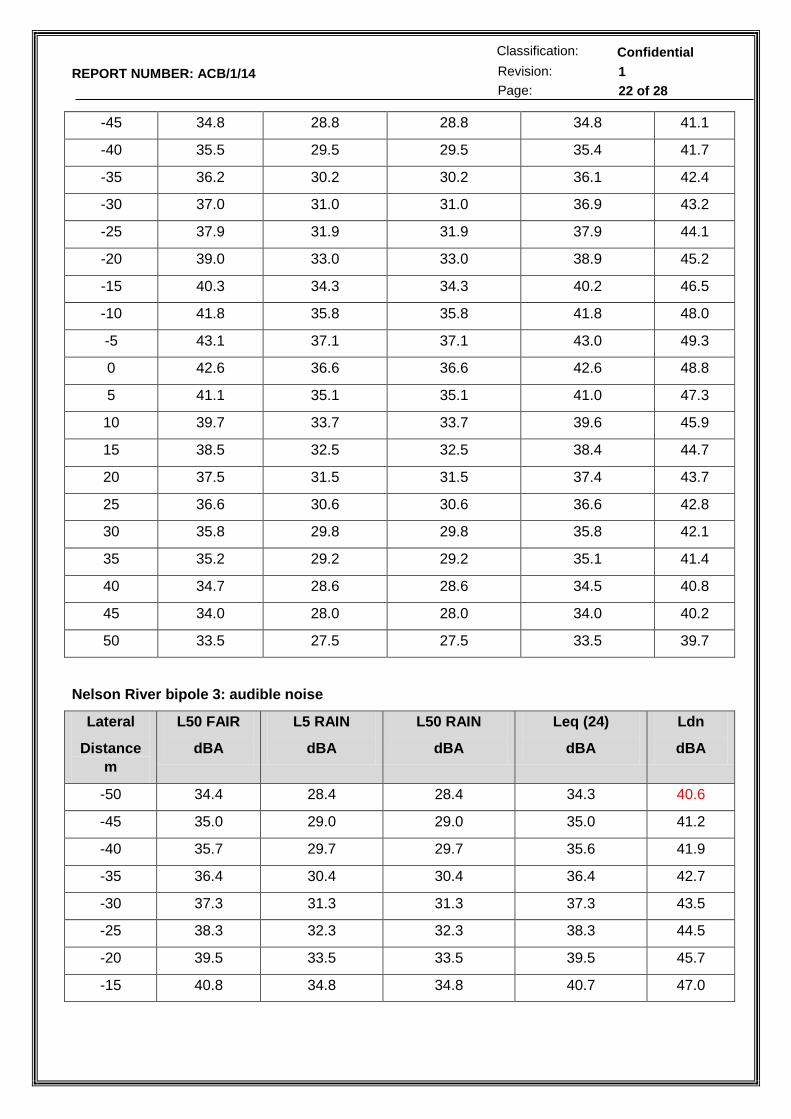
Audible noise case 2: 2x3.04 cm; lateral profile at midspan

Lateral

Distance m

L50 FAIR

dBA

L5 RAIN

dBA

L50 RAIN

dBA

Leq (24)

dBA

Ldn

dBA

-50 34.3 28.3 28.3 34.2 40.5


Confidential

Revision: 1

Page: 22 of 28

Classification:

-45 34.8 28.8 28.8 34.8 41.1

-40 35.5 29.5 29.5 35.4 41.7

-35 36.2 30.2 30.2 36.1 42.4

-30 37.0 31.0 31.0 36.9 43.2

-25 37.9 31.9 31.9 37.9 44.1

-20 39.0 33.0 33.0 38.9 45.2

-15 40.3 34.3 34.3 40.2 46.5

-10 41.8 35.8 35.8 41.8 48.0

-5 43.1 37.1 37.1 43.0 49.3

0 42.6 36.6 36.6 42.6 48.8

5 41.1 35.1 35.1 41.0 47.3

10 39.7 33.7 33.7 39.6 45.9

15 38.5 32.5 32.5 38.4 44.7

20 37.5 31.5 31.5 37.4 43.7

25 36.6 30.6 30.6 36.6 42.8

30 35.8 29.8 29.8 35.8 42.1

35 35.2 29.2 29.2 35.1 41.4

40 34.7 28.6 28.6 34.5 40.8

45 34.0 28.0 28.0 34.0 40.2

50 33.5 27.5 27.5 33.5 39.7

Nelson River bipole 3: audible noise

Lateral

Distance

m

L50 FAIR

dBA

L5 RAIN

dBA

L50 RAIN

dBA

Leq (24)

dBA

Ldn

dBA

-50 34.4 28.4 28.4 34.3 40.6

-45 35.0 29.0 29.0 35.0 41.2

-40 35.7 29.7 29.7 35.6 41.9

-35 36.4 30.4 30.4 36.4 42.7

-30 37.3 31.3 31.3 37.3 43.5

-25 38.3 32.3 32.3 38.3 44.5

-20 39.5 33.5 33.5 39.5 45.7

-15 40.8 34.8 34.8 40.7 47.0


Confidential

Revision: 1

Page: 23 of 28

Classification:

-10 41.8 35.7 35.7 41.8 48.0

-5 41.7 35.7 35.7 41.7 47.9

0 0 34.6 34.6 46.9 46.9

5 39.4 33.4 33.4 39.3 45.6

10 38.2 32.2 32.2 38.2 44.4

15 37.2 31.2 31.2 37.2 43.4

20 36.4 30.4 30.4 36.3 42.6

25 35.6 29.6 29.6 35.6 41.8

30 34.9 28.9 28.9 34.9 41.1

35 34.3 28.3 28.3 34.8 40.5

40 33.8 27.8 27.8 33.7 40.0

45 33.2 27.2 27.2 33.2 39.5

50 32.8 26.8 26.8 32.7 39.0

ELELCTRIC FIELD STUDIES

1x4.44 cm conductor, balanced voltage

Lateral

Distance

m

DC

ELECTROST

ATIC FIELD

Em

kV/m

MAXIMUM

FAIR

WEATHER

FIELD WITH

SPACE

CHARGE

kV/m

ELECTRIC

FIELD L50 IN

RAIN kV/m

Ion current

density

nA/m2

Ion

density

Ions/cm3

/-50 0.21 2.32 1.5 0.1 2984

-45 0.28 2.78 1.8 0.2 3947

-40 0.39 3.37 2.2 0.3 5335

-35 0.55 4.17 2.8 0.6 7436

-30 0.84 5.23 3.6 1.0 10676

-25 1.33 6.80 4.7 2.0 16122

-20 2.23 9.04 6.5 4.2 25270

-15 3.93 12.49 9.3 8.1 35135

-10 6.68 20.13 15.0 28.7 77585

-5 7.08 21.93 16.3 52.0 128802

0 0 0.03 0 0 0

5 -7.08 -21.93 -16.3 -67 -128802


Confidential

Revision: 1

Page: 24 of 28

Classification:

10 -6.68 -20.13 -15.0 -37.5 -77585

15 -3.93 -12.49 -9.3 -10.5 -35136

20 -2.23 -9.04 -6.5 -5.5 -25270

25 -1.33 -6.80 -4.7 -2.6 -16122

30 -0.84 -5.23 -3.6 -1.3 -10676

35 -0.55 -4.17 -2.8 -0.7 -7436

40 -0.39 -3.37 -2.2 -0.4 -5335

45 -0.28 -2.78 -1.8 -0.3 -3947

50 -0.21 -2.32 -1.5 -0.2 -2984

2x3.04 cm conductor

Lateral

Distance

m

DC

ELECTROST

ATIC FIELD

Em

kV/m

MAXIMUM

FAIR

WEATHER

FIELD WITH

SPACE

CHARGE

kV/m

ELECTRIC

FIELD L50 IN

RAIN kV/m

Ion

current

Density

nA/m2

Ion

density

Ions/cm3

-50 0.26 2.32 1.5 0.1 2984

-45 0.34 2.78 1.8 0.2 3947

-40 0.48 2.37 2.2 0.3 5335

-35 0.69 4.17 2.8 0.6 7436

-30 1.04 5.23 3.6 1.0 10676

-25 1.65 6.80 4.8 2.0 16122

-20 2.77 9.03 6.6 4.2 25270

-15 4.88 12.50 9.5 8.1 34941

-10 8.29 20.1 15.5 28.4 76753

-5 8.71 21.41 16.5 49.7 125035

0 0.0 -0.03 0 0 0

5 -8.71 -21.41 -16.5 -64 -125035

10 -8.29 -20.01 -15.5 -37 -76753

15 -4.88 -12.5 -9.5 -10 -34941

20 -2.77 -9.03 -6.6 -5.5 -25270

25 -1.65 -6.80 -4.8 -2.6 -16122

30 -1.04 -5.23 -3.6 -1.3 -10676


Confidential

Revision: 1

Page: 25 of 28

Classification:

35 -0.69 -4.17 -2.8 -0.7 -7436

40 -0.48 -3.37 -2.2 -0.4 -5335

45 -0.34 -2.78 -1.8 -0.3 -3947

50 -0.26 -2.32 -1.5 -0.2 --2984

Bipole 3: Electric field and ion concentrations for a bipolar voltage of ±500 kV

Lateral

Distance

m

DC

ELECTRO

STATIC

FIELD Em

kV/m

MAXIMUM

FAIR

WEATHER

FIELD WITH

SPACE

CHARGE

kV/m

ELECTRIC

FIELD L50

IN RAIN

kV/m

Ion current

density

nA/m2

Ion density

Ions/cm3

-50 0.57 6.73 4.2 0.8 6781

-45 0.77 8.06 5.1 1.3 9004

-40 1.08 9.98 6.4 2.3 12522

-35 1.57 12.53 8.1 4.2 17932

-30 2.38 16.31 10.7 8.2 27121

-25 3.81 21.95 14.6 17.7 43526

-20 6.39 30.92 21.0 43.1 75296

-15 10.63 43.65 30.3 107.9 133608

-10 14.6 54.93 38.6 209.1 206335

-5 11.07 46.37 32.1 176.7 207481

0 0.00 0.05 0.00 -1.2 -12

5 -11.14 -46.37 -32.2 -232.1 -207481

10 -14.56 -54.87 -38.6 -272 -206335

15 -10.52 -43.32 -30.3 -139 -133608

20 -4.82 -23.76 -21.0 -55.8 -75296

25 -3.73 -21.44 -14.6 -22.9 -43526

30 -2.36 -16.14 -10.7 -10.6 -27121

35 -1.55 -12.46 -8.1 -5.4 -17932

40 -1.07 -9.93 -6.4 -3.0 -12522

45 -0.76 -8.03 -5.1 -1.7 -9004

50 -0.57 -6.71 -4.2 -1.1 -6781


Confidential

Revision: 1

Page: 26 of 28

Classification:

VOLTAGE UNBALANCE

Influence of the common mode voltage unbalance on the conductor surface gradients,

ground level electric field and audible noise (1x4.44 cm conductor)

VOLTAGE

UNBALANCE

±%

POLE

VOLTAGES

kV

ES1,2

kV/cm

EP

kV/cm

EMAX

kV/m

Ldn

dBA @ 30

m (ROW)

0 (NORMAL) +320

-320

-10.4

+10.3

+22.3

+22.9

21.9 46.7

47.9

5 +336

-304

+304

-336

-9.4

+11.3

+9.4

-11.3

-23.1

-24.3

+23.1

+24.3

-25.6

+23.7

44.9

46.0

48.5

49.7

6 +339

-301

+301

-339

-11.5

+9.2

-9.2

+11.5

+23.9

-21.9

-23.9

+21.9

+24.1

-4.1

48.8

50.0

45.7

44.6

8 +347

-294

+294

-347

+8.7

-12.0

-8.7

+12.0

+24.3

-21.6

-21.6

-24.3

-25.0

25.0

49.7

50.9

43.8

44.9

10

+352

+288

+352

-288

-8.4

+12.3

+8.4

-12.3

+24.27

21.57

+23.7

+24.5

-25.4

+25.6

44.2

51.4

15

+368

-272

+272

-368

+7.3

-13.3

-7.4

+13.3

+25.3

-20.4

+20.3

-25.3

+27.8

-27.8

53.0

51.9

42.2

41.1

20 +384

-256

+256

-384

-14.30

+6.37

-6.37

+14.32

+26.2

-19.6

+19.6

-26.2

+29.7

-29.7

53.5

54.7

39.0

40.2


Confidential

Revision: 1

Page: 27 of 28

Classification:

25 +400

-240

+240

-400

-15.3

+5.4

-5.4

+15.3

+27.0

-18.9

+18.9

-27.0

+31.6

-31.6

55.1

56.2

37.1

38.1

Influence of the common mode voltage unbalance on the conductor surface gradients,

ground level electric field and audible noise (2x3.04 cm conductors)

VOLTAGE

UNBALANCE

±%

POLE

VOLTAGES

kV

ES1,2

kV/cm

EP

kV/cm

EMAX

kV/m

Ldn

dBA @ 30

m (ROW)

0 (NORMAL) +320

-320

-10.4

+10.3

+22.3

+22.9

21.9 46.7

47.9

5 +336

-304

+304

-336

-9.4

+11.3

+9.4

-11.3

-23.1

-24.3

+23.1

+24.3

-25.6

+23.7

44.9

46.0

48.5

49.7

6 +339

-301

+301

-339

-11.5

+9.2

-9.2

+11.5

+23.9

-21.9

-23.9

+21.9

+24.1

-24.1

48.8

50.0

45.7

44.6

8 +347

-294

+294

-347

+8.7

-12.0

-8.7

+12.0

+24.3

-21.6

-21.6

-24.3

-25.0

25.0

49.7

50.9

43.8

44.9

10

+352

+288

+352

-288

-8.4

+12.3

+8.4

-12.3

+24.2

+21.5

+23.7

+24.5

-25.4

+25.6

44.2

51.4

15

+368

-272

+272

+7.3

-13.3

-7.4

+25.3

-20.4

+20.3

+27.8

-27.8

53.0

51.9

42.2


Confidential

Revision: 1

Page: 28 of 28

Classification:

-368 +13.3 -25.3 41.1

20 +384

-256

+256

-384

-14.30

+6.37

-6.37

+14.32

+26.2

-19.6

+19.6

-26.2

+29.7

-29.7

53.5

54.7

39.0

40.2

25 +400

-240

+240

-400

-15.3

+5.4

-5.4

+15.3

+27.0

-18.9

+18.9

-27.0

+31.6

-31.6

55.1

56.2

37.1

38.1

Compact HVDC ±320 kV lines proposed for the Nelson River...

Documents

Transcript of Compact HVDC ±320 kV lines proposed for the Nelson River...