Comovement and Predictability Relationships

Between Bonds and the Cross-Section of Stocks

Malcolm Baker Harvard Business School and NBER

mbaker@hbs.edu

Jeffrey Wurgler NYU Stern School of Business and NBER

jwurgler@stern.nyu.edu

December 12, 2011

Abstract

Government bonds comove more strongly with bond-like stocks: stocks of large, mature, low-volatility, profitable, dividend-paying firms that are neither high growth nor distressed. Variables that are derived from the yield curve that are already known to predict returns on bonds also predict returns on bond-like stocks; investor sentiment, a predictor of the cross-section of stock returns, also predicts excess bond returns. These relationships remain in place even when bonds and stocks become “decoupled” at the index level. They are driven by a combination of effects including correlations between real cash flows on bonds and bond-like stocks, correlations between their risk-based return premia, and periodic flights to quality.

We appreciate helpful comments from editor Jeff Pontiff, anonymous referees, Vito Gala, Robin Greenwood, Pascal Maenhoet, Stefan Nagel, Stijn Van Nieuwerburgh, Geoff Verter, and Pierre-Olivier Weill, and participants of seminars at the American Finance Association 2010 meeting, Barclays Global Investors, Cornell University, Drexel University, the Federal Reserve Bank of New York, the National Bureau of Economic Research, Northwestern University, UC Davis, UCLA, Temple University, the University of Texas at Austin, the University of Toronto, and Stanford University. We thank the Investment Company Institute for data on mutual fund flows. Baker gratefully acknowledges financial support from the Division of Research of the Harvard Business School.

Comovement and Predictability Relationships

Between Bonds and the Cross-Section of Stocks

Abstract

Government bonds comove more strongly with bond-like stocks: stocks of large, mature, low-volatility, profitable, dividend-paying firms that are neither high growth nor distressed. Variables that are derived from the yield curve that are already known to predict returns on bonds also predict returns on bond-like stocks; investor sentiment, a predictor of the cross-section of stock returns, also predicts excess bond returns. These relationships remain in place even when bonds and stocks become “decoupled” at the index level. They are driven by a combination of effects including correlations between real cash flows on bonds and bond-like stocks, correlations between their risk-based return premia, and periodic flights to quality.

1

I. Introduction

The empirical relationships between the stock and bond markets are of considerable

interest to economists, policymakers, and investors. Economists are interested in understanding

the mechanisms that link these markets. Through such understanding, financial market regulators

aim to improve the markets' information aggregation and capital allocation functions and their

robustness to shocks to the financial system. Investors want to know the return and

diversification properties of major asset classes.

The relationships between stock and bond returns have proved difficult to pin down,

however, let alone to understand. Over the last four decades, the correlation between stock index

and government bond returns has been highly unstable. Baele, Bekaert, and Inghelbrecht (2009),

for example, find that the correlation between daily returns on stock and bond indices is on

average modestly positive but has ranged anywhere from +0.60 to -0.60 over the last forty years

and exhibits sharp changes of 0.20 or more from month to month. In negative correlation periods

the markets are sometimes said to have “decoupled.” Many attempts have been made to explain

this time variation, but no consensus exists, and the literatures on stock and bond pricing remain

rather decoupled as well.

In this paper we look at these two markets from a different perspective. We document

and discuss the links between government bonds and the cross-section of stocks. Prior research

has focused almost exclusively on index-level time-series relationships. The cross-sectional

perspective complements this research, and it uncovers new and robust facts about the

connections between stocks and bonds.

The paper has three parts. The first studies the contemporaneous comovement patterns

between bonds and the (time-series of) the cross-section. The second part studies the

2

predictability patterns common to excess government bond returns and the cross-section. The

third part considers explanations for the patterns that we document. It concludes that at least

three mechanisms play a nonzero role.

The main comovement pattern between government bonds and the cross-section of stocks

is quite intuitive: bonds comove more strongly with “bond-like” stocks. Large stocks, long-listed

stocks, low volatility stocks, stocks of profitable and dividend-paying firms, and stocks of firms

with mediocre growth opportunities are more positively correlated with government bonds—

controlling for overall stock market returns. This control is important, because it allows us to

separate stable cross-sectional relationships from time-varying aggregate correlations. Stocks of

smaller, younger firms, highly volatile stocks, and stocks of firms with extremely strong growth

opportunities or those in distress, display a considerably weaker link to bonds—again,

controlling for overall stock market returns. These patterns remain even when bonds and stock

indices are moving in opposite directions. Thus, while so-called decoupling episodes are

dramatic and undoubtedly worthy of attention, there remain basic links between stocks and

bonds that are unaffected even in such extreme periods.

Bonds and bond-like stocks also exhibit similar predictability characteristics. The same

yield curve variables often used to predict returns on government bonds, such as the term spread

and combinations of forward rates (Fama and French (1989), Campbell and Shiller (1991), and

Cochrane and Piazzesi (2005)), also predict the returns on bond-like stocks relative to

speculative stocks.1 In the other direction, the sentiment index that Baker and Wurgler (2006) use

to predict the returns on bond-like relative to speculative stocks also predicts the returns on

government bonds. This cross-sectional focus complements Fama and French's stock-index-level

tests and delivers strong evidence that the expected returns of stocks and bonds are firmly linked. 1 A fuller literature review follows this introductory section.

3

We offer a preliminary assessment of the drivers of these patterns. We consider three

general, non-exclusive reasons why bonds would be more closely linked to some stocks than

others. They involve cash flows, risk-based required returns, and flights to quality or investor

sentiment. These have all been suggested and studied before but not in the cross-sectional

context, which provides some additional power to assess their relevance. We believe that it is

simply not possible to provide a complete, unambiguous attribution across these forces, because

so many untestable structural assumptions would need to be made. We therefore pursue a more

realistic goal, asking whether each should be given zero or nonzero weight in the results.

Since bonds and bond-like stocks are clearly exposed to common shocks to real cash

flows, we assign positive weight to the cash flow channel immediately. More interesting and

difficult is the task of disentangling and assessing the risk-based required returns and investor

sentiment channels. The bond-cross-section predictability connections indicate that at least one

of these also must be given nonzero weight. Risk-based required returns suggests a degree of

predictability, as does any predictable correction of periodic flights to quality or drifts away from

quality in which investors reallocate without a sophisticated eye toward risks and expected

returns.

There is evidence that both of these mechanisms play a role. The risk-based required

returns channel explains the stylized facts as the result of bonds and bond-like stocks (relative to

speculative stocks) being subject to common, risk-based discount rate shocks. This implies either

that betas or market risk premia vary over time with the bond and stock predictors. We test for

time-varying market betas directly and find a change in the right direction, with betas of bond-

like stocks falling when predicted bond returns are low. However, the betas do not change by

nearly enough to generate the observed magnitude of predictability with a constant market risk

4

premium of plausible magnitude. The time-varying risk premium is also unable to provide a

complete explanation, particularly for the fact that higher beta or other categories of speculative

firms are often predicted to have lower returns than presumably lower-risk stocks.

The investor sentiment channel explains the comovement evidence as sentiment affecting

bonds and bond-like stocks less intensively than it does speculative stocks, and the predictability

evidence as the somewhat forecastable correction of overreaction. We consider this story from

multiple angles. We observe that sentiment and flights to quality are anecdotally associated with

a number of special financial market episodes, including but not limited to the stock market

decline of 2008. More rigorously, periodic overreaction can explain the pattern that the riskiest

stocks are, not infrequently, poised to deliver the lowest expected returns. In addition, we

conduct a calibration in the spirit of Campbell and Thompson (2007) that suggests that bond

returns are simply too predictable to be consistent with fully efficient markets. Finally, we factor

analyze mutual fund flows across fund categories as in Goetzmann, Massa, and Rouwenhorst

(2000) and uncover an important factor consistent with flights to quality.

To summarize, there are intuitive cross-sectional differences in the comovement of

government bonds and stocks; these patterns are stable even when index-level comovement

relationships break down; bonds and bond-like stocks also exhibit related predictability patterns;

and it appears that at least three economic mechanisms are playing a role in the results.

Section II provides an overview of related literature. Section III describes the data and

studies the comovement relationships between government bonds and the cross-section of stocks.

Section IV studies predictability. Section V discusses interpretations and Section VI concludes.

II. Related literature

5

There is a substantial prior literature that studies stocks and government bonds. As

mentioned above, it commonly focuses on stock indices. Fama and Schwert (1977), Keim and

Stambaugh (1986), and Campbell and Shiller (1987) started a literature that used dividend yields

and interest rates to forecast stock and bond index returns. Using the term spread, the default

spread, and the dividend yield, for example, Fama and French (1989) find common predictable

components in bond and stock indices. Shiller and Beltratti (1992) and Campbell and Ammer

(1993) use present-value relations in an effort to decompose stock and bond index returns into

shocks related to real cash flows and discount rates. Recent contributions include Baele, Bekaert,

and Inghelbrecht (2009), Bekaert, Engstrom, and Grenadier (2005), and Campbell, Sunderam,

and Viceira (2009). Our methodology controls for the time-varying aggregate correlation and

looks for stable correlations within the cross-section, so in that sense our results do not have

immediate implications for the aggregate puzzle (but we do describe an effort to connect it to

that puzzle later on).

Exceptions to an exclusive focus on stock indices include Fama and French (1993) and,

more recently, Koijen, Lustig, and Van Nieuwerburgh (2010). Among other findings in their

paper, Fama and French document that the term spread and the default spread have strong

contemporaneous relationships to several size- and book-to-market-based stock portfolios. They

do not develop or interpret the cross-sectional differences in the relationships, however, as their

emphasis is on covariances between yield-curve variables and various stock portfolios.

Koijen et al. is also complementary. They develop a no-arbitrage model that prices stocks

and bonds, with a cross-sectional focus on size and book-to-market portfolios. On the bond

market side, we use a simpler empirical approach, and we come to different conclusions because

6

we focus on a broader set of stock portfolios and a broader set of bond market predictors.2 On the

stock market side, Koijen et al. use the dividend-price ratio as an aggregate predictor of interest.

Because we focus on other sorts, and the dividend-price ratio has little explanatory power for the

cross-section, we focus on investor sentiment as the connection between the markets. Sentiment

has been more empirically successful in the prior literature and, it turns out, in this paper as well.

Our paper also relates to literature that considers how shifting sentiment or flights to

quality influence predictability results. Connolly, Stivers, and Sun (2005) show that bond returns

tend to be high relative to stock index returns when the implied volatility of equity index options

increases. Gulko (2002) was among the first to document the decoupling phenomenon in

showing that the unconditional positive correlation between stocks and bonds switches sign in

stock market crashes. Lan (2008) also observes this phenomenon and uses a Campbell-Shiller

(1988) decomposition to study how time-varying expectations of cash flow and risk premia may

contribute to it. Beber, Brandt, and Kavajecz (2009) find traces of flights to quality and flights to

liquidity in the Euro-Area bond market. Implicit in some of these results is the notion of

mispricing in the bond market, such as is argued for by the predictability associated with

relatively exogenous government bond supply shocks in Greenwood and Vayanos (2010a,b).

Gabaix (2010) develops a model where perceptions of risks (modeled as perceptions of behavior

during disasters) affect stocks and bonds systematically. He suggests a way to think

quantitatively about the joint behavior of sentiment and prices.

This literature highlights another difference between our paper and Fama and French

(1993) and Koijen et al. (2010). These papers do not look specifically at decoupling periods,

which have reemerged as an area of interest after the market meltdowns that began in the autumn

2 Like Koijen et al., we do not find that the level of CP predicts the value premium unconditionally. Looking forward, we do find that it predicts volatility and real growth (sales, assets) sorted portfolios, as well as book-to-market portfolios sorted non-monotoniccally.

7

of 2008. We study these patterns specifically, and find some additional links between bonds and

the cross-section of stocks that do not appear in the aggregate stock-bond relationship.

III. Comovement of bonds and the cross-section of stocks

To characterize how the cross-section of stock returns covaries with bond returns, we

study a broad range of stock portfolios, including those formed on firm size, firm age (period

since first listing on a major exchange), profitability, dividend policy, and growth opportunities

and/or distress. We first describe the data and then the basic regression results.

A. Data on stock and bond indices and stock portfolios

Table 1 summarizes stock and bond index data. Monthly excess returns on intermediate-

term government bonds and long-term government bonds are constructed using data from

Ibbotson Associates (2011). Monthly excess returns on the value-weighted NYSE/Amex/Nasdaq

stock market are from CRSP.3

The stock portfolio constructions follow Fama and French (1992) and Baker and Wurgler

(2006). The firm-level data is from the merged CRSP-Compustat database. The sample includes

all common stock (share codes 10 and 11) between 1963 and 2010. As discussed in Fama and

French (1992), Compustat data prior to this date has major selection bias problems, being biased

toward large and historically successful firms. Accounting data for fiscal year-ends in calendar

year t-1 are matched to monthly returns from July t through June t+1. We omit summary

statistics on unconditional returns to save space. We are interested in conditional patterns in any

event. They are similar to those reported in Baker and Wurgler (2006) for the same portfolios.

3 We do not consider corporate bonds because they are spanned by government bonds and the wide cross-section of stocks in the comovement characteristics that we study. High-grade corporate bonds behave more like government bonds, while junk bonds behave somewehat more like speculative stocks.

8

Size and age characteristics include market equity ME from June of year t, measured as

price times shares outstanding from CRSP. ME is matched to monthly returns from July of year t

through June of year t+1. Age is the number of years since the firm’s first appearance on CRSP,

measured to the nearest month. Return volatility, denoted by , is the standard deviation of (raw)

monthly returns over the twelve months ending in June of year t. If there are at least nine returns

to estimate it, is matched to monthly returns from July of year t through June of year t+1.

Profitability is measured by the return on equity E/BE. Earnings (E) is income before

extraordinary items (Item 18) plus income statement deferred taxes (Item 50) minus preferred

dividends (Item 19), if earnings are positive; book equity (BE) is shareholders equity (Item 60)

plus balance sheet deferred taxes (Item 35). Dividends are dividends to equity D/BE, which is

dividends per share at the ex date (Item 26) times Compustat shares outstanding (Item 25)

divided by book equity. For dividends and profitability, there is a salient distinction at zero, so

we split dividend payers and profitable firms into deciles and study nonpayers and unprofitable

firms separately.

Characteristics indicating growth opportunities, distress, or both include book-to-market

equity BE/ME, whose elements are defined above. External finance EF/A is the change in assets

(Item 6) minus the change in retained earnings (Item 36) divided by assets. Sales growth (GS) is

the change in net sales (Item 12) divided by prior-year net sales.

The growth and distress variables reflect several effects simultaneously. With book-to-

market, high values are often associated with distress and low values with high growth

opportunities. Likewise, low values of sales growth and external finance (i.e., negative numbers)

can indicate distress, while high values may reflect growth opportunities. In other words,

although these portfolios are often considered in a simple “high minus low” sense, a closer look

9

suggests that the extremes include relatively more speculative stocks, in contrast to the middle

deciles which tilt toward less speculative stocks. Complicating matters further, book-to-market is

a generic valuation indicator, varying with any source of mispricing or risk-based required

returns. Similarly, to the extent that external finance is driven by investor demand and/or market

timing, it also serves as a generic misvaluation indicator.

We use equal-weighted stock portfolios. Using value-weighted portfolios would obscure

the relationships and contrasts of interest. Some of the cells would be dominated by a few large

cap stocks, reducing power, and focusing on the stocks within each group that are already more

bond-like. This would move our estimates toward zero. Instead, we will control for size effects

through regression and double sorts to determine that the results go beyond size alone.

B. Comovement patterns

Table 2 reports the basic comovement results. The approach is to regress monthly excess

stock portfolio returns on contemporaneous excess long-term bond returns while controlling for

overall stock market returns (portfolio market beta):

ptftbtpftmtppftpt urrbrrarr . (1)

The inclusion of overall stock market returns in this regression allows us to isolate cross-

sectional differences in “bond beta” without confusing them with the average correlation

between the aggregate stock market and bonds. The top panel shows the cross-section of stock

market beta loadings p. This mainly provides some intuition about the composition of the

portfolios. We focus on the coefficient bp, which tells us the relationship between stock portfolio

p and government bonds that arises over and above their relationship through general stock

market movements.

10

The bottom panels of Table 2 reveal a novel but intuitive comovement pattern. Generally

speaking, portfolios of “bond-like” stocks—stocks with the characteristics of safety as opposed

to risk and opportunity—show higher partial correlations with long-term bond returns. Such

bond-like stocks include large stocks, low-volatility stocks, and high-dividend stocks. The

maximum coefficient in Panel B is the 0.13 on the lowest-volatility stocks. In other words, a one

percentage point higher excess return on long-term bonds is associated with a 0.13 percentage

point higher monthly excess return on low-volatility stocks, all controlling for general stock

market returns. The second-largest coefficients involve stocks paying high dividends relative to

book equity. The relationship is not monotonic across the top deciles, however, possibly because

some stocks with very low equity may actually be in distress.

The converse is that stocks that are relatively more “speculative” are relatively less

connected to bonds. Small-capitalization stocks, young stocks, high-volatility stocks, non-

dividend paying stocks, and unprofitable stocks all display strongly negative coefficients bp. The

minimum coefficient of -0.43 is on the unprofitable stocks portfolio; a one percentage point

higher excess return on long-term bonds is associated with a 0.43 percentage point lower excess

return on unprofitable stocks, controlling for general stock market returns. The second-lowest

coefficient in the table is the -0.41 coefficient on the most volatile stocks.

The bottom three rows in Panel B suggest an interesting U-shaped pattern in the growth

and distress variables’ coefficients. The interpretation is intuitive; both high growth and

distressed firms are less like bonds than are the stable and mature firms in the middle deciles.

This U-shaped pattern mirrors that discussed in Baker and Wurgler (2006, 2007), who find that

both high growth and distressed stocks are more sensitive to sentiment than more staid firms.

11

The pattern also suggests that simple high-minus-low portfolios can hide key aspects of the

cross-section, including those in the oft-studied book-to-market portfolios.

The stock characteristics examined here are correlated, so a natural question is the extent

to which they embody independent effects. To examine this question, the left panels of Figure 1

plot the coefficients across stock deciles bp, as reported in Table 2, while the middle panels plot

the coefficients bp that are estimated (but not reported in a table) after adding Fama and French’s

(1993) factors SMB and HML and the momentum factor UMD to Eq. (1). As expected, the

patterns are attenuated by the inclusion of the additional stock portfolios, but remain qualitatively

identical in every portfolio.

Another way of examining the degree of independence of the effects in Table 2 is

through a double sort methodology. In particular, many of the characteristics we examine are

correlated with firm size, so we perform separate regressions within each size quintile and

compute the average coefficient on long-term bonds across the five quintiles. The right panels of

Figure 1 show these average coefficients. Again, the pattern is similar.

In unreported results, we repeat Table 2 separately for two samples, one for firms above

the median profitability for the NYSE and one for firms below. This amounts to a double sort.

We can ask, for example, whether a profitable growth stock (or value stock) is more bond-like

than a generic growth stock. Rather than clear interactions, however, the predominant effect is

simply that profitable firms have stronger comovement relationships with bonds than

unprofitable firms in every characteristic-decile cell. Otherwise, the same qualitative patterns

appear in both halves of the sample.

C. Comovement in “decoupling” episodes

12

As mentioned in the Introduction, the correlation between government bonds and stock

indices is well-known to be highly unstable. For example, Baele, Bekaert, and Inghelbrecht

(2010) show that within our own sample period the correlation between indices has ranged from

over +0.60 to below -0.60. Where the correlation switches from positive to negative it is

sometimes said to have “decoupled.”

A number of authors have studied this variation. Gulko (2002) finds that decoupling is

associated with steep stock market declines, and, relatedly, Connolly, Stivers, and Sun (2005)

find that the correlation falls when the implied volatility of equity index options rises, which also

happens during market declines. Baele, Bekaert, and Inghelbrecht conclude that time variation is

driven more by liquidity and flight-to-quality factors than by changing macroeconomic

fundamentals, and Bansal, Connolly, and Stivers (2009) also find links to liquidity. Campbell,

Sunderam, and Viceira (2009) propose an explanation that includes an associated time-varying

covariance between inflation and real shocks.

A natural question is whether the cross-sectional comovement patterns documented

earlier exhibit similar instability. Table 3 explores this question under definitions of

“decoupling” suited to our monthly data. We use long-short portfolios rather than deciles to save

space. In Panel A, we confirm that the bond-cross-section patterns from Table 2 are clearly

apparent in the somewhat more common “coupling” regime in which bonds and stock indexes

move in the same direction.

Panel B shows that not a single one of these patterns reverses when bonds and stock

indexes move in opposite directions. Most remain statistically significant, including those that

are also of relatively high magnitude in the coupling regime: volatility, size, and dividends. Panel

C imposes an even stricter definition of decoupling, requiring that bonds and stocks move in

13

opposite directions in each of the two prior months. Here, too, none of the patterns reverse.

Indeed, several become stronger in economic and statistical significance than under the looser

definition of decoupling, and despite a much smaller sample size.

To summarize, this section documents a simple and robust stylized fact about

comovement between bonds and stocks: relative to speculative stocks, bond-like stocks comove

more closely with bonds. Our evidence suggests that the stock characteristics most closely

associated with bonds are low volatility, large size, seasoned age of listing, and high dividends.

Connections also exist between bonds and stocks with high profitability and neither high growth

nor distress. These cross-sectional relationships remain highly stable even when the correlation

between bonds and stock indices inverts.

D. On the relationship with aggregate stock-bond comovement

As noted before, Equation (1) divorces our analysis from the aggregate stock-bond

comovement puzzle. But our results raise the possibility that the time-varying aggregate

correlation reflects a composition effect—for example, if IPOs flood the market or existing

stocks become more volatile, and less bond-like, then we would expect the aggregate stock

market relationship with bonds to deteriorate. To explore this, we tracked a five-year rolling

average of the median total volatility across individual stocks—our strongest results are for

volatility portfolios—and compared this to the five-year rolling average of the monthly

covariance between stock market and bond returns. Unfortunately, outside of a window around

the Internet bubble, the relationship is not as consistently negative as would seem to be required

to explain the time-varying aggregate correlation via a sample composition effect.

IV. Predictability of bonds and the cross-section of stocks

14

The comovement patterns provide us with new stylized facts, but sheds no light on their

drivers. In this section, we study whether bond returns and bond-like stock returns are

predictable using the same variables. The analysis adds more new facts that are interesting in

their own right. It also allows us to begin to assess the causes of the comovement patterns.

Specifically, this sort of “overlapping” predictability is implied by only two of the three

categories of potential causes of comovement: time-variation in risk-based required returns, if

the predictor captures a state variable related to risk premia; and, the correction of sentiment-

driven mispricings, if the predictor captures the state of sentiment. In other words, the absence of

overlapping predictability would, in a crude sense, rule out both of these channels, while the

presence of overlapping predictability would rule in at least one of them.

A. Data on predictors

We construct two types of time-series predictors: those that have been used primarily to

forecast bond returns, and one that has been used to forecast the time series of the cross-section

of stock returns. This involves several predictors drawn from several papers so the full data

description is not short.

Starting first with variables previously used to forecast excess bond returns, Fama and

Bliss (1987) and Cochrane and Piazzesi (2005) develop predictors based on forward rates.

Cochrane and Piazzesi find that a tent-shaped function of one- to five-year forward rates

forecasts bond returns. CPIT is the Cochrane-Piazzesi fitted predictor for intermediate term

excess bond returns, i.e. the fitted intermediate-term excess bond return using the 1-year rate and

the 2- through 5-year forward rates derived from the Fama-Bliss yield curve from CRSP in a

monthly forecasting regression. Note that we are interested in forecasting monthly returns, while

Cochrane and Piazzesi use their factor to forecast overlapping annual returns from month t+1

15

through month t+12. To be consistent with the spirit of their predictor, we use 12-month moving

averages of the forward rates in the predictive regression. Similarly, CPLT is the Cochrane-

Piazzesi fitted predictor for long-term excess bond returns fitted using the same set of interest

rates. The coefficients in the predictive regressions are reported in the header in Table 4,

confirming the established tent-shaped function of forward rates. The Cochrane-Piazzesi

variables are perhaps the strongest known predictors of bond returns.

Fama and French (1989) and Campbell and Shiller (1991) find that a large term spread

predicts higher excess bond returns. CSIT is the Campbell-Shiller-style fitted predictor of

intermediate excess bond returns using the risk-free rate, the term spread, the credit spread, and

the credit term spread. The risk-free rate is the yield on Treasury bills, and the term spread is the

difference between the long-term Treasury bond yield and the T-bill yield, both from Ibbotson

Associates (2008). The credit spread is the gap between the commercial paper yield and the T-

bill yield. The commercial paper yield series from the NBER website is based on Federal

Reserve Board data. The credit term spread is the difference between Moody’s Aaa bond yields,

also as reported by the Board, and the commercial paper yield. Each of the regressors is lagged

six months. Finally, CSLT is the Campbell-Shiller-style fitted predictor of long-term excess bond

returns using these variables. Again, we report the coefficients in the predictive regressions in the

header in Table 4, confirming known results such as the positive coefficients on the short-term

rate and the term spread.

There is a much smaller literature on predicting the time-series of the cross-section of

stock returns. One predictor is the investor sentiment index proposed in Baker and Wurgler

(2006). This is the predictor that we focus on, as they show it has predictive power across the full

range of portfolios that we consider. Finally, Ghosh and Constantinides (2011) estimate a

16

regime-switching model based on a nonlinear function of the risk-free rate and the market price-

dividend ratio and derive a model-implied factor to predict conditional cross-sectional returns.

Like Koijen et al., they focus on size and value portfolios.

The sentiment index is based on six underlying proxies for sentiment: the closed-end

fund discount as available from Neal and Wheatley (1998), CDA/Weisenberger, or the Wall

Street Journal; the number of and average first-day returns on IPOs from Jay Ritter’s website;

the dividend premium (the log difference between the value-weighted average market-to-book

ratio of dividend payers and nonpayers); the equity share in total equity and debt issues from the

Federal Reserve Bulletin; and detrended NYSE turnover (the log of the deviation from a 5-year

moving average). To further isolate the common sentiment component from common

macroeconomic components, each proxy was first orthogonalized to macroeconomic indicators,

including industrial production, the NBER recession indicator, and consumption growth.4 The

sentiment index SENT is the first principal component of the six orthogonalized proxies. It has

the expected pattern of positive loadings on the equity issuance and turnover variables and

negative loadings on the closed-end fund discount and the dividend premium. See Baker and

Wurgler (2006) for further construction details and motivation.

The sentiment index is a contrarian predictor. Baker and Wurgler (2006) find that when

the sentiment index takes high values, “high sentiment beta” stocks underperform over the next

year or more. Stocks with a high sentiment beta tend to be hard to arbitrage and hard to value

(speculative) stocks—for example, small, young, highly volatile, distressed, and rapid growth

stocks. These stocks are more prone to be mispriced when sentiment is highly bullish or bearish.

Their difficulty of valuation permits noise traders to entertain extreme valuations, and

4 The sentiment data are available at: www.stern.nyu.edu/~jwurgler.

17

simultaneously complicates the arbitrageurs’ task of identifying fundamental value. These same

stocks are also, generally speaking, more costly and risky to trade, which further discourages

arbitrageurs. As a result, high sentiment beta stocks are prone to be (relatively) overpriced when

sentiment is high and underperform going forward as prices correct, and vice-versa. We

hypothesize that bonds will perform more like low sentiment beta stocks. In a period of high

sentiment they may be relatively neglected and underpriced and perform better than average

going forward, and vice-versa.

Prior work tends to lag the yield curve predictors between one month, six months, and

one year in part as a result of the literature's cumulative outcome of empirical searches to

maximize bond return predictability. We have a similar decision here about how much to lag the

sentiment index. A combination of ex ante and Occam's razor considerations suggests one course

of action. As in the case of the cross-sectional variable momentum, there is a tension in the

dynamics of sentiment between short-term positive autocorrelation and long-term reversal. We

aim to focus on the latter to match the spirit of the yield curve predictors and the style of

predictability found in Baker and Wurgler (2006). We also prefer a round number that matches

how the majority of yield curve variables are handled. We therefore lag the index one year. We

denote this SENTlag.

An index that is simply lagged one year still has one undesirable property, namely that it

possesses significant monthly variation based on events that occurred between months t-11 and t-

12, for example sharp monthly changes in the number of IPOs and their market reception. This is

noise for the purposes of predictability from months t onward. To eliminate this but maintain the

index centered on t-12, we construct the moving average of SENTmonthly values from t-6 to t-

18. We denote this SENTsm. This balances several considerations and thus is the preferred

18

predictor based on investor sentiment. To facilitate interpretation all sentiment indices are

standardized after their construction.

Finally, we make use of a monthly index of changes in sentiment, SENT, which is

based on a similar principal components analysis of changes in the underlying sentiment proxies.

Our monthly sentiment series on this variable are as used in Baker and Wurgler (2007). As this is

employed only briefly as a control variable, we defer details of its construction to the header of

Table 4. Baker and Wurgler find that speculative, non-bond-like stocks possess higher sentiment

beta, i.e. higher contemporaneous sensitivity to this index.

The predictors are summarized in Table 4 and plotted in Figure 2. By construction, the

means of the fitted bond-return predictors match the means of the bond returns and the sentiment

indices have zero mean and unit variance by construction. The Cochrane-Piazzesi bond return

predictors are more variable than the Campbell-Shiller predictors, reflecting their better

forecasting ability. Several predictors are positively correlated at the 1% level, although this is

overstated because all of the series are persistent. Nonetheless, these positive correlations already

suggest that the predictors may possess overlapping predictive ability. Suggesting correct lagging

treatment of the sentiment index, the lagged index is much more correlated with the yield curve

predictors than the contemporaneous index. Figure 2 indicates that the bond return predictors and

the sentiment index are most linked in the late-1970s through mid-1980s period in which bond

return volatility increased.

B. Bond predictors and the cross-section of stock returns

We first test whether bond return predictors are also effective in predicting the returns to

bond-like stocks relative to speculative stocks. Few papers have investigated this and with no

focus on cross-stock differences. Cochrane and Piazzesi (2005) find that their forecasting factor

19

is positively related to annual value-weighted stock returns but do not consider other stock

portfolios. Fama and French (1989) find that the term spread has similar predictive power for

equal- and value-weighted stock indices, but do not go deeper into the cross-section of stocks,

and furthermore we have more than 20 additional years of data to study.

In Table 5 we regress excess stock portfolio returns on contemporaneous excess market

returns and the Cochrane-Piazzesi forecast of long-term excess bond returns:

ptLTtpftmtppftpt uCPtrrarr 1 . (2)

The specification intentionally resembles that of Eq. (1). It tests whether the Cochrane-Piazzesi

predictor extends to portfolio p with a differentially higher or lower predictive coefficient for

stock portfolio p than for the value-weighted average market return. Varying p thereby tests for

cross-sectional differences in forecasting ability. Coefficient tp measures the percentage increase

in returns associated with a one-percentage-point increase in the predicted long-term bond return,

controlling for the value-weighted stock return.

Predictors of excess bond returns do indeed nicely apply to the cross-section of stock

returns in the hypothesized directions. When predicted bond returns are high, the returns on

bond-like stocks (large, established, low-volatility firms) are also higher than the value-weighted

average stock return; the returns of speculative stocks (small, young, nonpaying, unprofitable,

high-volatility, and high-growth and distressed) are generally significantly lower than the

average. While the conditional spread of returns in size portfolios, for example, As in the

comovement coefficients, the total return volatility characteristic produces the greatest spread of

coefficients, suggesting that it best aligns with the speculative vs. bond-like differentiation. Also

as before, the sales growth characteristic produces the most pronounced U-shaped pattern.

Again, this is consistent with extreme growth stocks and distressed stocks being less bond-like

20

than firms with steady sales growth. Interestingly, the tp coefficient estimates from Eq. (2) are

similar in sign but generally larger in magnitude than the bp coefficients estimated from Eq. (1).

This has an interesting interpretation. Stock returns are particularly sensitive to the predictable

component of bond returns.5

The predictive coefficients tp are plotted in Figure 3. The left panels plot tp across stock

deciles. The middle panels plot the coefficients that are estimated after adding controls SMB,

HML, and UMD to Eq. (2). The right panels plot the coefficients from double sorts that control

for firm size as described earlier. There is a quite similar qualitative relationship between the

cross-sectional patterns in Figure 3 and those in Figure 1. At least some of the comovement

patterns shown earlier derive from shared predictable components.

We use the bond predictors to forecast long-short portfolios in Table 6. We also control

for the SMB, HML, and UMD portfolios to study special predictive power for portfolio p. We

consider regressions that are variants of this general form:

ptLTtptptptpftmtppftpt uCPtMOMmSMBsHMLhrrarr 1 (3)

In Panel A, the dependent variables are top decile minus bottom decile long-short portfolio

returns for those characteristics for which there are monotonic patterns in their comovement and

predictive coefficients across deciles: size, firm age, volatility, dividend payment, and

profitability. In Panel B, we reduce noise by forming long-short portfolios as the top three minus

the bottom three deciles for these characteristics. We also form portfolios that may detect the U-

shaped patterns in comovement coefficients for growth and distress variables. We form such

5 Most of the t-statistics in Table 5 are not significantly different from zero. This is expected given the pattern of coefficients and is not inconsistent with theoretical predictions. For example, the sigma coefficients must pass through zero on their way from significantly positive to significantly negative. The main point is that in most portfolios, the coefficients are generally statistically significant at at least one extreme.

21

portfolios as the extreme three minus the middle two deciles, which intuitively should capture

the contrast between speculative and bond-like stocks.

The results indicate that the Cochrane-Piazzesi factor has incremental predictive power

for the top minus bottom portfolios formed on volatility and dividends, even controlling for

future SMB and therefore the predictable component of SMB. Contrasting the top three and

bottom three deciles tends to strengthen these effects; it brings profitability up to a marginally

significant coefficient. The middle minus extreme portfolios also generate the U-shaped pattern

that is identical to the pattern of comovement. When predicted bond returns are high, so are

predicted returns on steady, slow growing stocks relative to the more speculative high growth

and/or distressed stocks.

For brevity, we do not present parallel sets of results for the other bond predictors CPIT ,

CSIT, and CSLT, but they display very similar patterns. The takeaway here is that variables known

to predict bond returns directly extend to the cross-section of stocks. As a descriptive matter, this

substantially enlarges the known sources of predictable variation of the time-series of the cross-

section of stock returns. It is also intuitively consistent with the connection between the bond

predictors and the sentiment index in Figure 2, as high values of the sentiment index are known

to predict high returns on bond-like stocks relative to other stocks.

C. Bond-like stock predictors and bond returns

We now reverse the analysis. We study whether the investor sentiment index SENT,

which is known to predict the relative return on bond-like stocks and speculative stocks, also

predicts bond returns. We run versions of this predictive regression:

ttLTtts

ftmtftbt ucSENTbCPSENTrrarr

11 . (4)

22

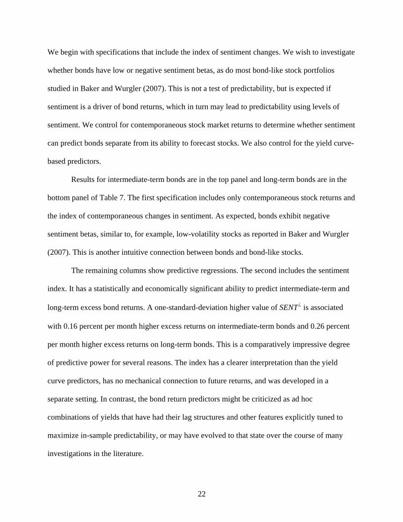
We begin with specifications that include the index of sentiment changes. We wish to investigate

whether bonds have low or negative sentiment betas, as do most bond-like stock portfolios

studied in Baker and Wurgler (2007). This is not a test of predictability, but is expected if

sentiment is a driver of bond returns, which in turn may lead to predictability using levels of

sentiment. We control for contemporaneous stock market returns to determine whether sentiment

can predict bonds separate from its ability to forecast stocks. We also control for the yield curve-

based predictors.

Results for intermediate-term bonds are in the top panel and long-term bonds are in the

bottom panel of Table 7. The first specification includes only contemporaneous stock returns and

the index of contemporaneous changes in sentiment. As expected, bonds exhibit negative

sentiment betas, similar to, for example, low-volatility stocks as reported in Baker and Wurgler

(2007). This is another intuitive connection between bonds and bond-like stocks.

The remaining columns show predictive regressions. The second includes the sentiment

index. It has a statistically and economically significant ability to predict intermediate-term and

long-term excess bond returns. A one-standard-deviation higher value of SENT is associated

with 0.16 percent per month higher excess returns on intermediate-term bonds and 0.26 percent

per month higher excess returns on long-term bonds. This is a comparatively impressive degree

of predictive power for several reasons. The index has a clearer interpretation than the yield

curve predictors, has no mechanical connection to future returns, and was developed in a

separate setting. In contrast, the bond return predictors might be criticized as ad hoc

combinations of yields that have had their lag structures and other features explicitly tuned to

maximize in-sample predictability, or may have evolved to that state over the course of many

investigations in the literature.

23

The third pair of columns uses a smoothed version of sentiment, averaging out the values

from six to 18 months prior to the return prediction. Theory provides little guidance to the lag

structure of the relationship between sentiment and future bond returns. We expect bond returns

to rise as sentiment falls from a high level back to average, but the speed of this mean reversion

is unclear. Another advantage of smoothing is that it irons out idiosyncratic jumps in the

underlying components of investor sentiment. Consistent with expectations, smoothing improves

the statistical and economic significance somewhat.

The last two sets of columns in each panel explore the independent predictive power of

the sentiment index and other bond return predictors. The overall message is that sentiment loses

predictive power when included alongside the strong Cochrane-Piazzesi predictor, although

remains marginally statistically significant, and is less affected by the Campbell-Shiller type

predictors. The inclusion of the sentiment index also tends to reduce the coefficient on the bond

predictors (below unity) and vice-versa. This is not a proper horse race, as the bond predictors

are overfit, having been pre-fitted over the same sample to maximize predictability, unlike the

sentiment index. However, for our analysis the interesting point is not that a particular variable

wins a horse race, but precisely the opposite—that the predictors do overlap to some degree. This

is consistent with the positive but moderate correlation in these series in Figure 2.

V. Discussion and interpretation

This paper's most concrete contribution is descriptive: bonds and bond-like stocks are

connected in both comovement and predictability patterns. As mentioned in the Introduction,

there are three general and non-exclusive causes of comovement between bonds and bond-like

stocks: comovement in their real cash flows, comovement in their risk-based required returns,

24

and common shocks to sentiment that affect bonds and bond-like stocks similarly. A convincing

quantitative attribution to these three causes is not possible, given the required structural

assumptions, and an approximate attribution is a sizeable endeavor best left for future work. In

this section we pursue the first step in that agenda. We try to assess whether one, two, or all three

mechanisms play a role in the results. At the end, we also comment on the relationship between

our results and the time-varying aggregate correlation between stocks and bonds.

A. Shocks to real cash flows

Bonds and bond-like stocks are linked through common shocks to real cash flows. Most

obviously, a business cycle contraction is often associated with lower inflation and rising bond

prices, and will generally have less of an impact on the cash flows of stable, mature firms versus

more speculative growth firms or already-distressed firms. For example, Chen, Roll, and Ross

(1986), find that a equal-weighted stock index is almost uniformly more affected by a range of

macroeconomic shocks, including to inflation, than a value-weighted index. Such effects would

contribute to the relatively stronger comovement between bonds and bond-like stocks.

Subsequent studies in the spirit of the arbitrage pricing theory and intertemporal CAPM have

indicated similar cross-sectional sensitivities to inflation shocks, such as Ferson and Harvey

(1991) again for size portfolios. Therefore, we acknowledge the considerable importance of a

mechanism working through shocks to real cash flows, and turn to the more difficult cases

B. Shocks to risk-based required returns

Comovement in real cash flows, while certainly important, cannot by itself be the full

explanation for our results, because it does not give rise to predictability. A traditional discount

rate channel, in which bonds and bond-like stocks experience similar shocks to risk-based

discount rates, implies both predictability and comovement. For example, holding the risk

25

premium constant, the betas of government bonds may be more closely linked over time to the

betas on stocks of stable, mature firms. Alternatively, an increase in aggregate risk aversion

increases the market risk premium and may lead to better performance of long-term bonds and

the stocks of stable, mature firms than the stocks of more speculative firms.

B.1. Time-varying betas

We can test the first possibility directly, asking whether market betas on bonds and bond-

like stocks increase as sentiment or fitted bond returns increase. If so, such a pattern would be

consistent with the predictability patterns observed in the previous section, and of course also

consistent with the comovement evidence. We mention at the outset that Ferson and Harvey

(1991) find little evidence that time-varying betas in size portfolios can explain their own results.

Baker and Wurgler (2006) conduct a time-varying betas test in some cases of interest

here. They run regressions on long-short portfolios of the form:

pttpftmttpppptLowptHightp uSENTerrSENTdcarriti

11,, . (5)

The time-varying betas interpretation of why SENT predicts the relative returns on bond-like

stocks (and the excess return on bonds) implies that the composite coefficient d be higher for

bond-like stocks. They report that the sign of d generally does not line up with the sign of the

return predictability. The composite coefficients are small and usually in the wrong direction.

Replacing stock market returns with consumption growth gives the same conclusion. Thus, the

view that the sentiment index predicts bond returns because bond-like stocks become “riskier”

has already been tested, using virtually the same data as we use here (the main difference being a

few extra years in our sample), so we can build on that evidence rather than repeat it here.

How the predicted component of bond returns affects the cross-section of stock betas has

to our knowledge not been examined. We run regressions of the form:

26

ptLTtpftmtLTtppppftpt uCPtrrCPdcarr 11 . (6)

Again, the time-varying betas interpretation of why bond predictors also predict the relative

returns on bond-like stocks requires that d be higher for bond-like stocks. Table 8 reports the d

coefficients from Eq. (6). Table 8 shows that conditional changes in betas are of the correct sign

to explain, qualitatively, the earlier predictability results. For instance, when predicted bond

returns are 1 percentage point higher per month and therefore predicted returns on speculative

stocks are low, we find that, on average, betas on high-volatility firms are lower by 0.24.6

These changes in beta are in the right direction, but are too small to completely explain

the predictability results. There are two ways to look at this. First, Table 5 shows that when

predicted bond returns are 1 percentage point higher, predicted monthly returns on young and

high-volatility stocks are 0.77 percentage points lower, respectively. Simply dividing the changes

in predicted returns by the changes in betas in the previous paragraph implies implausibly large

monthly risk premium of 3.21 percentage points. We extend this exercise to other portfolios by

regressing the predicted excess returns in Table 5 on the changes in beta in Table 8. The implied

risk premium is approximately 2.02 percentage points per month, or around 27 percentage points

per year, which is again implausibly high. Given that changes in betas conditional on Campbell-

Shiller predictions are of similar small magnitude (unreported), and that those conditional on

SENT go in the wrong direction, we conclude that changes in betas are at best a partial

explanation.

B.2. Time-varying risk premia

Apparently, if shocks to risk-based discount rates are driving the predictability results,

they must work primarily through a time-varying market risk premium. This is the explanation

6 The fact that betas on average go down in Table 8 is an artifact of equal weighting. The average value-weighted beta remains at 1.00, which is enforced by the slight increase in the largest stocks’ betas.

27

that Ferson and Harvey (1991) favor for their own results (they do not consider a sentiment-

based source of predictability). Recent results, and our own results, suggest that this explanation

also faces empirical challenges.

One significant challenge is the evidence in Baker and Wurgler (2006) that the predicted

returns on certain long-short stock portfolios actually flip sign over time, conditional on

sentiment. (Again, we do not need to repeat the analysis here because we are using the same

predictor and portfolios.) The same is true when conditioning on predicted bond returns. For

example, when the Cochrane-Piazzesi predicted long-term bond return is below its median value,

the average excess return on low volatility stocks (decile 1) is 0.29 percent per month, which is

below the average excess return on high volatility stocks (decile 10) of 1.00 percent per month.

By contrast, when the predicted excess bond return is above its mean, the average excess return

on low volatility stocks, at 1.02 percent per month, actually exceeds the excess return on high

volatility stocks, at 0.95 percent per month.

The market risk premium cannot explain such changes in sign unless the ranking of betas

changes over time. It turns out that drops of beta narrow the gap between predicted returns on

low- and high-sigma stocks, but they don't change the ranking of predicted returns. Given a fixed

ranking of betas over time, changes in the market risk premium can only attenuate the

differences in predicted returns. As long as the market risk premium is non-negative, the

predicted returns on long-short stock portfolios cannot flip sign.

Overall, the changes in betas exercise offers some support for a risk-based required

returns explanation of why bond predictors also predict the cross-section of stocks. We cannot

rule out that better tests using ICAPM or CCAPM models may strengthen the results, however,

so we conservatively assign this explanation a modest role in terms of explaining the main

28

results. But the magnitudes involved are small, and the theory provides no particular explanation

for why the sentiment index predicts bond returns. The risk-based required returns explanation

appears helpful, but it, too, is incomplete.

C. Sentiment and flights to quality

Investor sentiment is a third possible link between bonds and bond-like stocks. High

sentiment may be periods of high demand for speculative stocks relative to demand for bond-like

securities. “Flights to quality,” on the other hand, may be dips in sentiment in which investors

shift money toward what appear to be “safe” assets without making the sophisticated tradeoff

between expected risks and returns that they would take under the risk-based required returns

mechanism.7 Under this view, bonds and bond-like stocks depart from speculative stocks as

sentiment fluctuates. Predictability arises as bonds and bond-like stocks, relative to speculative

stocks, correct from sentiment-driven overreactions.

Thus far, the most compelling evidence for a role for sentiment within this paper is the

aforementioned occasional inversion of the relationship between risk and expected return.8 That

is, when the sentiment index is high, the “riskiest” stocks deliver the lowest returns. We augment

this with two additional tests that also suggest the relevance of sentiment as a tie between bonds

7 The anecdotes are presumably familiar. The financial press often refers to August 1998, when Russia devalued its currency and defaulted on some debt, leading to the collapse of Long-Term Capital Management, in terms of a “flight to quality.” Investors are said to have fled to safer markets and to safer securities within markets. Similar allegations occurred in October 1987, which included the largest one-day crash in U.S. history. “When investors are scared, they look for safety. They adjust their portfolios to include more safe assets and fewer risky assets. … This kind of movement is usually referred to as a ‘flight to quality.’ Government bond prices go up, stock prices fall.” Chicago Federal Reserve Bank News Letter, December 1987, as cited by Barsky (1989). Or, “When stocks are expected to show weakness, investment funds often flow to the perceived haven of the bond market, with that shift usually going into reverse when, as yesterday, equities start to strengthen.” John Parry, The Wall Street Journal, August 1, 2001, page C1, as cited by Chordia, Sarkar, and Subrahmanyam (2005). Pundits and economists alike have commented on what they perceived to be an unprecedented flight to quality at the outset of the current global financial crisis. 8 In Baker and Wurgler (2006), it is not occasional, but rather appears in approximately half of all years between 1963 and 2005.

29

and bond-like stocks. One exercise asks whether the degree of predictability we observe is

consistent with rationality or not. The other exercise involves an analysis of mutual fund flows.

C.1. Magnitudes of rational predictability

Campbell and Thompson (2007) establish the relationship between the magnitude of

predictability and the investor returns from optimally exploiting it. For a mean-variance investor

with a one-period horizon, the average excess return from the unconditionally optimal portfolio

equals the squared unconditional Sharpe ratio divided by the coefficient of relative risk aversion.

When the investor is given a predictive signal, the average excess return on the optimal portfolio

rises to the sum of the squared unconditional Sharpe ratio and the predictive R2 all divided by the

product of the coefficient of relative risk aversion and one minus the predictive R2.

Given the summary statistics in Table 1, the first computation implies that an investor

who bets on the unconditional excess return on long-term bonds receives an average monthly

return of 0.40 percentage points if she has a relative risk aversion of unity and 0.13 percentage

points if her relative risk aversion is three. However, if allowed to use the Cochrane-Piazzesi

forecast, which has an impressive monthly R2 of 0.04, the investor’s average monthly return rises

(absurdly) to 4.58 percentage points per month with a relative risk aversion of unity and 1.53

percentage points per month with relative risk aversion of three.9

These calculations are rough, but they suggest that the predictability from these bond

predictors is large, requiring very significant shifts in risk aversion or risk to be rationalized as

compensation for ex ante expected risk. It is at least as plausible that the bond predictors capture

predictability generated by behavioral flights to quality. This could explain the correlation

9 One possibility is that the success of the Cochrane-Piazzesi forecast is overstated due to data mining. However, in rolling out-of-sample regressions starting in 1976, the R2 of the fitted prediction is still 0.0102, implying large average monthly returns of 1.44 percentage points per month for an investor with relative risk aversion of unity and 0.48 percentage points per month with relative risk aversion of three.

30

between the yield-curve-based predictors and the sentiment index, as well as their generally

similar comovement and predictability properties.

C.2. Mutual fund flows

Flows into mutual fund flows are an interesting complement to the previous analysis

since, as for example Edwards and Zhang (1998) point out, mutual fund investors are smaller

and less experienced than many other market participants, and thus more likely to be prone to

sentiment-based trading. Furthermore, we can directly observe their actions via flows. Malkiel

(1977) and Gemmill and Thomas (2002) find that mutual fund flows are closely related to

closed-end fund discounts, another asset class that is disproportionately held by individuals.

Using monthly flows data from the Investment Company Institute, Baker and Wurgler

(2007) analyze the pattern of flows across speculative (growth, aggressive growth, etc.) versus

bond-like (income, income equity, etc.) equity mutual fund categories. The exercise is close in

spirit to those of Goetzmann, Massa, and Rouwenhorst (2000) and Brown, Goetzmann, Hiraki,

Shiraishi, and Watanabe (2005). They find that the first principal component is simply a general

investment-into-mutual-funds effect, with standardized flows into each fund objective positive

weights. The second principal component is also clearly interpretable as a sentiment pattern in

fund flows. The loadings on flows into speculative stock fund categories are opposite to those of

flows into bond-like stock fund categories. Baker and Wurgler also line up this component of

mutual fund flows with the cross-section of stock returns. They find that returns on bond-like

stocks are high when flows favor bond-like stock fund categories.

In unreported results, we have extended this analysis by including government bond

funds among the categories of mutual funds involved in the principal components analysis. In

this case, the second principal component’s loading on government bond fund flows is even

31

more negative than those of funds concentrating on bond-like stocks. This is intuitively

consistent with a sentiment effect. This component again lines up with both the cross-section of

stock returns as well as bond returns in the sense that returns on bonds and bond-like stocks are

higher when flows are toward funds that hold such assets.

VI. Conclusion

The correlation between bond and stock index returns is unstable, as documented by

many authors. We find that government bonds and stocks are closely connected from a cross-

sectional perspective, however. The relationships are intuitive. Government bonds covary more

closely with “bond-like” stocks: stocks of large, long-listed, low return volatility, profitable,

dividend-paying firms which are neither high growth nor distressed. Importantly, this

relationship remains stable even when the index-level correlation between bonds and stocks

breaks down. Furthermore, excess returns on government bonds, and relative returns on bond-

like stocks over speculative stocks, are predictable by some of the same time series variables.

These findings suggest that empirical finance researchers might more profitably merge two

playing fields, bonds and the cross-section of stocks, that they often study in isolation.

A conservative interpretation of these results, based on our own investigation, a priori

considerations, other findings in the literature, and anecdotal evidence, is that three mechanisms

contribute to these patterns. Common shocks to expected real cash flows of bonds and bond-like

stocks is a priori an important force. Certain evidence suggests that fluctuations in investor

sentiment, for example flights to quality, play a role in generating comovement and, as a

consequence of price overreaction, predictability. There is also modest support for a time-

32

varying required returns channel. Reaching more precise estimates of the relative importance of

these mechanisms is an important task for future research.

33

References Baele, Lieven, Geert Bekaert, and Koen Inghelbrecht, 2009, The determinants of stock and bond

comovements, Review of Financial Studies, forthcoming. Baker, Malcolm, and Jeffrey Wurgler, 2006, Investor sentiment and the cross-section of stock

returns, Journal of Finance 61, 1645-1680. Baker, Malcolm, and Jeffrey Wurgler, 2007, Investor sentiment in the stock market, Journal of

Economic Perspectives 21 (Spring), 129-152. Bansal, Naresh, Connolly, Robert A. and Stivers, Christopher T., 2010, Equity risk and Treasury

bond pricing, University of North Carolina working paper. Barsky, Robert B., 1989, Why don’t the prices of stocks and bonds move together?, American

Economic Review 79, 1132-1145. Beber, Alessandro, Michael W. Brandt, and Kenneth A. Kavajecz, 2009, Flight-to-Quality or

Flight-to-Liquidity? Evidence from the Euro-Area bond market, Review of Financial Studies 22, 925-957.

Bekaert, Geert, Eric Engstrom, and Steven Grenadier, 2005, Stock and bond returns with moody

investors, Columbia University working paper. Brown, Stephen J., William N. Goetzmann, Takato Hiraki, Noriyoshi Shiraishi, and Masahiro

Watanabe, 2005, Investor sentiment in Japanese and U.S. daily mutual fund flows, New York University working paper.

Campbell, John Y., and John Ammer, 1993, What moves the stock and bond markets? A

variance decomposition for long-term asset returns, Journal of Finance 48, 3-37. Campbell, John Y., and Robert J. Shiller, 1987, Cointegration and tests of present value models,

Journal of Political Economy 95, 1062-1088. Campbell, John Y., and Robert J. Shiller, 1991, Yield spreads and interest rate movements: A

bird’s eye view, Review of Economic Studies 58, 495-514. Campbell, Sunderam, and Viceira, 2009, Inflation bets or deflation hedges? The changing risks

of nominal bonds, Harvard University working paper.

Campbell, John Y., and Samuel B. Thompson, 2007, Predicting excess stock returns out of sample: Can anything beat the historical average?, Harvard University working paper.

Chen, Nai-Fu, Richard Roll, and Stephen Ross, 1986, Economic forces and the stock market,

Journal of Business 59, 383-403.

34

Chordia, T., A. Sarkar, and A. Subrahmanyam, 2005, An empirical analysis of stock and bond market liquidity, Review of Financial Studies 18, 85-129.

Cochrane, John, and Monika Piazzesi, 2005, Bond risk premia, American Economic Review 95, 138-160.

Connolly, Robert, Chris Stivers, and Licheng Sun, 2005, Stock market uncertainty and the stock-bond return relation, Journal of Financial and Quantitative Analysis 40, 161-194.

Edwards, Franklin R., and Xin Zhang, 1998, Mutual funds and stock and bond market stability,

Journal of Financial Services Research 13, 257-282. Fama, Eugene F. and Robert R. Bliss, 1987, The information in long-maturity forward rates,

American Economic Review 77, 680-692. Fama, Eugene F. and Kenneth R. French, 1989, Business conditions and expected returns on

bonds and stocks, Journal of Financial Economics 25, 23-49. Fama, Eugene F., and Kenneth R. French, 1992, The cross-section of expected stock returns,

Journal of Finance 47, 427-465. Fama, Eugene F., and Kenneth R. French, 1993, Common risk factors in the returns on stocks

and bonds, Journal of Financial Economics 33, 3-56. Fama, Eugene F., and G. William Schwert, 1977, Asset returns and inflation, Journal of

Financial Economics 5, 115-146. Ferson, Wayne, and Campbell Harvey, 1991, The variation of economic risk premiums, The

Journal of Political Economy 99, 385-415. Gabaix, Xavier, 2010, Variable Rare Disasters: An Exactly Solved Framework for Ten Puzzles

in Macro-Finance, New York University working paper. Gemmill, Gordon, and Dylan C. Thomas, 2002, Noise trading, costly arbitrage, and asset prices:

Evidence from closed-end funds, Journal of Finance 57, 2571-2594. Ghosh, Anisha, and George M. Constantinides, 2011, The predictability of returns with regime

shifts in consumption and dividend growth, University of Chicago working paper. Goetzmann, William N., Massimo Massa, and K. Geert Rouwenhorst, 2000, Behavioral factors

in mutual fund flows, Yale University working paper. Greenwood, Robin, and Dmitri Vayanos, 2010(a), Bond supply and excess bond returns,

Harvard University working paper. Greenwood, Robin, and Dmitri Vayanos, 2010(b), Price pressure in the government bond

market, American Economic Review Papers and Proceedings, forthcoming.

35

Gulko, Les, 2002, Decoupling, Journal of Portfolio Management 28, 59-66. Ibbotson Associates, 2005, Stocks, Bonds, Bills, and Inflation, (Ibbotson Associates, Chicago). Keim, Donald B. and Robert F. Stambaugh, 1986, Predicting returns in the stock and bond

markets, Journal of Financial Economics 17, 357-390. Koijen, Ralph, Hanno Lustig, and Stijn Van Nieuwerburgh, 2010, The cross-section and time-

series of stock and bond returns, New York University working paper. Lan, Chunhua, 2008, Characterizing the co-movement of the stock and bond markets, University

of New South Wales working paper. Malkiel, Burton G., 1977, The valuation of closed-end investment company shares, Journal of

Finance 32, 847-859. Neal, Robert, with Simon Wheatley, 1998, Do measures of investor sentiment predict stock

returns, Journal of Financial and Quantitative Analysis 34, 523-547. Shiller, Robert J., and Andrea E. Beltratti, 1992, Stock prices and bond yields: Can their

comovements be explained in terms of present value models?, Journal of Monetary Economics 30, 25-46.