CESifo, a Munich-based, globe-spanning economic research and policy advice institution

CESifo GmbH · Poschingerstr. 5 · 81679 Munich, GermanyTel.: +49 (0) 89 92 24 - 14 10 · Fax: +49 (0) 89 92 24 - 14 09E-mail: office@CESifo.de · www.CESifo.org

CE

Sifo

Co

nfer

ence

Cen

tre,

Mun

ich

CESifo Area Conference on

Applied Microeconomics2 8 Fe b r u a r y – 1 March

Area Conferences 2014

Communicating Subjective Evaluations Matthias Lang

Communicating Subjective Evaluations∗

Matthias Lang∗∗

September 2009, this version February 2014

Abstract

Should principals explain and justify their evaluations? In this paper the princi-

pal’s evaluation is private information, but she can provide justification by sending

a costly cheap-talk message. If she does not provide justification, her message space

is restricted, but the message is costless. I show that the principal justifies her eval-

uation to the agent if the evaluation turns out to be bad. The justification assures

the agent that the principal has not distorted the evaluation downwards. In equilib-

rium, the wage increases in the agent’s performance, when the principal justifies her

evaluation. For good performance, however, the principal pays a constant high wage

without justification.

JEL classifications: D82, D86, J41, M52

Keywords: Communication, Justification, Subjective evaluation, Stochastic con-

tracts, Disclosure

This paper analyzes a principal-agent model in which the performance measure of the

principal (she) is nonverifiable by third parties and unobservable by the agent (he), but

the principal communicates with the agent. Such subjective or nonverifiable measures of

performance are widely used, as verifiable, i.e., objective, performance measures are often

unavailable.1 Examples for subjective measures of performance are the evaluations by

supervisors, co-workers, and others. Their subjectivity, however, makes it the principal’s

choice whether to disclose and justify her evaluation of the agent’s work. Hence, an en-

dogenous hold-up problem arises. This problem explains some of the emphasis personnel

policies place on feedback and communication.

In the model, an agent works for the principal who privately receives information

about the agent’s performance, like reports from colleagues, observations of the agent at

work or of the agent’s output. By random encounters or joint observations, the agent

∗I thank Helmut Bester, Christoph Engel, Leonardo Felli, Ludivine Garside, Thomas Giebe, Alia Gizat-ulina, Olga Gorelkina, Dominik Grafenhofer, Paul Heidhues, Martin Hellwig, Sergei Izmalkov, JohannesKoenen, Daniel Krahmer, Marco Ottaviani, Ilya Segal, Caspar Siegert, Roland Strausz, Dezso Szalay, andStefan Terstiege for very helpful discussions, and the audiences at the World Congress of the Game TheorySociety 2012, SFB/TR-15 2012, Econometric Society NASM and EM 2011, VfS 2010, EEA 2010 meetings,and seminars in Berlin (Humboldt), Bonn (MPI Econ and University), and Maastricht for comments.∗∗Humboldt University Berlin, Institute of Economic Theory I, Spandauer Str. 1, 10099 Berlin, Germany,

lang@uni-bonn.de1The extensive use of subjective performance measures is confirmed by Dessler (2008, p. 339), Porter

et al. (2008, p. 148), MacLeod and Parent (1999), and Murphy (1993). The reason is that agents canmanipulate objective performance measures or multitask problems. Consequently, Gibbons (1998, p. 120)concludes that “objective performance measures typically cannot be used to create ideal incentives.”

Page 1 of 40

learns a very small fraction of the principal’s information. These shared signals, however,

are uninformative about the agent’s evaluation by the principal. Then the principal has

two options. Either she reports only the aggregated result of her evaluation or she justifies

her evaluation by telling the agent about the information she collected.2 Her message is

not necessarily truthful, and providing justification is costly. The agent replies with a

cheap-talk message about the shared signals. As the messages are the only third-party

enforceable information, the contract just depends on these messages. The paper studies

the resulting communication pattern: on the equilibrium path the principal justifies only

bad evaluations. In this case, the wage is increasing in the evaluation. For good evalua-

tions, the principal in equilibrium saves the hassle of explaining them and simply pays a

high wage. This yields pooling and wage compression at the top.

The intuition for this communication pattern is the following. First, it is never optimal

to justify all evaluations, because communication is costly. Second, the agent cannot verify

the evaluation without justification. In this case the principal has an incentive to choose

the evaluation yielding the lowest wage payment. Hence, no wage dispersion is feasible

and there is pooling in the absence of justification. Third, giving a justification reduces

the wage. Otherwise, abstaining from feedback would allow the principal to save on

wage and communication costs. Hence, the highest wages lack justification. Finally, the

monotone likelihood ratio property of the performance measure ensures that, with regard

to justifications, a threshold strategy is optimal. Such a strategy is the most efficient

way to give the agent incentives to exert effort. For bad performance, the principal has

to bear the communication costs, but pays a lower wage. For good performance, on the

other hand, she pays a higher wage instead of justifying her evaluation.3 Compared to a

common moral-hazard setting additional incentives are necessary: ex-ante the principal

wants to explain her evaluation to the agent ex-post. Nevertheless, ex-post she might

withhold this information to save on wage and communication costs. The principal has

no commitment power other than the contract. Hence, she has to design contractual

terms that make it ex-post incentive compatible for her to provide justification.

The second contribution of this paper is to provide an explicit model of a justification.

By justification, I refer to a message that transmits information previously unknown by

the recipient and that is partially verifiable by the recipient. In the paper, the agent

learns his evaluation by the principal when receiving the principal’s message. In addition,

the agent can to some extent verify the principal’s message although the result of the

evaluation and the agent’s information are uncorrelated and stochastically independent.

In contrast to previous literature I do not assume an exogenous verification technology,

type-dependent messages spaces, or that messages are verifiable by a third party. All

2Justifications of subjective evaluations are a common HR practice: “92% require a review and feedbacksession as part of the appraisal process.” (Dessler, 2008, p. 366)

3Murphy (1993, p. 49) summarizes the reasoning as follows: Principals have “nonpecuniary costs [here,communication costs] associated with performance appraisal, which leads them to prefer to assign uniformratings rather than to carefully distinguish employees by their performance.”

Page 2 of 40

messages are cheap-talk. Hence, a third party cannot tell whether a message is truthful.

The mechanism uses the fact that the principal and the agent share some observations

of the environment and the processes that lead to the evaluation. These shared observa-

tions are uninformative about the result of the evaluation and have mass zero with respect

to the principal’s information resulting in the evaluation. Nevertheless, the principal re-

calls all observations to justify the evaluation. If she were to distort the evaluation, she

has to lie about some observations. No matter how she distorts the evaluation, there is a

strictly positive probability that the agent becomes aware of the distortion. The reason

is that the principal does not know which observations the agent learned.

As an example consider a chef cooking for the principal. The health-conscious chef

prepares the food using a number of ingredients, but without salt. Suppose the principal

pretends not to like the food and justifies her assessment saying that the food was too

salty. Although the chef is unaware of the principal’s real evaluation of the food, he

knows that the principal is lying. Nonetheless, the mechanism used here is not limited

to employment relations. It applies more generally to moral hazard and hold-up settings

whenever the contracting parties interact. The mechanism, however, requires that the

informed party is able to provide justification.

Moreover, the optimal contract fits well with empirical observations that evaluations

are lenient and wage dispersion for the best evaluations is low.4 Those observations

are typically referred to as leniency bias and centrality bias. This paper argues that

this pattern can be understood as a feature of the optimal contract instead of biased

behavior. In addition, many studies show that principals evaluating for developmental or

feedback purposes are more likely to differentiate among subordinates than they are when

the evaluation is used for administrative purposes, like merit increases or promotions.5

In the latter case, evaluations are more compressed and show less variation between

employees. The finding goes back to Taylor and Wherry (1951, p. 39) who compare ratings

for different purposes. They find more lenient evaluations for administrative purposes

“with considerably poorer discrimination at the top.” This observation is in line with

the predictions of this paper. The principal must be given explicit incentives to report

her evaluation truthfully. These incentives cause pooling of the best evaluations. If the

evaluation is for developmental or feedback purposes, these incentives are unnecessary, as

the preferences of the principal and the agent are likely to be better aligned. Managers at

Merck, for example, experienced that “the salary link made discussions on performance

4According to Bretz et al. (1992), usually 60–70% of all employees get an evaluation from the best orsecond-best category. Moreover, “Medoff and Abraham (1980) found in two companies that, among the99% of employees in the same position who received the top three performance ratings, the difference insalary between the highest and lowest rated employees was about 5%.” (Gibbs, 1991, pp. 4-5) Similarly,Murphy (1993, p. 56) reports that the top 1% of employees at the pharmaceutical company Merck receivea pay raise just 3% higher than the median employee in 1985.

5This effect is found in Dessler (2008, p. 356), Milkovich et al. (2008, p. 351), a meta-study by Jawaharand Williams (1997), Jawahar and Stone (1997), Harris et al. (1995), McDaniel et al. (1994), Milkovichand Wigdor (1991, pp. 3, 72), and Landy and Farr (1980).

Page 3 of 40

1. Related Literature

improvement difficult.” (Murphy, 1993, p. 58) Psychological costs of supervisors to give

bad evaluations to their subordinates yield no straightforward explanation of this pattern,

since those costs apply to evaluations for all purposes similarly.

Finally, this paper shows that the optimal contract can be ex-post budget-balanced.

Hence, the contract requires no payments to third parties in contrast to previous models.

Instead, stochastic contracts use differences in the risk preferences of the contracting

parties to implement the required incentives.

The remainder of the paper is organized as follows. Section 1 discusses the related

literature. Section 2 explains the intuition using a simplified example. Section 3 sets up

the model and characterizes the optimal contract. Section 4 makes the optimal contract

ex-post budget-balanced. Then Section 5 points out a more familiar implementation of

the optimal contract by an indirect mechanism. Section 6 examines the robustness of

the model. Section 7 contains the concluding remarks. All proofs are relegated to the

appendix.

1 Related Literature

As in Al-Najjar et al. (2006) and Anderlini and Felli (1994), I explicitly model certain

features of a language. In their papers, restrictions of the contracting language make it

ex-ante impossible to describe some events that are observable to all contracting parties

ex-post. These restrictions make incomplete contracts optimal. In my paper agents can

write any contract ex-ante. Yet, the state of the world is private information and needs to

be communicated ex-post. This communication can be supplemented by justification that

makes the principal’s message partly verifiable. Although I use a similar representation of

the states of the world as an infinite binary sequence, their approach is conceptually and

technically different from what I do here. I illustrate my model of providing justification

using a setting with subjective performance measures.

There is a long literature on subjective performance measures. Usually, it is assumed

that evaluations are observable and relationships are long-term. This yields implicit con-

tracts, like for example in Compte (1998), Kandori and Matsushima (1998), Baker et al.

(1994), MacLeod and Malcomson (1989), and Bull (1987). Then reputation effects created

by the continuation value for both contracting parties allow subjective performance mea-

sures to gain credibility and to be used as the basis for the agent’s incentives. Levin (2003)

drops the assumption that the subjective performance measure is perfectly observable by

both contracting parties. In this case optimal contracts often have a termination form,

i.e., the contract ends after observing bad performance. In contrast to these repeated

interactions, subjective evaluations are also used in static settings.

MacLeod (2003) was the first to implement subjective performance measures in a static

setting. He assumes that the agent has a signal that is correlated with the principal’s

evaluation and introduces a message game. Each party reports their information by

Page 4 of 40

1. Related Literature

sending a public message. This enables the parties to condition their contract on these

messages, which essentially solves the credibility problem. As the information structure is

exogenously given, the principal cannot decide, depending on the performance measure,

whether to justify her evaluation. Thus, the results correspond to two special cases

of my model. If the agent’s and the principal’s signal are correlated, MacLeod (2003)

achieves the common second-best solution. This corresponds to obligatory or costless

justification in my model as in Lemma 2. If the signals are uncorrelated, the optimal

contract in MacLeod (2003) resembles the case of prohibitively expensive justification

in my model. The case of imperfect correlation in combination with a binding upper

limit on wage payments shares some features with the optimal contract here, but the

reasoning and the proofs are different. First, I do not assume an upper limit on payments.

Second, the agent receives no private signals telling him that he received no information.

Instead, it is the principal’s incentive – resulting from the contract and the communication

costs – to withhold and distort her evaluation that yields the compression at the top

result. Economically, the main difference between this paper and MacLeod (2003) is that

I consider the principal’s decision whether to justify her evaluation.

In the current paper, I follow a static approach. Some justification can be found in

Fuchs (2007) who considers a finitely repeated principal-agent model. He shows that it

is optimal for the principal to announce her subjective evaluation only once at the end of

the interaction. In this case, the agent does not learn whether a good performance has

already occurred. Hence, it is sufficient to penalize only the worst outcome, while paying

a constant wage following all other terminal histories. Brown and Heywood (2005) and

Addison and Belfield (2008) provide additional justification for a static approach. They

show empirically that performance evaluations are more likely to be used for employees

with shorter expected tenure.

This paper also relates to the literature on endogenous contracts, like Kvaløy and

Olsen (2009). Yet, I do not assume any cost for writing specific contractual arrangements.

The contract can be any functions of the messages, but communication is costly. As

justification allows verifying the performance measure, there is a parallel to the literature

on costly state verification, like Hart and Moore (1998), Gale and Hellwig (1985), and

Townsend (1979). These models allow an investor to verify the firm’s performance by

a costly audit. They show the optimality of debt contracts, which are similar to the

optimal contract in my paper, as there are no audits for high payments. In this literature,

however, the firm learns its performance, while the investor chooses whether to perform

an audit. In my model, due to the nature of a justification it is the better-informed party

that makes the communication decision. This is also the reason why mixed strategies

with respect to the communication strategy are not optimal in my setting. In addition,

the communication need not be truthful and cannot be verified directly by one of the

contracting parties, while the result of an audit is truthful and verifiable.

Page 5 of 40

2. Subjective Evaluations at Work

In Rahman (2012), the principal instructs the agent to shirk sometimes. These in-

structions create shared observations between the principal and the monitor. The shared

observations allow the principal to verify the monitor’s report if the probability of shirking

is strictly positive. In my model of justification, it is sufficient that there are some shared

observations, but they can be uninformative and have mass zero.

Following truthful communication, the performance measure becomes observable, but

unverifiable – similarly to a hold-up setting. Aghion et al. (2012), Hart and Moore (1988),

and Grossman and Hart (1986) discuss solutions to this problem. In my model, preferences

are independent of the evaluation, while in the hold-up setting the preferences depend on

the types or the effort of the parties. Therefore I cannot replicate the solutions of these

models. In contrast to the literature on informed principals, the principal’s information

arises during the principal-agent relationship and is unavailable at the contracting stage.

Furthermore, credibility of promised incentives is sometimes discussed under the no-

tion of fairness and trust. According to Bernardin and Orban (1990, p. 197) “trust in

appraisal accounted for a significant proportion of variance in performance ratings.” In

my model, justification establish this trust. In Giebe and Gurtler (2012), Al-Najjar and

Casadesus-Masanell (2001), and Rotemberg and Saloner (1993), this trust is created by

the extent to which the principal’s preferences incorporate the agent’s well-being.

Finally, the present article concerns stochastic contracts and ex-post budget balance.

Previous literature, like MacLeod (2003) or Fuchs (2007), requires payments to third

parties. This allows the contracting parties to renegotiate in order to avoid paying money

to an outsider – as already discussed by Hart and Moore (1988). If stochastic contracts

are possible, I show how to establish ex-post budget balance. Maskin and Tirole (1999)

use a similar mechanism to implement incomplete contracts in an investment setting.

Rasmusen (1987) shows that stochastic wage payments ensure ex-post budget balance in

a team-production setting. He does not consider differences in risk aversion between the

principal and the agent, as the principal’s payment is complete deterministic, only the

sharing rule between the agents is stochastic. In my model, the principal’s payment has

to be stochastic to guarantee budget balance.

2 Subjective Evaluations at Work

As an example, consider the performance evaluation at Arrow Electronics, a Fortune 500

company.6 Employees are evaluated in seven performance areas, capturing, for example,

costumer satisfaction, their business judgment, and skills as a team worker. In each area,

they receive a grade on a scale from one to five. The average grade across the seven

performance areas yields the result of the evaluation that is used for compensation.

Suppose that the principal receives a report for each performance area from a differ-

6Hall and Madigan (2000) describe the details of evaluations at Arrow Electronics.

Page 6 of 40

2. Subjective Evaluations at Work

ent source. Hence, she listens to costumers complaining or praising the employee. Then,

she talks to the agent’s colleagues to learn about his skills as a team worker. Finally,

she observes the agent at work or the agent’s output. This closely captures a practical

evaluation process, as “an appraiser would use evidence from direct observation of the em-

ployee, or by reports from others, to make judgment about the appraisee’s performance.”

(Porter et al., 2008, p. 149) These reports of the different sources are subjective and pri-

vate information of the principal. The agent, however, sometimes gets direct feedback

from customers or is told by colleagues about their reports. Hence, he also observes a

small number of these reports.

Arrow Electronics requires managers to communicate evaluations. Suppose, the prin-

cipal can choose either to tell the agent only the result of the evaluation or to justify the

evaluation. A justification tells the agent the reports of all the sources. Providing justifi-

cation is costly, as it requires the principal to spend additional time on the evaluation.7

Analyzing the problem requires more structure. Consider a risk-averse agent working

for a risk-neutral principal. The principal proposes a contract W to the agent. After

signing such a contract, the agent chooses his work effort e ∈ [0, 1), which is unobservable

by the principal. For simplification, consider only two performance areas and a binary

scale for each area. Then the principal receives the information I(t) ∈ {0, 1} from two

sources t ∈ T = {1, 2}, namely, colleagues and customers. With probability e both

colleagues and customers report a positive signal, 1. Otherwise, either only the colleagues

or only the customers report a positive signal with probability 1−e2 each. Define the result

of the subjective evaluation as the average µ = 12

∑t∈T I(t). Hence, the result of the

evaluation equals µ = 1 with probability e and µ = 1/2 with probability 1 − e.8 The

agent learns the report from one positive source S ⊆ {t ∈ T |I(t) = 1} by coincidence. If

both colleagues and customers report positively, S is drawn randomly with probability

1/2 for each source. S is private information of the agent. Notice that the result µ of the

subjective evaluation and the agent’s information S are stochastically independent.

Now, turn to communicating the evaluation. A justification requires communication

effort κ > 0 and allows the principal to send a message mP ∈ I = {0, 1}T = {0, 1}2. Then

the principal can tell the agent all information I = (I(1), I(2)) which she used for the eval-

uation. If the principal does not provide justification, she can tell the agent only the result

of the evaluation µ. Then her message space is restricted to R = {1, 12}. Independently of

the principal’s choice, the agent replies with a cheap-talk message mA ∈ T . Both parties

can lie and send any message from the corresponding messages sets. The contract W spec-

ifies the principal’s payments W (mP ,mA) and the agent’s wage c(mP ,mA) ≤W (mP ,mA)

depending on on these two messages.9 Figure 1 summarizes the timing.

7Assume that the agent quits his job at Arrow Electronics afterwards. Indeed, turnover rates at ArrowElectronics could reach 20%-25%.

8I set the probability of two negative signals to 0. Otherwise, a third wage level is required whichcomplicates the analysis.

9As Proposition 2 in MacLeod (2003) and Proposition 1 in Fuchs (2007) demonstrate, some surplus

Page 7 of 40

2. Subjective Evaluations at Work

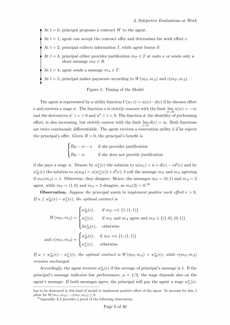
• At t = 0, principal proposes a contract W to the agent.

• At t = 1, agent can accept the contract offer and determines his work effort e.

• At t = 2, principal collects information I, while agent learns S.

• At t = 3, principal either provides justification mP ∈ I at costs κ or sends only ashort message mP ∈ R.

• At t = 4, agent sends a message mA ∈ T .

• At t = 5, principal makes payments according to W (mP ,mA) and c(mP ,mA).?

Figure 1: Timing of the Model

The agent is represented by a utility function U(w, e) = u(w)−d(e) if he chooses effort

e and receives a wage w. The function u is strictly concave with the limit limw→0

u(w) = −∞and the derivatives u′ > ε > 0 and u′′ < ε < 0. The function d, the disutility of performing

effort, is also increasing, but strictly convex with the limit lime→1

d(e) =∞. Both functions

are twice continously differentiable. The agent receives a reservation utility u if he rejects

the principal’s offer. Given B > 0, the principal’s benefit isBµ− w − κ if she provides justification

Bµ− w if she does not provide justification

if she pays a wage w. Denote by w∗L(e) the solution to u(wL) = u+ d(e)− ed′(e) and by

w∗H(e) the solution to u(wH) = u(w∗L(e)) + d′(e). I call the message mP and mA agreeing

if mP (mA) = 1. Otherwise, they disagree. Hence, the messages mP = (0, 1) and mA = 2

agree, while mP = (1, 0) and mA = 2 disagree, as mP (2) = 0.10

Observation. Suppose the principal wants to implement positive work effort e > 0.

If κ ≤ w∗H(e)− w∗L(e), the optimal contract is

W (mP ,mA) =

w∗H(e), if mP =∈ {1, (1, 1)}

w∗L(e), if mP and mA agree and mP ∈ {(1, 0), (0, 1)}

2w∗H(e), otherwise

and c(mP ,mA) =

w∗H(e), if mP =∈ {1, (1, 1)}

w∗L(e), otherwise.

If κ > w∗H(e) − w∗L(e), the optimal contract is W (mP ,mA) = w∗H(e), while c(mP ,mA)

remains unchanged.

Accordingly, the agent receives w∗H(e) if the average of principal’s message is 1. If the

principal’s message indicates low performance, µ = 1/2, the wage depends also on the

agent’s message. If both messages agree, the principal will pay the agent a wage w∗L(e).

has to be destroyed in this kind of model to implement positive effort of the agent. To account for this, Iallow for W (mP ,mA)− c(mP ,mA) ≥ 0.

10Appendix A.5 provides a proof of the following observation.

Page 8 of 40

3. Justify Bad Evaluations

If the messages disagree, the agent receives w∗L(e) while the principal has to pay 2w∗H(e).

For small κ, this contract yields a number of observations that are confirmed by

the results in the next sections. First, there is truth-telling although the agent does

not know the correct evaluation. Second, the principal justifies only bad evaluations,

µ = 1/2. Third, the agent’s wage does not depend on his message. Fourth, the agent

understands a justification, i.e., he learns the result of the evaluation and can partially

verify the message. Furthermore, on the equilibrium path, there are no payments to third

parties. To understand these features, consider the principal’s incentives if she has learned

I = (1, 1). If she does not provide justification, her payoff is B−w∗H(e) for a high message

or B−2w∗H(e) for a low message. If she provides justification, her payoff is B−w∗H(e)−κfor a high message or B−w∗L(e)/2−w∗H(e)−κ for a low message as she expects the agent

learn S = 1 or 2 with probability 1/2 each. Hence, it is optimal for the principal to report

truthfully and not to justify the evaluation in this case. If she has learned I = (1, 0) or

(0, 1), her payoff without justification is B/2−w∗H(e) for a high message or B/2−2w∗H(e)

for a low message. If she provides justification and sends a truthful message, her payoff is

B/2−w∗L(e)−κ. The other cases are analogous. Therefore it is optimal for the principal

to report truthfully and to justify the evaluation in this case. Yet the stylized nature of

the example makes it impossible to study communication patterns in more detail. For

this purpose, the next section generalizes the model making the evaluation continuous

and reducing the fraction of sources that the agent learns to 0.

3 Justify Bad Evaluations

3.1 The Main Model

This time, the principal proposes a contract W that specifies the agent’s wage depending

on any information that is available at the time of the wage payments and enforceable by

a third party. After the agent’s effort choice e ∈ [0, 1), the principal collects subjective

information I(t) ∈ {0, 1} about the agent’s work from different sources or performance

areas t ∈ T = [0, 1]. Every source t ∈ T is independent and identically distributed and

declares success with probability p and failure with probability 1− p. The probability p

is once drawn from the distribution F (p|e) = eFH(p) + (1 − e)FL(p) and therefore de-

pends on the agent’s effort e. The cumulative distribution functions FH(p) and FL(p)

admit continuous densities fH(p), fL(p) > ε > 0. In addition, the distribution F of p

satisfies the monotone likelihood ratio property, i.e., the ratio fH(p)/fL(p) is strictly in-

creasing in p. Notice that the evaluation µ is a sufficient statistics for the agent’s effort,

as µ =∫T I(t)dt = p.11 The monotone likelihood ratio property ensures that a higher

evaluation µ indicates higher work effort.

11I assume a law of large number here. Judd (1985) constructs a probability measure that allows avoidingmeasurability problems in formulating a law of large numbers for a continuum of random variables. Sun(2006) proves such a law of large numbers assuming essential pairwise independence.

Page 9 of 40

3. Justify Bad Evaluations

The agent observes only the reports of a finite subset S ⊂ {t ∈ T |I(t) = 1} of

positive sources with |S| = n. In Section 6 the agent also learns the reports of sources

that report 0. This assumption does not change the results. It is important, however,

that the agent does not learn anything about the subjective evaluation µ. Assume that

the agent’s sample S is large and consists of a random draw with full support over the

positive sources, no atoms and a density bounded away from zero.12 The set S is private

information of the agent, while n is common knowledge. Hence, the principal does not

know which information is observed by the agent. For later reference, denote by P (S|I, e)the conditional distribution and by P (I, S|e) the joint distribution of the agent’s sample S

and the principal’s information I: t 7→ I(t) conditional on the agent’s effort e.

Let β ∈ {0, 1} denote the principal’s justification decision. For β = 0, she does

not provide justification and her message space is restricted to R = [0, 1]. For β = 1,

the principal justifies her evaluation of the agent’s work at cost κ by sending a message

mP ∈ I = {0, 1}T .13 The agent replies with a cheap-talk message mA ∈ Tn. Finally,

the contract W is performed according to the available and enforceable information, the

messages mP and mA. Therefore, the contract is a function W : I × Tn → R+. The

message spaces are sufficiently rich to encode β, e and µ. Thus, it is unnecessary to

include them explicitly in the contract. The principal has no commitment power other

than the contract.

3.2 Analysis

It is crucial here that the principal has to pay communication costs κ to transmit the

information I. The model ensures this by making it impossible to encode the information I

in a message from the restricted message set R. The reason is that the cardinality of I and

R differs. Due to the restriction of the message space for β = 0, the classical revelation

principle does not apply. See Green and Laffont (1986) for an example. Hence, it is

unclear whether truthful revelation is optimal in my setting. Define truthful revelation

by the principal as

θ(I, β) =

I if β = 1∫T I(t)dt if β = 0.

Lemma 3 in the appendix proves that truthful revelation is optimal if an optimal contract

exists. Thus, in the optimal contract principal and agent send a truthful message that

reveals their private information, the principal’s information I or its average µ and the

agent’s sample S respectively.14 Grossman and Hart (1983) prove that the model can

12All results are such that ∃N ∈ N and the results are valid for all n > N. If n is small, e.g., n = 1, theresults also hold, but require higher off-equilibrium payments.

13{0, 1}T denotes the set of all functions T → {0, 1}. For β = 0, I identify a message mP ∈ R in therestricted message space R = [0, 1] with the step function: T → {0, 1} with 1 for t ≤ mp and 0 otherwise.

14Yet it is impossible to have the agent reveal his work effort e truthfully and make the wage dependenton his message about the effort in order to implement e > 0. Therefore it is without loss of generality for

Page 10 of 40

3. Justify Bad Evaluations

be solved in two steps. First, for every level of effort e, the optimal contract W and

its expected costs C(e) for the principal are computed. The second step determines the

optimal effort level e by

maxe∈[0,1)

B

∫pdF (p|e)− C(e).

Now, returning to the first step, Program A below determines the optimal contract that

implements effort e by choosing payments W (mP ,mA) for the principal, c(mP ,mA) for

the agent, and which evaluations to justify, β(I). The objective is to minimize the ex-

pected wage payment subject to several conditions. The participation constraint (PC)

makes the agent willing to accept the proposed contract. The agent’s incentive compati-

bility (ICA) guarantees that the agent chooses the desired level of effort. The principal’s

incentive compatibility (ICP ) gives her an incentive to justify her evaluation if justifica-

tion is desired. In addition, sending a truthful message has to be incentive compatible

for the principal (ICP ) and the agent (ICmA). Finally, the principal’s payment has to

be higher than the wage received by the agent. To simplify the exposition, define the

equilibrium payments Weq(I, S) = W(θ(I, β(I)), S

)and ceq(I, S) = c

(θ(I, β(I)), S

).

C(e) = inf

∫Weq(I, S) + κβ(I)dP (I, S|e), (A)

subject to

∫u(ceq(I, S)

)dP (I, S|e)− d(e) ≥ u, (PC)

e ∈ arg max

∫u(ceq(I, S)

)dP (I, S|e)− d(e), (ICA)

κβ(I) +

∫Weq(I, S)dP (S|I, e) ≤ κ+

∫W (I , S)dP (S|I, e)

∀I ∈ I,∀(κ, I) ∈{{0} ×R, {κ} × I

}, (ICP )∫

u(ceq(I, S))dP (I|S, e) ≥∫u(ceq(I, S))dP (I|S, e) ∀S, S ∈ Tn, (ICmA)

W (I, S) ≥ c(I, S) ∀I ∈ I,∀S ∈ Tn. (1)

If the principal’s information I were observable and contractible, the principal’s and

the agent’s incentive for sending truthful messages (ICP ) and (ICmA) can be neglected.

Denote this problem by A∗, the solution, the optimal complete wage, by w∗e(µ), and the

expected costs by C∗(e).

Lemma 1. If the principal’s information I is contractible, the optimal wage w∗e(µ) de-

pends only on the average µ of the principal’s information I. w∗e(µ) is almost surely

continuous and increasing in µ for positive effort, e > 0.

The results of Holmstrom (1979) remain valid in this setting: The wage depends only

on the sufficient statistics µ instead of the entire information I and a better evaluation

implies a higher wage.

the messages to contain only the information the contracting parties collected at t = 2.

Page 11 of 40

3. Justify Bad Evaluations

If the principal’s information is subjective and justification is a choice variable of

the principal, the additional incentive constraints for the messages do matter. Yet these

incentive constraints do not change the equilibrium wage in the absence of communication

costs when κ = 0.

Lemma 2. If communication costs are κ = 0, all evaluations are justified.

The optimal contract is

c+(mP ,mA) = w∗e

(∫mP (t)dt

)

W+(mP ,mA) =

w∗e

(∫mP (t)dt

)if mP (t) = 1 for all t ∈ mA

2w∗e (1) otherwise.

The equilibrium wage is w∗e(µ), the same as in Lemma 1. Whenever communication is

costly and κ > 0, however, the equilibrium wage differs from w∗e(µ). To gain some intu-

ition, suppose for the moment that the principal justifies all evaluations. Then the optimal

contract implements wage payments w∗e(µ) on the equilibrium path as in Lemma 2. Yet,

the principal can modify this contract to save on communication costs. The reason is that

the agent does not suspect a distorted evaluation by the principal and does not demand

an explanation for the highest wages. Therefore it is suboptimal to justify all evaluations.

For ease of exposition, denote the justification set by IC = {I ∈ I|β(I) = 1}.

Proposition 1. If κ > 0, justifying all evaluations is not optimal, i.e., Pr(IC) < 1.

The proof in the appendix shows that the principal’s total costs decrease if the princi-

pal refrains from justifying evaluations that yield the highest wages. To further determine

the justification set, it is necessary to know more about the optimal contract. The next

proposition provides a solution to Program A and characterizes the optimal contract.

Proposition 2. Suppose Pr(IC) > 0. Then optimal wages are constant for evaluations

outside the justification set. Otherwise, wages depend on the average of the principal’s

evaluation if the messages agree.

c∗∗(mP ,mA) =

w∗∗

(∫mP (t)dt

)if mP ∈ IC

w∗∗ if mP /∈ IC

W ∗∗(mP ,mA) =

w∗∗

(∫mP (t)dt

)if mP ∈ IC and mP (t) = 1 for all t ∈ mA

w∗∗ if mP /∈ IC

w∗∗ + κ otherwise.

The principal justifies low payments, as w∗∗(∫mP (t)dt

)≤ w∗∗ − κ for all mP ∈ IC .

There is pooling of wages, but evaluations are unbiased in the optimal contract. Yet,

this is for ease of exposition only. It is easy to introduce also pooling of evaluations

Page 12 of 40

3. Justify Bad Evaluations

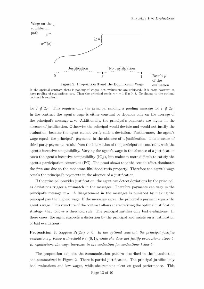
Wage on theequilibriumpath

Result µof theevaluation

w∗∗

w∗∗(δ)

δ0 1

≥ κ{

Justification No Justification

Figure 2: Proposition 3 and the Equilibrium Wage

In the optimal contract there is pooling of wages, but evaluations are unbiased. It is easy, however, tohave pooling of evaluations, too. Then the principal sends mP = 1 if µ ≥ δ. No change to the optimalcontract is required.

for I /∈ IC . This requires only the principal sending a pooling message for I /∈ IC .

In the contract the agent’s wage is either constant or depends only on the average of

the principal’s message mP . Additionally, the principal’s payments are higher in the

absence of justification. Otherwise the principal would deviate and would not justify the

evaluation, because the agent cannot verify such a deviation. Furthermore, the agent’s

wage equals the principal’s payments in the absence of a justification. This absence of

third-party payments results from the interaction of the participation constraint with the

agent’s incentive compatibility. Varying the agent’s wage in the absence of a justification

eases the agent’s incentive compatibility (ICA), but makes it more difficult to satisfy the

agent’s participation constraint (PC). The proof shows that the second effect dominates

the first one due to the monotone likelihood ratio property. Therefore the agent’s wage

equals the principal’s payments in the absence of a justification.

If the principal provides justification, the agent can detect deviations by the principal,

as deviations trigger a mismatch in the messages. Therefore payments can vary in the

principal’s message mP . A disagreement in the messages is punished by making the

principal pay the highest wage. If the messages agree, the principal’s payment equals the

agent’s wage. This structure of the contract allows characterizing the optimal justification

strategy, that follows a threshold rule. The principal justifies only bad evaluations. In

these cases, the agent suspects a distortion by the principal and insists on a justification

of bad evaluations.

Proposition 3. Suppose Pr(IC) > 0. In the optimal contract, the principal justifies

evaluations µ below a threshold δ ∈ (0, 1), while she does not justify evaluations above δ.

In equilibrium, the wage increases in the evaluation for evaluations below δ.

The proposition exhibits the communication pattern described in the introduction

and summarized in Figure 2. There is partial justification. The principal justifies only

bad evaluations and low wages, while she remains silent on good performance. This

Page 13 of 40

3. Justify Bad Evaluations

confirms empirical observations, like the leniency bias and the centrality bias that there is

less distinction in subjective evaluations than in the underlying performance measure, in

particular at the top. Yet this behavior is not the result of a bias, but part of the optimal

contract, which pools several evaluations and rewards them with the same wage. Thus,

the contract eliminates wage differences that the principal would have to justify.

The proof is by contradiction. Assume there is a threshold µ∗ such that the principal

justifies some evaluations above µ∗, but does not provide justification for some evalua-

tions below µ∗. This communication pattern implies a constant wage for the evaluations

above µ∗ in the justification set. To show this, the proof establishes that the Lagrange

multiplier of the modified principal’s incentive compatibility (ICP ) is positive on this set

of evaluations.

The second step splits the set of the evaluations above µ∗ in the justification set

into a lower and an upper half. Then the contract is adjusted so that the principal

justifies evaluations in the lower half, but not in the upper half. At the same time the

agent’s wage is decreased in the lower half and increased in the upper half such that

the agent’s expected utility remains constant. Hence, the agent’s participation constraint

(PC) remains satisfied. Finally, I show that the agent’s incentive compatibility (ICA)

becomes slack by this contract modification due to the monotone likelihood ratio property.

Yet, in this case the initial contract cannot be optimal.

Proposition 2 characterized the optimal contract. It remains to determine the values

of w∗∗ and w∗∗(µ).

Proposition 4. Suppose δ > 0. The wages w∗∗ and w∗∗(µ) for µ ∈ [0, δ] are determined

byinf

w(µ),w,δ

∫ δ

0w(µ) + κdF (µ|e) + (1− F (δ|e))w, (D)

subject to

∫ δ

0u(w(µ)

)dF (µ|e) + (1− F (δ|e))u(w)− d(e) ≥ u, (PC)∫ δ

0u(w(µ)

)(fH(µ)− fL(µ))dµ+ u(w)

∫ 1

δfH(µ)− fL(µ)dµ = d′(e) (ICA)

Justification is indeed optimal if communication costs are not prohibitively high as

specified in the next proposition. Then the optimal contract makes the principal justify

some evaluations.

Proposition 5. In the optimal contract, justification occurs with positive probability,

Pr(IC) > 0, if the principal wants to implement positive effort e > 0 and the communi-

cation costs are not too high,

κ ≤ u−1

(u+ d(e) +

f(0|e)fL(0)− fH(0)

d′(e)

)−∫w∗e (p) dF (p|e). (2)

Justification is beneficial, although it is costly and conveys no additional information

about the agent’s effort. Justification also does not provide the principal with information

Page 14 of 40

4. Stochastic Contracts

for her decision making nor gives the agent instructions in the sense of learning or which

tasks to perform. Instead, justification makes the principal’s promise of incentives to

the agent credible and allows the principal to assure the agent that her evaluation is not

distorted. Thus, it is in the principal’s interest to be transparent about her evaluations,

even if justification is costly and takes place after the agent’s effort choice. Next, consider

the optimal amount of justification.

Proposition 6. For e > 0, the justification threshold δ is determined by

u(w∗∗)− u(w∗∗(δ)) = u′(w∗∗(δ))(w∗∗ − w∗∗(δ)− κ).

For small communication costs, the contract converges to complete justification and to

the optimal complete contract from Lemma 1: δ ↗ 1 for κ ↘ 0. No justifications are

provided for large communication costs, κ > u−1(u+ d(e) + f(0|e)

fL(0)−fH(0)d′(e)

).

Finally, consider two extensions to simplify the contract and make it ex-post budget

balanced.

4 Stochastic Contracts

For stochastic payments, the expected value for the principal is higher than the agent’s

certainty equivalent. Therefore it is possible to replace payments to a third party by

stochastic payments. This does not require a risk-neutral principal. As long as the degree

of risk aversion differs between the principal and the agent, the optimal contract can

achieve ex-post budget balance.

Proposition 7. Stochastic contracts allow making the optimal contract ex-post budget-

balanced:

W ∗∗(mP ,mA) =

w∗∗(

∫mP (t)dt) if mP ∈ IC and mP (t) = 1 for all t ∈ mA

w∗∗ if mP /∈ IC

w∗∗ + Λz(∫mP (t)dt) otherwise.

The lotteries Λz have E(Λz) = κ and a certainty equivalent for the agent of w∗∗(µ) =

u−1(E[u(w∗∗ + Λz(µ))]). The values of w∗∗ and w∗∗(µ) are determined in Proposition 4.

Stochastic contracts ensure ex-post budget balance. Examples are stock options whose

valuation is influenced by external shocks to the financial sector or uncertain arbitration

procedures. The contracting parties might be uncertain how a disagreement is interpreted

and which wage payment is appropriate.

Page 15 of 40

6. Robustness of the Results

5 Indirect Mechanism

The contract described in Proposition 2 can be simplified by changing the agent’s re-

porting strategy. Hence, reduce his messages to the binary decision whether to accept or

reject the evaluation by the principal. If he accepts the evaluation µ, the principal pays

him the corresponding wage w∗∗(µ). If he rejects, the principal has to pay w∗∗+ κ, while

the agent receives w∗∗(µ). Thus, the agent has the possibility to object to the principal’s

evaluation. This conflict resolution might be quite realistic, as Bretz et al. (1992, p. 332)

state that “most organizations report having an informal dispute resolution system (e.g.,

open door policies) that employees may use to contest the appraisal outcome. About one-

quarter report having formalized processes.” At the same time, change the principal’s

reporting strategy: If the evaluation µ is above the threshold δ, send message mP = 1.

Otherwise, justify the truth, i.e., send message mP = I.

The indirect mechanism leaves the incentives of the contracting parties unchanged. If

the principal receives information in the justification set, any deviation makes her worse

off, as the deviation increases her payments to at least w∗∗. For evaluations outside the

justification set, it is also unprofitable to deviate, as any evaluation yielding a lower

wage will be rejected. For the agent, on the other hand, the following strategy is a best

reply: accept an evaluation if and only if the principal proposed µ ≥ δ or she provides

justification that matches the agent’s information. Consequently, the modified setting

also implements effort e of the agent at optimal costs. Hence, the relevant part of the

model is the principal’s decision to justify her evaluation to the agent at t = 3.

6 Robustness of the Results

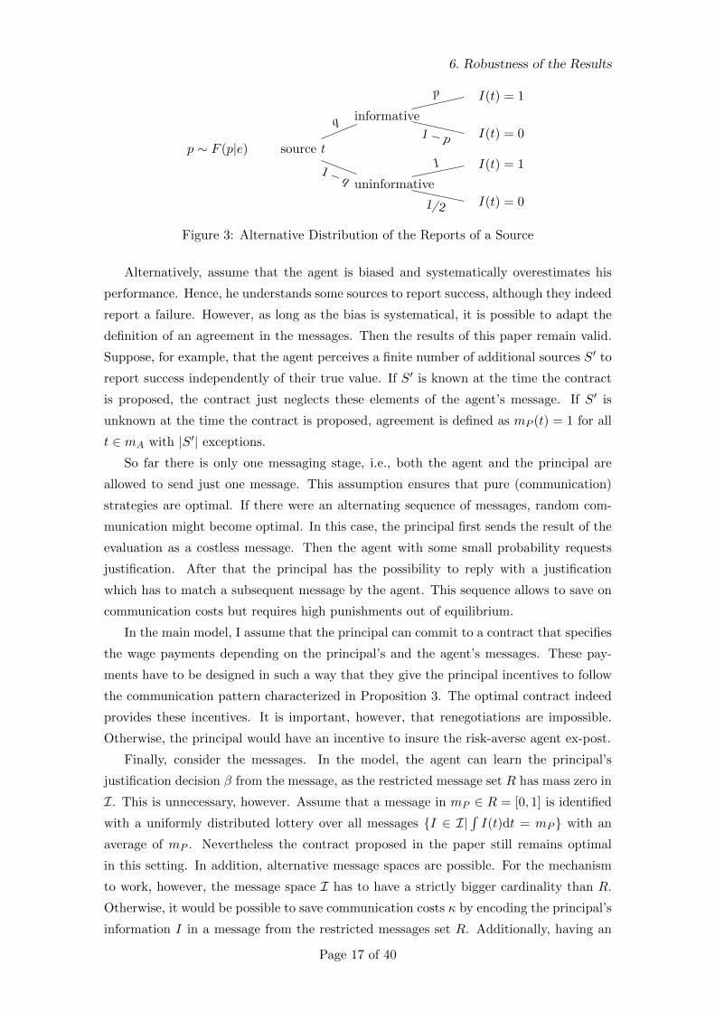
In the model, the agent learns the reports of a finite subset S of positive signals. It is

possible, however, to extent the model to include negative signals into S. For this purpose

assume, that there are informative and uninformative sources. A source is informative

with probability 1 > q > 0. In this case, the source reports a success with probability p

as before. With probability 1−q the source is uninformative and reports statistical noise,

i.e., success or failure with probability 1/2 each. The quality of a source is unobservable.

Figure 3 depicts the distribution for each source. The set S is drawn randomly from the

uninformative sources. Then the agent learnsI(t) if t ∈ S

0 if t /∈ S.

In this case my results remain valid even if S is unobservable by the agent. There are

some adaptations to the optimal contract in this case. In particular, the consensus wage

is paid, if the messages agree, i.e., mP (t)mA(t) = mA(t) for all t ∈ T .

Page 16 of 40

6. Robustness of the Results

p ∼ F (p|e) source t

uninformative

I(t) = 01/2

I(t) = 111− q

informative

I(t) = 01− p

I(t) = 1p

q

Figure 3: Alternative Distribution of the Reports of a Source

Alternatively, assume that the agent is biased and systematically overestimates his

performance. Hence, he understands some sources to report success, although they indeed

report a failure. However, as long as the bias is systematical, it is possible to adapt the

definition of an agreement in the messages. Then the results of this paper remain valid.

Suppose, for example, that the agent perceives a finite number of additional sources S′ to

report success independently of their true value. If S′ is known at the time the contract

is proposed, the contract just neglects these elements of the agent’s message. If S′ is

unknown at the time the contract is proposed, agreement is defined as mP (t) = 1 for all

t ∈ mA with |S′| exceptions.

So far there is only one messaging stage, i.e., both the agent and the principal are

allowed to send just one message. This assumption ensures that pure (communication)

strategies are optimal. If there were an alternating sequence of messages, random com-

munication might become optimal. In this case, the principal first sends the result of the

evaluation as a costless message. Then the agent with some small probability requests

justification. After that the principal has the possibility to reply with a justification

which has to match a subsequent message by the agent. This sequence allows to save on

communication costs but requires high punishments out of equilibrium.

In the main model, I assume that the principal can commit to a contract that specifies

the wage payments depending on the principal’s and the agent’s messages. These pay-

ments have to be designed in such a way that they give the principal incentives to follow

the communication pattern characterized in Proposition 3. The optimal contract indeed

provides these incentives. It is important, however, that renegotiations are impossible.

Otherwise, the principal would have an incentive to insure the risk-averse agent ex-post.

Finally, consider the messages. In the model, the agent can learn the principal’s

justification decision β from the message, as the restricted message set R has mass zero in

I. This is unnecessary, however. Assume that a message in mP ∈ R = [0, 1] is identified

with a uniformly distributed lottery over all messages {I ∈ I|∫I(t)dt = mP } with an

average of mP . Nevertheless the contract proposed in the paper still remains optimal

in this setting. In addition, alternative message spaces are possible. For the mechanism

to work, however, the message space I has to have a strictly bigger cardinality than R.

Otherwise, it would be possible to save communication costs κ by encoding the principal’s

information I in a message from the restricted messages set R. Additionally, having an

Page 17 of 40

7. Conclusion

(at least countable) infinite message space R helps to avoid integer problems.

7 Conclusion

This article discusses communicating a subjective performance measure in a principal-

agent model. The principal can justify her evaluation of the agent’s work. Providing

justification is costly, does not convey additional information about the agent’s effort, and

does not serve a learning or instructing purpose. Nevertheless, in the optimal contract the

principal justifies some evaluations. This allows the agent to detect distorted evaluations.

Therefore providing a justification makes the incentives for the agent credible. In the

optimal contract, the principal justifies only bad evaluations. This communication pattern

results in pooling and wage compression at the top, as illustrated in Figure 2 on page 13.

These results fit well with empirical observations, often referred to as leniency bias and

centrality bias.15 The paper argues that this pattern of evaluations is a feature of the

optimal contract with unbiased agents and no proof of biased behavior per se.

The principal’s justification convinces the agent that the principal evaluates her ap-

propriately ex-post. In addition, they motivate him ex-ante to implement the specified

work effort. Compare this to a naive contract that does not give the principal an incentive

to provide justification. In this naive contract, the principal does not justify the evalua-

tion and always reports the evaluation associated with the lowest wage. Anticipating this

behavior the agent is unmotivated to implement any positive work effort. This partially

explains the concern of the management literature to ensure credible feedback provision.

In addition, the problem of credible evaluations provides a partial answer to Fuchs (2007,

p. 1446), who emphasizes the importance of exploring “possible reasons for the existence

of communication” between agents and principals. Communication at the interim stages

might be explained by training and instruction reasons, but credibility problems are re-

sponsible for communication in the last stages of the principal-agent relation.

The results of this paper are important for the design of incentives systems. First, the

systems have to ensure the credible provision of appropriate feedback by institutionalizing

the feedback process or using multi-source feedback. Second, the pooling at the top could

cause the costs of an incentives scheme to be substantial if there is a bonus attached to

receiving a positive evaluation and many employees receive a positive evaluation due to

the compression at the top.16

This paper assumes that the principal incurs costs for communicating with the agent.

I would get similar results if the principal’s costs instead concerned the acquisition of

information. In this case, the principal only learns the result of the evaluation, i.e., the

15“The distribution of ratings is typically both concentrated and biased.” (Gibbs, 1991, p. 5)16Bernardin and Orban (1990, p. 199) provide the example of the Small Business Administration and

NASA introducing a bonus scheme based on subjective evaluations. After more than 50% of eligibleemployees should receive a bonus, Congress responded with the requirement that no more than 25% ofemployees shall receive a bonus.

Page 18 of 40

A. Appendix

average µ =∫I(t)dt of the information I. Then she decides whether to spend κ to

acquire the entire information I. Independently of her choice of information acquisition,

the principal can send a cheap-talk message in the unrestricted message set I. Both

settings have some merits; in reality, there could be a mixture of these two polar cases.

A Appendix

A.1 The Optimal Complete Contract

Lemma 1 characterizes the optimal complete contract and states the solution to Pro-

gram A∗ if the principal’s information I is public and verifiable. This yields a benchmark

solution w∗e(µ), the optimal complete wage. Additionally, the lemma shows that every

effort e ∈ [0, 1) is implementable at finite costs C∗(e).

Proof of Lemma 1: Holmstrom (1979) shows that the optimal wage only conditions

on µ =∫I(t)dt, because the average of the principal’s information I is a sufficient statis-

tics for the agent’s effort, Pr(I, S|e,∫I(t)dt) = Pr(I, S|

∫I(t)dt). In order to implement

no effort, e = 0, set w∗0(µ) = u−1(u+ d(0)) for all µ.

If, on the other hand, the desired effort is positive, e > 0, the agent’s incentive

compatibility matters. The first-order approach is valid here, because F (p|e) is a linear

combination of distribution functions. This implies that the convex distribution function

condition is satisfied. According to Grossman and Hart (1983) and Rogerson (1985),

the convex distribution function condition in combination with the convexity of d(·) and

the monotone likelihood ratio property guarantees that the first-order approach is valid.

Therefore, the agent’s incentive compatibility reads∫u(w(µ))(fH(µ)− fL(µ))dµ = d′(e) (ICA)

In addition, the constraint set is nonempty. Take for example any w > 0 and the contract

w(µ) =

w if fH(µ)− fL(µ) ≥ 0

h(w) otherwise

with h(w) positive, but small enough, such that the agent’s incentive compatibility

(ICA) is satisfied. This implicitly defines an increasing function h(·). Consequently,

there is a w fulfilling the participation constraint (PC) with equality. Therefore the

constraint set of Program A∗ is nonempty. Moreover, the costs of the contract are

h(w)F (ζ|e) + w(1− F (ζ|e)) < w <∞ with ζ = inf{µ ∈ [0, 1]|fH(µ)− fL(µ) ≥ 0}.Holmstrom (1979) proves that the Lagrange multipliers of the participation constraint

λ1 and of the incentive compatibility λ2 are positive. Pointwise optimization17 determines

17This technique allows for piecewise continuous functions, as Kamien and Schwartz (1991) show inPart II, Section 12. Therefore bonus wages are possible and there is no restriction to continuous contracts.

Page 19 of 40

A. Appendix

the optimal contract as

f(µ|e)− λ1u′(w(µ))f(µ|e)− λ2u

′(w(µ))(fH(µ)− fL(µ)) = 0 a.s.,

1

u′(w(µ))= λ1 + λ2

fH(µ)− fL(µ)

f(µ|e)= λ1 + λ2

fH(µ)fL(µ)

− 1

efH(µ)fL(µ)

+ 1− ea.s. (3)

Since the fraction l−1el+1−e is increasing in l, the right-hand side of above equation is in-

creasing in µ due to the monotone likelihood ratio property. Therefore the concavity

of u(·) implies that w∗e(µ) is increasing in µ ∈ [0, 1] almost surely. Moreover, w∗e(µ) is

continuous almost surely and any discontinuity is removable, because the densities fH

and fL are continuous.

A.2 The Optimal Contract

I begin by considering the optimal contract in the absence of communication costs, κ = 0.

Proof of Lemma 2: First, I show that the contract proposed in Lemma 2 satisfies the

additional incentive constraints (ICP ) and (ICmA). As the agent’s wage is independent

of mA, (ICmA) is trivially satisfied. Now consider a deviation by the principal. For this

purpose, consider a subset D ⊂ T with∫D 1dt > 0. Then there is a N ∈ N, such that a

deviation on D is unprofitable for the principal for all n > N , because the probability of

a mismatch in the messages is sufficiently close to 1. Additionally, deviations on larger

subsets of T are also unprofitable given the assumption of full support and no atoms

for the distribution of the agent’s sample S. What about deviating on a subset D with

infinitesimal mass∫D 1dt? Consider a parameterization of such deviations D(v), which

maps [0, 1] to the Borel algebra on T , with v =∫D(v) 1dt. In the limit for v → 0 the

potential gain of a deviation and the probability of detection converge to 0. Yet, for

v → 0 such a deviation is unprofitable if

∂w∗e(µ)

∂µ< w∗e(1)

∂Pr(S ∩D(v) 6= ∅|I, e)∂v

(0)

for all µ ∈ [0, 1]. The left-hand side of this inequality captures the potential gain of a

deviation and is determined by Eq. (3). The right-hand side of this inequality equals the

penalty w∗e(1) multiplied with the density of at least one source from the agent’s sample

being an element of D(0). This density is increasing in the size n of the agent’s sample.

Therefore there is a N ∈ N, such that a deviation on D is unprofitable for the principal

for all n > N . Hence, the additional incentive constraints (ICP ) and (ICmA) are satisfied.

Second, the contract proposed in Lemma 2 is the optimal contract, because it satisfies

the additional incentive constraints (ICP ) and (ICmA) and implements the equilibrium

wage w∗e(µ). As w∗e(µ) is a solution to Problem A∗ according to Lemma 1, we have found

a solution to Problem A for κ = 0.

Page 20 of 40

A. Appendix

According to Proposition 1, it is suboptimal to provide justification almost surely.

Proof of Proposition 1: Suppose the principal justifies almost surely, i.e., Pr(IC) =

1. Then the expected communication costs are κE(β(I)) = κ and it just remains to

minimize the wage costs. Yet it is possible to implement payments w∗e(µ) defined in

Program A∗ by the following contract.

W (mP ,mA) =

w∗e(µ)

if mP (t) = 1 for all t ∈ mA

w∗e(1) + 2κ if mP (t) 6= 1 for some t ∈ mA

and c(mP ,mA) = w∗e(µ) with µ =∫mP (t)dt. For the same reasons as in the proof of

Lemma 2, the additional incentive constraints (ICP ) and (ICmA) are satisfied. Further-

more, the equilibrium wage is w∗e(µ), as the parties’ messages agree in equilibrium.

It is possible, however, to implement a certain work effort e of the agent even cheaper

by partial justification. For this purpose, modify the contract W to

W ′(mP ,mA) =

w∗e( ∫

mP (t)dt)

if mP (t) = 1 for all t ∈ mA

w∗e(1) + 2κ if∫mP (t)dt < δ and mP (t) 6= 1 for some t ∈ mA

w∗e(δ) + κ if∫mP (t)dt ≥ δ and mP (t) 6= 1 for some t ∈ mA

with a δ < 1, such that

fH (δ)− fL (δ) ≥ 0 and w∗e(δ) + κ ≥ w∗e(1). (4)

Lemma 1 proves that w∗e(µ) is almost surely continuous and any discontinuity is remov-

able. Consequently, there exists a continuous function that almost surely equals w∗e(µ).

Replacing w∗e(µ) by that function in the definition of W ′ also yields a solution to Pro-

gram A. This procedure guarantees that the conditions (4) on δ are feasible.

In the contract W ′, for n > N , the principal justifies all evaluations except the highest

ones and the justification set is

IC =

{I ∈ I

∣∣∣∣∫ I(t)dt ≤ δ}.

If the principal’s information indicates a very good performance, µ > δ, justification

would increase her total costs consisting of wage and communication costs as according

to Lemma 1 w∗e(·) is increasing and, hence, w∗e(δ) + κ < w∗e(µ) + κ. In addition, the

conditions in (4) guarantee that constraints (PC) and (ICA) are still satisfied by choosing

the agent’s wage appropriately. Therefore contract W ′ implements effort e of the agent

and is cheaper than the contract W . This shows that the principal will not justify all

evaluations.

Lemma 3 shows that I can concentrate on truthful messages without loss of generality.

Page 21 of 40

A. Appendix

Lemma 3. For every contract W there is a contract W ′, such that

• W ′ gives the agent incentives to implement the same effort e as in W ,

• W ′ has (weakly) lower costs for the principal than W and

• W ′ gives the agent and the principal incentives to send truthful messages.

In addition, contract W ′ has the following structure

c′(mP ,mA) =

c(mP ) if mP ∈ I ′Cw if mP /∈ I ′C

(5)

W ′(mP ,mA) =

w(mP ) if mP ∈ I ′C and mP (t) = 1 for all t ∈ mA

w + κ if mP ∈ I ′C and mP (t) 6= 1 for some t ∈ mA

w if mP /∈ I ′C

(6)

with the justification set I ′C = {I ∈ I|β′(I) = 1}.

Proof: The proof consists of four parts. The first part characterizes the equilibrium

utilities in contract W. In the second part, the contract W ′ is determined in such a way

that the parties have an incentive to send truthful messages. The third part analyzes the

agent’s incentive compatibility (ICA). The fourth part ensures that the new contract W ′

satisfies the agent’s incentive compatibility and participation constraint.

Step 1 Denote the expected payment conditional on information I given equilib-

rium strategies in contract W by w(I) for the principal and the corresponding certainty

equivalent by c(I) for the agent. If in contract W the principal provides no justification

in equilibrium, I /∈ IC , the agent cannot verify the evaluation. The reason is that the

cardinality of I and R differ. According to Cantor’s theorem, the set of all subsets of

a set A has a strictly greater cardinality than the set A itself. Here, the cardinality of

{0, 1}T equals the cardinality of the power set of T and is bigger than the cardinality of

T and the one of R. Hence, it is impossible to encode the information I into a message

in R. No matter which information the principal tells in her message mP ∈ R, the prob-

ability that it matches the agent’s information S is 0. Consequently, the agent cannot

verify the principal’s message. Therefore the principal’s payments have to be constant or

w(I) = w(I ′) for all I, I ′ /∈ IC . Moreover, they have to be higher than the principal’s

payments in the justification set including communication costs.

w(I) ≥ κ+ supI′∈IC

w(I ′) ∀I /∈ IC

Otherwise, the principal would not provide justification and act as if I /∈ IC , because the

agent could not observe this deviation.

Step 2 Consider the contract W ′ given by equations (5) and (6) with I ′C = IC \ Rand w = w(I) for an I /∈ IC .18 The agent’s wage does not depend on his message.

18This requires identifing a message mP ∈ R with the step function: T → {0, 1} with 1 for t ≤ mp and0 otherwise. Additionally, if IC = I, set w = κ+ supI∈IC w(I).

Page 22 of 40

A. Appendix

Therefore he is indifferent between sending any message and the incentive compatibility

for his message is satisfied. If the principal should justify, I ∈ IC , any disagreement in

the messages shows a deviation by the principal and the payment W ′(I, S) with I ∈ ICand I(t) 6= 1 for some t ∈ S matters only for the right-hand side of the principal’s

incentive compatibility (ICP ). Therefore I can increase this payment to satisfy (ICP )

without affecting any other constraint or the objective function. Accordingly, there will

be a penalty for I ∈ IC and I(t) 6= 1 for some t ∈ S. By setting the principal’s payment

in this case to

W (I, S) = w + κ

there is a N ∈ N such that for n > N the principal will never deviate to another message in

the justification set IC . The reason is that a deviation at least weakly increases payments

as

w + κ >

∫W ′(I , S)dP (S|I, e) ≥ w > w(I) =

∫W ′(I, S)dP (S|I, e)

for all I, I ∈ IC with∫{t∈T |I(t)6=I(t)} 1dt > 0. The reasoning is the same as in the proof

of Proposition 1. For large deviations the probability of a mismatch in the messages is

sufficiently close to 1. For small deviations increasing the number of sources in the agent’s

sample increases the density of one of these sources being in the deviation set. On the

margin, the density matters and not the probability. Hence, a deviation is unprofitable.

Step 3 Denote by M(µ) = {I ∈ I|∫I(t)dt = µ} the set of all information with an

average µ. For the agent’s incentives only the expected wage in M(µ) matters, because

the agent’s information, S, does not depend on her effort choice and the average of the

principal’s information is a sufficient statistics for the agent’s effort, Pr(I, S|e,∫I(t)dt) =

Pr(I, S|∫I(t)dt). In addition, Lemma 1 shows that the first-order approach is valid here.

Therefore, the agent’s incentive compatibility (ICA) equals∫ (∫u(c(I))dP (I, S |e, I ∈M(µ))

)(fH(µ)− fL(µ))dµ = d′(e) (7)

Consequently, the agent’s incentives remain unchanged if∫u(c(I))dP (I, S|e, I ∈M(µ)) =

∫u(c′(θ(I, β(I)), S)

)dP (I, S|e, I ∈M(µ)) (8)

for all µ ∈ [0, 1]. By the definition of c′ in (5), the right-hand side equals∫β′(I)u

(c(I)

)dP (I, S|e, I ∈M(µ)) + u(w)

∫1− β′(I)dP (I, S|e, I ∈M(µ))

Hence, the equality in (8) is not guaranteed for all µ, as c(I) ≤ c′(I,mA) = w for I /∈ I ′C .

Step 4 If (8) is not satisfied, it is necessary to reduce the expected wage of the agent.

For this purpose, let the principal justify every evaluation I /∈ IC ∪R with c(I) ≤ w− κ.

Denote the set of these I by I ′. Now set I ′C = I ′C ∪ I ′, c′(I,mA) = c(I) and

Page 23 of 40

A. Appendix

W ′(I,mA) =

c(I) if I(t) = 1 ∀t ∈ mA

w + κ if ∃t ∈ mA : I(t) 6= 1∀I ∈ I ′,∀mA ∈ Tn.

Thus, for any remaining evaluations that are not justified, I /∈ I ′C ∪ R, the agent’s wage

is w − κ < c(I) ≤ w in contract W. Finally, increase the justification set and make the

principal justify a fraction α of the evaluations M(µ) \ I ′C , such that∫u(c(I))dP (I, S |e, I ∈M(µ)) =

∫β′(I)u(c(I))dP (I, S |e, I ∈M(µ)) +

+(αu(w − κ) + (1− α)u(w)

) ∫1− β′(I)dP (I, S |e, I ∈M(µ))

As the agent’s wage is w − κ < c(I) ≤ w for all I /∈ I ′C ∪R, it is possible to find such an

α ∈ [0, 1]. Set α = 1 if α is not uniquely determined, as M(µ) \ I ′C has mass 0. Denote

the addition evaluations that are justified by I ′′. To make justification optimal, adjust

contract W ′ by I ′C = I ′C ∪ (I ′′ \R), c′(I,mA) = w − κ and

W ′(I,mA) =

w − κ if I(t) = 1 ∀t ∈ mA

w + κ if ∃t ∈ mA : I(t) 6= 1∀I ∈ (I ′′ \R),∀mA ∈ Tn.

Repeat these steps for every µ. Then the agent’s incentives in the new contract W ′ are the

same as in contract W. In addition, the agent’s participation constraint is also satisfied

in contract W ′, so that contract W ′ implements effort e at (weakly) lower costs than

contract W.

Lemma 4 proves that contracts in which the agent’s wage payment depends only on

the average of the principal’s information are no loss of generality.

Lemma 4. For every contract W there is a contract W ′ implementing the same effort e at

the same costs as W. Moreover, in contract W ′ the justification choice β and the agent’s

wages just depend on the average of the principal’s information, i.e., β(mP ) = β(m′P ) and

c′(mP ,mA) = c′(m′P ,mA) for all mA ∈ Tn,mP ,m′P ∈ IC with

∫mP (t)dt =

∫m′P (t)dt.

Proof: Lemma 3 shows that the agent’s wage does not depend on his message mA.

In addition, according to equation (7), the agent’s incentive compatibility (ICA) depends

only on the expected utility of the agent given the average of the principal’s information.

The same is valid for the agent’s participation constraint in Program A. Therefore it is

possible without violating these constraints to set c′(mP ,mA) = c (µ) for all mP ∈ ICand mA ∈ Tn with

u (c (µ)) =

∫u(c(I , S)

)dP(I , S

∣∣∣e, I ∈M (µ) ∩ IC), µ =

∫mP (t)dt,

and M(µ) = {I ∈ I|∫I(t)dt = µ}. This reduces at least weakly the expected wage,

Page 24 of 40

A. Appendix

because the agent is risk-averse. Hence,

c (µ) ≤∫c(I , S)dP

(I , S

∣∣∣e, I ∈M (µ) ∩ IC). (9)

Yet, the agent’s new wage c′(mP ,mA) = c(µ) might be higher than the principal’s pay-

ment W (mP ,mA) for some mA and mP ∈ IC . To make the contract feasible and satisfy

constraint (1) in Program A, set

W ′(mP ,mA) =

∫W (I , S)dP

(I , S

∣∣∣e, I ∈M (µ) ∩ IC)

∀mP ∈ IC ,∀mA ∈ Tn

with µ =∫mP (t)dt. This ensures that W ′(mP ,mA) ≥ c(µ) for all mP ,mA, because

W (mP ,mA) ≥ c(mP ,mA) in contract W and the new wage, c(µ), is lower than the

previous expected wage according to equation (9). In addition, the principal’s expected

payments in the new contract W ′ are the same as in contract W, as∫W ′eq(I, S)dP (I, S|e, I ∈M (µ)) =

∫Weq(I, S)dP (I, S|e, I ∈M (µ)) ∀µ.

Consequently, there exists a contract that gives the principal and the agent the same

utility as the old contract W, but makes the agent’s utility depend only on the average

of the principal’s information, i.e., c(mP ,mA) = c(µ) for all mA and all mP ∈ IC . It

remains to ensure constraint (ICP ) in contract W ′. For I ∈ IC in the justification set,

W ′(I, S) with I(t) 6= 1 for some t ∈ S matters only on the right-hand side of constraint

(ICP ). Therefore increasing W ′(I, S) to κ+ supI,SW (I , S) does not affect the objective

function or other constraints, but gives the principal incentives to communicate truthfully.

Additionally, the wage in the justification set is lower than outside this set including the

communication costs, W ′(I, S) + κ < W ′eq(I , S) for all I ∈ IC , I /∈ IC and all S, S ∈ Tn,

because contract W meets this condition according to Lemma 3. This guarantees that

there is a N ∈ N such that for all n > N any deviation in the justification choice, β(I),

and/or the message mP makes the principal worse off. Therefore also the new contract

W ′ satisfies the principal’s incentive compatibility.

It remains to prove that the justification choice does not change within the set M(µ)

for any µ. 1. Suppose there is a µ such that c (µ) ≤ w − κ with w the wage outside the

justification set according to Lemma 3 and c defined by

u (c (µ)) =

∫u(c(I , S)

)dP(I , S

∣∣∣e, I ∈M (µ)).

Then it is possible to justify all I ∈ M(µ) by setting I ′C = I ′C ∪M(µ) and by adapting

the wage as in the first part of the proof.

2. If, on the other hand, c(µ) = w, the principal does not need to provide justification

for all I ∈ M(µ) by setting I ′C = I ′C \ M(µ) and W (I,mA) = c(I,mA) = w for all

Page 25 of 40

A. Appendix

mA ∈ Tn.

3. Finally, in the last case w − κ < c(µ) < w. Denote by A the set of all µ with this

property,

A = {µ ∈ [0, 1]| w − κ < c(µ) < w} .

If the set A has no mass,∫A f(µ|e)dµ = 0, set I ′C = I ′C ∪M(µ) and c(µ) = w − κ for

all µ ∈ A and adapt the wage as in the first part of the proof. If∫A f(µ|e)dµ > 0, there

exists a unique δ, such that justifying only evaluations below δ does not change the agent’s

expected utility, i.e.,∫A

u(c(µ))dF (µ|e) = u(w − κ)

∫A1

dF (µ|e) + u(w)

∫A2

dF (µ|e)

with the sets A1 = {µ ∈ A|µ ≤ δ} and A2 = {µ ∈ A|µ > δ}. For this purpose, modify

the contract to

β′(mP ) =

1 if µ ∈ A1

0 if µ ∈ A2c′(mP ,mA) =

w − κ if µ ∈ A1

w if µ ∈ A2

W ′(mP ,mA) =

w if µ ∈ A2

w − κ if µ ∈ A1 and mP (t) = 1 for all t ∈ mA

w + κ if µ ∈ A1 and mP (t) 6= 1 for some t ∈ mA

for all mP ∈ M(µ), all mA ∈ Tn and all µ ∈ A. As the agent is risk-averse and

W (mP ,mA) ≥ c(mP ,mA) ∈({w} ∪ (0, w − κ]

), this reduces the principal’s payments:∫

A

(∫W (I , S)dP

(I , S

∣∣∣e, I ∈M (µ)))

dF (µ|e) ≥ (w − κ)

∫A1

dF (µ|e) + w

∫A2

dF (µ|e)

In addition, the left-hand side of the agent’s incentive compatibility (7) increases:∫A1

(u(w − κ)− u(c(µ))

)∆f (µ)dµ+

∫A2

(u(w)− u(c(µ))

)∆f (µ)dµ =

=

∫A1

(u(w − κ)− u(c(µ))

)︸ ︷︷ ︸<0

∆f (µ)f(µ|e)f(µ|e)

dµ+

∫A2

(u(w)− u(c(µ))

)︸ ︷︷ ︸>0

∆f (µ)f(µ|e)f(µ|e)

dµ >

>fH(δ)− fL(δ)

f(δ|e)

∫A1

u(w − κ)dF (µ|e) +

∫A2

u(w)dF (µ|e)−∫A

u(c(µ))dF (µ|e)

= 0

with ∆f (µ) = fH(µ)− fL(µ). The monotone likelihood ratio property ensures the strict

inequality and the constant value of the participation constraint yields the final equality.

This shows that the modified contract satisfies the agent’s incentive compatibility (ICA).

Consequently, contract W ′ satisfies all the constraints of Program A and the justifi-

Page 26 of 40

A. Appendix

cation decision just depends on the average of the principal’s information.

Proposition 2 characterizes the optimal contract.

Proof of Proposition 2: Lemma 3 determines the basic structure of the optimal

contract and this proof uses the notation introduced there. Lemma 4 shows that the

justification decision and the agent’s wage just depend on the average of the principal’s

message. It remains to calculate the agent’s wage. First, I prove that there are no

payments to third parties on the equilibrium path. For this purpose, simplify Program A

according to Lemma 3 and 4 to

inf

∫w(I) + κβ(I)dP (I, S|e), (B)

subject to

∫u(c(µ))dF (µ|e)− d(e) ≥ u, (PC)∫u(c(µ))(fH(µ)− fL(µ))dµ = d′(e), (ICA)

w ≥ w(I) + β(I)κ ≥ (1− β(I))w ∀I ∈ I, (ICP )

w(I) ≥ c(∫

I(t)dt

)∀I ∈ I. (10)

(ICP ) ensures that the wage is constant outside the justification set. Furthermore, the

condition requires that the principal’s costs in the justification set, accounting for the

communication costs, is lower than outside this set. According to Lemma 3 this is equiv-

alent to condition (ICP ) in Program A. Condition (10) is the equivalent to (1) in the initial

program and guarantees that payments to third parties are nonnegative. Assume to the

contrary that in the optimal contract there is an I ∈ I, such that w(I) > c(∫I(t)dt

).

Then β(I) = 1, because Lemma 3 and 4 show that c(∫I(t)dt

)= w = w(I) for I /∈ IC . In

addition, it is possible to (weakly) decrease the objective function without violating any

constraint by setting w(I) = c(∫I(t)dt

). Therefore the principal’s consensus payment

just depends on the average of her message and w(I) = c(∫I(t)dt

)for all I ∈ I. This

results in payments to a third party of

W (mP ,mA)− c(∫

mP (t)dt

)=

w − w(mP ) + κ if mP ∈ IC and∃t ∈ S : I(t) 6= 1

0 otherwise.

As the principal’s consensus payments and her justification decision just depend on the

average of the principal’s information, I write them as functions of the average µ instead

of the information I in the following. Finally, it remains to determine the values of w∗∗(µ)

and w∗∗, which solve the following program:

Cc(e) = inf

∫w(µ) + κβ(µ)dF (µ|e), (C)

subject to

∫u(w(µ)

)dF (µ|e)− d(e) ≥ u, (PC)

Page 27 of 40

A. Appendix

∫u(w(µ)

)(fH(µ)− fL(µ))dµ = d′(e), (ICA)

(1− β(µ)) (w(µ)− w) = 0 ∀µ, (11)

w(µ) + κβ(µ) ≤ w ∀µ. (12)

As before, the objective is to minimize the expected costs, here communication costs

and the principal’s payments. The agent’s participation constraint (PC) and incentive

compatibility (ICA) remain unchanged. Constraints (11) and (12) replace condition (ICP ).

Program C determines the optimal contract and completes the proof.

A.3 The Optimal Communication Pattern

Proposition 3 verifies that a threshold strategy is optimal, with justification below a

threshold δ and pooling above δ.

Proof of Proposition 3: Proposition 1 proves that complete feedback is suboptimal

and Pr(IC) < 1. In order to show that only bad evaluations will be justified, assume

to the contrary that in the optimal contract there is a µ∗ with the following properties.

With positive probability the principal justifies evaluations µ above µ∗ and with positive

probability the principal does not justify evaluations µ below µ∗. Denote the correspond-

ing sets by AK = {µ ∈ [0, 1]|µ ≥ µ∗ and β(µ) = 1} for justified evaluations above µ∗ and

evaluations without justification below µ∗ by AN = {µ ∈ [0, 1]|µ ≤ µ∗ and β(µ) = 0}. By

assumption, Pr(AK), Pr(AN ) > 0. Then rewrite program C in the following way. Change

constraint (11) to

f(µ|e) (1− β(µ)) (w(µ)− w)2 ≤ 0 (13)

for all µ. (13) is equivalent to (11), but simplifies the next steps of the proof. This

condition guarantees that the wage is constant outside the justification set, in particular,

in AN . In the justification set and thus in the subset AK , condition (13) is trivially

fulfilled, as 1− β(µ) = 0. Furthermore, multiply constraint (12) by f(µ|e) to obtain

f(µ|e)(w(µ) + κβ(µ)− w) ≤ 0 (14)

for all µ. (14) is equivalent to (12) and guarantees that it is optimal to justify an evaluation

if justification is required by the contract, i.e., β(µ) = 1. Together, both constraints make

justification optimal, if and only if β(µ) = 1. In addition, they ensure that the wage has

to be lower in AK than in AN , as

w(µ)<w=w(µ′) ∀µ ∈ AK , µ′ ∈ AN . (15)

The inequality follows from condition (14), while the equality is given by condition (13).

Define λ1, λ2, ν1(µ) and ν2(µ) to be the Lagrange multipliers of the constraints (PC),

Page 28 of 40

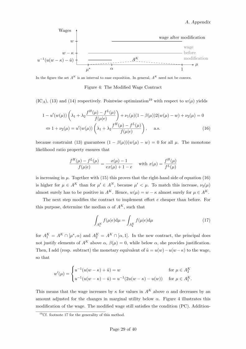
A. Appendix

Wages

µ

wagebeforemodification

wage after modificationw

w − κu−1(u(w − κ)− u)

αµ∗ 1

AK

In the figure the set AK is an interval to ease exposition. In general, AK need not be convex.

Figure 4: The Modified Wage Contract

(ICA), (13) and (14) respectively. Pointwise optimization19 with respect to w(µ) yields

1− u′(w(µ))

(λ1 + λ2

fH(µ)− fL(µ)

f(µ|e)

)+ ν1(µ)(1− β(µ))2(w(µ)− w) + ν2(µ) = 0

⇔ 1 + ν2(µ) = u′(w(µ))

(λ1 + λ2

fH(µ)− fL(µ)

f(µ|e)

), a.s. (16)

because constraint (13) guarantees (1 − β(µ))(w(µ) − w) = 0 for all µ. The monotone

likelihood ratio property ensures that

fH(µ)− fL(µ)

f(µ|e)=

x(µ)− 1

ex(µ) + 1− ewith x(µ) =

fH(µ)

fL(µ)

is increasing in µ. Together with (15) this proves that the right-hand side of equation (16)

is higher for µ ∈ AK than for µ′ ∈ AN , because µ′ < µ. To match this increase, ν2(µ)

almost surely has to be positive in AK . Hence, w(µ) = w − κ almost surely for µ ∈ AK .The next step modifies the contract to implement effort e cheaper than before. For

this purpose, determine the median α of AK , such that∫AK

1

f(µ|e)dµ =

∫AK

2

f(µ|e)dµ (17)

for AK1 = AK ∩ [µ∗, α) and AK2 = AK ∩ [α, 1]. In the new contract, the principal does

not justify elements of AK above α, β(µ) = 0, while below α, she provides justification.

Then, I add (resp. subtract) the monetary equivalent of u = u(w)−u(w−κ) to the wage,

so that

w′(µ) =

u−1(u(w − κ) + u) = w for µ ∈ AK2u−1(u(w − κ)− u) = u−1(2u(w − κ)− u(w)) for µ ∈ AK1 .

This means that the wage increases by κ for values in AK above α and decreases by an

amount adjusted for the changes in marginal utility below α. Figure 4 illustrates this

modification of the wage. The modified wage still satisfies the condition (PC). Addition-

19Cf. footnote 17 for the generality of this method.

Page 29 of 40

A. Appendix

ally, the left-hand side of condition (ICA) is now bigger than the marginal cost of effort,

d′(e), because the left-hand side of condition (ICA) increases by

u

(−∫AK

1

fH(µ)− fL(µ)dµ+

∫AK

2

fH(µ)− fL(µ)dµ

)=

= u

(−∫AK

1

fH(µ)− fL(µ)

f(µ|e)f(µ|e)dµ+

∫AK

2

fH(µ)− fL(µ)

f(µ|e)f(µ|e)dµ

)>

> ufH(α)− fL(α)

f(α|e)

(−∫AK

1

f(µ|e)dµ+

∫AK

2

f(µ|e)dµ

)= 0.

The last equality follows from the definition of α in (17). The main inequality follows

from the increasing likelihood ratio. By reducing the variance of the wage payments until

condition (ICA) holds with equality, condition (PC) becomes slack. This allows decreasing

the wage and shows a contradiction to the existence of µ∗. Therefore the optimal contract

does not require the principal to justify good evaluations, as the agent does not suspect a

distortion of these evaluation results. On the other hand, the principal has to justify bad

evaluations. The set AK can be replaced by any set of justified evaluations and a wage

of w − κ. Thus, in the optimal contract any set with these properties has no mass and,

hence, has no influence on the optimal contract. Therefore, the wage and communication

pattern can be adjusted to a threshold rule with respect to justification. Combining these

results with Program C, allows me to prove analogously to Lemma 1 that w(µ) is strictly

increasing in µ ∈ [0, δ].

Proof of Proposition 4: Consider the relaxed problem:

infw(µ),w,δ

∫ δ

0w(µ) + κdF (µ|e) + (1− F (δ|e))w, (D)

subject to

∫ δ

0u(w(µ)

)dF (µ|e) + (1− F (δ|e))u(w)− d(e) ≥ u, (PC)∫ δ

0u(w(µ)

)(fH(µ)− fL(µ))dµ+ u(w)

∫ 1

δfH(µ)− fL(µ)dµ = d′(e) (ICA)

without constraint (12). The solution to this problem gives the agent the necessary

incentives at minimal costs. Yet this solution might for some µ violate the principal’s

incentive compatibility, namely, w ≥ κ+ w(µ). Nevertheless, I show that the solution to

this problem always satisfies this condition. Therefore the solution to the relaxed problem

is also a solution to the initial program.

Denote the Lagrange multiplier for the participation constraint by λ1 and the one

for the agent’s incentive compatibility by λ2. Then the program yields three first-order

conditions:

f(µ|e)− λ1u′(w(µ))f(µ|e)− λ2u

′(w(µ))(fH(µ)− fL(µ)) = 0 a.s. for µ

(1− F (δ|e))− λ1u′(w)(1− F (δ|e))− λ2u

′(w)

∫ 1

δfH(µ)− fL(µ)dµ = 0

Page 30 of 40

A. Appendix

f(δ|e)(w(δ) + κ− w)− (u(w(δ))− u(w))

(λ1f(δ|e) + λ2(fH(δ)− fL(δ))

)= 0

The last equation ensures w 6= w(δ). Rearranging yields

λ1 + λ2fH(µ)− fL(µ)

f(µ|e)=

1

u′(w(µ))a.s. for µ (18)

λ1 + λ2

∫ 1δ f

H(µ)− fL(µ)dµ

1− F (δ|e)=

1

u′(w)(19)

λ1 + λ2fH(δ)− fL(δ)

f(δ|e)=

w − w(δ)− κu(w)− u(w(δ))

(20)

The monotone likelihood ratio guarantees that

∫ 1

δfH(µ)− fL(µ)dµ

1− F (δ|e)=

∫ 1

δfH(µ)−fL(µ)

f(µ|e) f(µ|e)dµ∫ 1

δf(µ|e)dµ

>

fH(δ)−fL(δ)f(δ|e)

∫ 1

δf(δ|e)dµ∫ 1

δf(δ|e)dµ

=fH(δ)− fL(δ)

f(δ|e).

Additionally, as before, λ1 and λ2 are positive. Then (18) and (19) imply w > w(µ) a.s.

for µ ∈ [0, δ]. Comparing (18) for µ = δ and (20) results in

1

u′(w(δ))=

w − w(δ)− κu(w)− u(w(δ))

(21)

Assume to the contrary that w ≤ w(δ) +κ. Then the left-hand side is non-positive, while

the right-hand side is positive. Therefore w > w(δ) + κ and any solution to the relaxed

problem also satisfies condition (12). Consequently, (18), (19), and (20) in combination

with the participation constraint and the agent’s incentive compatibility determine the

optimal contract.

Proof of Proposition 5: The proof proceeds along the following lines. If e > 0

and the principal justifies almost surely no evaluation, e.g., due to high communication

costs κ, the optimal contract does not exist.20 Yet, for every ε there is a contract whose

costs are at most ε higher than the infimum costs to implement effort e > 0 by the agent.

Finally, the proof shows that condition (2) ensures that the optimal contract provides

justification with positive probability.

In the absence of justification, the principal’s payments have to be constant according

to Lemma 3, as it is impossible to verify her message mP . Denote her payments by w.

The next steps calculate the infimum costs to implement positive effort e > 0 of the

agent. For this purpose, the set of feasible contracts is reduced step by step, as I show

that contracts with specific characteristics are suboptimal. First consider a contract with

c(µ) < w almost surely. In this case, it is possible to reduce the principal’s payments w

without violating any constraint. Therefore I only have to take contracts into account

with a positive probability for {µ ∈ [0, 1]|c(µ) = w}.Second, consider an optimal contract W with a µ∗, such that there are payments to

20There is an optimal contract if the distributions FH and FL have atoms at 0.

Page 31 of 40

A. Appendix

a third party for µ > µ∗ with positive probability, but with positive probability there are

no such payments for µ ≤ µ∗. Denote the corresponding sets by AS = {µ ∈ [0, 1]|µ > µ∗

and c(µ) < w} with third-party payments above µ∗ and the set of evaluations without

such payments below µ∗ by AD = {µ ∈ [0, 1]|µ ≤ µ∗ and c(µ) = w}. By assumption∫AS f(µ|e)dµ,

∫AD f(µ|e)dµ > 0. Now reduce the bigger set, until both sets have the

same mass,∫AS f(µ|e)dµ =

∫AD f(µ|e)dµ. In the next step, I modify the wage to

c′(µ) =

u−1

(1∫

AD f(µ|e)dµ∫AS u(c(µ))f(µ|e)dµ

)for µ ∈ AD

w for µ ∈ AS

c(µ) otherwise.

(22)

On AD the agent’s wage is reduced to the average wage on AS in contract W , while

on AD the wage increases to w. Otherwise, the contract remains unchanged. In order

to check whether this contract is feasible, I analyze the remaining constraints (PC) and

(ICA). By the definition of the wage modification W ′ in (22), the agent’s participation

constraint (PC) is still satisfied. On the other hand, the left-hand side of the agent’s

incentive compatibility (ICA) increases by∫AD

(u(c′(µ))− u(w)

)︸ ︷︷ ︸<0

(fH(µ)− fL(µ))dµ+

∫AS

(u(w)− u(c(µ))

)︸ ︷︷ ︸>0

(fH(µ)− fL(µ))dµ >

>fH(µ∗)− fL(µ∗)

f(µ∗|e)

( ∫AD

u(c′(µ))f(µ|e)dµ−∫AS

u(c(µ))f(µ|e)dµ)

= 0.

The monotone likelihood ratio property ensures the strict inequality and the constant

value of the participation constraint yields the equality. Therefore the modified wage

W ′ in (22) makes the left-hand side of condition (ICA) bigger than the marginal cost of

effort, d′(e). In addition, the contract satisfies condition (PC). By reducing the variance

of the wage payments, until condition (ICA) holds with equality, condition (PC) becomes

slack. This allows decreasing the wage. Consequently, restrict attention to contracts with

a δ < 1, such that c(µ) = w for all µ > δ.

Third, consider such a contract W with δ. To satisfy the agent’s incentive compatibil-

ity, there has to be a payment to a third party, i.e., c(µ) < w, with positive probability.

Denote the corresponding set by AS = {µ ∈ [0, 1]|c(µ) < w} and its median by α. By the

previous remarks, these values are below δ, i.e., µ ≤ δ for all µ ∈ AS . Now, modify the

wage to

c′′(µ) =

u−1(u(µ)) for µ ≤ α and µ ∈ AS

w otherwise

Page 32 of 40

A. Appendix

u(µ) = u(c(µ))− u(w) +2∫

AS f(µ|e)dµ

∫µ∈AS and µ>α

u(c(µ))f(µ|e)dµ.

For evaluations above the median α, the agent’s wage increases to w, while below the

median the wage is reduced to balance the utility gain above the median. Otherwise, the

contract remains unchanged. The proof is now analogous to the last case. Therefore it is

possible to improve the contract, as long as δ > 0. Yet the contract with a constant wage

for the agent and δ = 0 does not satisfy the agent’s incentive compatibility. Therefore an

optimal contract does not exist and I have to consider a sequence of contracts.

For this purpose, construct a sequence of feasible contracts that satisfy the properties

derived in this proof. For those contracts, I derive upper and lower bounds for their costs.

Consider the following contracts for a small δ > 0: Wδ(mP ,mA) = w(δ) and

cδ(mP ,mA) = cδ

(∫mP (t)dt

)=

w(δ) if∫mP (t)dt > δ

w(δ)− Λδ(∫mP (t)dt) if

∫mP (t)dt ≤ δ,

with w(δ) and third-party payments Λδ(µ) such that the agent’s incentive compatibility

and his participation constraint are satisfied. This requires

δ∫0

u(cδ(µ))f(µ|e)dµ+ (1− F (δ|e))u(w(δ)) = u+ d(e) (PC)

δ∫0

u(cδ(µ))(fH(µ)− fL(µ))dµ− u(w(δ))

δ∫0

fH(µ)− fL(µ)dµ = d′(e) (ICA)

as∫ 1δ f

H(µ)−fL(µ)dµ =∫ δ

0 fL(µ)−fH(µ)dµ. The constraint (ICA) implies u(cδ(µ)) < 0

for all µ ≤ δ with δ sufficiently small, because∫ δ

0 fH(µ) − fL(µ)dµ → 0 for δ → 0 and

fH(µ) − fL(µ) < 0 for all µ ≤ δ. Rearranging the agent’s incentive compatibility and

approximating it from above results in

d′(e) ≤ −u(w(δ))

δ∫0

fH(µ)− fL(µ)dµ+fH(0)− fL(0)

f(0|e)

δ∫0

u(cδ(µ))f(µ|e)dµ.

In the next step, insert the participation constraint for∫ δ

0 u(cδ(µ))f(µ|e)dµ to get

u(w(δ)) ≥d′(e) + fL(0)−fH(0)

f(0|e) (u+ d(e))∫ δ0 f

L(µ)− fH(µ)dµ+ fL(0)−fH(0)f(0|e) (1− F (δ|e))

Page 33 of 40

A. Appendix

as a lower bound or

u(w(δ)) ≤d′(e) + fL(δ)−fH(δ)

f(δ|e) (u+ d(e))∫ δ0 f

L(µ)− fH(µ)dµ+ fL(δ)−fH(δ)f(δ|e) (1− F (δ|e))

as an upper bound. For δ → 0, both bounds converge to

u+ d(e) +f(0|e)

fL(0)− fH(0)d′(e).

This also coincides with the optimal contract in the case of atoms at 0, which guarantee

existence of an optimal contract. To ensure that the set of these contracts Wδ is nonempty,

consider such a contract with w(δ) and Λδ(µ) determined by:

u(w(δ)) = u+ d(e) +F (δ|e)∫ δ

0 fL(µ)− fH(µ)dµ

d′(e) and

u(w(δ)− Λδ(µ)) = u+ d(e)− 1− F (δ|e)∫ δ0 f

L(µ)− fH(µ)dµd′(e), ∀µ ≤ δ.

This contract satisfies all the properties derived in this proof as well as constraints (PC)

and (ICA) with equality. The costs of this contract are w(δ) which by l’Hopital’s rule

converges to C0(e) = u−1(u+ d(e) + f(0|e)

fL(0)−fH(0)d′(e)

)for δ → 0. The convergence is

also monotone in the costs of the contract, because w(δ) is strictly increasing in δ. As

the densities are continuous, for every ε > 0 there exists a δ′ > 0, such that the costs

of the contract Wδ for all 0 < δ ≤ δ′ are lower than C0(e) + ε. Yet it is impossible to

approximate first-best, because C0(e) > u−1(u+ d(e)).

For the final step of the proof, compare the principal’s costs with and without justi-

fication. If she provides justification with probability 0, Pr(IC) = 0 and the principal’s

costs are C0(e). On the other hand, the expected wage costs are

C∗(e) =

∫w∗e(µ)dF (µ|e)

with justification almost surely, Pr(IC) = 1, as shown in Proposition 1 in combination

with Proposition 2. Then the optimal contract implements the second-best benchmark

wage defined by Program A∗. It is now possible to show that assumption (2) is feasible,

which is equivalent to the difference between C0(e) and C∗(e) being positive. Neglecting

the communication costs, the costs for implementing the justification contract W are lower

than for any contract without justifications. The reason is the informativeness principle of

Holmstrom (1979). This proves that condition (2) is indeed feasible and provides a lower

bound for the savings, i.e., Cc(e) − C0(e), which are possible by providing justification.

Hence, as long as the communication costs are lower than this bound, the principal will

justify evaluations with positive probability.

Proof of Proposition 6: Return to condition (21) which characterizes the optimal

Page 34 of 40

A. Appendix

justification threshold δ. Rearranging yields

u(w∗∗)− u(w∗∗(δ))− u′(w∗∗(δ))(w∗∗ − w∗∗(δ)) = −κu′(w∗∗(δ))

Taylor’s theorem for u at w∗∗(δ) ensures that there is a w ∈ [w∗∗(δ), w∗∗] such that the

left-hand side of the last equation equals u′′(w)(w∗∗ − w∗∗(δ))2/2 < 0. Therefore

κ =−u′′(w)

u′(w∗∗(δ))

1

2(w∗∗ − w∗∗(δ))2

For κ↘ 0, this equation guarantees that w∗∗(δ)↗ w∗∗ and δ ↗ 1 according to (18) and

(19). The case of large communication costs follows from the proof of Proposition 5.

A.4 Budget-Balanced Contracts

It is possible to make the optimal contract ex-post budget-balanced.

Proof of Proposition 7: In order to capture stochastic payments, change the inter-

pretation of the notation. Now w(mP ,mA) denotes the expected wage after principal and

agent sent messages mP and mA. On the other hand, c(mP ,mA) is the agent’s certainty

equivalent of the wage payment. Finally, lotteries with the corresponding mean and cer-

tainty equivalent will be specified. This formalization captures any stochastic payment

without loss of generality. The principal could pay the agent a lottery or could discard

certain messages with some probability by ‘turning a blind eye’.21

Program A still describes the problem. Yet constraint (1) now captures the agent’s

risk aversion. Proposition 2 states the solution to Program A. The solution W ∗∗ gives

the principal and the agent the same utilities as the contract W ∗∗ in Proposition 7 if

the lotteries are chosen accordingly. For the principal this is obvious, as the lotteries

have mean κ. The agent’s expected utility also remains unchanged, because the certainty

equivalent equals his former wage.

Finally, specify a lottery with the desired properties. Let Λz denote a lottery that

pays κ+ z and κ− z with probability 1/2, respectively.22 z(µ) is determined, such that

Eu(w∗∗ + Λz(µ)) =1

2u(w∗∗ + κ+ z(µ)) +

1

2u(w∗∗ + κ− z(µ)) = u(w∗∗(µ)).

It is possible to find such a z(µ). Additionally, z(µ) is unique for every µ due to

the strict concavity of u. The lottery does not change the principal’s expected payments,

but reduces the agent’s certainty equivalent. The mean preserving spread introduced by

the lottery is the reason for this loss of utility. Once the lottery is realized, the party

who gains in the lottery has an incentive to avoid renegotiations. Therefore the lottery

21This is optimal for example in Herweg et al. (2010).22If the agent has limited liability, the lottery Λz can be redefined to limit the negative realization, but

to assign it a higher probability.

Page 35 of 40

A. Appendix

ought to be realized as soon as the messages are available in order to make the contract

renegotiation-proof.23

A.5 Subjective Evaluations at Work: Proofs

Denote the agent’s expected wage on the equilibrium path by wL for µ = 1/2 and by wH

for µ = 1. Then the principal faces the following constraints

eu(wH) + (1− e)u(wL)− d(e) ≥ u (PC)

e ∈ arg maxe∈[0,1)

eu(wH) + (1− e)u(wL)− d(e) (ICA)

Notice that the monotone likelihood ratio property for the distribution of µ is satisfied as1−e1−e′ ≥

ee′ for all e < e′. The distribution of µ is piecewise linear in e. This linearity implies

that the convex distribution function condition is satisfied. According to Grossman and

Hart (1983) and Rogerson (1985), the convex distribution function condition in combi-

nation with the convexity of d(·) and the monotone likelihood ratio property guarantees

that the first-order approach is valid. Therefore, the agent’s incentive compatibility reads

u(wH)− u(wL) = d′(e) (ICA)

Plugging the adjusted incentive compatibility into the participation constraint yields

u(wH) = u(wL) + d′(e) and u(wL) = u+ d(e)− ed′(e). (23)

With respect to justification the principal has four possibilities: (a) no justification, (b)

partial justification, and (c) complete justification.

(a) Without justification, the agent cannot verify the principal’s message. Therefore

the wage paid by the principal has to be constant in µ and equals w∗H(e) satisfying (23).

If µ = 1/2, the agent only receives w∗L(e) and w∗H(e) − w∗L(e) goes to a third party. If

µ = 1, the agent receives the full wage w∗H(e). This contract is the well-known optimal

contract with a performance measure that is unobservable by the agent.

(b) Consider the following contract:

W (mP ,mA) =

w∗H(e) if mP ∈ {1, (1, 1)}

w∗L(e), if mP and mA agree and mP ∈ {(1, 0), (0, 1)})

2w∗H(e), otherwise

and c(mP ,mA) =

w∗H(e), if mP ∈ {1, (1, 1)}

w∗L(e), otherwise.

In this contract the principal justifies (1, 0) and (0, 1), but not (1, 1). It is easy to verify

23Rasmusen (1987) and Maskin (2002) provide a good discussion of this problem.

Page 36 of 40

REFERENCES

that truthful reporting is optimal for the agent and for the principal if κ ≤ w∗H(e)−w∗L(e).

The principal’s costs are (1− e)(w∗L(e) + κ) + ew∗H(e) on the equilibrium path.

Justifying a good evaluation has no benefits. Hence, any contract implementing jus-

tification of (1, 1) is more expensive for the principal than the contract without such a

justification. Finally, the principal could justify either (0, 1) or (1, 0). Without loss of

generality suppose the principal justifies only (0, 1). In this case, the wage paid by the

principal has to be the same for all of her messages that are not justified. The question is

whether to include a payment ν ∈ [0, wH ] to a third party for mP = 12 . Then the optimal

contract is

W (mP ,mA) =

wH , if mP ∈ {1

2 , 1, (1, 1)}

wL, if mP and mA agree and mP = (0, 1)

2wH , otherwise

and c(mP ,mA) =

wH , if mP ∈ {1, (1, 1)}

wH − ν, if mP = 12

wL, otherwise.

The principal’s costs are (1− e)12(wL + κ) + (1 + e)1

2 wH on the equilibrium path. Denote

the Lagrange multiplier of the participation constraint by λ1 and the one of the agent’s

incentive compatibility by λ2. Then the first-order conditions with respect to wL and ν

are1

u′(wL)− λ1 + λ2

1

1− e= 0 and − λ1 + λ2

1

1− e= 0.

The two equations yield a clear contradiction. Therefore there is a corner solution for ν.

The derivative with respect to ν is negative at the optimum. Hence, the optimal ν is 0

and there is no payment to a third party. Then wH = w∗H(e) and wL = w∗L(e).

(c) The costs of a contract with complete justification have to be (weakly) higher

than κ+ ew∗H(e) + (1− e)w∗L(e), as w∗L(e) and w∗H(e) are the cheapest way to implement

effort e.

Finally, compare the costs of the different contracts. If κ ≤ w∗H(e) − w∗L(e), the first

contract in (b) is optimal. Only low evaluations, (1, 0) and (0, 1) will be justified in this

case. If κ > w∗H(e)− w∗L(e), contract (a) without justifications is optimal.

References

Addison, J. and Belfield, C. R. (2008). The Determinants of Performance Appraisal Systems: A Note(Do Brown and Heywood’s Results for Australia Hold Up for Britain?). British Journal of IndustrialRelations, 46(3):521–531.

Aghion, P., Fudenberg, D., Holden, R., Kunimoto, T., and Tercieux, O. (2012). Subgame-Perfect Im-plementation Under Value Perturbations and the Hold-up Problem. Quarterly Journal of Economics,forthcoming.

Page 37 of 40

REFERENCES

Al-Najjar, N. I., Anderlini, L., and Felli, L. (2006). Undescribable Events. Review of Economic Studies,73(4):849–868.

Al-Najjar, N. I. and Casadesus-Masanell, R. (2001). Discretion in Agency Contracts. Harvard BusinessSchool Working Paper, 02–015.

Anderlini, L. and Felli, L. (1994). Incomplete Written Contracts: Undescribable States of Nature. Quar-terly Journal of Economics, 109(4):1085–1124.

Baker, G., Gibbons, R., and Murphy, K. J. (1994). Subjective Performance Measures in Optimal IncentiveContracts. Quarterly Journal of Economics, 109(4):1125–1156.

Bernardin, H. J. and Orban, J. A. (1990). Leniency Effect as a Function of Rating Format, Purpose forAppraisal, and Rater Individual Differences. Journal of Business and Psychology, 5(2):197–211.

Bretz, R. D., Milkovich, G. T., and Read, W. (1992). The current state of performance appraisal researchand practice: Concerns, directions, and implications. Journal of Management, 18(2):321–352.

Brown, M. and Heywood, J. S. (2005). Performance Appraisal Systems: Determinants and Change.British Journal of Industrial Relations, 43(4):659–679.

Bull, C. (1987). The existence of self-enforcing implicit contracts. Quarterly Journal of Economics,102(1):147–159.

Compte, O. (1998). Communication in Repeated Games with Imperfect Private Monitoring. Econometrica,66(3):597–626.

Dessler, G. (2008). Human resource management. Pearson Prentice Hall, Upper Saddle River, N.J., 11thedition.

Fuchs, W. (2007). Contracting with Repeated Moral Hazard and Private Evaluations. American EconomicReview, 97(4):1432–1448.

Gale, D. and Hellwig, M. (1985). Incentive-Compatible Debt Contracts: The One-Period Problem. Reviewof Economic Studies, 52(4):647–663.

Gibbons, R. (1998). Incentives in organizations. Journal of Economic Perspectives, 12(4):115–132.

Gibbs, M. J. (1991). An Economic Approach to Process in Pay and Performance Appraisals. mimeo.

Giebe, T. and Gurtler, O. (2012). Optimal contracts for lenient supervisors. Journal of Economic Behavior& Organization, 81(2):403–420.

Green, J. R. and Laffont, J.-J. (1986). Partially Verifiable Information and Mechanism Design. Review ofEconomic Studies, 53(3):447–456.

Grossman, S. J. and Hart, O. D. (1983). An analysis of the principal-agent problem. Econometrica,51(1):7–45.

Grossman, S. J. and Hart, O. D. (1986). The Costs and Benefits of Ownership: A Theory of Vertical andLateral Integration. Journal of Political Economy, 94(4):691–719.

Hall, B. J. and Madigan, C. (2000). Compensation and Performance Evaluation at Arrow Electronics.Harvard Business School Case, 800-290.

Harris, M. M., Smith, D. E., and Champagne, D. (1995). A field study of performance appraisal purpose:Research versus administrative based ratings. Personnel Psychology, 48(1):151–160.

Hart, O. and Moore, J. (1988). Incomplete Contracts and Renegotiation. Econometrica, 56(4):755–785.

Hart, O. and Moore, J. (1998). Default and Renegotiation: A Dynamic Model of Debt. Quarterly Journalof Economics, 113(1):1–41.

Herweg, F., Muller, D., and Weinschenk, P. (2010). Binary payment schemes: Moral Hazard and LossAversion. American Economic Review, 100(5):2451–2477.

Holmstrom, B. (1979). Moral Hazard and Observability. Bell Journal of Economics, 10(1):74–91.

Page 38 of 40

REFERENCES

Jawahar, I. M. and Stone, T. H. (1997). Appraisal Purpose versus Perceived Consequences: The Effectsof Appraisal Purpose, Perceived Consequences, and Rater Self-Monitoring on Leniency of Ratings andDecisions. Research and Practice in Human Resource Management, 5(1):33–54.

Jawahar, I. M. and Williams, C. R. (1997). Where all the children are above average: the performanceappraisal purpose effect. Personnel Psychology, 50(4):905–925.

Judd, K. L. (1985). The law of large numbers with a continuum of IID random variables. Journal ofEconomic Theory, 35(1):19–25.

Kamien, M. I. and Schwartz, N. L. (1991). Dynamic optimization – the calculus of variations and optimalcontrol in economics and management. Advanced textbooks in economics. Elsevier, Amsterdam, secondedition.

Kandori, M. and Matsushima, H. (1998). Private Observation, Communication and Collusion. Econo-metrica, 66(3):627–652.

Kvaløy, O. and Olsen, T. E. (2009). Endogenous Verifiability and Relational Contracting. AmericanEconomic Review, 99(5):2193–2208.

Landy, F. J. and Farr, J. L. (1980). Performance rating. Psychological Bulletin, 87(1):72–107.

Levin, J. (2003). Relational Incentive Contracts. American Economic Review, 93(3):835–857.

MacLeod, W. B. (2003). Optimal Contracting with Subjective Evaluation. American Economic Review,93(1):216–240.

MacLeod, W. B. and Malcomson, J. M. (1989). Implicit Contracts, Incentive Compatibility, and Involun-tary Unemployment. Econometrica, 57(2):447–480.

MacLeod, W. B. and Parent, D. (1999). Job characteristics and the form of compensation. Research inLabor Economics, 18:177–242.

Maskin, E. (2002). On indescribable contingencies and incomplete contracts. European Economic Review,46(4):725–733.

Maskin, E. and Tirole, J. (1999). Unforeseen contingencies and incomplete contracts. Review of EconomicStudies, 66(1):83–114.

McDaniel, M. A., Whetzel, D. L., Schmidt, F. L., and Maurer, S. D. (1994). The validity of employmentinterviews: A comprehensive review and meta-analysis. Journal of Applied Psychology, 79(4):599–616.

Medoff, J. L. and Abraham, K. G. (1980). Experience, performance, and earnings. Quarterly Journal ofEconomics, 95(4):703–736.

Milkovich, G. T., Newman, J. M., and Milkovich, C. (2008). Compensation. McGraw-Hill/Irwin, Boston,Mass., 9th edition.

Milkovich, G. T. and Wigdor, A. K. (1991). Pay for Performance: Evaluating Performance Appraisal andMerit Pay. National Academy Press, Washington, DC.

Murphy, K. J. (1993). Performance measurement and appraisal: Merck tries to motivate managers to doit right. Employment Relations Today, 20(1):47–62.

Porter, C., Bingham, C., and Simmonds, D. (2008). Exploring human resource management. McGraw-HillEducation, London.

Rahman, D. (2012). But Who will Monitor the Monitor? American Economic Review, 102(6):2767–97.

Rasmusen, E. (1987). Moral Hazard in Risk-Averse Teams. RAND Journal of Economics, 18(3):428–435.

Rogerson, W. P. (1985). The First-Order Approach to Principal-Agent Problems. Econometrica,53(6):1357–1367.

Rotemberg, J. J. and Saloner, G. (1993). Leadership Style and Incentives. Management Science,39(11):1299–1318.

Page 39 of 40

REFERENCES

Sun, Y. (2006). The exact law of large numbers via Fubini extension and characterization of insurablerisks. Journal of Economic Theory, 126(1):31–69.

Taylor, E. K. and Wherry, R. J. (1951). A study of leniency in two rating systems. Personnel Psychology,4(1):39–47.

Townsend, R. M. (1979). Optimal Contracts and Competitive Markets with Costly State Verification.Journal of Economic Theory, 21(2):265–293.

Page 40 of 40