FEDERAL RESERVE BANK OF SAN FRANCISCO

WORKING PAPER SERIES

Communicating Monetary Policy Rules

Troy Davig

Rokos Capital

Andrew Foerster

Federal Reserve Bank of San Francisco

April 2021

Working Paper 2021-11

https://www.frbsf.org/economic-research/publications/working-papers/2021/11/

Suggested citation:

Davig, Troy, Andrew Foerster. 2021 “Communicating Monetary Policy Rules,” Federal

Reserve Bank of San Francisco Working Paper 2021-12.

https://doi.org/10.24148/wp2021-12

The views in this paper are solely the responsibility of the authors and should not be interpreted

as reflecting the views of the Federal Reserve Bank of San Francisco or the Board of Governors

of the Federal Reserve System.

Communicating Monetary Policy Rules∗

Troy Davig† Andrew Foerster‡

April 12, 2021

Abstract

Despite the ubiquity of inflation targeting, central banks communicate their frameworks

in a variety of ways. No central bank explicitly expresses their conduct via a policy rule,

which contrasts with models of policy. Central banks often connect theory with their

practice by publishing inflation forecasts that can, in principle, implicitly convey their

reaction function. We return to this central idea to show how a central bank can achieve

the gains of a rule-based policy without publicly stating a specific rule. The approach

requires central banks to specify an inflation target, inflation tolerance bands, and provide

economic projections. When inflation moves outside the band, inflation forecasts provide

a time frame over which inflation will return to within the band. We show how this

communication replicates and provides the same information as a rule-based policy. In

addition, the communication strategy produces a natural benchmark for assessing central

bank performance.

Keywords: monetary policy, inflation targeting, Taylor rule, communication

JEL Codes: E10, E52, E58, E61

∗We thank Guido Ascari, Francesco Bianchi, Fernando Martin, and participants at the Missouri MacroWorkshop, Society for Economic Dynamics, and Midwest Macroeconomics Conferences for helpful comments.Jason Choi provided excellent research assistance. The views expressed are solely those of the authors and donot necessarily reflect the views of the Federal Reserve Bank of San Francisco or the Federal Reserve System.Troy Davig currently works as Chief U.S. Economist for Rokos Capital. All views expressed are solely those ofthe author and do not necessarily represent the views of his employer, Rokos Services US LLC, or its affi liates.†Chief U.S. Economist, Rokos Capital, 1717 K Street, NW Suite 935, Washington DC 20006,

troy.davig@rokoscapital.com.‡Research Advisor, Federal Reserve Bank of San Francisco, 101 Market Street, San Francisco, CA, 94105,

andrew.foerster@sf.frb.org.

1

1 Introduction

Since its advent more than 30 years ago, inflation targeting has become the dominant paradigm

for how central banks conduct monetary policy. It would be natural to assume, given experience

and the ubiquity of inflation targeting across the globe, questions about how central banks com-

municate their frameworks and monetary policy decisions would largely be resolved. However,

given that no central bank mechanically follows an instrument-based monetary policy rule, such

as a Taylor rule, central banks have adopted a variety of approaches in how they communicate

their strategy.

Inflation targeting central banks generally seek to follow a systematic monetary policy guided

by some underlying rule or optimal monetary policy framework, but are reluctant about turning

policy over to a simple rule that may not be appropriate in all circumstances. This reluctance

may stem from the idea that, after explicitly specifying a rule, deviations might become more

diffi cult. Consequently, central banks face a challenge in how to convey a monetary policy

strategy that is systematic and accountable for achieving some stated objectives, such as an

inflation target or full employment, without having to specify a specific interest rate rule.

In this paper, we develop a clear link between rules-based policy and communication. Three

ingredients are essential to an effective communication strategy and if combined properly, can

replicate the information provided by a policy rule and provide a clear benchmark for account-

ability. Specifically, we show that specifying a point inflation target, inflation tolerance bands,

and economic projections can provide the same information as if a specific policy rule was re-

vealed to the public. This framework allows communicating policy rules by language stating

that “inflation will be within the tolerance band in N periods.”Further, the communication

strategy naturally produces a benchmark for assessing deviations from the rule. Since many

central banks already use variants of the three ingredients in how they conduct policy, the frame-

work we study is closer to how policy is conducted in practice than the alternative of using an

outright rule.

To illustrate the connection, we use two simple models—a Fisherian model of inflation and

a New Keynesian model. Within these frameworks, an inflation target, tolerance band, and

inflation forecast convey the underlying policy rule. For example, when inflation is outside of

the band, a wide band combined with a forecast showing a slow return of inflation to a rate inside

the band signals an underlying policy rule with a weak response to inflation. A tight band with

a forecast showing a rapid return of inflation to within the band conveys a rule with a stronger

2

response to inflation.1 Within the frameworks that we study, we are able to highlight pitfalls

of vague or incomplete communication and how they fail to produce suffi cient information to

convey a policy rule. The communication ingredients also produce a metric for assessing central

bank performance; namely, deviations are assessed by comparing stated communication about

the forecast for inflation returning within the tolerance band with outcomes. Lastly, we show

how the general principles of communicating policy rules transfer to other policy environments

by studying a price-level targeting framework.

While widely accepted in modeling monetary policy, often for its simplicity and approxima-

tion to optimal policy (Schmitt-Grohe and Uribe, 2007), in practice no central bank strictly

follows a rule. A common rationale for this omission is that mechanical adherence to a rule may

misguide practical policy decisions due to the multitude of shocks that commonly impinge on

actual economies. For example, setting a single rule could generate inferior outcomes if the rule

is improperly specified given the economic environment (Ikeda and Kurozumi, 2014), or in the

presence of structural change in the economy (Choi and Foerster, 2019).2 Some central banks

have addressed this gap between theory and practice by issuing monetary policy reports that

include inflation, output, and interest rate projections. Such projections can implicitly convey

the central bank’s reaction function, which is one of the key points of the inflation-forecast tar-

geting literature (for example, Svensson, 1999, 2002; Svensson and Woodford, 2005; Woodford,

2005).

We build on the insights from inflation-forecast targeting, but emphasize the importance of a

tolerance band as a communication device. Failure to specify a band may leave the public with

a perception that hitting the target is always far into the future or conveys precision that is not

achievable in practice. Even in standard New Keynesian models after a shock, a central bank

following a standard Taylor rule hits its inflation point objective only asymptotically, implying

that inflation is missing its target with near certainty at all points in time. The failure to hit an

exact target can lead to some central banks persistently facing questions about their strategy and

how to assess whether they are achieving their objectives (for example, Cochrane and Taylor,

2016; Warsh, 2017). Thus, one of the beneficial by-products of the approach is that specifying

tolerance bands and a horizon for moving back into the band, as indicated by forecasts, provides

1These results are reminiscint of some of those in Smets (2000), where shorter forecast targeting horizons areassociated with greater weight on price stability in society’s objective function. Relatedly, Battini and Nelson(2001) describe an optimal policy horizon, which is the optimal time for inflation to return to target.

2The argument by Fuhrer et al. (2018) to have systematic reviews of policy would somewhat alleviate thislatter concern. This practice plays a predominant role at the Bank of Canada, and was recently adopted by theFederal Reserve.

3

a clear performance metric with which to assess whether a central bank is meeting its objectives.

Walsh (2015) discusses the importance of such metrics and how they can affect monetary policy

actions, while Mishkin and Westelius (2008) relate inflation target bands to the incentives for

central bankers originally studied by Walsh (1995).

While we focus on the communication aspects of inflation bands, a long line of research

considers their practical and theoretical advantages. Bernanke and Mishkin (1997) argue that

in practice, inflation target ranges can support a flexible inflation targeting central bank in

the short run. Erceg (2002) notes that trade-offs between inflation and other variables such as

output volatility, plus a choice of a policy rule or loss function, generate a range for inflation.

This approach sets upper limits for inflation volatility, while by contrast, our framework requires

inflation to be frequently outside the band. Orphanides and Weiland (2000) consider a central

bank that has a loss function that is flat around a point target, which generates a target range.

The strategy outlined in this paper also addresses the need for clearer central bank commu-

nications to help firms and households better understand and hence promote the effectiveness

of monetary policy. Coibion, Gorodnichenko and Weber (2019) study how information about

monetary policy is understood by the general public, and conclude that direct communications

are most effective rather than relying on news media. Communicating in terms that are under-

standable to a general layperson can thus improve comprehension of monetary policy actions

and improve expectations, since D’Acunto et al. (2019) highlight these as potential barriers to

policy effectiveness. Orphanides (2019) discusses using monetary policy rules to improve com-

munication in the US. Additionally, in a review of Federal Open Market Committee (FOMC)

communications, Cecchetti and Schoenholtz (2019) point to simplifying public statements as a

way to improve FOMC statements. Using a tolerance band with a projection can be simply

communicated.

The remainder of the paper proceeds as follows. In Section 2 we review inflation targeting

and communication strategies around the world. In Section 3 we present a simple Fisherian

model of inflation determination, and show how a tolerance band and forecasts for inflation can

be used to communicate rules. Section 4 extends the results developed in the Fisherian model

to a New Keynesian model of inflation and output. In Section 5 we illustrate how, using a

hybrid New Keynesian model, tolerance bands and forecasts can be used to generate a metric

for evaluating deviations from the implicit policy rule. Section 6 extends the communication

strategy to a price level targeting regime, and Section 7 concludes.

4

2 Inflation Targeting Around the World

In this section, we review the conduct of inflation targeting around the world. This review

indicates that the three ingredients we identify as being consistent with communicating a policy

rule are rather close to how central banks conduct policy. First, we highlight that while a

large number of countries have targets for inflation, they differ in whether they have tolerance

bands or not. Coupling this fact with the widespread practice of producing inflation forecasts,

we can conclude the method of communicating monetary policy rules that we highlight is only a

slight modification of existing practice for many countries. We also note that inflation bands are

already used as a means to evaluate central bank performance. After our review of central banks

around the world, we discuss the experience of the Sveriges Riksbank with inflation tolerance

bands as an illustrative example of the issues surrounding tolerance bands as a communication

device.

2.1 Inflation Targets, Tolerance Bands, and Forecasts

Table 1 lists the countries with some form of an explicitly stated inflation target. Among these,

about a third have single point targets, although these include some major economies such as

the UK and US. Even among these countries that have an explicit single point target, some

have supporting ranges that play a role in policy, such as the UK and Sweden. The remaining

countries have some sort of tolerance band; a majority of bands have a specific midpoint (e.g.

Canada’s target of 2% ± 1%), while some specify a band without an explicit midpoint (e.g.

Australia’s target of 2% − 3%), and a few have one-sided bands with an inflation target that

acts as an upper bound (Switzerland and the Euro area have targets of < 2%).

The table therefore highlights disagreement about how to set inflation targets across the

world, and prompts some concerns about how specifying point targets in addition to, or instead

of, tolerance bands helps the performance and communication of monetary policy. In the cases

without a band, there may be diffi culty achieving a level of inflation that exactly hits the target,

which might translate to diffi culty communicating an implicit policy rule. In the cases of a band

without a midpoint, there may be some uncertainty or confusion about where inflation will be

in the long run; for example, the Reserve Bank of New Zealand explicitly introduced a midpoint

to their range in 2012 to help anchor inflation expectations (McDermott and Williams, 2018).

In addition, for those countries that set a band of some sort, the widths of the bands vary across

5

Table 1: List of Inflation Targets Across CountriesNo Band Band w/ Midpoint Band w/o Midpoint Upper BoundBangladesh 5.4 Albania 3± 1 Australia 2− 3 Euro < 2Belarus 5 Armenia 4± 1.5 Botswana 3− 6 Switz. < 2China 3 Azerbaijan 4± 2 Eswatini 3− 7 Vietnam < 4Congo 7 Brazil 3.75± 1.5 Israel 1− 3Gambia 5 Canada 2± 1 Jamaica 4− 6Georgia 3 Chile 3± 1 Kazak. 4− 6Iceland 2.5 Colombia 3± 1 Kyrgyzstan 5− 7Japan 2 Costa Rica 3± 1 Nigeria 6− 9Malawi 5 Czech Rep. 2± 1 S. Africa 3− 6Mozambique 5.6 Domin. Rep. 4± 1 Sri Lanka 4− 6Nepal 6 Egypt 7± 2 Thailand 1− 3Norway 2 Ghana 8± 2 Uruguay 3− 7Pakistan 6 Guatemala 4± 1 Zambia 6− 8Russia 4 Hungary 3± 1Samoa 3 Honduras 4± 1S. Korea 2 India 4± 2Sweden 2 Indonesia 3± 1Tanzania 5 Kenya 5± 2.5Tonga 5 Mexico 3± 1UK 2 Moldova 5± 1.5US 2 Mongolia 6± 2Uzbekistan 5 New Zealand 2± 1

Paraguay 4± 2Peru 2± 1Philippines 3± 1Poland 2.5± 1Romania 2.5± 1Rawanda 5± 3Serbia 3± 1.5Tajikistan 7± 2Turkey 5± 2Uganda 5± 2Ukraine 5± 1W African S 2± 1

Note: List of inflation targets is for the year 2021 from Central Bank News (2021).

central banks, and this variation may signal something about the implicit policy rule.3 These

bands vary between being expected upper bounds for the realizations of inflation, versus tighter

3Central banks are well aware of these trade-offs: for example, Banco Central Do Brasil (2016) notes thatan inflation band cannot be too wide, since it could signal a lack of commitment to the inflation target, whichimplies an instrument rule that responds weakly when inflation deviates from target.

6

ranges that reflect a desire to bring future inflation within a certain range. The communication

strategy we discuss is more in line with the latter type of range, but a key take-away is that

bands are widely used as part of inflation targeting frameworks.

Beyond the specification of inflation targets and tolerance bands, central banks widely pro-

duce forecasts of inflation and other key macroeconomic variables. The format of these forecasts

can vary between model-based or subjective forecasts, and either be consensus forecasts or fore-

casts made by individual participants. Either way, the forecasts give an indication of the central

bank’s views on future economic conditions and policy, and thus indicate to some extent the

implicit policy rule or reaction function used. Finally, the inflation bands can be used as a

metric for central bank performance; for example, while the U.K. has an offi cial point target

of 2%, the Governor of the Bank of England writes a letter explaining any misses exceeding 1

percentage point.

In the following sections, we develop a framework where effective communication can take

the place of explicitly declaring a monetary policy rule. The keys to the framework are a point

target for inflation, a band around that objective, and forecasts. As noted, these ingredients

are already key elements in the conduct of policy across the world—much more so than explicitly

using policy rules. Despite the fact that the Sweden appears on the list of countries that have

a point target, they currently have a variation band that is used to help communicate policy.

Further, the Sveriges Riksbank has changed how it communicates policy several times, and these

changes illustrate some of the issues with tolerance bands and forecasts. So before presenting the

theoretical Fisherian and New Keynesian models, we first examine the Riksbank’s experience in

detail.

2.2 The Sveriges Riksbank’s Experience

The Riksbank provides a useful example for understanding some of the issues central banks

encounter regarding tolerance bands. In January 1993, they set a 2% inflation target expected

to be achieved in 1995 and then remain in effect going forward. The target included a tolerance

band of +/-1%. According to Heikensten (1999), the purpose of the band was to convey that

deviations from the target are probable, but that the Riksbank had an intention of limiting such

deviations. In May 2010, the Riksbank removed the tolerance bands for a few reasons. First, as

explained in Riksbank (2010), they believed that the public had suffi cient understanding that

monetary policy persistently faces uncertainty and unexpected events will cause inflation to

deviate from its target. Second, the Riksbank communicated that deviations from target can be

7

part of a deliberate strategy under a flexible inflation targeting framework, which places weight

on achieving other objectives than only hitting the inflation target. These deviations can at

times exceed the tolerance interval. Third, inflation expectations were viewed as well-anchored,

so deviations from the target, or even outside the tolerance interval, were not seen as having a

tangible effect on longer-term inflation expectations. Between 1995 and the time of eliminating

the tolerance band, inflation was outside of the band about half of the time, but was not viewed

as having any effect on the Riksbank credibility. In sum, the Riksbank viewed the tolerance

band as “obsolete,”as deviations outside of the tolerance band were viewed as a “natural part

of monetary policy.”Dropping the bands were also viewed as having no consequences for the

“way in which monetary policy is conducted and communicated.”

Later, the Riksbank revisited some of the costs and benefits of specifying a tolerance band

(Riksbank, 2016). A band provides a signal that some variation around the target should be

expected, though monetary policy will aim to limit such deviations; this rationale supported

the original specification of the tolerance band in 1993. Monetary Policy Reports give detailed

inflation forecasts, and a tolerance band could complement these forecasts by providing a “clearer

alternative”of illustrating uncertainty around inflation. As a result, a band may aid in deflecting

public criticism about the level of inflation, as long as it was running within the interval. Indeed,

Andersson and Jonung (2017) note, rather than expecting that inflation might vary more than

1 percent from target, the external focus on the Riksbank achieving 2 percent became stronger:

“Any deviation from this exact number was interpreted as a monetary policy failure. The debate

became obsessed with the number 2.0, despite the fact that the Riksbank had never announced

that the rate of inflation should be exactly at 2.0%. The lack of an explicit band undermined

the Riksbank’s communication strategy and thus its credibility.”

The Riksbank’s experience thus presents a useful case study that highlights the fact that in-

flation targets, inflation bands, and forecasts can underpin an effective communication strategy.

We now turn to our theoretical frameworks—first a Fisherian then a New Keynesian model—that

connect communication with policy rules.

3 A Fisherian Model of Inflation

In this section, we present a simple Fisherian model of inflation and monetary policy in order

to highlight how central bank communication about bands and horizons can pin down a rule.

8

3.1 Model Setup and Basic Results

The model is a simple Fisherian model of inflation determination. The log-linearized equation

for pricing a bond that costs $1 at time t and pays out at a net interest rate of it in t+ 1 is

it = Et [πt+1] + rt, (1)

where Et [πt+1] denotes the time t expectation of inflation in the subsequent period, and rt

denotes the equilibrium ex ante real interest rate. This real interest rate is taken to be an

exogenous process given by

rt = ρrt−1 + εt (2)

with 0 ≤ ρ < 1 and εt is i.i.d. with mean zero. Monetary policy follows a simple Taylor rule

given by

it = απt + ηt, (3)

where α governs how responsive the nominal interest rate is to inflation, and ηt denotes an i.i.d.,

mean zero monetary policy shock. Note that by log-linearizing around the appropriate steady

state, we have already required a point inflation target for monetary policy.

In this simple setup, a rational expectations equilibrium requires the private sector to un-

derstand the monetary policy rule, and so we consider the case where policy follows a rule, and

the monetary authority must communicate policy in a way that is consistent with and thus

reinforces the rule. From that standpoint, communicating the current stance of policy it is not

enough to pin down the rule, as there are an infinite set of combinations of the policy rule

parameter α and the monetary policy shock ηt that can produce a given nominal interest rate.4

As a result, communicating the policy rule directly by stating a value of α, or indirectly by

stating the current monetary policy shock ηt, would guide interest rate policy in response to

shocks to the real interest rate that subsequently altered inflation. However, the discussion in

Section 2 highlights that most central banks prefer language about hitting an inflation target or

moving inflation within some band, possibly within a specified time frame. In this case, effective

communication will uniquely pin down α, but vague communication will not.

The unique solution to the Fisherian economy in equations (1), (2), and (3), given the Taylor

4Due to the endogeneity of current inflation, this argument can be seen a bit more clearly if lagged inflationis in the policy rule. In that case, conditional on πt−1, there are clearly a infinite set of combinations of α andηt that produce a given it. We use current inflation because it greatly simplifies the remainder of the analysis.

9

principle (α ≥ 1) holds, is

πt =1

α− ρrt −1

αηt, (4)

which relates realized inflation to the current real interest rate rt, the monetary policy rule

parameter α, the monetary policy shock ηt, and features of the structural economy, which in

this simple example are captured by the persistence of the real rate ρ. Given that the shocks εtand ηt are i.i.d., expected inflation is given by

Et [πt+j] = Et[rt+jα− ρ

]=

ρj

α− ρrt. (5)

Using this equation that characterizes the path of expected inflation given the current real

interest rate, the monetary authority can give guidance about the policy parameter α by commu-

nicating how fast policy will bring inflation back to target. One way to accomplish this guidance

is to give the entire expected path of inflation {Et [πt+j]}∞j=0. Communicating the path providesmore than enough information for households and firms to back out the policy parameter α.

An additional way of communicating policy instead of producing an entire path for expected

inflation is to give a specific horizon and inflation objective. If, given a current value for the

real rate rt, the central bank states that it expects “inflation will be µ from the inflation target

in Nt periods,”this statement implies

µ = Et [πt+Nt ] =ρNt

α− ρrt. (6)

In this case, the choice of tolerance µ and horizon Nt are not necessarily pinned down as there

is a continuum of (µ,Nt) that are implied by a policy parameter α. Two important results,

however, are key on how to use this communication strategy and why it works to reveal the

rule.

First, the inflation target cannot be hit with precision in finite time, so µ = 0 is impossible,

as this implies Nt → ∞ for all values of α. Since the inflation target is a point target, com-

munication about returning inflation to target in any time frame is infeasible. In other words,

specifying a degree of tolerance µ around the inflation target is imperative.

Second, the reason a statement about a tolerance µ and a horizon Nt is effective in commu-

nicating the policy rule is that equation (6) is invertible. Mathematically, after a shock rt and

10

given µ and Nt, the private sector can recover the policy parameter through

α =ρNtrtµ

+ ρ. (7)

Further, the expected path of inflation in equation (5) can be put in terms of the tolerance µ

and the horizon Nt, which now satisfies

Et [πt+j] = ρj−Ntµ, (8)

and hence the communication uniquely pins down the expected path for inflation. In this simple

Fisherian model, directly communicating the policy parameter is equivalent to communicating

the tolerance µ and a horizon Nt due to the unique mapping.

In addition, once the policy parameter α is pinned down through the effective communication

of a band µ and horizon Nt, the current interest rate it indirectly establishes the size of the

monetary policy shock ηt. In this simple model, the forward-looking behavior of the economy

implies that previous deviations from the rule are inconsequential for current and future economic

outcomes. As a result, a comparison with ex ante stated horizons with ex post realized time

frames is not informative about the degree of monetary policy deviation. We return to this issue

in a New Keynesian model with backward-looking behavior in Section 5.

3.2 Examples

The mapping in equation (6) has intuitive implications for how changes in the policy parameter

α produce different tolerances µ and horizons Nt. In particular, a higher α implies either a

shorter horizon Nt in order to hit a given tolerance µ, or a lower tolerance µ associated with

a given horizon Nt. Likewise, the inverse mapping in equation (6) also has straightforward

implications for how changes in stated tolerances µ and horizons Nt affect the implied policy

parameter. Given a specified tolerance band µ, then a desire to hit that band in a shorter time

(lower Nt) necessarily implies a higher value of the policy parameter α. Likewise, given a specific

horizon Nt, then a desire to hit a smaller tolerance band (smaller µ) requires a higher value of

α as well.

Figure 1 shows how, given a value of ρ, for different policy parameters α, the impulse response

function of inflation to a real rate shock can be used to pin down the band µ and the horizon

Nt. For example, after a shock to the real rate, a policy parameter of α0 can be communicated

through a range of (µ,Nt) combinations given by the red line, but if the monetary authority

11

Figure 1: Impulse Responses in the Fisherian Model

0 2 4 6 8 10 12 14 16 18 200

1

2

3Inflation

0

1  (< 0)

2  (> 0)

0 wi th a smaller shock

0 2 4 6 8 10 12 14 16 18 200

1

2

3

4Nominal Rate

Note: Shows impulse responses to a 1pp shock (0.66pp in the smaller shock case) to thereal interest rate when ρ = 0.9. Values for the policy parameters are α0 = 1.46, α1 = 1.27,and α0 = 2.03.

has an inflation tolerance of µ = 0.5, then they can communicate the rule by saying “inflation

will be 50bp from the inflation target in 12 periods.”Similarly, the central bank with a policy

rule of α1 could state “inflation will be 50bp from the inflation target in 16 periods,”while one

with α2 and a lower tolerance µ could state “inflation will be 25bp from the inflation target in

12 periods.”

Using tolerance bands and horizons also provides flexibility to vary communication after

shocks of various sizes. As noted, Figure 1 depicts a band of 50bp and horizon 12 can be used

to convey a policy parameter of α0 after a shock to the real rate. If instead, there is a smaller

shock, then the same rule can be communicated by “inflation will be 50bp from the inflation

target in 8 periods.”Thus, smaller shocks end up meeting the tolerance band in shorter time

frames, while larger shocks extend the horizon.

The implications of Figure 1 for communication also highlight that given (µ,Nt), the com-

munication can pin down the policy parameter α. Figure 2 builds upon this example to show

12

Figure 2: Effective Communication Pins Down the Policy Parameter in the Fisherian Model

0 2 4 6 8 10 12 14 16 18 20N

1

1.5

2

2.5

3

3.5

4

4.5

5 = 1.50 = 0.50 = 0.25

Note: Shows the mapping from N and µ to α after a 1pp shock to the real interest ratewhen ρ = 0.9.

the inverse mapping in equation (7) by showing how a tolerance band µ and horizon Nt imply

a unique policy parameter α. The curves show, given (µ,Nt), the implied α that achieves those

objectives. The mapping is unique, and given µ a larger Nt implies a lower α as monetary policy

does not have to react as strongly to meet the horizon objective. Similarly, given a horizon Nt, if

the band is smaller, meaning µ is lower, then α must be larger in order to bring inflation within

the band in the given time frame. Importantly, given a band µ, there are values of Nt that

imply α < 1, which generates indeterminacy; for example if µ = 1.5 then the maximum Nt is 18

periods, and if the monetary authority communicates a longer horizon the implied equilibrium

is non-unique.

This simple Fisherian example thus highlights how a clearly articulated band for inflation

and a horizon can be used in place of specifying an exact policy rule. Given these simple results,

we now turn to a discussion of several implications for communication.

13

3.3 Implications for Communication

There are several important implications for how the inverse mapping between (µ,Nt) and α

shown in equation (7) matters for communication of policy. These results highlight how vague

communication or imprecion about the objectives of (µ,Nt) can lead to a rule with undetermined

parameters.

First, if the communication is vague by stating “inflation will be close to the inflation target

in Nt periods,”rather than specifying an exact tolerance, a range of values for α are possible.

In this case, if close is interpreted as possibly a range of tolerances µ ∈[µ, µ

], then the range

of possible policy parameters is given by

α ∈[ρNtrtµ

+ ρ,ρNtrtµ

+ ρ

]. (9)

For example, if Nt = 12, then Figure 1 shows that if µ ∈ [0.25, 0.50], then α ∈ [α0, α2].

Second, as a range of tolerances produces a range of possible policy parameters, so does a

range of horizons. Even if a band around the target is specified, if a range of horizons is vague

by stating “inflation will be µ of the inflation target over the medium term”and the phrase

medium term is interpreted as a range of horizons Nt ∈[N,N

], then the range of possible

policy parameters is

α ∈[ρNtrtµ

+ ρ,ρNrtµ

+ ρ

](10)

For example, if µ = 0.50, then the top panel of Figure 1 shows that if Nt ∈ [12, 16], then

α ∈ [α1, α0].

Third, given a fixed band µ and horizon Nt, the mapping to policy parameters α is still

dependent on ρ. As a result, if there is structural change in the economy—incorporated by

possibly a different value of ρ in this economy—then the mapping from (µ,Nt) to α will change

as well. From this perspective, given a constant statement about the band and horizon, the

policy parameter must adjust given any changes in ρ.

Fourth, while in principle the band can be time-varying along with the horizon, more straight-

forward communication would leave one of these two features fixed to ensure consistency and

eliminate a degree of freedom in communication. This feature reflects how, as shown in Table

1, central banks pick constant bands for their inflation targets in practice.

This simple Fisherian model has therefore provided some clear implications for communicat-

ing monetary policy rules. However, the model lacks features that play an important role in the

14

real world, namely the joint determination of inflation and output. The next section therefore

uses a New Keynesian model to further develop how communication about bands and horizons

can be used to convey a policy rule.

4 A New Keynesian Model of Inflation and Output

In this section, we extend the intuition built in the previous section for a model in which

inflation and output are jointly determined, and show that a similar mapping from bands and

horizons to a policy parameter exists. We start with a simple forward-looking model, and discuss

communication in cases with demand and supply shocks. In the following section, we consider

a case where inflation has a backward-looking component to illustrate how the communication

of bands and a horizon provides a performance metric.

4.1 Model Setup

The model is a simple New Keynesian model where inflation and output are jointly determined

by supply and demand shocks. The two equations describing the private economy are the

log-linearized equations derived from a consumption Euler equation

xt = Et [xt+1]− σ−1 (it − Et [πt+1]) + gt, (11)

and an aggregate supply condition

πt = βEt [πt+1] + κxt + ut, (12)

where xt denotes the output gap, gt is an aggregate demand shock, ut is an aggregate supply

shock. The shocks follow autoregressive processes given by

gt = ρggt−1 + εg,t, (13)

and

ut = ρuut−1 + εu,t (14)

with, for j ∈ {g, u}, 0 ≤ ρj < 1, and εj,t is i.i.d. with mean zero. Monetary policy is given by a

Taylor rule of the form

it = απt + ηt. (15)

15

Again, by log-linearizing around the appropriate steady state, we have required a point inflation

target for the monetary authority.

As in the Fisherian example, we consider an equilibrium where the monetary authority

follows a rule and must provide communication that follows and hence reinforces that rule. The

monetary authority simply giving the stance of policy it does not pin down a unique value of

the policy parameter α and the deviation from the rule ηt. Of course, it could communicate its

policy rule by stating values of α, but as noted in Section 2, this communication strategy is not

embraced by central banks around the world. Instead, they tend to prefer giving bands around

the inflation target as well as forecasts.

Following the same logic as used in the Fisherian economy, provided the Taylor principle

(α ≥ 1) holds, a unique solution is given by

πt =κ

1 + κσ−1α− Φg

gt +1− ρu

1 + κσ−1α− Φu

ut +κσ−1

1− ακσ−1ηt (16)

for inflation, and

xt =

(1− βρg

)1 + κσ−1α− Φg

gt −σ−1 (α− ρu)

1 + κσ−1α− Φu

ut +σ−1

1− ακσ−1ηt (17)

for output, where

Φz = ρz(1 + κσ−1 + β (1− ρz)

)for z ∈ {g, u} . (18)

Given that the shocks εg,t, εu,t, and ηt are i.i.d., expected inflation is given by

Et [πt+j] =κ

1 + κσ−1α− Φg

ρjggt +1− ρu

1 + κσ−1α− Φu

ρjuut (19)

and the expected output gap equals

Et [xt+j] =1− βρg

1 + κσ−1α− Φg

ρjggt −σ−1 (α− ρu)

1 + κσ−1α− Φu

ρjuut. (20)

Note that, similar to equation (5), that these two equations are functions of the structural

parameters governing the economy, as well as the policy parameter α.

16

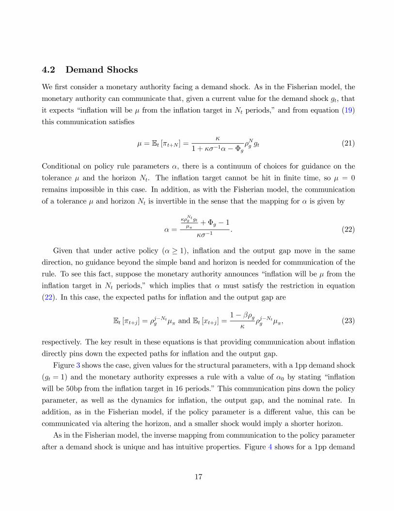
4.2 Demand Shocks

We first consider a monetary authority facing a demand shock. As in the Fisherian model, the

monetary authority can communicate that, given a current value for the demand shock gt, that

it expects “inflation will be µ from the inflation target in Nt periods,”and from equation (19)

this communication satisfies

µ = Et [πt+N ] =κ

1 + κσ−1α− Φg

ρNg gt (21)

Conditional on policy rule parameters α, there is a continuum of choices for guidance on the

tolerance µ and the horizon Nt. The inflation target cannot be hit in finite time, so µ = 0

remains impossible in this case. In addition, as with the Fisherian model, the communication

of a tolerance µ and horizon Nt is invertible in the sense that the mapping for α is given by

α =

κρNtg gtµπ

+ Φg − 1

κσ−1. (22)

Given that under active policy (α ≥ 1), inflation and the output gap move in the same

direction, no guidance beyond the simple band and horizon is needed for communication of the

rule. To see this fact, suppose the monetary authority announces “inflation will be µ from the

inflation target in Nt periods,”which implies that α must satisfy the restriction in equation

(22). In this case, the expected paths for inflation and the output gap are

Et [πt+j] = ρj−Ntg µπ and Et [xt+j] =1− βρg

κρj−Ntg µπ, (23)

respectively. The key result in these equations is that providing communication about inflation

directly pins down the expected paths for inflation and the output gap.

Figure 3 shows the case, given values for the structural parameters, with a 1pp demand shock

(gt = 1) and the monetary authority expresses a rule with a value of α0 by stating “inflation

will be 50bp from the inflation target in 16 periods.”This communication pins down the policy

parameter, as well as the dynamics for inflation, the output gap, and the nominal rate. In

addition, as in the Fisherian model, if the policy parameter is a different value, this can be

communicated via altering the horizon, and a smaller shock would imply a shorter horizon.

As in the Fisherian model, the inverse mapping from communication to the policy parameter

after a demand shock is unique and has intuitive properties. Figure 4 shows for a 1pp demand

17

Figure 3: Impulse Responses from a Demand Shock

0 2 4 6 8 10 12 14 16 18 200

1

2

3Inflation

0

1  (< 0)

2  (> 0)

0 wi th a smaller shock

0 2 4 6 8 10 12 14 16 18 200

0.5

1

1.5

2Output Gap

0 2 4 6 8 10 12 14 16 18 200

1

2

3

4Nominal Rate

Note: Shows impulse responses to a 1pp shock (0.66pp in the smaller shock case) to demandwhen β = 0.99, σ = 1, κ = 0.17, and ρg = 0.9. Values for the policy parameters areα0 = 1.40, α1 = 1.21, and α0 = 1.97.

shock, the implied policy parameter for given combinations of bands and horizons. Given a

horizon, smaller values for the band imply stronger reactions to inflation; meanwhile, given a

band size, longer horizons imply a weaker inflation response.

18

Figure 4: Effective Communication Pins Down the Policy Parameter after a Demand Shock

0 2 4 6 8 10 12 14 16 18 20N

1

1.5

2

2.5

3

3.5

4

4.5

5 = 1.50 = 0.50 = 0.25

Note: Shows the mapping from N and µ to α after a 1pp shock to the real interest rateβ = 0.99, σ = 1, κ = 0.17, and ρu = 0.95.

4.3 Supply Shocks

Now we consider a monetary authority that faces a supply shock. In this case, the monetary

authority could communicate that after a supply shock of ut, “inflation will be µ from the

inflation target in Nt periods,”and from equation (19) this communication satisfies

µ = Et [πt+N ] =1− ρu

1 + κσ−1α− Φu

ρNtu ut. (24)

Once again, there is a continuum of choices for guidance on the tolerance µ and the horizon

Nt conditional on policy rule parameter α, although µ = 0 is not feasible in finite time. As in

the case for a demand shock, the communication of a tolerance µ and horizon Nt is invertible

in the sense that the mapping for α is a function of the communication given the structural

parameters. In this case, the monetary authority could communicate that after a supply shock

of ut, “inflation will be µ from the inflation target in Nt periods,”and from equation (19) this

19

communication satisfies

α =

1−ρuµρNtu ut + Φu − 1

κσ−1. (25)

Similar to the demand shock only case, communication about inflation is suffi cient to pin

down the expected paths of inflation and the output gap if policy is active (α ≥ 1). The above

communication pins down α and the expected paths of inflation

Et [πt+j] = ρj−Ntu µ (26)

and the output gap

Et [xt+j] = − σ−1

1− ρu

(1−ρuµρNtu ut + Φu − 1

κσ−1− ρu

)ρj−Ntu µ. (27)

The key result from these equations is the independence from α, which highlights that providing

communication about inflation directly pins down the expected paths for inflation, the output

gap, and the interest rate without the need to specify the exact policy rule.

Figure 5 provides evidence that, given values for the structural parameters, after a 1pp

supply shock (ut = 1), the monetary authority can express a rule with a value of α0 by stating

“inflation will be 50bp from the inflation target in 16 periods.”This communication pins down

the policy parameter, as well as the dynamics for inflation, the output gap, and the nominal

rate. In addition, as in the Fisherian model, if the policy parameter is a different value, this can

be communicated via altering the horizon, and a smaller shock would imply a shorter horizon.

Figure 6 shows the inverse mapping from communication after a supply shock retains the

intuitive properties from the Fisherian model. A higher policy parameter can be communicated

with a relatively tighter band, or a shorter horizon.

5 Evaluating Monetary Policy Deviations

Having established that, in both a Fisherian and simple New Keynesian framework, communi-

cating a horizon for inflation to return to within a band from target substitutes for stating an

explicit policy rule, we now turn to how this environment can be used to evaluate monetary

policy deviations. The two models studied thus far are forward-looking, and hence there are no

dynamic implications for monetary policy shocks beyond the period in which they occur. We

20

Figure 5: Impulse Responses from a Supply Shock

0 2 4 6 8 10 12 14 16 18 200

0.5

1

1.5

2Inflation

0

1  (< 0)

2  (> 0)

0 wi th a smaller shock

0 2 4 6 8 10 12 14 16 18 20­6

­5

­4

­3

­2

Output Gap

0 2 4 6 8 10 12 14 16 18 200

0.5

1

1.5Nominal Rate

Note: Shows impulse responses to a 1pp shock (0.66pp in the smaller shock case) to supplywhen β = 0.99, σ = 1, κ = 0.17, and ρu = 0.95. Values for the policy parameters areα0 = 1.25, α1 = 1.19, and α0 = 1.57.

now therefore consider a model with a hybrid New Keynesian Phillips curve, given by

πt = (1− θ) πt−1 + θEt [πt+1] + κxt + ut.

The presence of lagged inflation on the aggregate supply equation means that previous inflation

deviations from target will affect current inflation, as price-setting has a backward-looking or

inertial component from indexation to lagged inflation.

21

Figure 6: Effective Communication Pins Down the Policy Parameter after a Supply Shock

0 2 4 6 8 10 12 14 16 18 20N

1

1.5

2

2.5 = 1.50 = 0.50 = 0.25

Note: Shows the mapping from N and µ to α after a 1pp shock to the real interest rateβ = 0.99, σ = 1, κ = 0.17, and ρu = 0.95.

In this case, the existence of an endogenous predetermined variable πt−1 implies there is no

longer a simple closed form solution for πt and xt, but instead there are solutions of the form

πt = Γπππt−1 + Γπggt + Γπuut + Γπηηt

xt = Γxππt−1 + Γxggt + Γxuut + Γxηηt

where Γj,k are functions of α. The expected paths of inflation and the output gap are given by

Et [πt+j] = Γj+1ππ πt−1 +

j∑k=0

Γj−kππ ρkgΓπggt +

j∑k=0

Γj−kππ ρkuΓπuut + ΓjππΓπηηt (28)

22

and

Et [xt+j] = ΓxπΓjπππt−1 +

(Γxπ

j−1∑k=0

Γj−1−kππ ρkgΓπg + Γxgρjg

)gt (29)

+

(Γxπ

j−1∑k=0

Γj−1−kππ ρkuΓπu + Γxuρju

)ut + ΓxπΓj−1ππ Γπηηt.

Assuming that inflation previously was at target, communication after a 1pp demand shock

that “inflation will be µ from the inflation target in Nt periods”implies

µ = Et [πt+Nt ] =Nt∑k=0

ΓNt−kππ ρkgΓπg (30)

and similarly for a 1pp supply shock

µ = Et [πt+Nt ] =Nt∑k=0

ΓNt−kππ ρkuΓπu. (31)

Now, to consider the impact of a monetary policy deviation, we focus on a demand shock.

Figure 7 shows that, given structural parameters and a 1pp demand shock in t = 0, a policy rule

can be communicated by stating “inflation will be 50bp from the inflation target in 12 periods.”

In periods after the initial shock, and absent any further shocks, the communication adjusts

accordingly as the horizon shortens. For example, by t = 10, the monetary authority would

state “inflation will be 50bp from the inflation target in 2 periods.”

However, now consider a case when in t = 10, 11, 12, the monetary authority introduces

an accommodative deviation (ηt < 0), which lowers the nominal interest rate and hence raises

inflation and the output gap over their expected paths. First, in each of those periods, the

expected return to µ no longer coincides with the original communication, so the expected

horizon now increases. In t = 12, the communication is still at Nt = 2 periods rather than

the expectation to be at target. Second, this change in communication, and a corresponding

assessment of ex ante statements and ex post outcomes, is a way to measure the deviations and

hence how closely the monetary authority is following the rule.

As noted in Section 2, central banks around the world state policy in terms of forecasts rather

than deviations from a rule. The communication strategy of tolerance bands and a horizon allows

deviations to be communicated by changing the forecast of when inflation will hit the tolerance

23

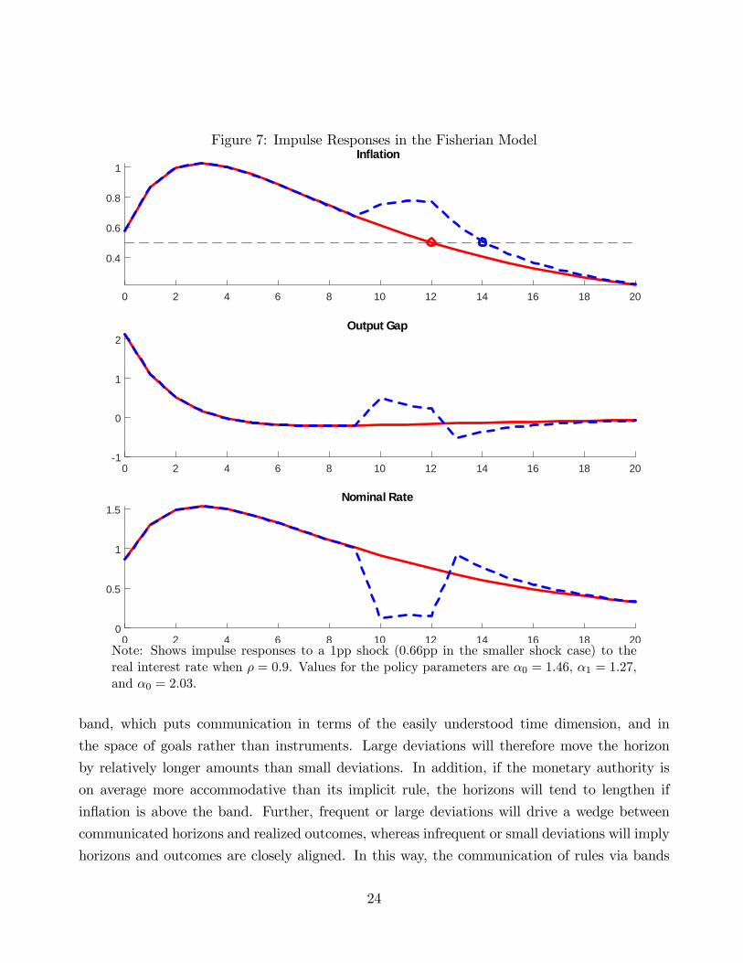
Figure 7: Impulse Responses in the Fisherian Model

0 2 4 6 8 10 12 14 16 18 20

0.4

0.6

0.8

1Inflation

0 2 4 6 8 10 12 14 16 18 20­1

0

1

2Output Gap

0 2 4 6 8 10 12 14 16 18 200

0.5

1

1.5Nominal Rate

Note: Shows impulse responses to a 1pp shock (0.66pp in the smaller shock case) to thereal interest rate when ρ = 0.9. Values for the policy parameters are α0 = 1.46, α1 = 1.27,and α0 = 2.03.

band, which puts communication in terms of the easily understood time dimension, and in

the space of goals rather than instruments. Large deviations will therefore move the horizon

by relatively longer amounts than small deviations. In addition, if the monetary authority is

on average more accommodative than its implicit rule, the horizons will tend to lengthen if

inflation is above the band. Further, frequent or large deviations will drive a wedge between

communicated horizons and realized outcomes, whereas infrequent or small deviations will imply

horizons and outcomes are closely aligned. In this way, the communication of rules via bands

24

and horizons creates a metric with which to evaluate central bank performance and adherence

to a rule. Lastly, we note that, in principle, the entire horizon of forecasts can be used to

evaluate performance. However, using the communication strategy here simplifies the metric

significantly, which is a key consideration for transparency.

6 Price Level Targeting

In this section, we extend the communication strategy to an additional type of policy rule,

that of price level targeting, and show the fundamental concept of bands and a horizon remains

unchanged. Price level targeting is an interesting extension because it has a make-up component

and has received attention in light of lower inflation and zero lower bound risk. More crucially, by

changing from inflation to price level targeting, the target for monetary policy changes, leading

to a necessary change in language.

To illustrate this environment, we return to the New Keynesian model in Section 4, but with

an interest rate rule given by

it = αpt + ηt (32)

where pt denotes deviations from the price level, which follows

pt = pt−1 + πt. (33)

As in examples considered, a monetary authority simply giving the stance of policy it does

not pin down a unique value of the policy parameter α and the deviation from the rule ηt, and

communicating α directly is not typically followed by central banks around the world. Again,

the existence of an endogenous predetermined variable pt−1 implies there is no longer a simple

closed-form solution for πt and xt, but instead there are solutions of the form

πt = Γπppt−1 + Γπggt + Γπuut + Γπηηt

xt = Γxppt−1 + Γxggt + Γxuut + Γxηηt

pt = Γpppt−1 + Γpggt + Γpuut + Γpηηt

25

where Γj,k are functions of α. The expected path for the price level is

Et [pt+j] = Γj+1pp pt−1 +

j∑k=0

Γj−kpp ρkgΓpggt +

j∑k=0

Γj−kpp ρkuΓpuut + ΓjppΓpηηt, (34)

which implies

Et [πt+j] = ΓπpΓjpppt−1 +

(Γπp

j−1∑k=0

Γj−1−kpp ρkgΓpg + Γπgρjj

)gt (35)

+

(Γπp

j−1∑k=0

Γj−1−kpp ρkuΓpu + Γπuρju

)ut + ΓπpΓ

j−1pp Γpηηt

and

Et [xt+j] = ΓxpΓjpppt−1 +

(Γxp

j−1∑k=0

Γj−1−kpp ρkgΓpg + Γxgρjj

)gt (36)

+

(Γxp

j−1∑k=0

Γj−1−kpp ρkuΓpu + Γxuρju

)ut + ΓxpΓ

j−1pp Γpηηt

Assuming that the price level was previously was at target, communication after a 1pp

demand shock that “inflation will be µ from the inflation target in Nt periods”implies

µ = Et [pt+N ] =

j∑k=0

Γj−kpp ρkgΓpg (37)

and similarly for a 1pp supply shock

Et [pt+N ] =

j∑k=0

Γj−kpp ρkuΓpu. (38)

In this case of price level targeting, then, policy can be communicated with “the price level

will be µ from the inflation target in Nt periods.”Figure 8 shows the case when, given values for

the structural parameters, after a 1pp demand shock (gt = 1) the monetary authority expresses a

rule with a value of α0 by stating “the price level will be 25bp from the inflation target in 8 peri-

ods.”This communication pins down the policy parameter, as well as the dynamics for inflation,

the output gap, and the nominal rate. A more dovish policy α1 can be communicated by stating

26

Figure 8: Impulse Responses with a Price Level Target Rule

0 2 4 6 8 10 12 14 160

0.2

0.4

0.6Price Level

0

1  (< 0)

0 2 4 6 8 10 12 14 160

0.2

0.4

Inflation

0 2 4 6 8 10 12 14 160

0.5

1

Output Gap

0 2 4 6 8 10 12 14 160.2

0.4

0.6

Nominal Rate

Note: Shows impulse responses to a 1pp shock to demand when β = 0.99, σ = 1, κ = 0.17,and ρg = 0.9. Values for the policy parameters are α0 = 1.63 and α1 = 1.04.

“the price level will be 25bp from the inflation target in 12 periods.”These communications pin

down inflation, the output gap, and the nominal rate. In addition, by changing communication

to the price level, the central bank preserves the principles for measuring deviations as discussed

in the previous section.

27

7 Conclusion

Motivated by the wide-ranging communication strategies of the central banks around the world

that use some form of inflation targeting, we develop a link between rules-based monetary policy

and effective communication. Our framework relies on three key features: the specification of

a point inflation target, tolerance bands around the point, and economic projections. In simple

Fisherian and New Keynesian models, we show that effective communication about the band and

a horizon for achieving that band given shocks can implicitly pin down a rule without having

to explicitly express one. In addition, the results suggest that communicating rules in this

way generates a metric with which to evaluate deviations from the implicit rule by comparing

communication with realized outcomes. The form of the communication can easily be extended

to alternative rules such as price-level targeting. Central banks that use this communication

can then reap the benefits of rules-based policy without necessarily having to codify their rule.

References

Andersson, Fredrik and Lars Jonung. 2017. “Inflation Targets and the Benefits of an Explicit

Tolerance Band.”Vox EU. May 8.

Banco Central Do Brasil. 2016. “Inflation Targeting Regime in Brazil.”Frequently Asked Ques-

tions Series.

Battini, Nicoletta and Edward Nelson. 2001. “Optimal Horizons for Inflation Targeting.”Journal

of Economic Dynamics and Control .

Bernanke, Ben and Frederic Mishkin. 1997. “Inflation Targeting: A New Framework for Mone-

tary Policy?” Journal of Economic Perspectives 11(2):97—116.

Cecchetti, Stephen G. and Kermit L. Schoenholtz. 2019. “Improving U.S. Monetary Policy

Communications.”Mimeo.

Central Bank News. 2021. “Inflation Targets Table for 2021.”http://www.centralbanknews.

info/p/inflation-targets.html. Accessed February 17, 2021.

Choi, Jason and Andrew Foerster. 2019. Optimal Monetary Policy Regime Switches. Working

Paper 2019-3 Federal Reserve Bank of San Francisco.

28

Cochrane, John and John Taylor, eds. 2016. Central Bank Governance and Oversight Reform.

The Hoover Institution.

Coibion, Olivier, Yuriy Gorodnichenko and Michael Weber. 2019. Monetary Policy Communi-

cations and their Effects on Household Inflation Expectations. Working Papers 25482 NBER.

D’Acunto, Francesco, Daniel Hoang, Maritta Paloviita and Michael Weber. 2019. Human fric-

tions in the transmission of economic policy. Working Paper Series in Economics 128 Karlsruhe

Institute of Technology (KIT), Department of Economics and Business Engineering.

Erceg, Christopher. 2002. “The Choice of an Inflation Target Range in a Small Open Economy.”

American Economic Review 92(2):85—89.

Fuhrer, Jeffrey C., Giovanni P. Olivei, Eric S. Rosengren and Geoffrey M. B. Tootell. 2018.

Should the Fed Regularly Evaluate its Monetary Policy Framework? Working Papers 18-8

Federal Reserve Bank of Boston.

Heikensten, Lars. 1999. “The Riksbank’s Inflation Target - Clarification and Evaluation.”

Sveriges Riksbank Quarterly Review 1999(1):5—17.

Ikeda, Daisuke and Takushi Kurozumi. 2014. Post-Crisis Slow Recovery and Monetary Policy.

IMES Discussion Paper Series 14-E-16 Institute for Monetary and Economic Studies, Bank

of Japan.

McDermott, John and Rebecca Williams. 2018. “Inflation Targeting in New Zealand: An

Experience in Evolution.”Speech delivered to the Reserve Bank of Australia conference on

central bank frameworks. April 12.

Mishkin, Frederic S. and Niklas J. Westelius. 2008. “Inflation Band Targeting and Optimal

Inflation Contracts.”Journal of Money, Credit and Banking 40(4):557—582.

Orphanides, Athanasios. 2019. “Monetary Policy Strategy and its Communication.”Mimeo.

Orphanides, Athanasios and Volker Weiland. 2000. “Inflation Zone Targeting.”European Eco-

nomic Review 44(7):1351—1387.

Riksbank. 2010. “The Riksbank Removes the Tolerance Interval from its Specified Monetary

Policy Target.”Monetary Policy Department. Decision - 31 May 2010.

29

Riksbank. 2016. “The Riksbank’s Inflation Target - Target Variable and Interval.”Riksbank

Studies.

Schmitt-Grohe, Stephanie and Martin Uribe. 2007. “Optimal Simple and Implementable Mon-

etary and Fiscal Rules.”Journal of Monetary Economics 54(6):1702—1725.

Smets, Frank. 2000. “What Horizon for Price Stability.”European Central Bank Working Paper

No. 24.

Svensson, Lars E. O. 1999. “Inflation Targeting as a Monetary Policy Rule.”Journal of Monetary

Economics 43(3):607—654.

Svensson, Lars E.O. 2002. “Inflation Targeting: Should it be Modeled as an Instrument Rule

or a Targeting Rule?”European Economic Review 46(4-5):771—780.

Svensson, Lars E.O. and Michael Woodford. 2005. Limits to Inflation Targeting. In Implement-

ing Optimal Policy through Inflation-Forecast Targeting, ed. Ben S. Bernanke and Michael

Woodford. Chicago: The University of Chicago Press pp. 19—91.

Walsh, Carl. 1995. “Optimal Contracts for Central Bankers.” American Economic Review

85:150—167.

Walsh, Carl. 2015. “Goals and Rules in Central Bank Design.”International Journal of Central

Banking 11(S1):295—352.

Warsh, Kevin. 2017. “America Needs a Steady, Strategic Fed.”Wall Street Journal. January

30.

Woodford, Michael. 2005. Central-Bank Communication and Policy Effectiveness. In The

Greenspan Era: Lessons for the Future. Jackson Hole, Wyoming: Federal Reserve Bank

of Kansas City pp. 399—474.

30