Common Information Model Power System Dynamics Standard ...
115
Common Information Model for Power System Dynamics Standard Dynamic Model Reference Document DRAFT November 30, 2008
Transcript of Common Information Model Power System Dynamics Standard ...
Common Information Model for
Power System Dynamics
Standard Dynamic Model Reference Document
DRAFT November 30, 2008
Page 2
Introduction ............................................................................................................................................................................. 4
Standard Interconnections ................................................................................................................................................... 5
Synchronous Generator Unit............................................................................................................................................................................. 5 Asynchronous (Induction) Generator Unit ................................................................................................................................................... 7 Large Synchronous Motor Unit ........................................................................................................................................................................ 8 Large Asynchronous (Induction) Motor Unit ............................................................................................................................................... 9 Aggregate Load.....................................................................................................................................................................................................10
Synchronous Generator Models......................................................................................................................................... 11
genSync - Synchronous Generator Model ..............................................................................................................................................13 genSync - RoundRotor Type....................................................................................................................................................................17 genSync - Salient Pole Type......................................................................................................................................................................19 genSync - Transient Type .........................................................................................................................................................................20 genSync - TypeF.............................................................................................................................................................................................20 genSync - TypeJ .............................................................................................................................................................................................21 genSync - CrossCompound Type...........................................................................................................................................................22
genEquiv - Equivalent (Classical ) Generator Model..............................................................................................................................24
Asynchronous Generator Models ...................................................................................................................................... 26
genAsync - Asynchronous Generator Model...........................................................................................................................................28
Large Synchronous Motor Models ..................................................................................................................................... 31
motorSync - Synchronous Motor Model....................................................................................................................................................33 motorSync - RoundRotor Type...............................................................................................................................................................38 motorSync - Salient Pole Type.................................................................................................................................................................40
Large Asynchronous Motor Models................................................................................................................................... 41
motorAsync - Asynchronous Motor Model...............................................................................................................................................42
Voltage Compensation Models .......................................................................................................................................... 45
vcompIEEE - IEEE Voltage Compensation Model....................................................................................................................................47 vcompCross – Cross-Compound Voltage Compensation Model.....................................................................................................48
Excitation System Models.................................................................................................................................................... 49
excAC1A - IEEE AC1A Model ............................................................................................................................................................................51 excAC2A - IEEE AC2A Model ............................................................................................................................................................................53 excAC3A - IEEE AC3A Model ............................................................................................................................................................................55 excAC4A - IEEE AC4A Model ............................................................................................................................................................................57 excAC5A - IEEE AC5A Model ............................................................................................................................................................................59 excAC6A - IEEE AC6A Model ............................................................................................................................................................................61 excAC7B - IEEE AC7B Model ............................................................................................................................................................................63
Page 3
excAC8B - IEEE AC8B Model ............................................................................................................................................................................65 excDC1A - IEEE DC1A Model............................................................................................................................................................................67 excDC2A - IEEE DC2A Model............................................................................................................................................................................69 excDC3A - IEEE DC3A Model............................................................................................................................................................................71 excDC4B - IEEE DC4B Model............................................................................................................................................................................73 excST1A - IEEE ST1A Model..............................................................................................................................................................................75 excST2A - IEEE ST2A Model..............................................................................................................................................................................77 excST3A - IEEE ST3A Model..............................................................................................................................................................................79 excST4B - IEEE ST4B Model..............................................................................................................................................................................81 excST5B - IEEE ST5B Model..............................................................................................................................................................................83 excST6B - IEEE ST6B Model..............................................................................................................................................................................85 excST7B - IEEE ST7B Model..............................................................................................................................................................................87 Other Excitation System Models To Be Added.........................................................................................................................................89
Power System Stabilizer (PSS) Models ............................................................................................................................... 90
pssIEEE2B - IEEE PSS2B Power System Stabilizer Model .................................................................................................................92 Other PSS Models To Be Added......................................................................................................................................................................94
Turbine-Governor Models ................................................................................................................................................... 95
govHydro1 – Hydro Turbine-Governor Model .........................................................................................................................................97 govSteam1 – IEEE Steam Turbine-Governor Model.............................................................................................................................99 govPID1 – General PID Governor and Prime Mover Model ...........................................................................................................102 Other Turbine-Governor Models That May Be Added .......................................................................................................................106
Aggregate Load Models..................................................................................................................................................... 107
loadStatic - Static Load Model...................................................................................................................................................................109 loadMotor - Aggregate Induction Motor Load ...................................................................................................................................111
Mechanical Load Models ................................................................................................................................................... 114
mechload1 - Mechanical Load Model 1 ................................................................................................................................................115
Page 4
Introduction The CIM standard dynamic models include most models for power system equipment that are commonly used for analysis of power system dynamic simulations in the transient and oscillatory stability time scale as defined by IEEE / CIGRE Standard Terms and Definitions for Power System Stability Analysis [ref]. Each of the models is described in this document, grouped by type of model.
Page 5
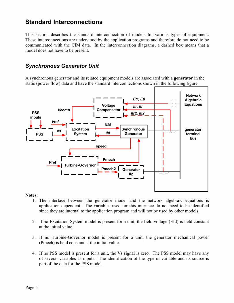
Standard Interconnections This section describes the standard interconnection of models for various types of equipment. These interconnections are understood by the application programs and therefore do not need to be communicated with the CIM data. In the interconnection diagrams, a dashed box means that a model does not have to be present.
Synchronous Generator Unit A synchronous generator and its related equipment models are associated with a generator in the static (power flow) data and have the standard interconnections shown in the following figure.
IfdExcitation
System
Efd
Turbine-Governor
Vcomp
speed
Pmech
PSSVs
Voltage Compensator
Etr, Eti
Itr, Iti
SynchronousGenerator
generatorterminal
bus
Network Algebraic Equations
Pref
PSS inputs
Itr2, Iti2
Generator#2
Vref
Pmech2
Notes:
1. The interface between the generator model and the network algebraic equations is application dependent. The variables used for this interface do not need to be identified since they are internal to the application program and will not be used by other models.
2. If no Excitation System model is present for a unit, the field voltage (Efd) is held constant
at the initial value.
3. If no Turbine-Governor model is present for a unit, the generator mechanical power (Pmech) is held constant at the initial value.
4. If no PSS model is present for a unit, the Vs signal is zero. The PSS model may have any of several variables as inputs. The identification of the type of variable and its source is part of the data for the PSS model.
Page 6
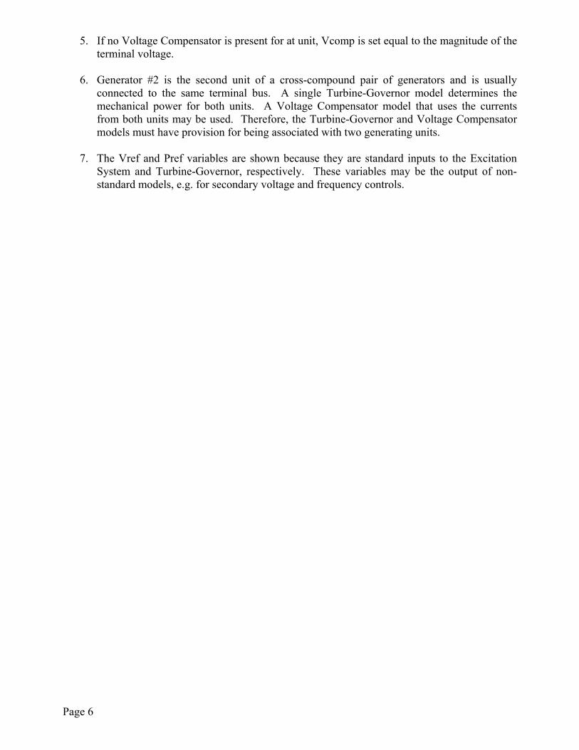
5. If no Voltage Compensator is present for at unit, Vcomp is set equal to the magnitude of the terminal voltage.
6. Generator #2 is the second unit of a cross-compound pair of generators and is usually connected to the same terminal bus. A single Turbine-Governor model determines the mechanical power for both units. A Voltage Compensator model that uses the currents from both units may be used. Therefore, the Turbine-Governor and Voltage Compensator models must have provision for being associated with two generating units.
7. The Vref and Pref variables are shown because they are standard inputs to the Excitation System and Turbine-Governor, respectively. These variables may be the output of non-standard models, e.g. for secondary voltage and frequency controls.
Page 7
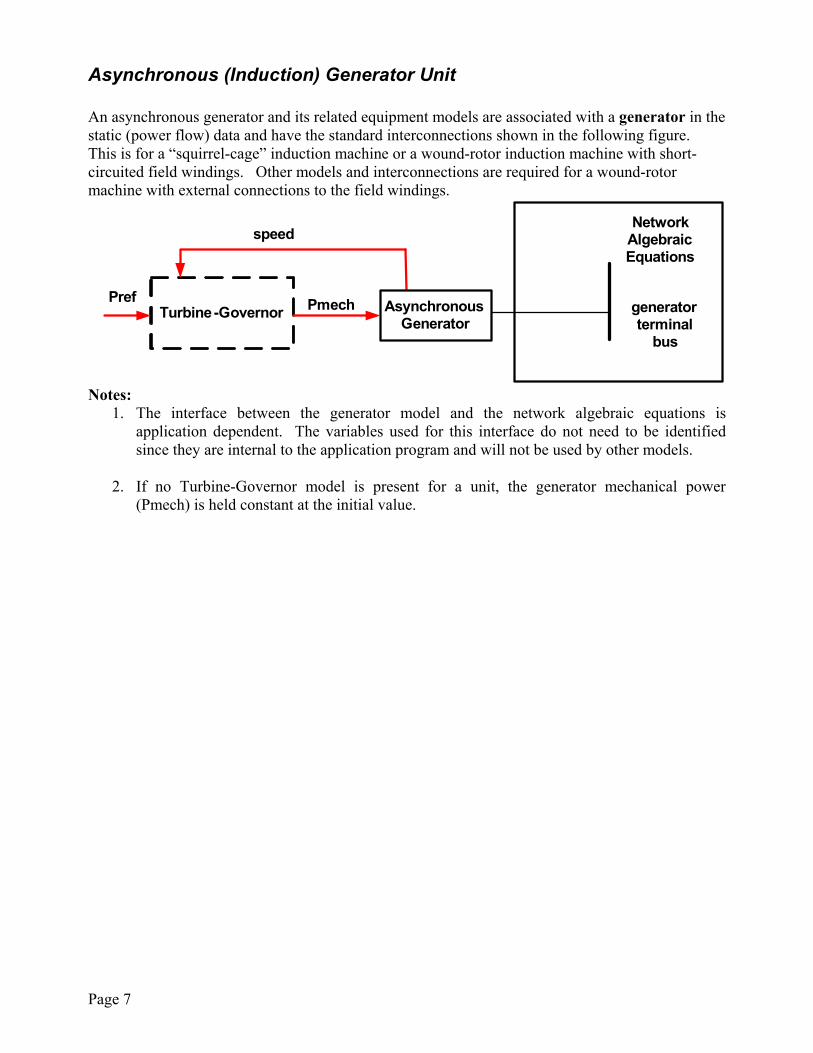
Asynchronous (Induction) Generator Unit An asynchronous generator and its related equipment models are associated with a generator in the static (power flow) data and have the standard interconnections shown in the following figure. This is for a “squirrel-cage” induction machine or a wound-rotor induction machine with short-circuited field windings. Other models and interconnections are required for a wound-rotor machine with external connections to the field windings.
Turbine-Governor
speed
Pmech AsynchronousGenerator
generatorterminal
bus
Network Algebraic Equations
Pref
Notes:
1. The interface between the generator model and the network algebraic equations is application dependent. The variables used for this interface do not need to be identified since they are internal to the application program and will not be used by other models.
2. If no Turbine-Governor model is present for a unit, the generator mechanical power
(Pmech) is held constant at the initial value.
Page 8
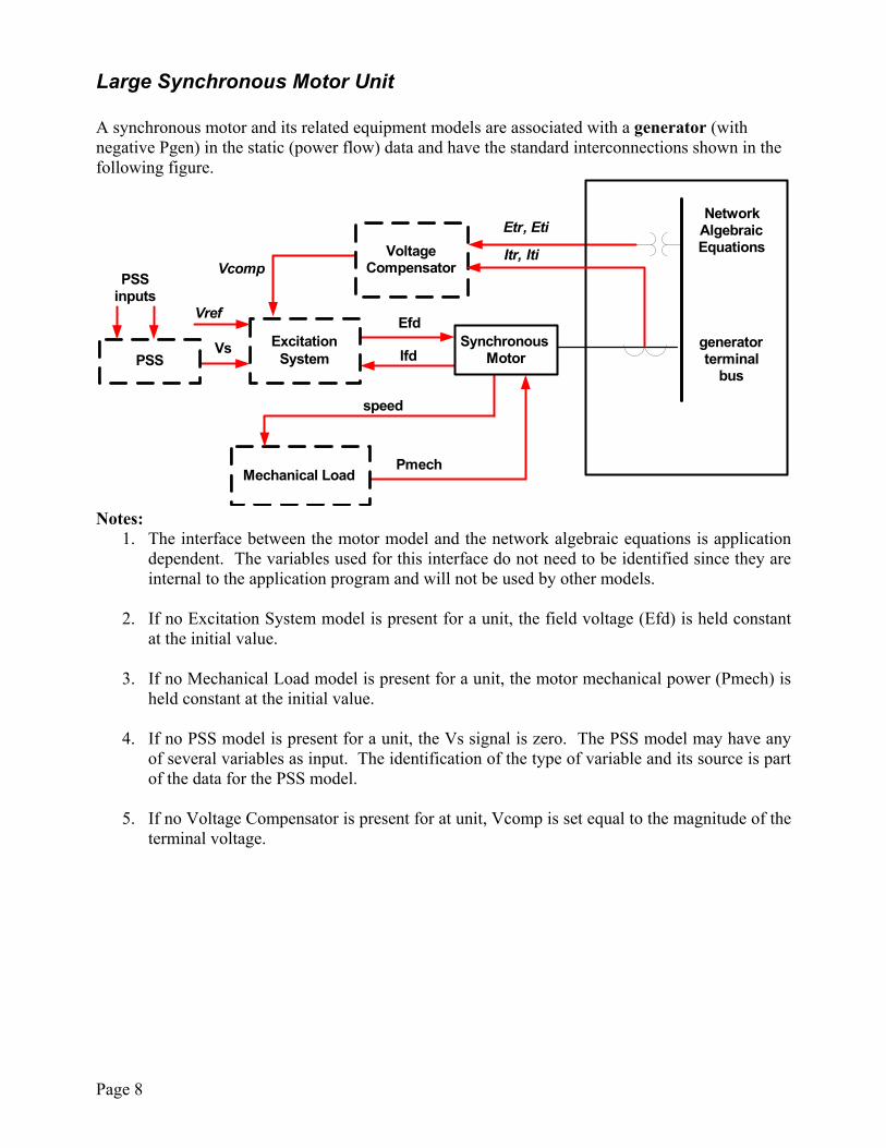
Large Synchronous Motor Unit A synchronous motor and its related equipment models are associated with a generator (with negative Pgen) in the static (power flow) data and have the standard interconnections shown in the following figure.
IfdExcitation
System
Efd
Mechanical Load
Vcomp
speed
Pmech
PSSVs
Voltage Compensator
Etr, Eti
Itr, Iti
SynchronousMotor
generatorterminal
bus
Network Algebraic Equations
PSS inputs
Vref
Notes:
1. The interface between the motor model and the network algebraic equations is application dependent. The variables used for this interface do not need to be identified since they are internal to the application program and will not be used by other models.
2. If no Excitation System model is present for a unit, the field voltage (Efd) is held constant
at the initial value.
3. If no Mechanical Load model is present for a unit, the motor mechanical power (Pmech) is held constant at the initial value.
4. If no PSS model is present for a unit, the Vs signal is zero. The PSS model may have any of several variables as input. The identification of the type of variable and its source is part of the data for the PSS model.
5. If no Voltage Compensator is present for at unit, Vcomp is set equal to the magnitude of the terminal voltage.
Page 9
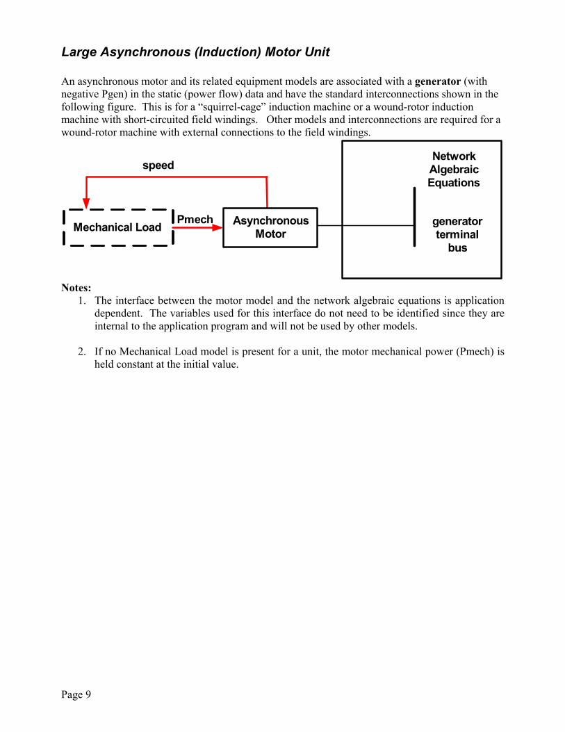
Large Asynchronous (Induction) Motor Unit An asynchronous motor and its related equipment models are associated with a generator (with negative Pgen) in the static (power flow) data and have the standard interconnections shown in the following figure. This is for a “squirrel-cage” induction machine or a wound-rotor induction machine with short-circuited field windings. Other models and interconnections are required for a wound-rotor machine with external connections to the field windings.
Mechanical Load
speed
Pmech Asynchronous Motor
generatorterminal
bus
Network Algebraic Equations
Notes:
1. The interface between the motor model and the network algebraic equations is application dependent. The variables used for this interface do not need to be identified since they are internal to the application program and will not be used by other models.
2. If no Mechanical Load model is present for a unit, the motor mechanical power (Pmech) is
held constant at the initial value.
Page 10
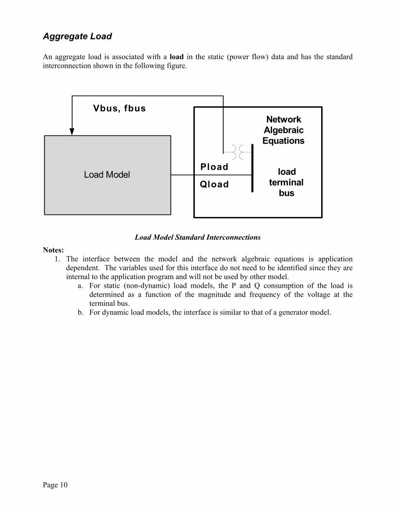
Aggregate Load An aggregate load is associated with a load in the static (power flow) data and has the standard interconnection shown in the following figure.
Pload
Vbus, fbus
Load ModelQload
loadterminal
bus
Network Algebraic Equations
Load Model Standard Interconnections
Notes: 1. The interface between the model and the network algebraic equations is application
dependent. The variables used for this interface do not need to be identified since they are internal to the application program and will not be used by other model.
a. For static (non-dynamic) load models, the P and Q consumption of the load is determined as a function of the magnitude and frequency of the voltage at the terminal bus.
b. For dynamic load models, the interface is similar to that of a generator model.
Page 11
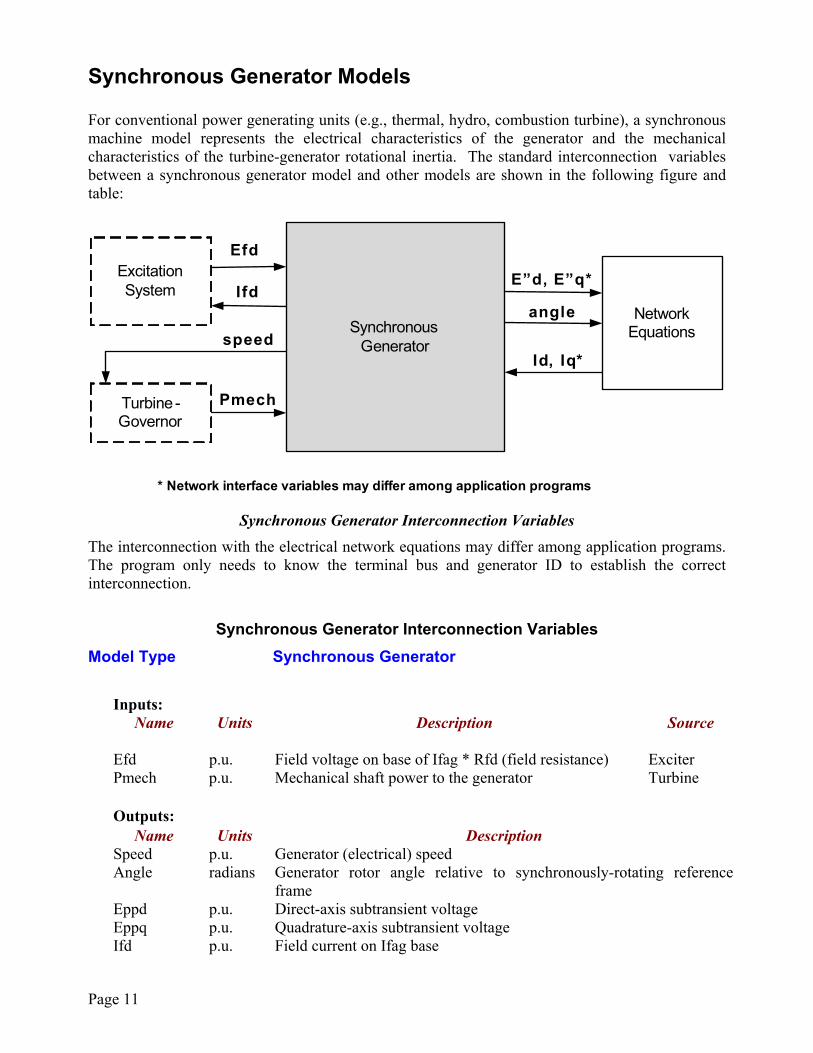
Synchronous Generator Models For conventional power generating units (e.g., thermal, hydro, combustion turbine), a synchronous machine model represents the electrical characteristics of the generator and the mechanical characteristics of the turbine-generator rotational inertia. The standard interconnection variables between a synchronous generator model and other models are shown in the following figure and table:
Efd
SynchronousGenerator
Pmech
Network Equations
Turbine -Governor
Excitation System I fd
speedId, Iq*
E”d, E”q*
* Network interface variables may differ among application programs
angle
Synchronous Generator Interconnection Variables
The interconnection with the electrical network equations may differ among application programs. The program only needs to know the terminal bus and generator ID to establish the correct interconnection.
Synchronous Generator Interconnection Variables
Model Type Synchronous Generator
Inputs: Name
Units Description Source
Efd p.u. Field voltage on base of Ifag * Rfd (field resistance) Exciter Pmech p.u. Mechanical shaft power to the generator Turbine Outputs: Name Units Description Speed p.u. Generator (electrical) speed Angle radians Generator rotor angle relative to synchronously-rotating reference
frame Eppd p.u. Direct-axis subtransient voltage Eppq p.u. Quadrature-axis subtransient voltage Ifd p.u. Field current on Ifag base
Page 12
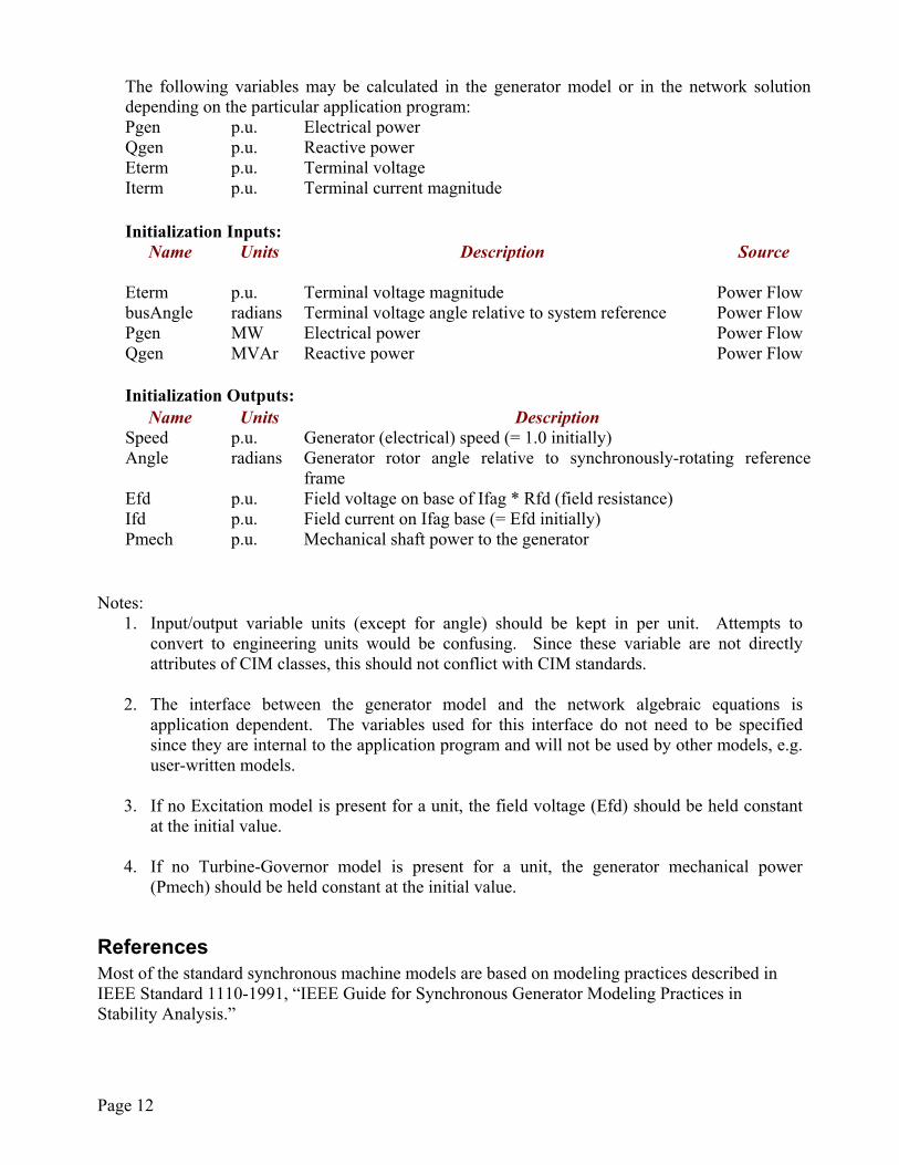
The following variables may be calculated in the generator model or in the network solution
depending on the particular application program: Pgen p.u. Electrical power Qgen p.u. Reactive power Eterm p.u. Terminal voltage Iterm p.u. Terminal current magnitude Initialization Inputs: Name
Units Description Source
Eterm p.u. Terminal voltage magnitude Power Flow busAngle radians Terminal voltage angle relative to system reference Power Flow Pgen MW Electrical power Power Flow Qgen MVAr Reactive power Power Flow Initialization Outputs: Name Units Description Speed p.u. Generator (electrical) speed (= 1.0 initially) Angle radians Generator rotor angle relative to synchronously-rotating reference
frame Efd p.u. Field voltage on base of Ifag * Rfd (field resistance) Ifd p.u. Field current on Ifag base (= Efd initially) Pmech p.u. Mechanical shaft power to the generator Notes:
1. Input/output variable units (except for angle) should be kept in per unit. Attempts to convert to engineering units would be confusing. Since these variable are not directly attributes of CIM classes, this should not conflict with CIM standards.
2. The interface between the generator model and the network algebraic equations is
application dependent. The variables used for this interface do not need to be specified since they are internal to the application program and will not be used by other models, e.g. user-written models.
3. If no Excitation model is present for a unit, the field voltage (Efd) should be held constant
at the initial value.
4. If no Turbine-Governor model is present for a unit, the generator mechanical power (Pmech) should be held constant at the initial value.
References Most of the standard synchronous machine models are based on modeling practices described in IEEE Standard 1110-1991, “IEEE Guide for Synchronous Generator Modeling Practices in Stability Analysis.”
Page 13
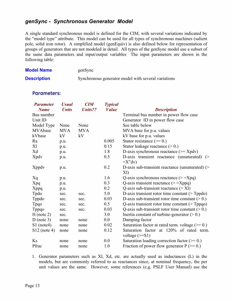
genSync - Synchronous Generator Model A single standard synchronous model is defined for the CIM, with several variations indicated by the “model type” attribute. This model can be used for all types of synchronous machines (salient pole, solid iron rotor). A simplified model (genEquiv) is also defined below for representation of groups of generators that are not modeled in detail. All types of the genSync model use a subset of the same data parameters and input/output variables The input parameters are shown in the following table: Model Name genSync
Description Synchronous generator model with several variations
Parameters:
Parameter Usual CIM Typical Name Units Units?? Value Description Bus number Terminal bus number in power flow case Unit ID Generator ID in power flow case Model Type None None See table below MVAbase MVA MVA MVA base for p.u. values kVbase kV kV kV base for p.u. values Ra p.u. 0.005 Stator resistance (>= 0.) Xl p.u. 0.15 Stator leakage reactance (> 0.) Xd p.u. 1.8 D-axis synchronous reactance (>= Xpdv) Xpdv p.u. 0.5 D-axis transient reactance (unsaturated) (>
=X”dv) Xppdv p.u. 0.2 D-axis sub-transient reactance (unsaturated) (>
Xl) Xq p.u. 1.6 Q-axis synchronous reactance (> =Xpq) Xpq p.u. 0.3 Q-axis transient reactance (> =Xppq) Xppq p.u. 0.2 Q-axis sub-transient reactance (> Xl) Tpdo sec. sec. 5.0 D-axis transient rotor time constant (> Tppdo) Tppdo sec. sec. 0.03 D-axis sub-transient rotor time constant (> 0.) Tpqo sec. sec. 0.5 Q-axis transient rotor time constant (> Tppqo) Tppqo sec. sec. 0.03 Q-axis sub-transient rotor time constant (> 0.) H (note 2) sec. 3.0 Inertia constant of turbine-generator (> 0.) D (note 3) none none 0.0 Damping factor S1 (note4) none none 0.02 Saturation factor at rated term. voltage (>= 0.) S12 (note 4) none none 0.12 Saturation factor at 120% of rated term.
voltage (>=S1) Ks none none 0.0 Saturation loading correction factor (>= 0.) Pfrac none none 1.0 Fraction of power flow generator P (>= 0.)
1. Generator parameters such as Xl, Xd, etc. are actually used as inductances (L) in the models, but are commonly referred to as reactances since, at nominal frequency, the per unit values are the same. However, some references (e.g. PSLF User Manual) use the
Page 14
symbol L instead of X. Also, the “p” in the parameter names is a substitution for a “prime” in the usual notation, e.g. Xppd refers to X”d.
2. H is the stored energy in the rotating mass of the generator plus all other elements (turbine, exciter) on the same shaft and has units of MW-sec. Conventional units are per unit on the generator MVA base, usually expressed as MW-sec./MVA or just sec. (since MW and MVA are equivalent units).
3. D has units of power/speed but is regarded as a dimensionless factor resulting from
linearization of an exponential relationship between speed and power: ( )DoPP ω= . This value is often zero when the source of damping torques (generator damper windings, load damping effects, etc.) are modeling in detail. [ref]
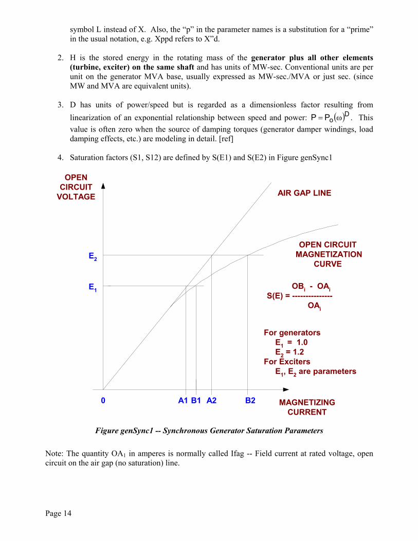
4. Saturation factors (S1, S12) are defined by S(E1) and S(E2) in Figure genSync1
E1
OPENCIRCUIT
VOLTAGE
OPEN CIRCUIT MAGNETIZATION
CURVE
MAGNETIZINGCURRENT
For generators E1 = 1.0 E2 = 1.2For Exciters E1, E2 are parameters
E2
A1 B1 A2 B2
AIR GAP LINE
0
OBi - OAi S(E) = --------------- OAi
Figure genSync1 -- Synchronous Generator Saturation Parameters
Note: The quantity OA1 in amperes is normally called Ifag -- Field current at rated voltage, open circuit on the air gap (no saturation) line.
Page 15
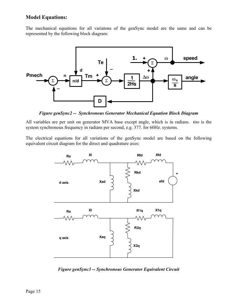
Model Equations: The mechanical equations for all variatons of the genSync model are the same and can be represented by the following block diagram:
12Hs
∆ω
D
Tespeed
anglePmech
1. +
ωos
+
Σ+
_
_
ω
n/dn Tm
d
Σ
Σ
Figure genSync2 -- Synchronous Generator Mechanical Equation Block Diagram
All variables are per unit on generator MVA base except angle, which is in radians. ωo is the system synchronous frequency in radians per second, e.g. 377. for 60Hz. systems. The electrical equations for all variations of the genSync model are based on the following equivalent circuit diagram for the direct and quadrature axes:
+
efd
Xl Xfd
Xkd
Xad
Rkd
Ra Rfd
d axis
Xl X1q
X2q
Xaq
R2q
Ra R1q
q axis
Figure genSync3 -- Synchronous Generator Equivalent Circuit
Page 16
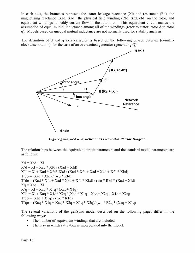
In each axis, the branches represent the stator leakage reactance (Xl) and resistance (Ra), the magnetizing reactance (Xad, Xaq), the physical field winding (Rfd, Xfd, efd) on the rotor, and equivalent windings for eddy current flow in the rotor iron. This equivalent circuit makes the assumption of equal mutual inductance among all of the windings (rotor to stator, rotor d to rotor q). Models based on unequal mutual inductance are not normally used for stability analysis. The definition of d and q axis variables is based on the following phasor diagram (counter-clockwise rotation), for the case of an overexcited generator (generating Q):
q axis
Et
It
It (Ra + jX”)
E”
j It ( Xq-X”)
d axis
Network Reference
rotor angle
bus angle
Figure genSync4 -- Synchronous Generator Phasor Diagram
The relationships between the equivalent circuit parameters and the standard model parameters are as follows: Xd = Xad + Xl X’d = Xl + Xad * Xfd / (Xad + Xfd) X”d = Xl + Xad * Xfd* Xkd / (Xad * Xfd + Xad * Xkd + Xfd * Xkd) T’do = (Xad + Xfd) / (wo * Rfd) T”do = (Xad * Xfd + Xad * Xkd + Xfd * Xkd) / (wo * Rkd * (Xad + Xfd) Xq = Xaq + Xl X’q = Xl + Xaq * X1q / (Xaq+ X1q) X”q = Xl + Xaq * X1q* X2q / (Xaq * X1q + Xaq * X2q + X1q * X2q) T’qo = (Xaq + X1q) / (wo * R1q) T”qo = (Xaq * X1q + Xaq * X2q + X1q * X2q)/ (wo * R2q * (Xaq + X1q) The several variations of the genSync model described on the following pages differ in the following ways:
• The number of equivalent windings that are included • The way in which saturation is incorporated into the model.
Page 17
• Whether or not “subtransient saliency” (Xppq ≠ Xppdv) is represented. • Whether or not multiple units (e.g. cross-compound set) are represented individually in the
static (power flow) data. Variations of the genSync model are identified by the “model type” attribute as shown in the table below, together with the corresponding model names in each application program. Each model type is described in detail on the following pages. CIM PSLF PSS/E DigSilent Eurostag Model Type Model Model Model Model RoundRotor genrou GENROU ElmSym SalientPole gensal GENSAL ElmSym Transient (genrou) GENTRA ElmSym TypeF gentpf TypeJ gentpj CrossCompound gencc GENROU? Note: It is not necessary for each program to have separate models for each of the model types. The same model can often be used for several types by alternative logic within the model. Also, differences in saturation representation may not result in significant model performance differences so model substitutions are often acceptable.
genSync - RoundRotor Type The complete equivalent circuit is used with two rotor windings in each axis. Notes:
• Xppq is assumed to be equal to Xppd (no subtransient saliency) • Saturation is modeled in both the d and q axes as shown in the block diagram • The following input parameters are not used: Xppq, Ks, Pfrac
Block Diagram:

Page 18
Se
XlXdXlXq
−−
ψ" = sqrt(ψ"d2+ψ"d
2)ψ"d
ψ"q
do''sT1
2**)Xld'X(d''Xd'X
−− X'd-Xl d-AXIS
Efddo'sT
1Xld'X
d''Xd'X−
−
Xld'XXld''X
−−
Xd-X'dIfd
ψfdψkd
qo''sT1
2**)Xlq'X(q''Xq'X
−−
X'q-Xl q-AXIS
iq
qo'sT1
Xlq'Xq'Xq'X
−−
Xlq'XXlq''X
−−
Xq-X'q
ψ1qψ2q
ψ"q
iq
id
X''d
Ra
Eq
id
Σ
X''q
Ra
Ed
ψ"dΠ
ω
Π
ω
ΣΣ
ΣΣ
Σ
Σ
Σ Σ
ΣΣ Σ
Figure genSync5 -- genSync – RoundRotor Type Model Block Diagram
Page 19
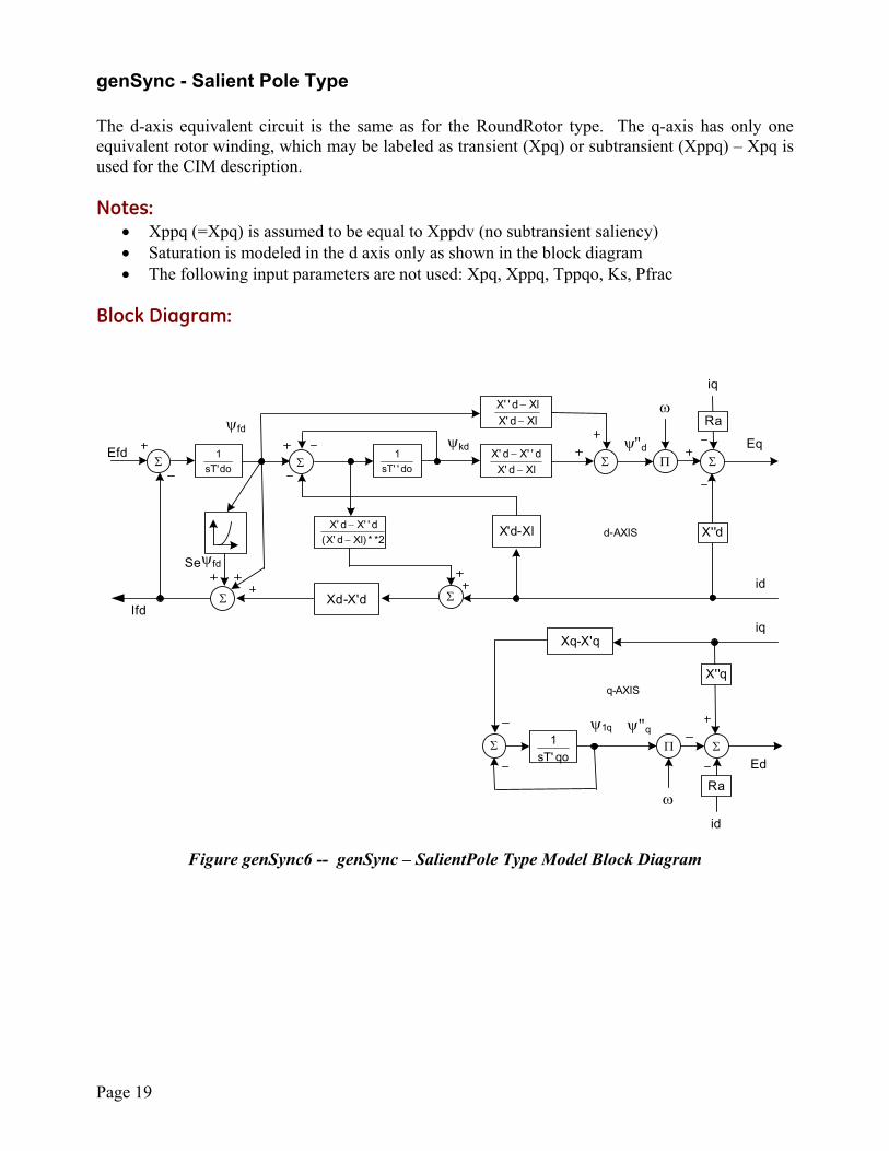
genSync - Salient Pole Type The d-axis equivalent circuit is the same as for the RoundRotor type. The q-axis has only one equivalent rotor winding, which may be labeled as transient (Xpq) or subtransient (Xppq) – Xpq is used for the CIM description. Notes:
• Xppq (=Xpq) is assumed to be equal to Xppdv (no subtransient saliency) • Saturation is modeled in the d axis only as shown in the block diagram • The following input parameters are not used: Xpq, Xppq, Tppqo, Ks, Pfrac
Block Diagram:
Se
do''sT1
2**)Xld'X(d''Xd'X
−− X'd-Xl d-AXIS
Efddo'sT
1Xld'X
d''Xd'X−
−
Xld'XXld''X
−−
Xd-X'dIfd
ψfdψkd
q-AXIS
iq
qo'sT1
Xq-X'q
ψ1q ψ"q
iq
id
X''d
Ra
Eq
id
Σ
X''q
Ra
Ed
ψ"dΠ
ω
Π
ω
Σ
Σ
Σ Σ
ΣΣ Σ
ψfd
Figure genSync6 -- genSync – SalientPole Type Model Block Diagram
Page 20
genSync - Transient Type The d-axis equivalent circuit has only the field winding. The q-axis has only one equivalent rotor winding, which may be labeled as transient (Xpq) or subtransient (Xppq) – Xpq is used for the CIM description. Notes:
• ??? Xppq (=Xpq) is assumed to be equal to Xppdv (=Xpd) (no subtransient saliency) • Saturation is modeled in the d axis only as shown in the block diagram • The following input parameters are not used: Xppd, Xpq, Xppq, Tpdo, Tppqo, Ks, Pfrac
Block Diagram: Add figure later
Figure genSync7 -- genSync – Transient Type Model Block Diagram
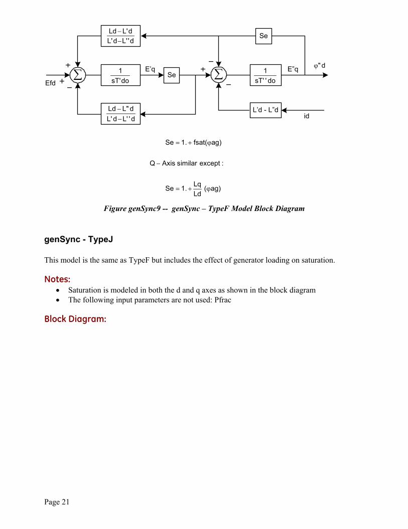
genSync - TypeF This model has a similar level of detail to the RoundRotor type but permits subtransient saliency (Xppq ≠ Xppdv) and models saturation differently. The RoundRotor type can usually be substituted without significant loss of accuracy. Notes:
• Saturation is modeled in both the d and q axes as shown in the block diagram • The following input parameters are not used: Ks, Pfrac
Block Diagram:
Page 21
do''sT1
id
Efd do'sT1
d''Ld'Ld'LLd
−−
L’d - L”dd''Ld'Ld"LLd
−−
E’q
Se
SeE”q
)ag(LdLq.1Se
:exceptsimilarAxisQ
)ag(fsat.1Se
ϕ+=
−
ϕ+=
d"ϕ∑∑
Figure genSync9 -- genSync – TypeF Model Block Diagram
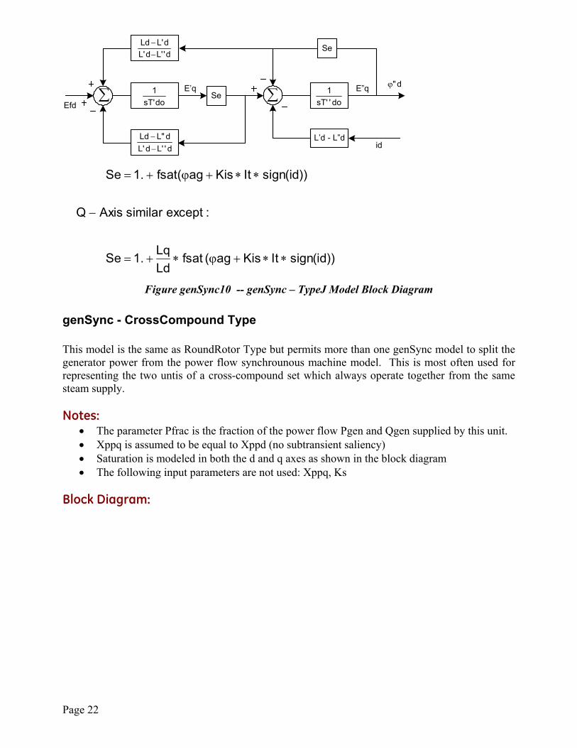
genSync - TypeJ This model is the same as TypeF but includes the effect of generator loading on saturation. Notes:
• Saturation is modeled in both the d and q axes as shown in the block diagram • The following input parameters are not used: Pfrac
Block Diagram:
Page 22
do''sT1
id
Efd do'sT1
d''Ld'Ld'LLd
−−
L’d - L”dd''Ld'Ld"LLd
−−
E’q
Se
SeE”q
))id(signItKisag(fsatLdLq.1Se
:exceptsimilarAxisQ
))id(signItKisag(fsat.1Se
∗∗+ϕ∗+=
−
∗∗+ϕ+=
d"ϕ
∑∑
Figure genSync10 -- genSync – TypeJ Model Block Diagram
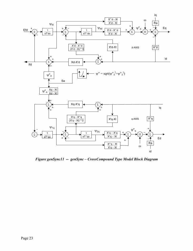
genSync - CrossCompound Type This model is the same as RoundRotor Type but permits more than one genSync model to split the generator power from the power flow synchrounous machine model. This is most often used for representing the two untis of a cross-compound set which always operate together from the same steam supply. Notes:
• The parameter Pfrac is the fraction of the power flow Pgen and Qgen supplied by this unit. • Xppq is assumed to be equal to Xppd (no subtransient saliency) • Saturation is modeled in both the d and q axes as shown in the block diagram • The following input parameters are not used: Xppq, Ks
Block Diagram:
Page 23
Se
XlXdXlXq
−−
ψ" = sqrt(ψ"d2+ψ"d
2)ψ"d
ψ"q
do''sT1
2**)Xld'X(d''Xd'X
−− X'd-Xl d-AXIS
Efddo'sT
1Xld'X
d''Xd'X−
−
Xld'XXld''X
−−
Xd-X'dIfd
ψfdψkd
qo''sT1
2**)Xlq'X(q''Xq'X
−−
X'q-Xl q-AXIS
iq
qo'sT1
Xlq'Xq'Xq'X
−−
Xlq'XXlq''X
−−
Xq-X'q
ψ1qψ2q
ψ"q
iq
id
X''d
Ra
Eq
id
Σ
X''q
Ra
Ed
ψ"dΠ
ω
Π
ω
ΣΣ
ΣΣ
Σ
Σ
Σ Σ
ΣΣ Σ
Figure genSync11 -- genSync – CrossCompound Type Model Block Diagram
Page 24
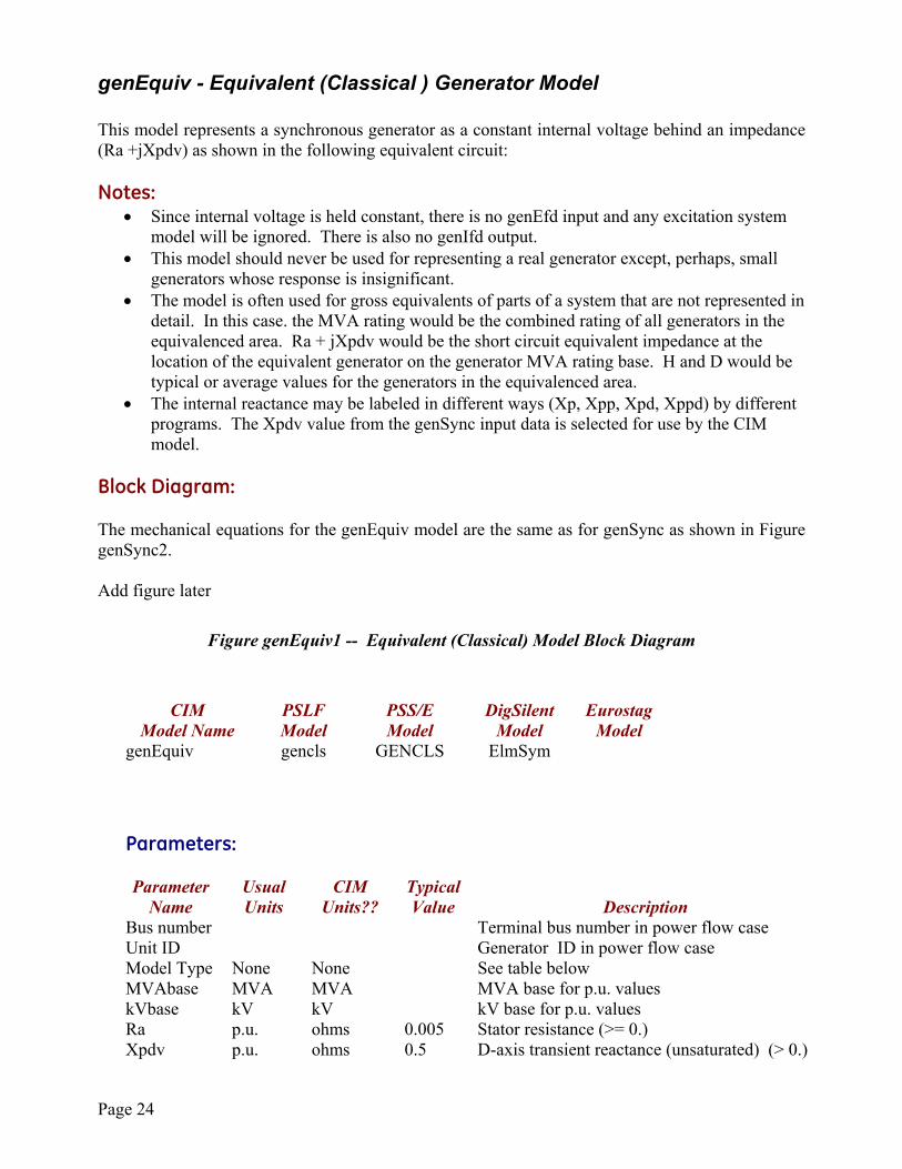
genEquiv - Equivalent (Classical ) Generator Model This model represents a synchronous generator as a constant internal voltage behind an impedance (Ra +jXpdv) as shown in the following equivalent circuit: Notes:
• Since internal voltage is held constant, there is no genEfd input and any excitation system model will be ignored. There is also no genIfd output.
• This model should never be used for representing a real generator except, perhaps, small generators whose response is insignificant.
• The model is often used for gross equivalents of parts of a system that are not represented in detail. In this case. the MVA rating would be the combined rating of all generators in the equivalenced area. Ra + jXpdv would be the short circuit equivalent impedance at the location of the equivalent generator on the generator MVA rating base. H and D would be typical or average values for the generators in the equivalenced area.
• The internal reactance may be labeled in different ways (Xp, Xpp, Xpd, Xppd) by different programs. The Xpdv value from the genSync input data is selected for use by the CIM model.
Block Diagram: The mechanical equations for the genEquiv model are the same as for genSync as shown in Figure genSync2. Add figure later
Figure genEquiv1 -- Equivalent (Classical) Model Block Diagram CIM PSLF PSS/E DigSilent Eurostag Model Name Model Model Model Model genEquiv gencls GENCLS ElmSym Parameters:
Parameter Usual CIM Typical Name Units Units?? Value Description Bus number Terminal bus number in power flow case Unit ID Generator ID in power flow case Model Type None None See table below MVAbase MVA MVA MVA base for p.u. values kVbase kV kV kV base for p.u. values Ra p.u. ohms 0.005 Stator resistance (>= 0.) Xpdv p.u. ohms 0.5 D-axis transient reactance (unsaturated) (> 0.)
Page 25
H sec.* MW-sec. 3.0 Inertia constant of turbine-generator (> 0.) D none** none 0.0 Damping factor
1. Parameter Xpd is actually used as an inductance (L) in the model, but is commonly referred
to as a reactance since, at nominal frequency, the per unit values are the same. However, some references (e.g. PSLF User Manual) use the symbol L instead of X. Also, the “p” in the parameter name is a substitution for a “prime” in the usual notation, e.g. Xpd refers to X’d.
2. H is the stored energy in the rotating mass of the generator plus all other elements (turbine, exciter) on the same shaft and has units of MW-sec. Conventional units are per unit on the generator MVA base, usually expressed as MW-sec./MVA or just sec. (since MW and MVA are equivalent units).
3. D has units of power/speed but is regarded as a dimensionless factor resulting from
linearization of an exponential relationship between speed and power: ( )DoPP ω= . This value is often zero when the source of damping torques (generator damper windings, load damping effects, etc.) are modeling in detail. [ref]
Page 26
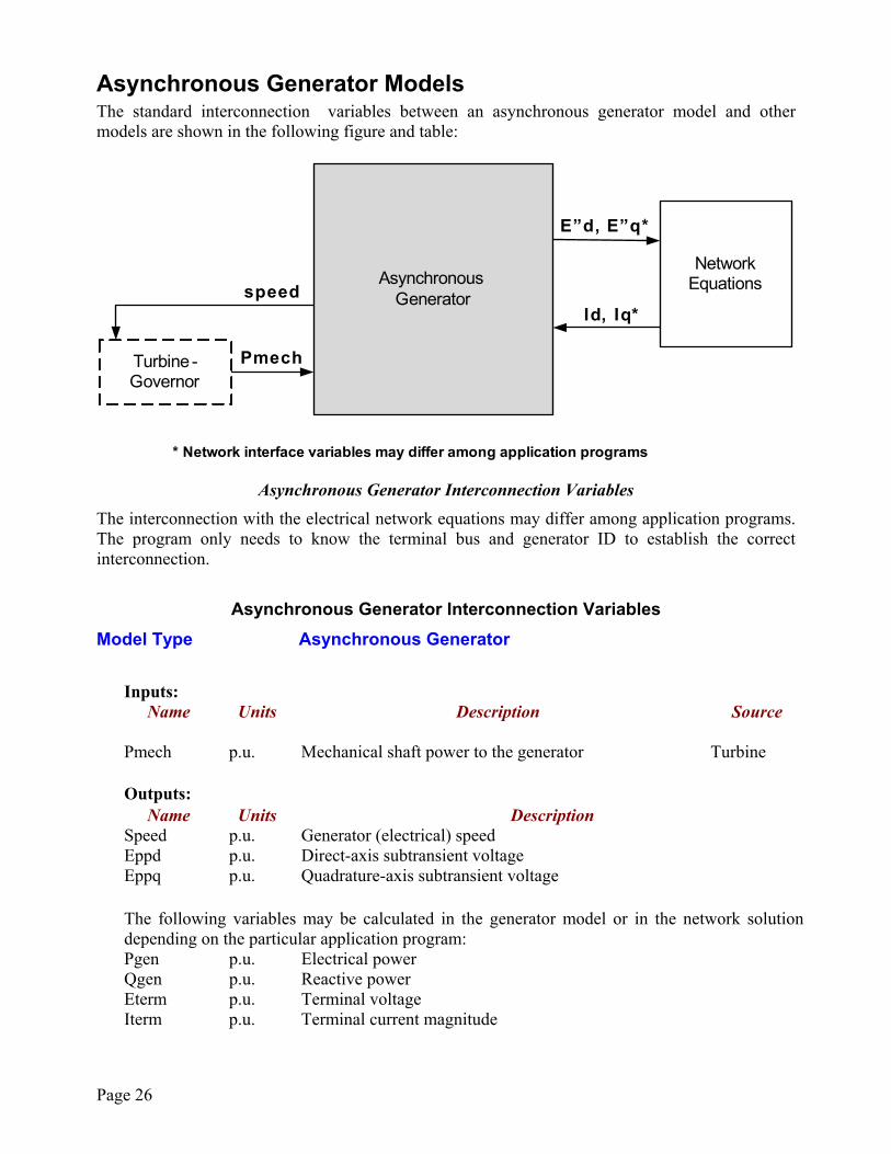
Asynchronous Generator Models The standard interconnection variables between an asynchronous generator model and other models are shown in the following figure and table:
AsynchronousGenerator
Pmech
Network Equations
Turbine -Governor
speedId, Iq*
E”d, E”q*
* Network interface variables may differ among application programs
Asynchronous Generator Interconnection Variables The interconnection with the electrical network equations may differ among application programs. The program only needs to know the terminal bus and generator ID to establish the correct interconnection.
Asynchronous Generator Interconnection Variables
Model Type Asynchronous Generator
Inputs: Name
Units Description Source
Pmech p.u. Mechanical shaft power to the generator Turbine Outputs: Name Units Description Speed p.u. Generator (electrical) speed Eppd p.u. Direct-axis subtransient voltage Eppq p.u. Quadrature-axis subtransient voltage The following variables may be calculated in the generator model or in the network solution
depending on the particular application program: Pgen p.u. Electrical power Qgen p.u. Reactive power Eterm p.u. Terminal voltage Iterm p.u. Terminal current magnitude
Page 27
Initialization Inputs: Name
Units Description Source
Eterm p.u. Terminal voltage magnitude Power Flow busAngle radians Terminal voltage angle relative to system reference Power Flow Pgen MW Electrical power Power Flow Qgen MVAr Reactive power Power Flow Initialization Outputs: Name Units Description Speed p.u. Generator (electrical) speed (= 1.0 initially) Pmech p.u. Mechanical shaft power to the generator Notes:
1. Input/output variable units should be kept in per unit. Attempts to convert to engineering units would be confusing. Since these variable are not directly attributes of CIM classes, this should not conflict with CIM standards.
2. The interface between the generator model and the network algebraic equations is
application dependent. The variables used for this interface do not need to be specified since they are internal to the application program and will not be used by other models, e.g. user-written models.
3. If no Turbine-Governor model is present for a unit, the generator mechanical power
(Pmech) should be held constant at the initial value.
Page 28
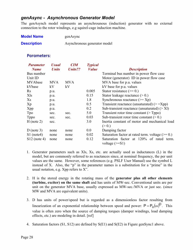
genAsync - Asynchronous Generator Model The genAsynch model represents an asynchrounous (induction) generator with no external connection to the rotor windings, e.g squirel-cage induction machine. Model Name genAsync
Description Asynchronous generator model
Parameters:
Parameter Usual CIM Typical Name Units Units?? Value Description Bus number Terminal bus number in power flow case Unit ID Motor (generator) ID in power flow case MVAbase MVA MVA MVA base for p.u. values kVbase kV kV kV base for p.u. values Rs p.u. 0.005 Stator resistance (>= 0.) Xls p.u. 0.15 Stator leakage reactance (> 0.) Xs p.u. 1.8 Synchronous reactance (>= Xp) Xp p.u. 0.5 Transient reactance (unsaturated) (> =Xpp) Xpp p.u. 0.2 Sub-transient reactance (unsaturated) (> Xl) Tpo sec. sec. 5.0 Transient rotor time constant (> Tppo) Tppo sec. sec. 0.03 Sub-transient rotor time constant (> 0.) H (note 2) sec. 3.0 Inertia constant of motor and mechanical load
(> 0.) D (note 3) none none 0.0 Damping factor S1 (note4) none none 0.02 Saturation factor at rated term. voltage (>= 0.) S12 (note 4) none none 0.12 Saturation factor at 120% of rated term.
voltage (>=S1)
1. Generator parameters such as Xls, Xs, etc. are actually used as inductances (L) in the model, but are commonly referred to as reactances since, at nominal frequency, the per unit values are the same. However, some references (e.g. PSLF User Manual) use the symbol L instead of X. Also, the “p” in the parameter names is a substitution for a “prime” in the usual notation, e.g. Xpp refers to X”.
2. H is the stored energy in the rotating mass of the generator plus all other elements (turbine, exciter) on the same shaft and has units of MW-sec. Conventional units are per unit on the generator MVA base, usually expressed as MW-sec./MVA or just sec. (since MW and MVA are equivalent units).
3. D has units of power/speed but is regarded as a dimensionless factor resulting from
linearization of an exponential relationship between speed and power: ( )DoPP ω= . This value is often zero when the source of damping torques (damper windings, load damping effects, etc.) are modeling in detail. [ref]
4. Saturation factors (S1, S12) are defined by S(E1) and S(E2) in Figure genSync1 above.
Page 29
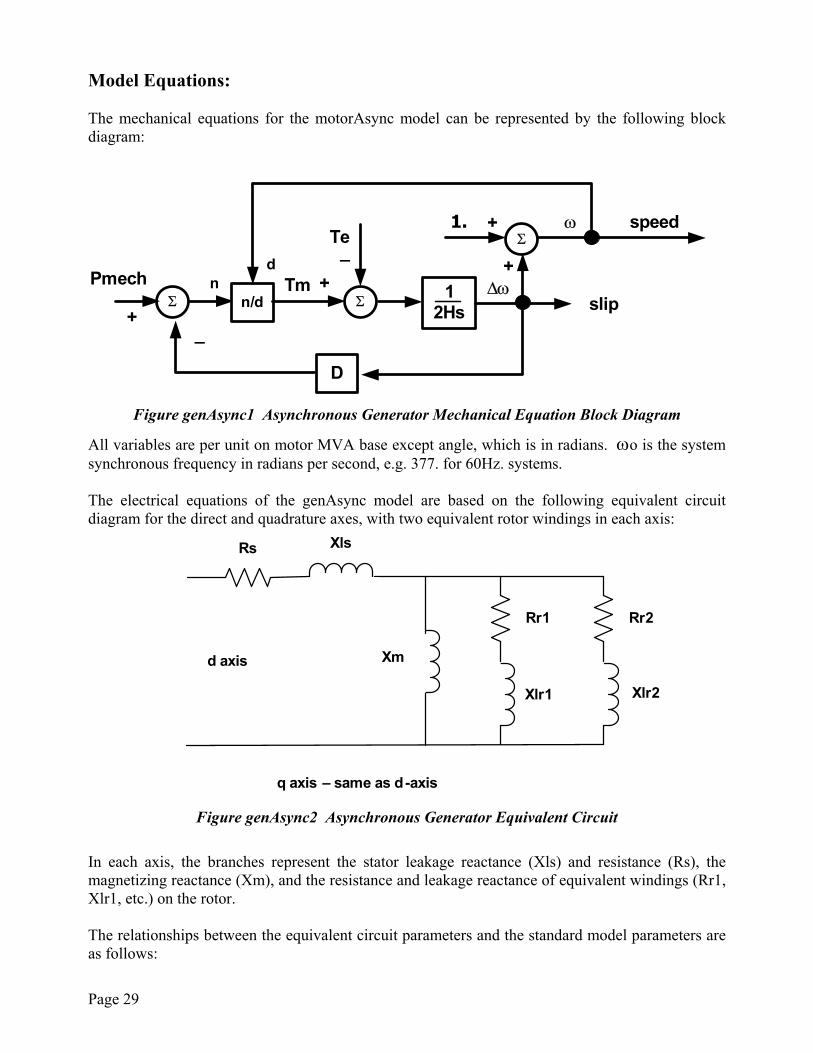
Model Equations: The mechanical equations for the motorAsync model can be represented by the following block diagram:
12Hs
∆ω
D
Tespeed
Pmech
1. +
+
Σ+
_ω
n/dn Tm
d
Σ
Σ
slip_
+
Figure genAsync1 Asynchronous Generator Mechanical Equation Block Diagram
All variables are per unit on motor MVA base except angle, which is in radians. ωo is the system synchronous frequency in radians per second, e.g. 377. for 60Hz. systems. The electrical equations of the genAsync model are based on the following equivalent circuit diagram for the direct and quadrature axes, with two equivalent rotor windings in each axis:
Xls
Xlr2Xlr1
Xm
Rr1
Rs
Rr2
d axis
q axis – same as d-axis
Figure genAsync2 Asynchronous Generator Equivalent Circuit In each axis, the branches represent the stator leakage reactance (Xls) and resistance (Rs), the magnetizing reactance (Xm), and the resistance and leakage reactance of equivalent windings (Rr1, Xlr1, etc.) on the rotor. The relationships between the equivalent circuit parameters and the standard model parameters are as follows:
Page 30
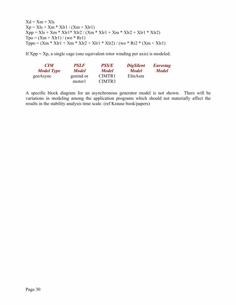
Xd = Xm + Xls Xp = Xls + Xm * Xlr1 / (Xm + Xlr1) Xpp = Xls + Xm * Xlr1* Xlr2 / (Xm * Xlr1 + Xm * Xlr2 + Xlr1 * Xlr2) Tpo = (Xm + Xlr1) / (wo * Rr1) Tppo = (Xm * Xlr1 + Xm * Xlr2 + Xlr1 * Xlr2) / (wo * Rr2 * (Xm + Xlr1) If Xpp = Xp, a single cage (one equivalent rotor winding per axis) is modeled. CIM PSLF PSS/E DigSilent Eurostag Model Type Model Model Model Model genAsync genind or
motor1 CIMTR1 CIMTR3
ElmAsm
A specific block diagram for an asynchronous generator model is not shown. There will be variations in modeling among the application programs which should not materially affect the results in the stability analysis time scale. (ref Krause book/papers)
Page 31
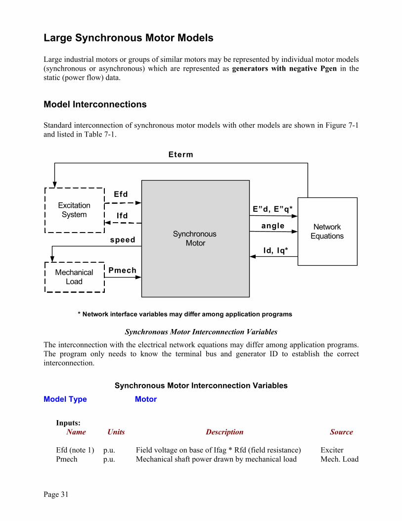
Large Synchronous Motor Models Large industrial motors or groups of similar motors may be represented by individual motor models (synchronous or asynchronous) which are represented as generators with negative Pgen in the static (power flow) data.
Model Interconnections Standard interconnection of synchronous motor models with other models are shown in Figure 7-1 and listed in Table 7-1.
Efd
Synchronous Motor
Pmech
Network Equations
Mechanical Load
Excitation System I fd
speed
Eterm
Id, Iq*
E”d, E”q*
* Network interface variables may differ among application programs
angle
Synchronous Motor Interconnection Variables
The interconnection with the electrical network equations may differ among application programs. The program only needs to know the terminal bus and generator ID to establish the correct interconnection.
Synchronous Motor Interconnection Variables
Model Type Motor
Inputs: Name
Units Description Source
Efd (note 1) p.u. Field voltage on base of Ifag * Rfd (field resistance) Exciter Pmech p.u. Mechanical shaft power drawn by mechanical load Mech. Load
Page 32
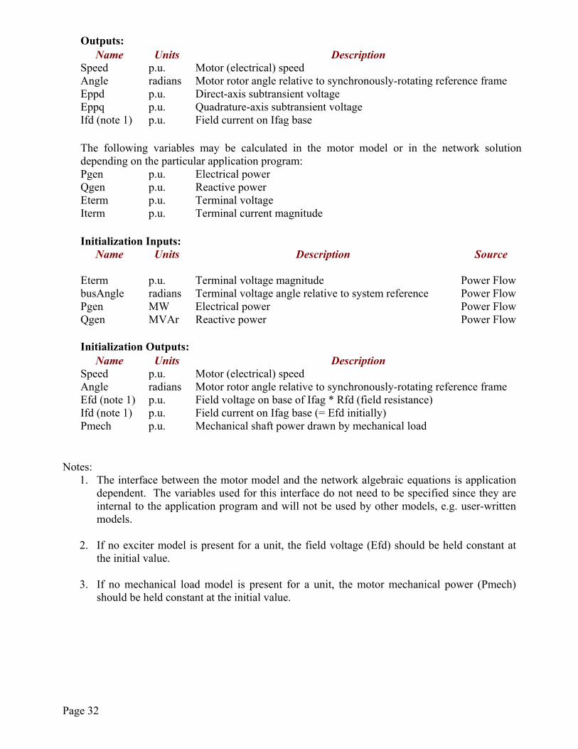
Outputs: Name Units Description Speed p.u. Motor (electrical) speed Angle radians Motor rotor angle relative to synchronously-rotating reference frame Eppd p.u. Direct-axis subtransient voltage Eppq p.u. Quadrature-axis subtransient voltage Ifd (note 1) p.u. Field current on Ifag base The following variables may be calculated in the motor model or in the network solution
depending on the particular application program: Pgen p.u. Electrical power Qgen p.u. Reactive power Eterm p.u. Terminal voltage Iterm p.u. Terminal current magnitude Initialization Inputs: Name
Units Description Source
Eterm p.u. Terminal voltage magnitude Power Flow busAngle radians Terminal voltage angle relative to system reference Power Flow Pgen MW Electrical power Power Flow Qgen MVAr Reactive power Power Flow Initialization Outputs: Name Units Description Speed p.u. Motor (electrical) speed Angle radians Motor rotor angle relative to synchronously-rotating reference frame Efd (note 1) p.u. Field voltage on base of Ifag * Rfd (field resistance) Ifd (note 1) p.u. Field current on Ifag base (= Efd initially) Pmech p.u. Mechanical shaft power drawn by mechanical load Notes:
1. The interface between the motor model and the network algebraic equations is application dependent. The variables used for this interface do not need to be specified since they are internal to the application program and will not be used by other models, e.g. user-written models.
2. If no exciter model is present for a unit, the field voltage (Efd) should be held constant at
the initial value.
3. If no mechanical load model is present for a unit, the motor mechanical power (Pmech) should be held constant at the initial value.
Page 33
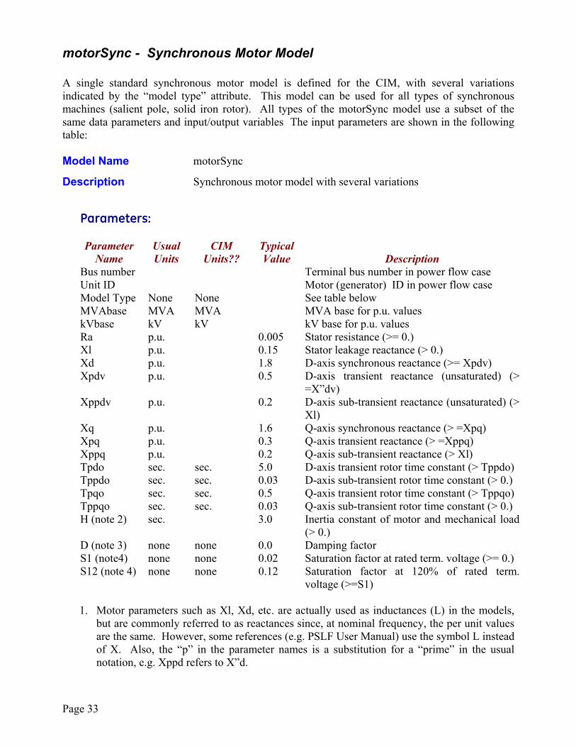
motorSync - Synchronous Motor Model A single standard synchronous motor model is defined for the CIM, with several variations indicated by the “model type” attribute. This model can be used for all types of synchronous machines (salient pole, solid iron rotor). All types of the motorSync model use a subset of the same data parameters and input/output variables The input parameters are shown in the following table: Model Name motorSync
Description Synchronous motor model with several variations
Parameters:
Parameter Usual CIM Typical Name Units Units?? Value Description Bus number Terminal bus number in power flow case Unit ID Motor (generator) ID in power flow case Model Type None None See table below MVAbase MVA MVA MVA base for p.u. values kVbase kV kV kV base for p.u. values Ra p.u. 0.005 Stator resistance (>= 0.) Xl p.u. 0.15 Stator leakage reactance (> 0.) Xd p.u. 1.8 D-axis synchronous reactance (>= Xpdv) Xpdv p.u. 0.5 D-axis transient reactance (unsaturated) (>
=X”dv) Xppdv p.u. 0.2 D-axis sub-transient reactance (unsaturated) (>
Xl) Xq p.u. 1.6 Q-axis synchronous reactance (> =Xpq) Xpq p.u. 0.3 Q-axis transient reactance (> =Xppq) Xppq p.u. 0.2 Q-axis sub-transient reactance (> Xl) Tpdo sec. sec. 5.0 D-axis transient rotor time constant (> Tppdo) Tppdo sec. sec. 0.03 D-axis sub-transient rotor time constant (> 0.) Tpqo sec. sec. 0.5 Q-axis transient rotor time constant (> Tppqo) Tppqo sec. sec. 0.03 Q-axis sub-transient rotor time constant (> 0.) H (note 2) sec. 3.0 Inertia constant of motor and mechanical load
(> 0.) D (note 3) none none 0.0 Damping factor S1 (note4) none none 0.02 Saturation factor at rated term. voltage (>= 0.) S12 (note 4) none none 0.12 Saturation factor at 120% of rated term.
voltage (>=S1)
1. Motor parameters such as Xl, Xd, etc. are actually used as inductances (L) in the models, but are commonly referred to as reactances since, at nominal frequency, the per unit values are the same. However, some references (e.g. PSLF User Manual) use the symbol L instead of X. Also, the “p” in the parameter names is a substitution for a “prime” in the usual notation, e.g. Xppd refers to X”d.
Page 34
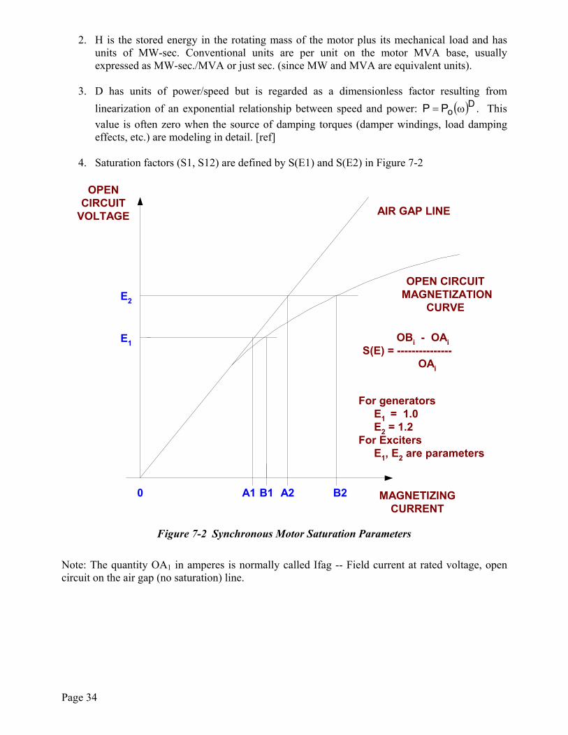
2. H is the stored energy in the rotating mass of the motor plus its mechanical load and has units of MW-sec. Conventional units are per unit on the motor MVA base, usually expressed as MW-sec./MVA or just sec. (since MW and MVA are equivalent units).
3. D has units of power/speed but is regarded as a dimensionless factor resulting from
linearization of an exponential relationship between speed and power: ( )DoPP ω= . This value is often zero when the source of damping torques (damper windings, load damping effects, etc.) are modeling in detail. [ref]
4. Saturation factors (S1, S12) are defined by S(E1) and S(E2) in Figure 7-2
E1
OPENCIRCUIT
VOLTAGE
OPEN CIRCUIT MAGNETIZATION
CURVE
MAGNETIZINGCURRENT
For generators E1 = 1.0 E2 = 1.2For Exciters E1, E2 are parameters
E2
A1 B1 A2 B2
AIR GAP LINE
0
OBi - OAi S(E) = --------------- OAi
Figure 7-2 Synchronous Motor Saturation Parameters
Note: The quantity OA1 in amperes is normally called Ifag -- Field current at rated voltage, open circuit on the air gap (no saturation) line.
Page 35
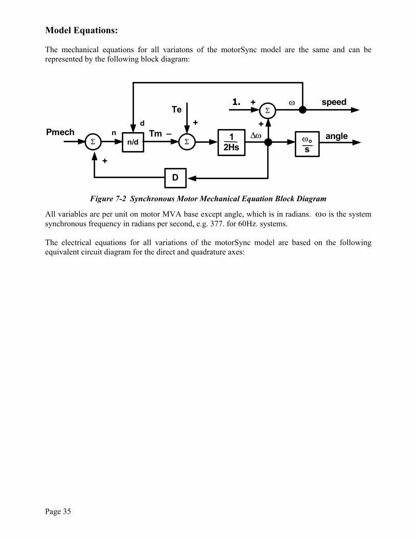
Model Equations: The mechanical equations for all variatons of the motorSync model are the same and can be represented by the following block diagram:
12Hs
∆ω
D
Tespeed
anglePmech
1. +
ωos
+
Σ
+_
ω
n/dn Tm
d
Σ
Σ
+
Figure 7-2 Synchronous Motor Mechanical Equation Block Diagram
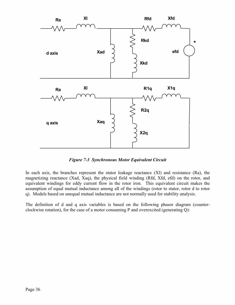
All variables are per unit on motor MVA base except angle, which is in radians. ωo is the system synchronous frequency in radians per second, e.g. 377. for 60Hz. systems. The electrical equations for all variations of the motorSync model are based on the following equivalent circuit diagram for the direct and quadrature axes:
Page 36
+
efd
Xl Xfd
Xkd
Xad
Rkd
Ra Rfd
d axis
Xl X1q
X2q
Xaq
R2q
Ra R1q
q axis
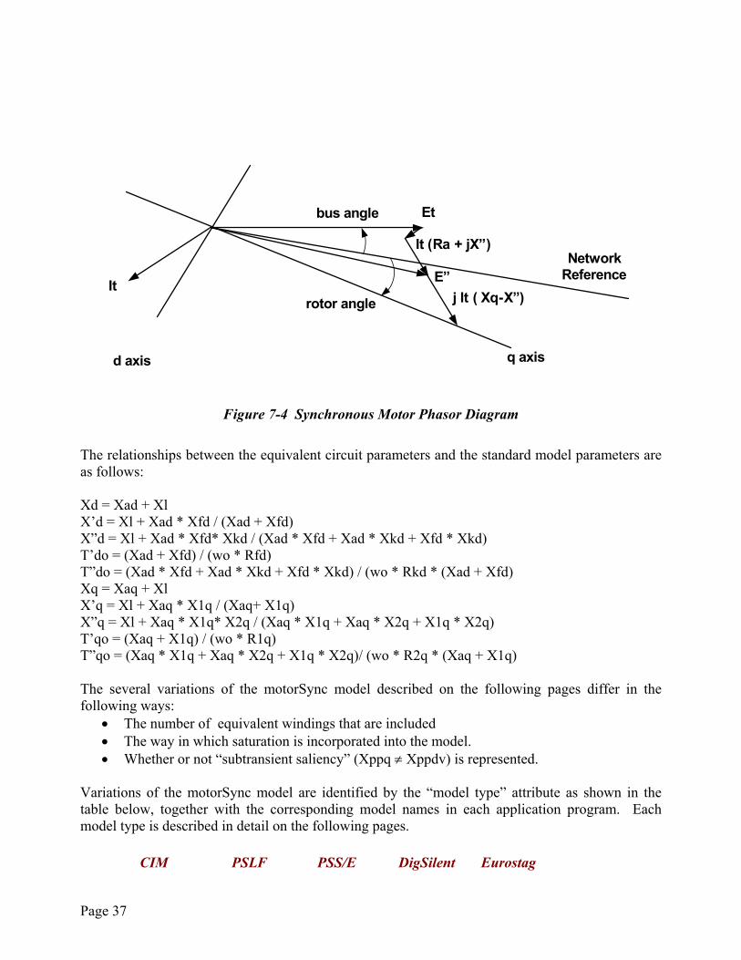
Figure 7-3 Synchronous Motor Equivalent Circuit In each axis, the branches represent the stator leakage reactance (Xl) and resistance (Ra), the magnetizing reactance (Xad, Xaq), the physical field winding (Rfd, Xfd, efd) on the rotor, and equivalent windings for eddy current flow in the rotor iron. This equivalent circuit makes the assumption of equal mutual inductance among all of the windings (rotor to stator, rotor d to rotor q). Models based on unequal mutual inductance are not normally used for stability analysis. The definition of d and q axis variables is based on the following phasor diagram (counter-clockwise rotation), for the case of a motor consuming P and overexcited (generating Q):
Page 37
q axis
Et
It
It (Ra + jX”)
E”j It ( Xq-X”)
d axis
Network Reference
rotor angle
bus angle
Figure 7-4 Synchronous Motor Phasor Diagram
The relationships between the equivalent circuit parameters and the standard model parameters are as follows: Xd = Xad + Xl X’d = Xl + Xad * Xfd / (Xad + Xfd) X”d = Xl + Xad * Xfd* Xkd / (Xad * Xfd + Xad * Xkd + Xfd * Xkd) T’do = (Xad + Xfd) / (wo * Rfd) T”do = (Xad * Xfd + Xad * Xkd + Xfd * Xkd) / (wo * Rkd * (Xad + Xfd) Xq = Xaq + Xl X’q = Xl + Xaq * X1q / (Xaq+ X1q) X”q = Xl + Xaq * X1q* X2q / (Xaq * X1q + Xaq * X2q + X1q * X2q) T’qo = (Xaq + X1q) / (wo * R1q) T”qo = (Xaq * X1q + Xaq * X2q + X1q * X2q)/ (wo * R2q * (Xaq + X1q) The several variations of the motorSync model described on the following pages differ in the following ways:
• The number of equivalent windings that are included • The way in which saturation is incorporated into the model. • Whether or not “subtransient saliency” (Xppq ≠ Xppdv) is represented.
Variations of the motorSync model are identified by the “model type” attribute as shown in the table below, together with the corresponding model names in each application program. Each model type is described in detail on the following pages. CIM PSLF PSS/E DigSilent Eurostag
Page 38
Model Type Model Model Model Model RoundRotor genrou GENROU ElmSym SalientPole gensal GENSAL ElmSym Note: It is not necessary for each program to have separate models for each of the model types. The same model can often be used for several types by alternative logic within the model. Also, differences in saturation representation may not result in significant model performance differences so model substitutions are often acceptable.
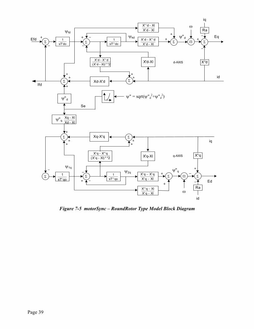
motorSync - RoundRotor Type The complete equivalent circuit is used with two rotor windings in each axis. Notes:
• Xppq is assumed to be equal to Xppd (no subtransient saliency) • Saturation is modeled in both the d and q axes as shown in the block diagram • The following input parameters are not used: Xppq
Block Diagram:
Page 39
Se
XlXdXlXq
−−
ψ" = sqrt(ψ"d2+ψ"d
2)ψ"d
ψ"q
do''sT1
2**)Xld'X(d''Xd'X
−− X'd-Xl d-AXIS
Efddo'sT
1Xld'X
d''Xd'X−
−
Xld'XXld''X
−−
Xd-X'dIfd
ψfdψkd
qo''sT1
2**)Xlq'X(q''Xq'X
−−
X'q-Xl q-AXIS
iq
qo'sT1
Xlq'Xq'Xq'X
−−
Xlq'XXlq''X
−−
Xq-X'q
ψ1qψ2q
ψ"q
iq
id
X''d
Ra
Eq
id
Σ
X''q
Ra
Ed
ψ"dΠ
ω
Π
ω
ΣΣ
ΣΣ
Σ
Σ
Σ Σ
ΣΣ Σ
Figure 7-5 motorSync – RoundRotor Type Model Block Diagram
Page 40
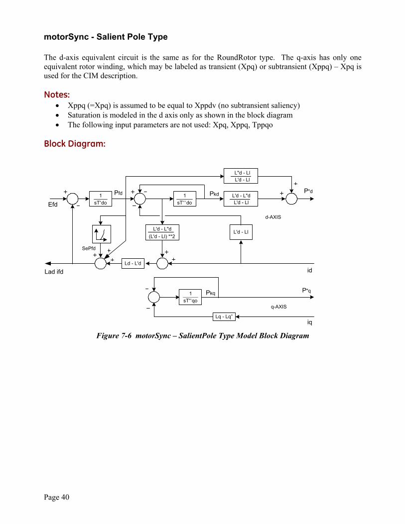
motorSync - Salient Pole Type The d-axis equivalent circuit is the same as for the RoundRotor type. The q-axis has only one equivalent rotor winding, which may be labeled as transient (Xpq) or subtransient (Xppq) – Xpq is used for the CIM description. Notes:
• Xppq (=Xpq) is assumed to be equal to Xppdv (no subtransient saliency) • Saturation is modeled in the d axis only as shown in the block diagram • The following input parameters are not used: Xpq, Xppq, Tppqo
Block Diagram:
do''sT1
L'd - Ll
d-AXIS
id
Efd do'sT1
q-AXIS
iq
Pfd
Ld - L'd
qo''sT1
Lq - Lq”
L"d - LlL'd - Ll
L'd - L"dL'd - Ll
L'd - L"d(L'd - Ll) **2
SePfd
Lad ifd
Pkd
Pkq
P"d
P"q
Figure 7-6 motorSync – SalientPole Type Model Block Diagram
Page 41
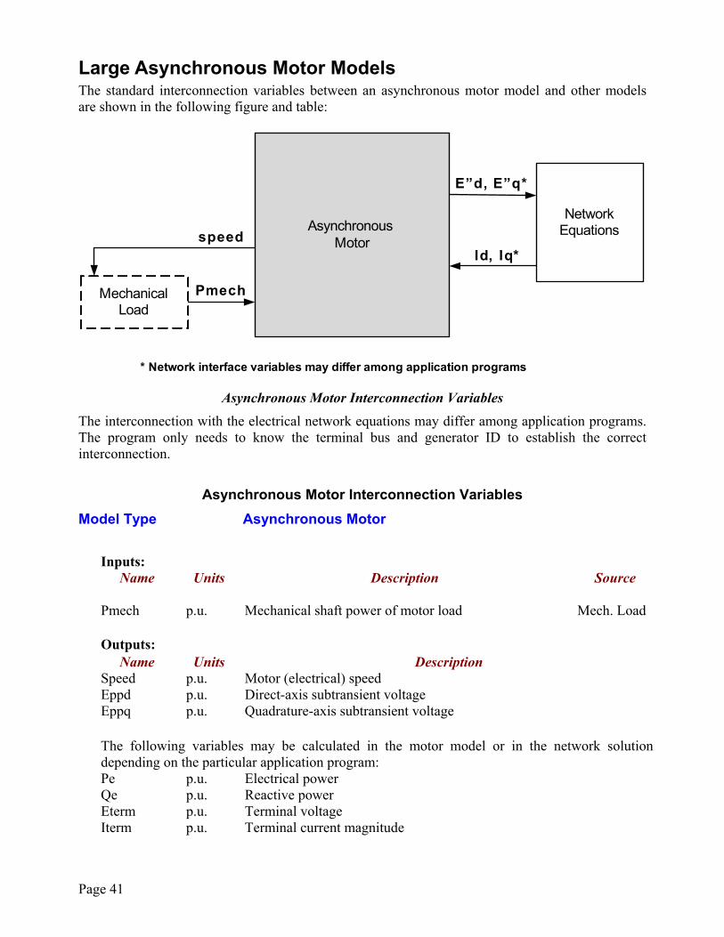
Large Asynchronous Motor Models The standard interconnection variables between an asynchronous motor model and other models are shown in the following figure and table:
AsynchronousMotor
Pmech
Network Equations
Mechanical Load
speedId, Iq*
E”d, E”q*
* Network interface variables may differ among application programs
Asynchronous Motor Interconnection Variables The interconnection with the electrical network equations may differ among application programs. The program only needs to know the terminal bus and generator ID to establish the correct interconnection.
Asynchronous Motor Interconnection Variables
Model Type Asynchronous Motor
Inputs: Name
Units Description Source
Pmech p.u. Mechanical shaft power of motor load Mech. Load Outputs: Name Units Description Speed p.u. Motor (electrical) speed Eppd p.u. Direct-axis subtransient voltage Eppq p.u. Quadrature-axis subtransient voltage The following variables may be calculated in the motor model or in the network solution
depending on the particular application program: Pe p.u. Electrical power Qe p.u. Reactive power Eterm p.u. Terminal voltage Iterm p.u. Terminal current magnitude
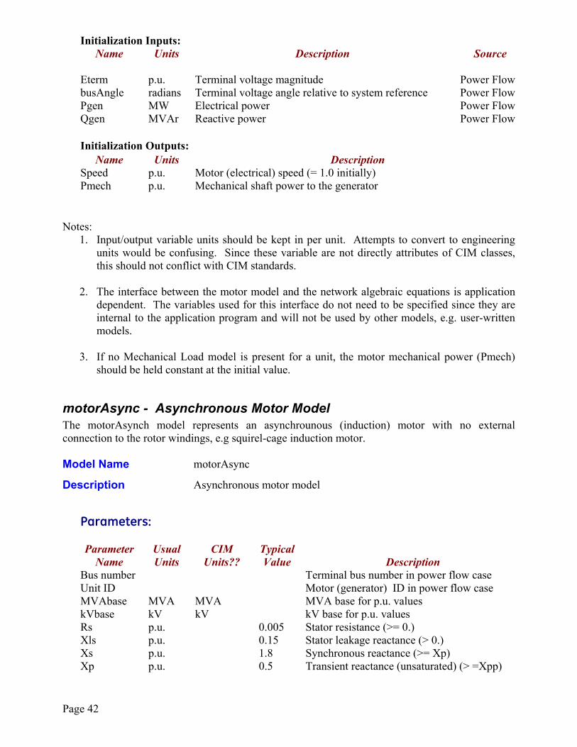
Page 42
Initialization Inputs: Name
Units Description Source
Eterm p.u. Terminal voltage magnitude Power Flow busAngle radians Terminal voltage angle relative to system reference Power Flow Pgen MW Electrical power Power Flow Qgen MVAr Reactive power Power Flow Initialization Outputs: Name Units Description Speed p.u. Motor (electrical) speed (= 1.0 initially) Pmech p.u. Mechanical shaft power to the generator Notes:
1. Input/output variable units should be kept in per unit. Attempts to convert to engineering units would be confusing. Since these variable are not directly attributes of CIM classes, this should not conflict with CIM standards.
2. The interface between the motor model and the network algebraic equations is application
dependent. The variables used for this interface do not need to be specified since they are internal to the application program and will not be used by other models, e.g. user-written models.
3. If no Mechanical Load model is present for a unit, the motor mechanical power (Pmech)
should be held constant at the initial value.
motorAsync - Asynchronous Motor Model The motorAsynch model represents an asynchrounous (induction) motor with no external connection to the rotor windings, e.g squirel-cage induction motor. Model Name motorAsync
Description Asynchronous motor model
Parameters:
Parameter Usual CIM Typical Name Units Units?? Value Description Bus number Terminal bus number in power flow case Unit ID Motor (generator) ID in power flow case MVAbase MVA MVA MVA base for p.u. values kVbase kV kV kV base for p.u. values Rs p.u. 0.005 Stator resistance (>= 0.) Xls p.u. 0.15 Stator leakage reactance (> 0.) Xs p.u. 1.8 Synchronous reactance (>= Xp) Xp p.u. 0.5 Transient reactance (unsaturated) (> =Xpp)
Page 43
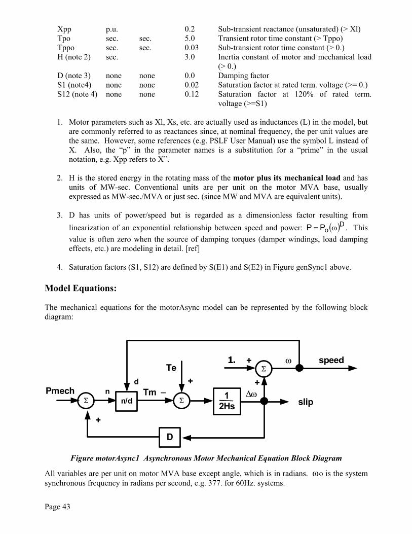
Xpp p.u. 0.2 Sub-transient reactance (unsaturated) (> Xl) Tpo sec. sec. 5.0 Transient rotor time constant (> Tppo) Tppo sec. sec. 0.03 Sub-transient rotor time constant (> 0.) H (note 2) sec. 3.0 Inertia constant of motor and mechanical load
(> 0.) D (note 3) none none 0.0 Damping factor S1 (note4) none none 0.02 Saturation factor at rated term. voltage (>= 0.) S12 (note 4) none none 0.12 Saturation factor at 120% of rated term.
voltage (>=S1)
1. Motor parameters such as Xl, Xs, etc. are actually used as inductances (L) in the model, but are commonly referred to as reactances since, at nominal frequency, the per unit values are the same. However, some references (e.g. PSLF User Manual) use the symbol L instead of X. Also, the “p” in the parameter names is a substitution for a “prime” in the usual notation, e.g. Xpp refers to X”.
2. H is the stored energy in the rotating mass of the motor plus its mechanical load and has units of MW-sec. Conventional units are per unit on the motor MVA base, usually expressed as MW-sec./MVA or just sec. (since MW and MVA are equivalent units).
3. D has units of power/speed but is regarded as a dimensionless factor resulting from
linearization of an exponential relationship between speed and power: ( )DoPP ω= . This value is often zero when the source of damping torques (damper windings, load damping effects, etc.) are modeling in detail. [ref]
4. Saturation factors (S1, S12) are defined by S(E1) and S(E2) in Figure genSync1 above.
Model Equations: The mechanical equations for the motorAsync model can be represented by the following block diagram:
12Hs
∆ω
D
Tespeed
Pmech
1. +
+
Σ
+_
ω
n/dn Tm
d
Σ
Σ
+
slip
Figure motorAsync1 Asynchronous Motor Mechanical Equation Block Diagram
All variables are per unit on motor MVA base except angle, which is in radians. ωo is the system synchronous frequency in radians per second, e.g. 377. for 60Hz. systems.
Page 44
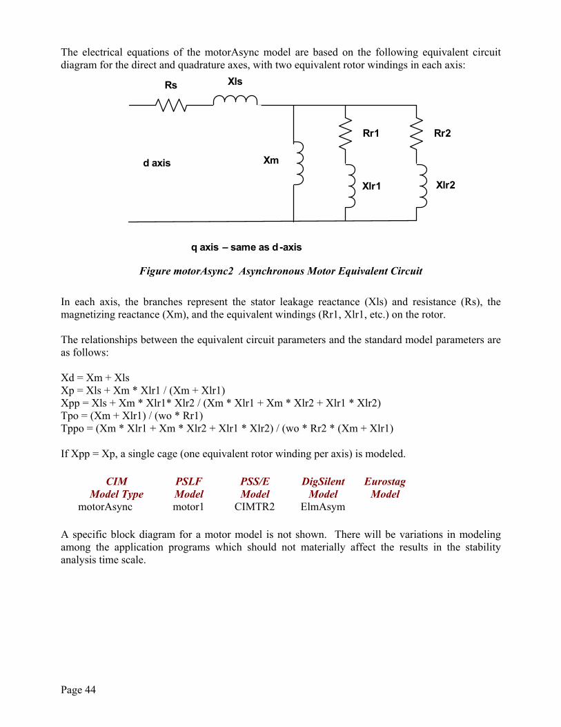
The electrical equations of the motorAsync model are based on the following equivalent circuit diagram for the direct and quadrature axes, with two equivalent rotor windings in each axis:
Xls
Xlr2Xlr1
Xm
Rr1
Rs
Rr2
d axis
q axis – same as d-axis
Figure motorAsync2 Asynchronous Motor Equivalent Circuit In each axis, the branches represent the stator leakage reactance (Xls) and resistance (Rs), the magnetizing reactance (Xm), and the equivalent windings (Rr1, Xlr1, etc.) on the rotor. The relationships between the equivalent circuit parameters and the standard model parameters are as follows: Xd = Xm + Xls Xp = Xls + Xm * Xlr1 / (Xm + Xlr1) Xpp = Xls + Xm * Xlr1* Xlr2 / (Xm * Xlr1 + Xm * Xlr2 + Xlr1 * Xlr2) Tpo = (Xm + Xlr1) / (wo * Rr1) Tppo = (Xm * Xlr1 + Xm * Xlr2 + Xlr1 * Xlr2) / (wo * Rr2 * (Xm + Xlr1) If Xpp = Xp, a single cage (one equivalent rotor winding per axis) is modeled. CIM PSLF PSS/E DigSilent Eurostag Model Type Model Model Model Model motorAsync motor1 CIMTR2 ElmAsym A specific block diagram for a motor model is not shown. There will be variations in modeling among the application programs which should not materially affect the results in the stability analysis time scale.
Page 45
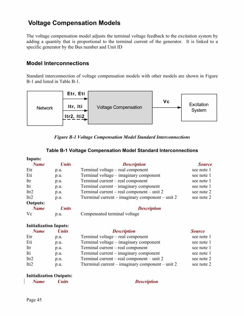
Voltage Compensation Models The voltage compensation model adjusts the terminal voltage feedback to the excitation system by adding a quantity that is proportional to the terminal current of the generator. It is linked to a specific generator by the Bus number and Unit ID
Model Interconnections Standard interconnection of voltage compensation models with other models are shown in Figure B-1 and listed in Table B-1.
VcEtr, Eti
Voltage Compensation Excitation System
Itr, It iNetwork
Itr2, Iti2
Figure B-1 Voltage Compensation Model Standard Interconnections
Table B-1 Voltage Compensation Model Standard Interconnections Inputs:
Name Units Description Source Etr p.u. Terminal voltage – real component see note 1 Eti p.u. Terminal voltage – imaginary component see note 1 Itr p.u. Terminal current – real component see note 1 Iti p.u. Terminal current – imaginary component see note 1 Itr2 p.u. Terminal current – real component – unit 2 see note 2 Iti2 p.u. Tterminal current – imaginary component – unit 2 see note 2 Outputs:
Name Units Description Vc p.u. Compensated terminal voltage Initialization Inputs:
Name Units Description Source Etr p.u. Terminal voltage – real component see note 1 Eti p.u. Terminal voltage – imaginary component see note 1 Itr p.u. Terminal current – real component see note 1 Iti p.u. Terminal current – imaginary component see note 1 Itr2 p.u. Terminal current – real component – unit 2 see note 2 Iti2 p.u. Tterminal current – imaginary component – unit 2 see note 2 Initialization Outputs:
Name Units Description
Page 46
Vc p.u. Compensated terminal voltage Notes: 1. Source of the generator complex voltage components is application dependent. It may come
from the generator or from the network equations. 2. Unit 2 is a second generator connected to the same terminal bus, usually the other unit of a
cross-compound pair. These inputs are not used by all voltage compensation models.
Page 47
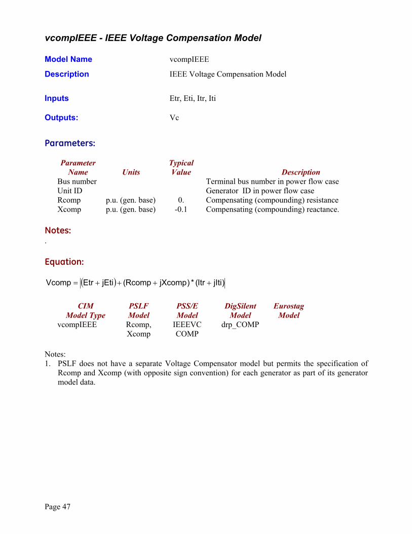
vcompIEEE - IEEE Voltage Compensation Model Model Name vcompIEEE
Description IEEE Voltage Compensation Model
Inputs Etr, Eti, Itr, Iti Outputs: Vc
Parameters:
Parameter Typical Name Units Value Description Bus number Terminal bus number in power flow case Unit ID Generator ID in power flow case Rcomp p.u. (gen. base) 0. Compensating (compounding) resistance Xcomp p.u. (gen. base) -0.1 Compensating (compounding) reactance. Notes: . Equation:
( ) )jItiItr(*)jXcompRcomp(jEtiEtrVcomp ++++=
CIM PSLF PSS/E DigSilent Eurostag Model Type Model Model Model Model vcompIEEE Rcomp,
Xcomp IEEEVC COMP
drp_COMP
Notes: 1. PSLF does not have a separate Voltage Compensator model but permits the specification of
Rcomp and Xcomp (with opposite sign convention) for each generator as part of its generator model data.
Page 48
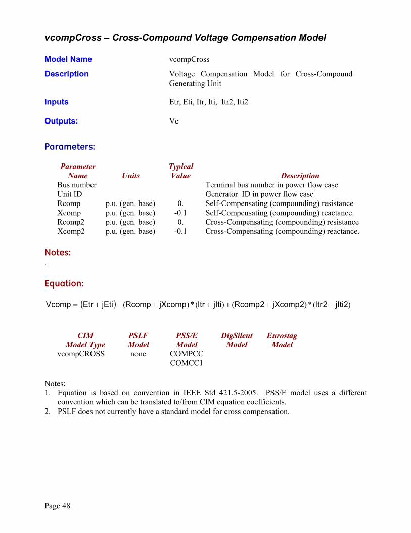
vcompCross – Cross-Compound Voltage Compensation Model Model Name vcompCross
Description Voltage Compensation Model for Cross-Compound Generating Unit
Inputs Etr, Eti, Itr, Iti, Itr2, Iti2 Outputs: Vc
Parameters:
Parameter Typical Name Units Value Description Bus number Terminal bus number in power flow case Unit ID Generator ID in power flow case Rcomp p.u. (gen. base) 0. Self-Compensating (compounding) resistance Xcomp p.u. (gen. base) -0.1 Self-Compensating (compounding) reactance. Rcomp2 p.u. (gen. base) 0. Cross-Compensating (compounding) resistance Xcomp2 p.u. (gen. base) -0.1 Cross-Compensating (compounding) reactance. Notes: . Equation:
( ) )(*)()(*)( 2jIti2Itr2jXcomp2RcompjItiItrjXcompRcompjEtiEtrVcomp +++++++= CIM PSLF PSS/E DigSilent Eurostag Model Type Model Model Model Model vcompCROSS none COMPCC
COMCC1
Notes: 1. Equation is based on convention in IEEE Std 421.5-2005. PSS/E model uses a different
convention which can be translated to/from CIM equation coefficients. 2. PSLF does not currently have a standard model for cross compensation.
Page 49
Excitation System Models The excitation system model provides the field voltage (Efd) for a synchronous machine model. It is linked to a specific generator by the Bus number and Unit ID. The data parameters are different for each excitation system model; the same parameter name may have different meaning in different models.
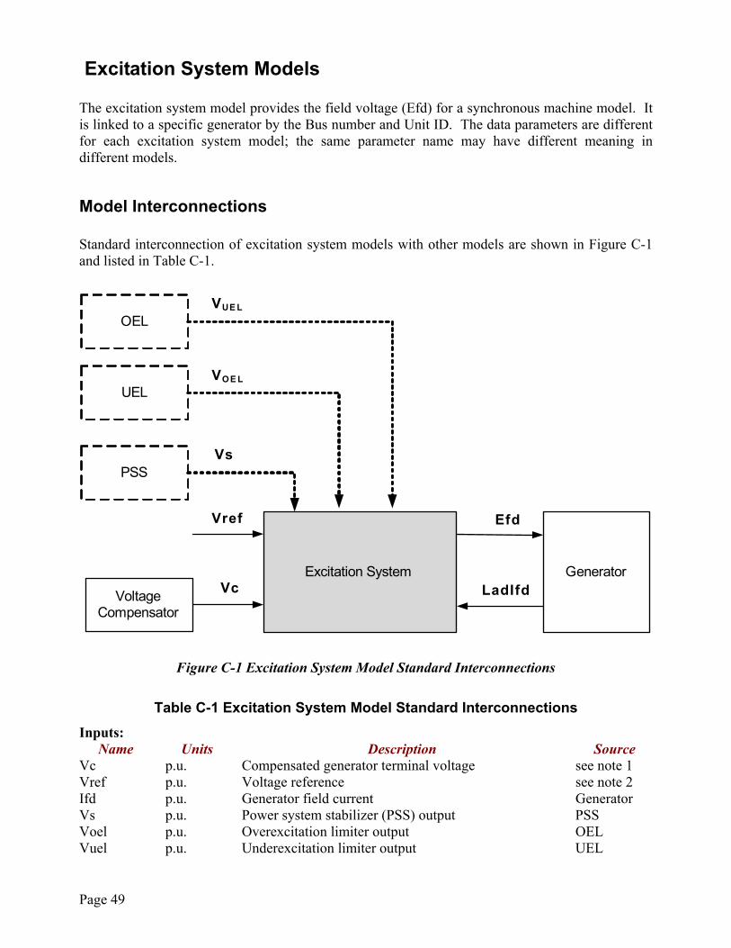
Model Interconnections Standard interconnection of excitation system models with other models are shown in Figure C-1 and listed in Table C-1.
Efd
LadIfd
Vref
Vs
VOE L
VUE L
Excitation SystemVc
Generator
VoltageCompensator
PSS
UEL
OEL
Figure C-1 Excitation System Model Standard Interconnections
Table C-1 Excitation System Model Standard Interconnections Inputs:
Name Units Description Source Vc p.u. Compensated generator terminal voltage see note 1 Vref p.u. Voltage reference see note 2 Ifd p.u. Generator field current Generator Vs p.u. Power system stabilizer (PSS) output PSS Voel p.u. Overexcitation limiter output OEL Vuel p.u. Underexcitation limiter output UEL
Page 50
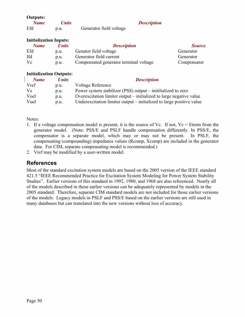
Outputs: Name Units Description
Efd p.u. Generator field voltage Initialization Inputs:
Name Units Description Source Efd p.u. Genator field voltage Generator Ifd p.u. Generator field current Generator Vc p.u. Compensated generator terminal voltage Compensator Initialization Outputs:
Name Units Description Vref p.u. Voltage Reference Vs p.u. Power system stabilizer (PSS) output – initilialized to zero Voel p.u. Overexcitation limiter output – initialized to large negative value Vuel p.u. Underexcitation limiter output – initialized to large positive value Notes: 1. If a voltage compensation model is present, it is the source of Vc. If not, Vc = Eterm from the
generator model. (Note: PSS/E and PSLF handle compensation differently. In PSS/E, the compensator is a separate model, which may or may not be present. In PSLF, the compensating (compounding) impedance values (Rcomp, Xcomp) are included in the generator data. For CIM, separate compensating model is recommended.)
2. Vref may be modified by a user-written model.
References Most of the standard excitation system models are based on the 2005 version of the IEEE standard 421.5 “IEEE Recommended Practice for Excitation System Modeling for Power System Stability Studies”. Earlier versions of this standard in 1992, 1980, and 1968 are also referenced. Nearly all of the models described in these earlier versions can be adequately represented by models in the 2005 standard. Therefore, separate CIM standard models are not included for those earlier versions of the models. Legacy models in PSLF and PSS/E based on the earlier versions are still used in many databases but can translated into the new versions without loss of accuracy.
Page 51
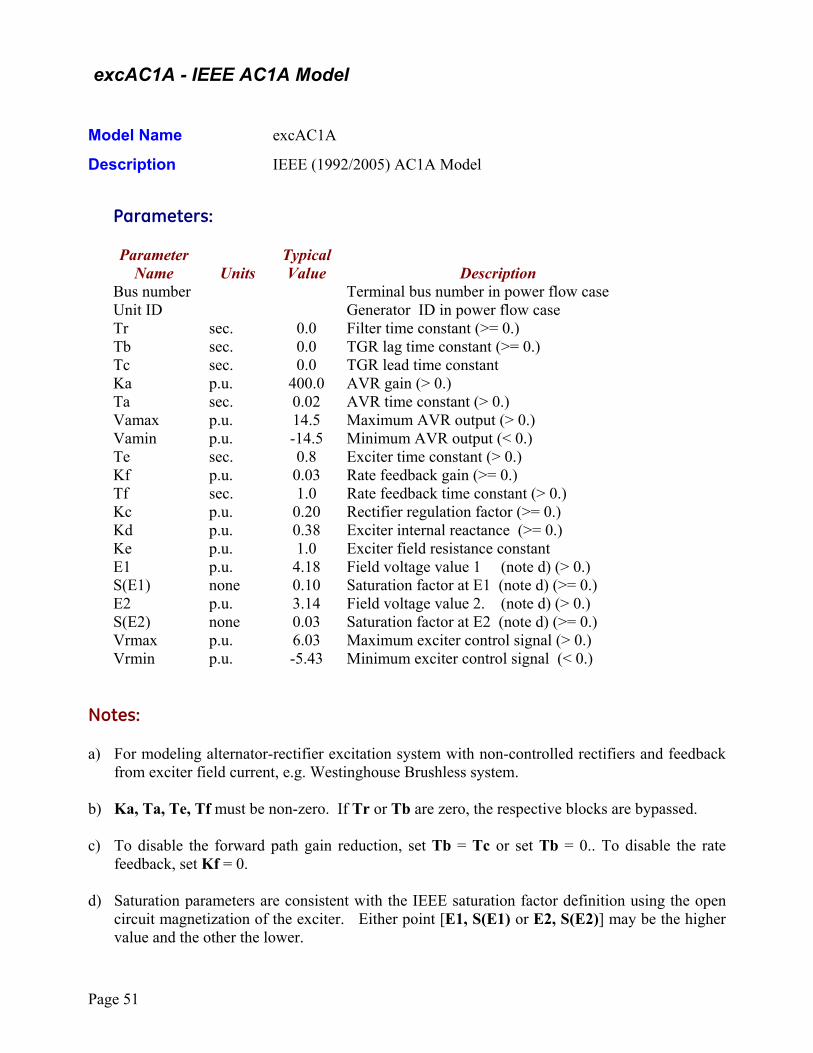
excAC1A - IEEE AC1A Model Model Name excAC1A
Description IEEE (1992/2005) AC1A Model
Parameters:
Parameter Typical Name Units Value Description Bus number Terminal bus number in power flow case Unit ID Generator ID in power flow case Tr sec. 0.0 Filter time constant (>= 0.) Tb sec. 0.0 TGR lag time constant (>= 0.) Tc sec. 0.0 TGR lead time constant Ka p.u. 400.0 AVR gain (> 0.) Ta sec. 0.02 AVR time constant (> 0.) Vamax p.u. 14.5 Maximum AVR output (> 0.) Vamin p.u. -14.5 Minimum AVR output (< 0.) Te sec. 0.8 Exciter time constant (> 0.) Kf p.u. 0.03 Rate feedback gain (>= 0.) Tf sec. 1.0 Rate feedback time constant (> 0.) Kc p.u. 0.20 Rectifier regulation factor (>= 0.) Kd p.u. 0.38 Exciter internal reactance (>= 0.) Ke p.u. 1.0 Exciter field resistance constant E1 p.u. 4.18 Field voltage value 1 (note d) (> 0.) S(E1) none 0.10 Saturation factor at E1 (note d) (>= 0.) E2 p.u. 3.14 Field voltage value 2. (note d) (> 0.) S(E2) none 0.03 Saturation factor at E2 (note d) (>= 0.) Vrmax p.u. 6.03 Maximum exciter control signal (> 0.) Vrmin p.u. -5.43 Minimum exciter control signal (< 0.) Notes: a) For modeling alternator-rectifier excitation system with non-controlled rectifiers and feedback
from exciter field current, e.g. Westinghouse Brushless system. b) Ka, Ta, Te, Tf must be non-zero. If Tr or Tb are zero, the respective blocks are bypassed. c) To disable the forward path gain reduction, set Tb = Tc or set Tb = 0.. To disable the rate
feedback, set Kf = 0. d) Saturation parameters are consistent with the IEEE saturation factor definition using the open
circuit magnetization of the exciter. Either point [E1, S(E1) or E2, S(E2)] may be the higher value and the other the lower.
Page 52
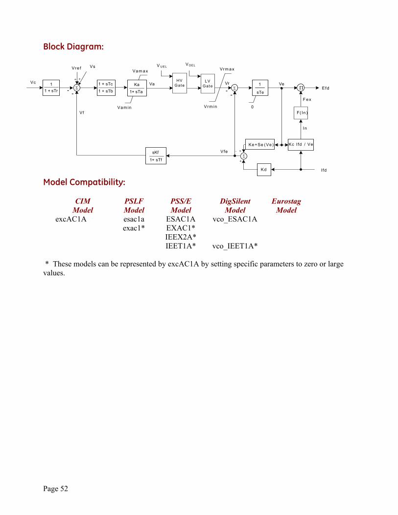
Block Diagram:
Kd
F( In )
F ex
Efd
Ke+Se (Ve ) Vfe
I fd
Vc+
+
+
-
0Vf
Vre f
In
Vrm a x
Vam in
Kc I fd / Ve
+
Vrm in
Vam ax
1 + sTb
1 + sTc1 + sTr
1 1
sTe
sKf
1+ sTf
1+ sTa
KaLV
GateVa Ve
Vs
Π
+
- Σ-
Σ
Σ
VOEL
VrHV
Gate
V U EL
Model Compatibility:
CIM PSLF PSS/E DigSilent Eurostag Model Model Model Model Model excAC1A esac1a ESAC1A vco_ESAC1A exac1* EXAC1* IEEX2A* IEET1A* vco_IEET1A* * These models can be represented by excAC1A by setting specific parameters to zero or large values.
Page 53
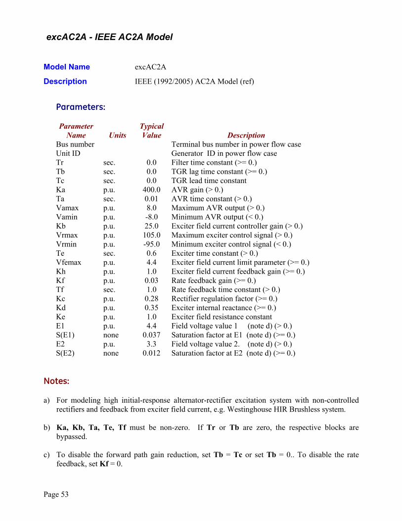
excAC2A - IEEE AC2A Model Model Name excAC2A
Description IEEE (1992/2005) AC2A Model (ref)
Parameters:
Parameter Typical Name Units Value Description Bus number Terminal bus number in power flow case Unit ID Generator ID in power flow case Tr sec. 0.0 Filter time constant (>= 0.) Tb sec. 0.0 TGR lag time constant (>= 0.) Tc sec. 0.0 TGR lead time constant Ka p.u. 400.0 AVR gain (> 0.) Ta sec. 0.01 AVR time constant (> 0.) Vamax p.u. 8.0 Maximum AVR output (> 0.) Vamin p.u. -8.0 Minimum AVR output (< 0.) Kb p.u. 25.0 Exciter field current controller gain (> 0.) Vrmax p.u. 105.0 Maximum exciter control signal (> 0.) Vrmin p.u. -95.0 Minimum exciter control signal (< 0.) Te sec. 0.6 Exciter time constant (> 0.) Vfemax p.u. 4.4 Exciter field current limit parameter (>= 0.) Kh p.u. 1.0 Exciter field current feedback gain (>= 0.) Kf p.u. 0.03 Rate feedback gain (>= 0.) Tf sec. 1.0 Rate feedback time constant (> 0.) Kc p.u. 0.28 Rectifier regulation factor (>= 0.) Kd p.u. 0.35 Exciter internal reactance (>= 0.) Ke p.u. 1.0 Exciter field resistance constant E1 p.u. 4.4 Field voltage value 1 (note d) (> 0.) S(E1) none 0.037 Saturation factor at E1 (note d) (>= 0.) E2 p.u. 3.3 Field voltage value 2. (note d) (> 0.) S(E2) none 0.012 Saturation factor at E2 (note d) (>= 0.) Notes: a) For modeling high initial-response alternator-rectifier excitation system with non-controlled
rectifiers and feedback from exciter field current, e.g. Westinghouse HIR Brushless system. b) Ka, Kb, Ta, Te, Tf must be non-zero. If Tr or Tb are zero, the respective blocks are
bypassed. c) To disable the forward path gain reduction, set Tb = Tc or set Tb = 0.. To disable the rate
feedback, set Kf = 0.
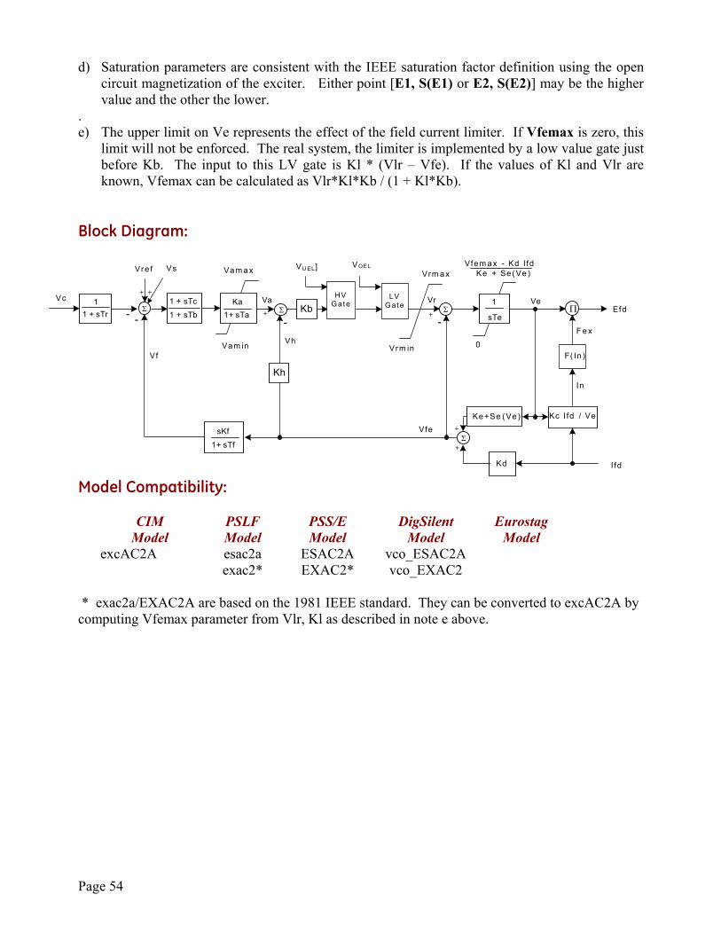
Page 54
d) Saturation parameters are consistent with the IEEE saturation factor definition using the open
circuit magnetization of the exciter. Either point [E1, S(E1) or E2, S(E2)] may be the higher value and the other the lower.
. e) The upper limit on Ve represents the effect of the field current limiter. If Vfemax is zero, this
limit will not be enforced. The real system, the limiter is implemented by a low value gate just before Kb. The input to this LV gate is Kl * (Vlr – Vfe). If the values of Kl and Vlr are known, Vfemax can be calculated as Vlr*Kl*Kb / (1 + Kl*Kb).
Block Diagram:
Kd
F( In )
F e x
Efd
Ke +Se (Ve) Vfe
I fd
+
+
+
-
0Vf
Vre f
In
Vrm ax
Vam in
Kc I fd / Ve
+
Vrm in
Va m a x
1 + sTb
1 + sTc1 + sTr
1 1
sTe
sKf
1+ sTf
1+ sTa Ka
LVG at e
Vc Va Ve
Vs
Π
+
- Σ-
Σ
Σ
Vfem a x - Kd I fdKe + Se (Ve )
VOEL
VrHVGate
Σ
Kh
Kb-
+
Vh
VU EL]
Model Compatibility:
CIM PSLF PSS/E DigSilent Eurostag Model Model Model Model Model excAC2A esac2a ESAC2A vco_ESAC2A exac2* EXAC2* vco_EXAC2 * exac2a/EXAC2A are based on the 1981 IEEE standard. They can be converted to excAC2A by computing Vfemax parameter from Vlr, Kl as described in note e above.
Page 55
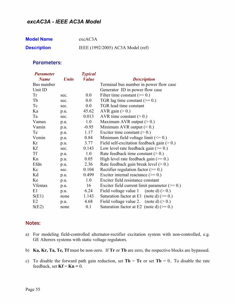
excAC3A - IEEE AC3A Model Model Name excAC3A
Description IEEE (1992/2005) AC3A Model (ref)
Parameters:
Parameter Typical Name Units Value Description Bus number Terminal bus number in power flow case Unit ID Generator ID in power flow case Tr sec. 0.0 Filter time constant (>= 0.) Tb sec. 0.0 TGR lag time constant (>= 0.) Tc sec. 0.0 TGR lead time constant Ka p.u. 45.62 AVR gain (> 0.) Ta sec. 0.013 AVR time constant (> 0.) Vamax p.u. 1.0 Maximum AVR output (> 0.) Vamin p.u. -0.95 Minimum AVR output (< 0.) Te p.u. 1.17 Exciter time constant (> 0.) Vemin p.u. 0.84 Minimum field voltage limit (<= 0.) Kr p.u. 3.77 Field self-excitation feedback gain (> 0.) Kf sec. 0.143 Low level rate feedback gain (>= 0.) Tf p.u. 1.0 Rate feedback time constant (> 0.) Kn p.u. 0.05 High level rate feedback gain (>= 0.) Efdn p.u. 2.36 Rate feedback gain break level (> 0.) Kc sec. 0.104 Rectifier regulation factor (>= 0.) Kd p.u. 0.499 Exciter internal reactance (>= 0.) Ke p.u. 1.0 Exciter field resistance constant Vfemax p.u. 16 Exciter field current limit parameter (>= 0.) E1 p.u. 6.24 Field voltage value 1 (note d) (> 0.) S(E1) none 1.143 Saturation factor at E1 (note d) (>= 0.) E2 p.u. 4.68 Field voltage value 2. (note d) (> 0.) S(E2) none 0.1 Saturation factor at E2 (note d) (>= 0.) Notes: a) For modeling field-controlled alternator-rectifier excitation system with non-controlled, e.g.
GE Alterrex systems with static voltage regulators. b) Ka, Kr, Ta, Te, Tf must be non-zero. If Tr or Tb are zero, the respective blocks are bypassed. c) To disable the forward path gain reduction, set Tb = Tc or set Tb = 0.. To disable the rate
feedback, set Kf = Kn = 0.
Page 56
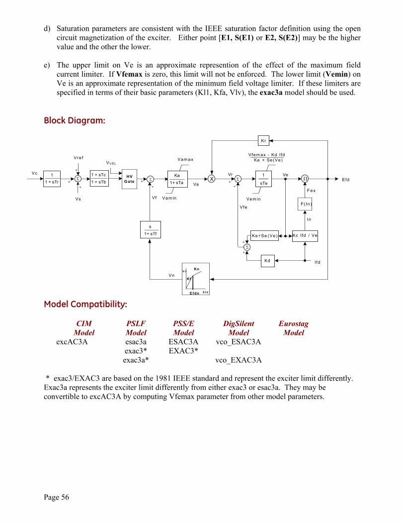
d) Saturation parameters are consistent with the IEEE saturation factor definition using the open circuit magnetization of the exciter. Either point [E1, S(E1) or E2, S(E2)] may be the higher value and the other the lower.
e) The upper limit on Ve is an approximate represention of the effect of the maximum field
current limiter. If Vfemax is zero, this limit will not be enforced. The lower limit (Vemin) on Ve is an approximate representation of the minimum field voltage limiter. If these limiters are specified in terms of their basic parameters (Kl1, Kfa, Vlv), the exac3a model should be used.
Block Diagram:
Kd
F( In )
F ex
Efd
Ke+Se (Ve)
Vfe
I fd
Vc+
+
+
-
VfVs
In
Va m in
Kc I fd / Ve
+
Vam ax
1 + sTb
1 + sTc
1 + sTr1 1
sTe
s
1+ sTf
1+ sTa
Ka
Va
Ve
Vre f
Π+
- Σ Σ
Σ
Vfem ax - Kd I fdKe + Se (Ve)
VrHVG ate Σ
-+
VU EL
X
Kr
Vem in
VnKn
Kf
E fdn
V n
E f d
Model Compatibility:
CIM PSLF PSS/E DigSilent Eurostag Model Model Model Model Model excAC3A esac3a ESAC3A vco_ESAC3A exac3* EXAC3* exac3a* vco_EXAC3A * exac3/EXAC3 are based on the 1981 IEEE standard and represent the exciter limit differently. Exac3a represents the exciter limit differently from either exac3 or esac3a. They may be convertible to excAC3A by computing Vfemax parameter from other model parameters.
Page 57
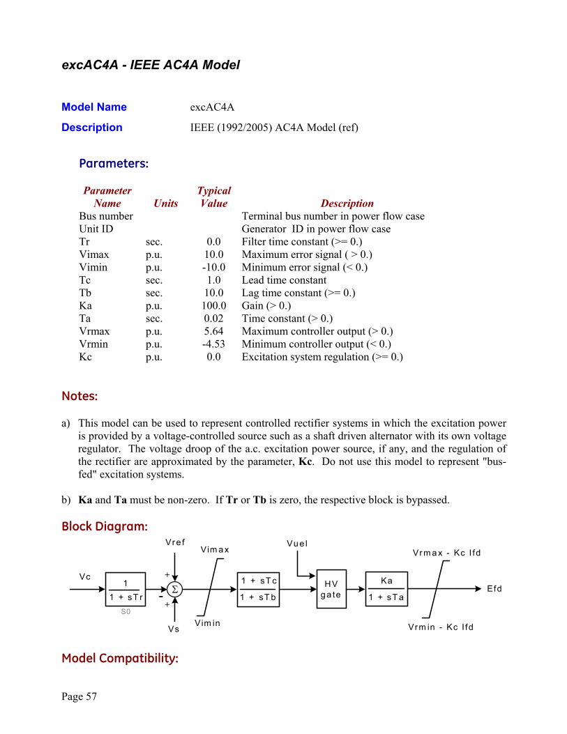
excAC4A - IEEE AC4A Model Model Name excAC4A
Description IEEE (1992/2005) AC4A Model (ref)
Parameters:
Parameter Typical Name Units Value Description Bus number Terminal bus number in power flow case Unit ID Generator ID in power flow case Tr sec. 0.0 Filter time constant (>= 0.) Vimax p.u. 10.0 Maximum error signal ( > 0.) Vimin p.u. -10.0 Minimum error signal (< 0.) Tc sec. 1.0 Lead time constant Tb sec. 10.0 Lag time constant (>= 0.) Ka p.u. 100.0 Gain (> 0.) Ta sec. 0.02 Time constant (> 0.) Vrmax p.u. 5.64 Maximum controller output (> 0.) Vrmin p.u. -4.53 Minimum controller output (< 0.) Kc p.u. 0.0 Excitation system regulation (>= 0.) Notes: a) This model can be used to represent controlled rectifier systems in which the excitation power
is provided by a voltage-controlled source such as a shaft driven alternator with its own voltage regulator. The voltage droop of the a.c. excitation power source, if any, and the regulation of the rectifier are approximated by the parameter, Kc. Do not use this model to represent "bus-fed" excitation systems.
b) Ka and Ta must be non-zero. If Tr or Tb is zero, the respective block is bypassed.
Block Diagram:
Efd
S0
+
+
Vre f
1 + sT r1
-
Vim a x
Vim in
1 + sT a
Ka
1 + sT b
1 + sT c
Vrm a x - Kc I fd
Vrm in - Kc I fd
ΣVc
Vs
HVga te
Vue l
Model Compatibility:
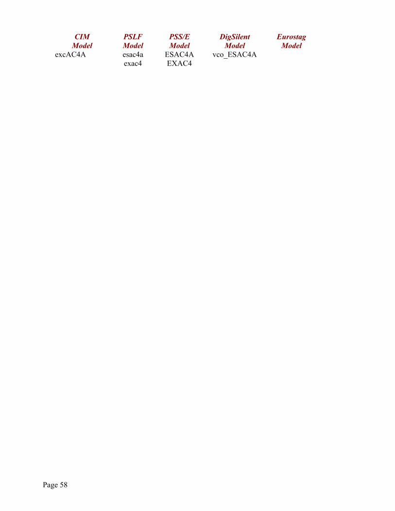
Page 58
CIM PSLF PSS/E DigSilent Eurostag Model Model Model Model Model excAC4A esac4a ESAC4A vco_ESAC4A exac4 EXAC4
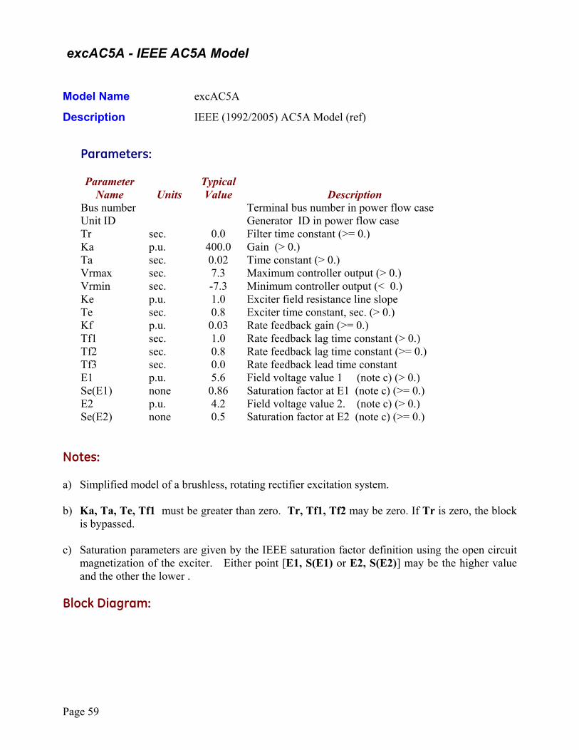
Page 59
excAC5A - IEEE AC5A Model Model Name excAC5A
Description IEEE (1992/2005) AC5A Model (ref)
Parameters:
Parameter Typical Name Units Value Description Bus number Terminal bus number in power flow case Unit ID Generator ID in power flow case Tr sec. 0.0 Filter time constant (>= 0.) Ka p.u. 400.0 Gain (> 0.) Ta sec. 0.02 Time constant (> 0.) Vrmax sec. 7.3 Maximum controller output (> 0.) Vrmin sec. -7.3 Minimum controller output (< 0.) Ke p.u. 1.0 Exciter field resistance line slope Te sec. 0.8 Exciter time constant, sec. (> 0.) Kf p.u. 0.03 Rate feedback gain (>= 0.) Tf1 sec. 1.0 Rate feedback lag time constant (> 0.) Tf2 sec. 0.8 Rate feedback lag time constant (>= 0.) Tf3 sec. 0.0 Rate feedback lead time constant E1 p.u. 5.6 Field voltage value 1 (note c) (> 0.) Se(E1) none 0.86 Saturation factor at E1 (note c) (>= 0.) E2 p.u. 4.2 Field voltage value 2. (note c) (> 0.) Se(E2) none 0.5 Saturation factor at E2 (note c) (>= 0.) Notes: a) Simplified model of a brushless, rotating rectifier excitation system.
b) Ka, Ta, Te, Tf1 must be greater than zero. Tr, Tf1, Tf2 may be zero. If Tr is zero, the block
is bypassed.
c) Saturation parameters are given by the IEEE saturation factor definition using the open circuit magnetization of the exciter. Either point [E1, S(E1) or E2, S(E2)] may be the higher value and the other the lower .
Block Diagram:
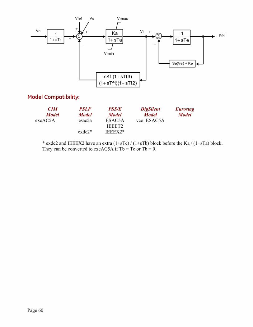
Page 60
ΣΣ Efd
Se(Ve) + Ke
Vrmin
Vrmax
Vc
sTr11
+ sTa1Ka
+
)2sTf1()1sTf1()3sTf1(sKf
+++
sTe11
+
Vref Vs
++ +
−
−
−
Vr
Model Compatibility:
CIM PSLF PSS/E DigSilent Eurostag Model Model Model Model Model excAC5A esac5a ESAC5A vco_ESAC5A IEEET2 exdc2* IEEEX2*
* exdc2 and IEEEX2 have an extra (1+sTc) / (1+sTb) block before the Ka / (1+sTa) block. They can be converted to excAC5A if Tb = Tc or Tb = 0.
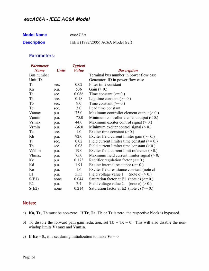
Page 61
excAC6A - IEEE AC6A Model Model Name excAC6A
Description IEEE (1992/2005) AC6A Model (ref)
Parameters:
Parameter Typical Name Units Value Description Bus number Terminal bus number in power flow case Unit ID Generator ID in power flow case Tr sec. 0.02 Filter time constant Ka p.u. 536 Gain (> 0.) Ta sec. 0.086 Time constant (>= 0.) Tk sec. 0.18 Lag time constant (>= 0.) Tb sec. 9.0 Time constant (>= 0.) Tc sec. 3.0 Lead time constant Vamax p.u. 75.0 Maximum controller element output (> 0.) Vamin p.u. -75.0 Minimum controller element output (< 0.) Vrmax p.u. 44.0 Maximum exciter control signal (> 0.) Vrmin p.u. -36.0 Minimum exciter control signal (< 0.) Te sec. 1.0 Exciter time constant (> 0.) Kh p.u. 92.0 Exciter field current limiter gain (>= 0.) Tj sec. 0.02 Field current limiter time constant (>= 0.) Th sec. 0.08 Field current limiter time constant (> 0.) Vfelim p.u. 19.0 Exciter field current limit reference (> 0.) Vhmax p.u. 75.0 Maximum field current limiter signal (> 0.) Kc p.u. 0.173 Rectifier regulation factor (>= 0.) Kd p.u. 1.91 Exciter internal reactance (>= 0.) Ke p.u. 1.6 Exciter field resistance constant (note c) E1 p.u. 5.55 Field voltage value 1 (note c) (> 0.) S(E1) none 0.044 Saturation factor at E1 (note c) (>= 0.) E2 p.u. 7.4 Field voltage value 2. (note c) (> 0.) S(E2) none 0.214 Saturation factor at E2 (note c) (>= 0.) Notes: a) Ka, Te, Th must be non-zero. If Tr, Ta, Tb or Tc is zero, the respective block is bypassed. b) To disable the forward path gain reduction, set Tb = Tc = 0. This will also disable the non-
windup limits Vamax and Vamin. c) If Ke = 0., it is set during initialization to make Vr = 0.
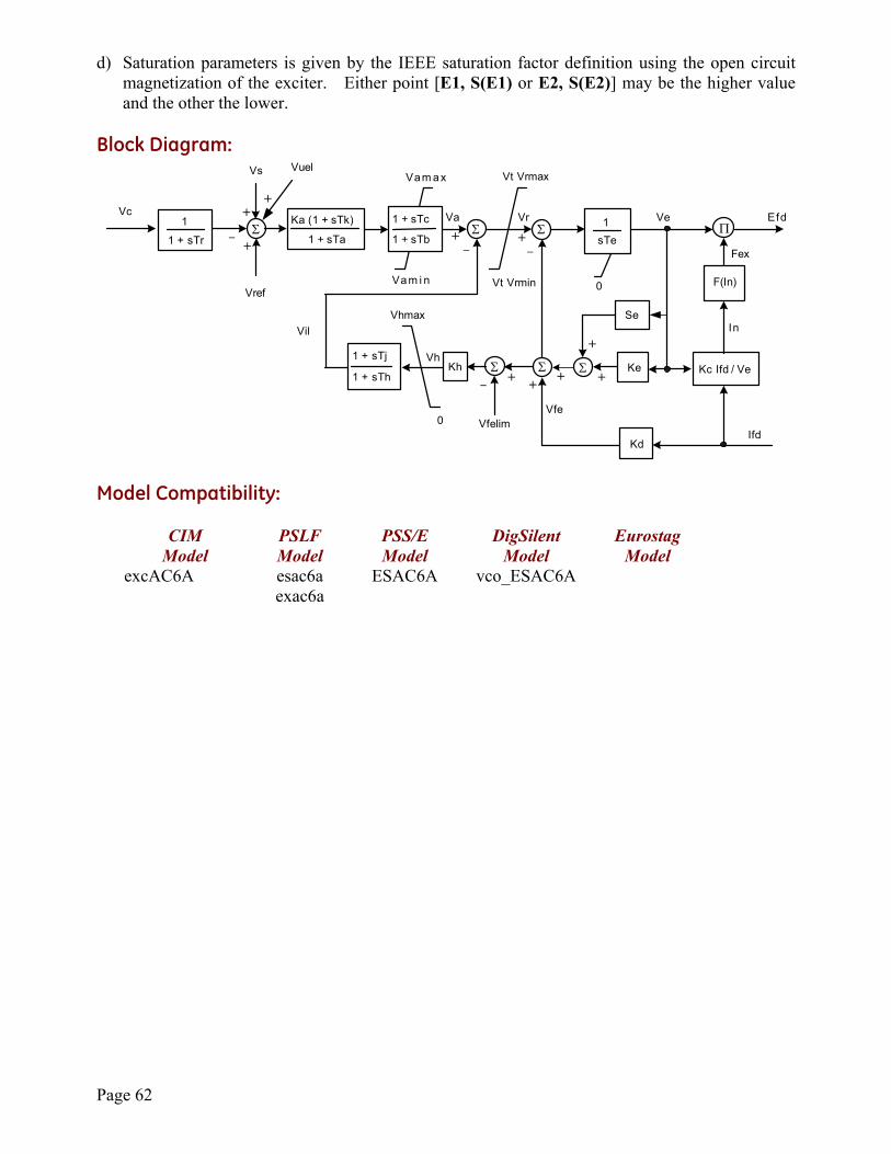
Page 62
d) Saturation parameters is given by the IEEE saturation factor definition using the open circuit magnetization of the exciter. Either point [E1, S(E1) or E2, S(E2)] may be the higher value and the other the lower.
Block Diagram:
Kd
F(In)
Fex
Efd
Ifd
+ +
In
Ve
+
Se
Ke
1sTe
0
+
+
Vc +
+−
Vs Vt Vrmax
Va m i n Vt Vrmin
Vam a x
Vref
1 + sTa
Ka (1 + sTk)
1 + sTb
1 + sTc Va
+Vr
Vhmax
1 + sTh
1 + sTj VhKh
+
Vfelim0
Kc Ifd / Ve
1
1 + sTrΠ
Vfe
Vil
Σ
Σ Σ Σ
Σ Σ
− −
−
Vuel
+
Model Compatibility:
CIM PSLF PSS/E DigSilent Eurostag Model Model Model Model Model excAC6A esac6a ESAC6A vco_ESAC6A exac6a
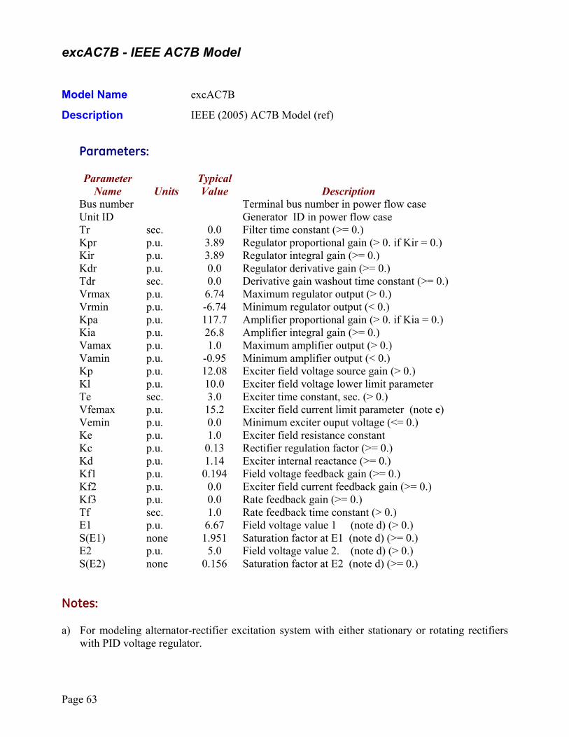
Page 63
excAC7B - IEEE AC7B Model Model Name excAC7B
Description IEEE (2005) AC7B Model (ref)
Parameters:
Parameter Typical Name Units Value Description Bus number Terminal bus number in power flow case Unit ID Generator ID in power flow case Tr sec. 0.0 Filter time constant (>= 0.) Kpr p.u. 3.89 Regulator proportional gain (> 0. if Kir = 0.) Kir p.u. 3.89 Regulator integral gain (>= 0.) Kdr p.u. 0.0 Regulator derivative gain (>= 0.) Tdr sec. 0.0 Derivative gain washout time constant (>= 0.) Vrmax p.u. 6.74 Maximum regulator output (> 0.) Vrmin p.u. -6.74 Minimum regulator output (< 0.) Kpa p.u. 117.7 Amplifier proportional gain (> 0. if Kia = 0.) Kia p.u. 26.8 Amplifier integral gain (>= 0.) Vamax p.u. 1.0 Maximum amplifier output (> 0.) Vamin p.u. -0.95 Minimum amplifier output (< 0.) Kp p.u. 12.08 Exciter field voltage source gain (> 0.) Kl p.u. 10.0 Exciter field voltage lower limit parameter Te sec. 3.0 Exciter time constant, sec. (> 0.) Vfemax p.u. 15.2 Exciter field current limit parameter (note e) Vemin p.u. 0.0 Minimum exciter ouput voltage (<= 0.) Ke p.u. 1.0 Exciter field resistance constant Kc p.u. 0.13 Rectifier regulation factor (>= 0.) Kd p.u. 1.14 Exciter internal reactance (>= 0.) Kf1 p.u. 0.194 Field voltage feedback gain (>= 0.) Kf2 p.u. 0.0 Exciter field current feedback gain (>= 0.) Kf3 p.u. 0.0 Rate feedback gain (>= 0.) Tf sec. 1.0 Rate feedback time constant (> 0.) E1 p.u. 6.67 Field voltage value 1 (note d) (> 0.) S(E1) none 1.951 Saturation factor at E1 (note d) (>= 0.) E2 p.u. 5.0 Field voltage value 2. (note d) (> 0.) S(E2) none 0.156 Saturation factor at E2 (note d) (>= 0.) Notes: a) For modeling alternator-rectifier excitation system with either stationary or rotating rectifiers
with PID voltage regulator.
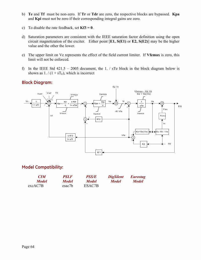
Page 64
b) Te and Tf must be non-zero. If Tr or Tdr are zero, the respective blocks are bypassed. Kpa and Kpi must not be zero if their corresponding integral gains are zero.
c) To disable the rate feedback, set Kf3 = 0. d) Saturation parameters are consistent with the IEEE saturation factor definition using the open
circuit magnetization of the exciter. Either point [E1, S(E1) or E2, S(E2)] may be the higher value and the other the lower.
e) The upper limit on Ve represents the effect of the field current limiter. If Vfemax is zero, this
limit will not be enforced. f) In the IEEE Std 421.5 – 2005 document, the 1. / sTe block in the block diagram below is
shown as 1. / (1 + sTE), which is incorrect
Block Diagram:
Kd
F( In )
F e xEfd
Ke+Se(Ve )
Vfe
I fd
+
+
+
-
Vf
Vre f
In
Va m in
Kc I fd / Ve
+
-Kl Vfe
Va m a x
1 + sTr
1 1
sTe
s Kf 3
1+ sTf
Vc Va Ve+
- Σ-
Σ
Σ
Vfem a x - Kd I fdKe + Se (Ve )
VrΣ
-
Vem in
Π
Kp Vt
Σ
Vu e l
+
Kpa + Kias
+
+Kf 2
Kf 1
Π
Vs
+
Vrm a x
Vrm in
1+ sTdr
s KdrKpr +
Kirs
+
Model Compatibility:
CIM PSLF PSS/E DigSilent Eurostag Model Model Model Model Model excAC7B esac7b ESAC7B
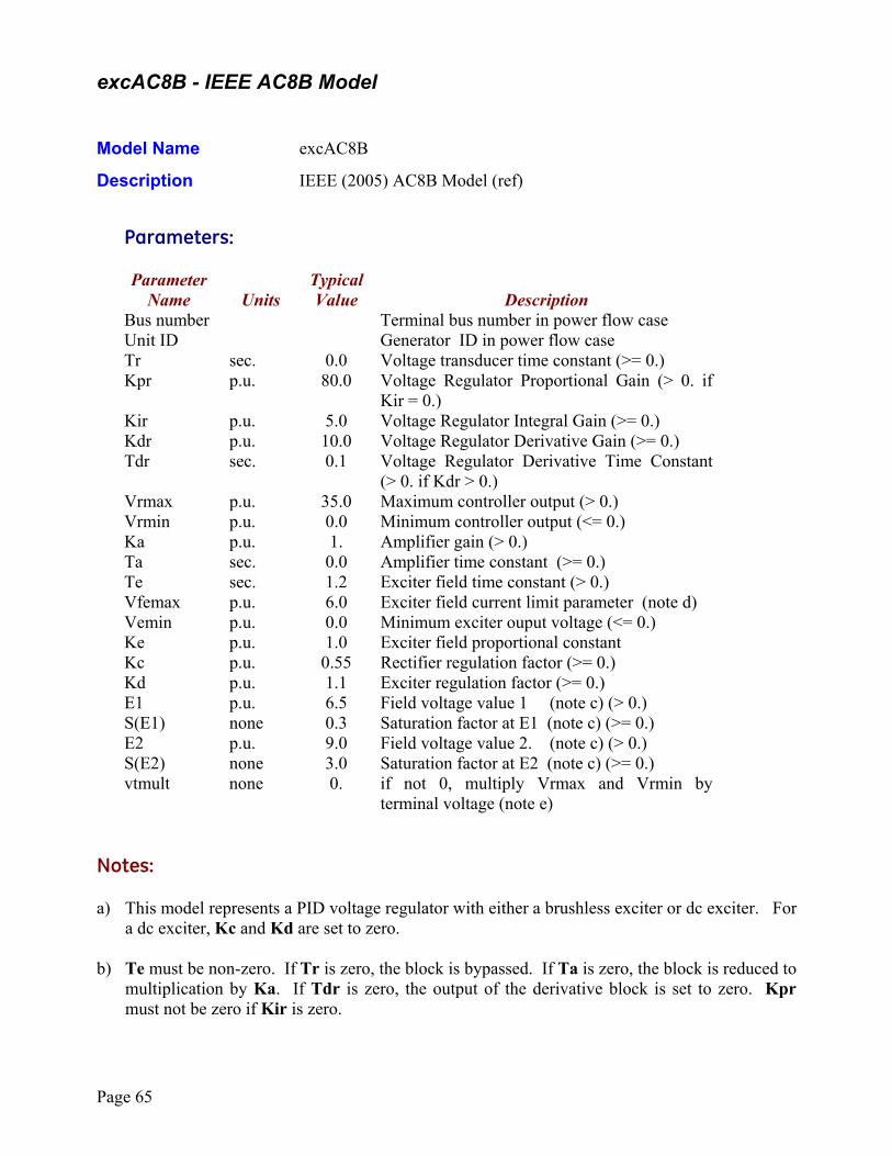
Page 65
excAC8B - IEEE AC8B Model Model Name excAC8B
Description IEEE (2005) AC8B Model (ref)
Parameters:
Parameter Typical Name Units Value Description Bus number Terminal bus number in power flow case Unit ID Generator ID in power flow case Tr sec. 0.0 Voltage transducer time constant (>= 0.) Kpr p.u. 80.0 Voltage Regulator Proportional Gain (> 0. if
Kir = 0.) Kir p.u. 5.0 Voltage Regulator Integral Gain (>= 0.) Kdr p.u. 10.0 Voltage Regulator Derivative Gain (>= 0.) Tdr sec. 0.1 Voltage Regulator Derivative Time Constant
(> 0. if Kdr > 0.) Vrmax p.u. 35.0 Maximum controller output (> 0.) Vrmin p.u. 0.0 Minimum controller output (<= 0.) Ka p.u. 1. Amplifier gain (> 0.) Ta sec. 0.0 Amplifier time constant (>= 0.) Te sec. 1.2 Exciter field time constant (> 0.) Vfemax p.u. 6.0 Exciter field current limit parameter (note d) Vemin p.u. 0.0 Minimum exciter ouput voltage (<= 0.) Ke p.u. 1.0 Exciter field proportional constant Kc p.u. 0.55 Rectifier regulation factor (>= 0.) Kd p.u. 1.1 Exciter regulation factor (>= 0.) E1 p.u. 6.5 Field voltage value 1 (note c) (> 0.) S(E1) none 0.3 Saturation factor at E1 (note c) (>= 0.) E2 p.u. 9.0 Field voltage value 2. (note c) (> 0.) S(E2) none 3.0 Saturation factor at E2 (note c) (>= 0.) vtmult none 0. if not 0, multiply Vrmax and Vrmin by
terminal voltage (note e) Notes: a) This model represents a PID voltage regulator with either a brushless exciter or dc exciter. For
a dc exciter, Kc and Kd are set to zero. b) Te must be non-zero. If Tr is zero, the block is bypassed. If Ta is zero, the block is reduced to
multiplication by Ka. If Tdr is zero, the output of the derivative block is set to zero. Kpr must not be zero if Kir is zero.
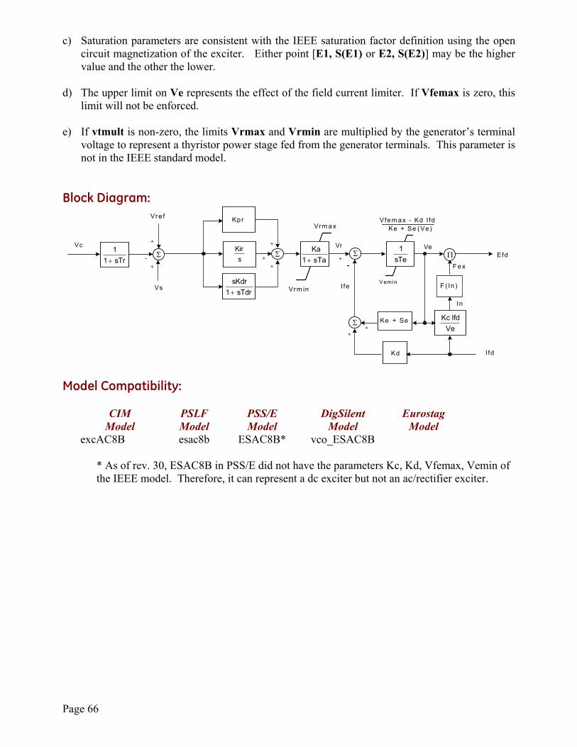
Page 66
c) Saturation parameters are consistent with the IEEE saturation factor definition using the open circuit magnetization of the exciter. Either point [E1, S(E1) or E2, S(E2)] may be the higher value and the other the lower.
d) The upper limit on Ve represents the effect of the field current limiter. If Vfemax is zero, this
limit will not be enforced. e) If vtmult is non-zero, the limits Vrmax and Vrmin are multiplied by the generator’s terminal
voltage to represent a thyristor power stage fed from the generator terminals. This parameter is not in the IEEE standard model.
Block Diagram:
Kd
F ( In )
F ex
Ke + Se
+
+
--
V emi n
+
+
Vrm in
++
+
I fe
In
sTdr1sKdr+
sTr11
+
VeIfdKc
sTe1
+sKir
Kp r
sTa1Ka
+
Vrm ax
Σ Σ Σ
Σ
Vc
Vre f
Vs
VrEfd
I fd
VeΠ
Vfem ax - Kd I fdKe + Se (Ve )
Model Compatibility:
CIM PSLF PSS/E DigSilent Eurostag Model Model Model Model Model excAC8B esac8b ESAC8B* vco_ESAC8B
* As of rev. 30, ESAC8B in PSS/E did not have the parameters Kc, Kd, Vfemax, Vemin of the IEEE model. Therefore, it can represent a dc exciter but not an ac/rectifier exciter.
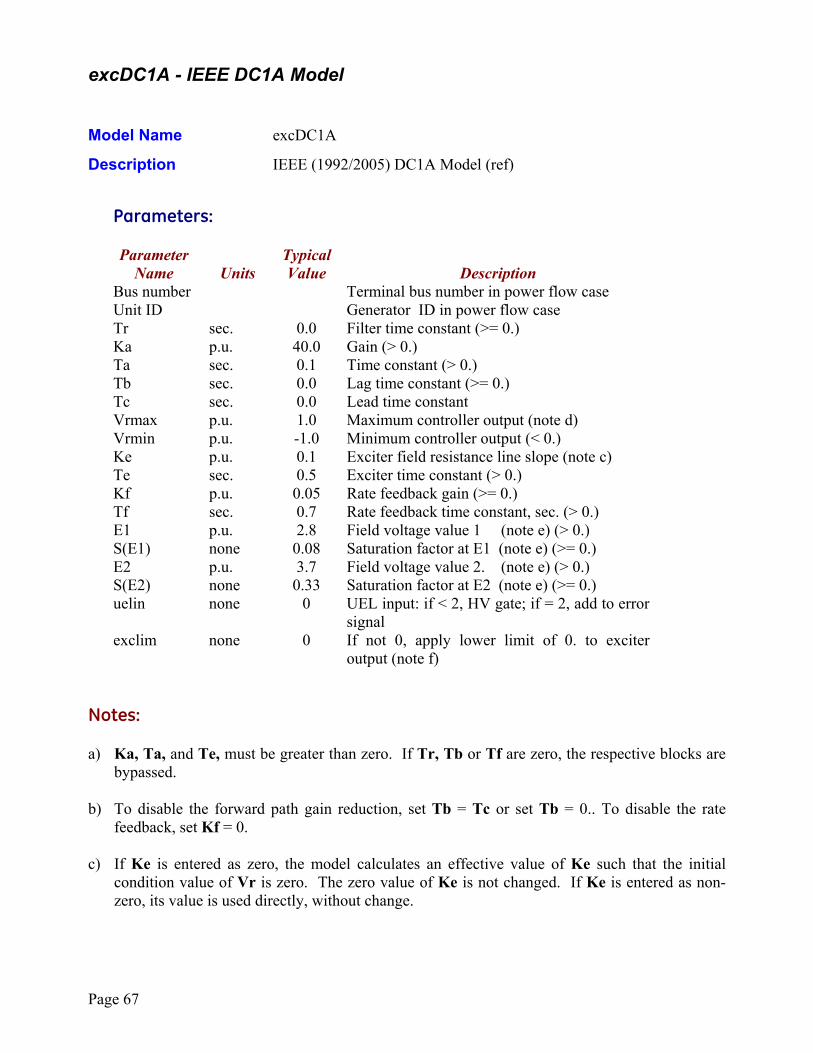
Page 67
excDC1A - IEEE DC1A Model Model Name excDC1A
Description IEEE (1992/2005) DC1A Model (ref)
Parameters:
Parameter Typical Name Units Value Description Bus number Terminal bus number in power flow case Unit ID Generator ID in power flow case Tr sec. 0.0 Filter time constant (>= 0.) Ka p.u. 40.0 Gain (> 0.) Ta sec. 0.1 Time constant (> 0.) Tb sec. 0.0 Lag time constant (>= 0.) Tc sec. 0.0 Lead time constant Vrmax p.u. 1.0 Maximum controller output (note d) Vrmin p.u. -1.0 Minimum controller output (< 0.) Ke p.u. 0.1 Exciter field resistance line slope (note c) Te sec. 0.5 Exciter time constant (> 0.) Kf p.u. 0.05 Rate feedback gain (>= 0.) Tf sec. 0.7 Rate feedback time constant, sec. (> 0.) E1 p.u. 2.8 Field voltage value 1 (note e) (> 0.) S(E1) none 0.08 Saturation factor at E1 (note e) (>= 0.) E2 p.u. 3.7 Field voltage value 2. (note e) (> 0.) S(E2) none 0.33 Saturation factor at E2 (note e) (>= 0.) uelin none 0 UEL input: if < 2, HV gate; if = 2, add to error
signal exclim none 0 If not 0, apply lower limit of 0. to exciter
output (note f) Notes: a) Ka, Ta, and Te, must be greater than zero. If Tr, Tb or Tf are zero, the respective blocks are
bypassed. b) To disable the forward path gain reduction, set Tb = Tc or set Tb = 0.. To disable the rate
feedback, set Kf = 0. c) If Ke is entered as zero, the model calculates an effective value of Ke such that the initial
condition value of Vr is zero. The zero value of Ke is not changed. If Ke is entered as non-zero, its value is used directly, without change.
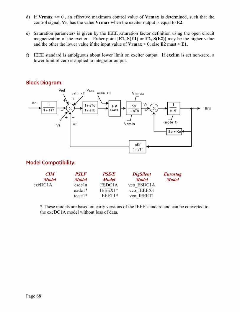
Page 68
d) If Vrmax <= 0., an effective maximum control value of Vrmax is determined, such that the control signal, Vr, has the value Vrmax when the exciter output is equal to E2.
e) Saturation parameters is given by the IEEE saturation factor definition using the open circuit
magnetization of the exciter. Either point [E1, S(E1) or E2, S(E2)] may be the higher value and the other the lower value if the input value of Vrmax > 0; else E2 must > E1.
f) IEEE standard is ambiguous about lower limit on exciter output. If exclim is set non-zero, a
lower limit of zero is applied to integrator output.
Block Diagram:
Efd
Se + Ke
+Vrm in
+
Vrm ax
Vr
sTb1sTc1
++
sTaKa
+1 sTe1
sTf1sKf+
Vs
−ΣHV
Gate
Vref
sTr11
+
+
Σ
−
−
VU EL
+uel i n < 2uel i n = 2
Vc
Vf (no te f )
Model Compatibility:
CIM PSLF PSS/E DigSilent Eurostag Model Model Model Model Model excDC1A esdc1a ESDC1A vco_ESDC1A exdc1* IEEEX1* vco_IEEEX1 ieeet1* IEEET1* vco_IEEET1
* These models are based on early versions of the IEEE standard and can be converted to the excDC1A model without loss of data.
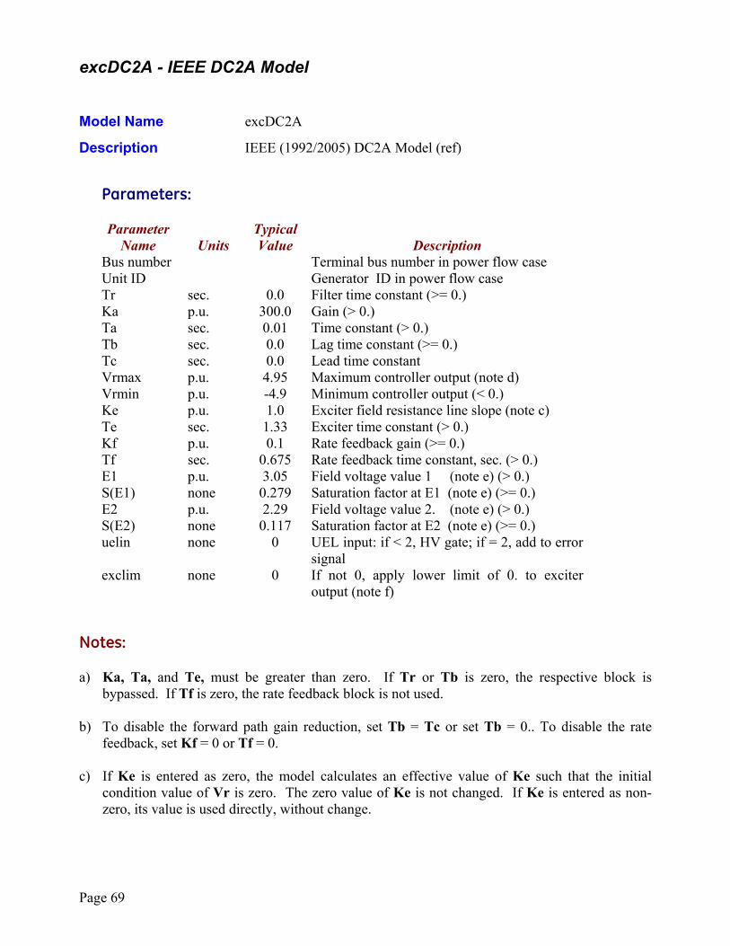
Page 69
excDC2A - IEEE DC2A Model Model Name excDC2A
Description IEEE (1992/2005) DC2A Model (ref)
Parameters:
Parameter Typical Name Units Value Description Bus number Terminal bus number in power flow case Unit ID Generator ID in power flow case Tr sec. 0.0 Filter time constant (>= 0.) Ka p.u. 300.0 Gain (> 0.) Ta sec. 0.01 Time constant (> 0.) Tb sec. 0.0 Lag time constant (>= 0.) Tc sec. 0.0 Lead time constant Vrmax p.u. 4.95 Maximum controller output (note d) Vrmin p.u. -4.9 Minimum controller output (< 0.) Ke p.u. 1.0 Exciter field resistance line slope (note c) Te sec. 1.33 Exciter time constant (> 0.) Kf p.u. 0.1 Rate feedback gain (>= 0.) Tf sec. 0.675 Rate feedback time constant, sec. (> 0.) E1 p.u. 3.05 Field voltage value 1 (note e) (> 0.) S(E1) none 0.279 Saturation factor at E1 (note e) (>= 0.) E2 p.u. 2.29 Field voltage value 2. (note e) (> 0.) S(E2) none 0.117 Saturation factor at E2 (note e) (>= 0.) uelin none 0 UEL input: if < 2, HV gate; if = 2, add to error
signal exclim none 0 If not 0, apply lower limit of 0. to exciter
output (note f) Notes: a) Ka, Ta, and Te, must be greater than zero. If Tr or Tb is zero, the respective block is
bypassed. If Tf is zero, the rate feedback block is not used. b) To disable the forward path gain reduction, set Tb = Tc or set Tb = 0.. To disable the rate
feedback, set Kf = 0 or Tf = 0. c) If Ke is entered as zero, the model calculates an effective value of Ke such that the initial
condition value of Vr is zero. The zero value of Ke is not changed. If Ke is entered as non-zero, its value is used directly, without change.
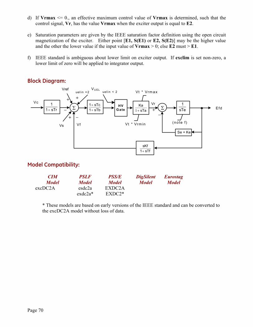
Page 70
d) If Vrmax <= 0., an effective maximum control value of Vrmax is determined, such that the control signal, Vr, has the value Vrmax when the exciter output is equal to E2.
e) Saturation parameters are given by the IEEE saturation factor definition using the open circuit
magnetization of the exciter. Either point [E1, S(E1) or E2, S(E2)] may be the higher value and the other the lower value if the input value of Vrmax > 0; else E2 must > E1.
f) IEEE standard is ambiguous about lower limit on exciter output. If exclim is set non-zero, a
lower limit of zero will be applied to integrator output.
Block Diagram:
Efd
Se + Ke
+Vt * Vrm in
+
Vt * Vrm ax
Vr
sTb1sTc1
++
sTaKa
+1 sTe1
sTf1sKf+
Vs
−ΣHV
Gate
Vref
sTr11
+
+
Σ
−
−
VU EL
+uel i n < 2uel i n = 2
Vc
Vf (no te f )
Model Compatibility:
CIM PSLF PSS/E DigSilent Eurostag Model Model Model Model Model excDC2A esdc2a EXDC2A exdc2a* EXDC2*
* These models are based on early versions of the IEEE standard and can be converted to the excDC2A model without loss of data.
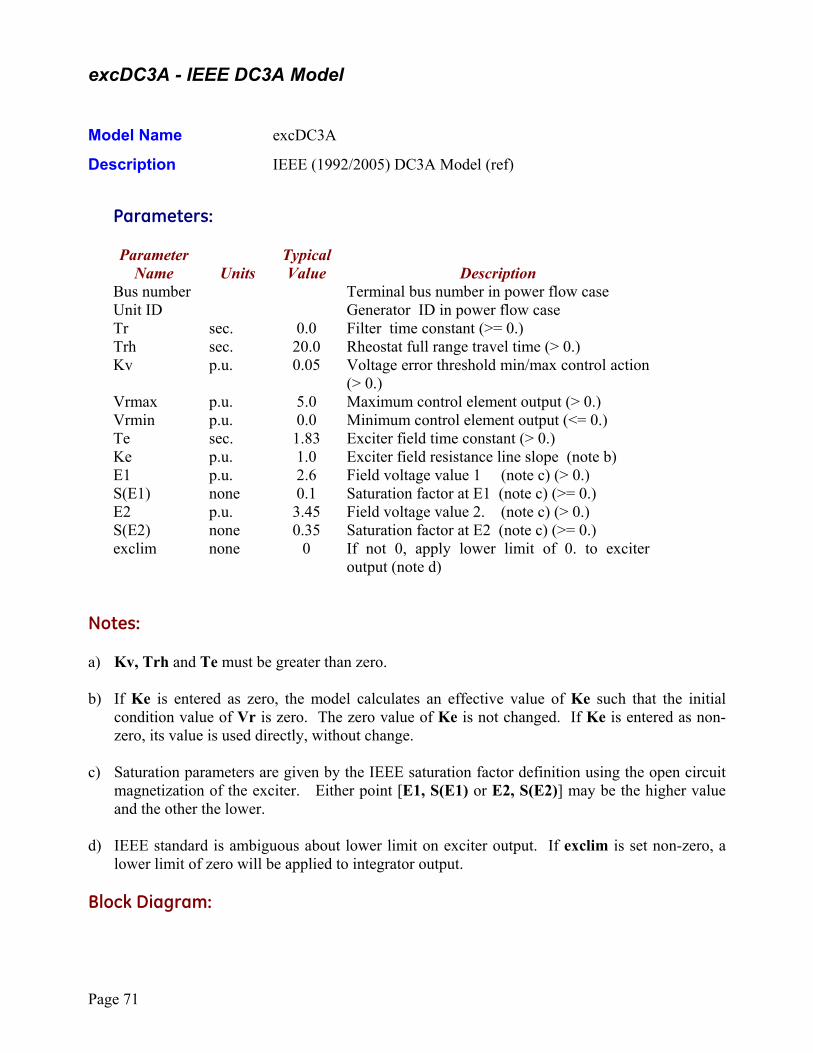
Page 71
excDC3A - IEEE DC3A Model Model Name excDC3A
Description IEEE (1992/2005) DC3A Model (ref)
Parameters:
Parameter Typical Name Units Value Description Bus number Terminal bus number in power flow case Unit ID Generator ID in power flow case Tr sec. 0.0 Filter time constant (>= 0.) Trh sec. 20.0 Rheostat full range travel time (> 0.) Kv p.u. 0.05 Voltage error threshold min/max control action
(> 0.) Vrmax p.u. 5.0 Maximum control element output (> 0.) Vrmin p.u. 0.0 Minimum control element output (<= 0.) Te sec. 1.83 Exciter field time constant (> 0.) Ke p.u. 1.0 Exciter field resistance line slope (note b) E1 p.u. 2.6 Field voltage value 1 (note c) (> 0.) S(E1) none 0.1 Saturation factor at E1 (note c) (>= 0.) E2 p.u. 3.45 Field voltage value 2. (note c) (> 0.) S(E2) none 0.35 Saturation factor at E2 (note c) (>= 0.) exclim none 0 If not 0, apply lower limit of 0. to exciter
output (note d) Notes: a) Kv, Trh and Te must be greater than zero. b) If Ke is entered as zero, the model calculates an effective value of Ke such that the initial
condition value of Vr is zero. The zero value of Ke is not changed. If Ke is entered as non-zero, its value is used directly, without change.
c) Saturation parameters are given by the IEEE saturation factor definition using the open circuit
magnetization of the exciter. Either point [E1, S(E1) or E2, S(E2)] may be the higher value and the other the lower.
d) IEEE standard is ambiguous about lower limit on exciter output. If exclim is set non-zero, a
lower limit of zero will be applied to integrator output.
Block Diagram:
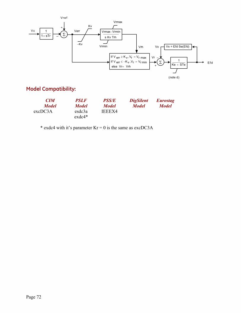
Page 72
Efd
Vre f
−
+
Vrmax
Vr
Vrh
Verr
STeKe1
+VrhVrelseminrVrV,vKerrVIf
maxrVrV,vKerrVIf
=
=−≤
=≥
Vx = Efd Se(Efd) Vx
Kv
−Kv
Vrmax−Vrmin
s Kv Trh
Vrmin
+
ΣsTr11
+ −Vc
(note d)
Σ
Model Compatibility:
CIM PSLF PSS/E DigSilent Eurostag Model Model Model Model Model excDC3A esdc3a IEEEX4 exdc4*
* exdc4 with it’s parameter Kr = 0 is the same as excDC3A
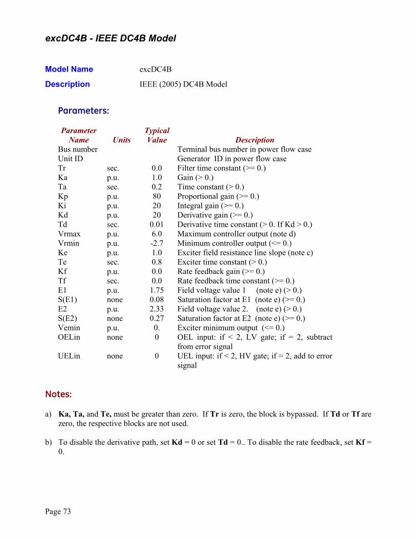
Page 73
excDC4B - IEEE DC4B Model Model Name excDC4B
Description IEEE (2005) DC4B Model
Parameters:
Parameter Typical Name Units Value Description Bus number Terminal bus number in power flow case Unit ID Generator ID in power flow case Tr sec. 0.0 Filter time constant (>= 0.) Ka p.u. 1.0 Gain (> 0.) Ta sec. 0.2 Time constant (> 0.) Kp p.u. 80 Proportional gain (>= 0.) Ki p.u. 20 Integral gain (>= 0.) Kd p.u. 20 Derivative gain (>= 0.) Td sec. 0.01 Derivative time constant (> 0. If Kd > 0.) Vrmax p.u. 6.0 Maximum controller output (note d) Vrmin p.u. -2.7 Minimum controller output (<= 0.) Ke p.u. 1.0 Exciter field resistance line slope (note c) Te sec. 0.8 Exciter time constant (> 0.) Kf p.u. 0.0 Rate feedback gain (>= 0.) Tf sec. 0.0 Rate feedback time constant (>= 0.) E1 p.u. 1.75 Field voltage value 1 (note e) (> 0.) S(E1) none 0.08 Saturation factor at E1 (note e) (>= 0.) E2 p.u. 2.33 Field voltage value 2. (note e) (> 0.) S(E2) none 0.27 Saturation factor at E2 (note e) (>= 0.) Vemin p.u. 0. Exciter minimum output (<= 0.) OELin none 0 OEL input: if < 2, LV gate; if = 2, subtract
from error signal UELin none 0 UEL input: if < 2, HV gate; if = 2, add to error
signal Notes: a) Ka, Ta, and Te, must be greater than zero. If Tr is zero, the block is bypassed. If Td or Tf are
zero, the respective blocks are not used. b) To disable the derivative path, set Kd = 0 or set Td = 0.. To disable the rate feedback, set Kf =
0.
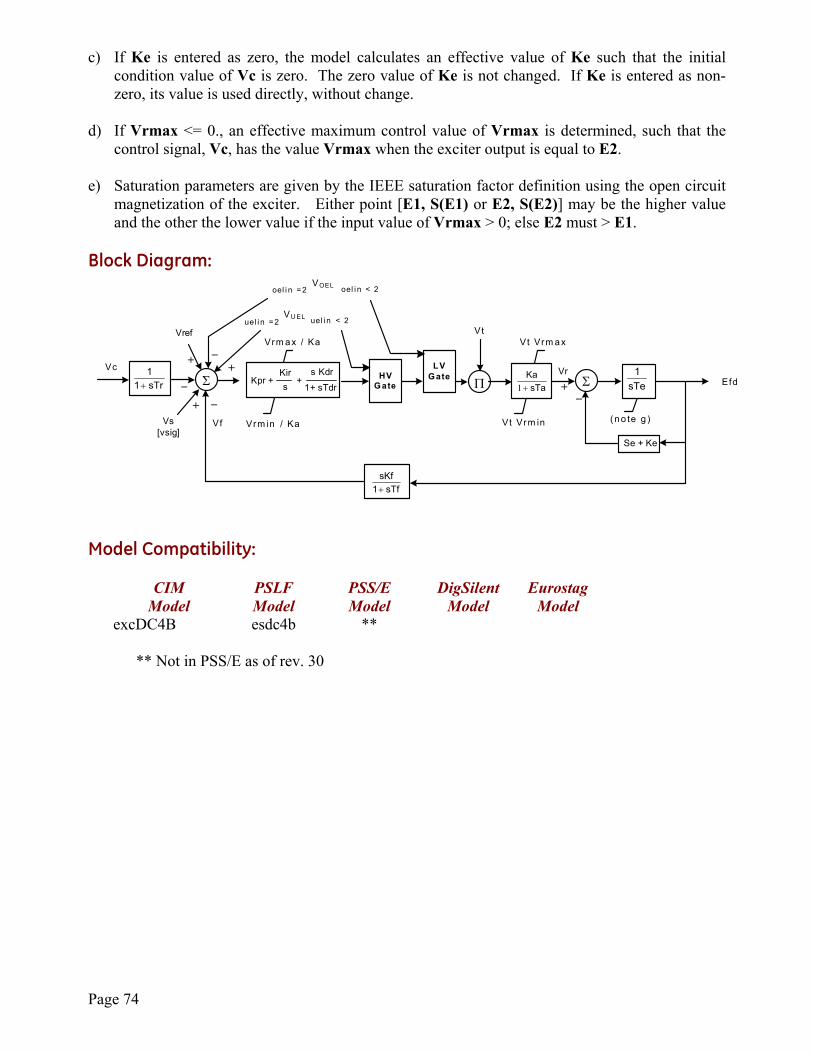
Page 74
c) If Ke is entered as zero, the model calculates an effective value of Ke such that the initial condition value of Vc is zero. The zero value of Ke is not changed. If Ke is entered as non-zero, its value is used directly, without change.
d) If Vrmax <= 0., an effective maximum control value of Vrmax is determined, such that the
control signal, Vc, has the value Vrmax when the exciter output is equal to E2. e) Saturation parameters are given by the IEEE saturation factor definition using the open circuit
magnetization of the exciter. Either point [E1, S(E1) or E2, S(E2)] may be the higher value and the other the lower value if the input value of Vrmax > 0; else E2 must > E1.
Block Diagram:
S4
Efd
Se + Ke
+Vt Vrm in
+
Vt Vrm ax
Vr
sTaKa
+1 sTe1
sTf1sKf+
Vs[vsig]
−ΣHV
Gate
Vref
sTr11
+
+
Σ
−
−
VU EL
+
uel i n < 2uel i n = 2
Vc
Vf (no te g )
LVGate
Π
−Vrm ax / Ka
Vrm in / Ka
1+ sTdr
s KdrKpr +
Kirs
+
VOEL oel i n < 2oel i n = 2
Vt
Model Compatibility:
CIM PSLF PSS/E DigSilent Eurostag Model Model Model Model Model excDC4B esdc4b **
** Not in PSS/E as of rev. 30
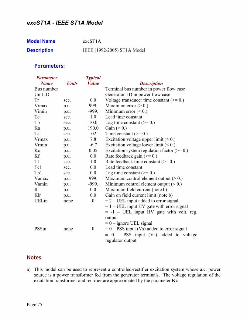
Page 75
excST1A - IEEE ST1A Model Model Name excST1A
Description IEEE (1992/2005) ST1A Model
Parameters:
Parameter Typical Name Units Value Description Bus number Terminal bus number in power flow case Unit ID Generator ID in power flow case Tr sec. 0.0 Voltage transducer time constant (>= 0.) Vimax p.u. 999. Maximum error (> 0.) Vimin p.u. -999. Minimum error (< 0.) Tc sec. 1.0 Lead time constant Tb sec. 10.0 Lag time constant (>= 0.) Ka p.u. 190.0 Gain (> 0.) Ta sec. .02 Time constant (>= 0.) Vrmax p.u. 7.8 Excitation voltage upper limit (> 0.) Vrmin p.u. -6.7 Excitation voltage lower limit (< 0.) Kc p.u. 0.05 Excitation system regulation factor (>= 0.) Kf p.u. 0.0 Rate feedback gain (>= 0.) Tf sec. 1.0 Rate feedback time constant (>= 0.) Tc1 sec. 0.0 Lead time constant Tb1 sec. 0.0 Lag time constant (>= 0.) Vamax p.u. 999. Maximum control element output (> 0.) Vamin p.u. -999. Minimum control element output (< 0.) Ilr p.u. 0.0 Maximum field current (note b) Klr p.u. 0.0 Gain on field current limit (note b) UELin none 0 = 2 – UEL input added to error signal
= 1 – UEL input HV gate with error signal = -1 – UEL input HV gate with volt. reg. output = 0 – ignore UEL signal
PSSin none 0 = 0 – PSS input (Vs) added to error signal ≠ 0 – PSS input (Vs) added to voltage regulator output
Notes: a) This model can be used to represent a controlled-rectifier excitation system whose a.c. power
source is a power transformer fed from the generator terminals. The voltage regulation of the excitation transformer and rectifier are approximated by the parameter Kc.
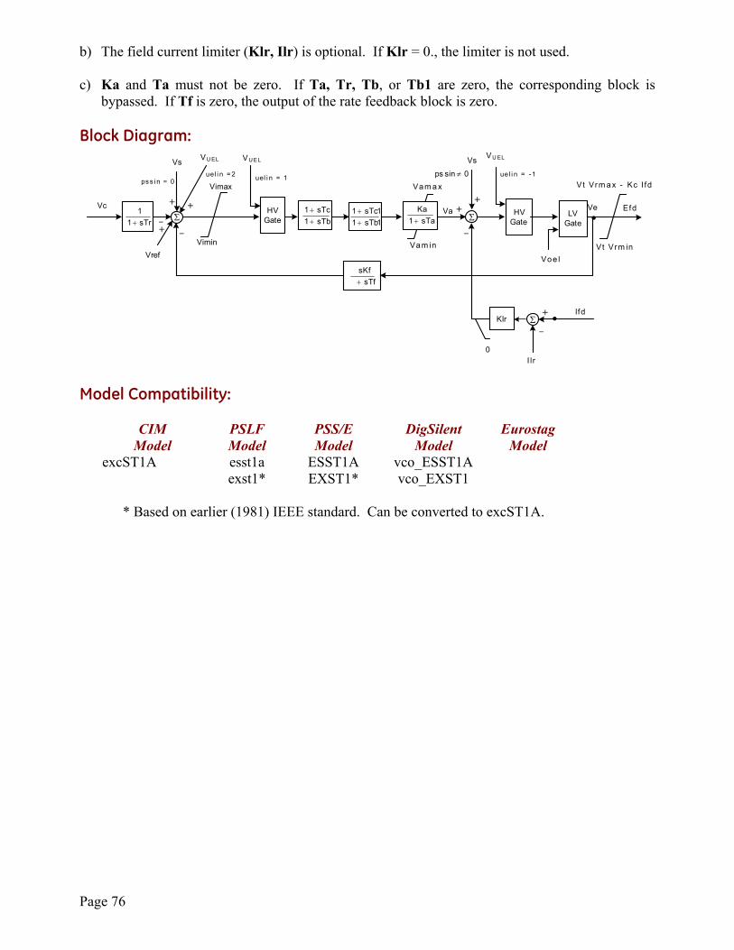
Page 76
b) The field current limiter (Klr, Ilr) is optional. If Klr = 0., the limiter is not used. c) Ka and Ta must not be zero. If Ta, Tr, Tb, or Tb1 are zero, the corresponding block is
bypassed. If Tf is zero, the output of the rate feedback block is zero.
Block Diagram:
I lr
Klr
Vam in
Vam a xVimax
Vimin
sTb1sTc1
++
1sTb11sTc1
++
Vt Vrm ax - Kc I fd
0
sTa1Ka
+sTr11
+
Vt Vrm in
sTfsKf+
Σ Σ
Σ
Vref
Vc Efd
lfd•
•++
+
+
−−
−
−
Va LVGate
HVGate
Voe l
+
VU EL
uel i n = 1uel i n = 2
HVGate
VU EL
uel i n = -1
Vs
+
ps s i n = 00sinps ≠
Vs
Ve
VU EL
Model Compatibility:
CIM PSLF PSS/E DigSilent Eurostag Model Model Model Model Model excST1A esst1a ESST1A vco_ESST1A exst1* EXST1* vco_EXST1
* Based on earlier (1981) IEEE standard. Can be converted to excST1A.
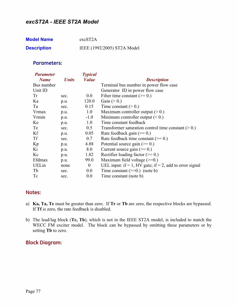
Page 77
excST2A - IEEE ST2A Model Model Name excST2A
Description IEEE (1992/2005) ST2A Model
Parameters:
Parameter Typical Name Units Value Description Bus number Terminal bus number in power flow case Unit ID Generator ID in power flow case Tr sec. 0.0 Filter time constant (>= 0.) Ka p.u. 120.0 Gain (> 0.) Ta sec. 0.15 Time constant (> 0.) Vrmax p.u. 1.0 Maximum controller output (> 0.) Vrmin p.u. -1.0 Minimum controller output (< 0.) Ke p.u. 1.0 Time constant feedback Te sec. 0.5 Transformer saturation control time constant (> 0.) Kf p.u. 0.05 Rate feedback gain (>= 0.) Tf sec. 0.7 Rate feedback time constant (>= 0.) Kp p.u. 4.88 Potential source gain (>= 0.) Ki p.u. 8.0 Current source gain (>= 0.) Kc p.u. 1.82 Rectifier loading factor (>= 0.) Efdmax p.u. 99.0 Maximum field voltage (>=0.) UELin none 0 UEL input: if = 1, HV gate; if = 2, add to error signal Tb sec. 0.0 Time constant (>=0.) (note b) Tc sec. 0.0 Time constant (note b) Notes: a) Ka, Ta, Te must be greater than zero. If Tr or Tb are zero, the respective blocks are bypassed.
If Tf is zero, the rate feedback is disabled. b) The lead/lag block (Tc, Tb), which is not in the IEEE ST2A model, is included to match the
WECC FM exciter model. The block can be bypassed by omitting these parameters or by setting Tb to zero.
Block Diagram:
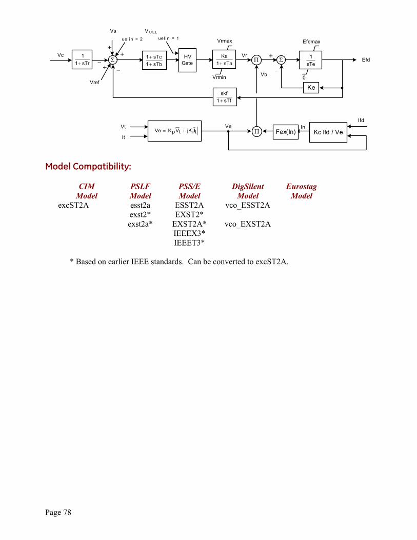
Page 78
ΠΣ Efd
Vref0
Efdmax
sTr11
+ sTe1
Vt
ItFex(In) Kc Ifd / Ve
Vrmin
Vrmax
sTa1Ka
+
Ve
Ke
sTf1skf+
Vs
Π
Σ
Ifd
tIijKtVpKVe +=
Vc Vr
Vb
In•
•
V U EL
uel i n = 1
HVGate
uel i n = 2
sTb1sTc1
++ +
+
++
−−
−
Model Compatibility:
CIM PSLF PSS/E DigSilent Eurostag Model Model Model Model Model excST2A esst2a ESST2A vco_ESST2A exst2* EXST2* exst2a* EXST2A* vco_EXST2A IEEEX3* IEEET3*
* Based on earlier IEEE standards. Can be converted to excST2A.
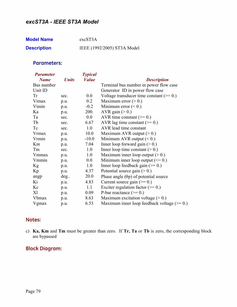
Page 79
excST3A - IEEE ST3A Model Model Name excST3A
Description IEEE (1992/2005) ST3A Model
Parameters:
Parameter Typical Name Units Value Description Bus number Terminal bus number in power flow case Unit ID Generator ID in power flow case Tr sec. 0.0 Voltage transducer time constant (>= 0.) Vimax p.u. 0.2 Maximum error (> 0.) Vimin p.u. -0.2 Minimum error (< 0.) Ka p.u. 200. AVR gain (> 0.) Ta sec. 0.0 AVR time constant (>= 0.) Tb sec. 6.67 AVR lag time constant (>= 0.) Tc sec. 1.0 AVR lead time constant Vrmax p.u. 10.0 Maximum AVR output (> 0.) Vrmin p.u. -10.0 Minimum AVR output (< 0.) Km p.u. 7.04 Inner loop forward gain (> 0.) Tm sec. 1.0 Inner loop time constant (> 0.) Vmmax p.u. 1.0 Maximum inner loop output (> 0.) Vmmin p.u. 0.0 Minimum inner loop output (<= 0.) Kg p.u. 1.0 Inner loop feedback gain (>= 0.) Kp p.u. 4.37 Potential source gain (> 0.) angp deg.. 20.0 Phase angle (θp) of potential source Ki p.u. 4.83 Current source gain (>= 0.) Kc p.u. 1.1 Exciter regulation factor (>= 0.) Xl p.u. 0.09 P-bar reactance (>= 0.) Vbmax p.u. 8.63 Maximum excitation voltage (> 0.) Vgmax p.u. 6.53 Maximum inner loop feedback voltage (>= 0.) Notes: c) Ka, Km and Tm must be greater than zero. If Tr, Ta or Tb is zero, the corresponding block
are bypassed Block Diagram:
Page 80
Vgmax
Ifd
Vs
sTr11
+
Vt
ItFex(In) Kc Ifd / Ve
Vmmin
Vmmax
sTm1Km
+
VetI)lXpKiK(jtVpK ++
Vimax
Vimin
sTb1sTc1
++
Vbmax
Kg
pjepKpK
θ=
ΣΣ
Π
Π
Vref
Efd
Vb
In
Vc•
•
Vr Vm
++
+ −
−
Vrmin
Vrmax
sTa1Ka
+HV
Gate
Vuel
Vi
Model Compatibility:
CIM PSLF PSS/E DigSilent Eurostag Model Model Model Model Model excST3A esst3a ESST3A vco_ESST3A exst3* exst3a* EXST3A* * Based on earlier IEEE standard. Can be converted to excST3A.
Page 81
excST4B - IEEE ST4B Model Model Name excST4B
Description IEEE (2005) ST4B Model
Parameters:
Parameter Typical Name Units Value Description Bus number Terminal bus number in power flow case Unit ID Generator ID in power flow case Tr sec. 0.0 Voltage transducer time constant (>= 0.) Kpr p.u. 10.75 AVR proportional gain (note b) Kir p.u. 10.75 AVR Integral gain (note b) Ta sec. 0.02 AVR time constant (>= 0.) Vrmax p.u. 1.0 Maximum AVR output (> 0.) Vrmin p.u. -0.87 Minimum AVR output (< 0.) Kpm p.u. 1.0 Prop. gain of inner loop regulator (note a) Kim p.u. 0.0 Integral gain of inner loop regulator (note a) Vmmax p.u. 99. Maximum inner loop regulator output Vmmin p.u. -99. Minimum inner loop regulator output Kg p.u. 0.0 Inner loop feedback gain (>= 0.) Kp p.u. 9.3 Potential source gain (> 0.) Angp deg.. 0.0 Phase angle (θp) of potential source Ki p.u. 0.0 Current source gain (>= 0.) Kc p.u. 0.113 Exciter regulation factor (>= 0.) Xl p.u. 0.124 P-bar leakage reactance (>= 0.) Vbmax p.u. 11.63 Maximum excitation voltage (> 0.) Vgmax p.u. 999. Maximum inner loop feedback gain (>= 0.) Notes: a) The inner loop field voltage regulator parameters (Kpm, Kim and Kg) are used for modeling of
a compound power source static exciter. Any of these values can be zero, but either Kpm or Kim must be non-zero. To bypass the inner loop field voltage regulator, set Kpm = 1.0, and Kim and Kg to zero.
b) Either of the automatic voltage regulator AVR parameters (Kpr, Kir) may be zero but at least
one must be non-zero. c) Setting Ta or Tr to zero will bypass the corresponding block. If Ta is zero, a one time step
delay is included for this block.
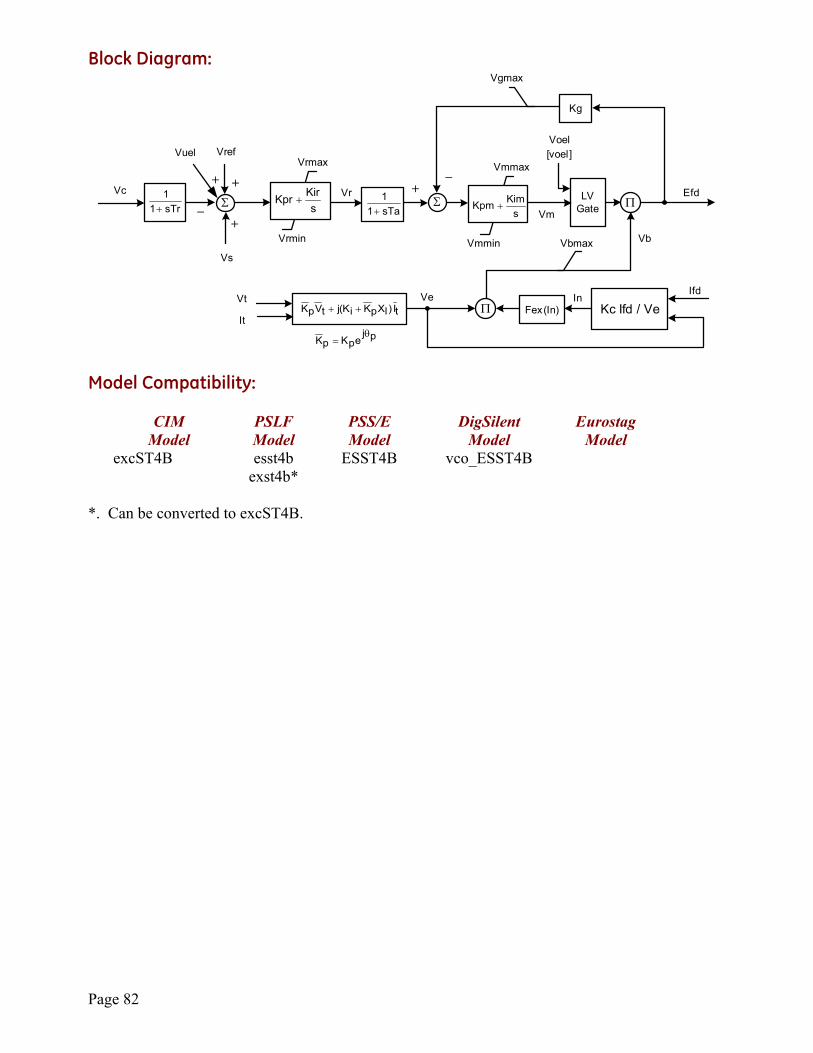
Page 82
Block Diagram: Vgmax
Ifd
Vs
sTr11
+
Vt
ItFex(In) Kc Ifd / Ve
Vmmin
Vmmax
VetI)lXpKiK(jtVpK ++
Vbmax
Kg
pjepKpK
θ=
ΣΣ
Π
Π
Vref
Efd
Vb
In
Vc•
•
Vr
Vm
+
+
+ −
−
Vrmin
Vrmax
sTa11
+
[voel]Voel
sKirKpr +
sKimKpm +
LVGate
Vuel
+
Model Compatibility:
CIM PSLF PSS/E DigSilent Eurostag Model Model Model Model Model excST4B esst4b ESST4B vco_ESST4B exst4b* *. Can be converted to excST4B.
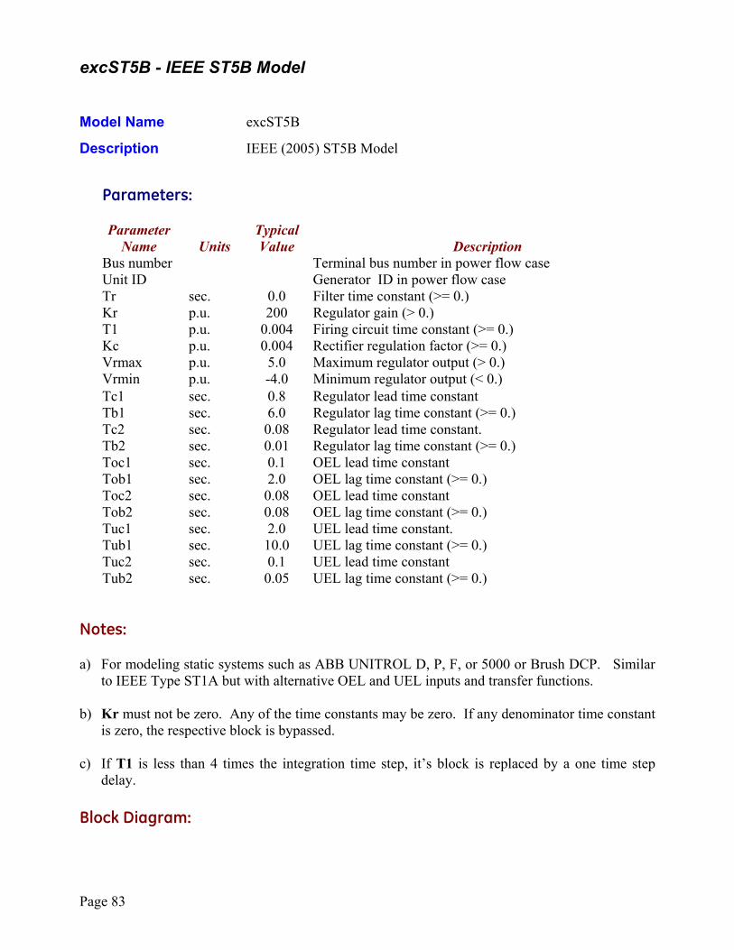
Page 83
excST5B - IEEE ST5B Model Model Name excST5B
Description IEEE (2005) ST5B Model
Parameters:
Parameter Typical Name Units Value Description Bus number Terminal bus number in power flow case Unit ID Generator ID in power flow case Tr sec. 0.0 Filter time constant (>= 0.) Kr p.u. 200 Regulator gain (> 0.) T1 p.u. 0.004 Firing circuit time constant (>= 0.) Kc p.u. 0.004 Rectifier regulation factor (>= 0.) Vrmax p.u. 5.0 Maximum regulator output (> 0.) Vrmin p.u. -4.0 Minimum regulator output (< 0.) Tc1 sec. 0.8 Regulator lead time constant Tb1 sec. 6.0 Regulator lag time constant (>= 0.) Tc2 sec. 0.08 Regulator lead time constant. Tb2 sec. 0.01 Regulator lag time constant (>= 0.) Toc1 sec. 0.1 OEL lead time constant Tob1 sec. 2.0 OEL lag time constant (>= 0.) Toc2 sec. 0.08 OEL lead time constant Tob2 sec. 0.08 OEL lag time constant (>= 0.) Tuc1 sec. 2.0 UEL lead time constant. Tub1 sec. 10.0 UEL lag time constant (>= 0.) Tuc2 sec. 0.1 UEL lead time constant Tub2 sec. 0.05 UEL lag time constant (>= 0.) Notes: a) For modeling static systems such as ABB UNITROL D, P, F, or 5000 or Brush DCP. Similar
to IEEE Type ST1A but with alternative OEL and UEL inputs and transfer functions. b) Kr must not be zero. Any of the time constants may be zero. If any denominator time constant
is zero, the respective block is bypassed. c) If T1 is less than 4 times the integration time step, it’s block is replaced by a one time step
delay. Block Diagram:
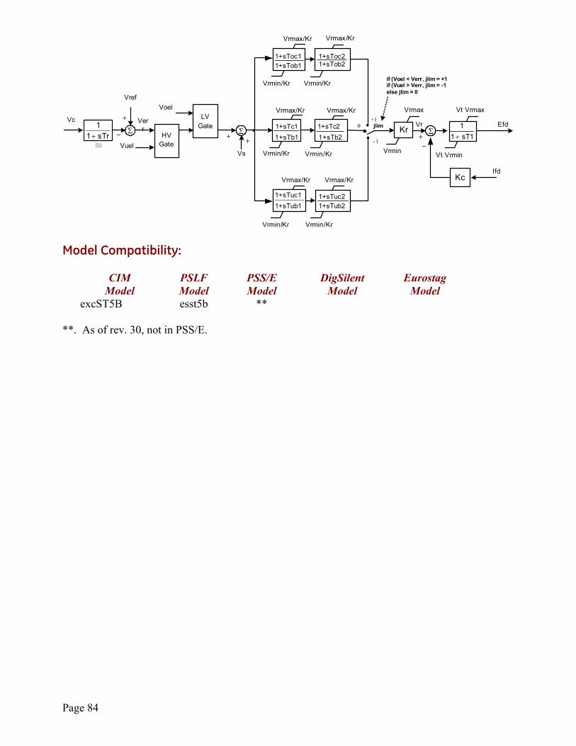
Page 84
1sT11
+
Kc
Efd
S0
Vc +
Vref
Vrmin
+
Vrmax
Kr+
Vt Vrmax
sTr11
+
Vt VrminVs
•− Σ
Ifd
Vrmax/Kr
Vrmin/Kr
Vrmax/Kr
Vrmin/Kr
ΣΣ •HV
GateVuel
LVGate
Voel
Vrmax/Kr
Vrmin/Kr
+−
0+1
−1
jlim
if (Voel < Verr, jlim = +1if (Vuel > Verr, jlim = -1else jlim = 0
Verr
Vrmin/Kr
Vrmax/Kr
Vrmin/Kr
Vrmax/Kr
Vrmax/Kr
Vrmin/Kr
Vr
1+sTuc11+sTub1
1+sTob11+sToc1
1+sTc21+sTb21+sTb1
1+sTc1
1+sTub21+sTuc2
1+sToc21+sTob2
Model Compatibility:
CIM PSLF PSS/E DigSilent Eurostag Model Model Model Model Model excST5B esst5b ** **. As of rev. 30, not in PSS/E.
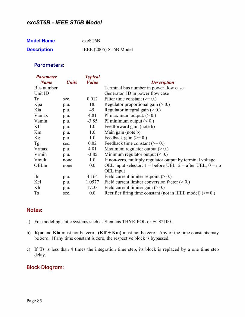
Page 85
excST6B - IEEE ST6B Model Model Name excST6B
Description IEEE (2005) ST6B Model
Parameters:
Parameter Typical Name Units Value Description Bus number Terminal bus number in power flow case Unit ID Generator ID in power flow case Tr sec. 0.012 Filter time constant (>= 0.) Kpa p.u. 18. Regulator proportional gain (> 0.) Kia p.u. 45. Regulator integral gain (> 0.) Vamax p.u. 4.81 PI maximum output. (> 0.) Vamin p.u. -3.85 PI minimum output (< 0.) Kff p.u. 1.0 Feedforward gain (note b) Km p.u. 1.0 Main gain (note b) Kg p.u. 1.0 Feedback gain (>= 0.) Tg sec. 0.02 Feedback time constant (>= 0.) Vrmax p.u. 4.81 Maximum regulator output (> 0.) Vrmin p.u. -3.85 Minimum regulator output (< 0.) Vmult none 1.0 If non-zero, multiply regulator output by terminal voltage OELin none 0.0 OEL input selector: 1 – before UEL, 2 – after UEL, 0 – no
OEL input Ilr p.u. 4.164 Field current limiter setpoint (> 0.) Kcl p.u. 1.0577 Field current limiter conversion factor (> 0.) Klr p.u. 17.33 Field current limiter gain (> 0.) Ts sec. 0.0 Rectifier firing time constant (not in IEEE model) (>= 0.) Notes: a) For modeling static systems such as Siemens THYRIPOL or ECS2100. b) Kpa and Kia must not be zero. (Kff + Km) must not be zero. Any of the time constants may
be zero. If any time constant is zero, the respective block is bypassed. c) If Ts is less than 4 times the integration time step, its block is replaced by a one time step
delay. Block Diagram:
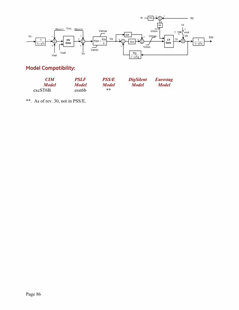
Page 86
EfdVc +
Vrmin
+
+
Vs
−
Σ •
sTgKg
+1
Vrmax+
sKiaKpa +Σ
+
−
Vamax
Vamin
KmΣ Σ+
−
Kff
LVGate
vmult1
01
Vt
Ilr
Klr
Ifd+
Kcl
Vrmin
−
VrVa•HV
GatesTr11
+
Vref
−
Vuel
VOELOELin=1 OELin=2
Vb
Π
Σ
sTs11
+
Model Compatibility:
CIM PSLF PSS/E DigSilent Eurostag Model Model Model Model Model excST6B esst6b ** **. As of rev. 30, not in PSS/E.
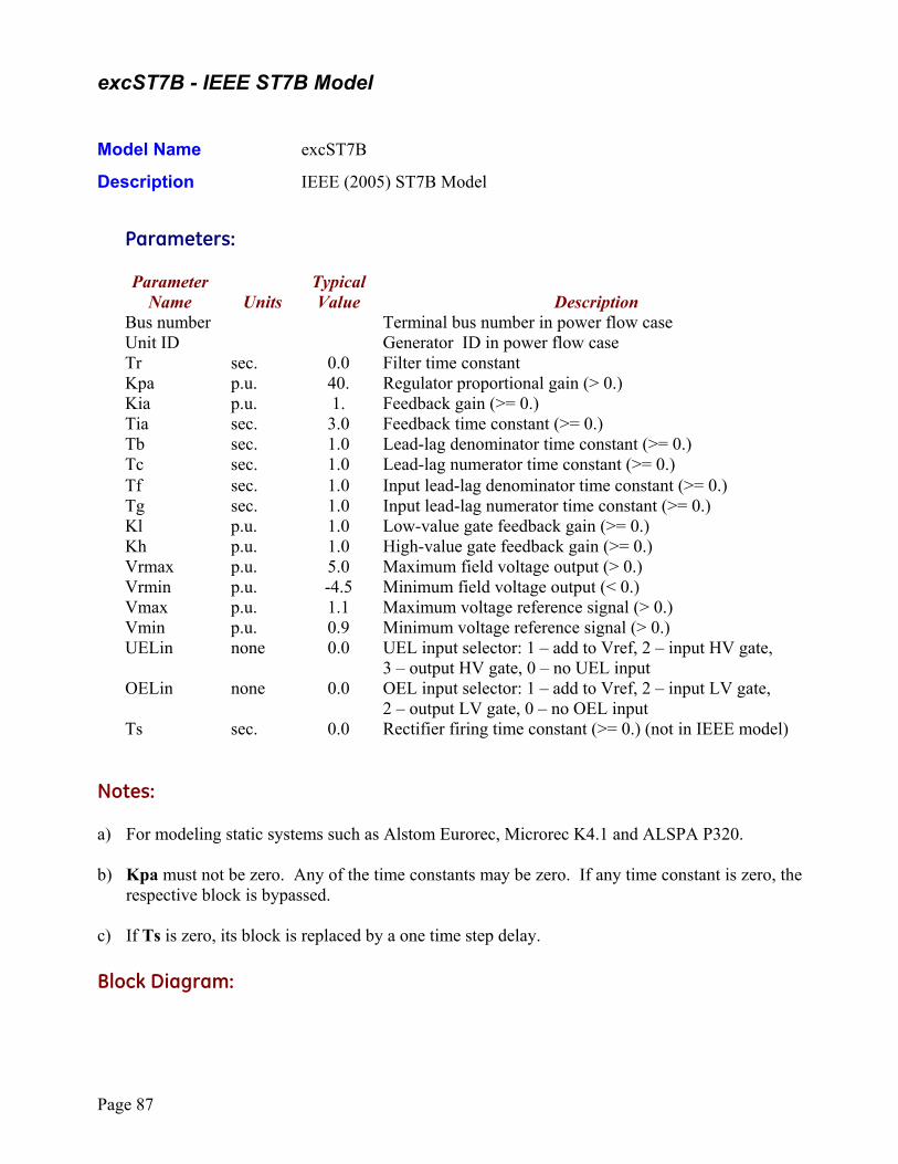
Page 87
excST7B - IEEE ST7B Model Model Name excST7B
Description IEEE (2005) ST7B Model
Parameters:
Parameter Typical Name Units Value Description Bus number Terminal bus number in power flow case Unit ID Generator ID in power flow case Tr sec. 0.0 Filter time constant Kpa p.u. 40. Regulator proportional gain (> 0.) Kia p.u. 1. Feedback gain (>= 0.) Tia sec. 3.0 Feedback time constant (>= 0.) Tb sec. 1.0 Lead-lag denominator time constant (>= 0.) Tc sec. 1.0 Lead-lag numerator time constant (>= 0.) Tf sec. 1.0 Input lead-lag denominator time constant (>= 0.) Tg sec. 1.0 Input lead-lag numerator time constant (>= 0.) Kl p.u. 1.0 Low-value gate feedback gain (>= 0.) Kh p.u. 1.0 High-value gate feedback gain (>= 0.) Vrmax p.u. 5.0 Maximum field voltage output (> 0.) Vrmin p.u. -4.5 Minimum field voltage output (< 0.) Vmax p.u. 1.1 Maximum voltage reference signal (> 0.) Vmin p.u. 0.9 Minimum voltage reference signal (> 0.) UELin none 0.0 UEL input selector: 1 – add to Vref, 2 – input HV gate,
3 – output HV gate, 0 – no UEL input OELin none 0.0 OEL input selector: 1 – add to Vref, 2 – input LV gate,
2 – output LV gate, 0 – no OEL input Ts sec. 0.0 Rectifier firing time constant (>= 0.) (not in IEEE model) Notes: a) For modeling static systems such as Alstom Eurorec, Microrec K4.1 and ALSPA P320. b) Kpa must not be zero. Any of the time constants may be zero. If any time constant is zero, the
respective block is bypassed. c) If Ts is zero, its block is replaced by a one time step delay. Block Diagram:
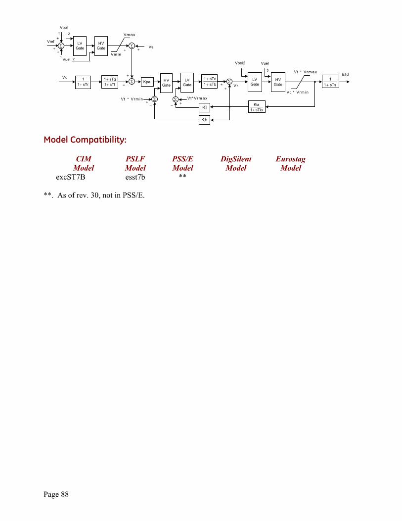
Page 88
Kpa
EfdVc
+sTb1sTc1
++
sTs11
+sTr11
+
Vt * Vrm in
sTf1sTg1
++
+
VrefVs
−Σ
sTia1Kia
+
Vt * Vrm ax
+HV
GateLV
GateLV
GateHV
Gate
Kl
Σ
Σ Vt* Vrm ax+−
Σ
Kh
Vt * Vrm in−
+
Σ+
Vm in
Vm ax
HVGate
LVGateΣ
Voel
Vuel
+ ++
+
VuelVoel21 2
1 2
3
Vr•
•
Model Compatibility:
CIM PSLF PSS/E DigSilent Eurostag Model Model Model Model Model excST7B esst7b ** **. As of rev. 30, not in PSS/E.
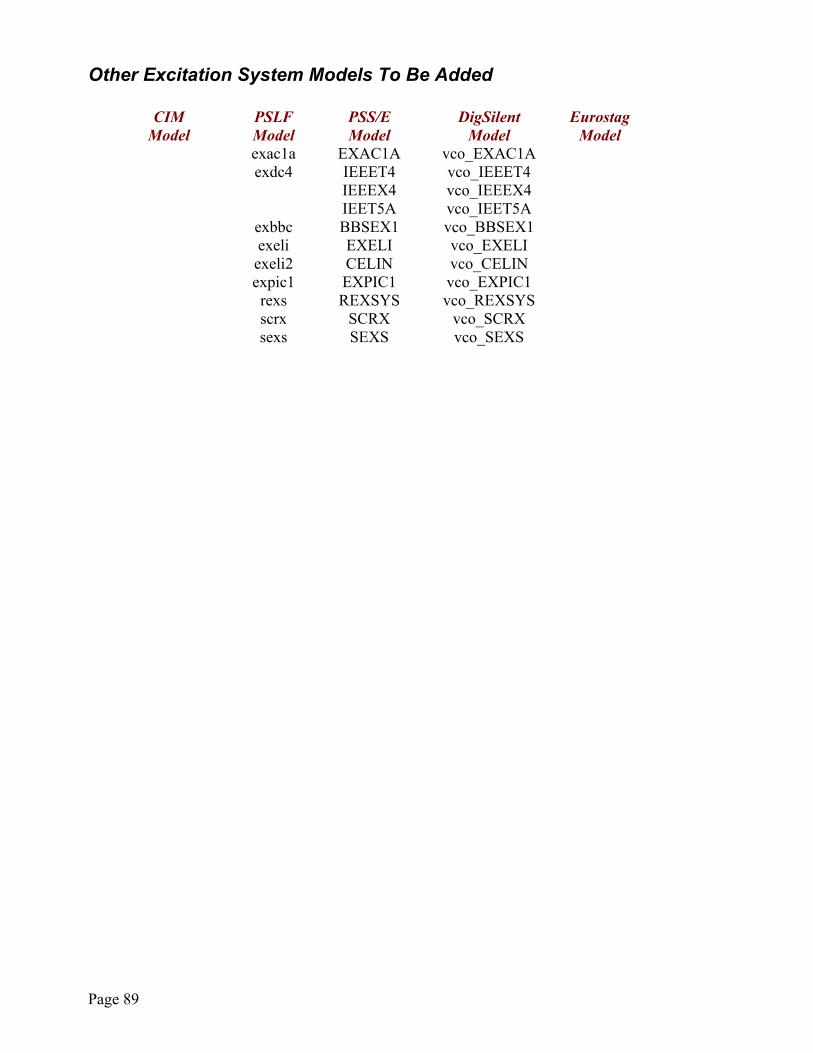
Page 89
Other Excitation System Models To Be Added CIM PSLF PSS/E DigSilent Eurostag Model Model Model Model Model exac1a EXAC1A vco_EXAC1A exdc4 IEEET4
IEEEX4 vco_IEEET4 vco_IEEEX4
IEET5A vco_IEET5A exbbc BBSEX1 vco_BBSEX1 exeli EXELI vco_EXELI exeli2 CELIN vco_CELIN expic1 EXPIC1 vco_EXPIC1 rexs REXSYS vco_REXSYS scrx SCRX vco_SCRX sexs SEXS vco_SEXS
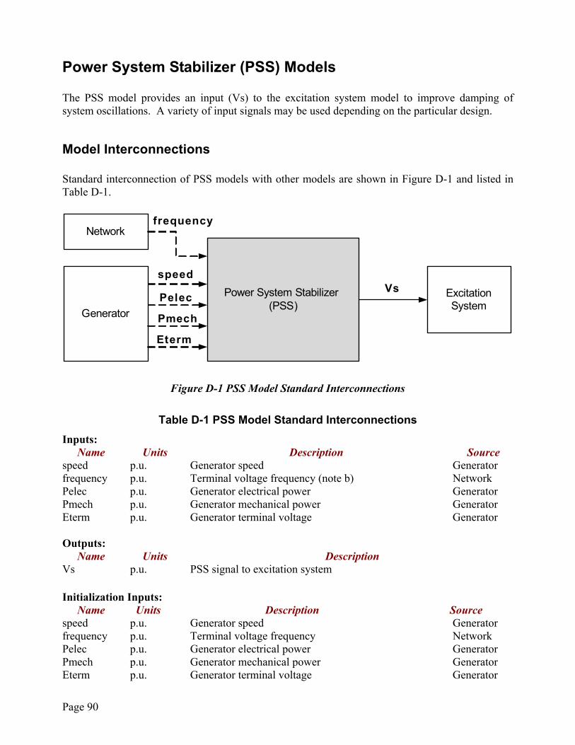
Page 90
Power System Stabilizer (PSS) Models The PSS model provides an input (Vs) to the excitation system model to improve damping of system oscillations. A variety of input signals may be used depending on the particular design.
Model Interconnections Standard interconnection of PSS models with other models are shown in Figure D-1 and listed in Table D-1.
VsPower System Stabilizer (PSS)
Excitation System
speed
Networkfrequency
GeneratorPelec
Eterm
Pmech
Figure D-1 PSS Model Standard Interconnections
Table D-1 PSS Model Standard Interconnections Inputs:
Name Units Description Source speed p.u. Generator speed Generator frequency p.u. Terminal voltage frequency (note b) Network Pelec p.u. Generator electrical power Generator Pmech p.u. Generator mechanical power Generator Eterm p.u. Generator terminal voltage Generator Outputs:
Name Units Description Vs p.u. PSS signal to excitation system Initialization Inputs:
Name Units Description Source speed p.u. Generator speed Generator frequency p.u. Terminal voltage frequency Network Pelec p.u. Generator electrical power Generator Pmech p.u. Generator mechanical power Generator Eterm p.u. Generator terminal voltage Generator
Page 91
Vs p.u. PSS signal to excitation system (note a) Exc. System Notes: a) Vs is always initialized to zero by the excitation system model. b) If bus voltage frequency is not available from network, the model can calculate it as derivative
of the bus voltage angle.
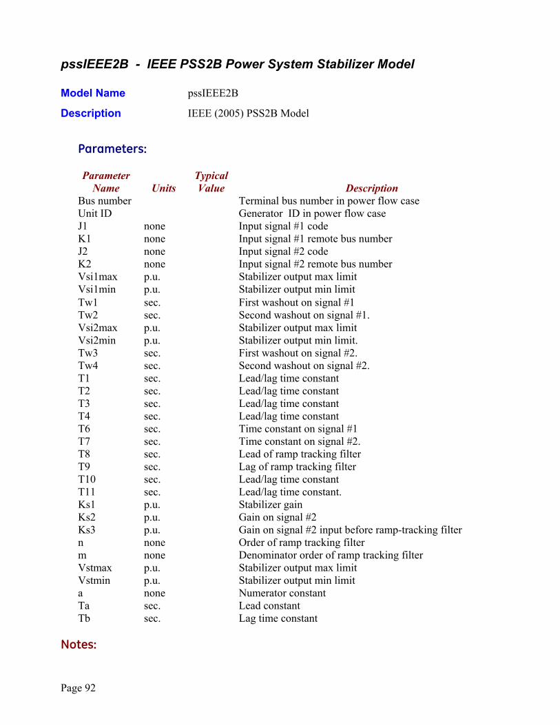
Page 92
pssIEEE2B - IEEE PSS2B Power System Stabilizer Model Model Name pssIEEE2B
Description IEEE (2005) PSS2B Model
Parameters:
Parameter Typical Name Units Value Description Bus number Terminal bus number in power flow case Unit ID Generator ID in power flow case J1 none Input signal #1 code K1 none Input signal #1 remote bus number J2 none Input signal #2 code K2 none Input signal #2 remote bus number Vsi1max p.u. Stabilizer output max limit Vsi1min p.u. Stabilizer output min limit Tw1 sec. First washout on signal #1 Tw2 sec. Second washout on signal #1. Vsi2max p.u. Stabilizer output max limit Vsi2min p.u. Stabilizer output min limit. Tw3 sec. First washout on signal #2. Tw4 sec. Second washout on signal #2. T1 sec. Lead/lag time constant T2 sec. Lead/lag time constant T3 sec. Lead/lag time constant T4 sec. Lead/lag time constant T6 sec. Time constant on signal #1 T7 sec. Time constant on signal #2. T8 sec. Lead of ramp tracking filter T9 sec. Lag of ramp tracking filter T10 sec. Lead/lag time constant T11 sec. Lead/lag time constant. Ks1 p.u. Stabilizer gain Ks2 p.u. Gain on signal #2 Ks3 p.u. Gain on signal #2 input before ramp-tracking filter n none Order of ramp tracking filter m none Denominator order of ramp tracking filter Vstmax p.u. Stabilizer output max limit Vstmin p.u. Stabilizer output min limit a none Numerator constant Ta sec. Lead constant Tb sec. Lag time constant Notes:
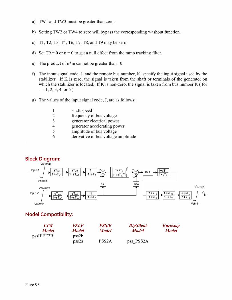
Page 93
a) TW1 and TW3 must be greater than zero.
b) Setting TW2 or TW4 to zero will bypass the corresponding washout function.
c) T1, T2, T3, T4, T6, T7, T8, and T9 may be zero.
d) Set T9 = 0 or n = 0 to get a null effect from the ramp tracking filter.
e) The product of n*m cannot be greater than 10.
f) The input signal code, J, and the remote bus number, K, specify the input signal used by the
stabilizer. If K is zero, the signal is taken from the shaft or terminals of the generator on which the stabilizer is located. If K is non-zero, the signal is taken from bus number K ( for J = 1, 2, 3, 4, or 5 ).
g) The values of the input signal code, J, are as follows:
1 shaft speed 2 frequency of bus voltage 3 generator electrical power 4 generator accelerating power 5 amplitude of bus voltage 6 derivative of bus voltage amplitude
. Block Diagram:
Ks1
Ks3 Ks4Vstmax
Vstmin
Vs
Vsi2min
Vsi1max
Vsi1min
Input 1
Input 2
Σ Σ 1+sT2
a+sTa1+sTb
sTw2
1+sTw2
1+sT7
11+sT6
1+sT11
1+sT10
1+sT4
1+sT3
1+sT1
1
sTw1
1+sTw1
sTw31+sTw3
sTw41+sTw4
Vsi2max
( )
n
m9
8sT1sT1
+
+
Model Compatibility:
CIM PSLF PSS/E DigSilent Eurostag Model Model Model Model Model pssIEEE2B pss2b pss2a PSS2A pss_PSS2A
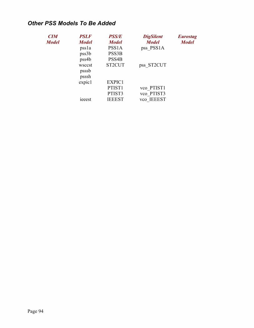
Page 94
Other PSS Models To Be Added CIM PSLF PSS/E DigSilent Eurostag Model Model Model Model Model pss1a PSS1A pss_PSS1A pss3b PSS3B pss4b PSS4B wsccst ST2CUT pss_ST2CUT psssb psssh expic1 EXPIC1 PTIST1 vco_PTIST1 PTIST3 vco_PTIST3 ieeest IEEEST vco_IEEEST
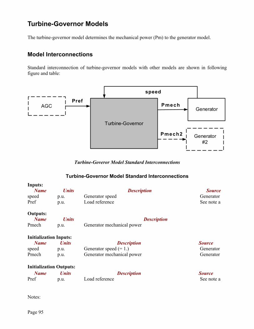
Page 95
Turbine-Governor Models The turbine-governor model determines the mechanical power (Pm) to the generator model.
Model Interconnections Standard interconnection of turbine-governor models with other models are shown in following figure and table:
Pmech
speed
Pref
Turbine-Governor
GeneratorAGC
Generator#2
Pmech2
Turbine-Goveror Model Standard Interconnections
Turbine-Governor Model Standard Interconnections Inputs:
Name Units Description Source speed p.u. Generator speed Generator Pref p.u. Load reference See note a Outputs:
Name Units Description Pmech p.u. Generator mechanical power Initialization Inputs:
Name Units Description Source speed p.u. Generator speed (= 1.) Generator Pmech p.u. Generator mechanical power Generator Initialization Outputs:
Name Units Description Source Pref p.u. Load reference See note a Notes:

Page 96
a) Pref is usually held constant for stability analysis, but may be deteremined by a user-written model or, for long-term dynamics, an area-wide automatic generation control (AGC) model.
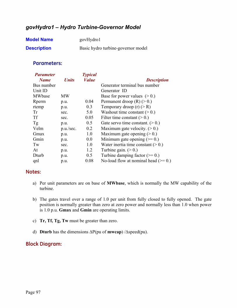
Page 97
govHydro1 – Hydro Turbine-Governor Model Model Name govHydro1
Description Basic hydro turbine-governor model
Parameters:
Parameter Typical Name Units Value Description Bus number Generator terminal bus number Unit ID Generator ID MWbase MW Base for power values (> 0.) Rperm p.u. 0.04 Permanent droop (R) (> 0.) rtemp p.u. 0.3 Temporary droop (r) (> R) Tr sec. 5.0 Washout time constant (> 0.) Tf sec. 0.05 Filter time constant (> 0.) Tg p.u. 0.5 Gate servo time constant. (> 0.) Velm p.u./sec. 0.2 Maximum gate velocity. (> 0.) Gmax p.u. 1.0 Maximum gate opening (> 0.) Gmin p.u. 0.0 Minimum gate opening (>= 0.) Tw sec. 1.0 Water inertia time constant (> 0.) At p.u. 1.2 Turbine gain. (> 0.) Dturb p.u. 0.5 Turbine damping factor (>= 0.) qnl p.u. 0.08 No-load flow at nominal head (>= 0.) Notes:
a) Per unit parameters are on base of MWbase, which is normally the MW capability of the turbine.
b) The gates travel over a range of 1.0 per unit from fully closed to fully opened. The gate position is normally greater than zero at zero power and normally less than 1.0 when power is 1.0 p.u. Gmax and Gmin are operating limits.
c) Tr, Tf, Tg, Tw must be greater than zero.
d) Dturb has the dimensions ∆P(pu of mwcap) /∆speed(pu). Block Diagram:
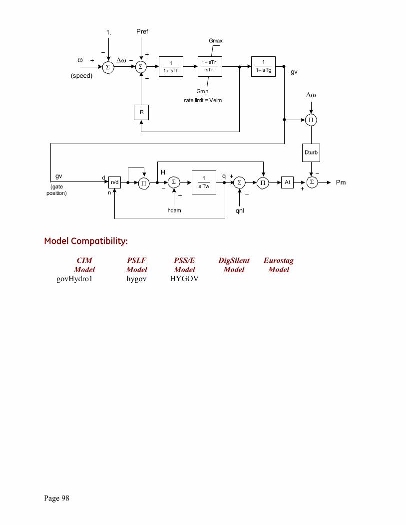
Page 98
Pref
rsTrsTr1 +
Σ
sTf11
+
Dturb
sTg11
+
Atn/d ΣTws1
Pm
hdam qnl
Gmin
Gmax
R
rate limit = Velmω∆
gv(gate
position)
qH•
•
•gv
ω
•
•
•
1.
ω∆
n
d
(speed)Σ Σ
Π
Π
Π Σ
Model Compatibility:
CIM PSLF PSS/E DigSilent Eurostag Model Model Model Model Model govHydro1 hygov HYGOV
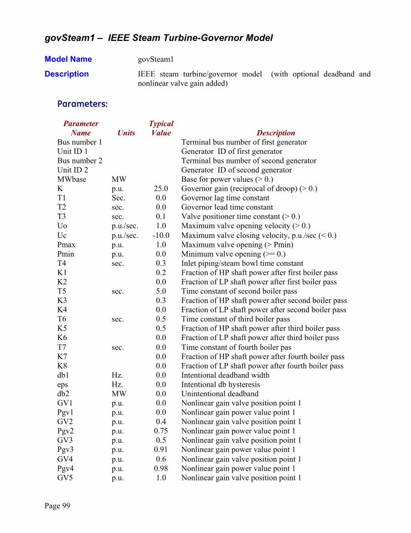
Page 99
govSteam1 – IEEE Steam Turbine-Governor Model Model Name govSteam1
Description IEEE steam turbine/governor model (with optional deadband and nonlinear valve gain added)
Parameters:
Parameter Typical Name Units Value Description Bus number 1 Terminal bus number of first generator Unit ID 1 Generator ID of first generator Bus number 2 Terminal bus number of second generator Unit ID 2 Generator ID of second generator MWbase MW Base for power values (> 0.) K p.u. 25.0 Governor gain (reciprocal of droop) (> 0.) T1 Sec. 0.0 Governor lag time constant T2 sec. 0.0 Governor lead time constant T3 sec. 0.1 Valve positioner time constant (> 0.) Uo p.u./sec. 1.0 Maximum valve opening velocity (> 0.) Uc p.u./sec. -10.0 Maximum valve closing velocity, p.u./sec (< 0.) Pmax p.u. 1.0 Maximum valve opening (> Pmin) Pmin p.u. 0.0 Minimum valve opening (>= 0.) T4 sec. 0.3 Inlet piping/steam bowl time constant K1 0.2 Fraction of HP shaft power after first boiler pass K2 0.0 Fraction of LP shaft power after first boiler pass T5 sec. 5.0 Time constant of second boiler pass K3 0.3 Fraction of HP shaft power after second boiler pass K4 0.0 Fraction of LP shaft power after second boiler pass T6 sec. 0.5 Time constant of third boiler pass K5 0.5 Fraction of HP shaft power after third boiler pass K6 0.0 Fraction of LP shaft power after third boiler pass T7 sec. 0.0 Time constant of fourth boiler pas K7 0.0 Fraction of HP shaft power after fourth boiler pass K8 0.0 Fraction of LP shaft power after fourth boiler pass db1 Hz. 0.0 Intentional deadband width eps Hz. 0.0 Intentional db hysteresis db2 MW 0.0 Unintentional deadband GV1 p.u. 0.0 Nonlinear gain valve position point 1 Pgv1 p.u. 0.0 Nonlinear gain power value point 1 GV2 p.u. 0.4 Nonlinear gain valve position point 1 Pgv2 p.u. 0.75 Nonlinear gain power value point 1 GV3 p.u. 0.5 Nonlinear gain valve position point 1 Pgv3 p.u. 0.91 Nonlinear gain power value point 1 GV4 p.u. 0.6 Nonlinear gain valve position point 1 Pgv4 p.u. 0.98 Nonlinear gain power value point 1 GV5 p.u. 1.0 Nonlinear gain valve position point 1
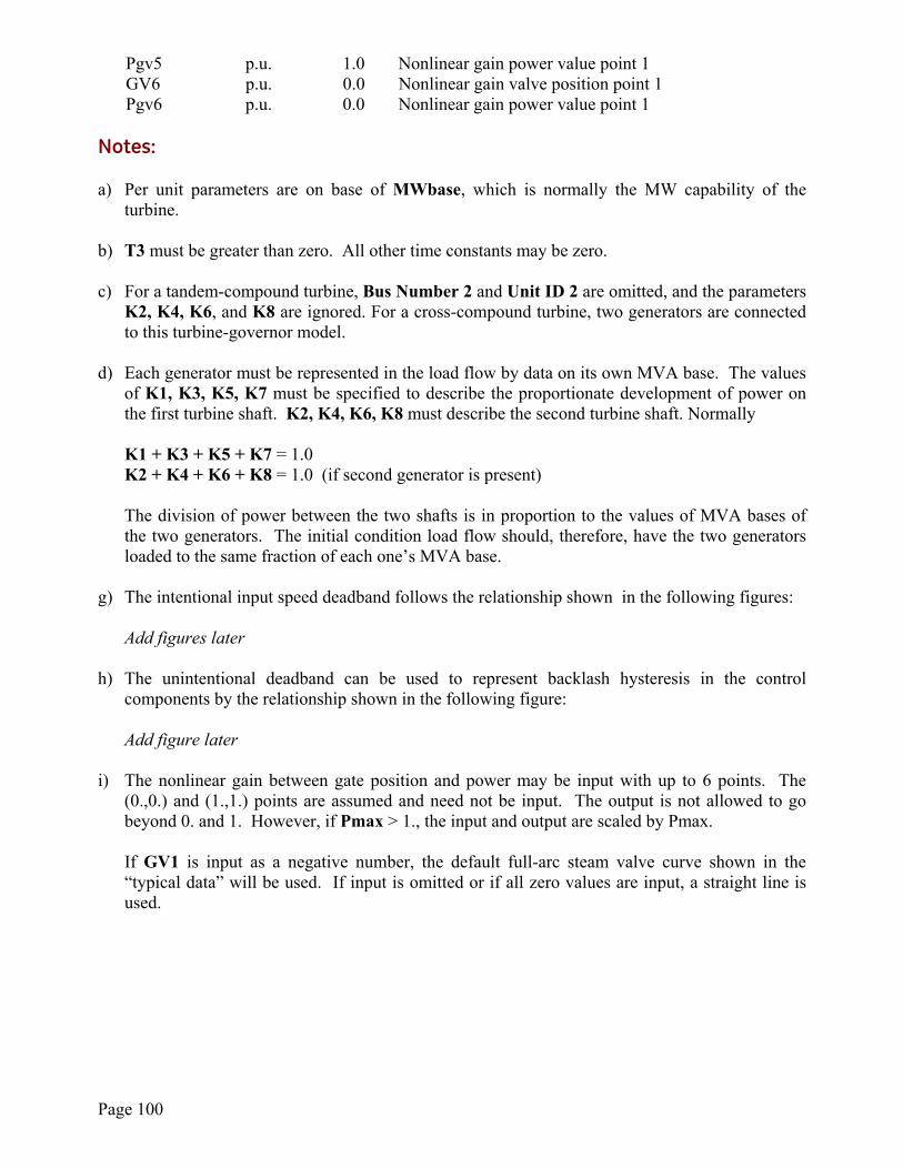
Page 100
Pgv5 p.u. 1.0 Nonlinear gain power value point 1 GV6 p.u. 0.0 Nonlinear gain valve position point 1 Pgv6 p.u. 0.0 Nonlinear gain power value point 1 Notes: a) Per unit parameters are on base of MWbase, which is normally the MW capability of the
turbine. b) T3 must be greater than zero. All other time constants may be zero. c) For a tandem-compound turbine, Bus Number 2 and Unit ID 2 are omitted, and the parameters
K2, K4, K6, and K8 are ignored. For a cross-compound turbine, two generators are connected to this turbine-governor model.
d) Each generator must be represented in the load flow by data on its own MVA base. The values
of K1, K3, K5, K7 must be specified to describe the proportionate development of power on the first turbine shaft. K2, K4, K6, K8 must describe the second turbine shaft. Normally
K1 + K3 + K5 + K7 = 1.0 K2 + K4 + K6 + K8 = 1.0 (if second generator is present)
The division of power between the two shafts is in proportion to the values of MVA bases of the two generators. The initial condition load flow should, therefore, have the two generators loaded to the same fraction of each one’s MVA base.
g) The intentional input speed deadband follows the relationship shown in the following figures:
Add figures later
h) The unintentional deadband can be used to represent backlash hysteresis in the control components by the relationship shown in the following figure:
Add figure later
i) The nonlinear gain between gate position and power may be input with up to 6 points. The (0.,0.) and (1.,1.) points are assumed and need not be input. The output is not allowed to go beyond 0. and 1. However, if Pmax > 1., the input and output are scaled by Pmax.
If GV1 is input as a negative number, the default full-arc steam valve curve shown in the “typical data” will be used. If input is omitted or if all zero values are input, a straight line is used.
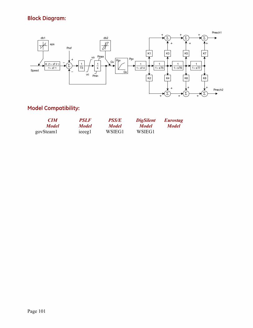
Page 101
Block Diagram:
Pgv
Σ
Pref
4sT11
+1sT1)2sT1(K
++
K1
Σ
Pmech2
Gv
db1 db2
3T1
s1
Pmin
Pmaxuo
uc
Pgv
5sT11
+
K3
6sT11
+
Σ
K5
7sT11
+
Σ
K7
K2 K4 K6 K8
Σ Σ Σ
Pmech1
Speed
Gv
eps
Model Compatibility:
CIM PSLF PSS/E DigSilent Eurostag Model Model Model Model Model govSteam1 ieeeg1 WSIEG1 WSIEG1
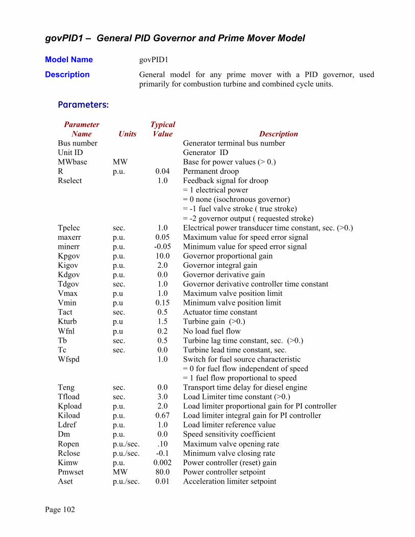
Page 102
govPID1 – General PID Governor and Prime Mover Model Model Name govPID1
Description General model for any prime mover with a PID governor, used primarily for combustion turbine and combined cycle units.
Parameters:
Parameter Typical Name Units Value Description Bus number Generator terminal bus number Unit ID Generator ID MWbase MW Base for power values (> 0.) R p.u. 0.04 Permanent droop Rselect 1.0 Feedback signal for droop = 1 electrical power = 0 none (isochronous governor) = -1 fuel valve stroke ( true stroke) = -2 governor output ( requested stroke) Tpelec sec. 1.0 Electrical power transducer time constant, sec. (>0.) maxerr p.u. 0.05 Maximum value for speed error signal minerr p.u. -0.05 Minimum value for speed error signal Kpgov p.u. 10.0 Governor proportional gain Kigov p.u. 2.0 Governor integral gain Kdgov p.u. 0.0 Governor derivative gain Tdgov sec. 1.0 Governor derivative controller time constant Vmax p.u 1.0 Maximum valve position limit Vmin p.u 0.15 Minimum valve position limit Tact sec. 0.5 Actuator time constant Kturb p.u 1.5 Turbine gain (>0.) Wfnl p.u 0.2 No load fuel flow Tb sec. 0.5 Turbine lag time constant, sec. (>0.) Tc sec. 0.0 Turbine lead time constant, sec. Wfspd 1.0 Switch for fuel source characteristic = 0 for fuel flow independent of speed = 1 fuel flow proportional to speed Teng sec. 0.0 Transport time delay for diesel engine Tfload sec. 3.0 Load Limiter time constant (>0.) Kpload p.u. 2.0 Load limiter proportional gain for PI controller Kiload p.u. 0.67 Load limiter integral gain for PI controller Ldref p.u. 1.0 Load limiter reference value Dm p.u. 0.0 Speed sensitivity coefficient Ropen p.u./sec. .10 Maximum valve opening rate Rclose p.u./sec. -0.1 Minimum valve closing rate Kimw p.u. 0.002 Power controller (reset) gain Pmwset MW 80.0 Power controller setpoint Aset p.u./sec. 0.01 Acceleration limiter setpoint
Page 103
Ka p.u. 10.0 Acceleration limiter gain Ta sec. 0.1 Acceleration limiter time constant (>0.) db p.u. 0.0 Speed governor dead band Tsa sec. 4.0 Temperature detection lead time constant Tsb sec. 5.0 Temperature detection lag time constant Rup p.u. 99.0 Maximum rate of load limit increase Rdown p.u. -99.0 Maximum rate of load limit decrease Notes: a) Per unit parameters are on base of MWbase, which is normally the MW capability of the
turbine. b) This model can be used to represent a variety of prime movers controlled by PID governors. It
is suitable, for example, for representation of • gas turbine and single shaft combined cycle turbines • diesel engines with modern electronic or digital governors • steam turbines where steam is supplied from a large boiler drum or a large header whose
pressure is substantially constant over the period under study • simple hydro turbines in dam configurations where the water column length is short and
water inertia effects are minimal c) The range of fuel valve travel and of fuel flow is unity. Thus the largest possible value of
Vmax is 1.0 and the smallest possible value of Vmin is zero. Vmax may, however, be reduced below unity to represent a loading limit that may be imposed by the operator or a supervisory control system. For gas turbines Vmin should normally be greater than zero and less than Wfnl to represent a minimum firing limit.
The value of the fuel flow at maximum output must be less than, or equal to unity, depending on the value of Kturb. If the initial power requires a fuel flow greater than 1.0, a warning message is written and Kturb is increased to permit initialization with valve position = 1.0.
d) The parameter Teng is provided for use in representing diesel engines where there is a small
but measurable transport delay between a change in fuel flow setting and the development of torque. Teng should be zero in all but special cases where this transport delay is of particular concern.
e) The parameter Wfspd is provided to recognize that fuel flow, for a given fuel valve stroke, can
be proportional to engine speed. This is the case for GE gas turbines and for diesel engines with positive displacement fuel injectors. Wfspd should be set to unity for all GE gas turbines and most diesel engines. Wfspd should be set to zero where it is known that the fuel control system keeps fuel flow independent of the engine speed.
f) The load limiter module may be used to impose a maximum output limit such as an exhaust
temperature limit. To do this the time constant Tfload should be set to represent the time constant in the measurement of temperature (or other signal), and the gains of the limiter, Kpload, Kiload, should be set to give prompt stable control when on limit. The load limit can be deactivated by setting the parameter Ldref to a high value.
Page 104
g) The parameter Dm can represent either the variation of the engine power with the shaft speed or the variation of maximum power capability with shaft speed.
If Dm is positive it describes the falling slope of the engine speed verses power characteristic as speed increases. A slightly falling characteristic is typical for reciprocating engines and some aero-derivative turbines. If Dm is negative the engine power is assumed to be unaffected by the shaft speed, but the maximum permissible fuel flow is taken to fall with falling shaft speed. This is characteristic of single-shaft industrial turbines due to exhaust temperature limits.
h) This model includes a simple representation of a supervisory load controller. This controller is active if the parameter Kimw is non-zero. The load controller is a slow acting reset loop that adjusts the speed/load reference of the turbine governor to hold the electrical power output of the unit at its initial condition value. This value is stored in the parameter Pmwset when the model is initialized, and can be changed thereafter. The load controller must be adjusted to respond gently relative to the speed governor. A typical value for Kimw is 0.01, corresponding to a reset time of 100 seconds.
i) The parameters Aset, Ka, and Ta describe an acceleration limiter. Ta must be non-zero, but
the acceleration limiter can be disabled by setting Aset to a large value, such as 1. l) The parameter, db, is the speed governor dead band. This parameter is stated in terms of per
unit speed. In the majority of applications, it is recommended that this value be set to zero. m) The parameters, Tsa, Tsb, are provided to augment the exhaust gas temperature measurement
subsystem in gas turbines. For example, they may be set to values such as 4., 5., to represent the ‘radiation shield’ element of large gas turbines. If both parameters are omitted, they default to 1.0.
n) The parameters, Rup, Rdown, specify the maximum rate of increase and decrease of the
output of the load limit controller (Kpload/Kiload). These parameters should normally be set, or defaulted to 99/-99, but may be given particular values to represent the temperature limit controls of some GE heavy-duty engine controls. If both parameters are omitted, they default to 99 and –99.
o) The fuel flow command (fsr) is determined by whichever is lowest of fsrt, fsra, and fsrn.
Although not explicitly shown in the block diagram, the signals that are not in control track fsr so that they do not “windup” beyond that value. This represents GE gas turbine control practice but may not be true for other controller designs.
p) As shown in the block diagram, when Kpgov is non-zero, the governor PI control is
implemented to “track” fsr to prevent windup when fsr is limited by another signal (fsrt, fsra) or Vmax/Vmin. If Kpgov is zero, the integral path is implemented directly. The same applies to the load limiter PI control with regard to Kpload.
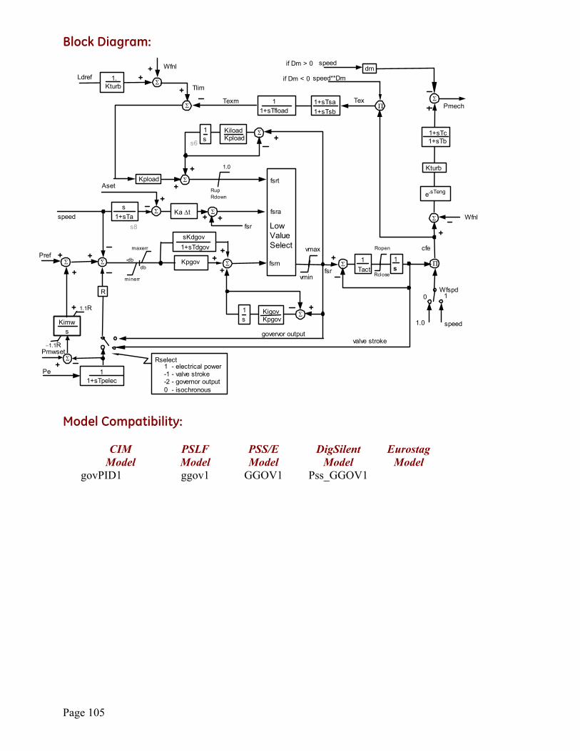
Page 105
Block Diagram:
Kpgov
sKdgov1+sTdgov
Kpload
11+sTfload
govervor outputvalve stroke
speed**Dmif Dm < 0Ldref
db-db
maxerr
minerr
1+sTsa1+sTsb
Π
speed1.0
Rclose
vmax
vminfsr
LowValueSelect
fsrt
fsra
fsrn+
++
1. Kturb
Wfnl
++
+
+
+
1.0
RupRdown
cfe
Tex
Tlim
Texm
1Tact
1s
Ropen
+
speedKa ∆t
s1+sTa
Aset
s8+ +
+
fsr
R
+
s6
+KigovKpgov
KiloadKpload +
Wfspd0 1
Wfnl
ΣPmech
1+sTc1+sTb
Kturb
e-sTeng
dmspeedif Dm > 0
+
11+sTpelec
Pe
Kimws
Pmwset
+
+ 1.1R
−1.1R
Pref +
+
1 - electrical power-1 - valve stroke-2 - governor output0 - isochronous
Rselect
1s
1s
Π
Σ
Σ
Σ
Σ Σ
Σ
Σ Σ
Σ
Σ
Σ Σ
Σ
Model Compatibility:
CIM PSLF PSS/E DigSilent Eurostag Model Model Model Model Model govPID1 ggov1 GGOV1 Pss_GGOV1
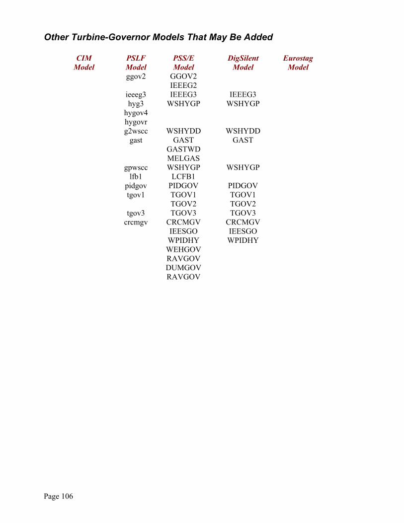
Page 106
Other Turbine-Governor Models That May Be Added CIM PSLF PSS/E DigSilent Eurostag Model Model Model Model Model ggov2 GGOV2 IEEEG2 ieeeg3 IEEEG3 IEEEG3 hyg3 WSHYGP WSHYGP hygov4 hygovr g2wscc WSHYDD WSHYDD gast GAST GAST GASTWD MELGAS gpwscc WSHYGP WSHYGP lfb1 LCFB1 pidgov PIDGOV PIDGOV tgov1 TGOV1 TGOV1 TGOV2 TGOV2 tgov3 TGOV3 TGOV3 crcmgv CRCMGV CRCMGV IEESGO IEESGO WPIDHY WPIDHY WEHGOV RAVGOV DUMGOV RAVGOV
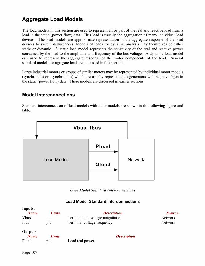
Page 107
Aggregate Load Models The load models in this section are used to represent all or part of the real and reactive load from a load in the static (power flow) data. This load is usually the aggregation of many individual load devices. The load models are approximate representation of the aggregate response of the load devices to system disturbances. Models of loads for dynamic analysis may themselves be either static or dynamic. A static load model represents the sensitivity of the real and reactive power consumed by the load to the amplitude and frequency of the bus voltage. A dynamic load model can used to represent the aggregate response of the motor components of the load. Several standard models for agregate load are discussed in this section. Large industrial motors or groups of similar motors may be represented by individual motor models (synchronous or asynchronous) which are usually represented as generators with negative Pgen in the static (power flow) data. These models are discussed in earlier sections
Model Interconnections Standard interconnection of load models with other models are shown in the following figure and table:
Pload
Vbus, fbus
Load Model NetworkQload
Load Model Standard Interconnections
Load Model Standard Interconnections Inputs:
Name Units Description Source Vbus p.u. Terminal bus voltage magnitude Network fbus p.u. Terminal voltage frequency Network Outputs:
Name Units Description Pload p.u. Load real power
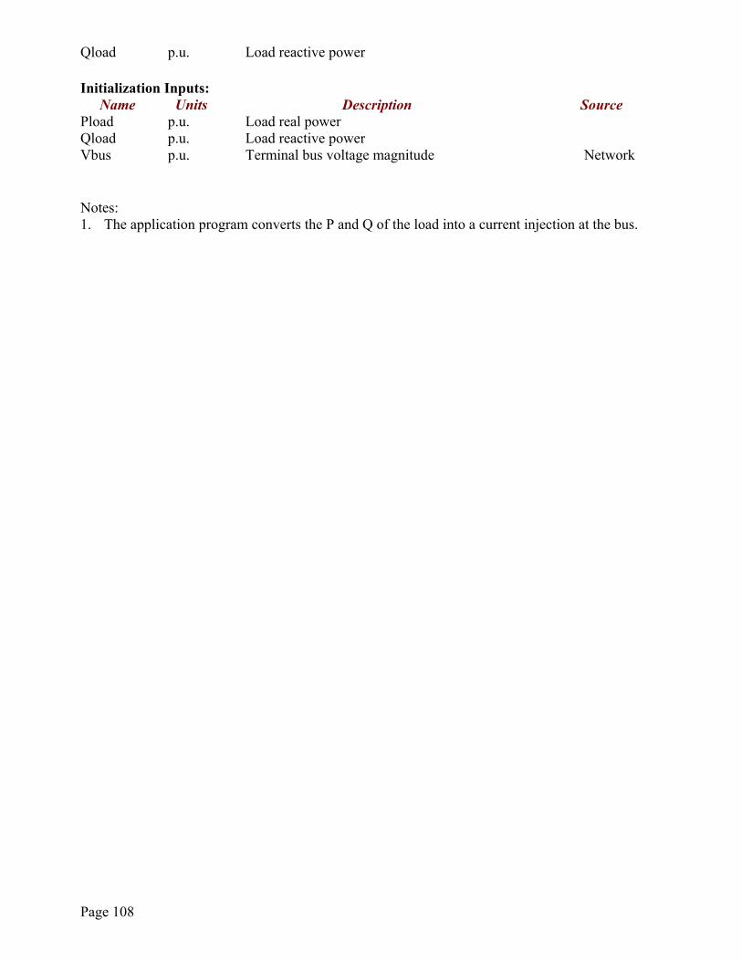
Page 108
Qload p.u. Load reactive power Initialization Inputs:
Name Units Description Source Pload p.u. Load real power Qload p.u. Load reactive power Vbus p.u. Terminal bus voltage magnitude Network Notes: 1. The application program converts the P and Q of the load into a current injection at the bus.
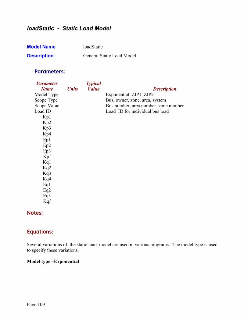
Page 109
loadStatic - Static Load Model Model Name loadStatic
Description General Static Load Model
Parameters:
Parameter Typical Name Units Value Description Model Type Exponential, ZIP1, ZIP2 Scope Type Bus, owner, zone, area, system Scope Value Bus number, area number, zone number Load ID Load ID for individual bus load Kp1 Kp2 Kp3 Kp4 Ep1 Ep2 Ep3 Kpf Kq1 Kq2 Kq3 Kq4 Eq1 Eq2 Eq3 Kqf Notes: Equations: Several variations of the static load model are used in various programs. The model type is used to specify these variations. Model type –Exponential
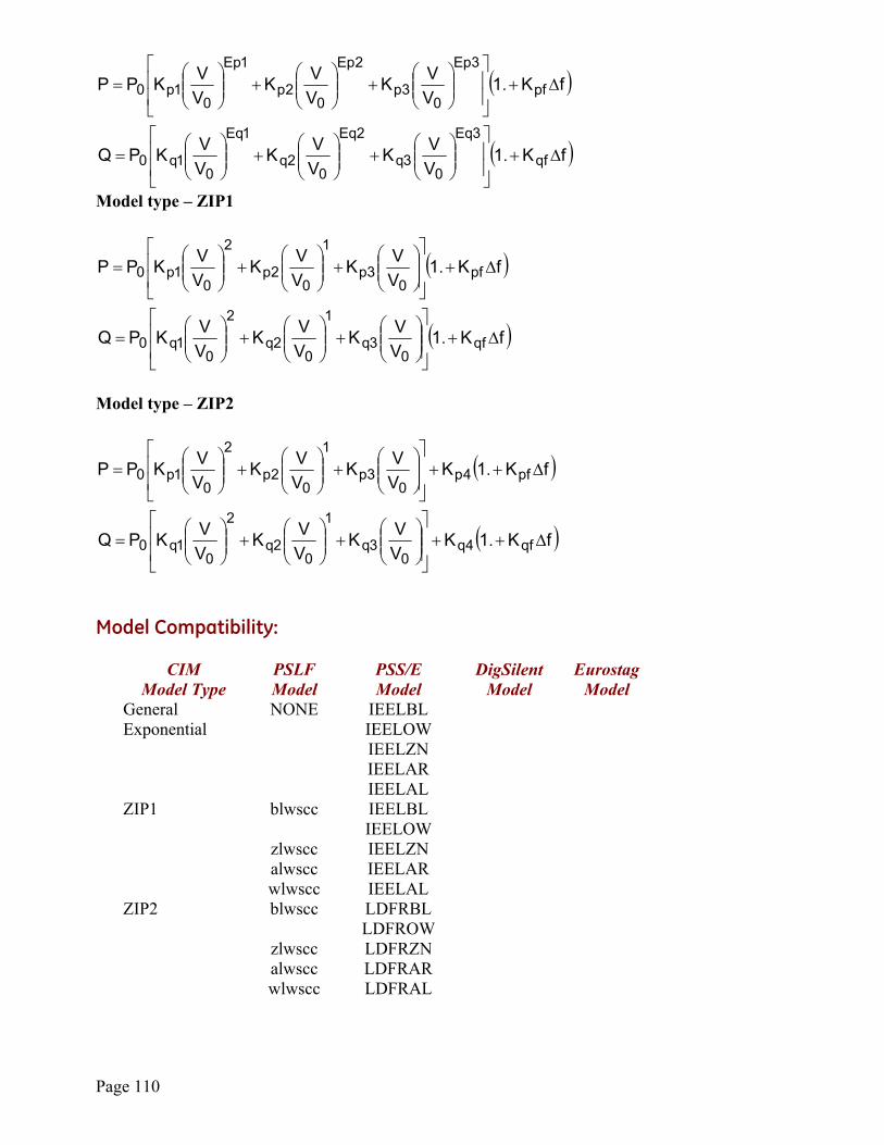
Page 110
( )
( )fK1VVK
VVK
VVKPQ
fK1VVK
VVK
VVKPP
qf
3Eq
03q
2Eq
02q
1Eq
01q0
pf
3Ep
03p
2Ep
02p
1Ep
01p0
∆+
+
+
=
∆+
+
+
=
.
.
Model type – ZIP1
( )
( )fK1VVK
VVK
VVKPQ
fK1VVK
VVK
VVKPP
qf0
3q
1
02q
2
01q0
pf0
3p
1
02p
2
01p0
∆+
+
+
=
∆+
+
+
=
.
.
Model type – ZIP2
( )
( )fK1KVVK
VVK
VVKPQ
fK1KVVK
VVK
VVKPP
qf4q0
3q
1
02q
2
01q0
pf4p0
3p
1
02p
2
01p0
∆++
+
+
=
∆++
+
+
=
.
.
Model Compatibility:
CIM PSLF PSS/E DigSilent Eurostag Model Type Model Model Model Model General
Exponential NONE IEELBL
IEELOW IEELZN IEELAR IEELAL
ZIP1 blwscc
zlwscc alwscc wlwscc
IEELBL IEELOW IEELZN IEELAR IEELAL
ZIP2 blwscc
zlwscc alwscc wlwscc
LDFRBL LDFROW LDFRZN LDFRAR LDFRAL
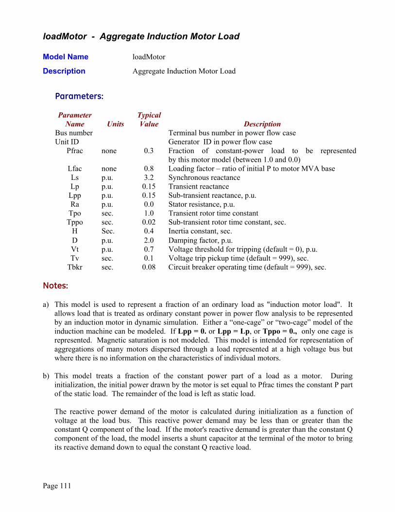
Page 111
loadMotor - Aggregate Induction Motor Load Model Name loadMotor
Description Aggregate Induction Motor Load
Parameters:
Parameter Typical Name Units Value Description Bus number Terminal bus number in power flow case Unit ID Generator ID in power flow case Pfrac none 0.3 Fraction of constant-power load to be represented
by this motor model (between 1.0 and 0.0) Lfac none 0.8 Loading factor – ratio of initial P to motor MVA base Ls p.u. 3.2 Synchronous reactance Lp p.u. 0.15 Transient reactance Lpp p.u. 0.15 Sub-transient reactance, p.u. Ra p.u. 0.0 Stator resistance, p.u. Tpo sec. 1.0 Transient rotor time constant Tppo sec. 0.02 Sub-transient rotor time constant, sec. H Sec. 0.4 Inertia constant, sec. D p.u. 2.0 Damping factor, p.u. Vt p.u. 0.7 Voltage threshold for tripping (default = 0), p.u. Tv sec. 0.1 Voltage trip pickup time (default = 999), sec. Tbkr sec. 0.08 Circuit breaker operating time (default = 999), sec. Notes: a) This model is used to represent a fraction of an ordinary load as "induction motor load". It
allows load that is treated as ordinary constant power in power flow analysis to be represented by an induction motor in dynamic simulation. Either a “one-cage” or “two-cage” model of the induction machine can be modeled. If Lpp = 0. or Lpp = Lp, or Tppo = 0., only one cage is represented. Magnetic saturation is not modeled. This model is intended for representation of aggregations of many motors dispersed through a load represented at a high voltage bus but where there is no information on the characteristics of individual motors.
b) This model treats a fraction of the constant power part of a load as a motor. During
initialization, the initial power drawn by the motor is set equal to Pfrac times the constant P part of the static load. The remainder of the load is left as static load. The reactive power demand of the motor is calculated during initialization as a function of voltage at the load bus. This reactive power demand may be less than or greater than the constant Q component of the load. If the motor's reactive demand is greater than the constant Q component of the load, the model inserts a shunt capacitor at the terminal of the motor to bring its reactive demand down to equal the constant Q reactive load.
Page 112
. c) If a motor model and a static load model are both present for a load, the motor Pfrac is
assumed to be subtracted from the power flow constant P load before the static load model is applied. The remainder of the load, if any, is then represented by the static load model.
d) The rotor time constant Tpo and inertia time constant H must be non-zero. e) Ls, Lp, Lpp must all be specified. f) D has the dimensions delta P/ delta speed. The initial value of Pmech or the value coming from
an separate mechanical load model, if used, is multiplied by speed raised to the power D to determine the effective mechanical load seen by the motor.
g) The parameters Vt and Tv define under-voltage tripping logic. A timer is started if the terminal
voltage falls below Vt per unit and continues to run until voltage rises above Vt. If voltage has not risen above Vt when the timer reaches Tv the motor is tripped immediately.
h) Per unit parameters are on the motor MVA base. The MVA base is calculated during
initialization as the initial motor P in MW divided by the loading factor (Lfac) parameter Block Diagram:
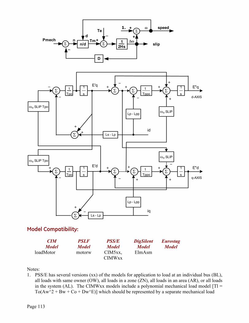
Page 113
Lp - Lpp
d-AXIS
id
E'q
Ls - Lp
E"q1Tppo s
Σ1
s
11Tpo
ωo SLIPωo SLIP Tpo
Lp - Lpp
q-AXIS
iq
E'd
Ls - Lp
E"d1Tppo s
1
s
11Tpo
ωo SLIPωo SLIP Tpo
12Hs
∆ω
D
Tespeed
Pmech
1. +
+
Σ+
_
_ω
n/dn Tm
d
Σ
Σ
Σ
Σ
Σ
Σ
ΣΣΣΣ
Σ
slip
Model Compatibility:
CIM PSLF PSS/E DigSilent Eurostag Model Model Model Model Model loadMotor motorw CIM5xx,
CIMWxx ElmAsm
Notes: 1. PSS/E has several versions (xx) of the models for application to load at an individual bus (BL),
all loads with same owner (OW), all loads in a zone (ZN), all loads in an area (AR), or all loads in the system (AL). The CIMWxx models include a polynomial mechanical load model [Tl = To(Aw^2 + Bw + Co + Dw^E)] which should be represented by a separate mechanical load
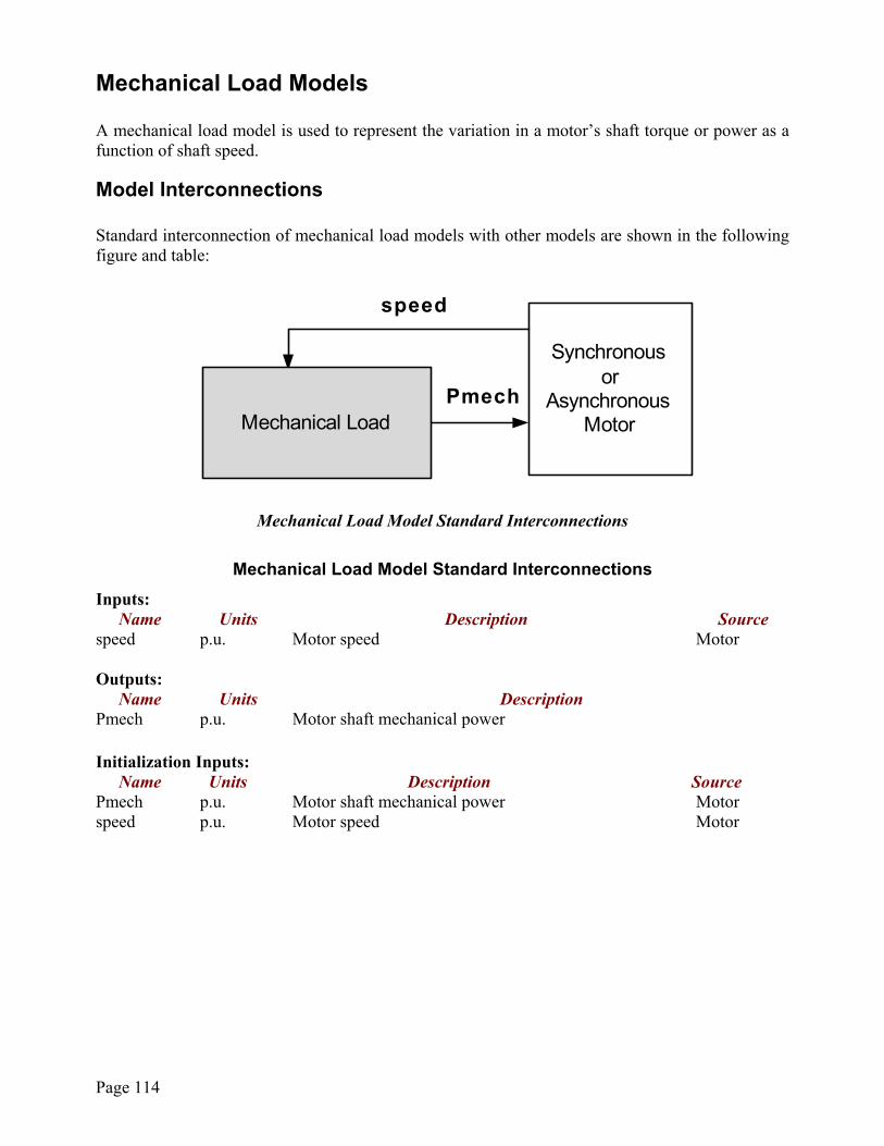
Page 114
Mechanical Load Models A mechanical load model is used to represent the variation in a motor’s shaft torque or power as a function of shaft speed.
Model Interconnections Standard interconnection of mechanical load models with other models are shown in the following figure and table:
Synchronous or
AsynchronousMotor
PmechMechanical Load
speed
Mechanical Load Model Standard Interconnections
Mechanical Load Model Standard Interconnections Inputs:
Name Units Description Source speed p.u. Motor speed Motor Outputs:
Name Units Description Pmech p.u. Motor shaft mechanical power Initialization Inputs:
Name Units Description Source Pmech p.u. Motor shaft mechanical power Motor speed p.u. Motor speed Motor
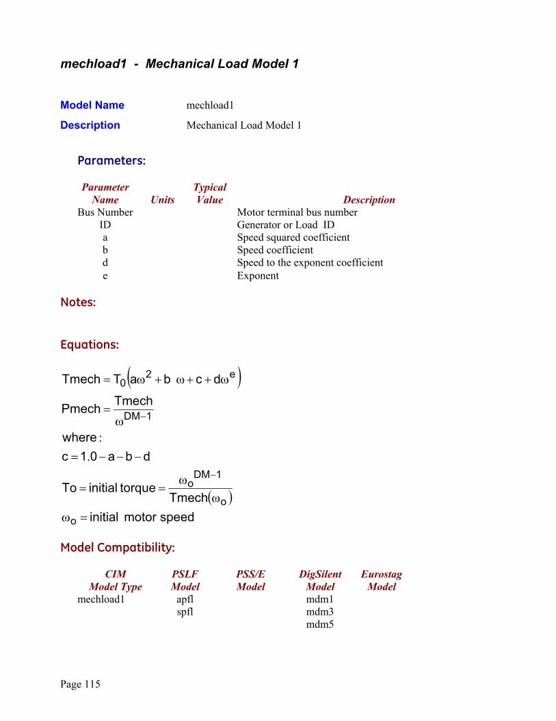
Page 115
mechload1 - Mechanical Load Model 1 Model Name mechload1
Description Mechanical Load Model 1
Parameters:
Parameter Typical Name Units Value Description Bus Number Motor terminal bus number ID Generator or Load ID a Speed squared coefficient b Speed coefficient d Speed to the exponent coefficient e Exponent Notes: Equations:
( )
( )speedmotor initial
TmechtorqueinitialTo
dba01cwhere
TmechPmech
dcbaTTmech
o
o
1DMo
1DM
e20
=ωω
ω==
−−−=
ω=
ω++ω+ω=
−
−
.:
Model Compatibility:
CIM PSLF PSS/E DigSilent Eurostag Model Type Model Model Model Model mechload1 apfl
spfl mdm1
mdm3 mdm5