Common Core Georgia Performance Standards CCGPS Mathematics

Common Core Georgia

Performance Standards CCGPS

Standards

CCGPS Pre‐Calculus

Mathematics

Georgia Department of Education

Georgia Department of Education Dr. John D. Barge, State School Superintendent

January 6, 2012 • of 18 All Rights Reserved

CCGPS Pre‐Calculus The high school standards specify the mathematics that all students should study in order to be college and career ready. Additional mathematics that students should learn in fourth credit courses or advanced courses such as calculus, advanced statistics, or discrete mathematics is indicated by (+). All standards without a (+) symbol should be in the common mathematics curriculum for all college and career ready students. Standards with a (+) symbol may also appear in courses intended for all students. The high school standards are listed in conceptual categories including Number and Quantity, Algebra, Functions, Modeling, Geometry, and Statistics and Probability. Conceptual categories portray a coherent view of high school mathematics; a student’s work with functions, for example, crosses a number of traditional course boundaries, potentially up through and including calculus. Modeling is best interpreted not as a collection of isolated topics but in relation to other standards. Making mathematical models is a Standard for Mathematical Practice, and specific modeling standards appear throughout the high school standards indicated by a star symbol (★).




Mathematics | Standards for Mathematical Practice Mathematical Practices are listed with each grade’s mathematical content standards to reflect the need to connect the mathematical practices to mathematical content in instruction. The Standards for Mathematical Practice describe varieties of expertise that mathematics educators at all levels should seek to develop in their students. These practices rest on important “processes and proficiencies” with longstanding importance in mathematics education. The first of these are the NCTM process standards of problem solving, reasoning and proof, communication, representation, and connections. The second are the strands of mathematical proficiency specified in the National Research Council’s report Adding It Up: adaptive reasoning, strategic competence, conceptual understanding (comprehension of mathematical concepts, operations and relations), procedural fluency (skill in carrying out procedures flexibly, accurately, efficiently and appropriately), and productive disposition (habitual inclination to see mathematics as sensible, useful, and worthwhile, coupled with a belief in diligence and one’s own efficacy). 1 Make sense of problems and persevere in solving them. High school students start to examine problems by explaining to themselves the meaning of a problem and looking for entry points to its solution. They analyze givens, constraints, relationships, and goals. They make conjectures about the form and meaning of the solution and plan a solution pathway rather than simply jumping into a solution attempt. They consider analogous problems, and try special cases and simpler forms of the original problem in order to gain insight into its solution. They monitor and evaluate their progress and change course if necessary. Older students might, depending on the context of the problem, transform algebraic expressions or change the viewing window on their graphing calculator to get the information they need. By high school, students can explain correspondences between equations, verbal descriptions, tables, and graphs or draw diagrams of important features and relationships, graph data, and search for regularity or trends. They check their answers to problems using different methods and continually ask themselves, “Does this make sense?” They can understand the approaches of others to solving complex problems and identify correspondences between different approaches. 2 Reason abstractly and quantitatively. High school students seek to make sense of quantities and their relationships in problem situations. They abstract a given situation and represent it symbolically, manipulate the representing symbols, and pause as needed during the manipulation process in order to probe into the referents for the symbols involved. Students use quantitative reasoning to create coherent representations of the problem at hand; consider the units involved; attend to the meaning of quantities, not just how to compute them; and know and flexibly use different properties of operations and objects. 3 Construct viable arguments and critique the reasoning of others. High school students understand and use stated assumptions, definitions, and previously established results in constructing arguments. They make conjectures and build a logical progression of statements to explore the truth of their conjectures. They are able to analyze situations by breaking them into cases, and can recognize and use counterexamples. They justify their conclusions, communicate them to others, and respond to the arguments of others. They reason inductively about data, making plausible arguments that take into account the context from which the data arose. High school students are also able to compare the effectiveness of two plausible arguments, distinguish correct logic or reasoning from that which is flawed, and—if there is a flaw in an argument—explain what it is. High school students learn to determine domains to which an argument applies, listen or read the arguments of others, decide whether they make sense, and ask useful questions to clarify or improve the arguments.




4 Model with mathematics. High school students can apply the mathematics they know to solve problems arising in everyday life, society, and the workplace. By high school, a student might use geometry to solve a design problem or use a function to describe how one quantity of interest depends on another. High school students making assumptions and approximations to simplify a complicated situation, realizing that these may need revision later. They are able to identify important quantities in a practical situation and map their relationships using such tools as diagrams, two‐way tables, graphs, flowcharts and formulas. They can analyze those relationships mathematically to draw conclusions. They routinely interpret their mathematical results in the context of the situation and reflect on whether the results make sense, possibly improving the model if it has not served its purpose. 5 Use appropriate tools strategically. High school students consider the available tools when solving a mathematical problem. These tools might include pencil and paper, concrete models, a ruler, a protractor, a calculator, a spreadsheet, a computer algebra system, a statistical package, or dynamic geometry software. High school students should be sufficiently familiar with tools appropriate for their grade or course to make sound decisions about when each of these tools might be helpful, recognizing both the insight to be gained and their limitations. For example, high school students analyze graphs of functions and solutions generated using a graphing calculator. They detect possible errors by strategically using estimation and other mathematical knowledge. When making mathematical models, they know that technology can enable them to visualize the results of varying assumptions, explore consequences, and compare predictions with data. They are able to identify relevant external mathematical resources, such as digital content located on a website, and use them to pose or solve problems. They are able to use technological tools to explore and deepen their understanding of concepts. 6 Attend to precision. High school students try to communicate precisely to others by using clear definitions in discussion with others and in their own reasoning. They state the meaning of the symbols they choose, specifying units of measure, and labeling axes to clarify the correspondence with quantities in a problem. They calculate accurately and efficiently, express numerical answers with a degree of precision appropriate for the problem context. By the time they reach high school they have learned to examine claims and make explicit use of definitions. 7 Look for and make use of structure. By high school, students look closely to discern a pattern or structure. In the expression x2 + 9x + 14, older students can see the 14 as 2 × 7 and the 9 as 2 + 7. They recognize the significance of an existing line in a geometric figure and can use the strategy of drawing an auxiliary line for solving problems. They also can step back for an overview and shift perspective. They can see complicated things, such as some algebraic expressions, as single objects or as being composed of several objects. For example, they can see 5 – 3(x – y)2 as 5 minus a positive number times a square and use that to realize that its value cannot be more than 5 for any real numbers x and y. High school students use these patterns to create equivalent expressions, factor and solve equations, and compose functions, and transform figures. 8 Look for and express regularity in repeated reasoning. High school students notice if calculations are repeated, and look both for general methods and for shortcuts. Noticing the regularity in the way terms cancel when expanding (x – 1)(x + 1), (x – 1)(x2 + x + 1), and (x – 1)(x3 + x2 + x + 1) might lead them to the general formula for the sum of a geometric series. As they work to solve a problem, derive formulas or make generalizations, high school students maintain oversight of the process, while attending to the details. They continually evaluate the reasonableness of their intermediate results.




Connecting the Standards for Mathematical Practice to the Standards for Mathematical Content The Standards for Mathematical Practice describe ways in which developing student practitioners of the discipline of mathematics increasingly ought to engage with the subject matter as they grow in mathematical maturity and expertise throughout the elementary, middle and high school years. Designers of curricula, assessments, and professional development should all attend to the need to connect the mathematical practices to mathematical content in mathematics instruction. The Standards for Mathematical Content are a balanced combination of procedure and understanding. Expectations that begin with the word “understand” are often especially good opportunities to connect the practices to the content. Students who lack understanding of a topic may rely on procedures too heavily. Without a flexible base from which to work, they may be less likely to consider analogous problems, represent problems coherently, justify conclusions, apply the mathematics to practical situations, use technology mindfully to work with the mathematics, explain the mathematics accurately to other students, step back for an overview, or deviate from a known procedure to find a shortcut. In short, a lack of understanding effectively prevents a student from engaging in the mathematical practices. In this respect, those content standards which set an expectation of understanding are potential “points of intersection” between the Standards for Mathematical Content and the Standards for Mathematical Practice. These points of intersection are intended to be weighted toward central and generative concepts in the school mathematics curriculum that most merit the time, resources, innovative energies, and focus necessary to qualitatively improve the curriculum, instruction, assessment, professional development, and student achievement in mathematics.




Mathematics | High School—Number and Quantity Numbers and Number Systems. During the years from kindergarten to eighth grade, students must repeatedly extend their conception of number. At first, “number” means “counting number”: 1, 2, 3... Soon after that, 0 is used to represent “none” and the whole numbers are formed by the counting numbers together with zero. The next extension is fractions. At first, fractions are barely numbers and tied strongly to pictorial representations. Yet by the time students understand division of fractions, they have a strong concept of fractions as numbers and have connected them, via their decimal representations, with the base‐ten system used to represent the whole numbers. During middle school, fractions are augmented by negative fractions to form the rational numbers. In Grade 8, students extend this system once more, augmenting the rational numbers with the irrational numbers to form the real numbers. In high school, students will be exposed to yet another extension of number, when the real numbers are augmented by the imaginary numbers to form the complex numbers. With each extension of number, the meanings of addition, subtraction, multiplication, and division are extended. In each new number system—integers, rational numbers, real numbers, and complex numbers—the four operations stay the same in two important ways: They have the commutative, associative, and distributive properties and their new meanings are consistent with their previous meanings. Extending the properties of whole‐number exponents leads to new and productive notation. For example, properties of whole‐number exponents suggest that (51/3)3 should be 5(1/3)3 = 51 = 5 and that 51/3 should be the cube root of 5. Calculators, spreadsheets, and computer algebra systems can provide ways for students to become better acquainted with these new number systems and their notation. They can be used to generate data for numerical experiments, to help understand the workings of matrix, vector, and complex number algebra, and to experiment with non‐integer exponents. Quantities. In real world problems, the answers are usually not numbers but quantities: numbers with units, which involves measurement. In their work in measurement up through Grade 8, students primarily measure commonly used attributes such as length, area, and volume. In high school, students encounter a wider variety of units in modeling, e.g., acceleration, currency conversions, derived quantities such as person‐hours and heating degree days, social science rates such as per‐capita income, and rates in everyday life such as points scored per game or batting averages. They also encounter novel situations in which they themselves must conceive the attributes of interest. For example, to find a good measure of overall highway safety, they might propose measures such as fatalities per year, fatalities per year per driver, or fatalities per vehicle‐mile traveled. Such a conceptual process is sometimes called quantification. Quantification is important for science, as when surface area suddenly “stands out” as an important variable in evaporation. Quantification is also important for companies, which must conceptualize relevant attributes and create or choose suitable measures for them. The Complex Number System N.CN Perform arithmetic operations with complex numbers. MCC9‐12.N.CN.3 (+) Find the conjugate of a complex number; use conjugates to find moduli and quotients of complex numbers. Represent complex numbers and their operations on the complex plane. MCC9‐12.N.CN.4 (+) Represent complex numbers on the complex plane in rectangular and polar form (including real and imaginary numbers), and explain why the rectangular and polar forms of a given complex number represent the same number. MCC9‐12.N.CN.5 (+) Represent addition, subtraction, multiplication, and conjugation of complex numbers geometrically on the complex plane; use properties of this representation for computation. For example, (‐1 + √3i)3 = 8 because (‐1 + √3i) has modulus 2 and argument 120°.




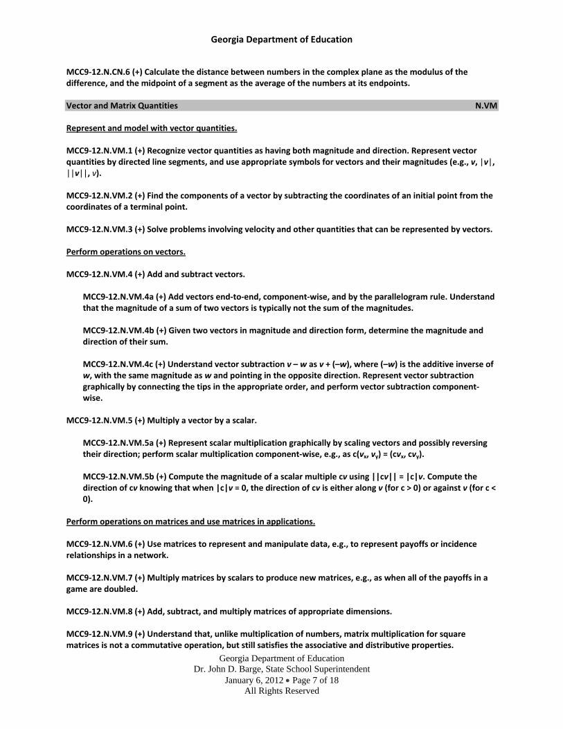
MCC9‐12.N.CN.6 (+) Calculate the distance between numbers in the complex plane as the modulus of the difference, and the midpoint of a segment as the average of the numbers at its endpoints. Vector and Matrix Quantities N.VM Represent and model with vector quantities. MCC9‐12.N.VM.1 (+) Recognize vector quantities as having both magnitude and direction. Represent vector quantities by directed line segments, and use appropriate symbols for vectors and their magnitudes (e.g., v, |v|, ||v||, v). MCC9‐12.N.VM.2 (+) Find the components of a vector by subtracting the coordinates of an initial point from the coordinates of a terminal point. MCC9‐12.N.VM.3 (+) Solve problems involving velocity and other quantities that can be represented by vectors. Perform operations on vectors. MCC9‐12.N.VM.4 (+) Add and subtract vectors.

MCC9‐12.N.VM.4a (+) Add vectors end‐to‐end, component‐wise, and by the parallelogram rule. Understand that the magnitude of a sum of two vectors is typically not the sum of the magnitudes. MCC9‐12.N.VM.4b (+) Given two vectors in magnitude and direction form, determine the magnitude and direction of their sum. MCC9‐12.N.VM.4c (+) Understand vector subtraction v – w as v + (–w), where (–w) is the additive inverse of w, with the same magnitude as w and pointing in the opposite direction. Represent vector subtraction graphically by connecting the tips in the appropriate order, and perform vector subtraction component‐wise.

MCC9‐12.N.VM.5 (+) Multiply a vector by a scalar.

MCC9‐12.N.VM.5a (+) Represent scalar multiplication graphically by scaling vectors and possibly reversing their direction; perform scalar multiplication component‐wise, e.g., as c(vx, vy) = (cvx, cvy). MCC9‐12.N.VM.5b (+) Compute the magnitude of a scalar multiple cv using ||cv|| = |c|v. Compute the direction of cv knowing that when |c|v = 0, the direction of cv is either along v (for c > 0) or against v (for c < 0).

Perform operations on matrices and use matrices in applications. MCC9‐12.N.VM.6 (+) Use matrices to represent and manipulate data, e.g., to represent payoffs or incidence relationships in a network. MCC9‐12.N.VM.7 (+) Multiply matrices by scalars to produce new matrices, e.g., as when all of the payoffs in a game are doubled. MCC9‐12.N.VM.8 (+) Add, subtract, and multiply matrices of appropriate dimensions. MCC9‐12.N.VM.9 (+) Understand that, unlike multiplication of numbers, matrix multiplication for square matrices is not a commutative operation, but still satisfies the associative and distributive properties.




MCC9‐12.N.VM.10 (+) Understand that the zero and identity matrices play a role in matrix addition and multiplication similar to the role of 0 and 1 in the real numbers. The determinant of a square matrix is nonzero if and only if the matrix has a multiplicative inverse. MCC9‐12.N.VM.11 (+) Multiply a vector (regarded as a matrix with one column) by a matrix of suitable dimensions to produce another vector. Work with matrices as transformations of vectors. MCC9‐12.N.VM.12 (+) Work with 2 X 2 matrices as transformations of the plane, and interpret the absolute value of the determinant in terms of area.




Mathematics | High School—Algebra Expressions. An expression is a record of a computation with numbers, symbols that represent numbers, arithmetic operations, exponentiation, and, at more advanced levels, the operation of evaluating a function. Conventions about the use of parentheses and the order of operations assure that each expression is unambiguous. Creating an expression that describes a computation involving a general quantity requires the ability to express the computation in general terms, abstracting from specific instances. Reading an expression with comprehension involves analysis of its underlying structure. This may suggest a different but equivalent way of writing the expression that exhibits some different aspect of its meaning. For example, p + 0.05p can be interpreted as the addition of a 5% tax to a price p. Rewriting p + 0.05p as 1.05p shows that adding a tax is the same as multiplying the price by a constant factor. Algebraic manipulations are governed by the properties of operations and exponents, and the conventions of algebraic notation. At times, an expression is the result of applying operations to simpler expressions. For example, p + 0.05p is the sum of the simpler expressions p and 0.05p. Viewing an expression as the result of operation on simpler expressions can sometimes clarify its underlying structure. A spreadsheet or a computer algebra system (CAS) can be used to experiment with algebraic expressions, perform complicated algebraic manipulations, and understand how algebraic manipulations behave. Equations and inequalities. An equation is a statement of equality between two expressions, often viewed as a question asking for which values of the variables the expressions on either side are in fact equal. These values are the solutions to the equation. An identity, in contrast, is true for all values of the variables; identities are often developed by rewriting an expression in an equivalent form. The solutions of an equation in one variable form a set of numbers; the solutions of an equation in two variables form a set of ordered pairs of numbers, which can be plotted in the coordinate plane. Two or more equations and/or inequalities form a system. A solution for such a system must satisfy every equation and inequality in the system. An equation can often be solved by successively deducing from it one or more simpler equations. For example, one can add the same constant to both sides without changing the solutions, but squaring both sides might lead to extraneous solutions. Strategic competence in solving includes looking ahead for productive manipulations and anticipating the nature and number of solutions. Some equations have no solutions in a given number system, but have a solution in a larger system. For example, the solution of x + 1 = 0 is an integer, not a whole number; the solution of 2x + 1 = 0 is a rational number, not an integer; the solutions of x2 – 2 = 0 are real numbers, not rational numbers; and the solutions of x2 + 2 = 0 are complex numbers, not real numbers. The same solution techniques used to solve equations can be used to rearrange formulas. For example, the formula for the area of a trapezoid, A = ((b1+b2)/2)h, can be solved for h using the same deductive process. Inequalities can be solved by reasoning about the properties of inequality. Many, but not all, of the properties of equality continue to hold for inequalities and can be useful in solving them. Connections to Functions and Modeling. Expressions can define functions, and equivalent expressions define the same function. Asking when two functions have the same value for the same input leads to an equation; graphing the two functions allows for finding approximate solutions of the equation. Converting a verbal description to an equation, inequality, or system of these is an essential skill in modeling. Reasoning with Equations and Inequalities A.REI Solve systems of equations MCC9‐12.A.REI.8 (+) Represent a system of linear equations as a single matrix equation in a vector variable.




MCC9‐12.A.REI.9 (+) Find the inverse of a matrix if it exists and use it to solve systems of linear equations (using technology for matrices of dimension 3 × 3 or greater).




Mathematics | High School—Functions Functions describe situations where one quantity determines another. For example, the return on $10,000 invested at an annualized percentage rate of 4.25% is a function of the length of time the money is invested. Because we continually make theories about dependencies between quantities in nature and society, functions are important tools in the construction of mathematical models. In school mathematics, functions usually have numerical inputs and outputs and are often defined by an algebraic expression. For example, the time in hours it takes for a car to drive 100 miles is a function of the car’s speed in miles per hour, v; the rule T(v) = 100/v expresses this relationship algebraically and defines a function whose name is T. The set of inputs to a function is called its domain. We often infer the domain to be all inputs for which the expression defining a function has a value, or for which the function makes sense in a given context. A function can be described in various ways, such as by a graph (e.g., the trace of a seismograph); by a verbal rule, as in, “I’ll give you a state, you give me the capital city;” by an algebraic expression like f(x) = a + bx; or by a recursive rule. The graph of a function is often a useful way of visualizing the relationship of the function models, and manipulating a mathematical expression for a function can throw light on the function’s properties. Functions presented as expressions can model many important phenomena. Two important families of functions characterized by laws of growth are linear functions, which grow at a constant rate, and exponential functions, which grow at a constant percent rate. Linear functions with a constant term of zero describe proportional relationships. A graphing utility or a computer algebra system can be used to experiment with properties of these functions and their graphs and to build computational models of functions, including recursively defined functions. Connections to Expressions, Equations, Modeling, and Coordinates. Determining an output value for a particular input involves evaluating an expression; finding inputs that yield a given output involves solving an equation. Questions about when two functions have the same value for the same input lead to equations, whose solutions can be visualized from the intersection of their graphs. Because functions describe relationships between quantities, they are frequently used in modeling. Sometimes functions are defined by a recursive process, which can be displayed effectively using a spreadsheet or other technology. Building Functions F‐BF Build new functions from existing functions MCC9‐12.F.BF.4 Find inverse functions.

MCC9‐12.F.BF.4d (+) Produce an invertible function from a non‐invertible function by restricting the domain.

Trigonometric Functions F‐TF Extend the domain of trigonometric functions using the unit circle MCC9‐12.F.TF.3 (+) Use special triangles to determine geometrically the values of sine, cosine, tangent for π/3, π/4 and π/6, and use the unit circle to express the values of sine, cosine, and tangent for π ‐ x, π + x, and 2π ‐ x in terms of their values for x, where x is any real number. MCC9‐12.F.TF.4 (+) Use the unit circle to explain symmetry (odd and even) and periodicity of trigonometric functions.




Model periodic phenomena with trigonometric functions MCC9‐12.F.TF.6 (+) Understand that restricting a trigonometric function to a domain on which it is always increasing or always decreasing allows its inverse to be constructed. MCC9‐12.F.TF.7 (+) Use inverse functions to solve trigonometric equations that arise in modeling contexts; evaluate the solutions using technology, and interpret them in terms of the context.★ Prove and apply trigonometric identities

MCC9‐12.F.TF.9 (+) Prove the addition and subtraction formulas for sine, cosine, and tangent and use them to solve problems.




Mathematics | High School—Modeling Modeling links classroom mathematics and statistics to everyday life, work, and decision‐making. Modeling is the process of choosing and using appropriate mathematics and statistics to analyze empirical situations, to understand them better, and to improve decisions. Quantities and their relationships in physical, economic, public policy, social, and everyday situations can be modeled using mathematical and statistical methods. When making mathematical models, technology is valuable for varying assumptions, exploring consequences, and comparing predictions with data. A model can be very simple, such as writing total cost as a product of unit price and number bought, or using a geometric shape to describe a physical object like a coin. Even such simple models involve making choices. It is up to us whether to model a coin as a three‐dimensional cylinder, or whether a two‐dimensional disk works well enough for our purposes. Other situations—modeling a delivery route, a production schedule, or a comparison of loan amortizations—need more elaborate models that use other tools from the mathematical sciences. Real‐world situations are not organized and labeled for analysis; formulating tractable models, representing such models, and analyzing them is appropriately a creative process. Like every such process, this depends on acquired expertise as well as creativity. Some examples of such situations might include:

• Estimating how much water and food is needed for emergency relief in a devastated city of 3 million people, and how it might be distributed. • Planning a table tennis tournament for 7 players at a club with 4 tables, where each player plays against each other player. • Designing the layout of the stalls in a school fair so as to raise as much money as possible. • Analyzing stopping distance for a car. • Modeling savings account balance, bacterial colony growth, or investment growth. • Engaging in critical path analysis, e.g., applied to turnaround of an aircraft at an airport. • Analyzing risk in situations such as extreme sports, pandemics, and terrorism. • Relating population statistics to individual predictions.

In situations like these, the models devised depend on a number of factors: How precise an answer do we want or need? What aspects of the situation do we most need to understand, control, or optimize? What resources of time and tools do we have? The range of models that we can create and analyze is also constrained by the limitations of our mathematical, statistical, and technical skills, and our ability to recognize significant variables and relationships among them. Diagrams of various kinds, spreadsheets and other technology, and algebra are powerful tools for understanding and solving problems drawn from different types of real‐world situations. One of the insights provided by mathematical modeling is that essentially the same mathematical or statistical structure can sometimes model seemingly different situations. Models can also shed light on the mathematical structures themselves, for example, as when a model of bacterial growth makes more vivid the explosive growth of the exponential function. The basic modeling cycle is summarized in the diagram. It involves (1) identifying variables in the situation and selecting those that represent essential features, (2) formulating a model by creating and selecting geometric, graphical, tabular, algebraic, or statistical representations that describe relationships between the variables, (3) analyzing and performing operations on these relationships to draw conclusions, (4) interpreting the results of the mathematics in terms of the original situation, (5) validating the conclusions by comparing them with the situation, and then either improving the model or, if it is acceptable, (6) reporting on the conclusions and the reasoning behind them. Choices, assumptions, and approximations are present throughout this cycle.




In descriptive modeling, a model simply describes the phenomena or summarizes them in a compact form. Graphs of observations are a familiar descriptive model— for example, graphs of global temperature and atmospheric CO2 over time. Analytic modeling seeks to explain data on the basis of deeper theoretical ideas, albeit with parameters that are empirically based; for example, exponential growth of bacterial colonies (until cut‐off mechanisms such as pollution or starvation intervene) follows from a constant reproduction rate. Functions are an important tool for analyzing such problems. Graphing utilities, spreadsheets, computer algebra systems, and dynamic geometry software are powerful tools that can be used to model purely mathematical phenomena (e.g., the behavior of polynomials) as well as physical phenomena. Modeling Standards Modeling is best interpreted not as a collection of isolated topics but rather in relation to other standards. Making mathematical models is a Standard for Mathematical Practice, and specific modeling standards appear throughout the high school standards indicated by a star symbol (★).




Mathematics | High School—Geometry An understanding of the attributes and relationships of geometric objects can be applied in diverse contexts—interpreting a schematic drawing, estimating the amount of wood needed to frame a sloping roof, rendering computer graphics, or designing a sewing pattern for the most efficient use of material. Although there are many types of geometry, school mathematics is devoted primarily to plane Euclidean geometry, studied both synthetically (without coordinates) and analytically (with coordinates). Euclidean geometry is characterized most importantly by the Parallel Postulate, that through a point not on a given line there is exactly one parallel line. (Spherical geometry, in contrast, has no parallel lines.) During high school, students begin to formalize their geometry experiences from elementary and middle school, using more precise definitions and developing careful proofs. Later in college some students develop Euclidean and other geometries carefully from a small set of axioms. The concepts of congruence, similarity, and symmetry can be understood from the perspective of geometric transformation. Fundamental are the rigid motions: translations, rotations, reflections, and combinations of these, all of which are here assumed to preserve distance and angles (and therefore shapes generally). Reflections and rotations each explain a particular type of symmetry, and the symmetries of an object offer insight into its attributes—as when the reflective symmetry of an isosceles triangle assures that its base angles are congruent. In the approach taken here, two geometric figures are defined to be congruent if there is a sequence of rigid motions that carries one onto the other. This is the principle of superposition. For triangles, congruence means the equality of all corresponding pairs of sides and all corresponding pairs of angles. During the middle grades, through experiences drawing triangles from given conditions, students notice ways to specify enough measures in a triangle to ensure that all triangles drawn with those measures are congruent. Once these triangle congruence criteria (ASA, SAS, and SSS) are established using rigid motions, they can be used to prove theorems about triangles, quadrilaterals, and other geometric figures. Similarity transformations (rigid motions followed by dilations) define similarity in the same way that rigid motions define congruence, thereby formalizing the similarity ideas of "same shape" and "scale factor" developed in the middle grades. These transformations lead to the criterion for triangle similarity that two pairs of corresponding angles are congruent. The definitions of sine, cosine, and tangent for acute angles are founded on right triangles and similarity, and, with the Pythagorean Theorem, are fundamental in many real‐world and theoretical situations. The Pythagorean Theorem is generalized to non‐right triangles by the Law of Cosines. Together, the Laws of Sines and Cosines embody the triangle congruence criteria for the cases where three pieces of information suffice to completely solve a triangle. Furthermore, these laws yield two possible solutions in the ambiguous case, illustrating that Side‐Side‐Angle is not a congruence criterion. Analytic geometry connects algebra and geometry, resulting in powerful methods of analysis and problem solving. Just as the number line associates numbers with locations in one dimension, a pair of perpendicular axes associates pairs of numbers with locations in two dimensions. This correspondence between numerical coordinates and geometric points allows methods from algebra to be applied to geometry and vice versa. The solution set of an equation becomes a geometric curve, making visualization a tool for doing and understanding algebra. Geometric shapes can be described by equations, making algebraic manipulation into a tool for geometric understanding, modeling, and proof. Geometric transformations of the graphs of equations correspond to algebraic changes in their equations. Dynamic geometry environments provide students with experimental and modeling tools that allow them to investigate geometric phenomena in much the same way as computer algebra systems allow them to experiment with algebraic phenomena. Connections to Equations. The correspondence between numerical coordinates and geometric points allows methods from algebra to be applied to geometry and vice versa. The solution set of an equation becomes a geometric curve, making visualization a tool for doing and understanding algebra. Geometric shapes can be described by equations, making algebraic manipulation into a tool for geometric understanding, modeling, and proof.




Similarity, Right Triangles, and Trigonometry G.SRT Apply trigonometry to general triangles MCC9‐12.G.SRT.9 (+) Derive the formula A = (1/2)ab sin(C) for the area of a triangle by drawing an auxiliary line from a vertex perpendicular to the opposite side. MCC9‐12.G.SRT.10 (+) Prove the Laws of Sines and Cosines and use them to solve problems. MCC9‐12.G.SRT.11 (+) Understand and apply the Law of Sines and the Law of Cosines to find unknown measurements in right and non‐right triangles (e.g., surveying problems, resultant forces). Expressing Geometric Properties with Equations G.GPE Translate between the geometric description and the equation for a conic section MCC9‐12.G.GPE.3 (+) Derive the equations of ellipses and hyperbolas given the foci, using the fact that the sum or difference of distances from the foci is constant.




Mathematics | High School—Statistics and Probability★ Decisions or predictions are often based on data—numbers in context. These decisions or predictions would be easy if the data always sent a clear message, but the message is often obscured by variability. Statistics provides tools for describing variability in data and for making informed decisions that take it into account. Data are gathered, displayed, summarized, examined, and interpreted to discover patterns and deviations from patterns. Quantitative data can be described in terms of key characteristics: measures of shape, center, and spread. The shape of a data distribution might be described as symmetric, skewed, flat, or bell shaped, and it might be summarized by a statistic measuring center (such as mean or median) and a statistic measuring spread (such as standard deviation or interquartile range). Different distributions can be compared numerically using these statistics or compared visually using plots. Knowledge of center and spread are not enough to describe a distribution. Which statistics to compare, which plots to use, and what the results of a comparison might mean, depend on the question to be investigated and the real‐life actions to be taken. Randomization has two important uses in drawing statistical conclusions. First, collecting data from a random sample of a population makes it possible to draw valid conclusions about the whole population, taking variability into account. Second, randomly assigning individuals to different treatments allows a fair comparison of the effectiveness of those treatments. A statistically significant outcome is one that is unlikely to be due to chance alone, and this can be evaluated only under the condition of randomness. The conditions under which data are collected are important in drawing conclusions from the data; in critically reviewing uses of statistics in public media and other reports, it is important to consider the study design, how the data were gathered, and the analyses employed as well as the data summaries and the conclusions drawn. Random processes can be described mathematically by using a probability model: a list or description of the possible outcomes (the sample space), each of which is assigned a probability. In situations such as flipping a coin, rolling a number cube, or drawing a card, it might be reasonable to assume various outcomes are equally likely. In a probability model, sample points represent outcomes and combine to make up events; probabilities of events can be computed by applying the Addition and Multiplication Rules. Interpreting these probabilities relies on an understanding of independence and conditional probability, which can be approached through the analysis of two‐way tables. Technology plays an important role in statistics and probability by making it possible to generate plots, regression functions, and correlation coefficients, and to simulate many possible outcomes in a short amount of time. Connections to Functions and Modeling. Functions may be used to describe data; if the data suggest a linear relationship, the relationship can be modeled with a regression line, and its strength and direction can be expressed through a correlation coefficient. Conditional Probability and the Rules of Probability S.CP Use the rules of probability to compute probabilities of compound events in a uniform probability model MCC9‐12.S.CP.8 (+) Apply the general Multiplication Rule in a uniform probability model, P(A and B) = [P(A)]x[P(B|A)] =[P(B)]x[P(A|B)], and interpret the answer in terms of the model.★ MCC9‐12.S.CP.9 (+) Use permutations and combinations to compute probabilities of compound events and solve problems.★




Using Probability to Make Decisions S.MD Calculate expected values and use them to solve problems MCC9‐12.S.MD.1 (+) Define a random variable for a quantity of interest by assigning a numerical value to each event in a sample space; graph the corresponding probability distribution using the same graphical displays as for data distributions.★ MCC9‐12.S.MD.2 (+) Calculate the expected value of a random variable; interpret it as the mean of the probability distribution.★ MCC9‐12.S.MD.3 (+) Develop a probability distribution for a random variable defined for a sample space in which theoretical probabilities can be calculated; find the expected value. For example, find the theoretical probability distribution for the number of correct answers obtained by guessing on all five questions of a multiple‐choice test where each question has four choices, and find the expected grade under various grading schemes.★ MCC9‐12.S.MD.4 (+) Develop a probability distribution for a random variable defined for a sample space in which probabilities are assigned empirically; find the expected value. For example, find a current data distribution on the number of TV sets per household in the United States, and calculate the expected number of sets per household. How many TV sets would you expect to find in 100 randomly selected households?★ Use probability to evaluate outcomes of decisions MCC9‐12.S.MD.5 (+) Weigh the possible outcomes of a decision by assigning probabilities to payoff values and finding expected values.★

MCC9‐12.S.MD.5a (+) Find the expected payoff for a game of chance. For example, find the expected winnings from a state lottery ticket or a game at a fast‐food restaurant.★ MCC9‐12.S.MD.5b (+) Evaluate and compare strategies on the basis of expected values. For example, compare a high‐deductible versus a low‐deductible automobile insurance policy using various, but reasonable, chances of having a minor or a major accident.★

MCC9‐12.S.MD.6 (+) Use probabilities to make fair decisions (e.g., drawing by lots, using a random number generator).★ MCC9‐12.S.MD.7 (+) Analyze decisions and strategies using probability concepts (e.g., product testing, medical testing, pulling a hockey goalie at the end of a game).★

Common Core Georgia Performance Standards CCGPS Mathematics

Documents

Transcript of Common Core Georgia Performance Standards CCGPS Mathematics