Commodity Price Volatility and Macroeconomic Fundamentals

A GARCH-MIDAS Approach

Sander van den Elzen 624024

Master of Finance December 2014

Supervisor: Dr. Lieven Baele

2

- 2014 -

Commodity Price Volatility and Macroeconomic Fundamentals

A GARCH-MIDAS Approach

Master Thesis Department Finance

S.L.J.M. van den Elzen

624024

Supervisor: Dr. Lieven Baele Second reader: Prof. Dr. L.D.R. Renneboog

3

Abstract In this research, I describe volatility dynamics of various exchange-traded commodities. The volatility of commodity prices has fluctuated substantially over the past decades, with an increase of volatility in the 2005 – 2008 period. Understanding the behaviour of volatility is crucial in derivative valuation, hedging decisions, asset allocation and risk management. Previous studies have focussed mainly on descriptive models that do not directly estimate the causal relationship between price volatility and its drivers. In this study, the unconditional volatility is modelled by linking the low-frequency deterministic component of volatility to macroeconomic variables. To do this, I make use of the GARCH-MIDAS model recently proposed by Engle et al. (2013). This framework is capable of modelling time-varying volatility by combining a mean reverting unit daily GARCH(1,1) process, and a MIDAS polynomial that applies to low-frequency macroeconomic data. Realized volatility is used to determine the best fit of the model, subsequently the monthly specification is chosen. The impact of the global economic cycle, monetary factors, market sentiment, speculative activity, convenience yield and the state of the Chinese economy is tested on six highly traded commodities. These being; Wheat, Soybeans, Gold, Silver, Crude Oil and Heating Oil. I find that models that include macroeconomic information help forecast volatility for longer horizons. Moreover, the effects of the global economic cycle, real interest rate, convenience yield and uncertainty on the Chinese economy seem to improve the capability of explaining the dynamics of unconditional price volatility over the last decades.

4

Table of Contents 1! Introduction+...............................................................................................................................+1!2! Literature+Review+....................................................................................................................+4!2.1! Time7Varying+Volatility+...............................................................................................................+4!2.2! Commodity+Volatility+Drivers+...................................................................................................+5!

3! Methodology+..............................................................................................................................+8!3.1! The+GARCH7MIDAS+model+...........................................................................................................+8!3.2! Models+with+Realized+Volatility+................................................................................................+9!3.3! Incorporating+Macroeconomic+Information+Directly+.....................................................+11!

4! Estimation+Results+................................................................................................................+12!4.1! Model+Selection+and+Estimation+with+Realized+Volatility+..............................................+12!4.1.1! Return!Data!and!Realized!Volatility!...............................................................................................!12!4.1.2! Empirical!Estimation!with!Realized!Variance!...........................................................................!13!

4.2! Estimation+with+Macroeconomic+Determinants+...............................................................+15!4.2.1! Macroeconomic!Drivers!of!Low!Frequency!Price!Volatility!................................................!15!4.2.2! Empirical!Estimation!with!Macroeconomic!Determinants!.................................................!21!

5! Conclusion+...............................................................................................................................+28!

++++++++References+..............................................................................................................................+30!++++++++Appendix+.................................................................................................................................+35!

5

List of Tables

Table 1: Parameter estimates for GARCH-MIDAS with Realized variance ........................... 14!Table 2: Estimation results Theta for macroeconomic determinants levels ............................ 22!Table 3: Estimation results Theta for macroeconomic determinants volatility ....................... 22! Table A.1: Summary Statistics Commodities Returns ............................................................ 35!Table A.2: Summary Statistics Monthly Macroeconomic Variables ...................................... 35!Table A.3: GARCH-MIDAS model with realized volatility ................................................... 36!Table A.4: GARCH-MIDAS model with realized volatility - Log Specification ................... 36!Table A.5: GARCH-MIDAS model with restriction θ =0 (GARCH(1,1)) ............................. 36!Table A.6: Estimates GARCH-MIDAS with Macroeconomic Determinants - Wheat ........... 37!Table A.7: Estimates GARCH-MIDAS with Macroeconomic Determinants - Soybeans ...... 38!Table A.8: Estimates GARCH-MIDAS with Macroeconomic Determinants - Gold .............. 39!Table A.9: Estimates GARCH-MIDAS with Macroeconomic Determinants - Silver ............ 40!Table A.10: Estimates GARCH-MIDAS with Macroeconomic Determinants – Crude ......... 41!Table A.11: Estimates GARCH-MIDAS with Macroeconomic Determinants - Heating ....... 42!Table A.12: Correlation Matrix Commodity Log Returns ...................................................... 43!Table A.13: Correlation Matrix Macroeconomic Variables .................................................... 44!

List of Figures

Figure A.1: Conditional Volatility and its Low-Frequency Component ................................. 45!Figure A.2: Optimal Weighting Functions .............................................................................. 46!Figure A.3: Distribution of Errors ........................................................................................... 47!Figure A.4: Monthly Macroeconomic Variables – Levels ...................................................... 48!Figure A.5: Monthly Macroeconomic Variables – Volatility .................................................. 49!

1

1 Introduction

Over the last decades, commodity markets have experienced dramatic growth in terms of volumes and variety of traded contracts. Furthermore, the number of operating exchanges and market participants has increased sharply (Borovkova & Geman, 2006). This gained interest in commodity derivative trading, reflects their use both as individual investments and as alternative asset class to the diversified portfolio (Edwards and Caglayan, 2001). Moreover, Brooks and Prokopczuk (2013) find a variety of reasons for the increase in commodity trading. Firstly, due to relatively poor performances of stocks and treasuries over the last decade, investors have sought new unexplored asset classes as a potential source of returns. Secondly, commodities mostly have low correlations with equity returns and the ability to provide a hedge against inflation, making them useful additions to long-term portfolios. Due to the liberalization of numerous markets, the hedging requirements for most corporations have increased over the years. This increased investment and hedging interest has led to a fast growth of the commodity derivatives market (Brooks & Prokopczuk, 2013). For most commodity markets, the price and inventory levels are characterized by periods of sharp increases and declines. Moreover, the level of volatility itself fluctuates over time (Pindyck, 2004). For the first years of this millennium, it seemed that volatility had settled, and prices showed a steady upward trend. However, the large commodity price swings observed over the last years, especially during the 2006-2009 period, quickly reminded the market of the commodities volatile nature. Moreover, it raised an extensive debate on the main determinants behind these unexpected fluctuations (Dönmez & Magrini, 2013). Throughout the literature on price volatility, it has been constantly noted that excessive price movements are harmful to both producers and consumers, particularly for those who are not able to cope with a new source of economic uncertainty. As a consequence, distinguishing the main determinants of price volatility becomes a key issue for policy-makers to intervene and reduce the potential negative effects in terms of welfare. Furthermore, Bernard et al. (2006) argue that commodity price fluctuations are economically important since they tend to impact the viability of production & investment decisions made by firms. Finally, understanding the behaviour of volatility is also important for investors of any kind. Volatility not only affects derivative valuation and hedging decisions, it is also crucial to consider for risk management and in determining the asset allocation of portfolios (Pindyck, 2004). Therefore, properly understanding and being able to model commodity price volatility, is important to all actors on the commodity market and to the academic literature. Questions related to the determination of prices and volatility of commodities have always fallen primarily in the field of microeconomics. The vast majority of literature related to this subject focuses on the relation between the volatility and ranges of demand-supply factors or market fundamentals. However, when in times so many

2

commodity prices move so far in the same direction, it becomes difficult to ignore the influence of macroeconomic circumstances. It seems that the rise and peak of almost all commodity prices in the period leading up to 2008, cannot be a coincidence (Frankel & Rose, 2010). Therefore, this study aims to link macroeconomic factors to commodity volatility dynamics over time. In order to do this, I examine time series of several macroeconomic variables that could have an impact on the commodity markets price volatility. More specifically the impact of global economic cycles, monetary factors, market sentiment, speculative activity, convenience yield and the state of the Chinese economy will be tested. Macroeconomic variables provide the advantage that they are relatively easy to collect and homogeneous over the different commodities. Numerous studies have examined models that strive to capture the time variation of volatility and its driving factors. An essential ingredient that is consistently documented is the clustering pattern of volatility. Diverse variants of the GARCH model have been pursued in different directions to deal with these phenomena (Asgharian et al., 2013). Various researchers have tried to examine the volatility pattern of commodities with different specifications of these models. However, the traditional models are often not capable to identify causal relations and are usually restricted to purely time series data (Karali & Power, 2009). The family of autoregressive conditional heteroscedasticity models has been around since the introduction by Engle (1982). Since then, various insights have been added to the academic knowledge. An important observation is that there are different components to volatility and that modeling these separately yields advantages. This insight allows us to link volatility directly to economic determinants. According to Brummer et al. (2013), previous literature on the analysis of volatility drivers can be sorted into three main categories; descriptive models, mathematical models and empirical models. Where the descriptive and mathematical models fail to describe an unrestricted causal relation. The empirical models face another common problem. The studies that investigate a causal relationship between price volatility and its drivers are often limited by the data frequency mismatch between returns and economic variables. This generates a trade-off between the possibility to exploit efficiently all the information provided by the high-frequency return data, and the necessity of investigating the linkages with the low-frequency macroeconomic determinants (Dönmez & Magrini, 2013). To address this problem some researchers narrow their scope to using only daily prices for the calculation of volatility, with the cost of having to focus only on the relationship with financial factors, lacking the ability to incorporate low-frequency economic variables (Hayo et al., 2012). Subsequently some researchers aggregate the higher frequency data to lower frequency by simply averaging, summing or assuming representative data points to proxy for low-frequency observations. This aggregation hinders extracting all available information rooted in high-frequency data and thus leads to information loss. This diminishes the estimation precision and generates poorer analysis. To overcome limitations induced by data frequency mismatches, I follow the GARCH-MIDAS model recently proposed by Engle,

3

Ghysels and Sohn (2013). This model combines a MIDAS (mixed data sampling) regression scheme with a GARCH (1,1) specification. The MIDAS component allows including data from different frequencies in the same model specification, therefore the high-frequency return data can be linked with lower-frequency macroeconomic data. The conditional variance is divided into long and short-term components, where the macroeconomic variables affect the deterministic long-term component. The model is a reduced form model, not directly linked to any structural model, and therefore ideal to implement different types of macroeconomic factors. The objective of this paper is to investigate the main drivers of commodity price volatility over the last decades, by using a framework that is able to take into consideration both high and low-frequency components of volatility. Hence, I will take into account information provided by daily prices and monthly/quarterly macroeconomic variables to describe commodity volatility dynamics. The main contribution of my analysis to the academic literature is that the trade-off between volatility measurement accuracy, provided by high-frequency return data, and including low-frequency macroeconomic data is drastically reduced. Therefore making it possible to intricately analyze the causal relationship between the price volatility and its determinants. Moreover, long horizon conditional volatility forecasting is improved by including macroeconomic information. In this analysis, I focus on six highly traded commodities that provide a good understanding of the characteristics regarding the whole commodity market. These commodities; Wheat, Soybeans, Gold, Silver, Crude Oil and Heating Oil, are examined over a 28 year period (01-01-1986 / 31-12-2013), that coincides with the era of the so-called ‘great moderation’. Data on the previously mentioned macroeconomic variables is collected for the same period, except for China’s economic state indicator. The main results of this paper show that modeling the commodity price volatility as the product of high and low-frequency components is more efficient than filtering it through a standard GARCH(1,1) model. Moreover the effects of the global economic cycle, real interest rate and the convenience yield seem to improve the capability of explaining the dynamics of unconditional price volatility over the last decades. The remainder of the paper is structured as follows; section 2 provides a study of relevant prior literature on volatility models and commodity volatility drivers. Section 3 introduces the methodology of the GARCH-MIDAS approach. The dataset and estimation results are presented in section 4, where subsection 4.1 focuses on estimations with realized volatility and subsection 4.2 provides the details and estimations of the macroeconomic variables. Finally, section 5 presents the conclusion and recommendations.

4

2 Literature Review

In this section, I will briefly discuss previous literature covering volatility models and commodity volatility drivers. As mentioned previously, commodity price volatility is appealing to both practitioners and academics, as a correct assessment of future volatility is crucial for portfolio asset allocation and risk management (Asgharian et al., 2013). The research on time-variation in volatility is extensive ever since its introduction; in fact volatility modeling has been one of the liveliest areas of study in financial econometrics (Prepic & Unosson, 2014). The increased trading of commodity futures, in combination with the recent price and volatility spikes, has lead to a surge in the literature on commodity volatility drivers. I will use the latest insights in both branches of literature to explain the dynamics of commodity volatility dynamics. First I will review the path from component volatility models to the recently proposed GARCH-MIDAS model. Thereafter I focus at previous work in the modeling of commodity specific volatility and volatility driver identification. Finally, I combine these insights of the previous literature to form the main hypothesis of this paper.

2.1 Time-Varying Volatility

Volatility modeling crucially depends on the finding that squared returns appear to be serially autocorrelated. More specifically, the volatility of returns appears to cluster so that large variations of prices follow another. This serial autocorrelation in squared returns has first been explored in the seminal paper on ARCH (AutoRegressive Conditional Heteroskedasticity) models by Engle (1982). This approach has solved problems arising with modeling time series econometrics where the assumption of homoscedasticity is violated. Besides capturing volatility clustering, the higher moment dependence structures can capture changes in return correlations and clustering of return outliers. To fully catch the dynamics of the conditional variance, oftentimes high orders of ARCH have to be used, resulting in many parameters. Later Bollerslev (1986) generalized the structure, providing us with the Generalized ARCH (GARCH) model. This model is based on an infinite ARCH specification and proves to be more parsimonious in cases of large persistence in volatility. Since Bollerslev’s introduction of the GARCH model, multiple symmetric and asymmetric variations of the model have been proposed, constituting the GARCH family. In 1993 Engle and Lee made an important observation for the progress of volatility modeling. In their paper on ‘the permanent and transitory component model of stock return volatility’, they noted that volatility is not just volatility as such, and state that there are different components to volatility. Moreover, they find that it is beneficial to model these individually. In 1999 Engle and Lee, introduced a GARCH model that identified a short and long run component to model stock return volatility. Thereafter many authors have proposed related two-factor volatility models. Chernov, Gallant,

5

Ghysels, and Tauchen (2003) examine quite an exhaustive set of diffusion models for the stock price dynamics and conclude that least two components are necessary to adequately capture the dynamics of volatility. Although the principle of multiple components is widely acknowledged, there exists no clear consensus on how to specify the component dynamics. Several papers suggest mechanisms of linking stock market volatility to macroeconomic factors, such as those of; Campbell and Hentschel (1992), Basak and Cuoco (1998), Campbell and Cochrane (1999) and Barberis, Huang and Santos (2001). However, these remain with structural models linked to one specific macroeconomic theory.

Engle and Rangel (2008) introduce a model where the daily equity volatility is a product of a slowly varying deterministic component and a mean-reverting unit GARCH, and call this the Spline-GARCH. Opposed to conventional GARCH models, this permits the unconditional volatility to change over time. Moreover, the exponential spline leads to non-negative parameterizations. Although this method achieves a better fit than the simple GARCH approach to link macroeconomic factors with stock market volatility, it is still suboptimal. In order to link the macroeconomic variables, daily equity data is averaged to match lower frequency economic series.

The model of Engle, Ghysels and Sohn (2013) accounts for this problem. They develop a framework that is inspired by recent work in mixed data sampling (MIDAS). Ghysels, Santa-Clara and Valkanov (2006) introduce a regression scheme, in the context of volatility, which allows the inclusion of data from different frequencies in the same model. They divide the conditional variance into long-term and short-term components as suggested by Engle and Lee (1999) and use the MIDAS approach to link macroeconomic variables to the long-term component. Hence smoothing the unconditional volatility’s monthly/quarterly MIDAS polynomial. Furthermore, it uses a mean reverting unit daily GARCH process, similar to Engle and Rangel (2008). Therefore, the model is called GARCH-MIDAS. The advantage of this model is that it allows to extract two components of volatility, one pertaining to short-term fluctuations, the other to a secular component. Hence, this allows to link daily return observations with macroeconomic variables, sampled at lower frequencies, to examine the macroeconomic impact on the price volatility directly. In the following subsection, I will look into the existing literature that aims to model the volatility of commodity markets.

2.2 Commodity Volatility Drivers

Over the last decades, commodity markets have experienced dramatic growth in terms of volumes and variety of traded contracts. This gained interest in commodity derivative trading is reflected in the recent academic literature. The large commodity price swings observed over the last years, especially during the 2006-2009 period, triggered an even higher interest in the subject. Subsequently, this also raised questions regarding what drivers were responsible for these patterns. Over the past few years, researchers and market specialists responded to these concerns, resulting in a rich body of literature

6

available. However, most of the literature is more focused on price levels rather than on price volatility. Nonetheless, an immaculate discussion requires careful distinction between drivers of price levels and drivers of price volatility (Brummer et al., 2013). Furthermore, various studies focus on the dynamics of commodity volatility, however fail to establish a causal relation between volatility and its drivers.

Brooks and Prokopczuk (2013), study the stochastic behaviour of prices and volatility for a sample of six important commodity markets, equivalent to those used in this study, and compare their properties to those of the equity market. However, lacking a framework to identify drivers of the dynamics, the main results merely reveal that it is inappropriate to treat different kinds of commodities as a single asset class. Moreover, they state that commodities can be a useful diversifier to equity returns as well as equity volatility. Additional descriptive studies are conducted by; Clapp (2009), Gilbert and Morgan (2010), Wright (2011), Anderson and Nelgen (2012), Chandrasekhar (2012) and Nissanke (2012), all stipulating possible drivers for commodity volatility. Fackler and Tian (1999), Balcombe (2009), Batten et al. (2010) and Ott (2013), use reduced –form models for empirical research on volatility drivers. These models define several market-specific and macroeconomic variables, however find only limited evidence that these factors influence the volatility process. Pindyck (2004), Pietola et al. (2010) and Power & Robinson (2013), employ cointegration analysis and find significant relationships for the short run. Moreover, Power & Robinson suggest that the determinants of volatility changed during the last commodity boom-and-bust cycle, yet find no evidence of drivers that influence the market volatility. Finally, a variety of authors use different specifications of the GARCH model. Zheng et al. (2008), apply an E-GARCH model to examine whether unexpected news affects food price volatility. Hayo et al. (2012) and Manera et al. (2013) use GARCH models to measure the impact of US monetary policy and speculation on price volatility of different commodities. Although intuitively promising, they encounter problems with exploiting all information efficiently due to data frequency mismatches. Roach (2010) and Karali and Power (2013) attempt to overcome this issue by employing the Spline-GARCH model, where the daily equity volatility is a product of a slowly varying deterministic component and a mean-reverting unit GARCH, enabling them to link price volatility to its macroeconomic determinants. Although this method achieves a better fit than the simple GARCH approach, it still exhibits some shortcomings. Firstly, the unconditional variance is modeled in a deterministic and non- parametric manner, preventing the possibility to incorporate directly macroeconomic data (Ghysels and Wang, 2011). Second, it requires a two-step procedure, which is not the most efficient solution, leading to a significant amount of information loss. Finally, they do not take into consideration the impact of lags regarding the macroeconomic drivers on price volatility (Donmez and Magrini, 2013). These problems could be prevailed by using the GARCH-MIDAS approach.

7

Donmez and Magrini (2013) make use of the GARCH-MIDAS model to analyze agricultural price volatility. They find that incorporating economic fundamentals into the estimation drastically improves the capability of explaining the dynamics of unconditional price volatility. Moreover, they rank their selected variables in order of importance, for the purpose of individuating addressable key drivers for policy makers. Therefore, their research focuses mainly on market specific determinants instead of macroeconomic variables. Furthermore, Donmez and Magrini only consider commodities of the cereal market; thus the analysis does not reflect price volatility for a representative of the full commodity market. Considering the literature reviewed above, I form the main research question for this research as follows: What macroeconomic determinants help describe the price volatility dynamics of commodity markets? I aim to capture this relation by employing a GARCH-MIDAS model that facilitates the inclusion of variables that are sampled at lower frequencies. Hence, overcoming problems concerning data frequency mismatches. Furthermore, I focus on six highly traded commodities that provide a good understanding of the characteristics from the whole commodity market. Following the recent co-movements in prices and volatility, I focus specifically on macroeconomic determinants opposed to market specifics.

8

3 Methodology

To determine the impact of macroeconomic variables on the price volatility of commodities, I will make use of the GARCH-Midas model. This model proposed by Engle, Ghysels and Sohn (2013) is suited to combine data that is sampled at different frequencies. The framework is inspired by the work of Ghysels, Santa-Clara and Valkonov (2006) who use mixed data sampling (MIDAS) in the context of volatility filtering to study the traditional risk-return trade-off. With this MIDAS approach, the macroeconomic variables are linked to the deterministic component of volatility. The name GARCH-MIDAS originates from the fact that it combines a mean reverting unit daily GARCH process, as used in Engle and Rangel (2008), with a MIDAS polynomial that allows incorporating low frequency financial and macroeconomic variables (monthly/quarterly/ bi-annual). Therefore, the model allows to extract two components of volatility; one related to shortterm fluctuations, the second to a secular component, and link volatility directly to economic activity.

3.1 The GARCH-MIDAS model

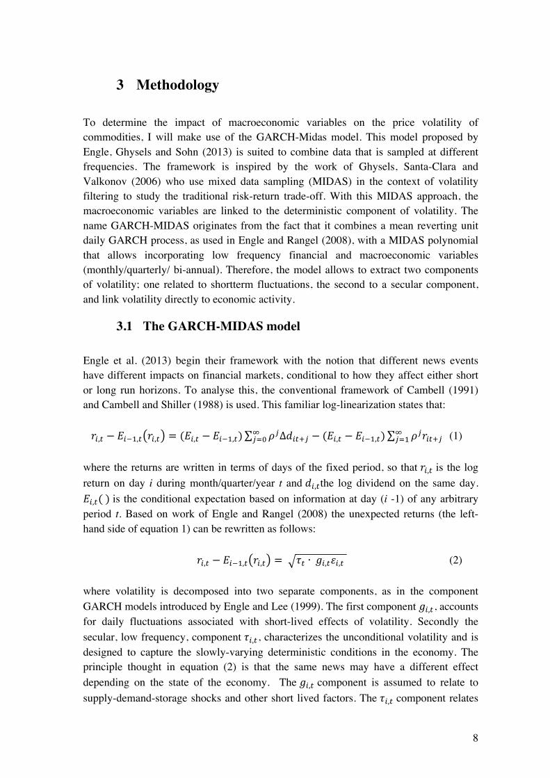
Engle et al. (2013) begin their framework with the notion that different news events have different impacts on financial markets, conditional to how they affect either short or long run horizons. To analyse this, the conventional framework of Cambell (1991) and Cambell and Shiller (1988) is used. This familiar log-linearization states that: !!!,! − !!!!,! !!,! = (!!,! − !!!!,!) !!Δ!!"!! − (!!,! − !!!!,!)!

!!! !!!!"!!!!!! (1)

where the returns are written in terms of days of the fixed period, so that !!,! is the log return on day i during month/quarter/year t and !!,!the log dividend on the same day. !!,!(!) is the conditional expectation based on information at day (i -1) of any arbitrary period t. Based on work of Engle and Rangel (2008) the unexpected returns (the left-hand side of equation 1) can be rewritten as follows: !!,! − !!!!,! !!,! = ! !! ∙ !!!,!!!,!! (2) where volatility is decomposed into two separate components, as in the component GARCH models introduced by Engle and Lee (1999). The first component !!,!, accounts for daily fluctuations associated with short-lived effects of volatility. Secondly the secular, low frequency, component !!,!, characterizes the unconditional volatility and is designed to capture the slowly-varying deterministic conditions in the economy. The principle thought in equation (2) is that the same news may have a different effect depending on the state of the economy. The !!,! component is assumed to relate to supply-demand-storage shocks and other short lived factors. The !!,! component relates

9

to macroeconomic structural factors that are assumed to explain something about the source of commodity price volatility. In this paper two cases are studied. The first case uses exclusively financial series, where the GARCH component is based on daily log returns, and the deterministic component is based on monthly realized volatility. This event is covered in subsection 3.2, in subsection 3.3 I look at an alternative specification that involve macroeconomic variables directly. The GARCH-MIDAS model with realized volatility as long run component is used as a benchmark model, where against the success of the empirical specifications with macroeconomic variables can be measured. Engle et al. (2008) consider two different options for the MIDAS filtering: one with fixed time span the other one with a rolling window. However, I will only specify the fixed span model since low-frequency macroeconomic variables are the matter of interest.

3.2 Models with Realized Volatility

Here, we start from equation (2) and consider the return for day i of any arbitrary period t (which can be a month/quarter). !! is the number of days in period t. For the model specification, the time scale of t is not important. However, empirically it will matter what frequency to select. The advantage of the model is that t will be a choice variable that will be selected as part of the model specification. For purposes of explaining the model, treat t as fixed at the monthly frequency. Assuming that !!!!,!(!!,!) is equal to !, we can rewrite equation (2) and specify the return on day i of month t as: !!,! = ! + !! ∙ !!!,!!!,!!, ∀! = 1,… ,!! (3) where !!,!!|!Φ!!!,!!~!!(0,1) with Φ!,!!! denotes the information set including the history of returns up to day (i – 1) of period t. The volatility dynamics of the !!,! component is assumed to be daily GARCH (1,1) process:

!!,! = 1− ! − ! + !! (!!!!,!!!)!

!!+ !!!!!,! (4)

where ! > 0!,!! > 0!and!! + !! < 1. The first specification of the low-frequency τ_t component for GARCH-MIDAS follows a long tradition, commenced with the works of Merton (1980) and Schwert (1989), of measuring long-run volatility by realized volatility over a monthly horizon. However, the realized volatility is not the measure of interest, instead the �_t component is specified by smoothing realized volatility with an MIDAS regression: !! = ! + ! !!(!!!!)!"!!!!

!!! (5) where !!"! is the fixed time span realized volatility at time t: !!!"! = !!,!!!!

!!! (6)

10

Also the !! is predetermined such that:

!!!! !!,! − !! = !!!!!! !!,! = !! (7)

assuming that the beginning of period expectation of the short term period is equal to its unconditional expectation such that !!!!! !!,! = 1 . Finally !!(!) is the function defining the weighting scheme for the MIDAS filter in equation (5). For this weighting function Engle et al. (2013) propose two different specifications: the Beta and the Exponential weighting lag structure. The exponential weighting function is commonly used for specifications of this kind. However, the Beta lag structure discussed in Ghysels, Sinko and Valkanov (2007) is more flexible to accommodate various lag structures. Both Engle et al. (2013) and Joyeux and Girardin (2013) show that both functions yield similar results; therefore I will only consider the Beta function:

!! !!!! = (! !)!!!!(!!! !)!!!!(! !)!!!!(!!! !)!!!!!

!!! (8)

where the weights in the equation sum up to one. Different combinations of !!!and!!! can accommodate monotonically increasing, monotonically decreasing and uni-model hump-shaped weighting schemes. Equations (3)-(6) and (8) form the GARCH-MIDAS model for time-varying conditional variance with realized variance and parameter space Θ = {!,!,!,!,!,!!,!!} . It should be emphasized that the parameter space is fixed which makes the model more parsimonious relative to other component volatility models. This feature is exploited at the stage of empirical model selection, in order to compare various GARCH-MIDAS models with different time spans t, and number of lags K. Specifically the time period t is chosen by maximizing the log-likelihood function with respect to the time span covered by RV. Subsequently the optimum number of lags K is defined by minimization of the Bayesian Information Criteria (BIC), still keeping the parameter space fixed. Finally, a log version of the !! component is proposed. This GARCH-MIDAS model replaces equation (5) by: !"#!!! = ! + ! !!(!!!!)!"!!!!

!!! (11) and is considered as it corresponds to the class, involving macroeconomic variables, introduced next.

11

3.3 Incorporating Macroeconomic Information Directly

To incorporate macroeconomic time series, the GARCH-MIDAS model has to be adjusted. The model in equation (11) involving realized variance, can conveniently be changed to insert macroeconomic variables directly, namely: !"#!!! = !! + !! !!(!!,!!!,!)!!,!!!!"!!

!!! (12) where !!,!!!!" represents the k lag of a macroeconomic variable “mv”, that we want to link to the low-frequency component of volatility. The eight macroeconomic variables of interest are defined in section 4.2.1. The subscript l indicates that we are examining the level of the macroeconomic variable (e.g. inflation, interest rate change) as is further explained in section 4.2.1. The macroeconomic series also feature volatility, i.e. inflation and interest change volatility, measured similarly as in Schwert (1989), which is further discussed in section 4.2. Incorporating these yields the next specification featuring macroeconomic volatility:

!"#!!! = !! + !! !!(!!,!!!,!)!!,!!!!"!!!!! (13)

where !!,!!!!" denotes the volatility of the explanatory series. Although the rest of the GARCH-MIDAS remains unchanged for volatility of the drivers, it should be noted that level and volatility have their own weighting schemes, hence the subscripts l and v. For equation (12) and (13) the nice features of the GARCH-MIDAS model are still in order. Firstly, making it possible to use data sampled at different frequencies. Allowing combining of high frequency financial data with macro time series available in lower frequencies, optimizing the usage of information at hand. Secondly the number of parameters stays fixed regardless of the number of lags, making it parsimonious.

12

4 Estimation Results

4.1 Model Selection and Estimation with Realized Volatility

In this section, I describe the commodities of interest for this research. Thereafter I provide an estimation of the model with realized volatility.

4.1.1 Return Data and Realized Volatility

As stated by Brooks and Prokopczuk (2013), different kinds of commodities are too heterogeneous to treat a single commodity as the entire asset class. Therefore, I carefully select six commodities that provide a good understanding about the characteristics of the whole commodity market. I focus my analysis on the following six commodities: Wheat, Soybeans, Gold, Silver, Crude Oil and Heating Oil. These are the most traded commodities within the agricultural, mineral and energy classes. Furthermore, daily future data of these series are readily available over the whole sample period, creating a reliable time series. To calculate the returns, I use daily settlement prices of the first nearby futures contract traded. For the model, the log returns are used for congruency between the classes. The specific future contracts are: Wheat No.2 soft red and Soybeans No.1 yellow, traded on the Chicago Board of Trade; Gold 100 oz., Silver 5000 oz., WTI light sweet Crude Oil and NY Harbor No.2 Heating oil, traded on the New York Mercantile Exchange, and all are quoted in US dollars. I obtain the data from Datastream for the full sample that runs from January 1st 1986 to December 31st 2013. This represents nearly 30 years of daily data (7305 observations) that coincides with the era of the so-called ‘great moderation’. Several academics; Kim & Nelson (1999), McConnell & Perez-Quiros (2000), Blanchard & Simon (2001) and Stock & Watson (2002)), find that a regime shift occurred to lower volatility of real macroeconomic activity in that time. Summary statistics from the log returns of the six commodities are presented in table A.1, and table A.12 shows the collinearity of the commodities over the sample period. The benefits of using future prices opposed to spot prices are widely acknowledged by the academic literature (Donmez & Magrini, 2013). Firstly, because they are standardized and promote accuracy; secondly they provide information on price formation to the market (Hernandez & Torero, 2010). Finally, they form a risk-transfer tool for hedgers and speculators, which is elaborated on later in this paper. Furthermore they are sampled at high frequency. Samuelson (1965) has found that price volatility increases as a futures contract approaches its delivery date. To avoid this effect throughout our time series, I follow the Method used by Gilbert (2010), and take the nearest contract until the first business day of the notional contract month, then roll over to the next trading contract month.

13

Donmez and Magrini (2013) suggest that agricultural price volatility is subjected to seasonality during a calendar year. I have taken this into account by seasonally adjusting the monthly and quarterly RV series of wheat and soybeans before fitting the MIDAS regression, as suggested by Ghysels et al. (2006). However, this did not yield a better fit, and therefore is no longer taken into account in the results presented in the following section.

4.1.2 Empirical Estimation with Realized Variance

To estimate the parameters of the GARCH-MIDAS model, I take the conventional approach to solving most GARCH-type models, namely the quasi-maximum likelihood estimation (QMLE) method. The ordinary least squares method allows the estimation of linear regressions, resulting in an approximation regarding the conditional mean of the dependent variable. However, this is limited and does not fit the purposes of many empirical studies. Therefore, maximum likelihood estimators are preferred in parameter estimations for GARCH type models, providing more consistency and efficiency. Given a certain dataset, the method of maximum likelihood allocates model parameters such that it maximizes the likelihood function. The QMLE method that I apply in this paper is a special form of the maximum likelihood functions, which allows minimization of a simplified form of the actual log-likelihood function. The model is solved in Matlab R2014A with the global optimization toolbox and multiple starting approaches to find local optimum. Parts of the code find their intuition from Sohn’s (2014) method of estimating stock market volatility. As mentioned in the methodology section, we can consider a large class of models by adjusting two features of the model. One is the frequency over which we compute RV, weighted by the MIDAS polynomial. This frequency ‘t’ can either be monthly, quarterly or biannually. As t varies the time span that !!,! is fixed changes. The other is the number of lags (K) we incorporate in each MIDAS polynomial specification for !!. More specifically I only consider full years of lags, henceforth called MIDAS lag years, such that two MIDAS lag years incorporate 8 lags (K) for quarterly specifications, and 24 lags (K) with monthly specification. Furthermore in each case two variations of the !!component with RV are possible, one for the level and one for the log specification, as described in section 3.2. The realized volatility (RV) used in equation (5) of the GARCH-MIDAS model is calculated as in equation (6) with log returns for all six commodity time series. I derive quasi-maximum likelihood estimators since these allow for possible misspecifications of the likelihood function and still achieve robust results (Donmez & Magrini, 2013). The following log-likelihood function is minimized:

!!"! = !− !! log !!"!! + (!!"!!)!

!!"!!!!!!!

!!!! (14)

14

The weights in the Beta lag structure of equation (8) are specified such that !! =1!and!!! > 1, to obtain a monotonically decreasing pattern over the lags. This is typical for volatility filters and leaves us with a simplified beta lag structure involving a single parameter. To build a proper model with macroeconomic time series later on in this paper, it is crucial to define the optimal time span t, and MIDAS lag years k, used in the MIDAS polynomial specification of the !! component. To find these, I look at the best fit of the model with realized variance. First I profile the log-likelihood function to maximize with respect to the time span covered by RV, in order to find the optimal frequency of t. My estimations indicate that the low-frequency component is best described by the monthly specification. Subsequently I look for the optimal number of lags, and thus lag years, by maximizing the Bayesian Information Criteria (BIC). Figure A.2 depicts the estimated lag weights of the GARCH-MIDAS model for all six commodities with monthly RV and three MIDAS lag years. In all cases, three MIDAS lag years fully exploits all information provided by the past values of RV since al weights converge to zero. The beta weighting structure is sufficiently flexible to describe different optimal lag patterns under three MIDAS lag years for all time series. These vary between optimal weights decaying to zero after only 8 months of lags for crude oil and up to 30 months of lags for heating oil. Consequently, I choose monthly time spans (t) and 3 MIDAS lag years (36 lags (K)) for the GARCH-MIDAS model to achieve the best representation of low-frequency volatility.

Table 1: Parameter estimates for GARCH-MIDAS with Realized variance Commodity μ α β m θ ω LLF/BIC

Wheat+ E0.000! 0.048! 0.812! 0.010! 0.177! 11.453! 17240.652!

++ !0.392! 6.579! 26.233! 14.823! 28.497! 13.315! !5.297!

Soybeans+ 0.000! 0.058! 0.930! 0.012! 0.143! 33.580! 18763.970!

0.839! 2.141! 122.817! 0.113! 2.715! 1.076! !5.765!

Gold 0.000 0.077 0.839 0.003 0.216 11.783 21393.804 + 0.032 11.125 46.225 5.811 13.163 8.434 !6.575 Silver 0.000 0.089 0.775 0.007 0.196 15.041 17681.549 0.042 10.482 26.898 12.014 6.385 3.349 !5.432 Crude 0.000 0.123 0.741 0.011 0.188 29.304 16016.906 + 0.069 3.983 6.056 8.898 3.055 2.015 !4.920 Heating 0.000 0.084 0.899 0.018 0.152 4.389 16108.293 + 0.011 12.353 109.107 2.054 1.993 0.872 !4.948 GARCH-MIDAS Realized Volatility model for the different commodities, with monthly specification and 3 MIDAS lag years. The ω in the table is ω2 as the optimal ω1 is 1 such that the optimal weights are monotonically decreasing over the lags. The numbers in the parenthesis are robust t-stats computed with HAC standard errors. LLF is the optimal log-likelihood function value and BIC is the Bayesian Information Criterion. The model is estimated for the period 1986-2013.

15

In Table 1, the parameters of the GARCH-MIDAS model with realized volatility are reported as estimated by equations (2) - (7). The parameter estimates for each commodity are shown in the first six columns. The robust t-statistics, computed with HAC standard errors, are reported underneath. Heteroscedasticity-consistent (HAC) standard errors allow the fitting of a model that contains heteroscedastic residuals. I particularly employ these errors because the assumption that the sample errors have equal variance and are uncorrelated is violated for the modelled time series. The last column shows the value of the log-likelihood function (LLF) with underneath the Bayesian Information Criteria (BIC). With exception of the ! estimator, almost all parameters are significant. More importantly for all cases ! is strongly significant and positive, indicating that the information contained in the 3 MIDAS lag years of RV help explain the low-frequency component of volatility. The ! parameter estimates suggest that higher levels of past RV lead to higher levels of !, which is as expected. An interesting feature of the GARCH-MIDAS model is that the sum of !!and!! is notable less than 1 for all commodities. While in most GARCH type models the sum is typically 1. This indicates a lower persistence in the low-frequency component of volatility, which is also found in Engle et al. (2013). Figure A.3 shows the distribution of the standard errors, which all manifest the expected curve. Figure A.1 exhibits the volatility components of the model for all commodities. It shows that the extracted ! component is smoother than the total volatility, yet still follows the path to a large extent, and captures the dynamics well. To conclude I will briefly consider the estimates of the Log!! specification, which are reported in table A.4. Overall the results are very similar to the previous specification albeit with higher theta values. Moreover, the levels of likelihood are typically lower, although the BIC criteria are very close.

4.2 Estimation with Macroeconomic Determinants

In this section, I explore the link between commodity price volatility and a broad range of macroeconomic variables. Firstly, the macro variables are identified and described. Subsequently, the model is empirically tested with the determinants incorporated directly into the GARCH-MIDAS specification.

4.2.1 Macroeconomic Drivers of Low Frequency Price Volatility

To describe the deterministic component of commodity volatility, I consider several potential drivers. I distinguish between drivers that either affect specific commodities only, or all commodities jointly. Based on the relevant literature, I selected eight candidate variables that can be classified into six main groups. These six groups will be further explained below: global economic cycle, monetary factors, market sentiment, speculative activity, convenience yield and the state of the Chinese economy. All data is obtained at a monthly frequency since the log-likelihood profile of the GARCH-MIDAS model with realized volatility suggested that the monthly frequency provided the best fit.

16

For all variables, I will look at both the level and the volatility of the macroeconomic time series in order to describe the low-frequency component of commodity volatility. With level, I refer to the absolute values of the macroeconomic variable inserted into the model, i.e. CPI inflation. With volatility, I consider the monthly variance in the macroeconomic variable, i.e. CPI inflation volatility, which is estimated similarly as in Schwert (1989). Specifically I fitted an autoregressive model with quarterly dummies to estimate monthly macroeconomic volatility: !! = !! + !!!!!! + !!!!! + !!!!! + !!!!! + !!! (14) where the parameter (!!)! constructs the monthly volatility time series for any macroeconomic variable !!. The dummies !! are added to account for seasonality in the time series, and are specified such that !!! is 1 for the months April, May and June, and zero otherwise. !!!!and !!! are defined likewise. Table A.2 presents summary statistics for each of the macroeconomic variables. To further understand the time series patterns that enter the model specification, I provide plots of the macroeconomic series in figures A.4 and A.5. Global Economic Cycle The state of the global economy is widely recognized as a crucial determinant of prices and volatility in any financial market. Prices of most financial products typically rise in times of economic upturns. Engle et al. (2013) find in their paper on stock market volatility determinants that an increase in Industrial Production growth decreases stock market volatility. This counter-cyclical pattern is also reported by Officer (1972) and Schwert (1989). Moreover, they find that the volatility in Industrial Production growth is positively related to stock market volatility, and thus stock market volatility is higher in times of economic uncertainty. For agricultural commodities Roache (2010) finds similar results, indicating that food price volatility increases when real global activity levels fall, such as in times of recession. Moreover, price volatility increases with higher variation in the global economic activity (Roache, 2010). However, Power and Robinson (2013) report that commodity price volatility increased with the commodity bull cycle of 2006 to 2008, which would indicate a positive relation. The results of Donmez and Magrini (2013) also support a positive relation, stating that a rise in global economic activity substantially increases the low-frequency component of commodity volatility. Therefore, I hypothesize that the counter cyclical pattern of volatility does not hold for commodities. To capture the impact of economic cycles, I use the growth from the Composite Leading Indicator of the global economy as a proxy for the state of the world economy. The CLI is issued monthly by the OECD and is designed to provide early signals of turning points in the business cycle. Opposed to proxies as Gross Domestic Product or Industrial Production, leading indicators provide qualitative rather than quantitative information on short-term economic movements and is capable of forecasting fluctuations of economic activity. CLI data is gathered from the OECD

17

database for the full sample, and is expected to have a positive relation with commodity volatility for both the levels and the squares. Monetary Factors I also include monetary factors from the United States into the analysis. More specifically the impact of inflation and the real interest rate are examined. The focus on the United States’ monetary policy is because commodity and commodity derivative trading mainly occurs on US exchanges. Commodities are often regarded as stores of wealth and the incentive to hold them increases with inflation (Roache, 2010). Gorton and Rouwenhorst (2006) argue that commodities are inflation hedges. Hence, inflation levels and volatility might affect commodity prices through the portfolio choices of financial investors. Karali and Power (2013) find that an increase in CPI inflation leads to an increase in price volatility, and thus levels of inflation are conjectured to have a positive relation with commodity price volatility. Roache (2010) argues that inflation volatility tends to increase low-frequency price volatility. In this research, the level of inflation is measured as the monthly growth rate of the Consumer Price Index. The time series is collected from the FRED II database, and again I expect a positive relation for both the level and volatility. As noted by Gruber and Vigfusson (2013), interest rates are an important cost to holding inventories of commodities. Low interest rates make stockpiling of commodities more attractive and larger inventories should smooth shocks to supply, indicating lower price volatility. However Frankel (2007) argues a decline in the interest rate has the effect of reducing the opportunity cost to hold inventories, increasing the commodity demand, making the market thinner and reducing the market's ability to cope with any other shock. Moreover, low interest rates are likely to cause excessive liquidity on the market, which is often blamed to exacerbate price fluctuations in the short run (Donmez and Magrini, 2013). Therefore, a negative relation between real interest rate and price volatility is expected. To account for this, I include the change in the US 3 month T-bill rate, deflated by the CPI, as a determinant. Data on the nominal short-term interest rate is taken from the FRED II database and deflated with the fisher equation. Market Sentiment Market sentiment is also considered to describe the deterministic component of commodity price volatility. As described by Gao and Suss (2013) market sentiment is a concept that reflects investor’s mood and belief, and measures the bearishness and bullishness of market participants. This market sentiment is likely to impact commodity trading in two ways; firstly in a uncertain market, producers might seek to hedge their risk against declining prices. Secondly, sentiment impacts the investor’s propensity to speculate, thus affecting liquidity. Baker and Wurgler (2006) find that sentiment can drive prices away from fundamental values and can cause shocks. Overall I find that low sentiment is likely to cause uncertainty in commodity prices and raise volatility. I hold the CBOE VIX index as a proxy for market sentiment. The VIX index, often referred to

18

as the fear index, represents the measure of markets future expected stock market volatility. Therefore, a positive relation is expected between changes in the VIX and commodity volatility. Thus, high levels and volatility of the VIX are considered to relate to high commodity price volatility. The VIX index changed its specification in 2003, the old specification continuous under the name VXO, for consistency I take the VXO specification for the entire sample. Speculative Activity Speculation on commodity markets is gaining more attention as a potential cause of the price boom and spike in the 2006 -2008 period. Economist and market analyst recently started to further investigate the role of derivate markets and speculative activity in the price formation of commodities (Donmez and Magrini, 2013). They found that informed speculation can provide liquidity, facilitate price discovery, and improve resource allocation, thereby stabilizing prices (Roache, 2010). However, if market participants are “irrational,” and trade based on emotion and herd mentality, price volatility can increase, as is described in the previous paragraph. Most prior literature has focused on linking price levels with Master’s hypothesis of driving prices away from its equilibrium (Masters, 2008). Fewer attempts are made to describe the effect of speculation on the volatility of commodity prices (Ott, 2013). To measure the effect, I make use of the Scalping index and Working-T index. The first reflects market liquidity and detects earning profits over a short period of time (Robles et al., 2009). The second is based on the distinction between market participants who trade for hedging reasons (commercial) and those who trade for profit-seeking speculative purposes (non-commercial)(Donmez and Magrini, 2010). Working (1960) defines the T-index as follows:

! =1+ ! !"#!"!!" !!!!!!!!!!"!!!!!!!!!!!!" ≥ !"1+ ! !"#!"!!" !!!!!!!!!!"!!!!!!!!!!!!" < !"

where NCS are the number of positions regarding non-commercial traders that are short. NCL is non-commercial long, CL is commercial long and CS are traders that have commercial short positions. The Working-T index measures the excess of non-commercial positions relative to hedging commercial needs; therefore it cannot be lower than one. If the index is exactly one, there is no excess speculation, and for values larger than one the excess of speculation is quantified in percentages as the index minus one. As Manera, Nicolini and Vignati (2010) report it is crucial for the calculation of the T-index how the market operators are classified. I have constructed the monthly average index using weekly data from historical commitment of trader’s reports from the Commodity Futures Trading Commission (CFTC). Where I have classified the open positions of the ‘non-reportable agents’ to the class of speculators, as suggested by Manera et al. (2010).

19

The direction of the relation between speculation and commodity price volatility is ambiguous and therefore I will state no ex-post hypothesis. Furthermore, the focus will be both on levels and squares. Potentially structural breaks will occur due to the gained interest in products on commodity derivatives over the last decade. Convenience Yield In this research, I will also consider the impact of convenience yield on the low-frequency component of commodity volatility. This convenience yield is often described as the premium associated with holding an underlying product now rather than the future contract or derivative. Pindyck (2004) finds that volatility directly influences the marginal value of storage. As the marginal value of storage (i.e. the benefit from an extra unit of inventory) is equivalent to the marginal convenience yield, it is possible to link convenience yields and the volatility of commodity prices. Moreover, Gospodinov and Ng (2011) find that convenience yields incorporate information useful for the prediction of commodity prices. As a proxy for the convenience yield, I take the spot-future spread for each of the commodities. The spot-future spread is calculated by subtracting the log spot price of the commodity from the log future price one month later. Logs of the prices are taken to provide consistency between commodities. Subsequently, the daily data is aggregated to monthly averages. The spot-future spread actually measures the inverse of the convenience yield; therefore the sign is changed before inputting the series into the model. Power and Robinson (2013) argue that convenience yields tend to be higher in times of more uncertainty in the futures market. Moreover, Frankel and Rose (2010) find that the insurance value of having an assured supply of an input is higher when the event of a disruption is more likely. Therefore, a higher spot-future spread is expected to indicate higher future volatility in commodity prices. State of the Chinese Economy Besides the economic state of the global market for producers and consumers, I specifically focus on the economic activity of China in more detail. China is an important and growing financial market that is well worth understanding, yet there is limited research covering its impact on the commodity market (Fung et al, 2003). China has emerged as one of the largest consumers markets of most primary commodities over the last years, and accounts for nearly a quarter of total commodity consumption with growth rates of nearly 20% annually in the 2000 to 2005 period (Streifel, 2006). Although the production of commodities within China is significant, overall China is a net importer of commodities and thus its impact would mainly describe the demand side of the market (Huang and Rozelle, 2006). As noted throughout the literature, the demand-supply factors are the main determinants for the price setting of commodities. The rapid growth of emerging economies, such as China, propelled the quick increase of world demands and caused commodity prices to soar before the summer of 2008 (Tang and Xiong, 2010). China’s demand for commodities is directly linked to the growth of its economy. Killian (2009) states that fluctuations in real prices of commodities are

20

historically mainly driven by demand shocks. Therefore, it is believed that changes in China’s economic cycle are positively related to commodity price volatility. To measure the state of the economy in china, I use the OECD Leading Indicator for China. This because it presents monthly data, furthermore it provides consistency between the estimators. I hypothesize that high volatility in China’s CLI will lead to high levels of price volatility. The influence of China is only perceived over the last decade and a half; therefore it will be included in the analysis for a subsample of 2000 to 2013. Relation between Macroeconomic Determinants Finally, I will examine the relations between the above-described variables. This is done to check for multicollinearity or redundancy of the various components. Although each variable is carefully chosen to describe one explicit potential determinant of the secular volatility, it is possible that overlap between variables occurs. Intuitively, concerns arise for the following variables: market sentiment, speculative activity and convenience yield. As noted earlier, when speculative traders are irrational and trade based on emotion, the effect of the speculative determinants could coincide with the sentiment index. Convenience yield could be driven by speculative activity, as non-commercial trading can drive the future prices away from (or below) the spot price and its fundamental value. Subsequently, low market sentiment could change the preferences towards holding the underlying product opposed to the contract, thus affecting convenience yield. To check to what extend the monthly time series follow the same dynamics, a correlation matrix for the macroeconomic variables is presented in table A.13. If we consider the relation between convenience yield and speculation, we find the highest correlations between convenience yield and the working T index. In the case of soybeans this goes up to 0.36, but for the other commodities this is substantially lower, with an average of 0.14. For the correlation between convenience yield and the scalping index, we find the highest value in the case of wheat, with a value of 0.24, again with substantially lower values for the other commodities. Subsequently, we find for convenience yield and the sentiment index a correlation of 0.15. Studying the relation between the sentiment index and speculation, we find considerable less correlation. With highest values of 0.05 for the Working-T index and 0.11 for the Scalping index. Moreover, I check if the two speculation proxies, the Scalping and Working T index, do not describe the same path. With an average correlation coefficient of 0.16, I infer that this is not the case. We can conclude that the highest correlations occur in the case of convenience yields, however not to troublesome extents. Finally, we find no unit root processes in the variables; hence all time series in the estimation are stationary.

21

4.2.2 Empirical Estimation with Macroeconomic Determinants

How do the above-described macroeconomic variables impact the low-frequency component of commodity price volatility? That is the question I try to answer in this section. To do this, I make use of the GARCH-MIDAS model including both macroeconomic levels and volatility time series, with τ described as in equations (12) and (13). Following previous studies (Engle et al., 2013; Asgharian et al., 2013; Conrad et al., 2012; Donmez et al., 2013), I estimate the GARCH-MIDAS model with one macroeconomic time series each time. As suggested by the estimation of the model with realized volatility, I use monthly macroeconomic series with 3 MIDAS lag years to achieve the best fit and stability. Tables A.6 - A.11 provide the parameter estimates for wheat, soybeans, gold, silver, crude and heating oil respectively. Both the estimates for the levels and volatility of the time series are presented. Again as in section 4.1.2, the t-statistics with HAC standard errors are displayed below the parameter estimates, and the last column contains the values for LLF and BIC. A nice feature of the GARCH-MIDAS model is that because of the fixed parameter space we are able to compare the different specifications. Hence, we can use the likelihood and BIC to compare which macroeconomic variable provides the best fit. For all variables, we find again that ! is in all instances very low or not significantly different for zero. Opposed to the specifications with realized volatility, m is also insignificant in most cases. However, !!and!! are in all instances strongly significant. Moreover, once controlled for macroeconomic variables, the sum is closer to 1, depicting a higher level of persistence in the price volatility. Tables 2 and 3, show the slope parameter estimates for theta of all commodities, for the levels and volatility respectively. These parameters are the most interesting for this research. Theta values explain the impact of the macroeconomic variables on the low- frequency component !. The sign and significance of each commodity – variable pair will be discussed below. I will examine the results per determinant group and subsequently look into differences between commodities.

22

Table 2: Estimation results Theta for macroeconomic determinants levels Macro+variable+ Wheat Soybeans Gold Silver Crude Heating

CLI+global+ 11.806 9.573 18.162 12.972 -0.198 -6.8610 !! 9.139 4.233 28.348 6.761 -0.231 -2.845

CLI+China+ 11.989 -3.662 12.695 9.679 -23.651 -17.772

!! 2.772 -5.254 6.692 2.612 -6.812 -3.665

CPI+Inflation+ -0.031 -0.010 2.202 2.263 -0.036 0.004

!! -0.023 -0.004 1.347 3.899 -0.013 0.002

Real+interest+rate+ -6.561 -2.465 -3.293 -10.664 -3.899 -4.231

!! -7.254 -1.736 -3.837 -11.769 -3.794 -3.306

VIX+ 2.129 1.614 0.616 0.327 0.771 -1.503

!! 6.715 5.133 6.649 2.602 1.384 -0.739

Working+T+index+ -0.001 0.001 -0.002 -0.005 0.003 -0.007

!! -0.013 0.010 -0.020 -0.044 0.002 -0.006

Scalping+Index+ 1.063 -0.002 -0.011 -0.008 0.027 -0.041

!! 0.118 -0.003 -0.052 -0.073 0.072 -0.010

Convenience+Yield+ 2.057 3.414 5.923 5.659 4.503 1.885

!! 7.543 1.782 9.172 13.346 6.289 3.153

GARCH-MIDAS model with macroeconomic level variables as specified in equation (12), for the different commodities. The model is estimated for the period 1986-2013, with monthly specification and 3 MIDAS lag years. This table shows the estimates of Theta values, the numbers below are robust t-stats computed with HAC standard errors.

Table 3: Estimation results Theta for macroeconomic determinants volatility Macro+variable+ Wheat Soybeans Gold Silver Crude Heating

CLI+global+ 206.011 179.993 209.951 185.742 139.204 263.866 !! 89.552 175.846 194.099 38.906 31.719 210.765

CLI+China+ 167.472 113.065 208.998 215.067 98.038 121.374 !! 148.209 96.373 114.087 77.155 11.930 83.324

CPI+Inflation+ 265.543 157.189 194.292 97.035 69.334 145.629

!! 14.449 147.903 160.653 50.630 69.138 123.026

Real+interest+rate+ 167.987 102.947 232.759 30.912 77.829 57.138

!! 161.911 117.457 15.004 29.833 61.319 51.773

VIX+ 1.074 2.067 1.016 0.437 0.467 0.537

!! 5.104 57.219 3.284 2.340 7.483 16.564

Working+T+index+ -0.934 -0.707 4.252 -0.324 0.021 0.406

!! -2.864 -0.835 36.808 -1.009 0.001 0.795

Scalping+Index+ 1.315 5.127 -1.190 -1.118 4.159 5.796 !! 5.534 4.178 -13.581 -2.452 1.264 12.135

Convenience+Yield+ 8.609 1.146 22.445 11.829 5.311 6.269

!! 3.729 3.085 15.255 17.019 26.109 5.211

GARCH-MIDAS model with macroeconomic volatility variables as specified in equation (13), for the different commodities. The model is estimated for the period 1986-2013, with monthly specification and 3 MIDAS lag years. This table shows the estimates of Theta values, the numbers below are robust t-stats computed with HAC standard errors.

23

Composite Leading Indicator Global Consider first the parameter estimates of !! for the CLI global variable. For most of the commodities, it shows the expected sign and is strongly significant. For wheat, soybeans, gold and silver the estimates range between 9.57 and 18.16, and thus exhibit a positive relation. This indicates that economic growth leads to higher volatility in these commodity markets. However, both energy commodities do not follow the expected sign but confer the counter-cyclical pattern suggested by Schwert (1989). Hence for crude and heating oil the volatility reduces in times of economic upturn. This could be explained by the fact that a growing economy leads to a steady demand for oil, because of an increase in investments. Since oil supply is relatively flexible, increase in constant demand can result in lower price volatility. However, this is only significant in the case of heating oil. In the case of crude oil the business cycle does not help to explain the low-frequency component of volatility. Overall the positive relation between leading indicator growth and commodity volatility dominates. Implying that a rise in the state of the global economy leads to high commodity volatility. To measure the magnitude of the impact of a change in the X variable on the low-frequency component, I follow the method proposed by Engle et al. (2013). This is done by computing the following formula: !!∗!! ! − 1 = !"#$%&!!!!! !!"!!"#"$%&'&(#&)!!"#$%&#&%'!!! In the case of wheat, the parameter estimate !!for CLI global is 11,805 with a t-statistic of 9,139. Considering that !! = 1, the beta weighting function for !! = 19.133 puts 0,423 on the first lag (!! ! = 0,423) and 0,249 on the second lag (!! ! = 0,249) of CLI global level. When computing the impact, !! !and!!! are rescaled by multiplication of 10!!!and!10!! to make the macro level variables represented in the percentage unit. The impact of a one percent increase in the composite leading indicator at the current month would increase the long-term component of next month’s wheat price volatility by !(!.!!"∗!.!"#) − 1 ≈ 0.051 or 5.1%. For the second lag, we find !(!.!!"∗!.!"#) − 1 ≈ 0.030 thus an increase in last months CLI global of 1% leads to an increase in next months low-frequency price volatility of 3,0%. For soybeans and silver a 1% increase in the current CLI leads to 3,1 and 4,0% more volatility in next month. For last months increase in CLI this is: 2,2% and 2,8% respectively. For gold a 1% increase in CLI leads to a 0,52% rise in volatility, for both the first and second lag. The cumulative effect after 6 months of 1% increase would increase the low-frequency component of volatility with more than 3%. The CLI global variable has no impact on the volatility of crude oil and a negative impact on heating oil of -6,2% for the first lag and -4,7% for the second lag. Meaning that an increase in last months CLI by 1% would reduce next months heating price volatility by 4,7%. When studying the parameter estimates of composite leading indicator growth volatility !!, we find that all the estimates are positive and highly significant. Meaning that

24

uncertainty in the economic growth leads to higher levels of deterministic commodity price volatility. If we look at the economic magnitude, we find that the impact of the volatility is about the same as the CLI growth level, ranging between 8,2% for heating oil and 0,71% for silver. Composite Leading Indicator China For the theta estimates of the composite leading indicator of china, I find values that are in line with those of the global CLI. In the case of wheat, gold and silver I find the hypothesized sign, with values between 9,68 and 12,80. This means that levels of low-frequency volatility rise in times of economic growth in China. That could be the result of commodity supply struggling to cope swiftly with the higher demand from the Chinese economy. As was with CLI global, crude and heating oil are negatively related to China’s economic growth. In this case, the parameter values are stronger with values of -17,77 & -23,65, and for both estimates significant at 1%. For CLI China, soybeans also show a negative relation. Unfortunately, I cannot explain the counter-cyclical effect that occurs with soybeans. The direct impact of China’s business cycle is smaller than that of the global economy. However, the impact is more persistent over the lags, which is caused by the weighting parameter. An increase in the leading indicator of 1% in the current month, leads to a modest increase of next month’s deterministic volatility of 0,77%. However, the 6th lag still contains enough information to predict a 0,63% increase in volatility for next month based on a 1% increase a half year ago. This persistence occurs with all commodities except for soybeans. The impact for soybeans is -0,80% for the first lag, and diminishes completely around 8 lags. For the other commodities, the impact of current months rise in CLI ranges between -1,3% for crude oil and 0,65% for gold. Concerning the uncertainty in china’s economic growth, again all the !! parameter estimates resemble those of the global economy. For all commodities, the estimates are positive and strongly significant. The impact for silver, crude oil and heating oil is again quite low and steady over the lags, with values ranging between 0,69% and 1,6%. For wheat, soybeans and gold the impact is far more direct. An increase in volatility of China’s economic growth of 1% leads to a rise in next months volatility of 7,7% for wheat. In the case of soybeans and gold this is 4,4% and 4,3% respectively. Therefore, it could be concluded that overall the commodity price volatility is more dependent on the uncertainty in china’s business cycle. Consumer Price Index Inflation Let’s take a look at the parameter estimates !! of CPI inflation for all commodities. Only for the precious metals (gold and silver) the expected sign is found. And only in the case of silver the effect is statistically significant. This means that for all commodities, except silver, CPI inflation does not influence the low-frequency volatility. For silver, the parameter value is 2.26 and hence more inflation leads to higher future price volatility. The magnitude of the impact is 0.0043, thus an increase in inflation of 1% in the current

25

month leads to an increase of 0.43% in next months volatility. This is a relatively small impact, given that a 1% increase of monthly inflation is rather high. Looking at the uncertainty of CPI inflation, we see that it is positive and significant for all commodities. With impacts ranging between 2.1% for heating oil and 0.2% for crude oil. Again although significant, the economic effect is rather small, since historically seen inflation volatility is proven to be relatively low. Real Interest Rate The second monetary policy variable, real interest rate, does show the expected values for all the parameter estimates !!. For all commodities, we find a highly significant and negative effect between real interest rate growth and price volatility. The levels range between -2,47 and -10,66, hence increases in real interest rate decreases low-frequency commodity volatility. This supports the hypothesis that a decline in interest rate reduces the opportunity cost to hold inventories, hence making the market thinner and reducing the ability to cope with shocks. The economic impact is quite high for both energy commodities, with -3,0% and -3,3% for crude and heating oil respectively. For gold and silver a 1% increase in the real interest rate at the current month, leads to a decline in volatility of -1,2% and -1,4% for the following month. For the agricultural commodities, the effect is quite divers, for wheat an increase of 1% in the interest rate leads to a decline of 5,3% and for soybeans this is only 0,83%. This seems to be the effect of differences in storability of the commodities. Uncertainty in the real interest rates also yields significant results, albeit with low impact for most commodities. For heating oil, gold, silver and soybeans the effect ranges between 0,16% and 1,2% in ascending order. The real interests rate does have quite a large impact on the price volatility of crude oil, with an increase of 1% in interest rate leading to a decline in volatility of 3,9% the following month. In the case of wheat, the effect of the real interest rate could not be adequately modelled. Although the theta estimate of 167.99 with a t-stat of 161.91 seems to have quite a significant effect, no global optimum could be found, with the result that the alpha value increased to 0,99. Therefore real interest rate uncertainty does not affect the price volatility of wheat. VIX The market sentiment indicator, VIX, is expected to describe a positive relation with commodity volatility. Thus, an increase in the volatility index leads to higher secular commodity volatility. The expected signs are found for all commodities except heating oil. Though, in the case of both energy commodities the value is not statistically significant. Implying that market sentiment does not affect the volatility of crude and heating oil. For the remaining four products, the parameter estimates are significant but far lower than for the previous variables, with values of 2.13 & 1.61 for the agricultural commodities and 0.62 & 0.33 for the precious metals. The magnitude of the impact ranges between 0,27% and 0,54% increase of volatility for a 1% increase in the VIX, and is highly persistent over the lags for the agricultural commodities. Although this

26

impact may not appear high, it must be noted that a 1% increase in the VIX is very small on monthly basis. When looking at the summary statistics in table A.2, we see that a 2.1% change is the average on monthly basis. Therefore, I conclude that precious metals, and to an even larger extend agricultural commodity volatility, is positively linked with market sentiment. More specifically when the VIX rises the commodity volatility of next month will rise as well. The parameter estimates of the volatility of the VIX !! are for all cases significant but small. The impact however is negligible with values between 0,02% and 0,04%. Working-T Index The working T index is the first of two proxies I use to analyse the effect of speculative activity on commodity volatility. Within recent literature, destabilising speculation has come up repeatedly as a possible cause of the past price and volatility spikes (Frankel and Rose, 2010). The T index measures excess of non-commercial positions relative to commercial needs and is expected to exhibit a positive relation with volatility, meaning that high values of speculative trading lead to more price volatility. However, the parameter estimates !! indicate both positive and negative relations, yet are in no instance statistically significant. The uncertainty in speculation parameter !! is significant for wheat and gold, but the impact is again negligible. Therefore, I must state that I do not find any effect of the Working-T index on the volatility of the six tested commodities for the 1986 -2013 sample. Scalping Index The scalping index is the second variable I use to proxy speculative activity. The scalping index reflects market liquidity and detects short period speculation. The parameter estimates show results similar to that of the Working-T index. The values of the estimates are low, and the signs show no consistency over the commodities. In none of the cases the estimate is statistically significant. The parameter of the variance in the scalping index !! is in all cases, except crude oil, significant. For wheat, soybeans and heating the impact is 0,02% with a 1% increase in volatility of the index. For the precious metals, the impact is -0,12% for the first lag but decays immediately after. Thus both proxies for speculative activity seem to have no effect. Therefore, I conclude that speculative activity does not influence the secular component of commodity volatility. Convenience Yield Growth in the premium associated with holding an underlying product now, rather than the future contract or derivative is expected to indicate higher future volatility in commodity prices. The parameter estimates !! for the convenience yield seem to support this assertion. For all of the commodities, the values show the expected sign and are strongly significant. The slope estimates range between 1.89 for heating oil and 5.92 for gold. The values for silver and crude oil are close to that of gold, with 5.66 and 4.50 respectively. For volatility in convenience yield, a similar result is found; again all of the values are positive and strongly significant. Moreover, gold, silver and crude oil exhibit

27

again the largest and significantly strongest effect. This supports the claim that convenience yields tend to be higher in times of more uncertainty in the futures market, and that the insurance value of having an assured supply of an input is higher when the event of a disruption is more likely. The magnitude of the impact regarding convenience yield levels range between 0.13% for heating oil and 0.80% for gold. This means that a one-unit change of the convenience yield at the current month would increase the long-term component of next month’s gold price volatility by 0.8%. For all commodities the impact is persistent through time, due to a relatively flat weighting function. The information provided in the second lag still forecasts an impact of 0.71% for gold. The impact of volatility in convenience yield is only considerable in the case of gold, with a 1,01% impact for the first lag. Distinctions Between Commodity Markets Finally I consider the differences of determinant impacts between the distinct commodities. Overall the results are quite coherent over the different markets. In all markets, speculative activity has no significant impact. If we focus at the log-likelihood values in the last column of tables A.6 – A.11, we can see which models achieve the best fit. For wheat, I find that the GARCH-MIDAS models with real interest rate and market sentiment describe the low-frequency component of volatility best. CPI inflation provides the worst fit, describing the model no better than the standard GARCH(1,1). However, the uncertainty in CPI inflation does provide a good fit. For soybeans, the best fit of the model is described by the global economic cycle and market sentiment. The volatility of the monetary factors outperforms the other specifications. In the case of gold, convenience yield describes the low-frequency component of volatility best. Moreover, real interest rate and market sentiment provide a good fit of the model. Again the monetary factor’s volatility contributes considerable to the model, as well as convenience yield uncertainty. For silver, the best fit of the model is provided by the inclusion of the global economic cycle and convenience yield. Remarkable is that only for silver the effect of inflation is significant, and enhances the results considerable. The specification for crude oil is the only one that does not recognise the global economic cycle as contributor to deterministic volatility. Moreover, market sentiment provides no information on its volatility dynamics. The best fit of the model is achieved by real interest rates and convenience yields. Heating oil is also not affected by the volatility index, however does state significant effect for the global economic cycle. Table A.5 shows the estimation results for the restricted specification of equation (12), where θ = 0 which reduces the GARCH-MIDAS model to a GARCH(1,1) model with constant unconditional variance. Comparing the LLF, I show that the GARCH-MIDAS model with any macroeconomic variable included always outperforms the GARCH(1,1).

28

5 Conclusion

In this paper, I set out to explain the dynamics of commodity price volatility. The striking price movements off all commodity markets in the 2006 - 2009 period cause the focus on this subject. The markets prices, and level of volatility, have historically always fluctuated over time, however the movements of different commodities in the same direction over last decades is remarkable. Understanding the behaviour of volatility is crucial in derivative valuation, hedging decisions, asset allocation and risk management. Hence, distinguishing the main determinants of price volatility becomes a key issue. Therefore, I aim to link macroeconomic factors to commodity volatility dynamics over time. In the previous literature, numerous studies strive to capture the time variation of volatility and its driving factors. However, many of those studies use traditional models that are often not capable to identify causal relations and are usually restricted to purely time series data. The studies that do investigate a causal relationship between price volatility and its drivers are often limited by the data frequency mismatch between returns and economic variables. Differently from those previous studies, I manage to link the information coming from the high-frequency data on daily prices directly to the macroeconomic determinants sampled at lower-frequency in one single model without information loss resulting from aggregation. To do so, I make use of the GARCH-MIDAS model of Engle et al. (2013), which is a new class component volatility model providing a unified framework to handle data in different time frequencies. The high-frequency component reflects the daily fluctuations of volatility with a mean reverting GARCH(1,1). The low-frequency component characterizes the unconditional volatility, which captures the highly persistent conditions in the economy by the MIDAS regression. Hence, I investigate the main drivers of commodity price volatility over the last decades by taking into account information provided by daily prices and monthly macroeconomic variables. The main contribution of my analysis to the academic literature is that the trade-off between volatility measurement accuracy, provided by high-frequency return data, and including low-frequency macroeconomic data is drastically reduced. This makes it possible to intricately analyze the causal relationship between the price volatility and its determinants. Moreover, long horizon conditional volatility forecasting is improved by including macroeconomic information. Practitioners can benefit from the results through the identified macroeconomic drivers, such that the volatility of commodities can be forecasted. I focus on six highly traded commodities that provide a good understanding of the characteristics regarding the whole commodity market. These commodities; Wheat, Soybeans, Gold, Silver, Crude Oil and Heating Oil are examined over the 1986 – 2013

29

sample. First, I regress the commodities on realized volatility to define the optimal time span t, and MIDAS lag years k, used in the MIDAS polynomial specification of the !! component. The estimations indicate that the low-frequency component is best described by the monthly specification with three years of lags. Subsequently, I identify several potential drivers based on relevant literature, in order to capture the effect of macroeconomic factors on commodity volatility. I selected eight candidate variables that can be classified into six main groups. For these six groups: global economic cycle, monetary factors, market sentiment, speculative activity, convenience yield and the state of the Chinese economy, both the level and volatility are modelled. Once I estimate the models using macroeconomic determinants, I observe that the global economic cycle, real interest rate and the convenience yield seem to explain a large part of the deterministic volatility. Moreover, uncertainty on the Chinese economy seems to have a considerable impact on the low-frequency component of volatility. However, there are some differences in estimation results for different commodities. Specifically, the results suggest that convenience yield is particularly important in the case of gold, silver and crude oil. Market sentiment, improves the fit of all models, except for the energy markets. The volatility in monetary factors contributes considerably to the model in all of the cases. However, I do not find any evidence that speculative activity influenced the secular component of commodity volatility over the last decades. Moreover, I show that the GARCH-MIDAS models always outperform the standard GARCH(1,1), indicating that a time-varying unconditional variance model accommodates the price volatility behavior better. A limitation of the study is that no tests have been done to investigate the presence of structural breaks in the conditional volatility. Previous literature reports that breaks might occur in coincidence with the recent large price swings. Moreover, the forecasting performance of the model including macroeconomic variables is not empirically tested against other specifications. This eliminates the possibility to quantify the added performance of the GARCH-MIDAS model against traditional models. For further research, I would thus recommend to test forecast performance with an RMSE model to appraise the contribution of the economic resources. Furthermore I would suggest modelling multiple macroeconomic variables in the same specification, to appreciate each individual contribution and recognise overlap in determinants.

30

References

Anderson, K., and Nelgen, S. (2012). Trade barrier volatility and agricultural price stabilization. World Development. 40(1): 36–48.

Asgharian, H., Hou, A. J. and, Javed, F. (2013). Importance of the macroeconomic variables for volatility prediction: A GARCH-Midas approach. Journal of Forecasting, forthcoming, ISSN: 0277-6693.

Baker, M., & Wurgler, J. (2006). Investor sentiment and the cross‐section of stock returns. The Journal of Finance, 61(4), 1645-1680.

Balcombe, K. (2009). The nature and determinants of volatility in agricultural prices: An empirical study from 1962–2008. In The evolving structure of world agricultural trade (eds Sarris A., Morrison J.): 109– 136. Rome, Italy: FAO.

Barberis, N., & Huang, M. J. Santos,(2001) Prospect Theory and Asset Pricing. Quarterly Journal of Economics, forthcoming.

Basak, S., & Cuoco, D. (1998). An equilibrium model with restricted stock market participation. Review of Financial Studies, 11(2), 309-341.

Batten, J. A., Ciner, C., & Lucey, B. M. (2010). The macroeconomic determinants of volatility in precious metals markets. Resources Policy, 35(2), 65-71.

Blanchard, O., & Simon, J. (2001). The long and large decline in US output volatility. Brookings papers on economic activity, 2001(1), 135-174.

Bollerslev, T. (1986). A conditionally heteroskedastic time series model for speculative prices and rates of return. The review of economics and statistics, 542-547.

Borovkova, S., & Geman, H. (2006). Seasonal and stochastic effects in commodity forward curves. Review of Derivatives Research, 9(2), 167-186.

Brooks, C., & Prokopczuk, M. (2013). The dynamics of commodity prices. Quantitative Finance, 13(4), 527-542.

Brümmer, B., Korn, O., Schlüßler,K., Jaghdani, T. J. and Saucedo, A. (2013). Volatility in the after crisis period–A literature review of recent empirical research. Working Paper 1, ULYSSES project, EU 7th Framework Programme, Project 312182 KBBE. 2012.1. 4-05.

Campbell, J. Y., & Shiller, R. J. (1988). The dividend-price ratio and expectations of future dividends and discount factors. Review of financial studies, 1(3), 195-228.

Campbell, J. Y. (1991). A variance decomposition for stock returns (No. w3246). National Bureau of Economic Research.

Campbell, J. Y., & Hentschel, L. (1992). No news is good news: An asymmetric model of changing volatility in stock returns. Journal of financial Economics, 31(3), 281-318.

Campbell, J. Y., & Cochrane, J. H. (2000). Explaining the poor performance of consumption‐based asset pricing models. The Journal of Finance, 55(6), 2863-2878.

Chandrasekhar, C. P. (2012). Food price levels and volatility: Sources, impact and implications. IDS Bulletin, 43 (Supplement s1): 74–83.

31

Chernov, M., Ronald Gallant, A., Ghysels, E., & Tauchen, G. (2003). Alternative models for stock price dynamics. Journal of Econometrics, 116(1), 225-257.

Clapp, J. (2009). Food price volatility and vulnerability in the global south: Considering the global economic context. Third World Quarterly, 30(6): 1183–1196.

Conrad, C., Loch, K. and Rittler, D.(2012). On the macroeconomic determinants of the long-term oil-stock correlation. University of Heidelberg, Department of Economics, Discussion Paper No. 525.

Donmez, A., & Magrini, E. (2013). Agricultural Commodity Price Volatility and Its Macroeconomic Determinants: A GARCH-MIDAS Approach (No. JRC84138). Institute for Prospective and Technological Studies, Joint Research Centre.

Edwards, F. R., & Caglayan, M. O. (2001). Hedge funds and commodity fund investments in bull and bear markets. Available at SSRN 281522.

Engle, R.F. (1982), "Autoregressive conditional heteroscedasticity with estimates of the variance of United Kingdom inflation." Econometrica: Journal of the Econometric Society 987-1007.

Engle, R. F., & Lee, G. G. (1993). A permanent and transitory component model of stock return volatility. University of California at San Diego, Economics Working Paper Series.

Engle, R. F., & Lee, G. (1999). A long-run and short-run component model of stock return volatility. Cointegration, Causality, and Forecasting: A Festschrift in Honour of Clive WJ Granger, 475-497.

Engle, R. F., & Rangel, J. G. (2008). The spline-GARCH model for low-frequency volatility and its global macroeconomic causes. Review of Financial Studies, 21(3), 1187-1222.

Engle, R.F., Ghysels, E. and Sohn, B. (2013). Stock market volatility and macroeconomic fundamentals. The Review of Economics and Statistics, 95(3): 776–797.

Fackler, P. L., & Tian, Y. (1999). Volatility models for commodity markets. Applied commodity price analysis, forecasting and market risk management, Chicago, IL.

Frankel, J. A. (2007). The effect of monetary policy on real commodity prices. In J. Campbell (ed.), Asset Prices and Monetary Policy, University of Chicago Press, Chicago, III.

Frankel, J. A., & Rose, A. K. (2010). Determinants of agricultural and mineral commodity prices.

Fung, H. G., Leung, W. K., & Xu, X. E. (2003). Information flows between the US and China commodity futures trading. Review of Quantitative Finance and Accounting, 21(3), 267-285.

Gao, L., & Süss, S. (2013). Market Sentiment in Commodity Futures Returns. Available at SSRN 1934397.

Ghysels, E., Santa-Clara, P. and Valkanov, R. (2005). There is a risk-return trade-off after all. Journal of Financial Economics 76: 509-548.

32

Ghysels, E., Santa-Clara, P. and Valkanov, R. (2006). Predicting volatility: getting the most out of return data sampled at different frequencies. Journal of Econometrics 131: 59–95.

Ghysels, E., Sinko, A., & Valkanov, R. (2007). MIDAS regressions: Further results and new directions. Econometric Reviews, 26(1), 53-90.

Ghysels, E. and Wang F. (2011). Statistical inference for volatility component models. UNC discussion paper..

Gilbert, C. L., (2010). Speculative Influences on Commodity Futures Prices 2006-2008. United Nations Conference on Trade and Development (UNCTAD) Discussion Papers No. 197.

Gilbert, C.L. and Morgan, C. W. (2010). Food price volatility. Philosophical Transactions of the Royal Society B, 365: 3023–3034. doi:10.1098/ rstb.2010.0139.

Girardin, E., & Joyeux, R. (2013). Macro fundamentals as a source of stock market volatility in China: A GARCH-MIDAS approach. Economic Modelling, 34, 59-68.

Gorton, G& Rouwenhorst, K. G. (2006) "Facts and Fantasies About Commodity Futures” Financial Analysts Journal,62 (2) 47-68.

Gospodinov, N., & Ng, S. (2013). Commodity prices, convenience yields, and inflation. The Review of Economics and Statistics, 95(1), 206-219.

Gruber, J. W., & Vigfusson, R. J. (2012). Interest rates and the volatility and correlation of commodity prices. Federal Reserve Board.

Hayo, B., Kutan, A. M., & Neuenkirch, M. (2012). Communication matters: US monetary policy and commodity price volatility. Economics Letters, 117(1), 247-249.

Hernandez, M., & Torero, M. (2010). Examining the dynamic relationship between spot and future prices of agricultural commodities (No. 988). International Food Policy Research Institute (IFPRI).

Huang, J., & Rozelle, S. (2006). The emergence of agricultural commodity markets in China. China Economic Review, 17(3), 266-280.

Karali, B., & Power, G. J. (2009). What explains high commodity price volatility? Estimating a unified model of common and commodity-specific, high-and low-frequency factors. In 2009 Annual Meeting, July 26-28, 2009, Milwaukee, Wisconsin (No. 49576). Agricultural and Applied Economics Association.

Karali B. and Power, G. J. (2013). Short- and long-run determinants of commodity price volatility. American Journal of Agricultural Economics 95(3): 724-738.

Kilian L. (2009). Not all oil price shocks are alike: Disentangling demand and supply shocks in the crude oil market. American Economic Review 99(3): 1053-69.

Kim, C. J., & Nelson, C. R. (1999). Has the US economy become more stable? A Bayesian approach based on a Markov-switching model of the business cycle. Review of Economics and Statistics, 81(4), 608-616.

McConnell, M. M., & Perez-Quiros, G. (2000). Output fluctuations in the United States: What has changed since the early 1980's?. American Economic Review, 1464-1476.

33

Masters, M. W. (2008) Testimony before the U.S. Senate Committee of Homeland Security and Government Affairs. Washington, DC, 20 May 2008.

Manera, M., Nicolini, M., & Vignati, I. (2013). Futures price volatility in commodities markets: The role of short term vs long term speculation.

Merton, R. C. (1980). On estimating the expected return on the market: An exploratory investigation. Journal of Financial Economics, 8(4), 323-361.

Nissanke, M. (2012). Commodity Market Linkages in the Global Financial Crisis: Excess Volatility and Development Impacts. Journal of Development Studies 48(6): 732–750.

Officer, R. R. (1973). The variability of the market factor of the New York Stock Exchange. Journal of Business, 434-453.

Ott, H. (2013). Extent and possible causes of intrayear agricultural commodity price volatility. Agricultural Economics. doi: 10.1111/agec.12043.

Pietola, K., Liu, X., and Robles, M. (2010). Price, inventories, and volatility in the global wheat market. International Food Policy Research Institute (IFPRI), IFPRI discussion papers 01/2010.

Pindyck, R. S. (2004). Volatility and commodity price dynamics. Journal of Futures Markets, 24(11), 1029-1047.

Power, G. J., & Robinson, J. R. (2013). Commodity futures price volatility, convenience yield and economic fundamentals. Applied Economics Letters, 20(11), 1089-1095.

Prepic, A., and Unosson, M., 2014. A Comparison of GARCH-class Models and MIDAS Regression with Applications in Volatility Prediction and Value at Risk Estimation. Working Paper, Upsalla University.

Roache, S. K. (2010). What explains the rise in food price volatility? International Monetary Fund (IMF) Working Papers 10/129. Washington DC: International Monetary Fund.

Robles, M., Torero, M. and von Braun, J. (2009). When speculation matters. International Food Policy Research Institute (IFPRI) Issue Brief 57, Washington, DC.

Samuelson, P. (1965). Proof that properly anticipated prices fluctuate randomly. Industrial Management Review 6: 41-49.

Schwert, G. W. (1989). Why does stock market volatility change over time?. The journal of finance, 44(5), 1115-1153.

Sohn, Bumjean; Ghysels, Eric; Engle, Robert, "Replication data for: Stock Market Volatility and Macroeconomic Fundamentals", http://dx.doi.org/10 .7910/DVN/27513 V1

Streifel, S. (2006). Impact of China and India on global commodity markets: focus on metals and minerals and petroleum. Development Prospects Group/World Bank, UU World Investment Report.

Stock, J. H., & Watson, M. W. (2003). Has the business cycle changed and why?. In NBER Macroeconomics Annual 2002, Volume 17 (pp. 159-230). MIT press.

Tang, K., & Xiong, W. (2010). Index investment and financialization of commodities (No. w16385). National Bureau of Economic Research.

34

Working, H. (1960). Speculation on hedging markets. Food Research Institute Studies, (02).

Wright, B. D. (2011). The economics of grain price volatility. Applied Economic Perspectives and Policy 33(1): 32–58.

Zheng, Y., Kinnucan, H. W., & Thompson, H. (2008). News and volatility of food prices. Applied Economics, 40(13), 1629-1635.

35

Appendix

Table A.1: Summary Statistics Commodities Returns

Table A.2: Summary Statistics Monthly Macroeconomic Variables Macro determinant Mean STD Skew Kurt Min Max

CLI global growth 0.00003 0.00172 -0.61759 7.44300 -0.00821 0.00622

CLI china growth 0.00001 0.00405 -0.24690 6.87820 -0.01553 0.01275

CPI inflation 0.00227 0.00263 -1.45250 14.90270 -0.01771 0.01377

Δ Real interest rate -0.00020 0.00353 -0.07443 4.68326 -0.01136 0.01538

Δ VIX 0.02107 0.23324 2.35950 14.48660 -0.45027 1.72970

Working T Wheat 1.48210 0.21229 1.50270 6.61230 1.19610 2.60180

Soybeans 1.40630 0.14900 0.38007 2.22180 1.16570 1.78280

Gold 1.23340 0.07641 0.42618 3.05080 1.09160 1.47220

Silver 1.25990 0.13007 2.20280 9.04730 1.09980 1.88800

Crude 1.18430 0.05882 0.76637 3.54240 1.07650 1.39970

Heating 1.22810 0.08717 0.78394 3.32350 1.08400 1.52210

Scalping Wheat 0.27558 0.23492 5.57480 41.16160 0.11780 2.53690

Soybeans 0.18125 0.12369 4.21640 22.93450 0.05468 1.04640

Gold 0.21293 0.08257 0.89130 3.91860 0.07214 0.52704

Silver 0.23939 0.10055 0.95308 5.16850 0.03770 0.75114

Crude 0.15428 0.03906 0.33329 2.80070 0.07516 0.28975

Heating 0.16562 0.04306 0.49980 2.89880 0.06746 0.30305

Convenience Yield Wheat 0.04331 0.11567 1.03640 5.90050 -0.30047 0.61964

Soybeans 0.02225 0.06572 -0.51250 5.81940 -0.26374 0.27295

Gold 0.00606 0.03616 0.36139 4.36110 -0.11916 0.15911

Silver 0.00302 0.06444 0.10079 4.70760 -0.22044 0.25847

Crude 0.00292 0.08580 -0.44145 5.91150 -0.39958 0.37667

Heating 0.00277 0.09228 -0.39122 4.39100 -0.30530 0.36790

Commodity+ Mean+ STD+ Skew+ Kurt+ Min+ Max+

Wheat+ 0.00008! 0.01799! E0.07131! 8.27670! E0.16001! 0.12929!

Soybeans+ 0.00012! 0.01468! E0.61468! 8.62500! E0.14083! 0.07543!

Gold+ 0.00018! 0.01027! E0.27154! 10.97950! E0.09821! 0.08887!

Silver+ 0.00016! 0.01824! E0.79235! 10.88230! E0.19518! 0.12358!

Crude+ 0.00018! 0.02433! E0.84231! 18.50360! E0.40048! 0.16410!

Heating+ 0.00018! 0.02368! E1.42860! 22.15240! E0.39094! 0.13994!

36

Table A.3: GARCH-MIDAS model with realized volatility Commodity μ α β m θ ω LLF/BIC Wheat+ E0.000! 0.048! 0.812! 0.010! 0.177! 11.453! 17240.652!

++ !0.392! 6.579! 26.233! 14.823! 28.497! 13.315! !5.297!

Soybeans+ 0.000! 0.058! 0.930! 0.012! 0.143! 33.580! 18763.970!

0.839! 2.141! 122.817! 0.113! 2.715! 1.076! !5.765!

Gold 0.000 0.077 0.839 0.003 0.216 11.783 21393.804 + 0.032 11.125 46.225 5.811 13.163 8.434 !6.575 Silver 0.000 0.089 0.775 0.007 0.196 15.041 17681.549 0.042 10.482 26.898 12.014 6.385 3.349 !5.432 Crude 0.000 0.123 0.741 0.011 0.188 29.304 16016.906 + 0.069 3.983 6.056 8.898 3.055 2.015 !4.920 Heating 0.000 0.084 0.899 0.018 0.152 4.389 16108.293 + 0.011 12.353 109.107 2.054 1.993 0.872 !4.948

Table A.4: GARCH-MIDAS model with realized volatility - Log Specification Commodity+ μ+ α+ β+ m+ θ+ ω+ LLF/BIC+

Wheat+ E0.000! 0.161! 0.839! 0.025! 10.137! 9.499! 17032.579!

++ !0.356- 15.610- 81.416- 0.015- 2.341- 6.714- !5.232-

Soybeans+ 0.000! 0.122! 0.878! 0.004! 6.527! 17.437! 18599.263!

++ 0.999- 17.591- 126.113- 0.036- 3.488- 5.495- !5.714-

Gold+ 0.000! 0.145! 0.855! 0.002! E14.354! 3.931! 21155.884!

++ 0.288- 17.860- 105.456- 0.013- !10.196- 2.267- !6.501-

Silver+ E0.000! 0.173! 0.827! 0.009! 7.566! 6.040! 17479.282!

!0.083- 14.344- 68.805- 0.059- 9.021- 4.316- !5.370-

Crude+ 0.000! 0.116! 0.884! 0.021! 6.916! 4.766! 15938.054!

++ 1.761- 2.988- 22.802- 0.399- 2.047- 3.112- !4.896-

Heating+ 0.000! 0.128! 0.872! 0.021! 6.341! 7.743! 16004.695!

++ 0.401- 20.730- 141.397- 0.154- 6.990- 3.542- !4.943-

Table A.5: GARCH-MIDAS model with restriction θ =0 (GARCH(1,1)) Commodity+ μ+ α+ β+ m+ θ+ ω+ LLF/BIC+

Wheat+ 0.000! 0.161! 0.840! 0.021! E! E! 17029.570!

++ !1.054- 15.927- 83.075- 0.072- !- !- !5.232-

Soybeans+ 0.000! 0.122! 0.878! 0.019! E! E! 18595.254!

++ 0.100- 18.066- 129.549- 0.1338- !- !- !5.714-

Gold+ 0.000! 0.120! 0.880! 0.039! E! E! 21149.453!

++ 0.196- 13.247- 96.884- 0.328- !- -- !6.499-

Silver+ 0.000! 0.142! 0.858! 0.019! E! E! 17474.923!

!0.020- 14.325- 86.511- 0.173- !- !- !5.369-

Crude+ 0.000! 0.116! 0.884! 0.022! E! E! 15935.054!

++ 1.769- 13.579- 103.620- 0.179- !- !- !4.895-

Heating+ 0.001! 0.128! 0.872! 0.023! E! E! 15999.694!

++ 2.145- 17.690- 120.600- 0.155- !- !- !4.915-

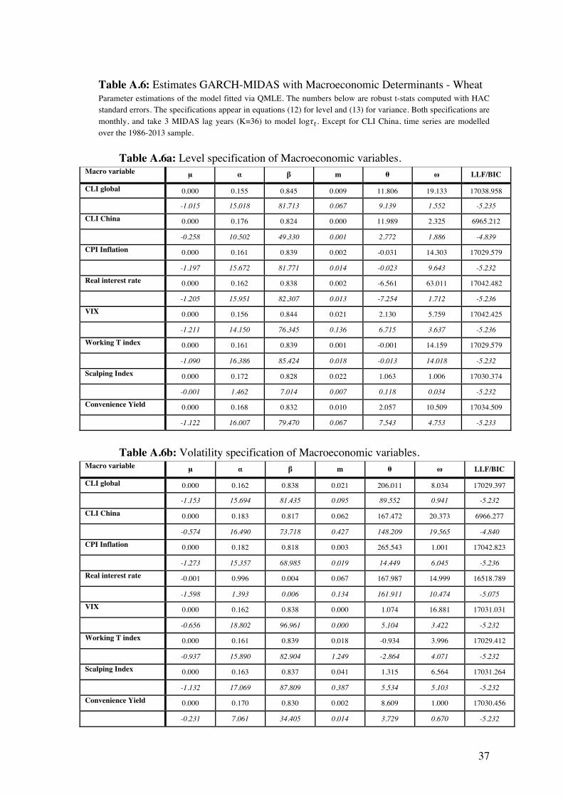
37

Table A.6: Estimates GARCH-MIDAS with Macroeconomic Determinants - Wheat Parameter estimations of the model fitted via QMLE. The numbers below are robust t-stats computed with HAC standard errors. The specifications appear in equations (12) for level and (13) for variance. Both specifications are monthly, and take 3 MIDAS lag years (K=36) to model log!!. Except for CLI China, time series are modelled over the 1986-2013 sample.

Table A.6a: Level specification of Macroeconomic variables.

Macro variable μ α β m θ ω LLF/BIC

CLI global 0.000 0.155 0.845 0.009 11.806 19.133 17038.958 -1.015 15.018 81.713 0.067 9.139 1.552 -5.235

CLI China 0.000 0.176 0.824 0.000 11.989 2.325 6965.212

-0.258 10.502 49.330 0.001 2.772 1.886 -4.839

CPI Inflation 0.000 0.161 0.839 0.002 -0.031 14.303 17029.579 -1.197 15.672 81.771 0.014 -0.023 9.643 -5.232

Real interest rate 0.000 0.162 0.838 0.002 -6.561 63.011 17042.482 -1.205 15.951 82.307 0.013 -7.254 1.712 -5.236

VIX 0.000 0.156 0.844 0.021 2.130 5.759 17042.425

-1.211 14.150 76.345 0.136 6.715 3.637 -5.236

Working T index 0.000 0.161 0.839 0.001 -0.001 14.159 17029.579

-1.090 16.386 85.424 0.018 -0.013 14.018 -5.232

Scalping Index 0.000 0.172 0.828 0.022 1.063 1.006 17030.374 -0.001 1.462 7.014 0.007 0.118 0.034 -5.232

Convenience Yield 0.000 0.168 0.832 0.010 2.057 10.509 17034.509 -1.122 16.007 79.470 0.067 7.543 4.753 -5.233

Table A.6b: Volatility specification of Macroeconomic variables.

Macro variable μ α β m θ ω LLF/BIC

CLI global 0.000 0.162 0.838 0.021 206.011 8.034 17029.397 -1.153 15.694 81.435 0.095 89.552 0.941 -5.232

CLI China 0.000 0.183 0.817 0.062 167.472 20.373 6966.277

-0.574 16.490 73.718 0.427 148.209 19.565 -4.840

CPI Inflation 0.000 0.182 0.818 0.003 265.543 1.001 17042.823

-1.273 15.357 68.985 0.019 14.449 6.045 -5.236

Real interest rate -0.001 0.996 0.004 0.067 167.987 14.999 16518.789

-1.598 1.393 0.006 0.134 161.911 10.474 -5.075

VIX 0.000 0.162 0.838 0.000 1.074 16.881 17031.031

-0.656 18.802 96.961 0.000 5.104 3.422 -5.232

Working T index 0.000 0.161 0.839 0.018 -0.934 3.996 17029.412

-0.937 15.890 82.904 1.249 -2.864 4.071 -5.232

Scalping Index 0.000 0.163 0.837 0.041 1.315 6.564 17031.264

-1.132 17.069 87.809 0.387 5.534 5.103 -5.232

Convenience Yield 0.000 0.170 0.830 0.002 8.609 1.000 17030.456

-0.231 7.061 34.405 0.014 3.729 0.670 -5.232

38

Table A.7: Estimates GARCH-MIDAS with Macroeconomic Determinants - Soybeans Parameter estimations of the model fitted via QMLE. The numbers below are robust t-stats computed with HAC standard errors. The specifications appear in equations (12) for level and (13) for variance. Both specifications are monthly, and take 3 MIDAS lag years (K=36) to model log!!. Except for CLI China, time series are modelled over the 1986-2013 sample.

Table A.7a: Level specification of Macroeconomic variables. Macro+variable+ μ+ α+ β+ m+ θ+ ω+ LLF/BIC+CLI+global+ 0.000! 0.122! 0.878! 0.001! 9.573! 13.555! 18596.701!!! 0.999! 17.228! 123.546! 0.008! 4.233! 1.512! !5.714-CLI+China+ 0.001! 0.212! 0.788! 0.075! E3.662! 8.594! 7675.067!!! 1.861! 20.547! 76.220! 0.830! !5.254! 7.601! !5.334-CPI+Inflation+ 0.000! 0.122! 0.878! 0.003! E0.010! 1.085! 18595.264!!! 0.993! 18.056! 129.548! 0.020! !0.004! 0.413! !5.714-Real+interest+rate+ 0.000! 0.123! 0.877! 0.001! E2.465! 14.317! 18594.756!!! 1.049- 17.549- 125.388- 0.004- !1.736- 14.244- !5.713-VIX+ 0.000! 0.122! 0.878! 0.018! 1.614! 6.541! 18600.383!!! 1.036- 16.989- 122.736- 0.147- 5.133- 3.183- !5.715-Working+T+index+ 0.000! 0.122! 0.878! 0.018! 0.001! 16.803! 18595.254!!! 0.906- 17.082- 122.434- 0.147- 0.010- 9.645- !5.714-Scalping+Index+ 0.000! 0.122! 0.878! 0.018! E0.002! 2.956! 18595.254!!! 1.009- 17.479- 125.338- 0.146- !0.003- 9.442- !5.714-Convenience+Yield+ 0.000! 0.122! 0.878! 0.018! 3.414! 82.588! 18595.256!!! 0.257- 19.254- 137.968- 0.147- 1.782- 15.724- !5.714-

Table A.7b: Volatility specification of Macroeconomic variables.

Macro+variable+ μ+ α+ β+ m+ θ+ ω+ LLF/BIC+

CLI+global+ 0.000! 0.123! 0.877! 0.016! 179.993! 18.307! 18595.233!!! 0.952! 16.376! 117.048! 0.119! 175.846! 14.286! !5.714-

CLI+China+ 0.001! 0.214! 0.786! 0.021! 113.065! 16.982! 7675.328!

!! 1.961! 14.022! 51.596! 0.370! 96.373! 16.334! !5.334-

CPI+Inflation+ 0.000! 0.126! 0.874! 0.041! 157.189! 2.603! 18597.452!

!! 0.986! 16.756! 116.520! 0.329! 147.903! 3.260! !5.714-

Real+interest+rate+ 0.000! 0.124! 0.876! 0.000! 102.947! 4.332! 18593.440!

!! 0.977- 16.673- 117.335- 0.004- 117.457- 6.808- !5.713-

VIX+ 0.000! 0.127! 0.873! 0.145! 2.067! 4.646! 18584.925!

!! 0.996- 16.930- 115.939- 3.398- 57.219- 25.989- !5.710-

Working+T+index+ 0.000! 0.127! 0.873! 0.210! E0.707! 15.116! 18593.226!

!! 1.010- 11.583- 79.522- 2.215- !0.835- 15.112- !5.713-

Scalping+Index+ 0.000! 0.125! 0.875! 0.002! 5.127! 1.001! 18597.951!

!! 0.520- 15.204- 106.217- 0.017- 4.178- 0.978- !5.714-

Convenience+Yield+ 0.000! 0.123! 0.877! 0.018! 1.146! 15.708! 18595.007!

!! 0.918- 16.605- 118.704- 0.157- 3.085- 14.982- !5.713-

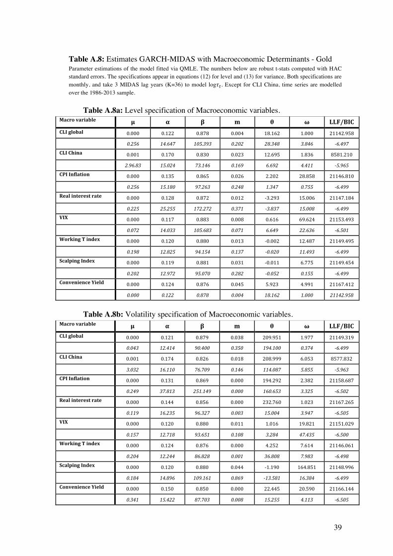
39

Table A.8: Estimates GARCH-MIDAS with Macroeconomic Determinants - Gold Parameter estimations of the model fitted via QMLE. The numbers below are robust t-stats computed with HAC standard errors. The specifications appear in equations (12) for level and (13) for variance. Both specifications are monthly, and take 3 MIDAS lag years (K=36) to model log!!. Except for CLI China, time series are modelled over the 1986-2013 sample.

Table A.8a: Level specification of Macroeconomic variables. Macro+variable+ μ+ α+ β+ m+ θ+ ω+ LLF/BIC+

CLI+global+ 0.000! 0.122! 0.878! 0.004! 18.162! 1.000! 21142.958!!! 0.256- 14.647- 105.393- 0.202- 28.348- 3.846- !6.497-

CLI+China+ 0.001! 0.170! 0.830! 0.023! 12.695! 1.836! 8581.210!

!! 2.96.83- 15.024- 73.146- 0.169- 6.692- 4.411- !5.965-

CPI+Inflation+ 0.000! 0.135! 0.865! 0.026! 2.202! 28.858! 21146.810!

!! 0.256- 15.180- 97.263- 0.248- 1.347- 0.755- !6.499-

Real+interest+rate+ 0.000! 0.128! 0.872! 0.012! E3.293! 15.006! 21147.184!!! 0.225- 25.255- 172.272- 0.371- !3.837- 15.008- !6.499-

VIX+ 0.000! 0.117! 0.883! 0.008! 0.616! 69.624! 21153.493!

!! 0.072- 14.033- 105.683- 0.071- 6.649- 22.636- !6.501-

Working+T+index+ 0.000! 0.120! 0.880! 0.013! E0.002! 12.487! 21149.495!

!! 0.198- 12.825- 94.154- 0.137- !0.020- 11.493- !6.499-

Scalping+Index+ 0.000! 0.119! 0.881! 0.031! E0.011! 6.775! 21149.454!

!! 0.202- 12.972- 95.070- 0.282- !0.052- 0.155- !6.499-

Convenience+Yield+ 0.000! 0.124! 0.876! 0.045! 5.923! 4.991! 21167.412!-- 0.000- 0.122- 0.878- 0.004- 18.162- 1.000- 21142.958-

Table A.8b: Volatility specification of Macroeconomic variables.

Macro+variable+ μ+ α+ β+ m+ θ+ ω+ LLF/BIC+

CLI+global+ 0.000! 0.121! 0.879! 0.038! 209.951! 1.977! 21149.319!++ 0.043- 12.414- 90.400- 0.350- 194.100- 0.374- !6.499-

CLI+China+ 0.001! 0.174! 0.826! 0.018! 208.999! 6.053! 8577.832!

++ 3.032- 16.110- 76.709- 0.146- 114.087- 5.855- !5.963-

CPI+Inflation+ 0.000! 0.131! 0.869! 0.000! 194.292! 2.382! 21158.687!

++ 0.249- 37.813- 251.149- 0.000- 160.653- 3.325- !6.502-

Real+interest+rate+ 0.000! 0.144! 0.856! 0.000! 232.760! 1.023! 21167.265!!! 0.119- 16.235- 96.327- 0.003- 15.004- 3.947- !6.505-

VIX+ 0.000! 0.120! 0.880! 0.011! 1.016! 19.821! 21151.029!

!! 0.157- 12.718- 93.651- 0.108- 3.284- 47.435- !6.500-

Working+T+index+ 0.000! 0.124! 0.876! 0.000! 4.252! 7.614! 21146.061!

!! 0.204- 12.244- 86.828- 0.001- 36.808- 7.983- !6.498-

Scalping+Index+ 0.000! 0.120! 0.880! 0.044! E1.190! 164.851! 21148.996!!! 0.184- 14.896- 109.161- 0.869- !13.581- 16.384- !6.499-

Convenience+Yield+ 0.000! 0.150! 0.850! 0.000! 22.445! 20.590! 21166.144!

-- 0.341- 15.422- 87.703- 0.008- 15.255- 4.113- !6.505-

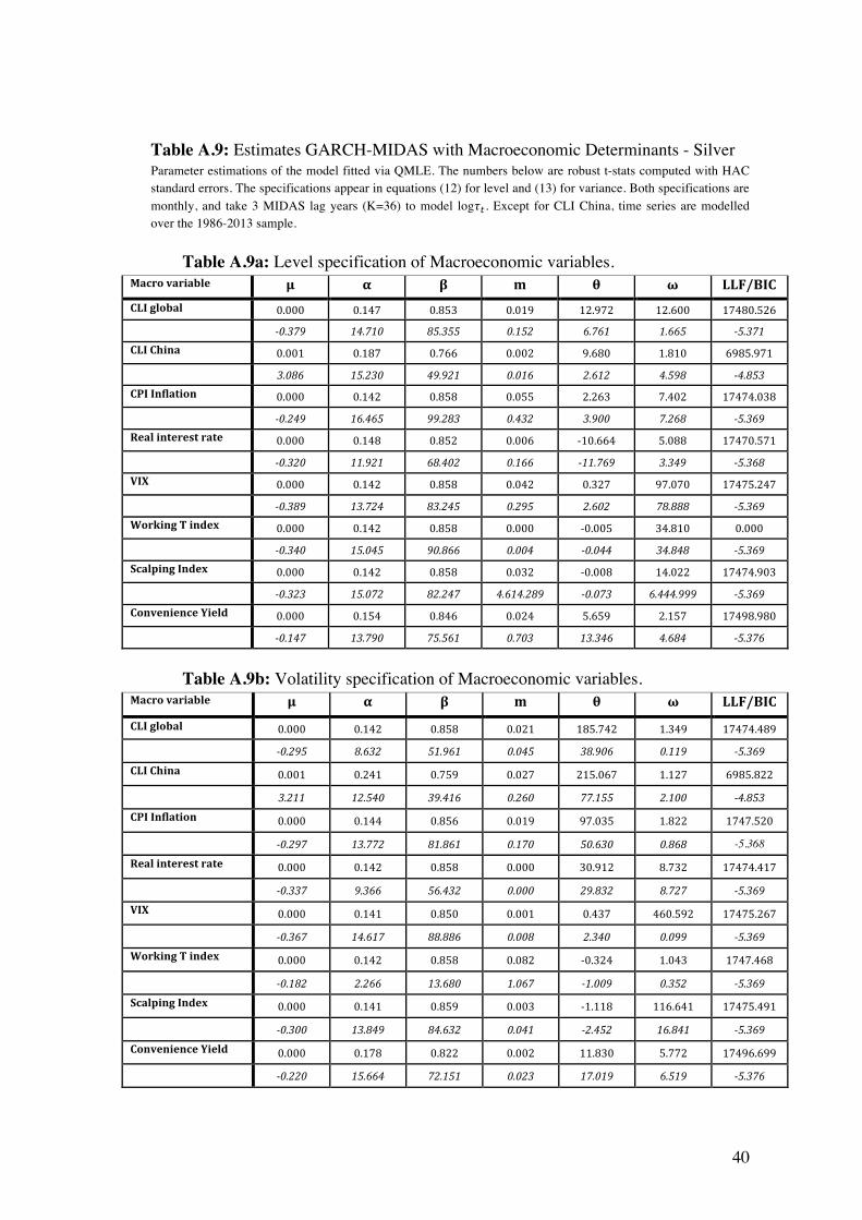
40

Table A.9: Estimates GARCH-MIDAS with Macroeconomic Determinants - Silver Parameter estimations of the model fitted via QMLE. The numbers below are robust t-stats computed with HAC standard errors. The specifications appear in equations (12) for level and (13) for variance. Both specifications are monthly, and take 3 MIDAS lag years (K=36) to model log!!. Except for CLI China, time series are modelled over the 1986-2013 sample.

Table A.9a: Level specification of Macroeconomic variables. Macro+variable+ μ+ α+ β+ m+ θ+ ω+ LLF/BIC+

CLI+global+ 0.000! 0.147! 0.853! 0.019! 12.972! 12.600! 17480.526!!! !0.379- 14.710- 85.355- 0.152- 6.761- 1.665- !5.371-CLI+China+ 0.001! 0.187! 0.766! 0.002! 9.680! 1.810! 6985.971!!! 3.086- 15.230- 49.921- 0.016- 2.612- 4.598- !4.853-CPI+Inflation+ 0.000! 0.142! 0.858! 0.055! 2.263! 7.402! 17474.038!!! !0.249- 16.465- 99.283- 0.432- 3.900- 7.268- !5.369-Real+interest+rate+ 0.000! 0.148! 0.852! 0.006! E10.664! 5.088! 17470.571!!! !0.320- 11.921- 68.402- 0.166- !11.769- 3.349- !5.368-VIX+ 0.000! 0.142! 0.858! 0.042! 0.327! 97.070! 17475.247!!! !0.389- 13.724- 83.245- 0.295- 2.602- 78.888- !5.369-Working+T+index+ 0.000! 0.142! 0.858! 0.000! E0.005! 34.810! 0.000!!! !0.340- 15.045- 90.866- 0.004- !0.044- 34.848- !5.369-Scalping+Index+ 0.000! 0.142! 0.858! 0.032! E0.008! 14.022! 17474.903!!! !0.323- 15.072- 82.247- 4.614.289- !0.073- 6.444.999- !5.369-Convenience+Yield+ 0.000! 0.154! 0.846! 0.024! 5.659! 2.157! 17498.980!!! !0.147- 13.790- 75.561- 0.703- 13.346- 4.684- !5.376-

Table A.9b: Volatility specification of Macroeconomic variables.

Macro+variable+ μ+ α+ β+ m+ θ+ ω+ LLF/BIC+

CLI+global+ 0.000! 0.142! 0.858! 0.021! 185.742! 1.349! 17474.489!!! !0.295- 8.632- 51.961- 0.045- 38.906- 0.119- !5.369-

CLI+China+ 0.001! 0.241! 0.759! 0.027! 215.067! 1.127! 6985.822!!! 3.211- 12.540- 39.416- 0.260- 77.155- 2.100- !4.853-

CPI+Inflation+ 0.000! 0.144! 0.856! 0.019! 97.035! 1.822! 1747.520!!! !0.297- 13.772- 81.861- 0.170- 50.630- 0.868- -5.368-

Real+interest+rate+ 0.000! 0.142! 0.858! 0.000! 30.912! 8.732! 17474.417!!! !0.337- 9.366- 56.432- 0.000- 29.832- 8.727- !5.369-

VIX+ 0.000! 0.141! 0.850! 0.001! 0.437! 460.592! 17475.267!!! !0.367- 14.617- 88.886- 0.008- 2.340- 0.099- !5.369-

Working+T+index+ 0.000! 0.142! 0.858! 0.082! E0.324! 1.043! 1747.468!!! !0.182- 2.266- 13.680- 1.067- !1.009- 0.352- !5.369-

Scalping+Index+ 0.000! 0.141! 0.859! 0.003! E1.118! 116.641! 17475.491!!! !0.300- 13.849- 84.632- 0.041- !2.452- 16.841- !5.369-

Convenience+Yield+ 0.000! 0.178! 0.822! 0.002! 11.830! 5.772! 17496.699!-- !0.220- 15.664- 72.151- 0.023- 17.019- 6.519- !5.376-

41

Table A.10: Estimates GARCH-MIDAS with Macroeconomic Determinants – Crude Parameter estimations of the model fitted via QMLE. The numbers below are robust t-stats computed with HAC standard errors. The specifications appear in equations (12) for level and (13) for variance. Both specifications are monthly, and take 3 MIDAS lag years (K=36) to model log!!. Except for CLI China, time series are modelled over the 1986-2013 sample.

Table A.10a: Level specification of Macroeconomic variables. Macro+variable+ μ+ α+ β+ m+ θ+ ω+ LLF/BIC+CLI+global+ 0.000! 0.116! 0.884! 0.002! E0.198! 6.670! 15935.063!!! 1.406- 13.713- 104.653- 0.012- !0.231- 6.643- !4.895-

CLI+China+ 0.001! 0.151! 0.849! 0.023! E23.651! 2.047! 7025.133!!! 2.636- 8.467- 47.536- 0.139- !6.812- 7.690- !4.881-CPI+Inflation+ 0.000! 0.116! 0.884! 0.021! E0.036! 13.537! 15935.054!!! 0.324- 15.374- 117.212- 0.150- !0.013- 12.486- !4.895-Real+interest+rate+ 0.000! 0.116! 0.884! 0.001! E3.899! 54.710! 15936.278!!! 0.445- 14.092- 107.899- 0.008- !3.794- 2.028- !4.895-VIX+ 0.000! 0.116! 0.884! 0.001! 0.771! 5.191! 15935.214!!! 1.959- 14.453- 109.765- 0.006- 1.384- 1.577- !4.895-Working+T+index+ 0.000! 0.116! 0.884! 0.002! 0.003! 1.112! 15935.064!!! 0.078- 1.039- 7.924- 0.001- 0.002- 0.256- !4.895-

Scalping+Index+ 0.000! 0.116! 0.884! 0.000! 0.027! 15.013! 15935.062!!! 0.247- 14.346- 109.549- 0.001- 0.073- 15.012- !4.895-

Convenience+Yield+ 0.000! 0.117! 0.883! 0.010! 4.503! 2.192! 15941.429!-- 2.049- 13.435- 100.924- 0.062- 6.289- 5.557- !4.897-

Table A.10b: Volatility specification of Macroeconomic variables.

Macro+variable+ μ+ α+ β+ m+ θ+ ω+ LLF/BIC+

CLI+global+ 0.000! 0.116! 0.884! 0.021! 139.204! 7.178! 15934.881!!! 1.886- 12.466- 94.844- 0.145- 31.719- 0.586- !4.895-

CLI+China+ 0.001! 0.167! 0.833! 0.000! 98.038! 1.537! 7015.511!!! 0.412- 20.589- 102.913- 0.000- 11.930- 0.107- !4.874-

CPI+Inflation+ 0.000! 0.116! 0.884! 0.001! 69.334! 1.001! 15935.171!!! 0.027- 8.446- 64.255- 0.058- 69.138- 0.037- !4.895-

Real+interest+rate+ 0.000! 0.116! 0.884! 0.021! 77.829! 23.355! 15936.119!!! 1.981! 15.080! 114.734! 0.186! 61.319! 2.189! E4.895!VIX+ 0.000! 0.116! 0.884! 0.002! 0.467! 22.734! 15935.188!

!! 0.622- 13.907- 106.004- 0.012- 7.483- 0.765- !4.895-

Working+T+index+ 0.000! 0.116! 0.884! 0.001! 0.021! 14.840! 15935.064!!! 0.803- 3.955- 30.186- 0.072- 0.001- 14.785- !4.895-

Scalping+Index+ 0.000! 0.116! 0.884! 0.002! 4.160! 240.668! 15935.257!

!! 1.713- 9.526- 72.764- 0.018- 1.265- 0.522- !4.895-

Convenience+Yield+ 0.000! 0.121! 0.879! 0.106! 5.311! 9.994! 15932.056!!! 1.903- 6.779- 49.234- 5.658- 26.109- 9.450- !4.894-

42

Table A.11: Estimates GARCH-MIDAS with Macroeconomic Determinants - Heating Parameter estimations of the model fitted via QMLE. The numbers below are robust t-stats computed with HAC standard errors. The specifications appear in equations (12) for level and (13) for variance. Both specifications are monthly, and take 3 MIDAS lag years (K=36) to model log!!. Except for CLI China, time series are modelled over the 1986-2013 sample.

Table A.11a: Level specification of Macroeconomic variables. Macro+variable+ μ+ α+ β+ m+ θ+ ω+ LLF/BIC+

CLI+global+ 0.001! 0.128! 0.872! 0.002! E6.861! 90.450! 16000.419!!! 0.103- 19.716- 134.469- 0.014- !2.845- 1.844- !4.915-

CLI+China+ 0.001! 0.111! 0.889! 0.002! E17.772! 1.593! 7118.873!!! 2.675- 11.244- 90.394- 0.014- !3.665- 4.360- !4.946-

CPI+Inflation+ 0.001! 0.128! 0.872! 0.002! 0.004! 6.927! 15999.706!!! 0.091- 18.194- 124.148- 0.018- 0.002- 1.255- !4.915-

Real+interest+rate+ 0.001! 0.128! 0.872! 0.020! E4.231! 54.784! 16001.415!!! 2.433- 18.731- 128.160- 0.161- !3.306- 1.452- !4.915-

VIX+ 0.000! 0.281! 0.719! 0.000! E1.503! 1.161! 16000.108!!! 2.320- 24.176- 141.669- 0.422- !0.740- 44.718- !4.915-

Working+T+index+ 0.001! 0.128! 0.872! 0.002! E0.001! 14.942! 15999.706!!! 2.153- 18.537- 126.500- 0.018- !0.006- 14.936- !4.915-

Scalping+Index+ 0.000! 0.815! 0.185! 0.000! E0.041! 5.123! 15444.234!!! 0.034- 0.138- 0.031- 0.000- !0.010- 0.164- !4.744-

Convenience+Yield+ 0.001! 0.126! 0.874! 0.000! 1.885! 2.441! 16000.141!!! 0.460- 13.123- 90.980- 0.001- 3.153- 7.571- !4.915-

Table A.11b: Volatility specification of Macroeconomic variables.

Macro+variable+ μ+ α+ β+ m+ θ+ ω+ LLF/BIC+CLI+global+ 0.001! 0.129! 0.871! 0.005! 263.867! 12.366! 15999.868!!! 1.932- 19.236- 129.657- 0.034- 210.765- 1.925- !4.915-CLI+China+ 0.001! 0.115! 0.885! 0.005! 121.374! 4.892! 7116.574!!! 1.056- 12.868- 98.617- 0.033- 83.324- 0.832- !4.944-CPI+Inflation+ 0.001! 0.131! 0.869! 0.005! 145.630! 5.364! 16000.792!!! 2.847- 17.392- 115.432- 0.031- 123.026- 3.396- !4.915-Real+interest+rate+ 0.001! 0.129! 0.871! 0.005! 57.138! 1.005! 15999.629!!! 2.755- 17.518- 118.680- 0.034- 51.773- 0.927- !4.915-VIX+ 0.001! 0.128! 0.872! 0.002! 0.537! 14.073! 15999.706!!! 2.320- 18.142- 123.801- 0.014- 16.565- 15.624- !4.915-

Working+T+index+ 0.001! 0.128! 0.872! 0.021! 0.406! 17.532! 15999.695!!! 2.333- 18.199- 124.151- 0.161- 0.795- 14.902- !4.915-

Scalping+Index+ 0.001! 0.129! 0.871! 0.033! 5.796! 2.875! 15999.706!!! 2.340- 17.832- 120.893- 0.271- 12.135- 3.532- !4.915-Convenience+Yield+ 0.001! 0.136! 0.864! 0.002! 6.270! 3.964! 16002.351!!! 1.836- 16.514- 105.000- 0.012- 5.211- 3.319- !4.916-

43

Table A.12: Correlation Matrix Commodity Log Returns Correlation coefficients for the commodity log returns over the 1986-2013 period.

Commodity Log returns

Wheat Soybeans Gold Silver Crude Heating

Wheat 1

Soybeans 0.417 1

Gold 0.131 0.156 1

Silver 0.164 0.205 0.728 1

Crude 0.116 0.141 0.216 0.208 1

Heating 0.119 0.117 0.192 0.178 0.738 1

44

Table A.13: C

orrelation Matrix M

acroeconomic V

ariables

Correlation coefficients for the m

acroeconomic variables over the 1986-2013 period.

C

orrelation Matrix

CLI

global C

PI inflation

Real int.

VIX

W

orking T Index Scalping Index

Convenience Y

ield

Macroeconom

ic Determ

inants W

heat Soybeans

Gold

Silver C

rude H

eating W

heat Soybeans

Gold

Silver C

rude H

eating W

heat Soybeans

Gold

Silver C

rude H

eating

CLI global

1

CPI inflation

0.123 1

Real int.

0.107 -0.364

1

VIX

-0.171

-0.038 -0.010

1

Working T

Index

Wheat

-0.015 0.155

0.048 -0.049

1

Soybeans 0.020

0.055 0.038

0.026 0.601

1

Gold

-0.022 0.009

0.056 -0.024

0.396 0.409

1

Silver -0.222

-0.031 -0.163

-0.012 0.141

0.103 0.287

1

Crude

-0.045 0.172

0.016 0.007

0.620 0.349

0.012 -0.166

1

Heating

0.018 0.102

0.045 -0.029

0.645 0.525

0.274 -0.021

0.597 1

Scalping Index

Wheat

-0.086 0.076

-0.129 0.050

-0.238 -0.207

-0.209 -0.130

-0.111 -0.191

1

Soybeans -0.044

0.048 -0.124

0.011 -0.310

-0.192 -0.222

-0.143 -0.199

-0.213 0.844

1

Gold

0.073 0.019

0.003 -0.114

0.172 0.098

0.178 0.127

-0.082 0.112

0.013 0.003

1

Silver -0.051

0.082 -0.056

-0.010 0.237

0.163 0.275

0.242 -0.059

0.040 0.113

0.022 0.400

1

Crude

0.067 0.008

0.014 -0.047

0.213 0.056

0.304 0.093

-0.101 0.204

-0.028 -0.024

0.534 0.286

1

Heating

0.073 -0.030

-0.018 -0.035

0.312 0.036

0.312 0.189

0.029 -0.001

-0.090 -0.122

0.473 0.209

0.541 1

Convenience

Yield

Wheat

-0.066 -0.099

0.082 0.128

0.112 0.042

0.053 0.077

0.073 -0.019

-0.237 -0.285

-0.111 -0.049

-0.006 0.082

1

Soybeans -0.029

0.087 0.030

-0.010 0.216

0.356 0.286

0.010 0.061

0.319 -0.132

-0.157 0.033

0.126 0.123

-0.122 0.202

1

Gold

-0.086 -0.222

0.233 -0.034

0.097 0.031

0.117 0.197

0.013 0.088

-0.176 -0.154

-0.049 -0.010

0.069 -0.023

0.161 -0.101

1

Silver -0.221

-0.196 0.117

0.151 0.071

0.008 0.139

0.206 0.020

-0.004 -0.126

-0.124 -0.094

-0.048 -0.017

0.027 0.202

0.064 0.659

1

Crude

-0.217 -0.458

0.252 0.144

0.059 0.096

0.001 0.126

0.033 0.145

-0.090 -0.078

-0.092 -0.046

0.001 -0.057

0.076 -0.041

0.174 0.183

1

Heating

-0.176 -0.357

0.212 0.102

0.145 0.166

0.005 0.134

0.058 0.208

-0.102 -0.098

-0.077 -0.035

0.023 -0.114

0.031 0.080

0.204 0.172

0.760 1

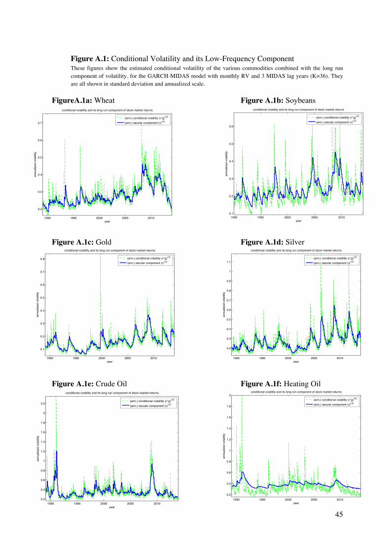
45

1990 1995 2000 2005 2010

0.2

0.3

0.4

0.5

0.6

0.7

year

annu

aliz

ed v

olat

ility

conditional volatility and its long run component of stock market returns

(ann.) conditional volatility (o*g)1/2

(ann.) secular component (o)1/2

Figure A.1: Conditional Volatility and its Low-Frequency Component These figures show the estimated conditional volatility of the various commodities combined with the long run component of volatility, for the GARCH-MIDAS model with monthly RV and 3 MIDAS lag years (K=36). They are all shown in standard deviation and annualized scale.

1990 1995 2000 2005 20100.1

0.2

0.3

0.4

0.5

0.6

yearan

nual

ized

vol

atilit

y

conditional volatility and its long run component of stock market returns

(ann.) conditional volatility (o*g)1/2

(ann.) secular component (o)1/2

1990 1995 2000 2005 2010

0.1

0.2

0.3

0.4

0.5

0.6

0.7

0.8

year

annu

aliz

ed v

olat

ility

conditional volatility and its long run component of stock market returns

(ann.) conditional volatility (o*g)1/2

(ann.) secular component (o)1/2

1990 1995 2000 2005 2010

0.2

0.3

0.4

0.5

0.6

0.7

0.8

0.9

1

1.1

year

annu

aliz

ed v

olat

ility

conditional volatility and its long run component of stock market returns

(ann.) conditional volatility (o*g)1/2

(ann.) secular component (o)1/2

1990 1995 2000 2005 20100.2

0.4

0.6

0.8

1

1.2

1.4

1.6

1.8

2

2.2

year

annu

aliz

ed v

olat

ility

conditional volatility and its long run component of stock market returns

(ann.) conditional volatility (o*g)1/2

(ann.) secular component (o)1/2

1990 1995 2000 2005 20100.2

0.4

0.6

0.8

1

1.2

1.4

1.6

1.8

2

year

annu

aliz

ed v

olat

ility

conditional volatility and its long run component of stock market returns

(ann.) conditional volatility (o*g)1/2

(ann.) secular component (o)1/2

FigureA.1a: Wheat

Figure A.1b: Soybeans

Figure A.1c: Gold

Figure A.1d: Silver

Figure A.1e: Crude Oil

Figure A.1f: Heating Oil

46

0 5 10 15 20 25 30 350

0.05

0.1

0.15

0.2

0.25

0.3

0.35optimal MIDAS weights

Figure A.2: Optimal Weighting Functions These figures show the optimal lag weights of GARCH-MIDAS with monthly RV and 3 MIDAS lag years, for all of the commodities. These models use 36 lagged monthly RV’s in MIDAS regression of !!. The horizontal axis of the figure is lag period in months; the vertical axis depicts the weights.

0 5 10 15 20 25 30 350

0.05

0.1

0.15

0.2

0.25

0.3

0.35optimal MIDAS weights

0 5 10 15 20 25 30 35 40 45 500

0.05

0.1

0.15

0.2

0.25

0.3

0.35optimal MIDAS weights

0 5 10 15 20 25 30 350

0.05

0.1

0.15

0.2

0.25

0.3

0.35optimal MIDAS weights

0 5 10 15 20 25 30 350

0.1

0.2

0.3

0.4

0.5

0.6

0.7optimal MIDAS weights

0 5 10 15 20 25 30 350

0.02

0.04

0.06

0.08

0.1

0.12optimal MIDAS weights

FigureA.2a: Wheat

Figure A.2b: Soybeans

Figure A.2c: Gold

Figure A.2d: Silver

Figure A.2e: Crude Oil

Figure A.2f: Heating Oil

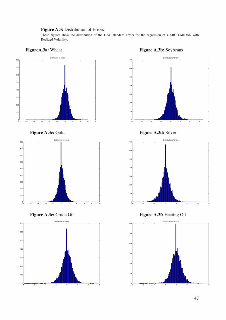
47

Figure A.3: Distribution of Errors These figures show the distribution of the HAC standard errors for the regression of GARCH-MIDAS with Realized Volatility.

−12 −10 −8 −6 −4 −2 0 2 4 6 80

100

200

300

400

500

600

700

800Distribution of errors

−8 −6 −4 −2 0 2 4 6 80

100

200

300

400

500

600

700Distribution of errors

−10 −8 −6 −4 −2 0 2 4 6 8 100

100

200

300

400

500

600

700

800

900Distribution of errors

−6 −4 −2 0 2 4 6 80

100

200

300

400

500

600

700Distribution of errors

−8 −6 −4 −2 0 2 4 60

100

200

300

400

500

600

700Distribution of errors

−8 −6 −4 −2 0 2 4 60

100

200

300

400

500

600Distribution of errors

FigureA.3a: Wheat

Figure A.3b: Soybeans

Figure A.3c: Gold

Figure A.3d: Silver

Figure A.3e: Crude Oil

Figure A.3f: Heating Oil

48

Figure A.4: Monthly Macroeconomic Variables – Levels These figures show macroeconomic level variables used in the GARCH-MIDAS with macroeconomic variables as specified in equation (12). Except for CLI China, time series data are showed over the 1986-2013 sample. The commodity specific macroeconomic variables (i.e. Working-T, Scalping and convenience yield) are omitted due to space limitations.

1990 1995 2000 2005 2010−8

−6

−4

−2

0

2

4

6x 10−3 CLI global

year2005 2010

−0.015

−0.01

−0.005

0

0.005

0.01

CLI china

year

1990 1995 2000 2005 2010

−0.015

−0.01

−0.005

0

0.005

0.01

CPI inflation

year1990 1995 2000 2005 2010

−0.01

−0.005

0

0.005

0.01

0.015Real interest rate

year

1990 1995 2000 2005 2010

−0.4

−0.2

0

0.2

0.4

0.6

0.8

1

1.2

VIX

year

Figure A.4a: %growth CLI Global

Figure A.4b: %growth CLI China

Figure A.4c: CPI inflation

Figure A.4d: Real interest rate growth

Figure A.4e: Change in VIX

49

Figure A.5: Monthly Macroeconomic Variables – Volatility These figures show macroeconomic volatility variables used in the GARCH-MIDAS with macroeconomic variables as specified in equation (13). Data is shown as squared terms of volatility (variance). Except for CLI China, time series data are showed over the 1986-2013 sample. The commodity specific macroeconomic variables (i.e. Working-T, Scalping and convenience yield) are omitted due to space limitations.

1990 1995 2000 2005 2010

1

2

3

4

5

6

x 10−6 CLI global

year

2005 2010

0.5

1

1.5

2

2.5

3

3.5

x 10−5 CLI china

year

1990 1995 2000 2005 2010

0.2

0.4

0.6

0.8

1

1.2

1.4

1.6

1.8

2

2.2x 10−4 CPI inflation

year1990 1995 2000 2005 2010

0.2

0.4

0.6

0.8

1

1.2

1.4

1.6

1.8

2

x 10−4 Real interest rate

year

1990 1995 2000 2005 2010

0.2

0.4

0.6

0.8

1

1.2

VIX

year

Figure A.4a: %growth CLI Global

Figure A.4b: %growth CLI China

Figure A.4c: CPI inflation

Figure A.4d: Real interest rate growth

Figure A.4e: Change in VIX