Commodity Covariance Contracting

8/6/2019 Commodity Covariance Contracting

http://slidepdf.com/reader/full/commodity-covariance-contracting 1/18

Commodity Covariance Contracting

Peter Carr, Principal

Banc of America Securities

Anthony Corso, Managing Director

Sithe Energies, Inc.

Abstract

We introduce covariance swaps and show how to replicate one between two futures prices by static positionsin spread and standard options coupled with dynamic trading in futures and bonds.

Current Version: May 20, 2001File Reference: ccc2pres.tex

Tuesday, May 22, 2001 Risk Course on Correlation New York, NY



Review of Variance Swaps

• A variance swap is a contract which pays the realized variance of the returns

of a specified underlying asset over a specified period of time.

• Several authors have shown that under certain conditions, the payoffs to

a continuously monitored variance swap can be synthesized by combining

continuous trading in the underlying with static positions in standard op-

tions maturing with the swap.

• While the development of a replication strategy for variance swaps repre-

sents a significant theoretical advance, there are at least three problems

with the proposed replication strategy:

1. The strategy replicates perfectly only if there are no jumps in the un-

derlying.

2. The strategy assumes that the variance swap is continuously monitored

even though all variance swaps are discretely monitored in practice.

3. The strategy requires continuous trading in the underlying which is

problematic in the presence of transactions costs and market closings.

2



Price Variance Swaps

• We propose a solution which addresses all three drawbacks described on

the previous page.

• By changing the definition of variance in the swap from the realized vari-

ance of returns to the realized variance of price changes, we show that the

new payoff can be perfectly replicated in the presence of jumps, discrete

monitoring, and discrete trading opportunities.

• We further show that a contract paying the realized covariance of price

changes can also be synthesized in this setting.

3



Using Spread Options

• We illustrate our results in the context of commodity options as the mar-

kets for these structures have many of the features which we require. In

particular, to synthesize covariance swaps, we use spread options, which

represent one of the few options written on two assets and listed on an

organized exchange.

• The standard papers on the valuation of spread options assume that the

covariance between the two commmodities in the spread is constant.

• We assume that the covariance between the two commodities is random, and

furthermore that the stochastic process governing covariance is unknown.

• Rather than price spread options in terms of a fixed covariance, we turn the

problem around and show how the covariance between the price changes in

two commodity futures can be traded, given the ability to trade dynamicallyin the futures and to take static positions in spread options and in options

written on each component of the spread.

4



Review of Static Hedging Using Options

• Consider a single period setting in which investments are made at time t0

with all payoffs received at time tn.

• We assume there exists a futures market in a commodity for delivery at

some date T ≥ tn.

• We also assume that markets exist for European-style futures options of allstrikes.

• Note that listed futures options are generally American-style. However, by

setting T = tn, the underlying futures will converge to the spot at tn and

so the assumption is that there exists European-style spot options in this

special case.

• The above market structure allows investors to create any smooth functionf (F n) of the terminal futures price F n by taking a static position at time 0

in options.

5



Constructing the Static Hedge

• When the theory of static hedging is used to generate desired volatility

exposures, only the second derivative of the payoff affects such exposures.

• Consequently, we will always choose f so that its value and slope vanish at

the initial futures price F 0 (i.e. f (F 0) = f (F 0) = 0).

• In this case, any twice differentiable payoff can be spanned by the followingposition in out-of-the-money options:

f (F n) = F 0−

0f (K )(K − F T )

+dK + ∞

F 0+f (K )(F T − K )+dK.

• In words, to create a twice differentiable payoff f (·) with value and slope

vanishing at F 0, buy f (K )dK puts at all strikes less than F 0 and buy

f (K )dK calls at all strikes greater than F 0.

6



Valuing the Static Hedge

• Recall the decomposition of f (·) into payoffs from puts and calls:

f (F n) = F 0−

0f (K )(K − F T )

+dK + ∞

F 0+f (K )(F T − K )+dK.

• In the absence of arbitrage, a similar decomposition must prevail among

the initial values. Specifically, if we let V f

0 , P 0(K ), and C 0(K ) denote the

initial prices of the payoff f (·), the put, and the call respectively, then theno arbitrage condition requires that:

V f

0 = F 0−

0f (K )P 0(K )dK +

∞F 0+

f (K )C 0(K )dK.

• Thus, the value of an arbitary payoff can be obtained from the option prices.

7



Application to Spread Options

• Given the spectrum of European options on the spread of two futures prices

S = F 1 − F 2, one can also create any smooth function of this spread g(S )

• If we assume that the value and slope vanish at the initial spread S 0 ∈

i.e. g(S 0) = g(S 0) = 0, then the analogous expression for the value of this

payoff is:

V g

0 = S 0−

−∞f (K )P s0 (K )dK +

∞S 0+

f (K )C s0(K )dK,

where P s0 (K ) and C s0(K ) are the initial prices of European put and call

spread options struck at K .

• Note that no assumptions were made regarding the stochastic processes

governing the futures prices.

8



Creating a Variance Contract

• Consider a finite set of discrete times {t0, t1, . . . , tn} at which one can trade

futures contracts.

• Let F i denote the price traded at on day i, for i = 0, 1, . . . , n. By day n, a

standard estimator of the realized annualized variance of price changes will

be:

Var(F ) ≡ N n

ni=1

(F i − F i−1)2,

where N is the number of trading days in a year.

• We next demonstrate a strategy whose terminal payoff matches the above

estimator of variance.

9



Derivation

• Recall that the objective is to find a trading strategy with final payoff of

Var(F ) ≡N

n

ni=1

(F i − F i−1)2,

where N is the number of trading days in a year.

• By Taylor’s series, we note that:F 2i = F 2i−1 + 2F i−1(F i − F i−1) + (F i − F i−1)2, i = 1, . . . , n .

• Re-arranging and summing implies:n

i=1(F 2i − F 2i−1) −

ni=1

2F i−1(F i − F i−1) =n

i=1(F i − F i−1)2, i = 1, . . . , n .

• The first sum on the left telescopes to F 2n

− F 20

. Thus, multiplying both

sides by N n

implies:

Var(F ) =N

n(F 2n − F 20 ) −

ni=1

2N

nF i−1(F i − F i−1).

10



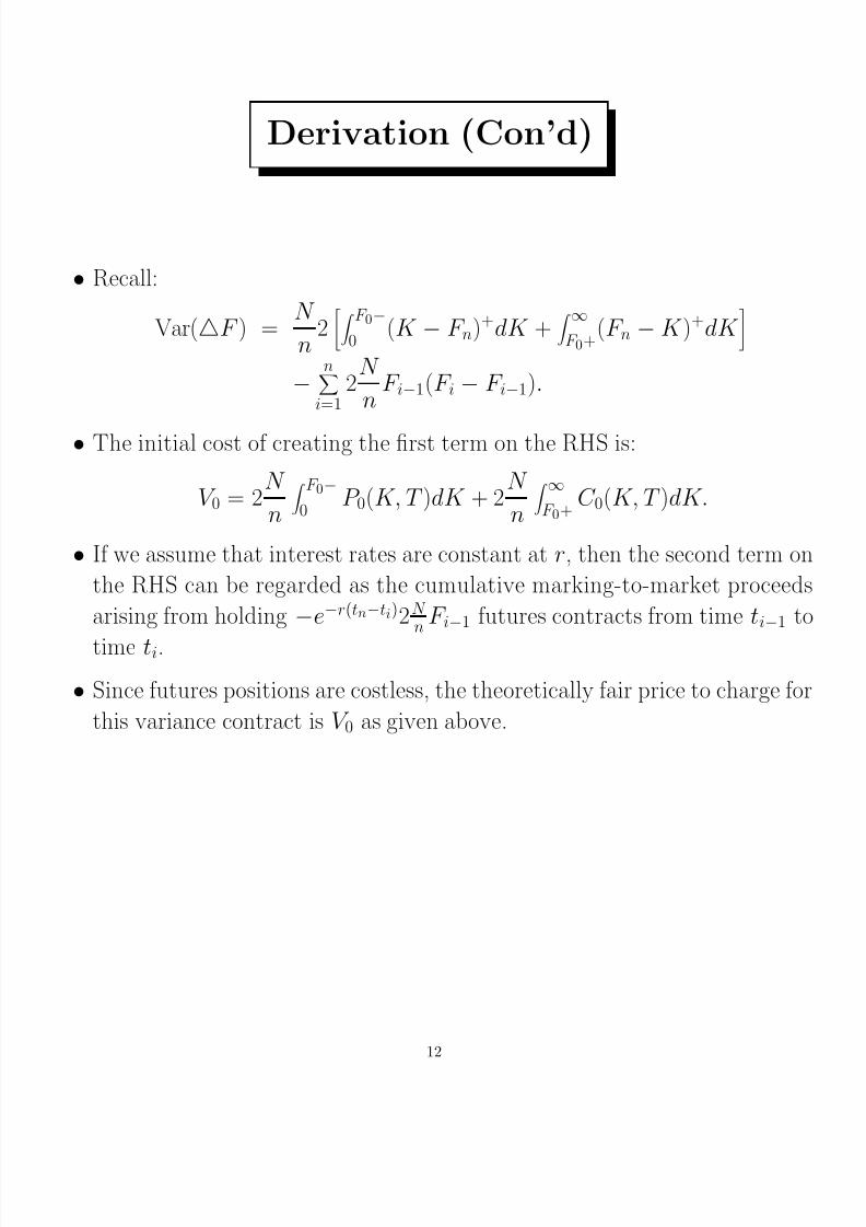
Derivation (Con’d)

• Recall:

Var(F ) =N

n(F 2n − F 20 ) −

ni=1

2N

nF i−1(F i − F i−1).

• The first term on the RHS can be regarded as a function φ(·) of F n, where

φ(F ) ≡ N n

(F − F 0)2.

• The first derivative is given by:

φ(F ) =N

n2(F − F 0).

• Thus, the value and slope both vanish at F = F 0. Hence, the payoff φ(F n)

can be replicated using options. The number of options held at each strikeis proportional to the second derivative of φ, which is simply:

φ(F ) =N

n2.

• Substitution implies:

Var(F ) =N

n

2 F 0−

0

(K − F n)+dK + ∞

F 0+

(F n − K )+dK −

ni=1

2N

nF i−1(F i − F i−1).

11



Derivation (Con’d)

• Recall:

Var(F ) =N

n2 F 0−

0(K − F n)+dK +

∞F 0+

(F n − K )+dK

−n

i=12

N

nF i−1(F i − F i−1).

• The initial cost of creating the first term on the RHS is:

V 0 = 2N

n

F 0−

0P 0(K, T )dK + 2

N

n

∞F 0+

C 0(K, T )dK.

• If we assume that interest rates are constant at r, then the second term on

the RHS can be regarded as the cumulative marking-to-market proceeds

arising from holding −e−r(tn−ti)2N n

F i−1 futures contracts from time ti−1 to

time ti.

• Since futures positions are costless, the theoretically fair price to charge for

this variance contract is V 0 as given above.

12



An Interpretation

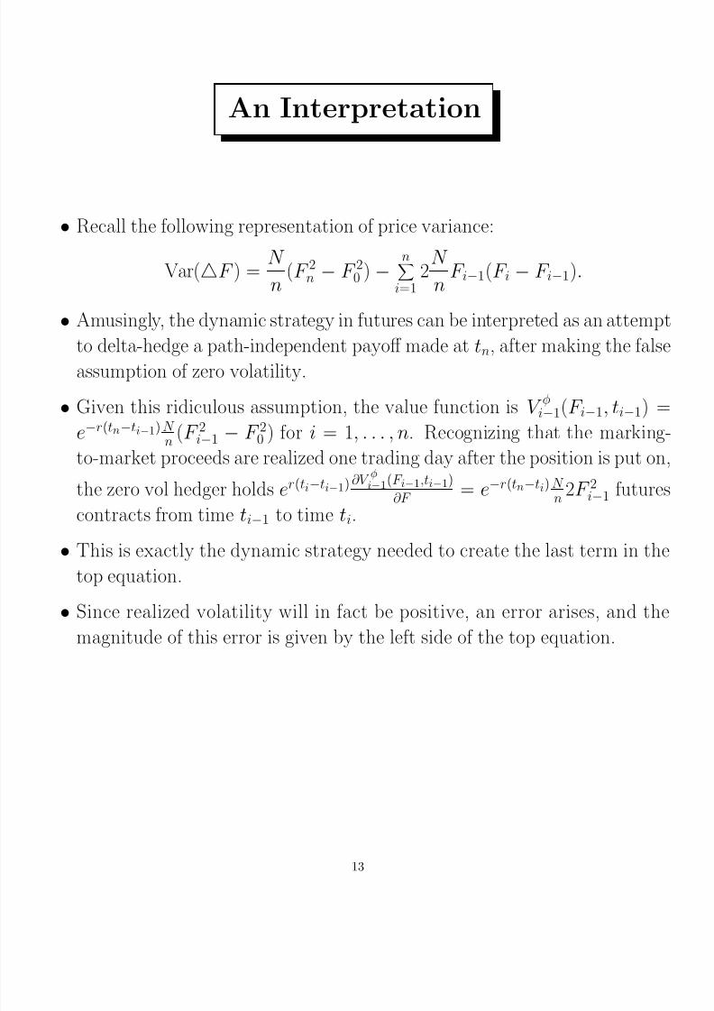
• Recall the following representation of price variance:

Var(F ) =N

n(F 2n − F 20 ) −

ni=1

2N

nF i−1(F i − F i−1).

• Amusingly, the dynamic strategy in futures can be interpreted as an attempt

to delta-hedge a path-independent payoff made at tn, after making the falseassumption of zero volatility.

• Given this ridiculous assumption, the value function is V φ

i−1(F i−1, ti−1) =

e−r(tn−ti−1) N n

(F 2i−1 − F 20 ) for i = 1, . . . , n. Recognizing that the marking-

to-market proceeds are realized one trading day after the position is put on

the zero vol hedger holds er(ti−ti−1) ∂V φi−1(F i−1,ti−1)

∂F = e−r(tn−ti) N

n2F 2i−1 futures

contracts from time ti−1 to time ti.

• This is exactly the dynamic strategy needed to create the last term in the

top equation.

• Since realized volatility will in fact be positive, an error arises, and the

magnitude of this error is given by the left side of the top equation.

13



Creating a Covariance Contract

• Recall that:

S i ≡ F 1,i − F 2,i, i = 0, 1, . . . , n

denotes the spread on day ti, where F 1,i and F 2,i denote the contempora-

neous futures prices of the two components of the spread.

• We now show how to create a contract paying Cov(F 1, F 2) ≡N

n

ni=1(F 1,i−

F 1,i−1)(F 2,i−F 2,i−1) at time tn by combining static positions in options with

dynamic trading in the underlying futures.

14



Creating a Covariance Contract

• Recall the well-known result that:

Var(S ) = Var((F 1−F 2)) = Var(F 1)−2Cov(F 1, F 2)+Var(F 2).

• Re-arranging this expression gives:

Cov(F 1, F 2) = −1

2Var(S ) +1

2Var(F 1) +1

2Var(F 2).

• Thus, one can synthesize a covariance swap by selling half a variance swap

on the spread and buying half a variance swap on each of the spread com-

ponents.

15



Static Option & Dynamic Futures Positions

• Recall that one can synthesize a covariance swap by selling half a variance

swap on the spread and buying half a variance swap on each of the spread

components:

Cov(F 1, F 2) = −1

2Var(S ) +

1

2Var(F 1) +

1

2Var(F 2).

• As these variance swaps are unlikely to be explicitly available, they can be

synthesized. Substitution implies:

Cov(F 1, F 2) = −N

n

S 0−

0(K − S n)+dK +

∞S 0+

(S n − K )+dK

+n

i=1

N

nS i−1(S i − S i−1)

+N

n

F (1)0 −

0(K − F (1)

n )+dK + ∞

F (1)0 +

(F (1)n − K )+dK

−n

i=1

N

nF

(1)i−1(F

(1)i − F

(1)i−1)

+N

n

F

(2)0 −

0(K − F (2)

n )+dK + ∞

F (2)0 +

(F (2)n − K )+dK

−n

i=1

N

nF

(2)i−1(F

(2)i − F

(2)i−1).

• The 2nd term on the RHS can be created by dynamic trading in futures on

the spread components:n

i=1

N

nS i−1(S i − S i−1) =

ni=1

N

nS i−1[(F

(1)i − F

(2)i ) − (F

(1)i−1 − F

(2)i−1)]

=n

i=1

N

nS i−1(F

(1)i − F

(1)i−1) −

ni=1

N

nS i−1(F

(2)i − F

(2i−

16



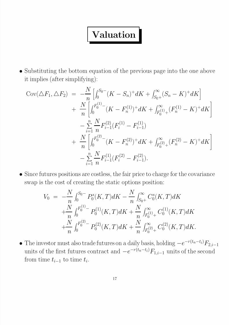
Valuation

• Substituting the bottom equation of the previous page into the one above

it implies (after simplifying):

Cov(F 1, F 2) = −N

n

S 0−

0(K − S n)+dK +

∞S 0+

(S n − K )+dK

+N

n

F (1)0 −

0

(K − F (1)n )+dK +

∞

F

(1)

0 +

(F (1)n − K )+dK

−n

i=1

N

nF

(2)i−1(F

(1)i − F

(1)i−1)

+N

n

F

(2)0 −

0(K − F (2)

n )+dK + ∞

F (2)0 +

(F (2)n − K )+dK

−n

i=1

N

nF

(1)i−1(F

(2)i − F

(2)i−1).

• Since futures positions are costless, the fair price to charge for the covariance

swap is the cost of creating the static options position:

V 0 = −N

n

S 0−

0P s0 (K, T )dK −

N

n

∞S 0+

C s0(K, T )dK

+N

n

F (1)0 −

0P

(1)0 (K, T )dK +

N

n

∞F

(1)0 +

C (1)0 (K, T )dK

+

N

n F

(2)0 −

0 P (2)0 (K, T )dK +

N

n ∞

F (2)0 + C

(2)0 (K, T )dK.

• The investor must also trade futures on a daily basis, holding −e−r(tn−ti)F 2,i−

units of the first futures contract and −e−r(tn−ti)F 1,i−1 units of the second

from time ti−1 to time ti.

17



Summary & an Extension

• We showed that by combining static positions in options with dynamic

trading in futures, investors can synthesize contracts paying the realized

variance of a commodity or paying the realized covariance between two

commodities.

• Importantly, these contracts were created without assuming anything about

the underlying price.

• It would be interesting to extend our results to other payoffs besides variance

and covariance. Indeed, Carr, Lewis, and Madan (2000) characterize the

entire set of continuously paid cash flows which can be spanned in our

structure.

• If interested, this paper (called On the Nature of Options) can be down-

loaded from:www.petercarr.net or

www.math.nyu.edu\carrp\research\papers

18

Commodity Covariance Contracting

Documents

Transcript of Commodity Covariance Contracting