Commodity-based Consumption Tracking Portfolio

and the Cross-section of Average Stock Returns

Kewei Hou∗ and Marta Szymanowska†

February 16, 2015

Abstract

We find that the projection of consumption growth on commodity futures re-

turns tracks the part of consumption that is priced in the cross-section of US stock

returns. When consumption betas are estimated using the commodity-based con-

sumption tracking portfolio, the Consumption CAPM (CCAPM) produces a sig-

nificant risk premiums between 50bp and 1% per year depending on the empiri-

cal specification. In contrast, we fail to find significant risk premiums when the

CCAPM is estimated using either non-traded consumption growth or stock- and

bond-based consumption tracking portfolios. Our results are robust to using ei-

ther portfolios or individual stocks in the asset pricing tests and to controlling for

firm-level return predictors such as size, book-to-market, and past returns.

JEL classification: G12, G13

Keywords: Commodities, Consumption Risk, CCAPM, Tracking Portfolios

∗Department of Finance, Fisher College of Business, Ohio State University, 2100 Neil Avenue, Colum-

bus, OH 43210. Phone: (614)292-0552. Email: hou.28@osu.edu.†Corresponding author. Department of Finance, Rotterdam School of Management, Erasmus Uni-

versity, P.O. Box 1738, 3000 DR Rotterdam, the Netherlands, email: mszymanowska@rsm.nl, phone:

+31104089607, fax: +31104089017.

1

1 Introduction

The standard consumption-based asset pricing model (CCAPM) developed by Rubinstein

(1976), Lucas (1978), and Breeden (1979) is a natural choice for analyzing the cross-

sectional differences in average returns on financial assets. The model builds on an

idea that assets should carry higher risk premium if they pay off poorly in bad times

as measured by consumption growth. Hence a simple relation between consumption

growth and asset returns captures the implications of the multifactor intertemporal asset

pricing models (Breeden (1979)). Despite being theoretically appealing, the empirical

performance of the CCAPM has proven unsatisfactory (Campbell and Cochrane (2000)).

To address this deficiency, the literature has proposed non-standard assumptions (e.g.,

infrequent decision making of Parker and Julliard (2005) or Jagannathan and Wang

(2007)); more sophisticated preference structures (e.g., Campbell and Cochrane (1999),

Bansal and Yaron (2004), Yogo (2006)); or hard to detect features of the consumption

data (e.g., small but persistent component of the dividend process in the long run risk

models as in Bansal and Yaron (2004)). But given that Lettau and Ludvigson (2005)

show that the standard CCAPM should hold as a good approximation even if economies

are driven by more sophisticated preference structures, the poor empirical performance

of the CCAPM is still puzzling.

In this paper we offer a new measure of consumption risk that could potentially solve

this puzzle. In particular, we replace the consumption growth in the CCAPM model

with its tracking portfolios. Balduzzi and Robotti (2008) show that the risk premiums

estimates are more reliable when noisy non-traded factors are replaced by their projections

on the span of asset returns. What is novel here is that we construct the consumption

tracking portfolios not from stocks and bonds, as is common in the literature, but from

2

commodity futures contracts.

It is natural to think that commodities should contain price relevant consumption

information, since certain commodities are directly related to aggregate consumption

itself. For example, based on the data from the National Income and Product Accounts

(NIPA) commodities constitute around 40% of the personal consumption expenditures

(PCE) with energy commodities accounting for 4%, food commodities for 15%, and other

commodities for 21%. Further, commodity futures are known to be good inflation hedges1

and hence may be used for hedging real consumption risk. Finally, futures prices being

forward looking are often viewed as informative about future economic activity, and are

known to facilitate price discovery (e.g., Working (1948), Garbade and Silber (1983), and

Hong and Yogo (2012)). Our goal in this paper is to construct a proxy that captures the

part of consumption that is relevant for pricing and we posit that the commodity futures

returns contain more price relevant consumption information than stocks and bonds.

We find that the fraction of variation in consumption growth captured by our commodity-

based consumption tracking portfolios is similar to that of the more traditional stock-

based tracking portfolios but higher than that of bond-based tracking portfolios. More

importantly, betas with respect to the commodity-based consumption tracking portfolios

(but not those related to the stock and bond-based tracking portfolios) are significantly

priced in the cross section of stocks returns, with an average risk premium ranging be-

tween 50bp and 1% per year depending on the empirical specifications. Our results

are robust to using either portfolios or individual stocks in the asset pricing tests and to

controlling for firm-level return predictors such as size, book-to-market, and past returns.

Our paper is part of a growing literature that seeks to improve the performance of

1See e.g., Breeden (1980), Bodie (1983), Greer (2000), Erb and Harvey (2006),Gorton and Rouwen-horst (2006), Attie and Roache (2009), and Bekaert and Wang (2010).

3

the standard consumption-based asset pricing model. Early studies find little support for

the CCAPM using non-traded consumption data. For example, Hansen and Singleton

(1982) reject the model and Hansen and Jagannathan (1997) find large pricing errors.

Breeden, Gibbons, and Litzenberger (1989) construct consumption mimicking portfolios

from stocks and bonds but find that they do not change the poor performance of the

CCAPM using monthly data. However, recent studies show more promises for the model.

For example, Jagannathan and Wang (2007) show that the CCAPM performs better in

annual data when consumption growth is measured over the fourth quarters. Savov

(2011) proxies for consumption using data on municipal solid waste and finds that the

garbage growth is priced in the cross-section of US and international portfolio returns.

Da and Yun (2010) and Chen and Lu (2012) follow in his footsteps and find similar

results when using electricity consumption and carbon dioxide emissions to proxy for

consumption. This paper is in the same spirit, but we focus solely on traded portfolios

when constructing our proxy for consumption risk.

The rest of the paper is organized as follows. In section 2 we introduce the standard

beta representation of the CCAPM and discuss the construction of the consumption

tracking portfolios. In Section 3 we describe our data. Section 4 shows the ability of our

tracking portfolios to capture the dynamics of consumption data and reports the results

of the asset pricing tests. Section 5 summarizes and concludes.

2 The Consumption-CAPM and consumption track-

ing portfolios

2.1 The Consumption-CAPM

Rubinstein (1976), Lucas (1978), and Breeden (1979) develop the Consumption-CAPM

4

(CCAPM) where the risk of a security is determined by its covariance with consumption

growth. Assuming that the period utility function has a constant relative risk aversion

γ, the pricing kernel for the standard CCAPM takes the following form:

mt = δ

(CtCt−1

)−γ, (1)

where δ is the time discount factor,(

Ct

Ct−1

)is the consumption growth from time t − 1

to time t.

For the unconditional excess returns, ri,t, the above defined stochastic discount factor

yields

E [mtri,t] = 0 (2)

⇔ E [ri,t] = −Cov

[ri,t,∆c

−γt

]E[∆c−γt

] ,

where ∆ct =(

Ct

Ct−1

).

To derive a beta representation for this model we use a first order Taylor expansion of

∆c−γt around its mean to avoid assuming a joint log-normality of returns and consumption

growth

E [ri,t] = λcβic (3)

βic =Cov [ri,t,∆ct]

V ar [∆ct]

where λc is the market price of consumption risk, λc = −γV ar [∆ct] /∆ct.

This is the standard beta representation of the CCAPM. The intuition is that investors

dislike securities that pay well in good times and poorly in bad times and will hence

demand higher risk premiums for holding those assets. If we measure those bad and

good states with consumption growth then the CCAPM predicts that assets with high

5

covariances with consumption growth should earn high expected returns.

2.2 The consumption tracking portfolios

One challenge in estimating equation (3) is the poor quality of the consumption data.

The common way of constructing ∆ct is to use data from NIPA tables which may be

biased due to methodological issues like interpolating, forecasting, and the incidence of

non-reporting. Also, theory implies that consumption risk is measured with respect to

aggregate consumption growth between two points in time. In practice, however, we

observe total expenditures on goods and services over a period of time. This creates a so

called ”summation (or time-aggregation) bias” (e.g., Breeden, Gibbons, and Litzenberger

(1989)). One way to avoid this problem would be to use higher frequency consumption

data, but these data are measured less precisely. Hence, the convention in the literature

is to use lower frequency data - mostly at quarterly (e.g., Lettau and Ludvison (2001))

or annual frequencies (Jagannathan and Wang (2007)).

Instead, we replace non-traded consumption growth in equation (3) with traded track-

ing portfolio that captures the price relevant consumption information. Tracking portfo-

lios have long been used in the asset-pricing literature. For example, Breeden, Gibbons,

and Litzenberger (1989) and Jagannathan and Wang (2007) use simple unconditional

tracking portfolios with fixed weights to mimic consumption growth and test the CCAPM.

Lamont (2001) shows how to construct the portfolio that instead maximizes the condi-

tional correlation between the span of asset returns and several economic factors such as

production growth, consumption growth, labor income growth, and inflation. Vassalou

(2003) uses Lamont’s method to construct a mimicking portfolio that captures news re-

lated to future GDP growth. Ferson, Siegel, and Xu (2006) study similar portfolios as

Lamont (2001) but they consider optimal time-varying portfolios weights in both uncon-

6

ditional and conditional setups. They find a potential improvement in the correlations

above the fixed-weight portfolios of more than 20% but the results are sensitive to the

estimation errors and errors in specifying the form of the data generating process. Alter-

natively, time-varying portfolio weights can be estimated using rolling window regressions

as in Ferson and Harvey (1991) who use tracking portfolios to assess the level of return

predictability captured by asset pricing models. In this paper, we use tracking portfolios

with fixed weights, which we estimate unconditionally and conditionally.

In particular, we follow Huberman, Kandel, and Stambaugh (1987) and construct

the fixed-weight portfolio that maximizes the unconditional correlation with the non-

traded consumption growth by projecting consumption growth onto the span of base

asset returns, augmented with a constant

∆ct = ν + φRt + εt, (4)

where ∆ct is the non-traded consumption growth, Rt is a vector of excess returns on the

base assets.

Since the consumption tracking portfolios capture the risk that arises due to the

changes in investment and consumption opportunities (Merton (1973), Breeden (1979)),

we want to incorporate conditioning information into the estimation of the tracking port-

folios. To this end we follow Lamont (2001) and extend equation (4) in the following

way

∆ct = ν + φRt + ϕzt−1 + εt, (5)

where zt−1 are predictive variables know one period before the returns are realized. The

underlying assumption is that time-varying conditional means of base asset returns are

linear functions of current information about the economic state that is captured with

7

zt−1.

In both the unconditional and conditional cases we define the consumption tracking

portfolio as CTPt = φRt.

3 Data

We use monthly data on consumption growth, asset returns, and predictive instruments

from January 1984 to December 2007.

We obtain consumption and population data from the Bureau of Economic Analysis

(BEA). We measure consumption growth as the percentage change in the seasonally

adjusted, aggregate, real per capita consumption expenditures on nondurable goods and

services from Section 2 of the National Income and Product Accounts (NIPA) tables.

We construct consumption tracking portfolios from three different sets of base assets:

stocks, bonds, and commodity futures contracts. The stock-based consumption tracking

portfolio (CTPs) uses as base assets the value-weighted CRSP index and the 17 value-

weighted industry portfolios downloaded from Ken French’s data library. The bond-based

consumption tracking portfolio (CTPb) uses ten corporate bond portfolios (intermediate-

and long-term returns for four investment grades and one junk grade) and two government

bond portfolios (intermediate- and long-term). All bond data are retrieved from the

WRDS.

To construct the commodity-based consumption tracking portfolio (CTPc), we use

data on 84 futures contracts across 20 different commodities and up to five different ma-

turities obtained from the Futures Industry Institute (FII) Data Center and RC Research.

We sort those contracts into four sectors 2 (Energy, Meats, Metals, and Agriculture) and

five maturities, which we then use to create 20 equally-weighted portfolios as base assets

2Similar classification was used in Hong and Yogo (2012).

8

for the consumption tracking portfolio.3 Following common practice in the literature, we

calculate futures returns using a rollover strategy with the nearest-to-maturity futures

contracts. At the beginning of the month prior to the delivery month, we roll-over the

position from the nearest-to-maturity contract to the contract with the next nearest de-

livery month. Prices of futures observed in the last month prior to and during the delivery

month are excluded from the analysis to avoid irregular price behavior that is common

due to investors rolling over their positions. Table 1 lists the 20 different underlying

commodities, the delivery months for each contract, and the name of the exchange where

each contract is traded. We also report the first observation for each commodity contract

for all nearby series used. We choose 1984 as the starting point of our analysis because it

ensures that we have at least ten commodity contracts and a minimum of two contracts

in each sector.

Insert Table 1 around here

The descriptive statistics for the base assets are shown in Table 2. Panel A shows that

the commodity portfolios exhibit substantial variation in average returns across sectors.

For example, for the nearest maturity contracts, the average returns vary from a high

of 1.35% for the Energy sector to a low -0.03% for the Agriculture sector. Energy and

Metals have a downward-sloping term structure in average returns, while Meats and

Agriculture have a hump-shape relation between average return and maturity. There

is also considerable variation in volatility across sectors, with the Energy sector being

almost twice as volatile as the other three sectors. The relation between volatility and

maturity is fairly flat across sectors. Panel B of Table 2 shows that the average returns of

the stock portfolios vary from a high of 1.09% for the CRSP index to a low of 33bps for

the Durable industry and the volatility varies from a high of 7.50% for the Steel industry

3We get similar results when we use open-interest to weight the contracts within each sector.

9

to a low 3.93% for the Utility industry. Panel C of Table 2 shows more muted differences

in average returns and volatility across bond portfolios. The average returns (volatility)

vary from a high of 0.56% (2.55%) for long-term junk bonds to a low 20bps (0.86%) for

intermediate-term government bonds.

Insert Table 2 around here

To capture conditioning information, we select seven instruments commonly used in

the asset pricing literature.4 Term spread (TERM) is the yield spread between ten- and

one-year government bonds. Default spread (DEF) is the yield spread between Moody’s

Baa- and Aaa-ranked corporate bonds. Unexpected inflation (UI) is measured as the

difference between the realized inflation and the one month t-bill rate (proxy for the

market’s short-term inflation expectation). Change in the short term-expected inflation

(ESR) is measured as the change in the one month t-bill rate. Change in the long-term

expected inflation (ELR) is measured as the change in ten-year government bond yield.

We also include the CRSP value-weighted market index (MARKET) and the dividend

yield on S&P 500 index (DY) as instruments.

For our asset-pricing tests, we use the independently-sorted five size, five book-to-

market, five momentum, and five industry portfolios downloaded from Ken French’s data

library as test assets. Table 3 reports the descriptive statistics of the test asset portfolios.

Panel A shows that these test portfolios produce substantial cross-sectional dispersion in

average returns. For example, the momentum winner portfolio earn an average excess

return of close to 1% per month, whereas the momentum loser portfolio earn only 10

bps per month. Large return differences are also observed across the book-to-market

4See, e.g., Fama and Schwert (1977), Ferson and Harvey (1991), Pesaran and Timmermann (1995),Kirby (1998), Erb and Harvey (2006), and Hong and Yogo (2012).

10

portfolios, from a high of 0.89% per month for the growth portfolio to a low of 0.60%

per month for the value portfolio. Panel B reports the standard deviations of the test

portfolios, which also show sizable variation. They vary from a high of 6.61% per month

for the momentum loser portfolio to a low of 3.86% per month for the Manufacturing

industry portfolio. Finally, Panel C reports the consumption betas of the test portfolios.

The betas often go in the wrong direction in explaining the average return differences.

For example, the value portfolio and the momentum winner portfolio earn higher returns

but have lower consumption betas than the growth portfolio and the momentum loser

portfolio, respectively. These results are consistent with the poor performance of the

CCAPM reported in previous studies (Campbell and Cochrane (2000) and references

therein).

Insert Table 3 around here

In addition to using test portfolios, we also use individual stocks from the CRSP

universe (sharecodes 10 or 11, i.e., excluding ADRs, closed-end funds, and REITs) in our

asset pricing tests. This is to ensure that our results are not affected by the potential

concerns about the portfolio-based approach (see, e.g., Lewellen, Nagel, and Shanken

(2010) and Ang, Liu, and Schwarz (2010)). To the best of our knowledge, our paper is

the first to use individual stocks to test the CCAPM.

4 Results

We start out by discussing the ability of our tracking portfolios to capture the consump-

tion growth dynamics. We then analyze the pricing implications of those consumption

tracking portfolios for the cross-section of average returns.

11

4.1 How good are our tracking portfolios?

We estimate the consumption tracking portfolios by projecting consumption growth onto

three different sets of base assets (stocks, bonds, and commodity futures returns), as

given in equations (4) and (5). Table 4 reports the summary statistics of the consump-

tion tracking portfolios. Panel A shows that the average returns of all three unconditional

tracking portfolios are identical to the mean level of consumption growth, but the aver-

age returns of the conditional tracking portfolios are lower than the mean consumption

growth. Both unconditional and conditional tracking portfolios are less volatile than raw

consumption growth, with the monthly standard deviation ranging between 0.06 and

0.09% (compared with 0.29% for consumption). Consequently, the tracking portfolios

capture less than a quarter of the variation of consumption growth. This is in line with

consumption data being noisy and biased due to interpolating, incidence of non-reporting

or data revisions as is commonly observed in the NIPA tables. Comparing across tracking

portfolios, the stock-based and commodity-based tracking portfolios capture around 9%

of the consumption growth variation unconditionally and 14% conditionally, whereas the

bond-based consumption tracking portfolio captures 4% of the unconditional variation

and 8% of the conditional variation. The p-values for the joint significance of all base

assets reported in the last row of Panel A indicate that stocks and commodity futures

are important in capturing consumption dynamics, while bonds are not (the individ-

ual coefficients on the base assets are reported in Panel C). Panel B of Table 4 reports

the correlations between the consumption tracking portfolios and consumption growth.

Consistent with the results from Panel A, both the stock-based and commodity-based

tracking portfolios are more strongly correlated with consumption growth (correlations

12

around 30%) than the bond-based tracking portfolios (correlation around 20%).

Insert Table 4 around here

To sum up, the evidence from Table 4 suggests that the stock-based and commodity-

based tracking portfolios capture consumption dynamics to a similar degree, while the

bond-based tracking portfolio does a poorer job. Next, we examine the pricing implica-

tions of these tracking portfolios.

4.2 Portfolio Results

We first study the ability of the CCAPM to explain the average returns of the 20 test

portfolios (five size, five book-to-market, five momentum, and five industry portfolios).

Panel A of Table 5 reports the average returns and the full-sample consumption betas, βi,c,

as well as the betas with respect to the unconditional consumption tracking portfolios,

βi,CTP , for the 20 test portfolios. The table shows that the CTPc betas line up fairly well

with the average returns, whereas the other betas do not. For example, the CTPc beta

increases monotonically from -0.238 for the momentum loser portfolio to 8.718 for the

momentum winner portfolio. On the other hand, the consumption beta first decreases

from 2.983 for the momentum loser portfolio to 1.155 for momentum quintile four and

then increases to 2.240 for the momentum winner portfolio, exhibiting a U-shape pattern.

Similarly, the CTPs beta decreases from 30.760 for the momentum loser portfolio to

15.000 for momentum quintile four and then increases to 24.701 for the momentum winner

portfolio. Panel A also shows that the consumption betas and CTPc betas are of similar

magnitude while the CTPs and CTPb betas are one order of magnitude larger.

Insert Table 5 around here

13

Panels B and C of Table 5 report the results of the portfolio-level asset pricing tests.

Panel B reports the average coefficients and their associated t-statistics from monthly

Fama and MacBeth (1973) cross-sectional regressions. In Panel C, we estimate the

stochastic discount factor representation of the form

E[(1− b′CTPj) rt] = 0, (6)

and report the estimated coefficients, b, with their associated t-statistics, as well as the

J-test for the overidentifying restrictions. We use fully iterated efficient GMM estimator

of Hansen (1982) but our results are robust to using first-stage estimator or HJ-weighting

matrix.

We start with the CCAPM estimated using the consumption growth itself. Consistent

with numerous previous studies, we do not find much support for this model. Panel

B shows that the average Fama-MacBeth regression coefficient on consumption beta is

negative (-0.09%) and statistically insignificant (t-stat=-0.93), and the J-test in Panel C

rejects the model with a p-value of 0.01.

The performance of the model is much improved when we replace the non-traded

consumption growth with it’s tracking portfolio constructed from commodity futures

contracts. In Panel B, the average Fama-MacBeth coefficient on CTPc beta is positive

and significant at 0.07% (t-stat=2.60) per month, which implies a risk premium of more

than 80 bps per annum. In addition, the adjusted-R2 increases sharply from 12% for the

baseline case using consumption growth to 56%. In Panel C, the J-test fails to reject the

hypothesis that the commodity-based consumption tracking portfolio prices the 20 test

portfolios (p-value=0.57).

On the other hand, when we replace the consumption growth with either the stock-

based or the bond-based consumption tracking portfolio, we see little improvement in the

14

results. The average Fama-MacBeth coefficient in Panel B is -0.01% (t-stat=-0.98) for

CTPs beta and -0.01% (t-stat=-1.16) for CTPb beta, and the J-test in Panel C rejects the

model for both consumption tracking portfolio (p-values of 0.01 and 0.02, respectively).

These results highlight the importance of base assets in constructing the consumption

tracking portfolios and suggests that commodity futures contracts allow us to capture

that part of consumption growth that is priced in the cross-section of average returns.

In the final test, we include all three (commodity-, stock-, and bond-based) consump-

tion tracking portfolios at the same time. The Fama-MacBeth coefficients in Panel B

show that CTPc beta still carries a significant premium whereas CTPs and CTPc betas

do not. The average coefficient on CTPc beta is 0.07% (t-stat=2.78), which is identical to

the case when CTPc beta alone is included in the regressions. The coefficients on CTPs

and CTPb betas are 0.00% and 0.01% (t-stats of -0.19 and 0.71, respectively). The J-test

in Panel C also does not reject the model (p-value=0.41), but this is clearly driven by

the commodity-based tracking portfolio.

Insert Figure 1 around here

The superior performance of the commodity-based consumption tracking portfolio

can also be seen in Figure 1 where we plot the average returns of the test portfolios

against the predicted values of each model. For the model with the commodity-based

tracking portfolio and the model with all three tracking portfolios, the observations line

up closely along the diagonal line, which is indicative of those models’ ability to explain

the average returns of the test portfolios. On the other hand, for the models with the

consumption growth or the stock- or bond-based consumption tracking portfolios, there

does not appear to be a clear relation between the average returns and predicted returns

with some of the observations being fairly far from the diagonal, which confirms the poor

15

performance of those models as shown in Table 5.

In Table 6, we repeat the analysis in Table 5 but replace the unconditional consump-

tion tracking portfolios with the conditional tracking portfolios.5 We find that our results

are robust to using conditional consumption tracking portfolios. Specifically, the monthly

Fama-MacBeth regressions in Panel B show that CTPc beta continues to carry a positive

and significant risk premium (close to 1% per annum) while consumption, CTPs, and

CTPc betas do not. The J-test in Panel C again easily rejects the models for the stock-

and bond-based tracking portfolios but fails to reject for the commodity-based tracking

portfolio.

Insert Table 6 around here

In sum, the portfolio level results in Tables 5 and 6 show that using traded consump-

tion tracking portfolios instead of the non-traded consumption growth can significantly

improve the ability of the CCAPM to explain the cross-section of average returns. More

importantly, the base assets from which the tracking portfolios are constructed matter.

We find that the consumption tracking portfolio that is based on commodity futures con-

tracts captures the part of consumption that is relevant for pricing, but the same cannot

be said about the stock- and bond-based consumption tracking portfolios.

4.3 Firm-level results

Lewellen, Nagel, and Shanken (2010) argue that portfolio-based asset pricing tests can

be misleading as apparently strong explanatory power sometimes only provide weak sup-

port for a model. To ensure that our results are not affected by this critique, we now

use individual stocks in the Fama-MacBeth regressions to test the explanatory power of

5In unreported results, we also replicate our results by incorporating time-varying portfolio weightsin both the unconditional and conditional consumption tracking portfolios.

16

the commodity-based consumption tracking portfolio.6 The firm-level regressions com-

plement and provide further robustness checks to our portfolio-level regressions. They

also allow us to include a greater number of controls for expected returns, which are often

firm characteristics and can be measured precisely at the firm level.

One potential concern about the firm-level regressions is that the CTP betas for in-

dividual stocks are estimated with noise. Consequently, regressions of individual stock

returns on measured betas suffer an error-in-variables problem, which will bias the coeffi-

cients on betas towards zero. To address this concern, we follow the literature and assign

the betas of an industry/pre-ranking beta portfolio, which are measured more precisely,

to each individual stock within that portfolio. Specifically, at the end of June of each

year, we estimate the pre-ranking beta of each stock by regressing its returns over the pre-

vious 60 months (24 months minimum) on each consumption tracking portfolio. We then

sort stocks into 48 Fama and French industries using the definitions downloaded from

Ken French’s website. We further sort stocks within each industry into two pre-ranking

beta portfolios using the median breakpoint. Equally-weighted monthly returns on these

industry/pre-ranking beta portfolios are calculated from July to June of next year. In the

final step, we estimate the full-sample post-ranking beta of each portfolio and assign it

to each stock within that portfolio. This procedure essentially shrinks individual stocks’

betas to the averages of stocks from the same industry with similar pre-ranking betas to

mitigate the errors-in-variables problem.

Insert Table 7 around here

Table 7 reports the average coefficients and their associated t-statistics from the firm-

6See also Ang, Liu, and Schwarz (2010) for the importance of performing tests at the firm level tolimit loses of efficiency due to portfolio aggregation.

17

level Fama-MacBeth regressions. Panel A reports the results for betas with respect to the

unconditional consumption tracking portfolios and Panel B reports those for the condi-

tional tracking portfolios. The first model in Panel A shows that CTPc beta also carries

a positive and significant premium in the cross-section of individual stock returns. The

average coefficient on CTPc beta is 0.04% per month with a t-stat of 2.10, which amounts

to a risk premium of 50 bps per annum. Models 2-4 show that CTPs and CTPb betas

are not priced in the cross-section of individual stock returns (coefficients of 0.01% and

0.00% and t-stats of 0.62 and 0.06, respectively), and that controlling for these two betas

leaves the coefficient and statistical significance of CTPc beta virtually unchanged (coef-

ficient of 0.04% and t-stat of 2.26). The next four models include the firm characteristics

of LnSize (the natural logarithm of market equity), LnB/M (the natural logarithm of

book-to-market equity), Ret (-1:-1) (the previous month’s return), Ret (-12:-2) (the cu-

mulative return from month -12 to month -2), and Ret (-36:-13) (the cumulative return

from month -36 to month -13) to control for the size, value, short-term reversal, medium-

term momentum, and long-term reversal effects in average returns. They show that our

results are robust to controlling for these average return predictors. In particular, the

average coefficient on CTPc beta remains positive and significant (in fact, the statistical

significance actually increases after controlling for the other return predictors) whereas

the coefficients on CTPs and CTPb betas remain insignificant. Finally, Panel B of Table

7 show that our results are also robust to using the conditional consumption tracking

portfolios to estimate the betas.

Taken together, the firm-level results in Table 7 confirm and reinforce our portfolio-

level findings that consumption risk is priced in the cross-section of average returns if the

risk is measured with respect to the commodity-based consumption tracking portfolio

instead of the non-traded consumption factor. They also allow us to steer clear of the

18

potential limitations to the portfolio-based approach.

4.4 Additional tests

In Table 8, we further analyze the performance of portfolios sorted based on CTP betas.

At the end of June of each year, we sort individual stocks into quintile portfolios based

on their full-sample post-ranking betas. Equal-weighted returns on these portfolios are

calculated from July to June of next year. The table reports the average betas and returns

of the quintile portfolios, the return spread between Quintiles 5 and 1, and the alphas

from regressing the 5-1 return spreads on the Fama and French (1993) three-factor model

and the Carhart (1997) four-factor model. Panel A reports the results when the betas

are estimated using the unconditional consumption tracking portfolios. The panel shows

a near monotonic positive relation between the average returns and betas for the CTPc

beta-sorted portfolios, as the average return increases from 1.05% per month (t-stat=3.72)

for the lowest beta quintile to 1.36% per month (t-stat=2.31). The average 5-1 quintile

spread of 0.31% per month is highly significant (t-stat=2.31) and remains significant even

after controlling for the common risk factors in the Fama-French/Carhart models (the

Fama-French three-factor alpha is 0.27% with a t-stat of 2.54 and the Carhart four-factor

alpha is 0.29% with a t-stat of 2.70). On the other hand, sorting on CTPs and CTPb

betas fails to produce significant spreads in average returns. For example, the average 5-1

spread for quintiles sorted on CTPb betas is only 0.02% per month (t-stat=0.09), and

the Fama-French and Carhart alphas are also insignificant. The results in Panel B for

betas estimated using the conditional tracking portfolios are largely similar to the results

in Panel A.

Insert Table 8 around here

19

Although the results up to this point are strongly indicative of the commodity-based

tracking portfolio capturing the part consumption risk that is priced in the cross-section

of average returns, one possible concern is that we may simply be capturing commodity

risk premium that is not necessarily related to consumption risk. To address this concern,

we repeat the portfolio- and firm-level tests in Tables 5 and 7 but instead of using the

commodity-based consumption tracking portfolio we use an equal-weighted index of the

commodity futures returns in our sample. The results are reported in Table 9. Panel

A of Table 9 shows that beta with respect to the commodity index carries a negative

but insignificant premium in the cross-section of test portfolio returns (coefficient of -

0.22% and t-stat of -0.43) and the J-test easily rejects the model (p-value=0.01). Panel

B of Table 9 shows that commodity index beta is also not priced in the cross-section of

individual stock returns. The average coefficient on commodity index beta is 0.34% per

month with a t-stat of 1.09 when it is the only regressor in the Fama-MacBeth regressions

and 0.27% with a t-stat of 0.96 after controlling for other return predictors. Overall, the

results in Table 9 clearly indicate that it is not the commodity contracts per se but the

projection of consumption growth onto commodity contracts that is priced in average

stock returns.

Insert Table 9 around here

In unreported results, we also construct the consumption tracking portfolios by ex-

cluding commodity contracts from one or more sectors from the set of base assets. We

find that our results are weakened, sometimes significantly. This suggests that we need

the full cross-section of commodity contracts to capture price relevant consumption in-

formation. In addition, we examine other specifications of the consumption-based model,

such as habit preferences of Campbell and Cochrane (1999), the conditional CCAPM of

20

Jagannathan and Wang (1996) and Lettau and Ludvison (2001), and the long run risk

specification of Parker and Julliard (2005). We find that the commodity-based consump-

tion tracking portfolio is again priced in most of those alternative specifications with the

exception of the long run risk model where the results are rather weak.

5 Conclusions

We argue in this paper that the basic idea behind the consumption CAPM (CCAPM)

holds empirically, provided that the measure for consumption risk can separate price rel-

evant information from noise. The common consumption risk proxy constructed from

the consumption expenditure data may be noisy due to measurement issues such as

benchmarking, interpolating, aggregation bias, or instances of non-reporting. One way

to filter out this noise is to use consumption tracking portfolios instead of non-traded

consumption growth. We argue that the choice of the base assets in constructing the

consumption tracking portfolio matters and postulate that commodity futures returns

carry more price-relevant consumption information than traditional base assets such as

stocks and bonds. Empirically, we find that the CCAPM estimated using the commodity-

based consumption tracking portfolio is able to explain the cross-section of average stock

returns. Such is not the case for the CCAPM estimated using either non-traded con-

sumption growth or stock- and bond-based consumption tracking portfolios. Our results

highlight the importance of commodity futures contracts for understanding the tradeoff

between risk and return in consumption-based asset pricing models.

21

References

Ang, Andrew, Jun Liu, and Krista Schwarz, 2010, Using stocks or portfolios in tests of

factor models, Columbia Business School, working paper.

Attie, A.P., and S.K. Roache, 2009, Inflation hedging for long-term investors, IMF Work-

ing Paper.

Balduzzi, Pierluigi, and Cesare Robotti, 2008, Mimicking portfolios, economic risk pre-

mia, and tests of multi-beta models, Journal of Business and Economic Statistics 26,

354–368.

Bansal, Ravi, and Amir Yaron, 2004, Risks for the long run: A potential resolution of

asset pricing puzzles, Journal of Finance 59, 1481–1509.

Bekaert, Geert, and X. Wang, 2010, Inflation risk and the inflation risk premium, Eco-

nomic Policy 25, 755–806.

Bodie, Z., 1983, Commodity futures as a hedge against inflation, Journal of Portfolio

Management 9, 12–17.

Breeden, Douglas T., 1979, An intertemporal asset pricing model with stochastic con-

sumption and investment opportunities, Journal of Financial Economics 7, 265–296.

, 1980, Consumption risk in futures markets, Journal of Finance 35, 503–520.

, Michael R. Gibbons, and Robert H. Litzenberger, 1989, Empirical test of the

consumption-oriented CAPM, Journal of Finance 44, 231–262.

22

Campbell, John Y., and John H. Cochrane, 1999, By force of habit: A consumption-

based explanation of aggregate stock market behavior, Journal of Political Economy

107, 205–251.

, 2000, Explaining the poor performance of consumption-based Asset Pricing

Models, Journal of Finance 55, 2863–2878.

Carhart, Mark M., 1997, On persistence in mutual fund performance, Journal of Finance

52, 57–82.

Chen, Zhuo, and Andrea Lu, 2012, Carbon dioxide emissions and asset pricing, Norwth-

western University working paper.

Da, Zhi, and Hayong Yun, 2010, Electricity consumption and asset prices, University of

Notre Dame working paper.

Erb, Claude B., and Campbell R. Harvey, 2006, The strategic and tactical value of

commodity futures, Financial Analysts Journal 62, 69–97.

Fama, Eugene F., and Kenneth R. French, 1993, Common risk factors in the returns on

stocks and bonds, Journal of Financial Econometrics 33, 3–56.

Fama, Eugene F., and James D. MacBeth, 1973, Risk, return, and equilibrium: Empirical

tests, Journal of Political Economy 81, 607–636.

Fama, Eugene F., and G. William Schwert, 1977, Asset returns and inflation, Journal of

Financial Economics 5, 115–146.

Ferson, Wayne, Andrew F. Siegel, and Pisun (Tracy) Xu, 2006, Mimicking portfolios with

conditioning information, Journal of Financial and Quantitative Analysis 41, 607–635.

23

Ferson, Wayne E., and Campbell R. Harvey, 1991, The variation of economic risk premi-

ums, Journal of Political Economy 99, 385–415.

Garbade, Kenneth D., and William L. Silber, 1983, Price movements and price discovery

in futures and cash markets, The Review of Economics and Statistics 65, 289–297.

Gorton, Gary, and Geert K. Rouwenhorst, 2006, Facts and fantasies about commodity

futures, Financial Analysts Journal 62, 47–68.

Greer, Robert J., 2000, The nature of commodity index returns, Journal of Alternative

Investments 3, 45–52.

Hansen, Lars Peter, 1982, Large sample properties of generalized method of moments

estimators, Econometrica 50, 1029–1054.

Hansen, Lars-Peter, and Ravi Jagannathan, 1997, Assessing specification errors in

stochastic discount factor models, Journal of Finance 52, 557–590.

Hansen, Lars-Peter, and K. Singleton, 1982, Generalized instrumental variables estima-

tion of nonlinear rational expectations models, Econometrica 50, 1269–1285.

Hong, Harrison, and Motohiro Yogo, 2012, What does futures market interest tell us

about the macroeconomy and asset prices?, Journal of Financial Economics 105, 473–

490.

Huberman, Gur, Shmuel Kandel, and Robert F. Stambaugh, 1987, Mimicking portfolios

and exact arbitrage pricing, Journal of Finance 42, 1–9.

Jagannathan, Ravi, and Yong Wang, 2007, Lazy investors, discretionary consumption,

and the cross-section of stock returns, Journal of Finance 62, 1623–1661.

24

Jagannathan, Ravi, and Zhenyu Wang, 1996, The conditional CAPM and the cross-

section of expected returns, Journal of Finance 51, 3–53.

Kirby, Chris, 1998, The restrictions on predictability implied by rational asset pricing

models, The Review of Financial Studies 11, 343–382.

Lamont, Owen A., 2001, Economic tracking portfolios, Journal of Econometrics 105,

161–184.

Lettau, Martin, and Sydney C. Ludvigson, 2005, Euler equation errors, NBER Working

Paper.

Lettau, Martin, and Sydney Ludvison, 2001, Resurrecting the (C)CAPM: A cross-

sectional test when risk premia are time-varying, Journal of Political Economy 109,

1238–1287.

Lewellen, Jonathan, Stefan Nagel, and Jay Shanken, 2010, A skeptical appraisal of asset-

pricing tests, Journal of Financial Economics 96, 175–194.

Lucas, Robert E., 1978, Asset prices in an exchange economy, Econometrica 46, 1429–

1445.

Merton, Robert C., 1973, An intertemporal capital asset pricing model, Econometrica

41, 867–887.

Parker, Jonathan A, and Christian Julliard, 2005, Consumption risk and the cross-section

of expected returns, Journal of Political Economy 113, 185–222.

Pesaran, M. Hashem, and Allan Timmermann, 1995, Predictability of stock returns:

Robustness and economic significance, Journal of Finance 50, 1201–1228.

25

Rubinstein, Mark, 1976, The valuation of uncertain income streams and the pricing of

options, The Bell Journal of Economics 7, 407–425.

Savov, Alexi, 2011, Asset pricing with garbage, Journal of Finance forth.

Vassalou, Maria, 2003, News related to future GDP growth as a risk factor in equity

returns, Journal of Financial Economics 68, 47–73.

Working, Holbrook, 1948, Theory of the inverse carrying charge in futures markets, Jour-

nal of Farm Economics 30, 1–28.

Yogo, Motohiro, 2006, A consumption-based explanation of expected stock returns, Jour-

nal of Finance 61, 539–580.

26

Table 1: Futures contracts.The table reports the futures exchange, the delivery months, and the date of the firstobservation for the 20 futures contracts in our sample.

Futures contract Exchange Delivery months Nearby series start datesn=1 n=2 n=3 n=4 n=5

EnergyCrude Oil CL NYMEX All 198311 198311 198311 198311 198311

Heating Oil HO NYMEX All 197911 197911 197911 197911Unleaded Gasoline HR NYMEX All 198501 198501 198504 198504

MeatsLive cattle LC CME 2,4,6,8,10,12 196511 196511 196511 196602 197602

Feeder cattle FC CME 1,3,4,5,8,9,10,11 197112 197412 197412 197611Live hog LH CME 2,4,6,7,8,10,12 196603 196811 196811 196912 197009

Pork Bellies PB CME 2,3,5,7,8 196508 196508

MetalsGold GC NYMEX 1,2,4,6,8,10,12 197501 197501 197501 197501 197501Silver SI NYMEX 3,5,7,9,12 196409 196409 197501 197501 196701

Platinum PL NYMEX 1,4,7,10 196902Copper HG NYMEX 1,3,5,7,9,12 195908 195908 195908 196009 196301

AgricultureWheat W CBOT 3,5,7,9,12 195908 195908 195908 197608Corn C CBOT 3,5,7,9,12 195908 195908 195908 197407 197710Oats O CBOT 3,5,7,9,12 195908

Soybean S CBOT 1,3,5,7,8,9,11 195908 195908 195908 195908 196810Soybeans Oil BO CBOT 1,3,5,7,8,9,10,12 195908 195908 195908 196202 196208Soybean meal SM CBOT 1,3,5,7,8,9,10,12 195908 195908 195908 196203 196208

Coffee KC ICE 3,5,7,9,12 197209 197309 197309 197505 198208Sugar SB ICE 3,5,7,10 196309 196309 196309 196309Cotton CT ICE 3,5,7,10,12 195908 195908 195910 196002 197103

27

Table 2: Descriptive statistics.The table reports the means and standard deviations for the returns on three differentsets of base assets: stocks, bonds and commodity futures contracts. The sample periodis from January 1984 until December 2007. Panel A gives the description of five nearbyreturns (r(1),...,r(5)) of four commodity futures sector portfolios. Panel B describes the17 industry portfolio returns and the CRSP value-weighted index. Panel C gives thedescription of corporate and government bond returns.

Base Assets

Panel A: Commoditiesr(1) r(2) r(3) r(4) r(5)

mean std mean std mean std mean std mean stdEnergy 1.35% 9.18% 1.26% 8.57% 1.20% 8.08% 1.16% 7.67% 1.12% 7.62%Meats 0.21% 4.72% 0.43% 4.14% 0.41% 2.89% 0.37% 2.56% 0.33% 2.69%

Metals 0.48% 4.51% 0.36% 4.56% 0.33% 4.46% 0.30% 4.39% 0.29% 4.36%Agr -0.02% 3.64% 0.05% 3.45% 0.05% 3.35% 0.08% 3.54% 0.03% 3.86%

Panel B: Stock returnsmean std mean std

Index 1.09% 5.12% Steel 0.63% 7.50%Food 0.94% 4.49% FabPr 0.61% 5.22%

Mines 0.74% 7.31% Machn 0.68% 7.20%Oil 0.89% 5.03% Cars 0.52% 6.19%

Clths 0.56% 5.93% Trans 0.65% 5.06%Durbl 0.33% 5.04% Utils 0.68% 3.93%

Chems 0.73% 5.23% Rtail 0.71% 5.36%Cnsum 0.91% 4.68% Finan 0.81% 5.01%

Cnstr 0.68% 5.69% Other 0.58% 5.08%

Panel C: Bond returnsCorporate Bond returns Government Bond returns

Intermediate Long Term Intermediate Short Termmean std mean std mean std mean std

AAA 0.26% 1.07% 0.41% 2.20% 0.20% 0.86% 0.31% 1.58%AA 0.27% 1.10% 0.40% 2.19%

A 0.27% 1.12% 0.40% 2.18%BAA 0.29% 1.20% 0.43% 2.12%Junk 0.34% 1.94% 0.56% 2.55%

28

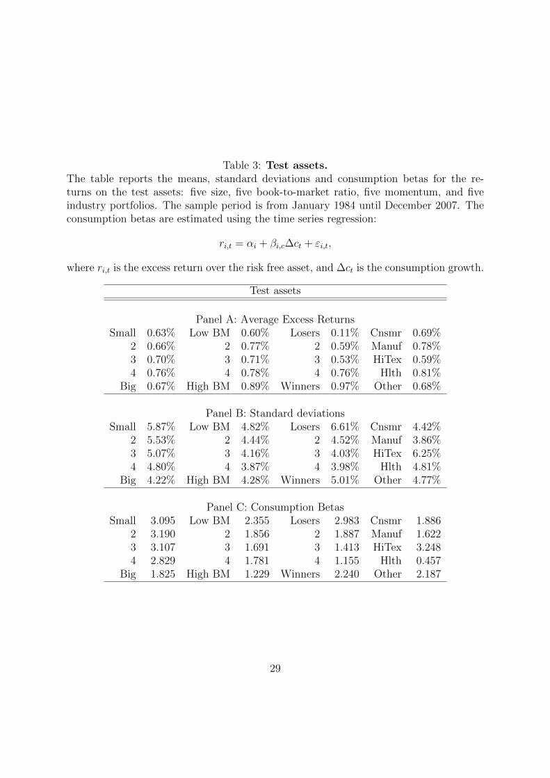
Table 3: Test assets.The table reports the means, standard deviations and consumption betas for the re-turns on the test assets: five size, five book-to-market ratio, five momentum, and fiveindustry portfolios. The sample period is from January 1984 until December 2007. Theconsumption betas are estimated using the time series regression:

ri,t = αi + βi,c∆ct + εi,t,

where ri,t is the excess return over the risk free asset, and ∆ct is the consumption growth.

Test assets

Panel A: Average Excess ReturnsSmall 0.63% Low BM 0.60% Losers 0.11% Cnsmr 0.69%

2 0.66% 2 0.77% 2 0.59% Manuf 0.78%3 0.70% 3 0.71% 3 0.53% HiTex 0.59%4 0.76% 4 0.78% 4 0.76% Hlth 0.81%

Big 0.67% High BM 0.89% Winners 0.97% Other 0.68%

Panel B: Standard deviationsSmall 5.87% Low BM 4.82% Losers 6.61% Cnsmr 4.42%

2 5.53% 2 4.44% 2 4.52% Manuf 3.86%3 5.07% 3 4.16% 3 4.03% HiTex 6.25%4 4.80% 4 3.87% 4 3.98% Hlth 4.81%

Big 4.22% High BM 4.28% Winners 5.01% Other 4.77%

Panel C: Consumption BetasSmall 3.095 Low BM 2.355 Losers 2.983 Cnsmr 1.886

2 3.190 2 1.856 2 1.887 Manuf 1.6223 3.107 3 1.691 3 1.413 HiTex 3.2484 2.829 4 1.781 4 1.155 Hlth 0.457

Big 1.825 High BM 1.229 Winners 2.240 Other 2.187

29

Table 4: Consumption tracking portfolios.The table reports the descriptive statistics for our consumption tracking portfolios. Thesample period is from January 1984 until December 2007. We estimate each CTP byseparate linear regression of consumption growth on each set of base assets: stocks,bonds, and commodity futures returns. We report the values for the tracking portfolioswith fixed weights estimated in the unconditional (CTPc, CTPs, CTPb) and conditional(CTPc,c, CTPs,c, CTPb,c) setup. Panel A shows means and standard deviations forconsumption growth and consumption tracking portfolios and below we report R2s andp-values for the joint significance of the regression coefficients from the regressions usedto create tracking portfolios. Panel B shows the correlation matrix for different trackingportfolios and Panel C gives the estimated weights of each base asset in the trackingportfolios.

Consumption Tracking Portfolios

Panel A: Descriptive statisticsCG CTPc CTPs CTPb CTPc,c CTPs,c CTPb,c

mean 0.16% 0.16% 0.16% 0.16% 0.12% 0.11% 0.12%std 0.29% 0.08% 0.09% 0.06% 0.08% 0.09% 0.06%R2 8.88% 9.97% 3.8% 14.03% 13.06% 7.76%p 0.08 0.03 0.64 0.01 0.03 0.17

Panel B: correlation matrixCG CTPc CTPs CTPb CG CTPc,c CTPs,c CTPb,c

CG 1 CG 1CTPc 0.285 1 CTPc,c 0.278 1CTPs 0.316 0.128 1 CTPs,c 0.309 0.104 1CTPb 0.195 0.193 0.212 1 CTPb,c 0.188 0.201 0.146 1

30

Tab

le4

ctd.:

Consu

mpti

on

track

ing

port

foli

os

ctd.

Pan

elC

:C

oeffi

cien

tson

the

bas

eas

sets

CT

Pc

CT

Pc,

cC

TP

sC

TP

s,c

CT

Pb

CT

Pb,c

Coef

.SE

Coef

.SE

Coef

.SE

Coef

.SE

Coef

.SE

Coef

.SE

const

ant

0.00

10.

000

0.00

20.

001

const

ant

0.00

20.

000

0.00

10.

001

const

ant

0.00

20.

000

0.00

10.

001

Ener

gy(r

1)0.

042

0.02

50.

033

0.02

4In

dex

-0.0

050.

007

-0.0

050.

007

TB

Shor

t-0

.047

0.11

4-0

.060

0.11

6M

eats

(r1)

-0.0

030.

014

-0.0

040.

014

Food

-0.0

070.

003

-0.0

060.

003

TB

Int

-0.0

470.

064

-0.0

670.

066

Met

als

(r1)

0.00

70.

007

0.00

60.

007

Min

es0.

003

0.00

50.

002

0.00

5A

AA

Int

-0.0

240.

099

-0.0

080.

099

Agr

(r1)

0.04

50.

030

0.05

20.

030

Oil

0.00

30.

007

0.00

10.

007

AA

ALT

0.10

60.

057

0.12

20.

057

Ener

gy(r

2)-0

.026

0.06

4-0

.021

0.06

3C

lths

-0.0

090.

007

-0.0

090.

007

AA

Int

0.03

60.

132

0.07

10.

133

Mea

ts(r

2)0.

007

0.01

80.

007

0.01

8D

urb

l0.

003

0.00

70.

006

0.00

7A

ALT

0.01

80.

071

0.02

30.

071

Met

als

(r2)

0.00

30.

067

0.02

00.

066

Chem

s-0

.009

0.00

6-0

.008

0.00

6A

Int

0.04

00.

121

0.04

00.

121

Agr

(r2)

-0.1

160.

047

-0.1

250.

048

Cnsu

m0.

012

0.00

60.

011

0.00

7A

LT

-0.0

830.

078

-0.1

100.

079

Ener

gy(r

3)-0

.136

0.09

0-0

.104

0.08

9C

nst

r0.

005

0.00

50.

006

0.00

5B

AA

Int

-0.0

260.

075

-0.0

430.

075

Mea

ts(r

3)0.

009

0.03

10.

010

0.03

1Ste

el-0

.004

0.00

8-0

.002

0.00

8B

AA

LT

-0.0

110.

057

-0.0

040.

057

Met

als

(r3)

-0.0

090.

164

-0.0

240.

162

Fab

Pr

-0.0

020.

005

-0.0

010.

005

Junk

Int

0.01

80.

021

0.01

30.

021

Agr

(r3)

0.07

80.

031

0.08

20.

031

Mac

hn

-0.0

100.

005

-0.0

110.

005

Junk

LT

0.00

00.

016

0.00

20.

017

Ener

gy(r

4)0.

148

0.05

70.

115

0.05

6C

ars

0.00

40.

007

0.00

30.

007

TE

RM

0.00

00.

000

Mea

ts(r

4)-0

.024

0.03

7-0

.019

0.03

7T

rans

0.00

00.

006

0.00

10.

006

DE

F-0

.005

0.07

9M

etal

s(r

4)0.

119

0.20

70.

122

0.20

4U

tils

0.00

60.

008

0.00

60.

008

MA

RK

ET

0.00

00.

000

Agr

(r4)

-0.0

210.

018

-0.0

200.

017

Rta

il0.

003

0.00

70.

003

0.00

7D

Y0.

000

0.00

0E

ner

gy(r

5)-0

.025

0.01

4-0

.022

0.01

4F

inan

0.00

40.

009

0.00

60.

009

UI

-0.1

540.

097

Mea

ts(r

5)0.

010

0.01

70.

004

0.01

7O

ther

0.00

50.

007

0.00

00.

008

ESR

0.79

60.

342

Met

als

(r5)

-0.1

230.

118

-0.1

260.

115

TE

RM

0.00

00.

000

EL

R-0

.226

0.71

4A

gr(r

5)0.

015

0.01

00.

013

0.01

0D

EF

-0.0

460.

079

TE

RM

0.00

00.

000

MA

RK

ET

0.00

00.

000

DE

F0.

095

0.04

3D

Y0.

000

0.00

0M

AR

KE

T0.

000

0.00

0U

I-0

.104

0.09

5D

Y0.

000

0.00

0E

SR

0.51

40.

345

UI

-0.0

600.

082

EL

R-0

.208

0.66

3E

SR

0.54

30.

322

EL

R-0

.081

0.62

8

31

Table 5: The CCAPM with unconditional CTP.The table reports in Panel A the average returns and the full-sample consumption betas,βi,c, as well s the betas with respect to the unconditional consumption tracking portfolios,βi,CTP , for the 20 test portfolios. CTPc stands for commodity-based consumption trackingportfolio, CTPs for the stock-based, and CTPb for the bond-based tracking portfolios.Panels B and C report the results of the portfolio-level asset pricing tests. Panel B reportsthe average coefficients and their associated t-statistics from monthly Fama and MacBeth(1973) cross-sectional regressions. In Panel C, we estimate the stochastic discount factorrepresentation of the form

E[(1− b′f) rt] = 0

and report the estimated coefficients, b, with their associated t-statistics, as well as theJ-test for the overidentifying restrictions.

32

Tab

le5

ctd.:

The

CC

AP

Mw

ith

unco

ndit

ional

CT

Pct

d.

Pan

elA

:C

onsu

mpti

onb

etas

Sm

all

23

4B

igL

oser

s2

34

Win

ner

s

R0.

63%

0.66

%0.

70%

0.76

%0.

67%

0.11

%0.

59%

0.53

%0.

76%

0.97

%βi,c

3.09

53.

190

3.10

72.

829

1.82

52.

983

1.88

71.

413

1.15

52.

240

βi,CTPc

4.99

75.

176

5.33

96.

168

4.36

6-0

.238

1.75

92.

705

3.69

88.

718

βi,CTPs

28.6

4229

.701

27.7

4926

.729

19.5

0030

.760

18.4

4415

.655

15.0

0024

.701

βi,CTPb

36.3

4140

.475

38.5

7934

.755

24.1

8442

.206

28.1

6024

.083

22.8

9926

.551

Low

BM

23

4H

igh

BM

Cnsm

rM

anuf

HiT

exH

lth

Oth

er

R0.

60%

0.77

%0.

71%

0.78

%0.

89%

0.69

%0.

78%

0.59

%0.

81%

0.68

%βi,c

2.35

51.

856

1.69

11.

781

1.22

91.

886

1.62

23.

248

0.45

72.

187

βi,CTPc

4.50

04.

271

4.18

04.

869

6.29

03.

869

2.76

75.

387

4.36

55.

974

βi,CTPs

22.9

9619

.348

19.1

4616

.220

15.2

7219

.447

16.0

9031

.847

4.14

322

.178

βi,CTPb

26.8

6631

.130

29.7

1729

.985

30.8

1031

.197

24.0

6529

.184

20.1

4832

.931

Pan

elB

:F

ama-

Mac

Bet

hP

anel

C:

GM

MIn

tC

GC

TP

cC

TP

sC

TP

bR

2/R

2 adj

CG

CT

Pc

CT

Ps

CT

Pb

J/

p

Coef

.0.

87%

-0.0

9%16

.53%

53.9

835

.31

tt3.52

-0.93

11.8

9%0.82

0.01

Coef

.0.

37%

0.07

%57

.93%

893.

4217

.28

t1.33

2.60

55.5

9%3.15

0.57

Coef

.0.

91%

-0.0

1%18

.06%

57.3

037

.17

t3.54

-0.98

13.5

1%0.62

0.01

Coef

.1.

07%

-0.0

1%19

.35%

431.

9033

.09

t3.28

-1.16

14.8

7%2.02

0.02

Coef

.0.

63%

0.07

%0.

00%

0.01

%84

.67%

802.

78-6

7.87

221.

0717

.66

t1.92

2.78

-0.19

0.71

81.8

0%2.60

-0.57

0.83

0.41

33

Table 6: The CCAPM with conditional CTP.The table reports analogous to Table 5 summary of the estimation of the ConsumptionCAPM on a set of 20 portfolio returns as test assets, but using consumption tracking port-folios that are estimated conditionally. Panel A reports the consumption betas estimatedin the time-series regressions. Panel B reports the results for the Fama and MacBeth(1973) cross-sectional regression and Panel C for the GMM estimation of Hansen (1982).See caption of Table for details.

Panel A: Consumption betas

Small 2 3 4 Big Losers 2 3 4 WinnersR 0.63% 0.66% 0.70% 0.76% 0.67% 0.11% 0.59% 0.53% 0.76% 0.97%

βi,CTPc 4.093 4.708 5.184 6.070 4.428 4.361 4.427 4.302 4.790 6.411βi,CTPs 23.807 26.926 26.250 26.126 20.302 23.913 19.280 18.563 15.353 13.868βi,CTPb 24.902 29.922 28.932 25.960 16.793 18.784 23.642 22.522 23.758 22.707

Low BM 2 3 4 High BM Cnsmr Manuf HiTex Hlth OtherR 0.60% 0.77% 0.71% 0.78% 0.89% 0.69% 0.78% 0.59% 0.81% 0.68%

βi,CTPc 0.781 2.134 2.846 3.925 8.264 3.892 3.263 5.468 3.821 5.780βi,CTPs 28.314 17.826 15.595 15.349 24.950 18.768 16.655 32.804 4.869 21.335βi,CTPb 28.022 19.810 17.735 17.148 19.924 23.928 18.904 17.897 14.915 25.055

Panel B: Fama-MacBeth Panel C: GMMInt CTPc CTPs CTPb R2 R2

adj CTPc CTPs CTPb J p

Coef. 0.32% 0.08% 56.78% 54.38% 985.07 15.60 0.68t 1.15 2.77 3.20

Coef. 0.90% -0.01% 15.46% 10.77% 92.96 36.19 0.01t 3.56 -0.95 0.97

Coef. 0.90% -0.01% 5.89% 0.66% 432.26 31.69 0.03t 2.90 -0.75 2.07

Coef. 0.59% 0.09% -0.01% 0.00% 85.06% 82.26% 892.60 -35.79 172.45 16.20 0.51t 1.84 3.01 -1.21 -0.07 2.68 -0.31 0.66

34

Table 7: The firm-level CCAPM.The table reports the time-series average coefficients and their associated t-statisticsfrom the monthly firm-level Fama-MacBeth regressions. The individual stocks’ betas areshrinked to the averages of betas of the stocks from the same industry with similar pre-ranking betas. CTPc stands for commodity-based consumption tracking portfolio, CTPsfor the stock-based, and CTPb for the bond-based tracking portfolios. LnSize is thenatural logarithm of market equity, LnB/M is the natural logarithm of book-to-marketequity, Ret(-1:-1) is the previous month’s return, Ret(-12:-2) is the cumulative returnfrom month -12 to month -2, and Ret(-36:-13) is the cumulative return from month -36to month -13. Panel A reports the results for betas with respect to the unconditionalconsumption tracking portfolios and Panel B reports those for the conditional trackingportfolios.

βCTPc βCTPs βCTPb LnSize LnB/M Ret(-1:-1) Ret(-12:-2) Ret(-36:-13) R2

Panel A: unconditional CTP

Coef. 0.04% 0.14%t 2.10

Coef. 0.01% 1.22%t 0.62

Coef. 0.00% 0.47%t 0.06

Coef. 0.04% 0.01% -0.01% 1.45%t 2.26 0.77 -1.27

Coef. 0.05% -0.09% 0.19% -4.49% 0.36% -0.23% 3.03%t 2.87 -1.50 1.99 -8.61 2.10 -3.94

Coef. 0.01% -0.09% 0.21% -4.65% 0.37% -0.21% 3.61%t 0.93 -1.48 2.59 -9.36 2.33 -3.83

Coef. 0.00% -0.09% 0.18% -4.60% 0.38% -0.23% 3.29%t -0.16 -1.56 1.84 -8.90 2.26 -4.08

Coef. 0.04% 0.01% -0.01% -0.09% 0.21% -4.73% 0.37% -0.20% 3.83%t 2.80 1.28 -1.85 -1.55 2.60 -9.55 2.30 -3.80

Panel B: conditional CTP

Coef. 0.03% 0.07%t 2.06

Coef. 0.01% 1.11%t 0.68

Coef. -0.01% 0.18%t -1.19

Coef. 0.03% 0.01% -0.02% 1.32%t 1.91 0.73 -1.62

Coef. 0.03% -0.09% 0.19% -4.47% 0.36% -0.23% 3.00%t 2.38 -1.53 1.87 -8.56 2.12 -3.95

Coef. 0.01% -0.09% 0.20% -4.63% 0.36% -0.21% 3.57%t 1.11 -1.53 2.46 -9.27 2.30 -3.82

Coef. -0.02% -0.10% 0.18% -4.55% 0.37% -0.23% 3.10%t -1.42 -1.59 1.83 -8.72 2.14 -3.96

Coef. 0.03% 0.02% -0.02% -0.09% 0.21% -4.70% 0.36% -0.20% 3.75%t 2.06 1.24 -2.05 -1.56 2.58 -9.48 2.28 -3.73

35

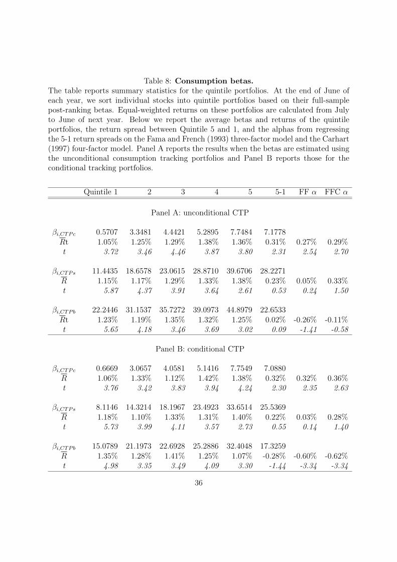
Table 8: Consumption betas.The table reports summary statistics for the quintile portfolios. At the end of June ofeach year, we sort individual stocks into quintile portfolios based on their full-samplepost-ranking betas. Equal-weighted returns on these portfolios are calculated from Julyto June of next year. Below we report the average betas and returns of the quintileportfolios, the return spread between Quintile 5 and 1, and the alphas from regressingthe 5-1 return spreads on the Fama and French (1993) three-factor model and the Carhart(1997) four-factor model. Panel A reports the results when the betas are estimated usingthe unconditional consumption tracking portfolios and Panel B reports those for theconditional tracking portfolios.

Quintile 1 2 3 4 5 5-1 FF α FFC α

Panel A: unconditional CTP

βi,CTPc 0.5707 3.3481 4.4421 5.2895 7.7484 7.1778Rt 1.05% 1.25% 1.29% 1.38% 1.36% 0.31% 0.27% 0.29%t 3.72 3.46 4.46 3.87 3.80 2.31 2.54 2.70

βi,CTPs 11.4435 18.6578 23.0615 28.8710 39.6706 28.2271R 1.15% 1.17% 1.29% 1.33% 1.38% 0.23% 0.05% 0.33%t 5.87 4.37 3.91 3.64 2.61 0.53 0.24 1.50

βi,CTPb 22.2446 31.1537 35.7272 39.0973 44.8979 22.6533Rt 1.23% 1.19% 1.35% 1.32% 1.25% 0.02% -0.26% -0.11%t 5.65 4.18 3.46 3.69 3.02 0.09 -1.41 -0.58

Panel B: conditional CTP

βi,CTPc 0.6669 3.0657 4.0581 5.1416 7.7549 7.0880R 1.06% 1.33% 1.12% 1.42% 1.38% 0.32% 0.32% 0.36%t 3.76 3.42 3.83 3.94 4.24 2.30 2.35 2.63

βi,CTPs 8.1146 14.3214 18.1967 23.4923 33.6514 25.5369R 1.18% 1.10% 1.33% 1.31% 1.40% 0.22% 0.03% 0.28%t 5.73 3.99 4.11 3.57 2.73 0.55 0.14 1.40

βi,CTPb 15.0789 21.1973 22.6928 25.2886 32.4048 17.3259R 1.35% 1.28% 1.41% 1.25% 1.07% -0.28% -0.60% -0.62%t 4.98 3.35 3.49 4.09 3.30 -1.44 -3.34 -3.34

36

Table 9: The CCAPM with commodity index.The table reports the estimates of the Consumption CAPM when using an equallyweighted index of commodity futures returns instead of consumption tracking portfo-lio. Panel A reports the results for the Fama-MacBeth (1973) cross-sectional regressionand the GMM estimation of Hansen (1982) for the 20 stock portfolios. Panel B reportsthe results for the firm-level regressions. We report coefficient estimates and the corre-sponding t-statistics, as well as the cross-sectional R2s for the Fama-MacBeth regressionsand the J-test for the overidentifying restrictions with the corresponding p-value for theGMM tests. See captions of Table 5 and 7 for details.

Panel A: Portfolio level resultsFama-MacBeth GMM

EW com R2 R2-adj EW com J p

Coef. -0.22% 2.07% -3.37% 1.45 36.86 0.01t -0.43 0.39

Panel B: Firm-level regressionsEW com LnSize LnB/M Ret(-1:-1) Ret(-12:-2) Ret(-36:-13) R2

Coef. 0.34% 0.62%t 1.09

Coef. 0.27% -0.09% 0.18% -4.55% 0.35% -0.22% 3.43%t 0.96 -1.57 1.86 -8.73 2.08 -3.89

37

Fig

ure

1:R

eali

zed

vers

us

Fit

ted

Exce

ssR

etu

rns.

38