EDHEC RISK AND ASSET MANAGEMENT RESEARCH CENTRE EDHEC - 393-400 promenade des Anglais, 06202 Nice - Tel. +33 (0)4 93 18 78 24 - Fax. +33 (0)04 93 18 78 44

Email: research@edhec-risk.com – Web: www.edhec-risk.com

Commodities – Active Strategies for Enhanced Return

Hilary Till

Co-founder of Premia Capital Management, LLC Research Associate with the EDHEC Risk and Asset Management Research Centre

Till@premiacap.com

Joseph Eagleye

Co-founder of Premia Capital Management, LLC Eagleeye@premiacap.com

November 2005

2

Abstract In this article, we note how a set of active commodity strategies could potentially add value to an investor’s commodity

allocation. But we also emphasize the due care that must be taken in risk management and implementation discipline,

given the “violence of the fluctuations which normally affect the prices of many … commodities,” as Keynes (1934)

put it. We take it as a given that a prudent investor should include commodities in their overall asset allocation mix. As

Greer of Pimco (2005) has noted, the benefits of commodity indexes include positive correlation to inflation as well as

positive correlation to changes in the rate of inflation. Commodity indexes can also potentially perform well during a

number of adverse economic surprises that are harmful to investments in stocks and bonds.

Authors’ Note: A version of this article appeared in the Journal of Wealth Management, Fall 2005 edition; and as a

chapter in the edited book, The Handbook of Inflation Hedging Investments (Edited by Robert Greer), McGraw Hill,

2006.

EDHEC is one of the top five business schools in France owing to the high quality of its academic staff (100 permanent lecturers from France and abroad) and its privileged relationship with professionals that the school has been developing since its establishment in 1906. EDHEC Business School has decided to draw on its extensive knowledge of the professional environment and has therefore concentrated its research on themes that satisfy the needs of professionals. EDHEC pursues an active research policy in the field of finance. Its “Risk and Asset Management Research Centre” carries out numerous research programs in the areas of asset allocation and risk management in both the traditional and alternative investment universes.

Copyright © 2006 EDHEC

3

In this article, we note how a set of active commodity strategies could potentially add value to an investor’s commodity allocation. But we also emphasize the due care that must be taken in risk management and implementation discipline, given the “violence of the fluctuations which normally affect the prices of many … commodities,” as Keynes (1934) put it. We take it as a given that a prudent investor should include commodities in their overall asset allocation mix. As Greer of Pimco (2005) has noted, the benefits of commodity indexes include positive correlation to inflation as well as positive correlation to changes in the rate of inflation. Commodity indexes can also potentially perform well during a number of adverse economic surprises that are harmful to investments in stocks and bonds. THE ROLE OF ACTIVELY MANAGED COMMODITY STRATEGIES We would argue that the role of active commodity strategies is as a satellite to an investor’s core exposure to commodities, which in turn should be obtained through commodity index investments. With commodity indexes, an investor obtains consistent exposure to the inherent returns of the asset class. In an actively managed commodity hedge fund, there is no guarantee that a manager will remain consistently long of commodities. As a matter of fact, it is a core risk management principle for most hedge funds that total risk should be managed by neutralizing systematic risk through hedging. An idealized hedge fund is not supposed to deliver a consistent beta; it is supposed to either deliver pure alpha (if it is a relative-value fund) or well-timed beta exposures (if it is a global macro fund.) If an investor’s long-term asset allocation plan were designed around the expectation that its commodity allocation would provide protection against say an oil shock, the plan’s purpose could be compromised if it were exclusively invested in actively managed commodity programs. For example, prior to the first Gulf War, an active commodity program might have excluded long positions in oil since at the time, the term structure of that futures market indicated surplus. If an investor’s commodity exposure were solely with such a program, then that investor would have missed out on having an oil dislocation hedge just when this portfolio protection was needed the most.

4

THE BENEFITS AND LIMITATIONS OF ACTIVELY MANAGED COMMODITY STRATEGIES Once an investor has obtained their core commodity exposure through a commodity index investment, the next logical step is to include active commodity managers for further value-added. This is analogous to the evolving nature of equity management whereby active management is being unbundled from passive index investments. A number of investors are now getting core equity exposure through equity index funds, exchange-traded funds, and/or futures and then investing in long/short equity hedge funds for further value-added. Benefits To demonstrate the benefits of active commodity management, Akey of Cole Partners (2005) created a comprehensive database of known active commodity futures traders. These traders identified themselves as focusing exclusively on non-financial commodity markets. Akey then created an equally-weighted portfolio of both active and inactive programs from this database. By including inactive programs, the author attempted to limit survivorship bias. Exhibit 1 shows the return and risk statistics for an equally-weighted portfolio of active commodity futures traders from January 1991 through November 2004.

Exhibit 1

Active Commodity Futures Traders Returns (January 1991 through November 2004)

Compound Annualized Sharpe Worst Annual Return Standard Deviation Ratio Draw-Down

20.99% 10.48% 1.63 -8.49% Data Source: Excerpted from Akey (2005), Figure 19. These results suggest that an investor may be able to source skilled commodity managers who can achieve superior returns with acceptable risk. Akey also provided evidence that the active manager returns were likely not related to commodity index exposure. Exhibit 2 shows how low the empirical correlations of the active portfolio were with various commodity indices. This is a reassuring property for an investor since under the core-satellite approach to portfolio management, an investor should be obtaining their core commodity exposure through cost-effective index products rather than through expensive active managers. The role of active managers is then to provide uncorrelated returns over those of the investor’s commodity index investments.

5

Exhibit 2

Correlation of Monthly Returns Active Commodity Futures Traders vs. Passive Indices

(January 1991 through November 2004)

CRBR DJAIG Active Portfolio GSCI RICI SPCICRBR 1.00DJAIG 0.82 1.00Active Portfolio 0.25 0.26 1.00GSCI 0.65 0.89 0.18 1.00RICI 0.72 0.90 0.25 0.92 1.00SPCI 0.81 0.91 0.22 0.87 0.82 1.00 Abbreviations: CRBR: Commodities Research Bureau – Reuters Total Return Index; DJAIG: Dow Jones – AIG Commodity Index; GSCI Goldman Sachs Commodity Index; RICI: Rogers International Commodity Index; and SPCI: Standard and Poor’s Commodity Index. Data Source: Akey (2005), Figure 22. Limitations The main limitation of active commodity strategies is scalability, which arises from two sources. First, one can argue that all hedge fund strategies, which exploit inefficiencies, are by definition capacity-constrained. If hedge funds are exploiting inefficiencies, this means that other investors are supplying those inefficiencies. And unfortunately, we can’t all profit from exploiting inefficiencies since in that case, nobody would be supplying inefficiencies. In Till (2004), we argue that a plausible maximum size of the hedge fund industry is 6% of institutional and high net worth assets. A second factor that limits the size of active commodity strategies is unique to the futures markets. Unlike investors in the securities markets, traders of futures contracts in certain markets may not exceed the speculative position limits (spec limits) set for those markets. Spec limits impose a cap on the size of the net position that speculators may hold overnight in a single contract month and in all contract months of a particular commodity. Often, this cap is even more restrictive in the spot month.

6

The Commodity Futures Trading Commission (CFTC) sets the spec limits for the grains and cotton. The commodity exchanges, with the Commission’s approval, set the limits for all other markets. The purpose of spec limits is to prevent a trader from amassing a large position that he (or she) could use to manipulate futures prices. According to Gillman (2005), the Commission routinely reexamines the utility of spec limits in different markets. For example, in the 1990’s, it approved exchange rules adopting “trader accountability exemptions,” which give more flexibility to traders in the largest and most liquid markets. For many of these large traders, spec limits have proven less of a burden than one might expect. This is because the size of spec limits is tied closely to market liquidity, and many large traders carefully limit positions in illiquid markets or avoid these markets entirely. In the future, though, active commodity futures trading strategies may face new capacity challenges. During times of commodity market stress, it is not unusual to read of proposals for futures exchanges to “tighten position limits on traders,” as discussed in Verleger (2005). For example, in early 2005, “The Consumers Alliance for Affordable Natural Gas … recommended that the Commodity Futures Trading Commission report to Congress if the number of [natural gas] contracts a single entity can own results in a concentration that may distort the market,” according to a news bulletin quoted by Verleger. One way that active commodity managers can potentially increase the capacity of their strategies is to move their transactions off of futures exchanges and over to the over-the-counter (OTC) swap markets. This may be occurring now. According to Lammey (2005), “because of the controversy over the impact and influence of hedge funds in the [energy] market, some sources report that hedge funds have been quietly … [using] brokerage companies to … [enter into] complex combinations of futures, options, and other derivatives.” Further, “funds have found that trading via the brokerage firms provides greater liquidity than at the NYMEX [the energy futures exchange] and reduces the chance that they will find themselves accidentally taking delivery of actual crude oil or gas. Additionally … brokerage firms often allow big funds to make trades with favorable financing terms and trade with more leverage than on an exchange.” If an active commodity manager uses private transactions to gain exposure to the commodity markets, then the manager’s clients must be willing to assume the attendant credit risk of the OTC counterparties used in these transactions. In summing up this section, we would say that while an examination of the universe of commodity futures traders reveals that there are skillful active commodity funds, which an investor can potentially invest in, the commodity markets present unique capacity problems, which can be even more challenging than for hedge fund strategies that focus on the financial markets.

7

SOURCES OF STRUCTURAL RETURN In this section, we discuss persistent sources of return in the commodity futures markets. A later section of the article will then discuss how to design an investment process around these sources of return. The key to understanding why there should be structural returns in the commodity futures markets is to realize that futures markets are not zero-sum games. As noted in Di Tomasso and Till (2000), when one only focuses on the narrow realm of commodity futures markets, it is obvious that for every winner there must be a loser. But this simplifies away the fact that each commodity futures market is embedded within a wider scheme of profits, losses, and risks of its physical commodity market. Commodity futures markets exist to facilitate the transfer of exceptionally expensive inventory risk. Moreover, commodity futures markets allow producers, merchandisers, and marketers the benefit of laying off inventory price risk at their timing and convenience. For this, commercial participants will tolerate paying a premium so long as this cost does not overwhelm the overall profits of their business enterprise, as discussed in Working (1948). Further, Cootner (1967) documents price pressure effects resulting from commercial hedging in a number of agricultural futures markets and notes that these effects are well known by commercial market participants. He concludes that the fact that these effects “persist in the face of such knowledge indicates that the risks involved in taking advantage of them outweigh the gain involved. This is further evidence that the trade does not act on the basis of expected values; that it is willing to pay premiums to avoid risk.” Hedge Pressure In this section, we will review both the hypothesis and evidence that there is a persistent return from taking a position on the other side of commercial hedge pressure. In certain commodity futures markets, there tends to be an excess of commercial entities that are short hedgers. Therefore, in order to balance the market, investors must be willing to take up the slack of the long side of these markets. And in order to be persuaded to enter these markets, investors need a return for their risk-bearing. “In effect the hedgers offer … [investors] an insurance premium for this service,” as Bodie and Rosansky (1980) put it. In other words, investors can earn an “insurance premium” for being long certain commodity futures contracts. (For example, Greer (2005) discusses how investors can earn an insurance premium in the cattle futures markets.) Hicks (1939) explains that “in all forward markets there is likely to be a tendency for hedgers to predominate on one side or the other over long periods. No forward market can do without the speculative element.” Further, in some commodity futures markets,

8

producers are in a more vulnerable position than consumers and so will be under more pressure to hedge than consumers. This leads to a “congenital weakness” on the demand side for some commodity futures contracts, which causes these contracts’ futures prices to be downwardly biased relative to future spot prices, which in turn leads to generally positive returns for holding the futures contract. Live cattle and gasoline are examples of two commodity futures markets where there appears to be a systematic positive return due to a “congenital weakness” on the demand side for hedging. Live Cattle Helmuth (1981) reports that the “amount of short hedging in the live cattle futures market is almost four times as large as the amount of long hedging. Long hedging as a percent of open interest averages about 8 percent while short hedging averages over 30 percent. Thus, unlike grain futures, in live cattle futures there is no significant group of commercial long hedgers who act as a buying force without significant regard to price level. There is very little long hedging because meat is not sold on long-term, fixed-price forward contracts.” Gasoline Verleger (2005) explains that “the gasoline business has for years lacked a natural long to offset the natural short position of refiners and traders. … The absence of natural longs is explained by the retail nature of retail gasoline sales. Consumers buy product in very modest amounts – 50 gallons at most – at any one time. Consumers generally do not frequent the same supplier for all their purchases, and prices vary widely by location. The random feature of the purchase decision combined with the dispersion of retail prices makes it almost impossible for most buyers to hedge.”1 The most convincing evidence of there being a systematic downward bias in the prices of live cattle and gasoline futures prices comes from directly examining their long-term returns. Nash and Shrayer of Morgan Stanley (2004) report that the annualized returns for live cattle and gasoline have been 11.0% and 18.6% respectively over twenty-year-plus timeframes. Both calculations include the interest income from fully collateralizing positions in these two futures markets. The horizon over which the live cattle returns were calculated was from April 1983 to April 2004. For gasoline, the horizon was from January 1985 to April 2004. Grain Markets For the grain markets, there have historically been seasonal times when commercial hedging tends to be long rather than short. Therefore, one might expect that in order to

1 Verleger (2005) notes, though, that with increased investor participation in the commodity markets, the dynamics of the gasoline futures markets might change. That said, he notes that open interest in the summer gasoline futures contracts currently “only covers ten percent of demand.”

9

capture the gains from being on the other side of commercial hedge pressure, there are times when an investor’s positioning needs to be from the short side rather than from the long side. In other words, when commercial hedgers are net long, we would expect that the corresponding futures price would have a tendency to be biased upwards, leading to systematic profits for an investor taking a short position in the contract. Conversely, when commercial hedgers are net short, we would expect the corresponding futures price would have a tendency to be biased downwards, leading to systematic profits for an investor taking a long position in the contract. Bessembinder (1992) provided empirical evidence that this is the proper way to approach the grain markets. He obtained net hedging data from the CFTC’s Commitment of Traders (COT) report. In this way, he could identify periods when hedgers were net long versus net short. Using data from 1967 to 1989, he examined what the average returns were for twenty-two futures markets, conditioned on whether hedgers were net short or net long. Exhibit 3 summarizes his results for soybeans, wheat, and corn.

Exhibit 3 Mean returns (% per day * 250) in Selected Futures Markets

Conditional on net hedging

Short Long

Soybeans 4.35% -1.21%

Wheat 5.71% -10.53%

Corn 16.25% -19.96%

Source: Excerpted from Bessembinder (1992), Table 1. Maddala and Yoo (1990) confirmed the thrust of Bessembinder’s study using both futures price and COT data from 1976 to 1984. The futures markets that they studied included wheat, corn, oats, soybeans, soybean oil, and soybean meal. The researchers calculated the monthly rate of return to both larger hedgers and large speculators as a whole. They found that “large hedgers consistently lose money on … average … [while] large speculators consistently make money on … average.” In the case of the grain markets, it appears that “future prices are biased against both long and short hedgers,” quoting Cootner (1967).

10

Spread Markets Price pressure effects due to commercial hedging can be detected in futures spreads as well. Certain commodity futures spreads represent processing margins. Examples include the gasoline crack spread, which is the differential between gasoline futures prices and crude oil futures prices, and the soybean crush spread, which is the differential between soybean product prices and soybean futures prices. There are times when commercial entities lock in processing margins via the futures markets, which appears to exert one-sided pressure on these spreads. Again, on average a commodity investor earns a return by taking the other side of these transactions. Girma and Paulson (1998) provide empirical evidence of this price-pressure effect for a number of petroleum futures spreads. For heating oil vs. crude oil futures spreads, the horizon of Girma and Paulson’s study is over the period, April 1983 through December 1994. For gasoline vs. crude oil futures spreads, the horizon is over the period, December 1984 through December 1994. Scarcity Another source of return in the commodity futures markets results from buying commodities when they are scarce. This sounds as simple as saying that a source of return in the stock market results from buying equities when they are cheap. The complications arise when one needs to define the technical indicator for when commodities are scarce or when equities are cheap. For example, Asness et al. (2000) describe some fairly involved calculations to come up with a basket of value stocks; their technical indicator for value stocks goes beyond merely examining stocks with high book-to-price ratios. In the case of commodities, we will use a futures curve’s term structure to indicate whether a commodity is scarce or not. By term structure, we mean one should examine the relative price differences of a futures contract across delivery months. When a near-month contract is trading at a premium to more distant contracts, we say that a commodity futures curve is in “backwardation.” Conversely, when a near-month contract is trading at a discount to more distant contracts, we say that the curve is in “contango.”

11

Exhibit 4 illustrates the copper futures curve as of the end of March 2005. The graph shows the relative prices of twelve copper futures contracts of varying maturity. Note that at this time we can say that copper is in backwardation.

Exhibit 4

COMEX Copper Futures Curve as of 3/30/05 Price vs. Contract Maturity

135.0

137.0

139.0

141.0

143.0

145.0

147.0

149.0

151.0

Apr-

05

May

-05

Jun-

05

Jul-0

5

Aug-

05

Sep-

05

Oct

-05

Nov

-05

Dec

-05

Jan-

06

Feb-

06

Mar

-06

Futures Maturity

Futu

res

Pric

e

Data Source: Bloomberg. As explained in Till (October 2000), in a normal futures market (i.e. a market in contango), the maximum price difference between the front and back contracts tends to be determined by carrying charges, which include storage costs, insurance, and interest. Backwardation occurs when supplies of commodities are inadequate; therefore, market participants are willing to pay a premium to buy the immediately deliverable commodity. This is precisely the time an active commodity manager should be long a particular futures market: when scarcity is indicated. Since backwardation indicates scarcity, one is on the correct side of a potential price spike in the commodity by being long at that time. Further, backwardation provides a signal that there is not an excess of commodity inventories. The markets abhor an excess of commodity inventories, according to Keynes (1934), because of the enormous expense of financing them. If such excess inventories come into existence, “the price of the goods continues to fall until either consumption increases or production falls off sufficiently to absorb them.”

12

Keynes wrote that our “present economic arrangements make no normal provision for looking after surplus” commodity inventories; this is arguably still true in 2005. Regarding the petroleum complex, Rowland (1997) explains, “from wellheads around the globe to burner tips, the world’s oil stocks tie up enormous amounts of oil and capital. The volume of oil has been estimated at some 7-to 8-billion barrels of inventory, which is the equivalent of over 100 days of global oil output or 2½ years of production from Saudi Arabia, the world’s largest producer and exporter of crude oil. Even at today’s low interest rates, annual financial carrying costs tied up in holding these stocks amount to around $10-billion, which is more than the entire net income of the Royal Dutch/Shell Group, the largest private oil company in the world.” By going long commodities when scarcity is indicated, one would be attempting to avoid being on the wrong side of the “strong forces [that] are immediately brought into play to dissipate” surplus inventories, again quoting Keynes (1934). A number of authors have confirmed that backwardation has historically provided an effective signal for profitably going long certain commodities over lengthy timeframes. For example, Abken (1989) showed that going long heating oil calendar spreads during the times of the year when heating oil tends to trade in backwardation had yielded statistically significant profits from January 1980 through December 1987. A calendar spread consists of taking offsetting positions during different delivery months of a particular futures contract. A long calendar spread consists of taking a long position in a near-month futures contract while simultaneously taking a short position in a deferred-month futures contract. Humphreys and Shimko (1995) described a strategy whereby one invests in energy futures contracts according to which contracts are in backwardation and to what degree they are in backwardation. They find that such a strategy would have earned 20.3% per year in excess of T-bills from 1984 through 1994. More recently Erb and Campbell (2005) showed how one could have historically earned superior returns when investing in the Goldman Sachs Commodity Index (GSCI) by tactically investing in the GSCI only when its futures curve was in backwardation. Their study was over the period, July 1992 to May 2004. Weather Fear Premia Another source of systematic returns in the futures markets are due to “weather premia.” As discussed in Di Tomasso and Till (2000), a futures price will sometimes embed a fear premium due to upcoming, meaningful weather events that can dramatically impact the supply or demand of a commodity. In this class of trades, a futures price is systematically too high, reflecting the uncertainty of an upcoming weather event. We say the price is too high when an analysis of historical data shows that one can make statistically significant profits from being short the commodity futures contract during the relevant time period. And further that the systematic profits from the strategy are sufficiently high that they compensate for the

13

infrequent large losses that occur when the feared, extreme weather event does in fact occur. Till (September 2000) provides examples of weather-fear premia in the grain, tropical, and natural gas futures markets. Here, we provide an example from the coffee futures market. The uncertainty of weather in Brazil appears to create a built-in weather premium in coffee futures prices during certain times of the year. As Teweles and Jones (1987) note, “because of Brazil’s significance as a producer, its susceptibility to frosts and droughts, and its April-to-August harvesting season, the June-July period is subject to volatile, uncertain price movements [in coffee futures prices].” According to historical data from 1980 to 2004, coffee futures prices have declined coming into the Brazilian winter, consistent with the market getting comfortable with taking some weather premium out of the futures price. Of note is that the exit date for this weather-premium study is before the actual onset of Brazilian winter. Exhibit 5 illustrates the risk of a short position in coffee if such a position is held during the Southern Hemisphere winter; in 1994 consecutive bouts of extreme weather did occur, as described in Cordier (2005).

Exhibit 5

Coffee Futures Price (KCN94)

70

90

110

130

150

170

190

210

230

250

4/4/199

4

4/11/1

994

4/18/1

994

4/25/1

994

5/2/199

4

5/9/199

4

5/16/1

994

5/23/1

994

5/30/1

994

6/6/199

4

6/13/1

994

6/20/1

994

6/27/1

994

7/4/199

4

7/11/1

994

7/18/1

994

Date

Pric

e (c

ents

per

pou

nd)

Data Source: Bloomberg

14

Caveat on Sources of Structural Return: Past Performance is No Guarantee of Future Success One concern in identifying obscure strategies to monetize risk premia is that by their very identification, one will popularize these strategies to a sufficient degree that future returns may be dampened or even eliminated. For example, Siegel (2003) pointed out that “high-beta stocks beat low-beta stocks until William Sharpe discovered beta in 1964; [and] small stocks beat large ones until Banz and Reinganum discovered the size effect in 1979.” Further, Rosenberg et al. (1985) described how one could have earned abnormal returns in the stock market by buying stocks with a high ratio of book value of common equity per share to market price and selling stocks with a low book/price ratio. The authors’ study was over the horizon, January 1973 through September 1984. The authors said, “we felt that book/price ratio was an intriguing candidate for study. Since it had not been heavily described in the quantitative literature, it might possibly serve as an as-yet unspoiled instrument.” Fourteen years later, Cochrane (1999) wrote that “the size and book/market premia [in the equity markets] seem to have diminished substantially in recent years. If this is permanent, it suggests that these opportunities were simply overlooked.” (Italics added.) As a counter-example, one can also point to other market “inefficiencies” that have been published and yet continue to exist. For example, in 1939 J.R. Hicks developed the widely known “liquidity premium” hypothesis for bonds. In this hypothesis, Hicks (1939) notes that all things being equal, a lender would rather lend in short maturities since they are less volatile than longer-term-maturity bonds. On the other hand, an entrepreneur would rather borrow in a long maturity in order to fix his costs and better plan for the future. In order to induce borrowers to lend long, they must be offered a “liquidity premium” to do so. The result is that bond yield curves tend to be upwardly sloping. Like the hedging pressure hypothesis for certain commodity futures contracts, the central idea behind the “liquidity premium” hypothesis is that commercial entities are willing to pay premiums from the profits of their ongoing businesses in order to hedge away key volatile price risks. Hicks’ identification of there being a liquidity premium in long-maturity bonds has not prevented the U.S. yield curve from continuing to be persistently steep nor has it prevented both mutual funds and hedge funds from designing profitable trading strategies that monetize this premium. Regarding weather-fear premia strategies, these risk premia could obviously be reduced if improvements in forecasting reduced weather uncertainty. It does not appear though that weather forecasting has improved sufficiently just yet to reduce the uncertainty surrounding key weather times.

15

While weather uncertainty should remain a fundamental factor in commodity trading, there is another way that these strategies can become obsolete. For decades the United States had been the dominant soybean producer. It is now the case that Latin American countries produce over 52% of the world’s soybeans, according to Cronin (2003), which means that trading strategies, which focus on U.S. weather, no longer have the potency they once had in the past. Also, to the extent that Vietnam becomes a more significant coffee producer, one may see coffee futures strategies that are timed around Brazilian weather events lose their potency as well. In summing up this section, we would say that while a number of superior investment strategies have historically been quite fleeting, especially once they are popularized, one should add the following about the commodity strategies discussed here. We have discussed persistent sources of return in the commodity futures markets that were originally published between 1967 and 2000, and each of these strategies continues to exist in some form as of 2005. A Note on Commodity Trading Advisors (CTA’s) and Technical Trading Rules Most traders who are known as Commodity Trading Advisors (CTA’s) do not primarily trade natural-resource commodity futures contracts. Instead, they primarily trade financial futures contracts such as currency, interest rate, and equity futures contracts. CTA’s are also known as “managed futures” traders. The dominant trading style employed by managed futures traders is medium-to-long-term systematic trend-following. Exhibit 6 shows that trend-following strategies in currencies, interest rates, and stocks have had the strongest statistical significance in explaining the returns of an index of managed futures traders.

16

Exhibit 6 Regression of Managed Futures Returns on Passive Indices and Economic Variables

(1996-2000)

Coefficient Standard Error T-StatisticIntercept 0.00 0.00 0.01S&P 500 0.00 0.07 0.05Lehman US 0.29 0.39 0.76Change in Credit Spread 0.00 0.01 0.30Change in Term Spread 0.00 0.00 0.18CISDM/Interest Rates 1.27 0.24 5.24CISDM/Currency 1.37 0.25 5.48CISDM/Commodity 0.27 0.15 1.79CISDM/Stock 0.36 0.11 3.17

R-Squared 0.70 The CISDM indexes in this figure are based on passive strategies that replicate CTA strategies in Interest Rates, Currencies, Commodities, and Stocks. Source: Center for International Securities and Derivatives Markets (CISDM) 2nd Annual Chicago Research Conference, 5/22/02, Slide 48. This is not to say that trend-following strategies cannot be profitably employed in the commodity markets. If there are inadequate inventories for a commodity, only its price can respond to equilibrate supply and demand, given that in the short run, new supplies of physical commodities cannot be mined, grown, and/or drilled. When there is a supply/usage imbalance in a commodity market, the price trend may be persistent, which, in turn, systematic trend-following systems may be able to capture. Researchers at Calyon Financial provide evidence that trend-following systems may be able to capture returns in the commodity futures markets. In Burghardt et al. (2004), the researchers create generic trend-following models based on two popular systems, the “moving average/crossover” model and the “range breakout” model. “Each [model] defines a trend or price pattern by comparing a current market price or recent average price with a longer history of the price and buys or sells when the recent price measure is above or below the longer price measure.” While the Calyon research describes employing their technical models to the equity, fixed income, currency, and commodities futures markets, we will just focus on their results for the commodity sector. The commodity futures markets which are included in their simulations are as follows: crude oil, natural gas, sugar, heating oil, cotton, corn, coffee, soybeans, gold, and copper. Duncan (2005) notes that in only reporting Calyon’s commodity results, we are showing unconstrained results. In practice, a managed futures

17

program would include constraints on the sizing of commodity positions that take into consideration the liquidity of these markets. The Calyon study sizes individual futures markets according to their historical standard deviations in order to make sure that “each individual futures market would exhibit about the same amount of risk.” Their reported returns include transaction costs but exclude other fees associated with investing in a futures program. They also exclude interest income. Finally, the researchers continuously resize the program’s trading positions such that the portfolio would always be at a fixed size ($5 million.) Exhibit 7 shows the yearly simulated returns of pursuing a 120/240 Day Moving-Average Crossover system in the commodity sector. The annual compounded returns over the period, 1995 to 2004, were 17.5%. In this system, one enters a long position in a commodity if its 120-day moving-average level is greater than its 240-day moving-average price level plus a buffer. Correspondingly, one enters a short position in a commodity if its 120-day moving-average level is less than its 240-day moving-average price level less a buffer. Here, the 120-day moving average is referred to as the fast moving average, and the 240-day moving average is called the slow moving average. The buffer zone, in turn, is defined as “two standard deviations of daily changes in the fast moving average,” write Burghardt et al. (2004).

Exhibit 7

Annual Returns Due to a Commodity-Only Technical Trading Strategy: The Moving-Average Crossover System

Returns of CALYON FINANCIAL Trend-Following Strategy:120/240 Day Moving-Average Crossover System (1995 to 2004)

-20%-10%

0%10%20%30%40%50%

1995 1996 1997 1998 1999 2000 2001 2002 2003 2004

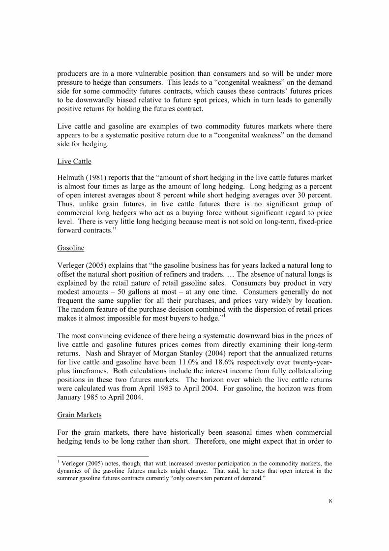
First quarter 2005 returns: 7.1%. Calculations Based on Daily Data from Ryan Duncan, Calyon Financial, 4/1/05. Exhibit 8 shows the yearly simulated returns of pursuing a 240-Day Range Breakout system in the commodity sector. The annual compound returns over the period, 1995 to

18

2004, were 11.3%. In this system, one enters a long position in a commodity if its price is greater than the highest price over the previous 240 days. Correspondingly, one enters a short position in a commodity if its price is less than the lowest price of the previous 240 days.

Exhibit 8

Annual Returns Due to a Commodity-Only Technical Trading Strategy: The Range Breakout System

Returns of CALYON FINANCIAL Trend-Following Strategy: 240-Day Range Breakout System (1995 to 2004)

-50%-40%-30%-20%-10%

0%10%20%30%40%50%

1995 1996 1997 1998 1999 2000 2001 2002 2003 2004

First quarter 2005 returns: 13.2%. Calculations Based on Daily Data from Ryan Duncan, Calyon Financial, 4/1/05. Burghardt et al. (2004) note that “commodity markets tend to be less liquid than financial markets. Many managers, to get around the constraint that illiquid commodities markets would place on their trading capacity, continue to expand by decreasing the weight that commodities play in their portfolio.” In summing up this section we would say that despite the promising results shown in the Calyon study, CTA’s have tended to trade financial rather than natural-resource commodity markets because of the greater liquidity and capacity of the financial markets. The rest of this article will now focus on investing in the commodity futures markets based on identifiable fundamental factors. CRUCIAL ELEMENTS OF AN INVESTMENT PROCESS In this section, we will discuss the crucial elements of an investment process that takes advantage of the fundamental sources of return in the commodity futures markets. We will briefly discuss trade sizing, entry and exit rules, trade construction, portfolio

19

construction, and risk management. We will finish up this article with an important caveat on solely relying on quantitative methods in futures trading. Trade Sizing The discovery of structural sources of return in the commodity futures market is only the first step in designing an investment program. For example, how should one determine how large each individual trading strategy should be? This section will discuss sizing trades based on their risk characteristics. Sizing as a Function of Risk Risk is “the currency of trading,” notes Grant (2004). “Each trading account has … a finite amount of this currency, and it is vital to manage portfolio affairs in such a way that respects this resource constraint.” Volatility An initial way to respect this resource constraint is to size trades according to their recent volatility. One wants to ensure that under normal conditions, a commodity position has not been sized too large that a trader cannot sustain the random fluctuations in profits and losses that would be expected to occur, even without an adverse event occurring. Sizing a trade based on its volatility is especially important the longer the frequency of predictability is. For example, if a trade’s predictability is at quarterly intervals, the trade has to be sized to withstand the daily fluctuations in profits and losses. Worst-Case Loss Using long-term data, one should also examine the worst performance of a commodity trade under similar circumstances in the past. In practice, such a measure will sometimes be larger than a measure based on recent volatility. In that case, the trade size should be further scaled down to reflect the worst-case loss. Examining the worst-case outcomes can also serve another purpose. If the loss on a particular commodity futures trade exceeds the historical worst case, this can be an indication of a new regime that is not reflected in the data. This would trigger an exit from a systematic trade since one no longer has a handle on the worst-case scenario. This point will be further discussed below in the Entry and Exit Rules section of this article. Optimal Sizing The equity markets have shaped the professional experiences of most financial market participants. This can present a problem for a new participant to the commodity markets. Unlike equities, most commodity price distributions are positively skewed. This is because of the asymmetric nature of storage. If there is too much of a commodity, some

20

of it can be stored and the price can decline to encourage the placement of the commodity. The existence of storage can dampen the price decline because this is an additional lever with which to balance supply and demand. On the other hand, if there is too little of a commodity, then that means there are inadequate inventories and therefore the only lever available to balance supply and demand is price, which must correspondingly increase. The inability of “the market as a whole to carry negative inventories,” as Deaton and Laroque (1992) put it, causes commodity markets to be prone to violent upward price spikes. Exhibits 9 and 10 provide examples from the copper and corn markets, which show how explosive commodity prices can be during times of low inventories relative to consumption.

Exhibit 9

Copper Prices versus Normalized Inventories

0.60

0.80

1.00

1.20

1.40

1.60

1.80

2 4 6 8 10 12 14 16 18

Average Inventory/Weeks Consumption

LME

Pric

e C

onst

ant U

S$/lb

Data Source: RBC Dominion Securities.

21

Exhibit 10

Corn Prices versus Normalized Inventories

CORN PRICE ANALYSISMarch USDA Supply/Demand

91

92

93

94

95

96

97

98

9900 01

02

03

04

05

180190200210220230240250260270280290300310320330340350360370380390400410420430440450460

0.03 0.04 0.05 0.06 0.07 0.08 0.09 0.10 0.11 0.12 0.13 0.14 0.15 0.16 0.17 0.18 0.19 0.20 0.21 0.22 0.23 0.24 0.25 0.26 0.27 0.28 0.29

Estimated Carryout/Use Ratio

Pric

e in

Cen

ts p

er B

ushe

l

Source: Everett (2005).

22

Hooker of State Street Global Advisors (2004) confirms the positive skewness of a number of commodity return distributions. Exhibit 11 provides a summary of the skewness of a number of commodities as compared to U.S. equities and bonds.

Exhibit 11

Distribution Moments: Skewness

-0.8-0.6-0.4-0.20.00.20.40.60.81.01.21.4

Crude

Heatin

g Oil

Coppe

r

Coffee Corn

Soybe

ans

Lean

Hog

sGSCI

S&P 500

10-ye

ar Trea

surie

s

Futures Contract

Skew

ness

Source: Excerpted from Hooker (2004), Slide 11. Author’s notes: * “Significant right skew for many commodities, in contrast to the left skew of equities and bonds.” * “Based on monthly futures roll returns, April 1994 to March 2003. Sources: Bloomberg, Goldman Sachs Commodity Index, State Street Global Advisors.” Walton (1991) notes that “the asymmetrical behavior of commodity stocks … means that most price surprises are on the upside. Thus, it makes sense for investors generally to be long of commodities.” When constructing total-return commodity portfolios, one should take into consideration the asymmetric nature of commodity returns as follows. The risk capital allocated to individual long commodity positions needs to be much larger than the capital allocated to individual short commodity positions.

23

Entry and Exit Rules Fung and Hsieh (2003) note that an important source of alpha for systematic futures programs is superior entry/exit strategies. Seasonal Strength and Weakness In order to profit from commercial hedging pressure, Cootner (1967) provides historical examples of profitable entry and exit strategies in the grain futures markets. The author summarizes the results of studies that both he and others carried out, which use data that goes as far back as 1921 and as recently as through 1966. Cootner’s (historically) profitable strategies are keyed off the following factors: (1) peaks and troughs in visible grain supplies, (2) peaks and troughs in hedging positions from data provided by the Commodity Exchange Authority, a predecessor organization to the CFTC, and (3) fixed calendar dates that line up on average with factors (1) and/or (2). Similarly, Girma and Paulson (1998) write that “the gasoline crack spread seasonality seems to parallel the seasonality of the gasoline inventory levels.” And also, the heating oil crack spread reaches peaks and troughs that parallel the heating oil inventory cycle. Using reasoning from Cootner (1967), the turning points for price-pressure effects are on average around peak (trough) inventory levels because that is when hedging by commercials would be at their highest (lowest). Commercials do not generally take advantage of these well-known effects because “for hedgers to profit from the [futures price] bias requires that they be long when they already hold maximum inventories and short when they hold minimum inventories.” Positive Curve Dynamics Another entry and exit signal is based on whether a futures curve for a commodity is in backwardation or not, as covered in the Scarcity section of this article. Structural Break As discussed in the Worst-Case Loss section of the article, if a loss on a particular commodity futures trade exceeds the historical worst case, this can be an indication of a break from past structural phenomena that had been detectable in historical data. In that case, a trader would exit a trade since one no longer has a handle on the magnitude of additional losses. The following is an example of a structural break from the fall of 2003. Up until that point, soybean futures prices typically declined in the face of the U.S. crop harvest. Further, the magnitude of the decline had been largely related to summer weather conditions. From 1980 through 2002, the September-to-October decline in soybean prices could be related to the following three variables: (1) the change in soybean prices during the summer, which historically had been highly correlated with the change in

24

Good-to-Excellent ratings for soybeans, as provided by the U.S. Department of Agriculture; (2) a government loan figure, which served as a proxy for soybean inventories; and (3) a price ratio, which was highly correlated with farmers’ decisions in choosing between planting corn or soybeans. This model had explained 81% of the variation in autumn soybean prices over the twenty-three period, 1980 to 2002. In the fall of 2003, this model predicted a drop in soybeans of about -50c. Instead, soybeans rallied over +60c from early September through early October. From 1980 through 2003, the most that soybeans had rallied in the face of a new US crop harvest was +36c. So once soybeans had rallied to this level, one had an indication that new factors were in place that had not been the case in the past. By exiting the trade at +36c, one limited the ultimate losses from being short soybeans in the face of an explosive rally. According to Cronin (2003), massive Chinese import demand combined with unusually damaged U.S. crops caused soybean prices to rally so as to encourage farmers in the Southern Hemisphere to increase the amount of soybean planting still possible at that time. As of early October 2003, Brazil had only planted 4% of its soybean acres. And as touched upon earlier in the Weather Fear Premia section of the article, Latin American countries now produce a majority of the world’s soybean crops. The new demand (from China) and supply (from Latin America) appeared to cause a structural break in historical soybean price dynamics. The conclusion from this discussion is that a trading program will not experience the full brunt of a structural break if one exits a trading strategy after experiencing losses that are greater than have been the case in the past. Trade Construction As discussed in Till and Eagleeye (2004), one can have a correct commodity view, but how one constructs the trade to express this view can make a large difference in profitability. In the commodity futures markets, one can choose to implement trades through outright futures positions, spreads, and/or options. One can make this decision by examining which implementation has provided the best historical return-to-risk profile. Futures spreads can sometimes be more analytically tractable than outright futures contracts. There is usually some economic boundary constraint that links related commodities, which typically (but not always) limits the risk in position-taking. Also, one hedges out a lot of first-order, exogenous risk by trading spreads. For example, with a heating-oil-vs.-crude-oil futures spread, each leg of the trade is equally affected by unpredictable OPEC shocks. Instead, what typically affects the spread is second-order risk factors like timing differences in inventory changes in the two commodities.

25

Portfolio Construction Diversification Uniquely among asset classes, commodities can offer uncorrelated investment opportunities across individual commodity markets. Moreover, energy-sector commodities are frequently negatively correlated to non-energy-sector commodities. This greatly aids in setting up dampened risk portfolios. The reason for this negative correlation is due to the fact that an energy spike can dampen economic growth, which in turn, dampens demand for other less economically essential commodities, as noted in Till (2001). Further, hedge fund manager Paul Touradji argues, “One of the best things about being a commodity manager is the natural internal diversification.” “While even unrelated equities have a beta to the overall market, many commodities, such as sugar and aluminum, traditionally have no correlation at all,” according to Teague (2004) in his interview with Touradji. Exhibit 12 provides an example from the summer of 2000, which illustrates the portfolio effect on volatility of incrementally adding unrelated commodity strategies.

Exhibit 12

Portfolio Effect of Combining Unrelated Commodity Strategies

Portfolio Volatility vs. Number of Strategies

6.0

7.0

8.0

9.0

10.0

11.0

12.0

13.0

14.0

1 2 3 4 5 6 7

Number of Strategies

Port

folio

Vol

atili

ty

Source: Based on Till (Fall 2000), Exhibit 5.

26

Avoidance of Inadvertent Concentration Risk In order to meet the goal of creating a diversified portfolio, a commodities portfolio manager needs to exercise due care in ensuring that each additional trade is in fact a risk diversifier rather than a risk amplifier. If two trades are in fact related, then one should consider them as part of the same strategy bucket and require them to share risk capital. If each trade is instead allocated full risk capital, then one may be inadvertently doubling up on risk. Natural Gas and Corn Recent correlations will not necessarily be a sufficient guide as to whether two seemingly unrelated trades are in fact separate trades. For example, one might expect the price of natural gas to be unrelated to the price of corn. But in July of 1999, these two markets became 85% correlated with each other. This is because both of these markets are highly sensitive to the outcome of July weather in the U.S. Midwest. For natural gas, a heat wave can cause prices to rally in order to ration demand so that storage injections for peak winter demand will continue on schedule. For corn, a heat wave can be damaging to corn yields during corn’s key pollination time, which in turn would cause corn prices to rally. In July 1999, blistering hot weather did occur, which caused corn and natural gas futures prices to simultaneously rally, which in turn caused them to appear like the same trade. In summary, if a commodity manager included corn and natural gas futures trades in their portfolio during July, then the portfolio would contain concentrated risk to the outcome of U.S. Midwest weather.

27

Platinum and Copper Chinese demand for commodities has become a relatively recent dominant factor in the commodity markets. Exhibit 13 shows the importance of Chinese demand for a number of metals markets.

Exhibit 13

Chinese Metals Demand

Percentage Share of Percentage of Growth Contribution World Demand (1997-2002)

Platinum 25% 90% Copper 17% 70% Zinc 18% 59% Aluminum 18% 57% Nickel 8% 34% Silver 4% 11% Data Source: Excerpted from Smith (2004). Note particularly that the Chinese share of recent growth in platinum demand is 90% while the share of growth for copper demand is 70%.

28

Exhibit 14 shows the time-varying correlation of changes in platinum and copper prices. During the first six months of 2004, the monthly changes in these two markets were +93% correlated while during the next seven months, this correlation was only 17%.

Exhibit 14

Change in Platinum Prices vs. Change in Copper Prices First Six Months of 2004

Front-month Platinum Futures Prices vs. Copper Futures Prices, Monthly Changes, 12/31/03 to 6/30/04

-150

-100

-50

0

50

100

-20 -15 -10 -5 0 5 10 15 20 25

Changes in Copper Prices (Cents per Pound)

Cha

nges

in P

latin

um P

rices

(Dol

lars

pe

r Oun

ce)

Actual Platinum vs. Copper Price Changes Fitted Platinum vs. Copper Price Changes

Change in Platinum Prices vs. Change in Copper Prices Succeeding Seven Months

Front-month Platinum Futures Prices vs. Copper Futures Prices, Monthly Changes, 6/30/04 to 1/31/05

-40

-30

-20

-10

0

10

20

30

40

50

60

-8 -6 -4 -2 0 2 4 6 8 10 12 14

Changes in Copper Prices (Cents per Pound)

Cha

nges

in P

latin

um P

rices

(Dol

lars

pe

r Oun

ce)

Actual Platinum vs. Copper Price Changes Fitted Platinum vs. Copper Price Changes

Data Source: Bloomberg.

29

In early 2005, if a commodity manager only examined the recent correlations of platinum and copper futures prices, then that manager would have missed the two markets’ strong previous relationship, not to mention their common fundamental driver. These two trades need to share the same risk capital because in the event of a Chinese demand shock, there could be similar price responses by both metals contracts, as occurred during the last two weeks of April 2004. At that time, following reports of a more stringent official policy towards industrial loans in China, both copper and platinum prices declined precipitously, as shown in Exhibit 15.

Exhibit 15

Platinum and Copper Prices During the Last Half of April 2004

Daily Platinum and Copper Futures Prices (4/15/04 to 4/30/04)

750

770

790

810

830

850

870

890

910

930

950

4/15/2

004

4/16/2

004

4/19/2

004

4/20/2

004

4/21/2

004

4/22/2

004

4/23/2

004

4/26/2

004

4/27/2

004

4/28/2

004

4/29/2

004

4/30/2

004

Date

Plat

inum

Pric

es ($

per

oun

ce)

105

110

115

120

125

130

135

140

Cop

per P

rices

(c p

er p

ound

)

July 2004 Platinum Prices May 2004 Copper Prices

Data Source: Bloomberg.

30

Energy Spreads When managing an absolute-return commodity program, one may want to limit the amount of “beta risk” that a portfolio has to a particular commodity. Exhibit 16 illustrates an example from March 2005. At that time, an energy sub-portfolio consisted of petroleum-complex intramarket and intermarket spreads as well as natural gas futures contracts. The sensitivity of the portfolio’s energy positions to front-month gasoline prices almost doubled from the original period of study, 12/1/04 to 2/22/05, as compared to a later timeframe, 2/22/05 to 3/22/05.

31

Exhibit 16

Changing Sensitivity of a Portfolio to Gasoline Prices

Energy Basket Value vs. Front-Month Gasoline Prices, Daily Changes, 12/1/04 to 2/22/05

(8,000)

(6,000)

(4,000)

(2,000)

-

2,000

4,000

6,000

8,000

(4,000) (3,000) (2,000) (1,000) - 1,000 2,000 3,000

Change in Value of Gasoline Contract in $

Cha

nge

in V

alue

of E

nerg

y B

aske

et in

$

Actual Energy Basket vs. Gasoline Prices Fitted Energy Basket vs. Gasoline Prices

Beta = 1.4 R-squared = 46%

Energy Basket Value vs. Front-Month Gasoline Prices, Daily Changes, 2/22/05 to 3/22/05

(8,000)

(6,000)

(4,000)

(2,000)

-

2,000

4,000

6,000

8,000

10,000

12,000

(3,000) (2,000) (1,000) - 1,000 2,000 3,000 4,000

Change in Value of Gasoline Contract in $

Cha

nge

in V

alue

of E

nerg

y B

aske

t in

$

Actual Energy Basket vs. Gasoline Prices Fitted Energy Basket vs. Gasoline Prices

Beta = 2.4 R-squared = 76%

Data Source: Bloomberg

32

If a manager had intended that their actively managed commodity portfolio should have limited exposure to the outright direction of commodity prices, then this doubling of exposure to the fortunes of front-month gasoline may have been unacceptable. Long-Option-Like Payoff Profile A final consideration in combining trading strategies is to attempt to ensure that the portfolio will have a long-option-like payoff profile. The traditional investors for futures products (which include global macro funds as well as CTA’s) have historically expected a great deal of long optionality from them. Confirming this point, Grant (2004) notes that global macro traders should have an additional objective besides a return threshold. He provides a benchmark objective for the “performance ratio,” which is the ratio of average daily gains divided by average daily losses. Based on Grant’s experience, a performance objective “in the range of 125% is entirely achievable … [although some traders can exceed that], consistently achieving 200%+ in this regard.” The Optimal Sizing section of this article noted the importance of allocating a disproportionate amount of risk capital to individual long commodity positions, which tend to have positively skewed outcomes, relative to the amount of risk taken with individual short commodity positions, which correspondingly tend to have negatively skewed outcomes. This trade construction methodology increases the chances of a portfolio having a long-option-like payoff profile over time.

33

Exhibit 17 shows a commodity futures portfolio return analysis from August of 2004, which shows how the portfolio would have performed from 1981 through 2003.

Exhibit 17

Verification of (Historical) Long-Options-Like Profile

Portfolio Return

-5.0%

0.0%

5.0%

10.0%

15.0%

20.0%

25.0%

1981

1983

1985

1987

1989

1991

1993

1995

1997

1999

2001

2003

Source: Premia Capital Management, LLC Risk Management Value-at-Risk As noted in Till (2002), in the standard Value-at-Risk (VAR) approach, one calculates the portfolio’s volatility based on recent volatilities and correlations of the portfolio’s instruments. If a portfolio of instruments is normally distributed, one can come up with the 95% confidence interval for the portfolio’s change in monthly value by multiplying the portfolio’s recent monthly volatility by two (or 1.96, to be exact.) Now, this approach alone is obviously inadequate for a commodity portfolio, which consists of instruments that have a tendency towards extreme positive skewness. As noted in the Trade Sizing section of this article, the measure is useful since one wants to ensure that under normal conditions, a commodity position (or portfolio) has not been sized so large that one cannot sustain the random fluctuations in profits and losses that might ensue.

34

For a more full representation of risk, one also needs to use VAR in concert with appropriate scenario tests. Scenario Testing In Till (2002), we recommend using long-term data to directly examine the worst performance of a commodity trade under similar circumstances in the past. In practice, such a measure will sometimes be larger than a Value-at-Risk measure based on recent volatility.

Because a commodity investment is frequently intended to be a hedge for a financial portfolio, a commodity manager should also examine the portfolio’s sensitivity to a number of events based on historical data. If the commodity portfolio would do particularly poorly during times when the financial markets performed poorly, then this may be disappointing for a manager’s clients. Event Risk: Sharp Shock to Business Confidence Although a commodity futures portfolio may contain no financial futures contracts, the portfolio could still have systematic risk to the stock market. For example, Bessembinder (1992) found that live cattle and platinum futures had statistically significant betas to the U.S. stock market using data from 1967 to 1989. A manager should therefore consider examining what the portfolio’s performance would have been during the October 1987 stock market crash, the 1990 Gulf War, the Fall 1998 bond debacle, and during the immediate aftermath of September 11, 2001. If the commodity portfolio would have done poorly during these events, then the manager may consider buying macro-portfolio insurance against these events, which is covered below. Event Risk: Extreme Weather Outcomes A key reason for the existence of commodity futures markets is because of the uncertainty surrounding weather. We already noted in the Avoidance of Inadvertent Concentration Risk section how the outcome of U.S. Midwest weather during July is a key influence on the prices of both corn and natural gas futures contracts. Another example is during the month of February. This is a key time for determining the prices of both natural gas and heating oil prices. As one nears the end of the winter in the U.S., utilities are drawing from storage for both commodities to provide for heating demand. If there is extremely cold weather, price is the main variable which balances supply and demand since inventories of natural gas and heating oil are approaching their seasonal lows at this time of year. In this case, their prices can both respond explosively to extremely cold weather. What this means for the commodity manager is that one should consider examining how an energy portfolio would have performed during those rare times of extreme weather during the month of February.

35

Macro Portfolio Hedges If losses would have exceeded a threshold amount during any of a program’s event-risk scenarios, then a manager should consider implementing macro-portfolio hedges, which would do well during the relevant scenario. Rajagopal (2004) notes that a commodity-index investment provides “tail protection for fixed income.” In other words, during those quarters where bonds had negative performance, commodities cumulatively performed well over the period, 1992 to 2004. For a portfolio that has a long commodity bias, one can also state the converse: long fixed-income positions can provide event-risk protection for a commodity portfolio. This is illustrated in Exhibit 18.

36

Example Risk Report Exhibit 18 provides an example strategy-level risk report, which shows the Value-at-Risk and Worst-Case scenarios at both the strategy and portfolio level. (The events used in Exhibit 18’s risk report were defined in the Event Risk: Sharp Shock to Business Confidence section of this article.) Note that a deferred long position in Eurodollar futures reduces the portfolio’s risk to extreme financial events.

Exhibit 18 Strategy-Level Analysis

8/11/2004

Worst-Case Loss Worst-Case LossStrategy Value-At-Risk During Normal Times During Eventful Period

1 Gasoline Front-to-Back Spread 2.59% -5.59% -4.31%

2 Deferred Outright Gasoline 3.81% -2.50% -2.76%

3 Deferred Outright Natural Gas 0.67% -0.15% -0.29%

4 Deferred Eurodollar Futures 2.42% -5.92% -0.96%

5 Hog Spread 3.87% -2.66% -3.23%

6 Deferred Gasoline Spread 1.60% -0.29% -0.53%

7 Cattle Spread 1.62% -0.50% -1.34%

Portfolio 9.24% -8.89% -2.27%

Incremental Contribution to Incremental Contribution to Portfolio Value-at-Risk* Worst-Case Portfolio Event Risk*

Strategy1 Gasoline Front-to-Back Spread 1.62% 0.64%

2 Deferred Outright Gasoline 2.93% -0.72%

3 Deferred Outright Natural Gas 0.52% 0.16%

4 Deferred Eurodollar Futures 0.77% -2.86%

5 Hog Spread 1.18% -0.29%

6 Deferred Gasoline Spread 1.33% 0.29%

7 Cattle Spread 0.25% -0.32%

* A positive contribution means that the strategy adds to riskwhile a negative contribution means the strategy reduces risk.

NotesWhile under "normal" times, the gasoline spread position is less risky than the outright, during particular "eventful" timesthe spread adds to risk while the outright reduces risk.

While under "normal" times, the Eurodollar futures position adds to risk, during particular "eventful" times this interest-rateposition reduces risk.

Source: Premia Capital Management, LLC

37

Caveat on the Crucial Elements of an Investment Process: An Investor’s Risk Tolerance Gehm (2004) lay down a challenge to financial-market writers. This author of the 1995 book, Quantitative Trading and Money Management, said that most financial literature is unrealistic. If financial articles were realistic, they would include both the joys and tears of trading. We will now provide a small window into what Gehm is referring to. In discussing the crucial elements of an investment process, we have left out one vital aspect of trading, and that is a manager’s risk tolerance. Vince (1992) states that monetizing market inefficiencies “requires more than an understanding of money management concepts. It requires discipline to tolerate and endure emotional pain to a level that 19 out of 20 people cannot bear. … Anyone who claims to be intrigued by the ‘intellectual challenge of the markets’ is not a trader. The markets are as intellectually challenging as a fistfight. … Ultimately, trading is an exercise in self-mastery and endurance.” This article has thus far not emphasized the psychological discipline that is required to carry out successful futures trading. But this factor is just as crucial as finding structural sources of return and designing an appropriate risk management methodology around them. Taleb (2001) explains why it is a challenge for a manager to follow a disciplined investment process. He provides an example of a return-generating process that has annual returns in excess of T-bills of 15% with an annualized volatility of 10%. At first glance, one would think it should be trivial to carry out a trading strategy with such superior risk and return characteristics. But Taleb also notes that with such a return-generating process, there would only be a 54% chance of making money on any given day. If the investor felt the pain of loss say 2.5 times more acutely than the joy of a gain, then it could be potentially exhausting to carry out this superior investment strategy. As a further example of the challenge of carrying out a disciplined investment process, this article provided an example of a heating oil calendar spread that had been published in 1989. Of note is that this strategy has continued to work in some form during the past 15 years. But, while this strategy has been demonstrably statistically significant, its maximum loss has been such that this loss could erase the previous year and a half of the strategy’s profits. The result is that if a manager experienced a loss of this magnitude, both the manager (and his or her investors) would need to be quite disciplined to continue carrying out this strategy.

38

CONCLUSION Given how strong the case is for an indexed investment in commodities, one should be quite careful in recommending an actively managed commodity program. That said, skilled active managers can potentially provide returns over an investor’s core indexed commodity exposure. This article discussed persistent sources of return in the commodity futures markets. But we noted that this is not enough for an actively managed commodity program to be successful. A successful futures program also requires extra care in risk management and exceptional discipline in implementation. ENDNOTE The authors wish to express gratitude to Mr. Jerry Pascucci of Citigroup’s Managed Futures department for support of Premia Capital’s investment methodology.

39

BIBLIOGRAPHY Abken, Peter, “An Analysis of Intra-Market Spreads in Heating Oil Futures,” Journal of Futures Markets, September 1989, pp. 77-86. Akey, Rian, “Commodities: A Case for Active Management,” Working Paper, Cole Partners, 2/4/05. Asness, Cliff, Jacques Friedman, Robert Krail, and John Liew, “Style Timing: Value versus Growth,” Journal of Portfolio Management, Spring 2000, pp. 50-60. Bessembinder, Hendrik, “Systematic Risk, Hedging Pressure, and Risk Premiums in Futures Markets,” The Review of Financial Studies,” Vol 5, Number 4 (1992) pp. 637-667. Bodie, Zvi, and Victor Rosansky, “Risk and Return in Commodity Futures,” Financial Analysts Journal (May-June 1980), pp. 27-39. Burghardt, Galen, Ryan Duncan, and Lianyan Liu, “What You Should Expect From Trend Following,” Calyon Financial Research Note, 7/1/04. Center for International Securities and Derivatives Markets (CISDM) 2nd Annual Chicago Research Conference, 5/22/02. Cronin, Walter (professional grain futures trader), private correspondence, 10/4/03. Cochrane, John, “New Facts in Finance,” Economic Perspectives, Federal Reserve Board of Chicago, Third Quarter, 1999. Cootner, Paul, “Speculation and Hedging.” Food Research Institute Studies, Supplement, 7, (1967), pp. 64-105. Cordier, James, “My Best Trade,” Trader Monthly, April/May 2005, p. 44. Deaton, Angus, and Guy Laroque, “On the Behavior of Commodity Prices,” Review of Economic Studies, (1992) 59, pp. 1-23. Duncan, Ryan, Calyon Financial, private correspondence, 4/7/05. Di Tomasso, John and Hilary Till, “Active Commodity-Based Investing,” Journal of Alternative Investments, Summer 2000, pp. 70-80. Erb, Claude and Campbell Harvey, “The Tactical and Strategic Value of Commodity Futures,” Working Paper, Trust Company of the West and Duke University, 2/11/05. Everett, Bevan “FCStone Grain Recap,” 3/18/05, p. 1.

40

Fung, William and David Hsieh, “The Risk in Hedge Fund Strategies: Alternative Alphas and Alternative Betas,” a chapter in The New Generation of Risk Management for Hedge Funds and Private Equity Investments (Edited by Lars Jaeger), Euromoney Books, 2003, pp. 72-87. Gehm, Fred, “Risk Management in Hedge Fund of Funds Panel,” Presentation at Chicago Professional Risk Managers’ International Association (PRMIA) meeting, 12/16/04. Gillman, Pat (Chicago commodities law attorney), private correspondence, 4/4/05. Girma, Paul and Albert Paulson, “Seasonality in Petroleum Futures Spreads,” Journal of Futures Markets, August 1998, pp. 581-598. Grant, Kenneth, Trading Risk, Wiley Trading, 2004. Greer, Robert, “Commodities – Commodity Indices for Real Return and Diversification,” a chapter in The Handbook of Inflation Hedging Investments (Edited by Robert Greer), McGraw Hill, forthcoming 2005. Helmuth, John, “A Report on the Systematic Downward Bias in Live Cattle Futures Prices,” Journal of Futures Markets, March 1981, pp. 347-358. Hicks, J.R., Value and Capital, Oxford University Press, 1939. Hooker, Mark, “Portfolio Risk Measures,” State Street Global Advisors, Presentation at IQPC Conference on Portfolio Diversification with Commodity Assets, London, 5/26/04. Humphreys, H. Brett, and David Shimko, “Beating the JPMCI Energy Index,” Working Paper, JP Morgan, August 1995. Keynes, John, A Treatise on Money, Macmillan and Company Limited, 1934. Lammey, Alan, “Investors Clamor for Stake in Bull Run in Stocks, Commodities,” Natural Gas Week, 4/4/05, p. 19. Maddala, G.S., and Jisoo Yoo, “Risk Premia and Price Volatility in Futures Markets,” Center for the Study of Futures Markets, Columbia Business School, Working Paper Series CSFM #205 (July 1990). Nash, Daniel and Boris Shrayer, “Morgan Stanley Presentation,” IQPC Conference on Portfolio Diversification with Commodity Assets, London, 5/27/04. Rajagopal, Mohan, “Examining the Financial Benefits of Commodities and Practical Issues of Implementation,” Deutsche Bank, Presentation at Marcus Evans Conference on Investing in Commodities, London, 11/8/04.

41

Rosenberg, Barr, Kenneth Reid, and Ronald Lanstein, “Persuasive Evidence of Market Inefficiency,” Journal of Portfolio Management, Spring 1985, pp. 9-16. Rowland, Heather, “How Much Oil Inventory is Enough?,” Energy Intelligence Group, 1997. Siegel, Laurence, Benchmarks and Investment Management, Association for Investment Management and Research, Charlottesville, Va., 2003. Smith, Andy, “Precious Thoughts,” Mitsui Global Precious Metals, 4/29/04. Taleb, Nassim, Fooled By Randomness, Texere, 2001. Teague, Solomon, “The Commodities ‘Gladiator’,” Risk Magazine, p. 88. Teweles, Richard and Frank Jones, The Futures Game, McGraw-Hill Book Company, 1987. Till, Hilary, “Systematic Returns in Commodity Futures,” Commodities Now, September 2000, pp. 75-79. Till, Hilary, “Trading Scarcity,” Futures magazine, October 2000, pp. 48-50. Till, Hilary, “Passive Strategies in the Commodity Futures Markets,” Derivatives Quarterly, Fall 2000, pp. 49-54. Till, Hilary, “Laughing in the Face of Diversity,” Risk & Reward, February 2001, pp. 18-21. Till, Hilary, “Risk Management Lessons in Leveraged Commodity Futures Trading,” Commodities Now, September 2002, pp. 84-87. Till, Hilary, “On the Role of Hedge Funds in Institutional Portfolios,” Journal of Alternative Investments, Spring 2004, pp. 77-89. Till, Hilary and Joseph Eagleeye, “How to Design a Commodity Futures Trading Program,” a chapter in Commodity Trading Advisors: Risk, Performance Analysis, and Selection (Edited by Greg Gregoriou, Vassilios Karavas, Francois-Serge L’Habitant, and Fabrice Rouah), Wiley Finance, 2004, pp. 277-293. Verleger, Philip, “Inflating the Commodity Bubble: Impact of Pension Fund Investment on Oil Prices,” The Petroleum Economics Monthly, January 2005. Vince, Ralph, The Mathematics of Money Management, Wiley Finance, 1992. Walton, David, “Backwardation in Commodity Markets”, Working Paper, Goldman Sachs, 5/28/91.

42

Working, Holbrook, “Theory of the Inverse Carrying Charge in Futures Markets,” Journal of Farm Economics, February, 1948, pp. 1-28.