COMMISSION STAFF WORKING DOCUMENT - Europa

EN EN

COMMISSION OF THE EUROPEAN COMMUNITIES

Brussels, 16.12.2008 SEC(2008) 3054

COMMISSION STAFF WORKING DOCUMENT

Accompanying document to the

COMMUNICATION FROM THE COMMISSION TO THE EUROPEAN PARLIAMENT, THE COUNCIL AND THE EUROPEAN COURT OF AUDITORS

Towards a common understanding of the concept of tolerable risk of error

{COM(2008) 866 final}

2

COMMISSION STAFF WORKING DOCUMENT

Towards a common understanding of the concept of tolerable risk of error

1. SCOPE ............................................................................................................................................................... 3

2. APPROACH AND ASSUMPTIONS............................................................................................................... 3

2.1 THE LINK BETWEEN RESIDUAL RISK AND COST OF CONTROLS............................................... 3

2.2 MODELLING THE RELATIONSHIP BETWEEN THE COST AND THE RATE OF UNDETECTED ERRORS ................................................................................................................................... 4

2.2.1 Linear model......................................................................................................................................... 4 2.2.2 Extending the linear model................................................................................................................... 5 2.2.3 Testing the model.................................................................................................................................. 7

2.3 GENERAL ASSUMPTIONS AND CALCULATION METHODS............................................................ 8

2.3.1 General assumptions: ........................................................................................................................... 8 2.3.2 Calculations and methods..................................................................................................................... 9

2.4 ILLUSTRATIVE CASES............................................................................................................................. 11

2.4.1 European Regional Development Fund (ERDF)................................................................................ 11 2.4.2 European Agricultural Fund for Rural Development (EAFRD)......................................................... 15

3. THE COST OF CONTROLS EXERCISE ................................................................................................... 17

3.1 METHODOLOGY........................................................................................................................................ 17

3.2 RESULTS FOR THE COMMISSION SERVICES................................................................................... 18

3.2.1 European Agricultural Guidance and Guarantee Fund (EAGGF) .................................................... 18 3.2.2 European Regional Development Fund (ERDF)................................................................................ 19 3.2.3 DG Employment and Social Affairs.................................................................................................... 20 3.2.4 DG EuropeAid .................................................................................................................................... 21 3.2.5 DG Environment................................................................................................................................. 21 3.2.6 DG Research ...................................................................................................................................... 22 3.2.7 DG Information Society...................................................................................................................... 22 3.2.8 Other Services .................................................................................................................................... 23

GLOSSARY: ....................................................................................................................................................... 24

3

1. SCOPE The aim of this document is to present the technical elements supporting the conclusions and the analysis set out in the accompanying Communication COM(2008) 866. The document presents the approaches taken in respect of selected policies of the Commission for the illustrative examples in the main communication, together with a first estimation of the costs of controls for selected policies (results of Action 10 of the Action Plan towards an Integrated Internal Control Framework) in both direct centralised mode and shared management mode. 2. APPROACH AND ASSUMPTIONS

2.1. The link between residual risk and cost of controls

Controls cost money and a cost-effective balance has to be sought between the number of controls and the amounts of error detected and recovered. The more controls that are carried out, the lower the rate of undetected error will be. This intuitive relationship between the level of errors undetected by Commission and Member States' controls and cost of controls is shown in the following chart:

Graph 1

The following components of the curve can be distinguished, each with its own elasticity:

• Zone 1: In the absence of any control: a theoretical level of "errors" would remain undetected, the nature and value of which depend on the complexity of the regulatory framework, the propensity to error, the inherent risk etc.

Zone 1 Zone 2

Zone 3

Zone 4

Zone 5

Rate of errors undetected by Commission and Member States

Cost of controls

DAS rate

Current (improved) error rate

Increase of the rate of on-the-spot controlsCurrent costs

4

• Zone 2: (Quasi) Fixed costs: or the cost of setting up the control system before controls are carried out (in terms of strategy chosen, risk analysis, definition of tools and procedures).

• Zone 3: Reverse economies of scale: gradual reduction of the error rate while increasing the costs of control (due to great level of elasticity at this point of the curve); at a critical threshold (which we call the "tolerable risk point"), the marginal benefit of an additional control equals the marginal cost of an additional control. Beyond this point the marginal cost of a control exceeds the marginal benefit to be expected (in terms of a reduction in the error rate or the amount of error likely to be detected and recovered).

• Zone 4: “One-off” errors: once the most important and/or systemic errors have been eliminated, only “one-off” errors will exist. Because of their nature, such errors require significant resources in order to be detected.

• Zone 5: Tangent to the 0% error rate: the last remaining errors will require more resources to detect them due to the low level of elasticity at this point of the curve (ultimately all activities will need to be checked completely to identify these errors).

While this is a sound theoretical presentation of the issues, it would be very difficult to draw the “real” curve reflecting the reality of each policy area. In order to identify the coordinates of the points of the curve extensive data would be needed to model the impact of different levels of control - something that is not feasible in practice. It is for example not possible to model the impact of the removal of all controls to define a rate of undetected errors in zone 1.

The process of estimating accurately the cost of control and obtaining reliable data to estimate potential error rates would also imply an extensive data collection exercise, in particular at Member State and implementing body level since detailed statistics are currently not available (for example the number and value of ongoing projects). However, on the basis of available 2006 data complemented by data collected by the Commission on the costs of control, this document sets out some illustrative examples of tolerable risk using a variety of assumptions which are set out in section 2.3 below.

2.2. Modelling the relationship between the cost and the rate of undetected errors 2.2.1. Linear model

The basis for the illustrative examples of tolerable risk presented in this document is a simple linear model in which the rate of undetected error decreases as more controls are carried out. The model presents how one variable (error rate) is related to other variables (principally the cost of control and the numbers of projects/beneficiaries to be controlled). The model presents the situation where one Y variable (the error rate) is related by a straight line to just one X variable (cost of controls). A trend line is then drawn between two known points using a Cartesian equation of the type Y = cX + b where 'c' is the (negative) slope and 'b' the intercept resulting in a distribution (or population) of Y values, appropriately called the probability distribution of Y1 given X1, and similarly a distribution of Y2 at X2, and so forth. The population parameters b and c specify the straight line, known as the true population regression line and are estimated from the available information on control costs and error

5

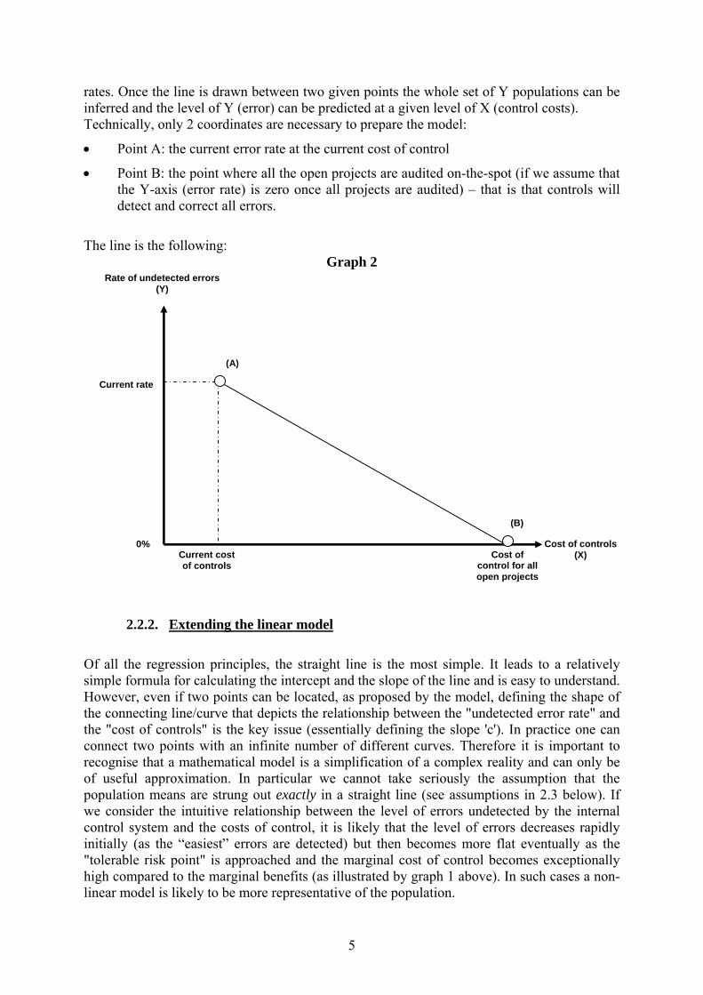
rates. Once the line is drawn between two given points the whole set of Y populations can be inferred and the level of Y (error) can be predicted at a given level of X (control costs). Technically, only 2 coordinates are necessary to prepare the model:

• Point A: the current error rate at the current cost of control

• Point B: the point where all the open projects are audited on-the-spot (if we assume that the Y-axis (error rate) is zero once all projects are audited) – that is that controls will detect and correct all errors.

The line is the following:

Graph 2

2.2.2. Extending the linear model

Of all the regression principles, the straight line is the most simple. It leads to a relatively simple formula for calculating the intercept and the slope of the line and is easy to understand. However, even if two points can be located, as proposed by the model, defining the shape of the connecting line/curve that depicts the relationship between the "undetected error rate" and the "cost of controls" is the key issue (essentially defining the slope 'c'). In practice one can connect two points with an infinite number of different curves. Therefore it is important to recognise that a mathematical model is a simplification of a complex reality and can only be of useful approximation. In particular we cannot take seriously the assumption that the population means are strung out exactly in a straight line (see assumptions in 2.3 below). If we consider the intuitive relationship between the level of errors undetected by the internal control system and the costs of control, it is likely that the level of errors decreases rapidly initially (as the “easiest” errors are detected) but then becomes more flat eventually as the "tolerable risk point" is approached and the marginal cost of control becomes exceptionally high compared to the marginal benefits (as illustrated by graph 1 above). In such cases a non-linear model is likely to be more representative of the population.

Rate of undetected errors (Y)

Cost of controls (X)

Current rate

Current cost of controls

0% Cost of

control for all open projects

(A)

(B)

6

Since the fundamental problem of the model comes down to defining slope 'c', the linear model was extended by adding a trend line to the straight line to reflect a line sloping downward, representing decreased error rates over increasing costs of control. Since the population used for this exercise does not meet the assumption of homogeneity (because different projects present different types and levels of risk), a "logarithmic trend line" is appropriate, as a logarithmic scale shows variable growth changes percentage-wise (whereas a linear trend line is used for constant rates). Therefore a logarithmic trend line is a best-fit curved line that is most appropriate when the rate of change in the data increases or decreases quickly and then levels out.

The logarithmic equation for calculating trend lines calculates the "best line" through points by using an equation of the type y = c ln x + b where c and b are constants, and ln is the natural logarithm1 function. A graphic representation of this trend line is shown in graph 3:

Graph 3

Once the curve is drawn, the level of Y (error) can be predicted at a given level of X (control costs). This means the coordinates of an optimal level of control or the cost of control for a given error rate (for example the cost of achieving the 2% materiality criterion used by the European Court of Auditors) can be estimated.

1 In mathematics, the logarithm of a number to a given base is the power or exponent to which the base must be raised in order to produce the number. For example, the logarithm of 1000 to the base 10 is 3, because 10 raised to the power of 3 is 1000. In the logarithmic trend line, ln(x) stands for the natural logarithm of . To compute a logarithmic trend line one must plot x against “log y” (for example x1,log y1) and (x2, log y2), then draw a straight line between these points on a graph and calculate the equation of the gradient using Y = cX + b


Cost of control (X)

Current rate

Current cost of control

0% Cost of

control for all open projects

Cost of control at Tolerable Risk Point

Rate at Tolerable Risk Point

(A)

(B)

Tolerable Risk Point

7

2.2.3. Testing the model

It is essential to acknowledge that the shape of the curve can have a material difference in setting the optimal level of controls. Therefore the model was tested using more sophisticated mathematical approaches. The following modifications of the model were introduced:

• introduction of "control scope" (% of projects) (A)

• introduction of a more realistic parabolic equation for the cost of control function, taking account of fixed and variable costs (B)

• introduction of the concept of "opportunity cost" (C) and a "combined cost curve" (D), combining the cost of controls and the opportunity cost

• introduction of a "benefit curve" (consisting of recovery order), current benefit being equal to zero (E)

• introduction of "proceeds curve" (benefit– control costs) (F)

• making use of "optimisation" problem solving (maximising proceeds/minimising costs)

Graphically this would lead to five curves:

Graph 4

Control scope (% of projects)

Op

port

uni

ty/c

ont

rol C

ost

Control costs (modified)

Opportunity cost

Combined cost

Benefit (recovered errors)

proceeds (benefit - controlcos t)

(B)

(C)(D)

(E)(F)

(A)

When tested within the limits of the available data, the tests were found to produce comparable results (see below). The simplified model is therefore believed to be reasonably reliable and to provide a sound basis for a first indication of where the tolerable risk point may lie.

8

2.3. General assumptions and calculation methods

The use of regression relies heavily on the underlying assumptions being satisfied. In this model, the following hypotheses were made:

2.3.1. General assumptions:

The following assumptions could potentially cause the tolerable risk point to be overestimated:

• Absence of "lurking" variables: in observational studies, it is essential to eliminate

bias. For this reason some existing models make use of confounding variables called "lurking" variables to take into account more than one independent variable and reduce bias. This is not the case in the model used as many benefits are difficult to quantify (such as the additional reduction of errors through the deterrent effect of controls over and above any specific error detected, the benefits beyond spending, the reputational risk of the Commission due to fraud, etc). Analysis at this stage was therefore limited to cost and benefits of controls in purely quantifiable financial terms.

• All projects need to be controlled to secure 0% error: even if theoretically the control chain should be designed to provide "assurance" to final beneficiary level, the only way to really ensure 100% regularity and legality of underlying transactions is through on-the-spot controls of all projects at a moment when all costs can be fully verified.

• Extrapolation of errors: the model excludes extrapolation of errors (application of corrections of systemic errors to non-audited projects) and therefore requires 100% audit coverage since all projects need to be controlled to eliminate all errors.

• The cost of controls axis is project-based2, meaning that each control is assumed to cost the same amount and there are no economies of scale from simultaneous auditing of several projects for the same beneficiary.

• Homogeneity of the population: when a straight line is used, the population of projects is assumed to be homogeneous in size and in terms of risk of error. Technically this means all the Y distributions have the same spread. This is not likely to be the case in reality since certain types of projects may for example have higher error rates than others. An optimal approach would allow stratification of the projects according to risk, taking account of policy area, size and nature of the activity, management mode or beneficiary where controls would be directed towards higher risk areas thereby reducing risk of undetected error at a lower cost.

Two further assumptions in the model could potentially cause the tolerable risk point to be underestimated: • improving existing controls to reduce the error rate, for example through better

guidance and training, is assumed to have zero cost.

2 While 'project' is a word which has many different meanings within the Commission, it is used in this exercise in the context of the Structural Funds and CAP policy areas.

9

• Audit risk: the model excludes the audit risk (the risk of a control not detecting an existing error) as it assumes that an error rate of 0% would be obtained if all projects were controlled. By excluding the "false negatives" and assuming that controls carried out identify and correct all errors in a project, we distance ourselves from the standard control frameworks that rely on the concept of "reasonable assurance" used to acknowledge that even the best control system cannot avoid all errors and an increased number of controls could never produce a zero level error.

Furthermore three general assumptions are made:

• The control strategy is annual: eliminating all errors on an annual basis would require each project to be audited at the end of each year (to match with the annual opinion of the Court of Auditors required by the Treaty), although this is not likely to be feasible in reality.

• The economic trade-off between costs and benefits is only valid as a hypothesis insofar as the amount of error detected and recovered resulting from an additional control is consequently re-allocated for additional controls.

• The examples provided are based on a single year and it is assumed that this year is representative.

2.3.2. Calculations and methods:

2.3.2.1. Current rate (point A):

To fully understand the methodology presented in this working document, it is essential to distinguish the errors detected by the ex ante internal control chain of the Commission and its implementation partners (therefore proving the efficiency of its controls put in place) from those discovered by the European Court of Auditors, whose findings are outside this control chain. Since many of the projects audited in the Court's annual sample will not have been subject to the full set of controls required by legislation over the lifespan of programmes, the multiannual corrective mechanisms in place (e.g. for cohesion policy) impact the longer-term error rate. The (annually-based) tolerable risk point in this illustrative example is therefore totally distinct from the error level at the closure of each individual (multi-annual) programme.

The methodology used only focuses on the errors that the internal control chain had not prevented or detected at the time of the Court's audit. The current rate of error in the calculations in this document is therefore based on the findings of the Court of Auditors in their annual reports where possible. This estimation constitutes the first point for the construction of the whole model.

It is important to bear in mind the underlying EU control concept where ex-ante controls are of utmost importance as a preventive tool and ex-post controls fulfil a monitoring function as well as acting as corrective controls. In order not to focus disproportionately on the corrective ex-post controls only, the estimated benefits of improving the existing ex ante controls at limited or no significant additional cost were also brought into the equation (using the DAS 2006 "substantive findings" i.e. findings with financial impact according to the Court methodology).

10

2.3.2.2.Cost of control for all open projects (point B):

While it could be worthwhile to invest additional resources in desk-based and on-the-spot ex-ante controls, these controls cannot detect and correct all types of errors. It is also necessary to go on-the-spot to fully control an activity ex-post. Controls on the spot by the audit bodies are therefore necessary to check in detail the legality and regularity of underlying transactions.

Point B (situated on the X-axis) is calculated by multiplying the number of open projects not controlled (the total population to be controlled) by the average cost of an on-the-spot control for each policy and adding the product to the current control cost. The fact that the cost of controlling every project on-the-spot is estimated does not mean that every cost claim has been audited but rather that each open project is assumed to be controlled once annually. Other methods were considered for this modelling but the available data were insufficient to support these.

2.3.2.3.The tolerable risk point:

The optimal trade-off between costs and benefits is based on the concept of marginal benefit, being the decrease in error (defined as the amount of error likely to be detected and corrected by a control) resulting from a unit increase in terms of control cost. In this logic, it is worth carrying out additional controls as long as an additional Euro spent on controls leads to a reduction of the error of more then one Euro3. The tolerable risk point (represented by a star on graph 5) corresponds to the point where the marginal benefit of an extra control becomes equal to its marginal cost. Beyond this point an extra euro spent on controls would exceed the benefits obtained from this additional euro. This means that from a purely economic viewpoint the tolerable risk of error would not be set lower than this "tolerable risk point". Graphically this point is represented by the slope of the tangent of the curve that depicts the cost-benefit relationship. The point where the tangent and the curve touch is the point at which the angle of the curve is 45°/135°, which means that an additional euro spent on control at this exact point would result in an error of one euro being detected and corrected. Mathematically, at this shared point, the first derivative of the curve is equal to the slope of the line (45° tangent gradient)4.

3 In technical terms a positive net benefit corresponds to the ratio "benefit derived from marginal increase of cost of controls/ marginal increase in terms of cost of control" being greater than one. 4 Mathematically the slope, or derivative, of f(x) at point x is the limit, as h approaches zero, of [f(x+h)-f(x)]/h. Note that the tangent for an 45° radian angle (arithmetically equal to '1') is the inverse tangent of an 135° radian angle (arithmetically equal to '-1').

11

For a negative slope we get the following graphical representation:

Graph 5

In theory it could be that for certain areas there would be no tolerable risk point because it would be cost-effective to control all projects. Mathematically this is linked with the notion of elasticity of a curve. In cases where a chart line is steeper than 45° on every point this means it is cost efficient to audit 100% of the projects. In cases of very flat chart lines never reaching 45°, this means that controls could be effected as a deterrent but could not be justified by pure cost-benefit considerations. Therefore the model presented uses a tacit assumption where we assume the degree of elasticity as being sufficiently high to obtain a meaningful trade-off between costs and benefits.5 This approach implies that the size and relative risk of the different projects is not taken into account. However, this may be disconnected from the true distribution of the population. Ideally the "tolerable risk point" would be analysed at project level if such data were available.

2.4. Illustrative cases

2.4.1. European Regional Development Fund (ERDF)

The specific nature of the shared management mode required the approach to take account of the following characteristics:

5 'Elasticity' must not be confused with 'slope' as elasticity is the slope of a curve on a log/log graph only and not on a regular graph.


Cost of controls (X)

Current rate

Current cost of

controls

0% Cost of controls for

all open projects

Cost of controls at Tolerable Risk Point

Rate at Tolerable Risk Point

(A)

(B)

Tolerable Risk Point

45° 135°

45°

12

2.4.1.1.Specificities of the work done

• The estimation of the error rate after improvement of ex ante controls involved the analysis of all DAS 2006 errors for the Structural Funds family, classifying each error according to whether improved ex ante controls (resulting, for example, from the provision of additional guidance and training by the Commission and the Member States) could have prevented it at limited additional cost. The impact of the improved ex ante controls on the level of error quoted by the Court of Auditors for the Structural Funds in its Annual Report 2006 (at least 12%) was then estimated, resulting in a revised error rate of 9%.

• The Y-axis indicates the total error rate in relative terms. The corresponding monetary amounts of errors are calculated on the basis of the total public expenditure for ERDF in 2006 (including national co-financing).

• For the cost of control exercise, the approach developed took account of the fact that controls occur at two different levels, namely at Member State level and Commission level. Due to the fact that assurance is gained mainly at Member State level, the model focuses on that part of the control chain.

• The cost of control for all open projects was calculated on the basis of the product of the "number of open projects" and the "average cost of an ex-post control" (both estimated for 2006 exercise). This result was added to the current estimated cost of controls to determine a theoretical cost of controlling all projects on-the-spot annually.

• To determine the tolerable risk point the first derivative of the curve was calculated and a tangent was drawn at 135° from the X-axis to touch the curve in order to find the shared point where the first derivative of the curve is equal to the slope of the tangent.

2.4.1.2.Assumptions used:

• The estimation of the impact of improved ex ante control was done at Commission

level and was based on Commission assumptions estimating the impact of better Member State controls, essentially following the issue of further guidance and training by the Commission and Member States to all the actors concerned and at all levels. No consultation of the Member States took place at this stage.

• It should be noted that the European Court of Auditors' error rate, on which the extrapolation to take account of the improved ex ante controls was based, relates to the entire Structural Funds family whereas the Commission's detailed analysis of costs and benefits covered only the ERDF.

• The co-financing rate used to calculate the total public expenditure was estimated at 50% (meaning that for every euro paid by the Commission an additional euro is paid by the Member State). In the absence of detailed data, this rate is based on the Court's sample (using a weighted average of the co-financing rates stated in its DAS 2006 errors). While indicative, the Commission considers this a reasonable approximation of the actual figures.

• The cost of control figures provided by the Member States were used without any revision or adaptation at Commission level. The figure obtained is therefore an arithmetic sum. However a few Member States did not provide complete information.

13

Despite this the information obtained was deemed to provide a reasonable basis for this exercise. Better data would require an extensive data collection exercise at Member State and implementing body level with a commitment from all to provide accurate and complete information. To cater for the possible underestimation of control costs by the Member States, the effect of a 50% increase in costs of control was estimated by the Commission services and is presented below.

• Number of open projects: the number used in the calculations is an estimate as the Member States are not required to communicate this information to the Commission. However, the estimate was deemed to be sufficiently robust to be used for the purpose of this exercise. In addition, it was assumed that the number of projects is the cost driver of an Article 10 audit in the Structural Funds. The model therefore disregarded the fact that the Article 10 audit is driven primarily by operational programmes, which in turn include system audits and audit planning at this level, which are procedures not driven primarily by the number of projects.

• Average cost of an on-the-spot control: the average cost of controlling a project on-the-spot was used and not the average cost of performing a control assignment (which normally means checking a payment claim attributed to an operational programme). All on-the-spot controls were assumed to cost the same.

• The following sensitivity analysis was carried out to cater for possible under- or overestimation of two of the most essential parameters used in the illustrative example, namely the control costs by the Member States and the number of open projects for ERDF:

Cost of Controls Error Rate simulations €215 Million

(current cost*) +50%

( MS level) +100%

(MS level) 250,000 2% 4% 5% 350,000 4% 5% 6%

Number of open projects 450,000 5% 6% 7% *including cost of Commission controls

If the cost of controls by Member States were 50% higher than estimated by the Member States6 or the number of open projects 100,000 higher than the 350,000 currently estimated by Commission’ services, the tolerable risk point would increase by 1 percentage point (to 5%).

2.4.1.3.Enhanced model:

Given the broad assumptions made, the product of the simplified model could be subject to some uncertainty, one aspect being the value of the results possibly being tainted due to the fact that important variables are assumed to be stable (simplification, preventive effect of controls). To identify the possible impact of this, the model was enhanced, making use of parabolic and logarithmic functions.

6 Number of art 10 controls being constant and at current cost of Commission controls.

14

The following elements were introduced:

• a more realistic parabolic cost of control function, making use of a "fixed costs" constant (being equal to €215 million) and a "variable cost" variable, the second term of the equation varying with a calculated exponent7. The basic idea behind the parabolic slope is that following a risk analysis, riskier projects would be subject to an on-the-spot control first. This means that in order to cover the initial part of the control scope, less cost for control is incurred in relative terms, i.e. increasing the control scope becomes relatively more expensive the further one goes along the curve.

• a logarithmic opportunity cost function (therefore showing a decreasing marginal opportunity cost), being the cost incurred, in terms of unrecovered amounts, at the given cost of control level.8 The mirror image of this opportunity cost function corresponds to the benefit function (also logarithmic), being the benefit obtained in terms of recovered amounts, at the given cost of control level.9

From these equations two further equations are derived.

• The sum of the cost of control equation and the opportunity cost equation make the combined cost function (of parabolic type).

• The difference between the benefit equation and the control cost equation make the proceeds function (of logarithmic type).

From these functions the slopes were defined and the derivative cost function and derivative profit function calculated. This produced some possible "optimal risk points" as illustrated in Graph 6:

7 f(x) = A + s*x2, with A = current (fixed) cost of €214.19 million and s = factor which corresponds to A and the coordinate corresponding to ("100 % control scope"; "€2,250 million euro"). Note that the graph of a degree 2 polynomial of the form f(x) = a0 + a1x + a2x², where a2 ≠ 0 is always a parabola. 8 For example, at current cost of control of €215 million there is an implied level €2,550 million recoveries (this being the error rate of 8.6% multiplied with the total public expenditure of €29.65 billion). The opportunity cost if everything is controlled would amounts to €350 million. 9 For example when the control scope (% of projects controlled) amounts to 100%, the recovered amount would be €2,550 million.

15

Graph 6

0,00

250,00

500,00

750,00

1.000,00

1.250,00

1.500,00

1.750,00

2.000,00

2.250,00

2.500,00

0 11 22 33 44 56 67 78 89 100Control scope (% of projects)

Oppo

rtunit

y/co

ntro

l Cos

t

Control costs

Opportunity cost

Combined cost

Benefit (recovered errors)

proceeds (benefit - controlcost)

cost min

proceeds max

current opportunity cost: 2,550 mio eurocurrent error: error rate 8,6%

current control cost: 215 mio euro

(B)

(A)

(C)

(D)

(E)

(A)

(B)

(C)

(E)(D)

Introduced on current data basis, these equations yielded a comparable result, being a tolerable risk point which ranges between 3.4% and 5%. However, this does not guarantee the outcome of the results being bias-free, since the underlying data used are the same and present the same uncertainties explained above. It is rather the incomplete nature of the data (e.g. Member States figures) instead of the methodology used, that limit the scope of the conclusions drawn.

Since the Court took only one sample for the Structural Funds in the DAS exercise, no distinction can be made between the ERDF and the other structural funds measures. However, it is assumed that the results obtained for ERDF can be, mutatis mutandis, extrapolated to the other measures and that the conclusions are therefore valid for the whole structural funds family.

2.4.2. European Agricultural Fund for Rural Development (EAFRD)

2.4.2.1.Specificities of the work done: • The estimation of the error rate for EAFRD expenditure is based on statistics

received from Member States on control results regarding agro-environmental measures (AEM) concerning expenditure in financial year 2007 since the sample taken by the Court on rural development for the DAS 2006 was considered too small to be analysed in the same way as for the illustrative example on regional development10. The error rate in terms of reductions to cost claims amounts to around 4%.

• The estimation of the costs of controlling AEM is based on an estimation and analysis of the costs of controls for the European Agricultural Guarantee Fund (EAGF) which was carried out by all Member States in the first half of 2007 using a

10 The Court draws a sample which covers the whole of the Agriculture policy area.

16

methodology developed by the Commission. Data collected related to the Guarantee section of the EAGGF fund (financial year 2005) and takes into account expenditure effected by Member State entities concerned (e. g. accredited paying agencies).

• The costs of controls were calculated based on a pro-rata basis taking into consideration the number of agents working in full time equivalent (FTE) in the relevant entity in relation to the number of agents dedicated to the corresponding control functions or activities.

• The optimal level of control was calculated using the first derivative of the curve that was created using three points, starting from the current cost of controls and the 4% residual error rate.

• Annex 2 contains an overview of the coverage and the benefits of agro-environmental measures, an explanation for the high incidence of errors in this area, the related control framework and further information on the preliminary results at Member State level of the first rough estimation of the cost of controls.

2.4.2.2. Assumptions used:

• It should be noted that the information provided by Member States is not always complete and properly verified and, therefore, only gives an indication of the magnitude of the control costs. This estimation is expressed as an average of the control costs, not including any indication of the marginal costs of any additional controls.

• A sensitivity analysis reveals however that, even if a margin of error of 50% was applied for the calculation of the control costs, the conclusions set out in the communication would still be valid.

17

3. THE COST OF CONTROLS EXERCISE In addition to explanations of the methodology used for providing a first indication of tolerable risk in two policy areas, this annex also provides information on the results of a first estimation of costs of control launched as Action 10 of the Action plan towards an Integrated Internal Control Framework11, a pilot exercise was launched to assess the costs of control. The methodology chosen for this exercise was simple, not time consuming and valid both in shared management (Action 10a) and in direct centralised management (Action 10b).

3.1. Methodology

The whole methodology for estimating the cost of controls is based on the following three key notions:

• Definition of control: "every function whose objective is to verify the rights of a beneficiary".

• All controlling entities were to be covered, including the controlling entities in the Member States.

• The cost of control was calculated on the basis of the number of staff undertaking control activities.

For the shared management this implied the formula: CC = NF / TF * BE

Where CC = Cost of Controls

NF = Number of FTE involved in control activities

TF = Total FTE working in the organisation

BE = Budget of the Entity

Specificities in direct centralised management :

− The cost related to Commission staff was assessed by multiplying the full-time equivalent staff undertaking control activities by a standard staff cost established each year for budgetary needs. This cost integrates overhead costs such as infrastructure.

− The cost of controls related to external contractors was calculated as the amount invoiced plus the estimated Commission overhead costs for managing these external contracts.

Specificities in shared management:

− The same methodology as direct centralised management was used for the calculation of the costs of direct (Commission) controls under shared management.

− The cost at Member State level was included to provide a comprehensive picture and involved data gathering at local level. This involved all relevant Member State authorities being asked to estimate the proportion of their workforce involved in control activities related to EAGGF and ERDF activities and applying this proportion to their total administrative budget to provide a first estimation of the cost of controls.

11 'Commission Action Plan towards an integrated internal control framework', COM(2006)9

18

3.2. Results for the Commission services

This section presents some results mainly in line with the cost of controls and therefore in line with the methodology described above. All of the services used the year 2006 as the reference year except as noted.

These figures are first estimates and must be seen in the light of the tolerable risk of error exercise. Therefore they do not constitute officially-validated figures of the Commission and must be handled with care, in particular the figures that are based on information relating to the Member States. It is also important to understand that the data cannot be compared between DGs without additional information, even if some services may use a similar control strategy and/or budget implementation procedures.

3.2.1. European Agricultural Guidance and Guarantee Fund (EAGGF

Agricultural expenditure 2005

(€ Million) Costs of controls 2005

(€ Million EUR) Percentage breakdown

EU-25 48,670 100% 2,018 100% 4.1% EU-15 44,701 92% 1,799 89% 4.0% EU-10 3,969 8% 218 11% 5.5%

3.2.1.1.Specificities of the work done:

• The estimation of control costs in agriculture was established as a pilot exercise

for the costs in shared management and helped to fine-tune the methodology.

• For this reason, the data were collected for the exercise in 2005 instead of 2006.

• The exercise was limited to the EAGGF-Guarantee fund.

3.2.1.2.Key figures (in light of the above table):

• The total cost of controls amounted €2,018 million (for EU 25).

• The cost of controls represents globally 4.1% of the funds paid (for EU 25).

19

3.2.2. European Regional Development Fund (ERDF)

Cost of controls Article 4

(2006)


(2006)

Cost of controls

Article 10 (2006)

Cost of controls

Article 15 (2006)

Total Cost of MS level controls

Cost of Commission

controls (2006)

Total Cost of Control

158

10

31

3

202

13

215

(€ Million)


• The direct control costs were calculated for DG REGIO taking into account the statutory and external staff for the following type of services: audit, outsourced controls, and operational and financial staff. The figures reflect the situation for 2006.

• Specific cost data gathering by Member States took place at local level. The costs of control figures provided by the Member States relate to the 2006 exercise. They were used without any treatment at Commission level, although limited checking indicates that for some Member States the data provided was incomplete. The figure obtained is therefore the arithmetic sum (cfr supra).

• The cost of controls of the Member States takes account of the Article 4 checks (management and control systems compliance by Managing Authorities), Article 9 checks (certification of expenditure by Paying Authorities), Article 10 checks (sample checks on operations of at least 5% by Implementing Bodies) and Article 15 checks (signing-off of the assistance by "winding-up" Bodies) for the EU-25.12

3.2.2.2.Key figures (in the light of the table above):

• The total cost of direct controls for DG REGIO amount to €13 million.

• The ERDF cost of controls of the Member States' (art 4, art 9, art 10 and art 15) are estimated at €202 million.

• The total cost of controls is therefore €215 million.

• This total cost represents 0.7% of the total public contribution made for that year13.

12 See Commission Regulation (EC) No 438/2001 of 2 March 2001 laying down detailed rules for the implementation of Council Regulation (EC) No 1260/1999 as regards the management and control systems for assistance granted under the Structural Funds. 13 ERDF payments by the Commission for 2006 were €14,825.09 million and the co-financing rate is estimated at 50%.

20

3.2.3. DG Employment and Social Affairs


(2006)


(2006)

Cost of controls

Article 10 (2006)

Cost of controls

Article 15 (2006)

Total Cost of MS level

controls (2006)

Cost of direct controls for

ESF

Outsourced audit costs

(2008)

Total Cost of Control

99

6

20

2

127

13

2

142

(€ Million)


• The staff costs were calculated for the European Social Fund, using the staff situation as at 01/08/2006. At this stage (in contrast to 2008) there was no contract to outsource some ex-post controls. A fixed percentage of the costs of geographical desk officers was taken into account (30% of their working time).

• The outsourced control costs (also considered a central cost) were based on an estimate for the 2008 exercise.

• No specific data gathering took place at local level. Instead, the cost of controls at Member State level was estimated in order to provide a comprehensive picture of the situation. The figures for DG REGIO were used to calculate a pro rata rate using the total payments for DG EMPL as numerator and the sum of the payments for DG EMPL and ERDF payments as denominator of the fraction.


• The total central cost of control for ESF is €13 million for staff and €2 million

for the audits that are outsourced.

• The Member State costs (art 4, art 9, art 10 and art 15) are estimated at €127 million.

• The total cost of control is therefore estimated at €142 million.

• This cost represents 0.8% of the total public contribution for 200614.

14 DG EMPL payments by the Commission for 2006 were estimated at €9,335.59 million with a co-financing rate of 50%.

21

3.2.4. DG EuropeAid

Ex-ante staff costs (2006)

Cost of control audits

(2007)

Cost of audit certificates

(2006) Total cost of control

49 15 9 73 (€Million)


• The current cost of control includes staff at headquarters and delegations, the on-the-spot controls contracted by the Commission and the expenditure verifications via audits contracted by the beneficiaries.

• The figures correspond to the cost of controls for DG EuropeAid only, for actions financed by the General Budget. This means the cost of controls related to the European Development Fund or DG ECHO, DG RELEX, DG ENLARG, and DG DEV activities were excluded.


• The total central cost of control is €73 million.

• This cost represents 2% of the payments made.

3.2.5. DG Environment

Current ex-post control cost

Total ex-ante cost (2006)



0.4 2.6 0.6 3.6 (€ Million)


• The current ex-post control cost takes account of the staff and mission costs.

• The ex-ante costs for 2006 were calculated based on 25.45 FTE.

• The external audits co-financed by the Commission as contracted by the beneficiaries (audit certificates) were calculated and included.


• The total central cost of control is €3.6 million.

22

• This cost represents 1.6% of the payments made for the year 2006.

3.2.6. DG Research


(2007)




6 17 7 30 (€ Million)


• The current ex-post control cost were calculated, resulting from the total number of audits closed (either performed by an external company or by the DG's own resources) and the personnel costs.

• The ex-ante costs were calculated for 2007, resulting from the number of statutory agents and external staff working as FTE controllers.

• The external audits co-financed by the Commission as contracted by the beneficiaries (audit certificates) were calculated for 2006.

3.2.6.2.Key figures (at the light of the table above):

• The total cost of control is €30 million.

• This cost represents 0.9% of the payments made.

3.2.7. DG Information Society





2 32 6 40 (€ Million)


• The numbers for the staff in 2006 were used.

• The costs for on-the-spot controls refer to those launched in 2006 under the Audit Framework Contract.

• The number of on-the-spot controls carried out in 2006 (about 200) was used.

23

• Institutional assessments (joint management) and audits carried out as a result of OLAF investigations have been excluded.

• The average cost of expenditure verification as foreseen by the beneficiaries in the planned budgets was calculated on the basis of a sample of 24 grant budgets using the estimated costs for an audit.


• The total cost of control is €40 million.

• This cost represents 3.2% of the payments.

3.2.8. Other Services Against the background of Action 10 of the Action plan of the Commission, an extension of the cost of control exercise was launched late in 2007 to assess the cost of controls of DG ECHO, DG JRC, DG SANCO and DG TREN.

The costs of control can be summarised in the following table:

DG ECHO DG JRC DG SANCO DG TREN

Total cost of control (2007) 25 4 1.1 11.2 % of the total budget (2007) 3.4% 1% 0.3% 1.4%

(€Million)


• The data collection was done using 2007 as reference year for all services.

• DG ECHO takes into account two management modes (joint management and central direct management).

• DG TREN focuses on centralised direct management only.

24

Glossary:

Audit risk: represents the risk of the auditor providing an inappropriate opinion on the financial statements. In other words, it is the risk of the auditor stating the financial statements present fairly the financial position of the entity, when in fact they do not. Article 4 checks: the first level checks carried out by the Managing Authorities of the Member States, as laid down in the rules for implementation of Council Regulation (EC) No 1260/1999 as regards the management and control systems for assistance granted under the Structural Funds.

Article 9 checks: the certification of the expenditure carried out by the Paying Authorities as laid down in the rules for implementation of Council Regulation (EC) No 1260/1999 as regards the management and control systems for assistance granted under the Structural Funds.

Article 10 checks: the sample checks on operations of at least 5% of the total of eligible expenditure that need to be carried out by the audit bodies of the Member States, as laid down in the rules for implementation of Council Regulation (EC) No 1260/1999 as regards the management and control systems for assistance granted under the Structural Funds.

Article 15 checks: the declaration of winding-up of the assistance by the winding-up body, as laid down in the rules for implementation of Council Regulation (EC) No 1260/1999 as regards the management and control systems for assistance granted under the Structural Funds. Break-even point (BEP): the point where the cost of controls equals the benefits (defined as the value of error likely to be detected by a control). Beyond this point an extra euro spent on controls would exceed the benefits (reduction in error rate in %) obtained from it.

Control risk: represents the risk that errors or irregularities in the underlying transactions will not be prevented, detected and corrected by internal control systems (either at the desk or on the spot).

Elasticity: In economics, elasticity is the ratio of the percent change in one variable to the percent change in another variable. It is a tool for measuring the responsiveness of a function to changes in parameters in a relative way. Elasticity is a popular tool among empiricists because it is independent of units and thus simplifies data analysis. In mathematical terms elasticity can be defined as the ratio of the incremental change of the logarithm of a function with respect to an incremental change of the logarithm of the argument. Ex-ante control: Ex ante verification of an operation represents all the ex ante checks put in place by the authorising officer responsible in order to verify its operational and financial aspects. According to the Financial Regulation, each operation shall be subject at least to an ex ante verification. The initiation and the ex ante and ex post verification of an operation are separate functions.

http://en.wikipedia.org/wiki/Economics

http://en.wikipedia.org/wiki/Percent_change

25

Ex-post control: the ex post verifications on documents and, where appropriate, on the spot check that operations financed by the General Budget are correctly implemented and in particular the expenditure and revenue are in order and comply with the provisions applicable (in particular those of the budget and the relevant Regulations) and with the principle of sound financial management. These verifications may be organised on a sample basis using risk analysis. Inherent risk: represents the risk linked to the activity itself and therefore related to the nature of the activities.

Regression analysis: a curve fitting technique, used in statistics and econometrics, which can be broken into two categories: linear regression and nonlinear regression. Of all the regression principles the straight line is the simple. Linear trend line: an optimized straight line that is suitable for linear datasets. A dataset is linear if the pattern of data points resembles a line. A linear trend line normally displays a constant increase or decrease in values. Logarithm: in mathematics, the logarithm of a number to a given base is the power or exponent to which the base must be raised in order to produce the number. For example, the logarithm of 1000 to the base 10 is 3, because 10 raised to the power of 3 is 1000. Logarithmic trend line: an optimized curve that is ideal if the rate of changes to the data first increases or decreases sharply and then stays nearly the same. Residual risk: could be defined as the risk linked to the activity less the amount of error detected by controls. Put another way, residual risk is the amount of error likely to remain undetected. Trend line: A graphic representation of trends in data series. Trend lines are used for the study of problems of prediction, also called regression analysis.

26

Annex 2

Agro-environmental measures (AEM) in rural development and their control

1. Basic principles and description of agro-environmental measures Agro-environment measures aim to encourage farming practices and maintenance activities by farmers in view of preserving and enhancing the rural environment and the environmental functions of cultivated landscapes.

The most common AEM address in particular the following environmental objectives: Preservation or enhancement of biodiversity, preservation of endangered species, maintenance of high nature value habitats, preservation of water quality and water resources, soil quality and prevention of soil erosion, preservation and enhancement of landscapes and other environmental objectives (e.g. mitigation of climate change, prevention of fires).

In the current programming period 2007-2013 agro-environmental measures are obligatory. Around €20.3 billion have been programmed for these measures, making them the biggest group of measures within rural development..

2. Added value of agro-environmental measures In 2005, an evaluation of agro-environmental measures was carried out by an external contractor on behalf of DG AGRI15.

As regards the added value and benefits of AEM, the evaluators concluded that the measures generally achieved their objectives of preserving and enhancing the environment. This was confirmed with respect to a whole range of issues addressed by AEM: biodiversity, habitats, rare animal breeds and endangered species, water quality, water quantity, soil and landscape.

Some of the results were of a preliminary nature, as the impacts of AEM on biodiversity, habitats, landscapes, water and soil can take a long time to emerge and often depend on site-specific circumstances. However, for a number of measures, robust findings confirming their positive environmental effects were presented. These include:

• Measures with positive effects concerning the preservation of biodiversity and habitats: Reduction of inputs, diversification of rotations, maintenance of grasslands, arable reversion to grassland and extensification, grass strips, maintenance of extensive grasslands and grazing, ecological infrastructures (hedges and small plots), fallow, appropriate mowing dates and methods, reduced tillage, and organic farming.

15 The full evaluation report can be found at: http://ec.europa.eu/agriculture/eval/reports/measures/fulltext.pdf.

http://ec.europa.eu/agriculture/eval/reports/measures/fulltext.pdf

27

• Measures with positive effects on water quality: Fallow, diversification of rotations, maintenance of grasslands, buffer strips, conversion of arable land to grassland, winter soil cover, organic farming, and reduction of agricultural inputs.

• Measures with positive effects on soil protection: Conversion of arable land to grassland, set-aside (with green cover), grass strips, green cover of the soil during critical periods, terraces in the areas concerned by steep slopes, reduced tillage, sown fallow and ecological infrastructures (hedges and small plots).

3. Control framework for rural development measures in general and agri-environmental measures in particular

On a proposal of the Commission, the Council decided for the-post 2007 period to align the management and control system for the expenditure under the newly created European Agricultural Fund for Rural Development (EAFRD) with the EAGGF guarantee system (Council Regulation 1290/2005). Thus, in the future, the "atouts" of the EAGF Guarantee system, that are largely recognized, will also cover the rural development expenditure. Key element is that the annual accounts of the accredited paying agencies will have to be accompanied by an audit opinion and report of an independent audit service (Certification Body), and a statement of assurance signed by the heads of the paying agencies.

As regards more particularly the control of agro-environmental measures, during the programming period 2000-2006, controllability of agro-environmental measures proved to be problematic. The European Court of Auditors, in their special report 3/2005, concluded that the verification of the agro-environmental measures poses particular problems and is far more resource-intensive than verification of the first pillar measures and other rural development measures.

In order to meet the recommendations of the Court several improvements have been introduced to the control framework for agro-environmental measures regarding the programming period 2007-2013.

Regarding the regulatory framework the applicable legislation now requires that all agri-environmental commitments and eligibility conditions can be controlled according to a set of verifiable indicators to be established by Member States. In order to guide Member States in the application of this provision, the Commission provided detailed guidance to Member States regarding the controllability of agro-environmental measures (WD RD 10/07/2006 final).

As regards the specific control rules for agro-environmental measures the following should be noted: All applications for agro-environmental aid measures must be subject to detailed administrative controls (100% administrative controls). These checks include cross-checks within the IACS for all parcels and livestock covered by a support measure, in order to detect over declaration, double payments, etc. The administrative checks further aim at verifying whether the eligibility conditions for the specific measure are met.

Moreover, the applicable legislation provides that each year at least 5% of all beneficiaries subject to agro-environmental commitments must be subject to on-the-spot controls. According to the control statistics submitted by the Member States concerning financial year 2007, 9% (77 490) beneficiaries of agro-environmental measures have been controlled.

28

4. Error rate for expenditure related to agro-environmental measures

4.1. Level of error rate

In its Annual Report 2006, the European Court of Auditors noted in point 5.72 that in rural development, the agro-environmental measures are prone to a high incidence of errors. In the Annual Report 2007, the Court again reported that rural development is particularly prone to errors because of the often complex rules and eligibility conditions.

The controls carried out by Member States regarding the respect of agro-environmental commitments by farmers also confirm that these measures are prone to a higher incidence of errors than other. According to statistics received from Member States on control results regarding agro-environmental measures concerning expenditure in financial year 2007, the error rate in terms of financial reductions amounts to around 4%. These data were not verified and validated by the certification bodies – and in some cases were also incomplete. They nevertheless confirmed that error rates for agro-environmental measures were higher than for other measures in rural development and also significantly higher than the error rate for area aids covered by IACS, where the error rate is around 1%.

4.2. Reasons for higher inherent risk of error

The reasons why agro-environmental measures are prone to a higher incidence of errors than for example purely decoupled area aid measures are multiple.

It is crucial in this respect to keep in mind that measures pursuing environmental objectives, including agro-environment measures, are based on a number of technical requirements, that must be implemented in a spatially differentiated manner, and complied with on a continuous basis or at different points in time. It is not possible to reap these considerable environmental benefits associated with these measures in a simpler way.

One source of error common to all these measures is the over declaration of either areas or animals concerned. In practical terms this means, that for AEM the count starts at 1%.

However, for the following reasons, these measures may be subject to additional errors: • Measures consist often of multiple obligations for farmers, such as:

– Limitations on use of fertilisers and pesticides – Specific timing of certain maintenance activities – Requirements as regards the methods used – Rotation plans – Constraints regarding irrigation

This inevitably increases the likelihood of multiple errors, which by nature will tend to be higher.

• Compliance must be continuous or at different points in time in relation to different commitments

• It may be difficult to establish in all cases unambiguous causality between the commitment and the result obtained. As an example may serve the input reduction of nitrate, the result of which not only depends on the actual behavior of the beneficiary, but also on weather conditions, soil structure, etc.

29

5. Costs of control of agro-environmental measures (AEM): preliminary results at Member State level In order to calculate the costs of controlling of agro-environmental measures the overall control costs were allocated according to the Full Time Equivalent assigned to "other than AEM" controls and "AEM" controls at Member State's level. Comparing the agricultural expenditure spent for "other than AEM" with the costs of controls related to "other than AEM", the average costs of controls amount to 3.3 %. As regards agricultural expenditure spent for AEM in relation to the costs of controls assigned to AEM, the average costs of controls add up to 21.5 %. Expressed as a percentage of total public funding for AEM, including a 58.8% co-financing part by Member States for the period 2000-2006, the control costs for AEM amount up to 13%.

The average costs16 of an administrative control17 for a non-AEM is calculated to add up to about €90, while for an AEM the average costs are about €235 , i.e. almost 2.5 times higher. The costs for an on-the-spot check of a non-AEM amount to about €520 , while the costs for an on-the-spot check of an AEM add up to around €1,100 , i.e. almost twice the amount as for a non-AEM.

16 These average figures are based on information provided by the Member States. 17 For the purpose of this document, the term includes administrative checks as well as other controls such as ex-post checks and controls carried out by other bodies such as the paying agencies' internal control department.

COMMISSION STAFF WORKING DOCUMENT - Europa

Documents

Transcript of COMMISSION STAFF WORKING DOCUMENT - Europa