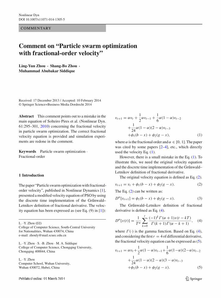
Nonlinear DynDOI 10.1007/s11071-014-1305-5

COMMENTARY

Comment on “Particle swarm optimizationwith fractional-order velocity”

Ling-Yun Zhou · Shang-Bo Zhou ·Muhammad Abubakar Siddique

Received: 17 December 2013 / Accepted: 10 February 2014© Springer Science+Business Media Dordrecht 2014

Abstract This comment points out to a mistake in themain equation of Solteiro Pires et al. (Nonlinear Dyn.61:295–301, 2010) concerning the fractional velocityin particle swarm optimization. The correct fractionalvelocity equation is provided and simulation experi-ments are redone in the comment.

Keywords Particle swarm optimization ·Fractional-order

1 Introduction

The paper “Particle swarm optimization with fractional-order velocity”, published in Nonlinear Dynamics [1],presented a modified velocity equation of PSO by usingthe discrete time implementation of the Grunwald–Letnikov definition of fractional derivative. The veloc-ity equation has been expressed as (see Eq. (9) in [1]):

L. -Y. Zhou (B)College of Computer Science, South-Central Universityfor Nationalities, Wuhan 430074, Chinae-mail: zhouly@mail.scuec.edu.cn

L. -Y. Zhou · S. -B. Zhou · M. A. SiddiqueCollege of Computer Science, Chongqing University,Chongqing 400044, China

L. -Y. ZhouComputer School, Wuhan University,Wuhan 430072, Hubei, China

vt+1 = αvt + 1

2αvt−1 + 1

6α(1 − α)vt−2

+ 1

24α(1 − α)(2 − α)vt−3

+φ1(b − x) + φ2(g − x), (1)

whereα is the fractional order andα ∈ [0, 1]. The paperwas cited by some papers [2–4], etc., which directlyused the velocity Eq. (1).

However, there is a small mistake in the Eq. (1). Toillustrate this, we need the original velocity equationand the discrete time implementation of the Grunwald–Letnikov definition of fractional derivative.

The original velocity equation is defined as Eq. (2).

vt+1 = vt + φ1(b − x) + φ2(g − x). (2)

The Eq. (2) can be written as:

Dα[vt+1] = φ1(b − x) + φ2(g − x). (3)

The Grunwald–Letnikov definition of fractionalderivative is defined as Eq. (4).

Dα[x(t)] = 1

T α

r∑

k=0

(−1)kΓ (α + 1)x(t − kT )

Γ (k + 1)Γ (α − k + 1), (4)

where Γ (·) is the gamma function. Based on Eq. (4),and considering the first r = 4 of differential derivative,the fractional velocity equation can be expressed as (5).

vt+1 = αvt + 1

2α(1 − α)vt−1+ 1

6α(1−α)(2−α)vt−2

+ 1

24α(1 − α)(2 − α)(3 − α)vt−3

+φ1(b − x) + φ2(g − x). (5)

123

L. -Y. Zhou et al.

100 200 300 400 500 600 700 800 900 10000

20

40

60

80

100

120

140

160

180

200

t

Col

ville

alpha=0

alpha=0.3

alpha=0.6alpha=0.9

PSO

100 200 300 400 500 600 700 800 900 10000

0.5

1

1.5

t

Boh

ache

vsky

alpha=0

alpha=0.3

alpha=0.6alpha=0.9

PSO

100 200 300 400 500 600 700 800 900 10000

0.5

1

1.5

t

Eas

om

alpha=0

alpha=0.3

alpha=0.6alpha=0.9

PSO

100 200 300 400 500 600 700 800 900 10000

0.05

0.1

0.15

0.2

0.3

0.35

0.4

0.45

t

alpha=0

alpha=0.3

alpha=0.6alpha=0.9

PSO

Dro

pwav

e

0.25

100 200 300 400 500 600 700 800 900 1000150

200

250

300

350

t

Ras

trig

in

alpha=0

alpha=0.3

alpha=0.6alpha=0.9

PSO

Fig. 1 FOPSO with various values of α on five test functions

The velocity equation (5) shows a little differencewith the velocity equation (1). We regard the PSO withvelocity Equation (5) as FOPSO. If we set α = 1,

then the above Eq. (5) becomes Eq. (2). Therefore, thePSO algorithm is a special case of FOPSO algorithm.Because fractional derivatives have a memory of all the

123

Particle swarm optimization

past events and the influence of past events decreasesover time, it is more suited to describe the dynamicphenomena of particle’s trajectory adequately.

2 Simulation results

To examine the impact of the parameter α on theanytime behavior of PSO with fractional velocity(FOPSO), several tests are developed. The test func-tions in the paper [1] are adopted in the experiments. Ineach experiment where one parameter α is varied, theother parameters are kept fixed at the values as sameas the values of the paper [1]. Our goal is to identifywhich parameter settings produce the best results at anymoment during the algorithm execution. Twenty inde-pendent runs on each function. The curves for eachfunction between the mean value of the function andthe number of iterations are shown in Fig. 1.

It can be seen that the convergence of the algorithmdepends directly upon the fractional order α on all thefunctions. On most of the functions, the SQT curvescross for the different parameter settings and those withsmaller values of α are initially better, but quickly leadto search stagnation. The smaller values more proba-bility result in worse final solution quality. However, a

larger values of α produces much better results towardsthe end of the run. The value 0.9 of α makes the algo-rithm perform better than the other factional order val-ues during most of the search process. The FOPSOwith the value 0.9 of α outperforms standard PSO inthe convergence perspective point of view.

Acknowledgments The work described in this paper was car-ried out with the support of the National Natural Science Foun-dation of China (NSFC) (No. 61103248).

References

1. Solteiro Pires, E.J., Tenreiro Machado, J.A., de MouraOliveira, P.B., Boaventura Cunha, J.: Particle swarm opti-mization with fractional-order velocity. Nonlinear Dyn. 61,295–301 (2010). doi:10.1007/s11071-009-9649-y

2. Couceiro, M.S., Rocha, R.P., Fonseca Ferreira, N.M., Ten-reiro Machado, J.A.: Introducing the fractional-order Dar-winian PSO. Signal Image Video Process. 6, 343–350 (2012)

3. Ghamisi, P., Couceiro, M.S., Benediktsson, J.A.: An efficientmethod for segmentation of images based on fractional calcu-lus and natural selection. Expert Syst. Appl. 39, 12407–12417(2012)

4. Ghamisi, P., Couceiro, M.S.: Multilevel image segmenta-tion based on fractional-order Darwinian particle swarmoptimization. IEEE Trans. Geosci. Remote Sens. 99, 1–13(2013)

123