Combining Symbolic Conflict Recognition With Markov Chains ...
167
Combining Symbolic Conflict Recognition With Markov Chains For Fault Identification 4 Finlay S. Smith V W -11 1, r I N5 Ph.D. University of Edinburgh 2002
Transcript of Combining Symbolic Conflict Recognition With Markov Chains ...

Combining Symbolic Conflict Recognition With Markov
Chains For Fault Identification 4
Finlay S. Smith
V
W-111,
r
I N5
Ph.D.
University of Edinburgh
2002

Abstract
Model based fault diagnosis systems use a conflict recognition technique to detect con-flicts between the observed behaviour of a physical system and its expected behaviour, as well as determining which components faulty behaviour could have led to this dis-crepancy. These conflicts are used to identify possible fault candidates, whose predicted behaviour is compared to the observed behaviour. This process continues until a model is found whose behaviour matches the observed behaviour. The selection of candidates is often based upon the possibility of components failing as well as the conflict sets. In these systems the uncertain evidence from each conflict set is only used to identify possible candidates and not to update the beliefs in possible behaviours.
A novel approach is presented in this thesis that exploits uncertain information on the behavioural description of system components to identify possible fault behaviours in physical systems. The result is a diagnostic system that utilises all available evi-dence at each stage. The approach utilises the standard conflict recognition technique developed in the well-known General Diagnostic Engine framework to support diag-nostic inference, through the production of both rewarding and penalising evidence. The penalising evidence is derived from the conflict sets and the rewarding evidence is derived, in a similar way, from two sets of components both predicting the same value of a given variable within the system model. The rewarding evidence can be used to increase the possibility of a given component being in the actual fault model, whilst penalising evidence is used to reduce the possibility.
Markov matrices are derived from given evidence, thereby enabling the use of Markov Chains in the diagnostic process. Markov Chains are used to determine possible next states of a system based only upon the current state. This idea is adapted so that instead of moving from one state to another the movement is between differ-ent behavioural modes of individual components. The transition probability between states then becomes the possibility of each behaviour being covered in the next model. Markov matrices are therefore used to revise the beliefs in each of the behaviours of each component.
This research has resulted in a technique for identifying candidates for multiple faults that is shown to be very effective. The process was evaluated by intensive testing on a physical system containing a total of ninety components. To illustrate the process, electrical circuits consisting of approximately five hundred components are used to show how the technique works on a large scale. The electrical circuits used are drawn from a standard test set.
11

Acknowledgements
I would like to thank my supervisors Dr. Shen and Dr Ross for their help and support throughout my studies at Edinburgh University. I would especially like to thank all members of the Approximate and Qualitative Reasoning group for their support, help and friendship. In particular, I would like to thank Elias Bins for his help during the early stages of my work and Ian Miguel for helping me with accessing files during the past year when I took up a Lecturship at NUT, Galway.
I would also like to thank the EPSRC for their financial support which allowed me to undertake the PhD and The Department of Transport for giving me the incentive to improve my education.
Thanks are also due to The Department of Information Technology at NUT Galway for facilitating the completion of my thesis.
Special thanks go to my parents for providing moral, financial and practical support, especially over the final twelve months.
Finally, I would like to thank Gillian for her continued support and for putting up with all the difficulties of the last 5 years.
111

Contents
Abstract
Acknowledgements
Declaration
List of Figures
List of Tables
11
I"
iv
ix
x
1 Introduction 1
1.1 Diagnosing Multiple Faults .........................3
1.2 Uncertainty in Fault Diagnosis .......................6
1.3 Diagnosing Faults in Dynamic Systems ...................8
1.4 Structure of the Thesis ............................10
2 Background 12
2.1 Diagnosing Faults in Static Systems ....................12
2.1.1 Assumption-Based Truth Maintenance System ..........13
2.1.2 General Diagnostic Engine .....................13
2.1.3 GDE+ .................................18
2.1.4 Sherlock 19
2.2 Fault Detection and Isolation ........................20
2.3 Al Approaches to Diagnosing Faults in Dynamic Systems ........21
2.4 Approximate Reasoning in Fault Diagnosis ................26
2.5 Markov Chains in Fault Diagnosis .....................29
2.5.1 The Dempster Shafer Theory of Evidence .............29
2.5.2 Markov Chains . . . . . . . . . . . . . . . . . . . . . . . . . . . . 30
2.6 Fuzzy Systems ................................33
2.6.1 Fuzzy Modelling ...........................34
2.6.2 Fuzzy Logic and Neural Networks .................37
3 Markov Chains in Fault Identification 39
3.1 Using Beliefs to Guide Candidate Generation ...............39
3.1.1 Initialise Beliefs ............................40
3.1.2 Select a System Model ........................41
3.1.3 Detect Conflicts in the Model ....................43
3.1.4 If Conflicts Exist ............................43
3.1.5 Else ..................................46
3.1.6 Re-initialise Beliefs ..........................46
3.1.7 Go to Step 2 .............................46
3.1.8 Terminating the Algorithm .....................47
3.2 Using Markov Chains to Revise Beliefs ...................47
4 Markov Chains-Aided Candidate Generation 50
4.1 Deriving the Markov Matrices . . . . . . . . . . . . . . . . . . . . . . . 50
vi

4.2 Generalisation . 54
4.3 Dealing with More than One Piece of Evidence ..............62
4.3.1 Illustrative Example .........................63
4.3.2 Overview of the Process to Combine Beliefs ............63
4.3.3 Combining Individual Pieces of Evidence .............67
4.4 Creating the Markov Matrices . . . . . . . . . . . . . . . . . . . . . . . . 72
4.5 Combining the Markov Matrices . . . . . . . . . . . . . . . . . . . . . . 74
5 Comparison with Existing Static Techniques 78
5.1 The System under Diagnosis ........................79
5.2 Markov Chains for Belief Revision ......................79
5.3 GDE+ .....................................82
5.4 Sherlock ....................................84
5.5 Summary ...................................85
6 Experimental Evaluation of the Approach
86
6.1 The System under Diagnosis ........................86
6.1.1 Behavioural Fragments for Each Component ...........87
6.2 Experimental Methodology .........................91
6.3 Results .....................................91
6.3.1 The Number of Models Simulated .................92
6.3.2 Single Fault Solutions ........................94
6.3.3 The Prior Certainties of Simulated Models ............96
6.4 Discussion ...................................97
7 Finding Faults in an ISCAS '85 System: An Application Study 101
vii

7.1 The System under Diagnosis . 101
7.1.1 Components in the Model ......................102
7.1.2 Behavioural Fragments for Each Component ...........103
7.2 Results .....................................103
7.2.1 First Result - Possible Single Fault ................104
7.2.2 Second Result - Double Fault ....................105
7.2.3 Third Result - Another Double Fault ................108
7.3 Discussion ...................................110
8 Conclusions and Future Work
113
8.1 Future Work .................................115
8.1.1 Diagnosing Static Systems ......................116
8.1.2 Extending to the Diagnosis of Faults in Dynamic Systems . . 118
8.1.3 Application of Ideas to Other Fields ................121
Bibliography 122
A Proofs 132
B The Model Analysed in Detail 142
C The Model of the ISCAS '85 System Under Diagnosis 146
viii

List of Figures
1.1 A Simple One Tank Example 4
1.2 A Simple Heated One Tank Example ...................5
2.1 Illustrative Diagnostic Problem .......................14
2.2 Model Based Diagnosis of Continuous Systems ..............23
3.1 Key Stages of the Diagnostic Algorithm ..................41
4.1 Combining Pieces of Evidence .......................64
5.1 Illustrative Diagnostic Problem .......................80
6.1 Low Level Detail of the System Under Diagnosis .............87
6.2 Level 1 of the System Under Diagnosis ..................88
6.3 Level 2 of the System Under Diagnosis ..................89
6.4 Summarised results .............................94
6.5 Summarised results where the faults do not interact ...........95
6.6 Summarised results where the faults do interact ..............96
7.1 Two Faults Reflected Though Single Candidate .............110
ix

List of Tables
2.1 Using DST to Combine Evidence . 30
5.1 The Evidence Generated ..........................81
5.2 The Revised Beliefs .............................81
6.1 The Number of Models Simulated for each Test .............93
6.2 The Results of Test 8 .............................97
6.3 The Results of Test 5 .............................98
6.4 The Results of Test 37 ............................98
6.5 The Results of Test 100 ...........................99
6.6 The Results of the Revised Test 37 .....................99
6.7 The Results of the Revised Test 100 ....................100
7.1 The Results of the First Test ........................104
7.2 The Results of the Second Test .......................106
7.3 The Results of the Third Test .......................109
x

Chapter 1
Introduction
The problem of diagnosing faults in physical systems is a difficult one, both for human
experts and for automated processes. Traditional methods of fault diagnosis require
'experts' whose understanding of the physical system is based upon a vast techni-
cal knowledge and often previous experience at diagnosing faults in the same system.
Early attempts at automated diagnosis [Buchanan & Shortliffe 84] often relied upon
this same knowledge. In particular if a previously unknown fault occurred the system
would be unable to diagnose the correct fault and may even suggest several erroneous
possibilities. Model based diagnosis overcomes these problems by modelling the inter-
nal structure of a physical system, and thus having the ability to predict behaviours,
and in particular deal with previously unknown faults [Haxnscher et al. 92].
A related problem is that of fault detection: a process of detecting the existence of a
fault in a system without having to say what the fault is. The standard method for
detecting faults in physical systems is to have a model of the way the system is expected
to behave. This model can be anything from a detailed numerical representation of the
physical system, through to qualitative representations [Kuipers 941 and the model is
simulated (using a suitable simulator) generating an expected behaviour of the physical
system. This expected behaviour is then compared to the actual observed behaviour,
with any discrepancies indicating that a fault has occurred. This process is repeated
continuously, reporting either no discrepancies (therefore no faults) or discrepancies
(therefore faults). Once discrepancies have been detected the fault diagnostic process
1

CHAPTER 1. INTRODUCTION 2
is initiated.
The detection of discrepancies themselves can sometimes be difficult, for example using
a numerical model it is almost impossible to exactly predict the actual behaviour as
there will always be errors (due to noise, model deficiencies etc.). One solution to this
problem would be to allow for small discrepancies between the predicted value and the
observed value, however this is also problematic as small faults may go undetected for
some time (consider a slight leak in a pipe).
When diagnosing faults there are two most important issues requiring consideration;
one being are the accuracy of the diagnosis and the other being the speed at which the
diagnosis is made. If the diagnosis is not accurate, not only will the system continue
to display faulty behaviour, but the unnecessary repairs could have been expensive in
terms of parts and labour (whilst the machine is being repaired it is out of service and
therefore not performing its function). Similarly a fast diagnosis is important, if the
diagnosis takes a relatively long time there are two significant areas where this could
prove problematic. If the system is shut down whilst a diagnosis takes place, a long
delay could result in a great deal of lost production for a, possibly, minor fault. On
the other hand some systems (e.g. power stations) can take a long time to stop and
then restart, and so it is often desirable to diagnose the fault before deciding whether
or not to stop the process. In this situation a fast diagnosis is essential as the fault
may be a serious one that could lead to further damage to the system.
The reliance on the existence of expertise is particularly problematic for new systems,
where the expertise may not yet exist (or is only very limited). The ability to diagnose
faults without detailed knowledge of potential faults would obviously be extremely
beneficial.
The aim of automated fault diagnosis is therefore to bring all of these strands together
to create a diagnostic process that is fast, accurate and not completely dependant on
detailed knowledge of the physical system.

CHAPTER 1. INTRODUCTION
3
1.1 Diagnosing Multiple Faults
The simplest forms of diagnosis assume that only one fault occurs at a given time. The
aim in such systems is to find the single fault that would have caused the discrepancies.
The problem with this approach is that it is common for more than one fault to occur
at a time, for example in an electrical circuit, a power surge may damage several
components. In such situations a diagnostic process that cannot deal with multiple
faults could be almost useless, and indeed may attempt to diagnose completely different
faults.
The diagnosis of multiple faults that jointly occur is far more complex than the diag-
nosis of single faults. Apart from the possible increase in the number of discrepancies
there are potentially more subtle problems.
In the simplest possible case there could be two separate faults each of which displays
its own distinct set of discrepancies. As there is no overlap between these two sets of
discrepancies a simple extension to a single fault diagnostic process should be able to
diagnose these two faults. Similarly, if more than two such faults occurred they could
be diagnosed. A rule-based diagnostic system that had separate rules for each possible
fault would be an ideal choice for such a diagnostic system [Buchanan & Shortliffe 84]
as it would easily move from diagnosing single faults to diagnosing multiple faults.
Unfortunately multiple faults in physical systems are rarely as easy to diagnose as this.
Multiple faults in a physical system can often interact with each other, so that instead
of displaying a simple conjunction of the separate discrepancies, a completely different
set of discrepancies can be generated.
Several possible effects can occur. Firstly, the discrepancies can re-enforce each other,
for example consider the simple system in figure 1.1. Two possible faults are that
the pipe IN is allowing more liquid into the tank and that the pipe OUT is partially
blocked. In both cases the result is that the height in the tank will rise. If both faults
occur together the height of liquid in the tank will increase by an even greater amount.
As a result a simple diagnostic system would be unable to diagnose the two faults.
Secondly, the discrepancies can partially (or even completely) cancel each other out.

CHAPTER 1. INTRODUCTION
4
IN
- -if
Figure 1.1: A Simple One Tank Example
Again using the system in figure 1.1 to illustrate this, consider the following two faults,
a partial block in the pipe IN and a partial block in the pipe OUT. The first of these
two faults would result in a reduction in the height of the liquid in the tank, whilst
the second would result in an increase in the height of the liquid in the tank. If both
of these faults occurred simultaneously the effect on the height of the liquid would be
reduced (compared to the two individual faults) with the exact value being dependant
on the scale of the two blockages. Again a simple diagnostic process would be unable
to diagnose these two faults (especially if the effects of the two faults almost cancel
each other).
Finally, the two faults could combine to create a completely separate discrepancy that
does not occur when either of the single faults occur on their own. To illustrate this
situation consider the system in figure 1.2, in this example the liquid could be molten
steel. Again if the flow through pipe IN dropped the height of the liquid in the tank
would drop and consequently so would the flow through pipe OUT. If the heating
system failed the liquid would cool and so the liquid steel would cool slightly. However
if the two faults occurred simultaneously the effect could be that the height of the liquid
would fall, with the subsequent reduction in flow causing the steel to cool sufficiently
(especially when the loss of heat is considered) so that it blocked the pipe. In this case
neither single fault on its own would cause the blockage. A simple diagnostic system
would therefore be unable to diagnose either of these two faults.

CHAPTER 1. INTRODUCTION
5
IN
if
HEAT SOU RCE
Figure 1.2: A Simple Heated One Tank Example
A simplistic approach to solving this problem would be to extend the definition of a
single fault so that all possible combinations of single faults can be defined as a special
case of a 'single fault'. In this way the simple rule based diagnostic processes could
easily be extended to cover multiple faults. There are however two major problems
with this approach.
Firstly, it is unlikely that all possible multiple combinations of faults have occurred in
a particular system. In this case either exact rules for each combination could not be
created (in which case only faults that have occurred previously could be diagnosed)
or all possible fault combinations would have to be engineered into the system and the
consequent fault behaviours recorded. This approach may not only involve a major
effort in terms of time but may also be dangerous and expensive when dealing with
serious faults. For this approach to work every possible combination would need to
be determined before hand, greatly increasing the complexity of the diagnostic process
and hence likely to greatly reduce the speed of the simple diagnoses.
Secondly and more fundamentally, the number of multiple faults is likely to be very
large. Even for a simple situation where a component is either faulty or not faulty and
with only 10 components in the system, the number of potential multiple faults is 2'0 =
1024. To have more than a thousand faults for such a simple system makes the resultant

CHAPTER 1. INTRODUCTION 6
diagnostic process very complex. If the process is then to be scaled up to a slightly
more realistic problem say with 20 components (again with only the two behaviours)
the number of potential multiple faults becomes 220 = 1048576, so even this relatively
simple problem would require knowledge of over a million fault combinations. Clearly
when this is scaled up, both in terms of the number of components and the number of
possible behaviours of each component, the problem very quickly becomes intractable.
Thus an approach is required that is not dependant on the prior knowledge of all
possible combinations of faults, though knowledge of the localised effect of individual
faults could be very useful.
1.2 Uncertainty in Fault Diagnosis
The examples in the previous section mainly considered diagnostic problems where
components are either not faulty or faulty with no distinct fault behaviours. In general
there may be some known ways in which components may fail and these known faults
can then be modelled. Such information can be very useful in performing automated
fault diagnosis.
A simple example of this would be a pipe similar to those used in the previous section,
the pipe may be non-blocked (normal behaviour), partially blocked, completely blocked
or even leaking (with various degrees of blockage or leakage). Each of these possible
behaviours could then be modelled as a possible fault behaviour for that component.
In addition, as it is unlikely that all possible fault behaviours of the components are
known an additional possibility is that the component is behaving in some unknown
manner. An additional potential behaviour must therefore be allowed for so that the
diagnostic system can diagnose an unknown fault in a component.
This increase in the number of possible behaviours obviously increases the complexity
of the diagnostic problem, as the number of potential models increases exponentially.
Certain components are more likely to have faults than others (e.g. some components
may be more reliable or suffer from less wear). Also within each component some
of the behaviours are more likely than others (specifically the normal behaviour of a
component is its most likely state). If a reasonable number of behaviours are known

CHAPTER 1. INTRODUCTION 7
it is also reasonable to assume that the component is more likely to behave in one of
the known ways than in some unknown way. This assumption also aids the diagnostic
process as less likely behaviours are not considered until the more likely ones have been
ruled out, thus the diagnostic systems will not consider some unknown behaviour until
the known behaviours have been eliminated.
To handle this range of likelihoods each of the possible behaviours of a component
may be assigned a belief. These beliefs reflect the likelihood of each of the behaviours
representing the observed behaviour in the physical system. These beliefs can be based
upon probabilities (e.g. for Bayesian inference [Pearl 88, Pearl 01]) or may just give
an indication of which behaviours are more likely than others. These beliefs can then
be used to suggest candidates to explain the faults which can be tested or evaluated.
The use of probabilities may be problematic. The derivation of exact probabilities
can be very difficult, especially if there is little existing evidence from the failure of
components. In addition the propagation of probabilities can be rather complex.
The use of beliefs presented here is based upon the assumption that little is known
about the likelihood of individual components failing (and if it does fail, the probabil-
ities of it failing in each way). The work presented in this thesis assumes that each of
the known fault behaviours are as likely as each other, with the unknown behaviour
belief being lower and the normal behaviour belief being higher. However, if some
knowledge is available about which components are more likely to fail, this can be
incorporated by adjusting the initial beliefs. This would enhance the performance of
the diagnosis as more 'believed' models would be checked sooner.
The work on the handling of uncertainty presented here combines the diagnosis of
multiple faults with the use of beliefs to help guide the search for fault candidates
(models that explain the observed discrepancies and could therefore be candidates for
explaining the faults). The process combines symbolic conflict recognition from GDE
[deKleer & Williams 87] with Markov Chains to produce a process for fault identifica-
tion. The initial beliefs are set arbitrarily and are continually revised using evidence
in the form of conflict and confirm sets generated during the diagnostic process for
and against components. Conflict sets are groups of components whose combined be-

CHAPTER 1. INTRODUCTION 8
haviour produces a conflict (two different values for the same variable). Confirm sets
are groups of components whose combined behaviour generates the same value for a
given variable in more than one way. In addition the conflict sets are recorded so that
a known set of conflicts are never tried again. The model that is most believed (as
long as it does not contain any of the conflict sets) is then selected and simulated.
The result is then compared against the observed behaviour, if conflicts still exist the
conflict and confirm sets are revised to enable the beliefs to be generated and another
model selected. This process continues until a model is found that does not display
any discrepancies (with respect to the observed behaviour) at which point the process
is either terminated or further possible candidate models can be searched for.
The result is a process that not only uses the beliefs in each of the fragments, but that
also revises them based upon evidence generated during the diagnostic process. The
results from implementations of this novel model-based inference process show that the
process very quickly finds fault candidates, even in fairly sizeable physical systems.
1.3 Diagnosing Faults in Dynamic Systems
The initial work outlined in the previous section illustrated the techniques on static
systems. Static systems are easier to diagnose than dynamic ones. In static systems,
for a fixed set of inputs, the outputs never change. Therefore it is relatively easy to
diagnose faults. In dynamic systems, however, the outputs can constantly change with
time, often with 'feedback' loops that cause future states to be dependant, not only on
the current inputs to the system, but also to some previous input and output.
A significant problem with dynamic systems is the progression of the behaviour of
the system with respect to time. In static systems the simulation process is relatively
straightforward, but in dynamic systems the simulation needs to be continually per-
formed to simulate the behaviour of the system over time. This reliance on time poses
several problems for the diagnostic process. If the fault is fairly minor, for example a
very small leak in a pipe, it may take a considerable period of time before the fault
can be detected (i.e. until the discrepancies are significant enough) and then it will
not be obvious whether the fault was a small long standing leak or a newer relatively

CHAPTER 1. INTRODUCTION
9
large one.
Recent work at NASA has led to model based diagnosis, amongst other Al techniques
being developed as part of NASA's unmanned probe program [Muscettola et al. 98].
For such systems reliability robustness and flexibility are essential properties, as,
though the probes can be controlled remotely from mission control, the time delay
between the probe sending a signal and receiving a reply can be significant and could
affect the probe's ability to survive.
A fundamental time related problem is that the temporal behaviour of the model
has to be matched against the observed behaviour with various associated problems
such as when did the fault occur and matching modelled 'snapshots' against observed
'snapshots'. These matching problems significantly increase the complexity of the
diagnostic problem.
As the diagnosis progresses more time will pass and so the length of each simulation
must increase (as more states will have to be modelled, slowing down the process).
Numerical simulations can be very complex and precise, but their complexity and
the difficulty in obtaining them makes them a poor choice when considering dynamic
diagnosis. A more appropriate simulation method is qualitative simulation [Kuipers 94]
which only considers trends in the behaviour rather than actual numerical values and
hence theoretically is more suited to diagnosis.
The work on diagnosis of faults in dynamic systems presented in this thesis falls into
two distinct areas. Firstly the belief revision process that was used on the static systems
is extended to dynamic systems. The result is a process that effectively selects models
for simulation, based upon the observed discrepancies in all of the models simulated
previously in an attempt to find candidates by checking as few models as possible.
The initial results from this work suggest that the approach should be as effective in
dynamic diagnosis as the earlier work was in static diagnosis.
This work is then extended to introduce the concept of a Diagnostic Strategist, a meta-
level guidance tool for controlling the diagnostic process. The Diagnostic Strategist
effectively learns how to guide the diagnosis of faults, with the learning process con-
tinuing over many individual diagnoses to enable future attempts at diagnosis to learn

CHAPTER 1. INTRODUCTION 10
from the mistakes (and successes) of previous diagnoses. This approach enables each
application of the diagnostic process to individually adapt to the peculiarities of the
particular system it is diagnosing faults in.
Most of the work described in this thesis has been presented at most relevant and fore-
most international conferences. A list of published papers is given in the bibliography.
1.4 Structure of the Thesis
An overall structure of the thesis is presented here to give an overview of the key
aspects of the thesis.
The first chapter introduces the key points and concepts of the thesis. The main
justifications for the work carried out and the key results are presented in outline
forming a brief summary of the contents of the thesis. This chapter outlines some
of the difficulties in diagnosing multiple faults and in diagnosing faults in dynamic
systems.
The second chapter provides a background discussion on the major themes of the the-
sis. Each of the major topics are described with particular emphasis being given to the
advantages of each technique and any limitations that will need to be overcome. As
some of the topics have considerable literature published on them the major focus of the
discussion is on work relating to fault diagnosis, though the major work in each of the
fields is considered. The major topics considered are fault diagnosis (GDE (General Di-
agnostic Engine) type systems [Forbus & deKleer 94, Struss & Dressler 89], dynamic
diagnosis [Dvorak & Kuipers 89, Dvorak & Kuipers 91], Bayesian networks in diagno-
sis [Leung & Romagnoli 00, Won & Modarres 98, Chen & Srihari 94], Markov chains
in diagnosis and fuzzy logic in diagnosis [Smith & Shen 98b, Linkens & Chen 99]),
self-organising fuzzy logic controllers [Procyk & Mamdani 79, Patrikar & Provence 93,
Lin & Lin 95, deBruin & Roffel 96], the Dempster Schafer theory of evidence (DST)
[Shafer 76] and the Assumption-based Truth Maintenance System (ATMS) [deKleer 86a,
Forbus & deKleer 94].
Chapters three and four describe the application of Markov chains [Stewart 94] to fault

CHAPTER 1. INTRODUCTION 11
diagnosis in a GDE type environment. Chapter 3 develops the use of Markov Chains
in belief revision and outlines the overall process and presents the basic ideas behind
the research presented in this thesis.
Chapter four formalises the use of Markov chains to revise the beliefs in model frag-
ments. The method for generating the Markov chains and are developed and justified.
Illustrative examples are used to demonstrate the novel ideas. Proofs to the key the-
ories are presented in Appendix A. This chapter includes a description of the fuzzy
DST which is an extension of the DST, so that the presentation is self-contained.
Chapter five compares the approach developed through the use of Markov chains with
other relevant diagnostic techniques by the use of a common illustrative example. Both
the performance of each technique and an analysis of the complexity of each technique
is presented.
The next chapter details a rigorous testing the approach on a reasonably complex
model, with a significant number of tests. A potential limitation of the approach is
identified and a solution is proposed.
The penultimate chapter demonstrates the scalability of the techniques developed by
applying them to a considerably larger system. It illustrates not only that the tech-
nique effectively generates fault candidates in an efficient manner, but that the process
does not suffer from complexity problems. The techniques are applied to a standard
electrical circuit which contains more than 500 components.
The final chapter brings all of the work together and draws overall conclusions. Each of
the techniques and their applications are analysed and any shortcomings are identified.
Ideas for extending the existing work and related applications are then discussed.

Chapter 2
Background
This chapter is a discussion on related work in the diagnosis of faults in physical
systems. It is organised in several sections, each of which considers a different approach
to fault diagnosis. As each of these sections addresses diagnostic systems based upon
widely differing techniques, the basics of each of these techniques will also be discussed.
The first section will discuss the range of diagnostic approaches that have been de-
veloped, based largely upon the original work as reported in [deKleer & Williams 87].
The diagnostic work on static systems presented in this thesis are derived from this
work, so considerable discussion of this area will be presented. The second section will
look at the diagnosis of faults in dynamic systems. The third and fourth sections will
examine the role of Bayesian and Markovian approaches to fault diagnosis respectively.
The final section will discuss the role of fuzzy logic in the diagnosis of faults in physical
systems.
2.1 Diagnosing Faults in Static Systems
The diagnosis of faults in static systems has been the subject of much work over
recent years [deKleer & Williams 87, deKleer & Williams 89, deKleer 91, Struss 92,
Forbus & deKleer 94, Lee & Kim 93, Nooteboom & Leemeijer 93, Fattah & Dechter 95,
Dressler & Struss 96, Lucas 98, Mauss & Sachenbacher 991.
12

CHAPTER 2. BACKGROUND 13
2.1.1 Assumption-Based Truth Maintenance System
The basis for much of this work is the Assumption-based Truth Maintenance System
(ATMS) [deKleer 86a, deKleer 86b, deKleer 86c, Forbus & deKleer 94]. The ATMS
efficiently records all possible explanations for an observed behaviour, by keeping track
of the reasoning process through the use of assumption sets. In fault diagnosis, the
assumptions are that a given component is behaving in a given way. These assumption
sets record every way that a given value can be derived.
A major factor in gaining the efficiency in reasoning with these assumption sets is that
they only record the minimal sets needed to reach a given conclusion. This simplifica-
tion significantly reduces the number of different assumptions to be recorded, without
the loss of any generality, as these sets represent the least amount of information to
reach the given conclusion.
Crucially, the ATMS allows multiple solutions to be generated simultaneously, which
makes it very attractive for diagnosing multiple faults in a physical system. The ability
to generate multiple candidates, and generally to focus on those minimal candidates
(those candidates with the fewest faulty components) is ideally suited to fault diagnosis.
Multiple candidates need to be explored before settling on a diagnosis and checking
minimal faults first is a reasonable method as generally a few faulty components are
more likely than many faulty components.
2.1.2 General Diagnostic Engine
The use of ATMS led to the development of a landmark in model based diagnosis, the
General Diagnostic Engine (GDE) [deKleer & Williams 87]. This diagnostic program
uses the ATMS to record how predicted values were derived, which allowed GDE
to easily suggest multiple (and minimal) fault candidates. GDE is used to diagnose
multiple faults in static electrical circuits (though applications of GDE to other domains
have also been reported [deKoning et al. 00]). Figure 2.1 shows an example of a simple
circuit, which will be used to illustrate the method used in the GDE.
GDE makes several assumptions, firstly that it is known that a fault occurs, secondly

CHAPTER 2. BACKGROUND
14
=2
3=8
Figure 2.1: Illustrative Diagnostic Problem
that multiple faults can occur, thirdly that the model represents the physical system
and finally that a component either works or it does not (that is there are no fault
models). GDE also assumes that faults must occur in components, which is not as
limiting as it first appears as wires can also be represented as simple components.
Additionally GDE assumes that the faults are non-intermittent and are not dynamic.
The method employed by GDE is to use the known values, generally the inputs (A, B,
C, D and E in figure 2.1) and outputs (F and G in figure 2.1) to propagate through the
model allowing predicted values to be generated for each of the internal variables (X, Y
and Z in figure 2.1). In figure 2. 1, components Al and A2 are adders (the output is the
sum of the two inputs) and components Ml, M2 and M3 are multipliers (the output
is the product of the tvo inputs). Whenever two different values are predicted for
the same variable a conflict exists, and as a variable cannot have two different values
simultaneously a conflict therefore exists. Further, as it is known how the two values
were derived, at least one of the components that was used to predict either of the
two values must be faulty. The combination of the two sets of components that led to
the derivation of conflicting values is called a conflict set. Once all the propagations
have occurred, sets of possible candidates can be derived by ensuring that each of them

CHAPTER 2. BACKGROUND 15
contains at least one member from each of the conflict sets.
The use of the ATMS and, in particular, its minimal conflict sets greatly reduces
the amount of propagation required, as any predicted values that are derived from
'supersets' of other predicted values are ignored. A set A is a superset of set B if set
A contains at least every member of set B. If set A is a superset of set B, then set B
is a subset of set A.
To illustrate GDE, the example shown in figure 2.1 will be examined. From figure 2.1
the following values are given:
A=3{},B=2{},C=2{},D=3{},E=3{},F=2{},G=8{}
The curly brackets denote, in general, labels that contain the set of assumptions, each
signalling a component to be working correctly, that were used to derive the values.
As all of these values are observed values, they are not derived from the behaviour of
any component in the physical system and so the sets are empty. For such a simple
example it is obvious that the values of F and G should both be 12, so therefore there
must be faults within the physical system. No single fault can explain both F and G
have erroneous values.
These values are now propagated, through the model giving the following values (only
the minimal sets are recorded and therefore shown):
X = 6 {M1}, Y = 6 {M2}, Z = 6 {M3}, X = —4 {A1, M21, Y = —4 {A1, M11
Y = 2 {M3, A21, X = 0 {M3, A2, All, Z = 2 {M2, A21, Z = 12 {A1, MI, A21
The first of these, X = 6 {M1} was derived using the observed values of A and C
and the component Ml (hence the value in the label). Note that the results are not
necessarily presented in the order given here.

CHAPTER 2. BACKGROUND
16
From these predicted values, it is clear that several conflicts exist, namely:
X = 6 {M1},
X = 6 {M1},
X = -4 {A1, M21,
Y = 6 {M2},
Y = 6 {M2},
Y = -4 {A1, M1},
Z = 6 {M3},
Z = 6 {M3},
Z = 2 {M2, A21,
X = -4 {A1, M21
X = 0 {M3, A2, All
X = 0 {M3, A2, All
Y = -4 {A1, M1}
Y = 2 {M3, A21
V = 2 {M3, A2}
Z = 2 {M2, A2}
Z = 12 {A1, MI, A21
Z = 12 {A1, MI, A21
In each of these pairs of predictions both of the values cannot be correct at the same
time and so the union of each pair of sets must contain at least one faulty component.
These set unions are the conflict sets and are as follows:
Al, M21
{M1, M3, A2, All
{Ai, M2, M3, A2, All SUPERSET
Al, Mi} DUPLICATE
{M2, M3, A21
{Ai, Ml, M3, A21 DUPLICATE
M2, A21 DUPLICATE
{M3, Al, Ml, A21 DUPLICATE
{M2, A2, Al, MI, A2} SUPERSET
Four of these sets are just duplicates of other sets and two others have another as a
subset (hence they are not a minimal set). The remaining three minimal conflict sets
are then recorded and used to determine the fault candidates. The details of GDE

CHAPTER 2. BACKGROUND 17
described so far are the conflict recogniser, GDE has detected all of the conflicts and
so fault candidates can now be generated.
As each of these conflict sets must contain at least one component that is faulty, the
fault candidates are sets of components that contain at least one component from each
conflict set. Given the remaining minimal conflict sets:
Al, M21
{M1, M3, A2, All
M3, A21
the minimal candidate sets are:
{M.1, M21 {M1, M31 {M1, A21 {A1, M21
{A1, M31 {A1, A21 {M2, M31 {M2, A21
There are therefore eight minimal candidates, each of which could explain the ob-
served abnormal behaviour of the physical system. Without further information, it
is impossible to select the most likely candidate. GDE can be used to select an ad-
ditional measurement based upon minimum entropy [Shannon 48], that is it tries to
choose a measurement that is most likely to discriminate between the various fault
candidates. This aspect of GDE is not used in the work in this thesis as taking further
measurements increases the diagnostic cost and so it is not considered any further.
The major limiting factor with the original GDE is that it only considered models that
were either working normally or not working normally. This can lead to obviously
inappropriate candidate sets. For example consider a simple system of a battery and
three light bulbs [S truss & Dressler 89], where one bulb is lit and the other two bulbs
are not. The obvious faults here are that the two bulbs that are not lit are broken.
However GDE comes up with 22 minimal candidates including the obvious one. It also
suggests patently ludicrous candidates such as the battery and the bulb that is lit are
both broken, the implication being that the bulb lights up without electricity and is
therefore faulty.

CHAPTER 2. BACKGROUND 18
This limitation of GDE was part of the motivation behind several of the improvements
that were made to GDE [Struss & Dressier 89, deKleer & Williams 89, deKleer 91,
Hamscher et al. 92]. The other main motivation behind these improvements to GDE
was that, in general, some possible known fault behaviours exist. The aim of these
extensions was to combine these known fault behaviours with the relative simplicity
and power of GDE to create more effective diagnostic processes.
2.1.3 GDE+
One such improvement to GDE was called GDE+ [Struss & Dressler 89]. The aim
of GDE+ was to use fault behaviours to determine not only which components were
faulty but also, exactly how they were behaving. GDE+ had the underlying assump-
tion that all possible fault behaviours would be known, and that to determine whether
a component was faulty or not required the testing of all of the possible behaviours.
The principle behind GDE+ was: "If each of the known possible failures of a compo-
nent contradicts the observations, then it is not faulty". So in order to show that a
component was not faulty, each of the possible fault behaviours had to be shown to be
contradictory.
This involves a considerable effort, trying the various combinations of components,
which is a major weakness in the approach. A more fundamental problem with this
approach is the assumption that all possible fault behaviours must be given. This is
often impossible as there may be previously unencountered faults that occur. Following
this approach, if an unknown fault occurs all the known faults may be exonerated
and the component may be wrongly supposed to be working correctly. Even if it
were possible to determine all of the possible fault behaviours of a component, the
potentially large number of them makes their determination and indeed the diagnostic
process itself extremely expensive (in terms of time and effort) as the search space will
grow exponentially.

CHAPTER 2. BACKGROUND
19
2.1.4 Sherlock
Another extension to GDE called Sherlock [deKleer & Williams 89, deKleer 91], de-
rives its name and its motivation from a quote attributed Sherlock Holmes in the novel
"The Sign of the Four": "When you have eliminated the impossible, whatever remains,
however improbable, must be the truth".
Rather than trying to rule out fault behaviours, Sherlock attempts to rule out all known
behaviours, including the normal behaviour. This leads to the possible situation where
all of the possible behaviours of a component have been eliminated. Sherlock handles
this by adding a new kind of behaviour, the unknown behaviour. If all of the other
possible behaviours have been eliminated Sherlock deduces that the component must
be behaving in some previously unknown manner. This additional behaviour allows
Sherlock to avoid having to know all of the possible fault behaviours of a given compo-
nent, rather Sherlock only needs to know the most likely fault behaviours. This greatly
reduces the search space as only a relatively small number of possible behaviours need
to be specified. A problem that Sherlock addresses is that of focussing the diagnosis,
that is determining where the faults are likely to be and then concentrating on those
particular components. This has the advantage of significantly reducing the search
space as Sherlock is only interested in those components that may be faulty.
Another feature that Sherlock uses is that of failure probabilities. Each possible be-
haviour
e
haviour (including the normal behaviour and the unknown behaviour) is assigned an
initial probability. These probabilities are used to select fault candidates. The proba-
bilities are revised based upon the observed values, this has the effect of focussing the
search process to the components in the model that are most likely to be faulty (based
upon the detected discrepancies). The probabilities for normal behaviour are set rel-
atively high (as a component should be more likely to behave normally than display
a fault behaviour. Similarly, the probability associated with the unknown behaviour
is set relatively low (as unknown behaviours are assumed to be unlikely), this has the
additional advantage that the unknown behaviour is only considered after all of the
other behaviours have been considered. The known fault behaviours, can either reflect
the actual probability of the component failing, or can be set to an arbitrary value (the

CHAPTER 2. BACKGROUND
sum of the probabilities must of course come to 1).
When Sherlock generates conflict sets, it uses them to guide the search process by
adjusting the probabilities and then disposing of them. This information on conflicting
observations and predictions is never used again, even though it may contain useful
information.
In a similar piece of work [Nooteboom & Leemeijer 93], the aim is to focus on the most
likely candidates and effectively ignore all of the other components. One of the costs
in this piece of work is that, although the system can focus effectively on certain parts
of the model, all of the inputs and outputs to a particular part have to be measured
together to allow the diagnosis to continue. This is an effect of the focussing, as failing
to measure all of the values could lead to erroneous diagnoses.
A different approach is to use heuristics to guide the diagnostic process [Lee & Kim 93].
The use of heuristics in helping to select measuring points is used in this approach to
improve the performance of the overall diagnostic process. Whilst the results are
promising, the use of heuristics reduces the generality of the diagnostic algorithm and
so limits its use to those physical systems where such heuristic information is available.
The whole aim of model based diagnosis was to move to general diagnostic algorithms
that do not require such heuristic knowledge, and so the introduction of heuristics into
a model based diagnosis reduces the theoretical purity of the program.
2.2 Fault Detection and Isolation
The field of Fault Detection and Isolation (FDI) originated in the control community,
applying statistical and stochastic techniques to the detection and isolation of faults in
physical systems [Chen & Patton 99, Frank et al. 00]. Initially the work concentrated
on static and dynamic systems, though there has been movement towards more com-
plex, non-linear systems. Recently the field has expanded to include contributions from
the Computer Science and Al communities (see the Proceedings of recent Safeprocess
conferences for examples). This expansion has moved the focus of FDI away from
purely Engineering approaches towards Computational Intelligence techniques such as
Qualitative models, Fuzzy logic and Neural Networks.

CHAPTER 2. BACKGROUND 21
One way of detecting faults in physical systems is through the use of hardware re-
dundancy [Frank et al. 99, Mangoubi & Edelmayer 00] where many measurements are
made on a physical system and used to detect faults. However this approach is not
always practical. It may be physically impossible to make all of the required mea-
surements or the inclusion of enough sensors to allow accurate detection may make
the physical system impractical (in terms of weight, volume or cost). As a result of
these limitations the use of models (either quantitative or qualitative) to simulate the
behaviour of the physical system has developed. The discrepancies between observed
behaviour and the behaviour predicted by the model is then used to detect faults.
The approach is similar to that used in Model Based Reasoning in the field of AT and
therefore to the work presented in this thesis.
The problem with such an approach is that exact models of physical systems are
difficult (if not impossible) to formulate, giving rise to uncertainty in the predicted
behaviours. This uncertainty can be handled by relaxing the assumption that predicted
and observed values should exactly match, however this can lead to further problems.
For example, if the tolerance level is set too low many false alarms may occur. On
the other hand if the tolerance is set to high faults may not be detected. The work
presented in this thesis assumes that faults have already been detected and then alms
to identify the actual faults, it is therefore not affected by the problem of setting a
tolerance level.
The problem of minimising false alarms, whilst detecting faults is of particular im-
portance in fault tolerant control [Blanke et al. 97]. In fault tolerant control, the aim
is to minimise the frequency of plant shut downs, whilst minimising the risk of not
detecting faults. The balance required in fault tolerant control is similar to that in
fault detection.
2.3 Al Approaches to Diagnosing Faults in Dynamic Sys-
tems
Processes for diagnosing faults in static systems are at a fairly advanced stage, how-
ever many physical systems are not static and have at least an element of dynamic be-

CHAPTER 2. BACKGROUND 22
haviour, in extreme all physical systems are in fact dynamic. There are existing systems
for diagnosing faults in dynamic systems [Dvorak & Kuipers 89, Dvorak & Kuipers 91,
Rayudu et al. 95, Bottcher 95, Puma & Yamaguchi 95, Guan & Graham 96, Larsson 96,
Frank & Koppen-Seliger 97, Struss et al. 97, Chantler et al. 98], but they are not as
well developed as those for static systems.
The major difficulty with diagnosing faults in dynamic systems is the very dynamic
nature of them. In static systems, as the values never change it is relatively easy to
find a model that explains the observed behaviour. In dynamic systems, however, time
makes the dynamic process considerably more complex.
A fundamental difficulty rests even in detecting that discrepancies exist. As the physi-
cal system behaviour varies over time, it becomes a problem just to match the predicted
behaviour against the observed behaviour which is necessary if any discrepancies are
going to be detected. This can create problems, especially if only relatively minor
faults occur, such as a small leak in a pipe which may go undetected for some time
due to the problem of matching the observed behaviour with the predicted behaviour.
Another difficulty arises from the accuracy of the models themselves. As dynamic
systems, generally have some form of feedback (the current values of a system are
dependant not only on the current system inputs, but also On the previous states of
the system), even relatively small errors in the model of the physical system can quickly
grow.
A further problem with diagnosing faults in dynamic systems is that the longer the
diagnosis takes the more time the physical system itself will have evolved and so suc-
cessive simulations of models will tend to take longer. This increases the importance
of diagnosing the faults as quickly as possible. Of course the prompt diagnosis of faults
is also particularly important in dynamic systems as the presence of faults in certain
components of the system may have a detrimental effect on the others (and on the
performance of the physical system itself).
There are existing approaches for diagnosing dynamic systems and one in particular
"Model Based Diagnosis of Continuous Systems with Qualitative Dynamic Models"
[Shen & Leitch 95] will be outlined here. The choice of this approach is due to its

CHAPTER 2. BACKGROUND
23
potential generality, commonly regarded as a representative technique for finding faults
in dynamic systems using an AT modelling technique [Chantler et al. 98].
This system constantly compares the observed behaviour of a given system with its
predicted behaviour. The predicted behaviour is calculated using a qualitative simu-
lator [Kuipers 86, deKleer & Brown 84, Forbus 84, Kuipers 94, Shen & Leitch 93]. A
simplified diagram of the system is shown in figure 2.2.
Observations
Discrepancy Predictor - Generator
Diagnostic Domain Know1ed-.. Strategist
Candidate Proposer
Figure 2.2: Model Based Diagnosis of Continuous Systems
The discrepancy generator compares the observed value with the fuzzy predicted value,
if the certainty of the observed value matching the fuzzy predicted value is less than a
given tolerance level then a discrepancy has been observed and an attempt to diagnose
the fault is made.
The candidate proposer is initiated whenever a discrepancy has been detected. If
the discrepancy is minor then the existing model is continually modified (against the
four underlying modelling dimensions: abstraction, commitment, simplification and

CHAPTER 2. BACKGROUND 24
strength [Shen & Leitch 95]) until a model can be found that no longer generates dis-
crepancies. Here, informally, abstraction indicates the degree of precision in represent-
ing system variables, commitment shows the degree of uncertainty in such represen-
tation, simplification dictates the degree of complexity of the system structure and
strength stands for the degree of detail in describing the relationships between system
variables.
The modifications may for example involve adjusting the definition of symbolic values
of the system variables, i.e. changing the definition of what constitutes large for a
variable that shows a discrepancy may make the model match the actual behaviour.
The candidate proposer chooses those models that reduce the discrepancies by the
largest amount. The proposer repeatedly works on the best few candidates until the
discrepancies disappear. If the discrepancy is major then any suitable existing fault
models are considered before proceeding to modify the existing model (if necessary).
The diagnostic strategist observes the behaviour of the other parts of the system, and in
particular it monitors the candidate proposer in terms of how quickly the modification
of the existing model is reducing the observed discrepancy, and guides the candidate
proposer in its choice of possible candidates. The monitoring of the candidate proposer
results in the creation of performance indices. These performance indices give an indi-
cation of how well the candidate proposer is performing (how quickly the discrepancies
are being reduced, how complicated is the current model etc.). These indices together
with the discrepancy information form the main inputs to the diagnostic strategist.
The main consideration of the diagnostic strategist is the models it helps the candidate
proposer to generate, by setting the levels of abstraction and commitment. The aim
of the diagnostic strategist is to improve the performance of the diagnostic process
by ensuring that the models proposed by the candidate proposer are converging on
the actual behaviour quickly enough and to suggest the most appropriate modelling
changes to be made based upon domain dependent knowledge. The diagnostic program
should work with only a simple diagnostic strategist but a more sophisticated strategist
should improve the overall performance of the diagnostic process. The guidance offered
by the diagnostic strategist will be in the form of meta guidance, that is which modelling
dimensions are to be changed (and by how much) rather than actual modifications to

CHAPTER 2. BACKGROUND
25
the model itself.
This process continues with the current model being modified until no more discrep-
ancies are found. The result of this process is a model which reflects the (faulty)
behaviour of the system. The models that can be considered are determined by the
modelling environments that are available. For example if a numerical simulator and
a qualitative simulator were both available then the modelling space would be both
qualitative and numerical models of the system.
A candidate proposer and a working version of the discrepancy generator have been
implemented [Smith & Shen 98b] (although there is scope to consider alternative im-
plementations). However the diagnostic strategist has only been developed as the
framework of a strategist and has not been implemented, in addition there is a great
deal of scope to enhance the proposed diagnostic strategist and increase its potential
performance. The framework of the diagnostic strategist only suggests the kind of
tasks to be performed by the strategist, it offers no methods of achieving the required
tasks or acquiring the relevant data to effectively perform them.
What is required is a strategist that can learn the best ways to guide the diagnostic
process so that the detailed knowledge of the system does not need to be presented
to the strategist. This knowledge of the system could be acquired by the strategist
as it is used so that the strategist evolves to suit the particular system it is helping
to diagnose. The work described here has been enhanced and elaborated to consider
the other important modelling dimensions [Chantler et al. 98, Coghill et al. 991 and
to consider the time constraints of diagnosing faults [Chantler & Aldea 98]. Note that
work done in these more recent developments covers much more than just modifying the
dynamic diagnostic technique previously reported in [Shen & Leitch 95], though such
further developments are beyond the scope of this thesis and hence are not elaborated
in detail here.
A considerably large body of other work in diagnosing faults in dynamic systems also
uses qualitative reasoning rather than quantitative reasoning for diagnosing faults (e.g.
[Weld 92, Ng 91, Subramanian & Mooney 96, Levy et al. 97]). Some work tries to
reduce the number of measurements or the amount of simulation that is required to

CHAPTER 2. BACKGROUND
26
diagnose the faults [Malik & Struss 96, Struss 96, Struss & Malik 96, Struss et al. 97].
Other diagnostic programs have concentrated on dealing with the temporal aspects of
model based diagnosis [Brusoni et al. 98].
There have been significant attempts to apply dynamic diagnostic programs to in-
dustrial plants. An example of such an application is the Tiger diagnostic system
[Trave-Massuyes & Milne 95a, Trave-Massuyes & Milne 96, Trave-Massuyes & Mime 95b].
This system for the real time diagnosis of faults on gas turbines has proved particu-
larly successful, especially as the system can differentiate between faults that are serious
enough to stop the turbine and those that can wait until the turbine is switched off.
This approach has been developed over a considerable period of time and has consid-
erable expertise built into it. Whilst this allows it to perform particularly well in this
instance, the generality of the system has been partially lost.
2.4 Approximate Reasoning in Fault Diagnosis
Traditional probability can be used to evaluate fault candidates based upon the prob-
ability of each of them being the fault that explains the observed behaviour. There are
several difficulties with using probability theory:
The exact probability of a fault occurring may be difficult, if not impossible
to calculate. The values could be approximated, based upon past experience,
though this would cause certain difficulties. If a fault has never occurred before
then using experience would suggest that it will never occur, this is particularly
true for the unknown fault behaviour - it is impossible to calculate the exact
probability of an unknown event occurring. The result is that at least some of
the probabilities will have to be estimated which reduces the accuracy of any
calculations performed on these values. For substantial physical systems, the
effort involved in determining (or even approximating) all of the required prior
probabilities could make such approaches unfeasible [Leung & Romagnoli 00].
This is especially likely if the physical system is subject to ongoing modifications
which could very quickly render the prior probabilities obsolete.

CHAPTER 2. BACKGROUND
27
Probability theory based approaches require that the exact interdependence be-
tween all of the variables (components) is known. This too can be very difficult
to derive, though it could be approximated from a history of previous fault occur-
rences. Many fault diagnosis systems make the guarded assumption that all of
the faults are independent of each other to significantly simplify the subsequent
calculations.
The actual calculations themselves can be computationally very complex causing
the need for a considerable amount of effort to calculate the probability of each
of the faults occurring. Once approximations have been made in either the prior
probabilities or in the interdependence of components the benefit of performing
all of these calculations is generally reduced.
A limiting feature of some diagnostic programs is that they assume that only a lim-
ited number of faults can occur. Certain faults however can occur over a contin-
uous range of severity, for example a blockage in a pipe could range from 0 (not
blocked) to 100 percent (fully blocked) with an effectively infinite range of values in
between. The use of Bayesian theory [Pearl 88] can be useful for diagnosing such faults
[Won & Modarres 98], where the requirement is not only to find the fault but also to
indicate the severity of the fault. Partial faults are a generalisation of specific faults,
so for example, rather than a diagnostic system just suggesting that a particular pipe
is blocked, it can also suggest how blocked the pipe is. This range of fault diagnostic
power relies on the diagnostic process being able to predict a severity as well as a fault.
If the diagnostic system required all faults to be explicitly stated [Struss & Dressier 89],
the severity of the faults would have to be difficult to predict. Faults that can have
varying severity pose additional problems for diagnostic systems, as relatively minor
faults may display different errant behaviour from relatively severe ones.
The use of probability theory is not restricted to selecting fault candidates, it can
also be used to determine the best measuring point in a physical system both in
terms of the probability of a measurement being the best one and the cost of making
the measurement [Chen & Srihari 94]. The cost of the measurement is of course a
function of both the financial cost of making the measurement and the time taken to
make the measurement. This combination of probability and cost may not select the

CHAPTER 2. BACKGROUND 28
most appropriate measurement, but it aims to select the most efficient measurement.
A similar approach could be taken when selecting fault candidates, exact probabilities
could be used to select them. However, the difficulties in obtaining the required prior-
probabilities and the potential computational complexity of the ensuing propagation
of probabilities creates potential difficulties. The Sherlock diagnostic system uses an
approximation of conventional probability theory [deKleer & Williams 89, deKleer 90]
to considerably reduce the effort involved in calculating the probability of each of the
fault candidates. It assumes that each of the components fails independently of all of
the other components and that each of the possible failure probabilities are equal and
very small. The result is a simple and relatively efficient method for approximating
the probabilities of each of the fault candidates.
Traditional expert systems used rules for the diagnostic process. The difficulty with
this approach is that rules are required for all possible conditions, if an unknown
condition occurs the diagnostic process cannot correctly diagnose the fault. These
expert systems do however encode the knowledge of experts who have acquired their
knowledge through prolonged exposure to the system under diagnosis and so have a
detailed knowledge of the behaviour of the system. Probabilistic techniques can help
simplify the amount of expert knowledge that is required.
A comparison [Chong & Walley 96] between a rule based approach and a Bayesian
approach demonstrated that under uncertainty the rule based approach failed to per-
form as well as the Bayesian approach. This work used a wastewater treatment plant
to compare two diagnostic approaches, one rule-based and the other using Bayesian
belief networks. The rule-based approach used a belief propagation similar to that
used in MYCIN [Buchanan & Shortliffe 84] to reason about the certainty of all of the
derived values. This is contrasted with a Bayesian belief network that uses more
conventional probability theory. The computational complexity of the Bayesian be-
lief networks has been considerably reduced due to the development approaches that
take advantage of the graphical representations of dependency structures [Pearl 88,
Lauritzen & Spiegelhalter 88, Neapolitan 901.

CHAPTER 2. BACKGROUND 29
A similar comparison is made between the two approaches when applied to monitoring
a nuclear reactor [Kang & Golay 99] and again the Bayesian approach shows significant
improvements over the rule based approach.
Other recent work has combined a rule-based expert system with graphical represen-
tations of Bayesian belief networks [Leung & Romagnoli 00]. The rule-based expert
system is used to convert a Bayesian belief network into an acyclic network, thus sim-
plifying the propagation of probabilities. The techniques were tested on a distillation
column and significantly improved the efficiency of the diagnostic process. Despite this
improvement in performance, the approach has a serious limitation, as both 'expert'
knowledge and conditional probabilities are required. As a consequence, whilst the
approach has the benefits of both expert systems and Bayesian belief networks, it also
has all of the disadvantages of both techniques.
2.5 Markov Chains in Fault Diagnosis
This section starts with a brief description of the Dempster Shafer Theory of Evidence
[Shafer 76] and then discusses Markov Chains and their use in fault diagnosis.
2.5.1 The Dempster Shafer Theory of Evidence
The Dempster Shafer Theory of Evidence (DST) is a method for combining evidence
both against individual propositions and sets of propositions. The work presented in
this thesis only deals with a single proposition (that a fragment is not in a model) so
only a simplified version of DST will be considered.
To illustrate DST a simple example will be used. In this example m({F}) represents
the belief that the proposition F is true and m(H) represents the belief that the
proposition F is false.
Given 2 positive pieces of evidence of that the proposition F is true, with values 0.4
and 0.6, these beliefs are combined as shown in table 2.1.
The new values of m({F}) and m(H) are then calculated by summing the individual

CHAPTER 2. BACKGROUND
30
Table 2.1: Using DST to Combine Evidence
rn({F}) = 0.6 m(H) = 0.4
m({F}) = 0.4
m(H) = 0.6
m({F}) = 0.24 rn({F}) = 0.16
m({F}) = 0.36 m(H) = 0.24
values as follows:
New m({F}) = 0.24 + 0.16 + 0.36 = 0.76
New m(H) = 0.24.
In this simple example the operation is effectively that of the algebraic product of the
two pieces of evidence, as the actual value of m(H) is not required
It should be noted that when two pieces of evidence are combined the resultant value
is greater than either of the individual values, effectively reinforcing the evidence in
favour of proposition F. The combination mechanism used in DST is associative,
making the order in which individual pieces of evidence are combined irrelevant.
2.5.2 Markov Chains
The fundamental principle of Markov Chains is that the current state of a variable is
dependent only upon the immediately previous state, with no dependence upon other
previous states [Stewart 94]. An example of such a process would be a random walk
[Behrends 00]. The simplest random walk starts at position i, (1 < i < n), a step
is then taken randomly to the left or to the right (each with probability 0.5). This
continues until one of the extremes (1 or N) are reached. In such processes it does not
matter how the current position was reached, the next position only depends upon the
current one.
In Markov Chains there is a probability associated with each possible transition be-
tween states, with a probability of 1 indicating that the transition must occur and that
of 0 indicating that the transition cannot occur.
These transition probabilities can be jointly represented as a transition matrix. An

CHAPTER 2. BACKGROUND 31
important underlying assumption in Markov Chains is that these states are mutually
exclusive and therefore that the total belief in the transitions must be 1 (as there must
always be a next state). Such a matrix (M) can be generally expressed as follows:
S1 S2 S3 ... Sy
P11 P12 P13 PiN
S2 P21 P22 P23 P2N
S3 P31 P32 P33 •.. P3N
SN L PN1 PN2 PN3 PNN]
where Pji is the probability of the next state being state Sj if the current state is state
S, i,j = 1,2,...,N, and that
pji
These matrices can be used to evaluate the probabilities of each of the possible states
being the current state after a transition. Let P2 be the probability of the current state
being S, i = 1, 2, ..., N. Given the current state probability vector:
V == [P1 P2 P3 PN ]T
with >'I P2 = 1, the product MV represents the probabilities of each of the possible
states being the next state. Similarly MThV represents the probabilities of each of the
possible states being the current state after ri transitions.
Markov Chains therefore provide a powerful tool for evaluating the probabilities of
future events based only on the current state, with the resultant probabilities indicating
how likely each of the potential successor states are. However, the way in which
the transition probabilities and the initial state probability vector are obtained is, in
general, very domain dependent, with the values having to be accurate to ensure that
any analysis using the Markov Chain is accurate.
Markov Chains have been used in several diagnostic systems as an integral part of the
diagnostic process. In [Williams & Gupta 99], a modeling language that was developed
using Markov processes and qualitative modeling techniques has been consolidated
into a diagnostic process that includes belief revision. This work was independently

CHAPTER 2. BACKGROUND 32
developed at the same time as the research described in this thesis. Indeed both pieces
of work were first reported within the same proceedings in the literature. The use
of Markov processes in the modeling language allows for a simulation that not only
predicts the future states of a physical system, but also measures how likely each of
these future states are. The diagnostic process uses the observations of the physical
system together with control actions to revise the beliefs in individual states to help
the process of selecting fault candidates.
This work contrasts with the work presented in this thesis, in that the Markov Chains
are used in the modelling and simulation of the system. The work presented here uses
Markov Chains to revise the beliefs in individual components and so aids in the process
of selecting fault candidates.
A similar approach is used to predict the values of unmonitored dynamic variables
[Dinca et al. 99]. The result is a simulation tool that is tolerant to noise (within
certain parameters) and shows promising results, even with fairly approximate system
models. This approach uses the Markov Chains within the simulation tool to aid the
simulation process, which contrasts with the belief revision process described in this
thesis.
Earlier contrasting work in model simulation used Markov Chains in a qualitative
simulator [Grossmann & Werther 93], that used a large, sparse, Markovian matrix to
predict the next state given the current state. The difficulties with this approach are
that the matrix itself could be enormous (even allowing for it being sparse) and all
possible state transitions need to be known in advance. This matrix could be derived
offline, but the effort involved could be significant.
The use of Markov chains in predicting the behaviour of complex dynamic and chaotic
systems such as finance, ecology, psychology and cardiology [Yulmetyev & Gafarov 99]
has led to modeling systems that are flexible enough to deal with extreme situations.
Similar work has applied the use of Markov Chains to scheduling and information
retrieval [Zilberstein & Mouaddib 00] in the area of informatics. Whilst conventional
model based diagnosis tends to concentrate on mechanical devices, many of the ap-
proaches could benefit from considering such relatively unpredictable behaviour as

CHAPTER 2. BACKGROUND 33
well.
2.6 Fuzzy Systems
The diagnosis of faults in physical systems is an inherently uncertain process. De-
ficiencies in the model of the physical system can lead to inaccurate predictions and
measurement errors can lead to inaccurate predictions. Fuzzy logic was devised to han-
dle just such uncertainty. The application of fuzzy logic to fault diagnosis is therefore
a natural development in both the fields of fuzzy logic and fault diagnosis.
The early definitions of the principals of fuzzy systems in general and fuzzy logic
controllers in particular were laid down in the 1970s [Mamdani & Assilian 75], and
developed further since [Yager 96, Zang & Edmunds 91, Goodrich et al. 98]. The basis
of the fuzzy logic systems was a rule based component. These systems can be used
to give a continuous output rather than a disjoint set of outputs, using continuous
inputs. Conventional rule based systems effectively partition the input space into
disjoint regions, as the input values pass the boundaries between these regions their
values are abruptly changed and produce discrete outputs. This is achieved by allowing
rules which do not exactly match the given inputs but roughly match them some
contribution to the rule output. The result is an output that is a combination of the
output of several rules, with each contribution weighted depending upon the degree of
matching with the provided inputs.
A major advantage of fuzzy systems is that they are capable of dealing with uncer-
tainty better than conventional rule based systems. Fuzzy systems are also able to
model complex situations that may be difficult to model using conventional methods
[Lu &i Chen 94, Park et al. 95]. As a result the use of such systems is becoming ac-
ceptable in areas out of the control engineering field (where they were first introduced
and successfully applied), such as in the field of medicine [Mahiouf et al. 01] where
other approaches have been unable to produce satisfactory results. Several meth-
ods have been proposed for implementing the various components of a fuzzy system
[Lee 90]. Attempts have been made to offer guidance in the selection of the various
components of a fuzzy system, such as fuzzifier which converts crisp numbers into

CHAPTER 2. BACKGROUND 34
fuzzy numbers, inference method which is how the fuzzy rules are interpreted and de-
fuzzifier which coverts fuzzy numbers into crisp numbers. References about such work
can be found in [Mazlack & Lee 93, Runkler 97, Smith & Shen 97, Smith & Shen 98a,
Smith 01, Smith & Shen 01].
2.6.1 Fuzzy Modelling
A particular use of fuzzy systems is in the field of control. Fuzzy logic controllers are
used in the work in this thesis and so their basic principles will be outlined. There are
many systems which are too complicated to be modelled by conventional numerical
methods, or to be controlled by conventional controllers. These systems can often be
controlled by a fuzzy logic controller, but detailed rules for use in the controller may
also be difficult to acquire. One solution to this problem is to use a self-organising
fuzzy logic controller [Procyk & Mamdani 79, Patrikar & Provence 93, Lin & Lin 95,
deB ruin & Roffel 96]. A self-organising fuzzy logic controller adjusts its rule base to
compensate for detected errors in the output of the controller. In this way an outline
set of fuzzy rules can be given as the initial rulebase, and the self-organising controller
will adapt these rules as it is used in order to improve its performance.
One way of adapting the rules in a self-organising fuzzy logic controller is to determine
which rules contributed to the erroneous control signal and then adapting these rules by
altering the membership functions [Lee 90] within the rules so that the same erroneous
signal cannot be regenerated. A new rule is then added to reflect the actual expected
signal. The number of rules is controlled by removing any rule which will be unable to
make any significant contribution to the control signal [Smith & Shen 98b].
Another possible way of adapting the rules in a fuzzy logic controller is to change the
structure of the rules themselves [Takagi & Sugeno 85]. This approach uses rules of a
different form to most fuzzy logic controllers; instead of having a fuzzy membership
function (or functions) as the rules consequence they have a function of the input
values. The rules can be adapted by considering the consequences of adding variables
to individual rules. As variables are added (or deleted) from individual rules the
membership functions in the premise and the function in the consequence are altered

CHAPTER 2. BACKGROUND 35
to compensate for the change in variables. This approach differs from the previous
approach in that it changes the variables that are contained in individual rules rather
than the membership functions of the variables.
Self-organising fuzzy logic controllers are especially good for controlling systems where
the input variables are known, and the system being controlled is required to approach
a 'set-point'. A good example of such a system is the cart-pole system (inverted pendu-
lum [Michie & Chambers 68a, Michie & Chambers 68b, Berenji 93]). This system has
four inputs, the angle of the pole, the angular velocity of the pole, the displacement
of the cart and the velocity of the cart and a single output, a force that is exerted
on the cart. Given a set of approximate partial derivatives (of the angle of the pole
and the displacement of the cart, with respect to time) and an initial rulebase, the
self-organising fuzzy logic controller will be able to adapt itself whenever it does not
move the pole fast enough towards the upright position. If for example the pole is at
a large angle (compared to the vertical), and the controller only suggests a small force
to try and keep the pole upright, then the pole will not move far towards the upright
(it might even move further from the upright). In such a situation the controller will
have to be adjusted so that it increases the force to be exerted on the cart. A similar
case could arise in the diagnostic process, if the suggested parameters failed to forward
the diagnostic process.
The adjustment is done by using the partial derivatives to determine how to change the
force exerted by the controller (the partial derivatives show how much the output will
change for a small change in the inputs so those inputs responsible can be determined
from the partial derivatives) and therefore to adjust the rules accordingly. Eventually
the self-organising fuzzy logic controller will be very adept at balancing the pole (and
in particular at recovering from a sudden displacement) as rules that are not very good
at helping to control the system will be amended (or deleted) and new rules that reflect
a better control performance will have been added. If the controller is not adept at
balancing the pole it will continue to be adjusted until it performs well.
The main difficulty with using self-organising fuzzy logic controllers is that in order for
the controller to determine how to compensate for output errors, a set of approximate
partial derivatives (that relate input changes to output changes) are required. The

CHAPTER 2. BACKGROUND 36
approximate partial derivatives only need to have the same sign as the actual derivatives
for the system to converge, though it may only converge slowly if the approximate
derivatives are not very accurate. These partial derivatives may not always be easy to
calculate or even to approximate. Another difficulty is the inability of the controller to
determine which input variables are actually useful and so the self-organising controller
may be unnecessarily complicated by the inclusion of useless input variables.
Another approach that can be used to automate the development of fuzzy logic con-
trollers was proposed by Michio Sugeno [Sugeno & Yasukawa 93]. Sugeno's approach
is to take existing control data from a control system (for example a human controller's
actions) and to use this data to deduce rules that could be used by a fuzzy logic con-
troller to replace the existing controller. An advantage of Sugeno's method is that it
deduces exactly which input variables are important (those that have some contribu-
tion to the output) and disregards the rest. As well as restricting the number of input
variables, Sugeno's approach also defines a suitable quantity space (the quantity space
for a variable is the set of qualitative values that can be applied to that variable, for
example it could be the qualitative values small, medium and large) for each of the
chosen variables. This can simplify the resultant controller, as only the relevant input
variables need to be used within the controller. This approach could also be useful in
the work proposed in this thesis. If sufficient historical data relating to the diagnosis
of faults in a particular system existed, this approach could be used to learn a set of
rules to guide future attempts at diagnosis, based upon a minimal set of inputs.
The main difficulty with this approach is that, at best, it can only match the perfor-
mance of an existing controller as it does not have the ability to modify its rulebase.
An inefficiency (or inaccuracy) in the existing controller will be repeated in the new
fuzzy logic controller. The approach is to look for clusters within the output data ob-
tained from the existing controller, these clusters are then used to determine clusters in
the input data by determining which input data (and which variables) have outputs in
which clusters. The structure of these clusters are then used to determine the rules to
approximate the underlying control system. The result is a controller that minimizes
the number of inputs it requires, whilst still closely approximating the original be-
haviours. Such systems could be used to replace (or assist) human controllers of tasks

CHAPTER 2. BACKGROUND 37
that are difficult to model conventionally. The rules generated by such an approach
could be used as the initial rulebase for the process that guides the fault diagnosis.
Fuzzy modelling and fuzzy controller design are considerable ongoing research topics
[deBruin & Roffel 96, Cao et al. 97a, Gao et al. 97b, Taur & Tao 01, Emami et al. 00].
Recent work has concentrated on replacing the fuzzy logic controller with a neural net-
work that has been trained with a set of fuzzy rules thus replicating the behaviour of the
fuzzy logic controller [Patrikar & Provence 93, Zhou & Quek 96, Srikanthan et al. 01,
Ishibuchi & Nil 01]. This has the potential for significant efficiency gains if the neural
network has been implemented using parallel processors. The neural network can even
be adapted in the same way as in the self-organising fuzzy logic controller, except that
a restriction on the learning of individual new rules must be limited in order to pre-
serve the other previously learned rules. A drawback with this approach is that there
is no final set of rules that can be used to explain the behaviour of the system, as all
of the rules are hidden within the neural network, implicitly encoded in the network's
structure and weights.
2.6.2 Fuzzy Logic and Neural Networks
If a neural network were to replace the fuzzy logic controller in a particular system
then a potential requirement would be the extraction of rules from the neural network
in order to explain the systems behaviour. There has been some work on extracting
rules from neural networks (e.g. [Fu 94, Lozowski et al. 96]), although they are not
very satisfactory and produce overly large rule sets. A particular problem that these
approaches have is that the quantity spaces of the input variables have to be provided
by the user.
Another approach [Linkens & Chen 99] is to use neural networks, not to replace the
fuzzy logic controller, but rather to aid in its design. In this approach a neural network
is used to determine which potential inputs to the fuzzy logic controller have the most
influence on the outputs. The result is a method for selecting the appropriate inputs,
which greatly simplifies the resultant rulebase. Additionally, this approach detects
sub-clusters within the data set and partitions the data set based upon these sub-

CHAPTER 2. BACKGROUND 38
clusters. The rulebase is then derived, by extracting rules form individual sub-clusters
rather than from the whole date set. This has the considerable benefit of reducing
the complexity of the rule generation process and consequently leads to a fast rule
generation process.
The fuzzy systems described in this section provide a basis for the automatic generation
of a tool for guiding the diagnostic process. Any existing information on previous di-
agnoses can be used to derive an initial rulebase that will guide the diagnostic process.
Self adaptive processes can then be used to refine the rulebase during successive at-
tempts at diagnosis, allowing the process to improve over time. Periodically the whole
rulebase could be reset, based not only upon the initial data but also on subsequently
learnt data. In this way the rulebase can use all previous attempts at diagnosis to
maximise its effectiveness.

Chapter 3
Markov Chains in Fault
Identification
This chapter presents the framework that utilises the use of Markov chains in belief
revision to develop a diagnostic algorithm for fault identification. It will describe
the basic ideas of the research that has gone into this thesis. The next chapter will
present the details of how this work is formalised with illustrative examples. It uses the
same approach for conflict recognition as GDE, but exploits the beliefs associated with
different model fragments to postulate actual faulty behaviour instead of just isolating
the faulty components. This is done through the use of model fragments, where model
fragments are possible behaviours for each of the components in a model. A model
fragment can represent the normal (urifaulty) behaviour of a component, a known fault
in a component or the 'unknown' fault.
The first section shows how models are selected through the use of beliefs in individual
model fragments. The second section covers the use of Markov Chains in belief revision.
3.1 Using Beliefs to Guide Candidate Generation
This section describes how beliefs can be used in candidate generation. The overall
fault identificaton process involves several steps as detailed below. Figure 3.1 shows
the key stages of the approach and their interaction.
39

CHAPTER 3. MARKOV CHAINS IN FAULT IDENTIFICATION 40
1. Initialise Beliefs
2. Select a System Model
3. Detect Conflicts in the Model
4. If Conflicts Exist Then
Generate Evidence and Evaluate its Size
Update Beliefs
Go to Step 2
5. Else
(a) Report Candidate Found
6. Re-initialise Beliefs to search for next Fault Candidate
7. Go to Step 2
3.1.1 Initialise Beliefs
The beliefs in each of the model fragments are set to their initial values, which are
their prior probabilities if known or the default values otherwise. The search for fault
candidates causes the initial beliefs to be repeatedly revised. As a result, when a fault
candidate is found, the beliefs can be considerably different from their initial values.
These new values are a reflection of all of the models that were considered during
the search for the previous fault candidate. If the search for the next fault candidate
were to start from these revised beliefs, the search would be focused on the same
candidates which would make it less likely that the next most believed model (in terms
of prior probability) would be selected. If the beliefs were reset to their initial values,
the search would not be biased by the results of the previous search and so the most
believed model (in terms of prior probability) is more likely to be found. A copy of
these beliefs is made to facilitate the search for further fault candidates, once a fault
candidate has been found.

CHAPTER 3. MARKOV CHAINS IN FAULT IDENTIFICATION 41
Figure 3.1: Key Stages of the Diagnostic Algorithm
3.1.2 Select a System Model
The next step involves selecting a system model that consists of one model fragment for
each system component. This is done by choosing the model fragments that have the
highest belief, ensuring that the most believed model is selected. If there exist more
than one model fragment that are of the highest belief for a particular component,
one of such fragments is picked at random. In order to prevent a model that contains
known inconsistencies being selected, an ATMS is used to record the minimal conflicts
that are generated during each conflict recognition step, the information in the ATMS
is then used to check potential models as they are developed, thus disallowing models
with a subset of model fragments that are known to be in conflict. In this way the
most likely model that contains no known inconsistencies is chosen.
The process for selecting the next model is a search through the space of models looking

CHAPTER 3. MARKOV CHAINS IN FAULT IDENTIFICATION 42
for the most believed model that is consistent with the known conflicts. The approach
taken is to perform a depth first search through the model space. An outline of the
algorithm used is shown below:
best-so-far = 0
While more models to consider Do
Add a fragment from the next component
If the model is consistent Then
If belief in model is> best-so-far Then
If complete model Then
best-so-fax = belief in model
Backtrack
Else
Backtrack
Else
Backtrack
End loop
Return best model
The algorithm works by adding one model fragment at a time to the model. Each
partial model is checked to ensure that it does not contain any inconsistencies and
that its belief is greater than the best model so far. This process continues until a
complete model is found.
The backtrack statements in the algorithm cause the next fragment for the current
component to be considered. If all of the possible fragments for the current component
have been considered, the backtrack process moves to the previous component. The

CHAPTER 3. MAR.KOV CHAINS IN FAULT IDENTIFICATION 43
effect of this algorithm is to return the most likely model that does not breach any of
the constraints.
Note that the version of the algorithm that was implemented was more complex than
that shown here, in order to improve the efficiency of the algorithm. In the imple-
mented version of the algorithm, the highest belief for each component is recorded.
For each partial model, rather than just using the belief in the fragments in the partial
model, the maximum possible belief in any full model that contains the partial model
is calculated. This maximum belief is calculated from the belief in the partial model
and the maximum possible belief in the remaining components. As a result the search
for the most believed model is considerably simplified.
3.1.3 Detect Conflicts in the Model
Once a system model has been selected, the individual fragments are treated as the
normal behaviour model fragments in a conventional GDE algorithm. This is obvious
when all chosen fragments stand for the desired correct behaviours of the corresponding
components. Otherwise, this is also reasonable if the generated model is seen as a fault
candidate. The conflict recognition step of the GDE algorithm is run, and any detected
minimal conflicts represent sets of model fragments that cannot co-exist in the model
that represents the actual behaviour of the system under diagnosis. These minimal
conflict sets are recorded in the ATMS to prevent any future model being generated
that contains them as a subset (thus avoiding needless replication).
3.1.4 If Conflicts Exist
If the previously simulated model generated some conflicts a candidate has not been
found and so the current beliefs should be revised to facilitate the selection of the next
model.

CHAPTER 3. MARKOV CHAINS IN FAULT IDENTIFICATION 44
Generate Evidence and Evaluate its Size
In general, application of GDE's conflict recognition method will lead to both penal-
ising and rewarding evidence being found. The penalising evidence is based upon the
minimal conflict sets detected at the last step. A minimal conflict set must, by defini-
tion, contain at least one model fragment that does not represent the actual behaviour
and therefore should not be in the required model. There is no explicit information
about which member of the set causes the conflict, however, the current belief in each
of the fragments is known and so the most suspect fragments are those with the lowest
belief. As at least one fragment must be pushed out of the required system model, so
that the conflicts generated cannot recur, a total penalising evidence of 1 can be at-
tached to each of the minimal conflict sets. This penalising evidence is then distributed
amongst the model fragments within it in proportion to 1 - B, where Bi is the belief
in fragment i. The penalising evidence E2 is therefore defined as:
Ej 1—B2
= (1 —By)
where n is the number of elements in the conflict set, clearly Ei E [-1,0). As a
result the most "disbelieved" model fragments have most evidence against them. In
particular when the minimal conflict set only contains one element that element cannot
be in the required system model and thus this model fragment has its belief reduced
to zero.
The rewarding evidence is generated using minimal confirm sets. A minimal confirm
set is a set of model fragments that is derived in exactly the same way as the minimal
conflict sets, except that instead of being created when two different values are pre-
dicted for a system variable, they are created when the same value is predicted for a
variable. From the same observed values, finding two ways to predict the same value
for a variable suggests that the model fragments upon which the predictions were based
are correctly modelling the observed behaviour. It is therefore reasonable to increase
the belief in these model fragments so that they are more likely to be selected to be
part of future models that are needed to be further validated.
The use of confirm sets to reinforce belief in fault identification is acceptable as the
aim of the process is to find a model that does not generate any discrepancies, and not

CHAPTER 3. MARKOV CHAINS IN FAULT IDENTIFICATION 45
necessarily to find the actual fault. As the fault identification process assumes that
the observed values are fixed, the set of fragments that produced the confirm set (or a
subset of it) can never be in conflict and so it is intuitively reasonable to increase the
beliefs in these fragments.
The aim of the fault identification process is to identify a model that does not generate
any discrepancies. The full fault diagnosis process will run the fault identification
process several times to generate several candidates and then to distinguish between
them in a manner similar to that described by de Kleer [deKleer & Williams 87] to
try to determine the actual fault behaviour. If further observations about the states
of the system (sets of measurements) became available, they could also be used to
discriminate between the various candidates and indeed to generate new candidates (if
appropriate).
If the minimal confirm set only had one element, then that element must be in the
model that would explain the observed behaviour and so its belief should be increased
to 1. If the set contains more than one element, the evidence should be shared amongst
each of the elements. The evidence is shared in proportion to the values of the current
belief in each of the fragments so that the most believed fragments are allocated most
of the evidence, and so
Ej = B
, Ej E (0, 1].
Update Beliefs
The final step is to update beliefs in each of the model fragments that have evidence
relating to them, using the techniques, based upon Markov Chains, described in the
next section. If there is more than one piece of evidence relating to a particular model
fragment, the pieces of evidence must be combined together. The fault identification
process then selects another system model and continues until a model is found that
generates no conflict sets. This model is then presented as a fault hypothesis.
Finally it is important to note that the fault model identified may consist of more
than one model fragment which do not represent the desired correct behaviours of
the underlying components. The recording of every conflict set generated and the

CHAPTER 3. MARKOV CHAINS IN FAULT IDENTIFICATION 46
exclusion, during the model selection phase, of any model that contains one of these
conflict sets as a subset of its set of model fragments, ensures that only minimal fault
candidates are found. Thus, the present approach preserves the power of GDE-style
algorithms in being able to find minimal multiple faults.
Go to Step 2
Now that the beliefs have been revised the next model to be simulated is selected.
3.1.5 Else
No conflicts have been found so a fault candidate has been obtained. The candidate
should be reported, and then the search for the next candidate can commence.
Report Candidate Found
As no conflicts were detected in the current model it is a fault candidate. A list of the
faulty model fragments is therefore recorded as a set of possible faults.
3.1.6 Re-initialise Beliefs
Reset the beliefs in each of the model fragments to their initial values so that the next
fault candidate can be searched for. The beliefs need to be re-initialised as the beliefs
have been revised during the search process and so no longer reflect the belief in each
of the model fragments.
3.1.7 Go to Step 2
A fault candidate has been found and the beliefs have been reinitialised and so the
search can now continue to find further fault candidates.

CHAPTER 3. MARKOV CHAINS IN FAULT IDENTIFICATION 47
3.1.8 Terminating the Algorithm
The algorithm has no explicit terminating conditions. The point at which the algorithm
is terminated will be dependant upon the diagnostic process it is embedded in. One
approach would be to run the algorithm until a certain number of fault candidates had
been identified. A better approach would be to continue to run the algorithm until the
latest fault candidate has a prior probability that is significantly less than the previous
one. This would ensure that a model that has only a slightly lower belief than the final
candidate selected is not ignored. Once all of the fault candidates have been identified,
the diagnostic process can attempt to distinguish between these fault candidates. The
results presented in this thesis report on attempts to identify known simulated faults,
these tests are therefore run until the actual faults are detected.
3.2 Using Markov Chains to Revise Beliefs
In the proposed diagnostic system a model is simulated at each diagnostic step, with the
predictions of the model being compared against the actual behaviour of the physical
system. The model is made up of many model fragments each modelling a particular
component of the physical system. For every component in the model there may be
many model fragments each of which is assigned a certainty value which is intended to
indicate the certainty that that particular fragment is the "correct" one. The conflict
and confirm sets generated during the model simulation process are used to generate
evidence for and against each of the fragments in the model. In general there will
be several values of belief for each model fragment. These values are combined to
give a single piece of positive and a single piece of negative evidence for each model
fragment. This combination is necessary, not only to summarise the evidence relating
to a particular model fragment, but also to reinforce the beliefs if there are many
positive or negative values.
In this section details will be given of the method used to revise beliefs through the
use of Markov Chains. This belief revision is necessary to enable the evidence gathered
during an attempted diagnosis to be used in the selection of future candidate models.

CHAPTER 3. MARKOV CHAINS IN FAULT IDENTIFICATION 48
The basic principle underlying Markov Chains that the current state is only dependent
on the immediately previous state is valid in this application, as the performance
of the simulated models are in part measured relative to the current values of the
certainties. How these certainties were obtained (whether by experience or as a result
of the current diagnostic process), and the measurements from previous models have no
bearing on the current results (other than indirectly via the current certainties). It is
only the current certainties of the fragments that are important since these certainties
are derived from the previous steps of the diagnostic process (as well as the initial
certainties) and therefore represent the results from each of those steps. The results of
the individual simulations, or indeed the order in which the simulations were performed,
are not important. It is reasonable therefore to base the future certainties solely upon
the current certainties and not on any previous certainties.
Markov Chains have vectors that represent the probabilities of each possible state
being the actual current state. In this application there are current certainties in
each of the possible fragments (or set of fragments) that can (potentially) describe a
given component. These certainties indicate how likely (using current knowledge) it is
that each fragment represents the actual behaviour. A direct mapping between these
certainties and the probabilities of Markov Chains can therefore be made. Similarly
Markov Chains have vectors that represent the probabilities of each state being the
next state, these vectors correspond to the revised certainties in the diagnostic process.
The transitional probability matrix of Markov Chains represents the probabilities of
changing from every possible state to every other possible state (for example the ele-
ment of the matrix ps2s1, represents the probability of the next state being Si given
that the current state is S2). This matrix is applied to the vector representing the
possibilities about the current state, in order to generate probabilities about the next
state. In the diagnostic process the combined evidence (both positive and negative)
generated for each model fragment are viewed as possibilities that that particular frag-
ment is or is not in the fault model. These possibilities needs to be used to update
the current certainties and therefore these possibilities can be used as the basis for a
form of transition probability matrix, where the elements represent the updates to the
certainties rather than the conventional transitional probabilities.

CHAPTER 3. MARKOV CHAINS IN FAULT IDENTIFICATION 49
The combined evidence can be seen as evidence either for or against individual model
fragments and given this evidence the certainties of the model fragments need to be
adjusted accordingly. The idea is to utilise these combined pieces of evidence in order
to derive Markov Matrices that will produce the desired change in the certainties. This
is very different from the way that Markov Chains are conventionally used, the values
there represent how likely it is that one state will succeed another, whilst in this work
the values represent how much the belief in a particular model fragment has changed
given the current evidence. Another important difference is that whilst conventional
Markov Chains are static (the values in the matrix are constant) the matrices proposed
here are created every time when they are required, as the evidence against each model
fragment will vary depending on the results of each simulation.
This chapter presented the ideas that have been developed to use Markov Chains to
revise beliefs. The overall structure of the diagnostic process was presented, highlight-
ing the use of the Markov Chains. The next chapter takes these ideas and formalises
them, giving detailed explanations, justifications and examples of each of the steps
described.

Chapter 4
Markov Chains-Aided Candidate
Generation
This chapter develops the work presented in the previous chapter. The use of Markov
Chains to aid candidate generation is developed with illustrative examples. Where
necessary theorems will be presented, with the proofs included in Appendix A. This
chapter also includes a description of an extension to the Dempster Shaffer Theory of
Evidence. This extension allows fuzzy beliefs to be propagated, in addition to crisp
ones.
4.1 Deriving the Markov Matrices
For presentational clarity, the following discussion simplifies the problem by considering
only a single component. The techniques described here would need to be repeated for
each component in the model.
The main inputs to this updating process will be the current certainties that are as-
sociated with each of the possible model fragments, conflict sets (which the diagnostic
system has deduced must contain at least one element that is not in the model) and
confirm sets (sets of components that together generate no discrepancies).
How are the certainties to be updated? For example, if there are five possible fragments
f l, f2 , 13, f 4 and f 5 with corresponding current certainties Cl, C2, C3, C4 and C5 and a
50

CHAPTER 4. MARKOV CHAINS-AIDED CANDIDATE GENERATION 51
system model containing fragment Ii has generated an overall evidence value of x then
what are the new certainties associated with fi i = 1, 2,..., 5?
If the value of x was 1 (the fragment fi alone was able to produce the observed
value) then the certainty associated with fragment fi should be increased to 1 and the
certainty of the other fragments should be reduced to zero. As the sum of each of the
columns in the matrix must be 1, and the sum of the values in the vector must also be
1 the only way to achieve this is to define the matrix as follows:
Si S2 S3 S4 S5
Si 1.0 1.0 1.0 1.0 1.0
52 0 0 0 0 0
S3 0 0 0 0 0
S4 0 0 0 0 0
S5 0 0 0 0 0
If, at the other extreme the value of x was -1 (the fragment Ii alone was able to produce
a value different from the observed value) the fragment should have its certainty greatly
reduced and the certainty of the other fragments increased accordingly. In order to
preserve the relative relationships between the other certainties the distribution of
the certainty should be proportional to the existing certainty. The following matrix
satisfies these criteria:
Si S2S3S4S5
Si 0 0 0 0 0
S2 c2x 1-i-r 1.0 0 0 0
S3 c3 x i 0 1.0 0 0
S4 c4 x 0 0 1.0 0
S5 c5 x 1- 0 0 0 1.0
The columns all total 1 (as E j ci = 1 and therefore r lCk Ei,ij4k ci = 1) and the other
fragments retain all of their existing probability (as there is no evidence to suggest
that any of them are wrong) as well as acquiring a proportion of the certainty from
fragment
An interesting situation arises when the value of x is 0, meaning that no evidence
has been generated for that fragment. In this case, as there is neither evidence for

CHAPTER 4. MARKOV CHAINS-AIDED CANDIDATE GENERATION 52
or against any of the fragments, the certainties associated with the model fragments
should remain the same. In order to do this the matrix should be the Identity Matrix:
Si S2 S3 S4 S5
Si 1.0 0 0 0 0
S2 0 1.0 0 0 0
S3 0 0 1.0 0 0
S4 0 0 0 1.0 0
S5 0 0 0 0 1.0
this helps preserve each of the certainties.
What is required is a method for acquiring some extra certainty (for a positive value
of x) and for apportioning part of the certainty (for a negative value of x), but which
would become one of the extreme examples if the value of x became 1 or -i and would
not change the certainties if the value of x were 0. This is described below for the cases
of positive and negative x respectively.
In the case of positive evidence (1 > x > 0) the fragment fi should still retain all of
its existing certainty and acquire part of the certainty from the other fragments. The
only input is the value of x which can vary between 0 and 1 (as this is from positive
evidence) when this has a value of 0 no certainty should be transferred and when it
has a value of 1 all of the certainty from the other fragments should be transferred.
So what is required is a general matrix that uses the value of the positive evidence
to generate specific cases and which satisfies the conditions for values 0 and 1. The
following matrix satisfies these conditions (as well as the general conditions relating to
Markov Matrices) as it is effectively a linear interpolation between the two extremes
(see theorems 1 and 2 below):
Si S2 S3 S4 S5
Si 1.0 x x x x
S2 0 1-x 0 0 0
S3 0 0 1-x 0 0
S4 0 0 0 1-x 0
S5 0 0 0 0 1-x
The use of the linear interpolation creates a very smooth transition at the boundaries

CHAPTER 4. MARKOV CHAINS-AIDED CANDIDATE GENERATION 53
of the range of possible values. As has already been stated for a value of 0 no certainty
should be transferred and for a value of 1 all of the certainty should be transferred.
For values very close to these extremes it is desirable that almost none or almost all of
the certainties are transferred. This the linear interpolation achieves in a very simple
way. The main aim here was to derive a matrix that satisfied the extreme criteria and
was also simple to derive (thus making the process as simple as possible).
Similarly for a piece of negative evidence z will have values in the range -1 to 0.
When x has a value of -I all of the certainty associated with the current fragment should
be redistributed, when it has a value of 0 none of the certainty should be distributed and
when it has an intermediate value an amount proportional to -z should be distributed.
The following matrix satisfies these conditions (see theorems 3 and 4):
Si
r 1+z
S2 -z x 1—ci
S3 -- -z X 1—ci
S4 -- -zx 1_ 1
S5 --- L -z x 1—aci
S2 S3 S4 S5
0000
1.0 0 0 0
0 1.0 0 0
0 0 1.0 0
0 0 0 1.0
Like the positive matrix the main requirements for this matrix were that it satisfied
the extreme values and that it was simple to derive. The use of linear interpolation
satisfied the first of these conditions as well as ensuring that near boundary values are
dealt with sensibly. The matrix for negative evidence is slightly more complex that
that for positive evidence, but this is necessary to allow for the differing beliefs.
By ensuring that the two cases (positive and negative values of z) both result in the
same matrix for a value of 0 for z small changes in the value of z, when z is close to
0, cannot result in large changes in the resultant new values of the certainties, as both
the positive and negative matrices are very similar to the identity matrix for near zero
values of z.

CHAPTER 4. MARKOV CHAINS-AIDED CANDIDATE GENERATION 54
4.2 Generalisation
The two cases (positive and negative) of the previous example can be generalised to a
component of any number of fragments where any of the fragments can be the current
fragment.
Let n be the number of possible model fragments that can potentially describe the
behaviour of a given component. The ri fragments are f l , 12, ..., fn and their corre-
sponding current certainties are ci, c2,..., c (Vk, 0 <Ck < 1. cj = 1). The vector
V is a column vector of n elements such that V = (Cl, c2, and therefore defines
the set of current certainties. Fragment fk is the current fragment used to represent
the component in the system model, and the overall evidence for that fragment is z
(-1 < z ç 1).
The general form of the Markov matrix will therefore be an n x n matrix. The exact
form of the matrix will depend upon whether the value of z is positive or negative.
The elements of the matrix M are denoted by arni where in represents row in and l
represents column 1, in the matrix.
If z > 0, the elements of M are defined as:
arni = 0
V1,rnE{1,..,n}, lL m, mk
akk = 1
a/ct = z
Vie {1,..,k - 1,k+ 1,..,n}
all = 1—z
vie {1,..,k - 1,k+ 1,..,ri}
If z <0, the elements of M are defined as:
arni = 0
Vi,'mE{l,..,n}, lm, ik
akk = 1+z

CHAPTER 4. MARKOV CHAINS-AIDED CANDIDATE GENERATION 55
Cm amk = — zX
1 - Ck Vrn{1,..,k-1,k+1,..,n}
amm = 1
VmE {1,..,k— 1,k+1,..,n}
This matrix, M, can thus be combined with the certainty vector, V, to determine the
new values of the certainties N as follows:
N=MV
This vector N can thus be used as the new values of the certainties in the model
fragments.
The values of the initial certainty vector Vo are set according to how likely each of
the fragments is, this can either be based upon values determined by some expert or
set to suitable values (e.g. normal behaviour has high belief and unknown behaviour
has low belief, with known faults having belief values in between). In either case the
initial values should as closely represent the likelihood of each of the possible behaviour
fragments actually being the one that describes the current behaviour.
Theorem 1 If the elements of an n x n matrix M are:
arni = 0,
V1,mE{1,..,n}, 1 7Lm, mk
akk = 1
akl = z,
Vl e {1,..,k - 1,k+ 1,..,n}
all = 1—z,
VI E {1,..,k - 1,k+ 1,..,n}
where
k E {1,2,...,n}

CHAPTER 4. MARKOV CHAINS-AIDED CANDIDATE GENERATION 56
z e (0,1)
then
as
M —*L
where the elements of L are defined as:
akl = 1
VI Em {1,...,n}
arni = 0
V1,rnE{1,...,n},mk
Theorem 2 If the elements of an n x n matrix M are:
arni = 0,
V1,mE{1,..,n}, lm, mk
akk = 1
aki = z,
Vie {1,..,k — 1,k+ 1,..,n}
all = 1—z,
V1 {1,..,k - 1,k+ 1,..,n}
where
k C {1,2,...,n}
z e (0,1)
then
as
M -+ I

CHAPTER 4. MARKOV CHAINS-AIDED CANDIDATE GENERATION 57
Theorem 3 If the elements of M are defined as:
V1,mE{1,..,n}, lm, lk
akk = 1+z
amk = —zx Cm 1 — Ck
Vm E {1,..,k — 1,k+ 1,..,n}
amm = 1
Vm E {1,..,k — 1,k+ 1,..,n}
where
k E {1,..,n}
z E (-1,0)
then
as
M -+ L
where the elements of L are defined as:
arni _ 0
V1,mE{1,...,n},1m,17k
akk = 0
Cm amk -
1 Ck VmE{1,...,k-1,k+1,...,n}
amm = 1
VmE{1,...,k-1,k+1,...,n}
Theorem 4 If the elements of M are defined as:
arni = 0
V1,mE{1,..,n}, l:Am, lk

CHAPTER 4. MARKOV CHAINS-AIDED CANDIDATE GENERATION 58
akk = 1+z
Cm a 1,j = — zX
1 Ck Vrn e {1,..,k - 1,k+ 1,..,n}
amm = 1
Vrn E {1,..,k-1,k+1,..,n}
where
k E {1,..,n}
z E (-1,0)
then
as z — O
M - I
These four theorems show that both of the Markov Matrices that have been described
will satisfy the requirements for extreme evidence values (0 and 1). As the values tend
towards these values the transfer tends towards complete transfer (if the evidence is 1)
or no transfer (if the evidence is 0).
The rate of change in the belief revision process can be increased by modifying the
process slightly. Instead of calculating N = MV, calculate N = MTV, where r is a
natural number. The effect of raising the matrix M to a natural power is to increase
the rate of change in the beliefs, the higher the value of r the faster the beliefs will be
revised.
The values of Mr can be derived analytically. These derivations are given in the
following theorems. Their proofs are given in Appendix A.
Theorem 5 (See Appendix A for proof)
If the elements of an n x n matrix M are:
ami = 0,

CHAPTER 4. MARKOV CHAINS-AIDED CANDIDATE GENERATION 59
V1,mE{1,..,n}, lm, mzLk
akk = 1
ajj =
Vie {1,..,k - 1,k+ 1,..,n}
all = 1—z,
ViE {1,..,k - 1,k+ 1,..,n}
where
k E {1,2,...,n}
z E (0,1)
then
L=MT
VrE{1,2,...,00}
where the elements of L are defined as:
bmi = 0
V1,mE{1,..,n}, l/zrn, rnLk
bkk = 1
bkl =
VI {1,..,k— 1,k+1,..,n}
b11 = (1 - z)',
Vi E {1,..,k— 1,k+1,..,n}
Theorem 6 (See Appendix A for proof)
If the elements of an n x n matrix M are:
arni 0,

CHAPTER 4. MARKOV CHAINS-AIDED CANDIDATE GENERATION 60
Vl,rnE{l,..,n}, lm, mk
akk = 1
aki = z,
'c/i E {1,..,k - 1,k+ 1,..,n}
all = 1—z,
ViE {1,..,k - 1,k+ 1,..,n}
where
k E {1,2,...,ri}
z E (0,1)
then
as r -+oo
Mr -+ L
where the elements of L are defined as:
1
VI {1,..,n}
bmi = 0
Vmk, 1E{1,..,n}
Theorem 7 (See Appendix A for proof)
If the elements of M are defined as:
0
Vl,mE{1,..,m}, l:?~m, 1~4k
akk = 1+z
amk = —zx Cm
1 Ck

CHAPTER 4. MARKOV CHAINS-AIDED CANDIDATE GENERATION 61
Vm E {1,..,k - 1,k+1,..,n}
amm = 1
Vm G {1,..,k - 1,k+ 1,..,n}
where
k E {1,..,n}
z E (-1,0)
then
L=Mr
VrE{1,2,...,00}
where the elements of L are defined as:
bmi °
V1,mE{1,..,m}, l 5Lm, 1~4k
bkk = (1+z)r
brnk = (1 - (z + 1)T) x CM
1 - Ck Vm e {1,..,k - 1,k+ 1,..,n}
bmm =1
Vm, {1,..,k-1,k+1,..,n}
Theorem 8 (See Appendix A for proof)
If the elements of M are defined as:
arni = 0
Vl,rnE{1,..,n}, 1 ~4 rn, lz,4k
akk = 1+z
amk = —zx Cm
1 - Ck

CHAPTER 4. MARKOV CHAINS-AIDED CANDIDATE GENERATION 62
VmE{1,..,k-1,k+1,..,n}
amm = 1
VmE{1,..,k-1,k+1,..,m}
where
k E {1,..,n}
z E (-1,0)
then
as r -+oo
MT-4L
where the elements of L are defined as:
bmt —0
Vl,mE{1,..,n}, 1~4m, l/zk
bkk = 0
bmk - Cm
- '—Ic
Vm E {1,..,k - 1,k+ 1,..,n}
bmm l
Vrn e {1,..,k - 1,k+ 1,..,n}
4.3 Dealing with More than One Piece of Evidence
The techniques described so far all assume that there is only one piece of evidence
available during each attempt at updating the certainties. However, in general there
will be more than one piece of evidence available at any one time, and there may even
be individual pieces of contradictory evidence.
For example, during a typical diagnostic process, several different conflict sets and
several different confirm sets may be returned. A special case is when a fragment is in
both a conflict set and a confirm set, as a consequence there is opposing evidence for
a single model fragment.

CHAPTER 4. MARKOV CHAINS-AIDED CANDIDATE GENERATION 63
The question is how to combine these separate pieces of evidence for each possible be-
haviour (fragment). These combined pieces of evidence must then be brought together
in a single Markovian matrix.
4.3.1 Illustrative Example
In order to illustrate the steps in creating the Markov matrices the following simple
example will be used. To simplify things only one component will be considered, but
the ideas are easily scaled to cover all components as the same operation needs to
be performed for each component. Thus, if the number of components is doubled the
complexity of the technique also doubles (as twice as many components need to be con-
sidered). The complexity of the technique is therefore linear. The independence of the
belief revision for each of the components, therefore greatly simplifies the complexity
of the belief revision process.
Suppose that a given component C has five possible behaviour fragments Ii, f2, f, Ii
and 15, and that the initial beliefs (Cl, c2, C3, C4 and c5) in each of the fragments are
0.8, 0.09, 0.06, 0.04 and 0.01 respectively.
In the initial simulation fragment f' is used and it generates the following pieces of
evidence (these pieces of evidence would be derived from component C belonging to 2
confirm sets and 2 conflict sets):
0.9, 0.8, -0.2, -0.3.
These pieces of evidence would have been derived due to model fragment f 1 being
in two conflict sets (hence the two pieces of negative evidence) and two confirm sets
(hence the two pieces of positive evidence).
4.3.2 Overview of the Process to Combine Beliefs
The approach to combining individual pieces of evidence is outlined and justified in
this section. Details of the steps and how they are derived are given in the following
sections.
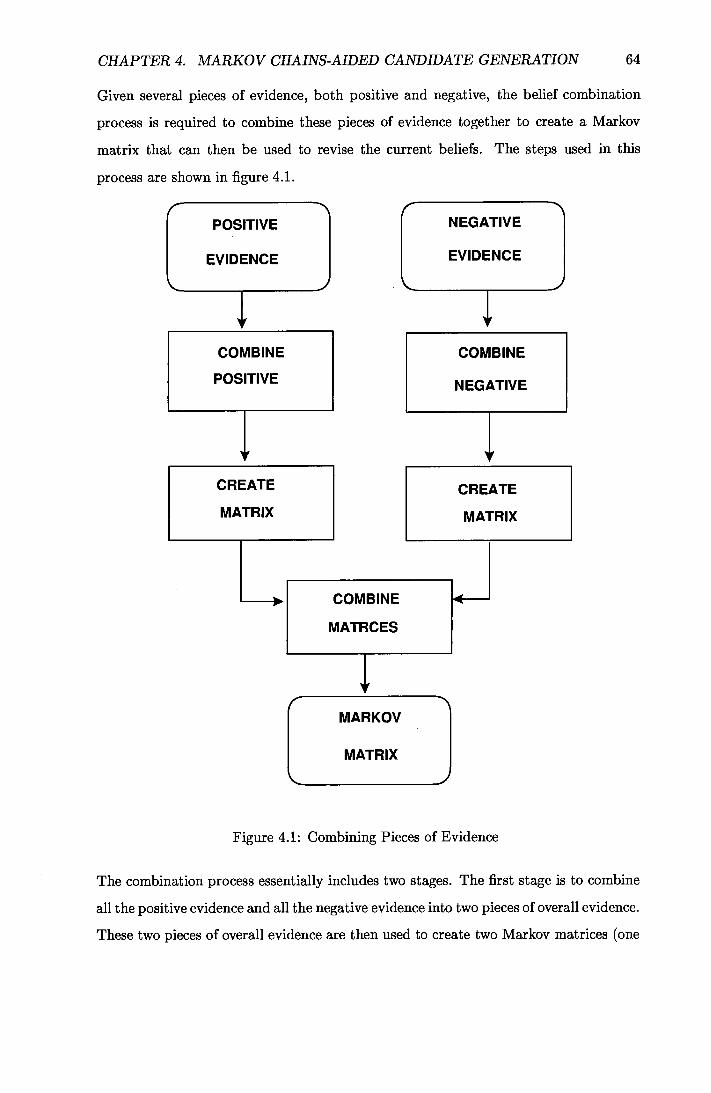
CHAPTER 4. MARKOV CHAINS-AIDED CANDIDATE GENERATION 64
Given several pieces of evidence, both positive and negative, the belief combination
process is required to combine these pieces of evidence together to create a Markov
matrix that can then be used to revise the current beliefs. The steps used in this
process are shown in figure 4.1.
POSITIVE I I NEGATIVE
EVIDENCE I I EVIDENCE
COMBINE I I COMBINE
POSITIVE I I NEGATIVE
CREATE I I CREATE
MATRIX I I MATRIX
COMBINE
MATRCES
MARKOV
L MATRIX
Figure 4.1: Combining Pieces of Evidence
The combination process essentially includes two stages. The first stage is to combine
all the positive evidence and all the negative evidence into two pieces of overall evidence.
These two pieces of overall evidence are then used to create two Markov matrices (one

CHAPTER 4. MARKOV CHAINS-AIDED CANDIDATE GENERATION 65
positive and one negative). The second stage is then to combine these two matrices
into a single one.
In particular, the first step combines the positive evidence into a single value using the
fuzzy DST (as to be described in section 4.3.3) and then uses this value to create a
Markov matrix as described in section 4.1. A similar procedure is carried out for the
negative evidence. The second step combines these two matrices by averaging the two
matrices as described in section 4.5. The result is a single matrix that can then be
used to revise the beliefs in each of the model fragments (in a single component).
This two stage process is required to allow several pieces of positive (or negative)
evidence to reinforce each other. This reflects the increase in the likelihood that a
particular component is faulty as the more conflict sets a component is in, the more
likely it is to be faulty. The second stage allows any components that have both positive
and negative evidence against them have the overall size of the evidence reduced,
reflecting the conflicting evidence. Neither of these two steps would be sufficient on
their own.
If each piece of evidence were used to create a Markov matrix and the resulting matrices
were combined by averaging over all of the matrices, the desired properties would not
be displayed. The resulting matrix would be a Markov matrix, but the effect of the
matrix would not reflect the individual pieces of evidence. For example if two pieces of
positive evidence, of size 0.6 and 0.4 were found for a given component, creating and
then averaging Markov matrices for these two pieces of evidence would create a matrix
as shown below.
A piece of positive evidence of size 0.6 gives the following matrix
1.0 0.6 0.6 0.6 0.6
0 0.4 0 0 0
0 0 0.4 0 0
0 0 0 0.4 0
0 0 0 0 0.4

CHAPTER 4. MARKOV CHAINS-AIDED CANDIDATE GENERATION 66
Similarly, a piece of positive evidence of size 0.4 gives the following matrix:
1.0 0.4 0.4 0.4 0.4
0 0.6 0 0 0
0 0 0.6 0 0
0 0 0 0.6 0
0 0 0 0 0.6
Averaging these two matrices gives the following matrix:
1.0 0.5 0.5 0.5 0.5
0 0.5 0 0 0
0 0 0.5 0 0
0 0 0 0.5 0
0 0 0 0 0.5
The resultant matrix is exactly the same as the matrix that would be obtained if
the two pieces of evidence (0.6 and 0.4) were averaged before generating the matrix
(Theorem 9 shows that this is generally the case). The result of this is that the
resultant matrix reflects an average of the individual pieces of evidence. Several pieces
of positive evidence for a component indicate the component is more likely to be faulty
and so combining two pieces of positive evidence should effectively create a larger
piece of evidence. The averaging of many matrices, therefore, does not allow effective
combination of evidence.
If all of the evidence, both positive and negative, were to be combined together before
creating a Markov matrix a different problem would arise. The DST only works for
positive evidence. The DST could be modified to have two propositions (positive evi-
dence F and negative evidence F), however this would result in two pieces of evidence
(one positive and one negative) which would still need to be combined. The problem
could be avoided by using the method for combining certainty factors (CFs) in MYCIN
[Buchanan & Shortliffe 84], however this method is not associative and so the result of
combining beliefs would depend upon the order of their combination.
Theorem 9 (See Appendix A for proof)
Given 2 pieces of evidence x and y, creating two Markov matrices and then averaging

CHAPTER 4. MARKOV CHAINS-AIDED CANDIDATE GENERATION 67
them gives exactly the same Markov matrix generated by averaging the two pieces of
evidence and then creating a Markov matrix from the result.
4.3.3 Combining Individual Pieces of Evidence
All of the new evidence relating to each of the fragments, both positive and negative,
must be combined to give overall evidence relating to that fragment.
If a model fragment appears in more than one conflict set it is more likely that it
is faulty than if it just appeared in one conflict set. Similarly if a model fragment
appears in more than one confirm set it is less likely that it is faulty then if it had
just appeared in one confirm set. The combination technique must therefore satisfy
the following criteria:
Two pieces of positive evidence must reinforce each other
Two pieces of negative evidence must reinforce each other
The combination mechanism should be associative, so that the order of combi-
nation of the evidence is not important
The proposed method for performing this combination is the Fuzzy DST outlined
below.
Fuzzy DST
DST allows for the maintenance of beliefs to reflect evidence from varying sources.
Fuzzy logic is a means of handling uncertainty in a representation. The aim here is to
combine fuzzy logic and DST to create fuzzy DST which will facilitate the maintenance
of uncertain beliefs.
This combination is required for a specific task, namely the combination of multiple
evidence for or against a particular model fragment. The examples and discussion will
therefore concentrate on a simple example from this domain.

CHAPTER 4. MARKOV CHAINS-AIDED CANDIDATE GENERATION 68
Before describing the fuzzy DST it is necessary to briefly outline the concept of fuzzy
arithmetic.
Fuzzy arithmetic
The fuzzy arithmetic that is to be used is a simplification of the "fuzzy numbers" as
described in [Shen & Leitch 93].
The only differences are that:
only a subset of the basic operations (addition, subtraction and multiplication)
are required as these are the only operations used in the DST.
only positive numbers can exist (numbers in [0, 1]), as the beliefs used can only
take values between zero and one.
triangles will be used instead of trapezoids (triangles are after all a specific in-
stance of the trapezoid), as the exact value of each belief is known.
The triangles are represented as a triple [a, b, c], where a represents the value at the
apex of the triangle, b represents the amount of the triangle to the left and c represents
the amount of the triangle to the right.
There are several reasons for choosing triangles over trapezoids:
Triangles are more intuitive than trapezoids
The calculations are more efficient than for trapezoids
The defuzzification is not only simpler, but also more efficient
Only one "variable" (width) is required for symmetric triangles, compared to the
trapezoids two (width and plateau width) required for symmetric trapezoids
Trapezoids "plateau" increases monotonically, so a large number of calculations
will lead to very wide trapezoids (plateau) which in the limited domain [0, 1] will
become fairly meaningless. The width of the base of the triangle widens after

CHAPTER 4. MARKOV CHAINS-AIDED CANDIDATE GENERATION 69
each arithmetic operation, but then so does the width of the triangular parts of
the trapezoid
The simplified operations thus become (for rn = [a, b, c] and n = [d, e, 1]):
m+ri= [a + d, b + e, c + f ]
m — n = [a — d, b + f , c + e]
m x n = [ad, ae + db — be, af + dc + cf ]
Example
Using the same values as in the DST example in the previous chapter, evidence x = 0.4
and evidence y = 0.6. Fuzzify both pieces of evidence by defining them as fuzzy
numbers centred on their belief with a width of 0.1 (an arbitrary value).
Fuzzy x = [0.4, 0. 1, 0.1]
Fuzzy y = [0.6, 0. 1, 0.1]
Fuzzy DST requires the evaluation of x + y - xy.
In steps (the operators have the same precedence as in normal arithmetic and so the
multiplication is carried out first, whilst the addition and subtraction can be carried
out in any order without affecting the result):
xy = [0.24, 0.09, 0.111
x+y = [1.0, 0. 2, 0.2]
X + y - xy = [0.76,0.31,0.29]

CHAPTER 4. MARKOV CHAINS-AIDED CANDIDATE GENERATION 70
Defuzzification
Having this fuzzy result it is now necessary to convert it into a crisp form. the process
for doing this is called defuzzification.
The simplest defuzzifier is the max value defuzzifier which would simply return the
apex of the triangle (as this is the maximum value in the fuzzy set) which would give
0.76 which is exactly the same as crisp DST (the use of triangles ensures that this is
always the case). Using the centre of gravity defuzzifier gives (0.76 + 0.290.31 ) 0.75,
which is slightly less than crisp DST (again this will always be the same as the triangles
will become skewed to the left, due to the nature of the fuzzy arithmetic).
As using the max value defuzzifier would always give the same value as in crisp DST
(if the triangle is asymmetric this would lead to a loss of knowledge), it is proposed
that the centre of gravity defuzzifier be used. It should be noted that, as the number
of pieces of evidence grows the difference between crisp DST and fuzzy DST will tend
to increase as the triangle becomes more and more skewed.
This approach satisfies all of the required criteria. The fuzzy DST will be used to
calculate two pieces of evidence for each component, one piece of evidence records the
positive evidence and the other records the negative evidence. In general there will be
several pieces of positive evidence and several pieces of negative evidence relating to a
particular model fragment. Using the fuzzy DST all of this evidence can be combined to
create just two pieces of evidence, one positive and one negative. Of course it is possible
that there may be no positive (or negative) evidence, in which case the combination
is not performed. Similarly, if there is only one piece of positive (negative) evidence
there is no need to perform the combination.
In the illustrative example there were four pieces of evidence, two positive and two
negative 0.9, 0.8, -0.2 and -0.3. Fuzzifying these gives [0.9, 0.1, 0.1], [0.8, 0.1, 0.1],
[-0.2, 0.1, 0.1] and [-0.3, 0.1, 0.1].
Combining the two positive values gives [0.98, 0.38, 0.36]. As both these values were
positive the result, as expected, is that the beliefs have reinforced each other giving
a high positive value. Defuzzifying this value gives the overall positive evidence of

CHAPTER 4. MARKOV CHAINS-AIDED CANDIDATE GENERATION 71
0.98+ 0.36-0.38 = 0.97.
Combining the two negative values gives [-0.56, 0.16, 0.14]. As both of these values were
negative the result shows that the negative evidence has been reinforced. Defuzzifying
this value gives final overall negative evidence of —0.56 + 0.140.16 = —0.57.
Generalisation
The techniques illustrated in the above example can be generalised to any values.
Given two pieces of positive evidence x and y, they can be combined into a single piece
of evidence as follows:
Fuzzify the two pieces of evidence to create fuzzy numbers, which are represented
as triangles of width w. This gives the following fuzzy numbers [x, w, w] and
[y,w,w].
Combine these two fuzzy numbers using the expression x + y - xy. The stages
of calculating the fuzzy number are:
xy = [xy, w(x + y - w), w(x + y + w)]
x+y= [x+y,2w,2w]
x+y — xy=[x+y — xy,w(2 +x+y+w),w(2 +x+y — w)]
Defuzzify the result using the centre of gravity defuzzifier. This gives the crisp
result of x + y - xy - w2 .
This process can be repeated for each additional piece of evidence. When combining
multiple pieces of evidence, the fuzzification step could be omitted, though this would
complicate subsequent calculations. By defuzzifying at each step, using a fixed fuzzy
width, the calculations can be considerably simplified, with only the simple calculation
at step 3 being required. If the fuzzification step is not carried out at each step, the
full calculation at step 2 would needed to be performed for every combination.

CHAPTER 4. MARKOV CHAINS-AIDED CANDIDATE GENERATION 72
4.4 Creating the Markov Matrices
Once all of the negative (positive) evidence has been combined into a single piece of
negative (positive) evidence there will, in general, be evidence both for and against
individual fragments. There will be positive and negative evidence for a particular
fragment if that fragment was in both conflict sets and confirm sets. There would be
just positive evidence if the fragment only appeared in confirm sets and only negative
evidence if the fragment only appeared in conflict sets.
In order to use this evidence it is necessary to create Markov matrices for every piece of
evidence. If both positive and negative evidence exists it is necessary to create separate
matrices so that the mixed nature of the evidence is reflected in the belief revision
process. For each of the fragments that were in the model, create a Markov matrix for
each piece of evidence, both positive and negative, where such evidence exists. Each
of these matrices represents an amount of belief, or disbelief, in a particular fragment.
Returning to the example, the two pieces of overall evidence are 0.97 and -0.57 so a
matrix is created for each piece. The overall positive evidence (0.97) gives the following
matrix:
1.0 0.97 0.97 0.97 0.97
0 1-0.97 0 0 0
0 0 1-0.97 0 0
0 0 0 1-0.97 0
0 0 0 0 1-0.97
which simplifies to:
1.0 0.97 0.97 0.97 0.97
0 0.03 0 0 0
0 0 0.03 0 0
0 0 0 0.03 0
0 0 0 0 0.03
The overall negative evidence (-0.57) gives the following matrix:

CHAPTER 4. MARKOV CHAINS-AIDED CANDIDATE GENERATION 73
1 1.0+ (-0.57) 0 0 0 0 1 -(-0.57 x---) 1.0 0 0 0
Cl I
I -(-0.57 x-u--) 0 1.0 0 0 I 1-cr I
(0.57 X 0 0 1.0 0Cl I
L -(-0.57 x- a--) 0 0 0 1.0] 1-ci
where ci, C2, C3, C4 and C5 are the current beliefs in each of the fragments (0.8, 0.09,
0.06, 0.04 and 0.01 respectively).
Substituting these values into the matrix gives:
1.0 + (-0.57) 0 0 0 0
-(-0.57 x 1.0 0 0 0
-(-0.57 x i ) 0 1.0 0 0
-(-0.57 xi -%0- 4 ) 0 0 1.0 0
-(-0.57 X 1 0-01 0 0 0 1.0
Simplifying this matrix gives:
0.43 0 0 0 0
0.2565 1.0 0 0 0
0.171 0 1.0 0 0
0.114 0 0 1.0 0
0.0285 0 0 0 1.0
The result is two matrices that represent the positive and negative evidence relating
to the fragment fl. If the positive matrix were applied to the current beliefs, the
belief in fragment fi would be considerably increased, with a corresponding decrease
in the beliefs of each of the other fragments of that component. Similarly, if the
negative matrix were applied to the current beliefs, the belief in fragment f' would be
considerably reduced, with a corresponding increase in each of the other beliefs. Given
the final evidence, these two matrices were easily derived. As the positive matrix and
the negative matrix are fairly sparse, the number of matrix elements that needed to
be calculated is small. If the number of model fragments were doubled the number of

CHAPTER 4. MARKOV CHAINS-AIDED CANDIDATE GENERATION 74
extra calculations would also double and so the complexity of the matrices is linear
with respect to the number of model fragments, which is very important in controlling
the overall complexity of the process.
4.5 Combining the Markov Matrices
The penultimate step in the process is the combination of all the individual matrices
into a single matrix. This is necessary to ensure that the belief revision process is
consistent. If the matrices were applied to the current beliefs separately, the ordering
of their application would have a significant impact on the revised beliefs. If the
two matrices were combined and the resultant matrix applied to the current beliefs,
the results would be consistent. An additional advantage of this approach is that
matrix multiplication is a relatively expensive operation, and so only performing it
once improves the overall efficiency.
The combination must still reflect each of the individual updates suggested by each
of the individual matrices, as well as still maintaining the properties of a Markov
matrix (the values in each column should sum to one). It is important that each
of the individual updates is reflected in the final combined matrix, otherwise data
or information that was available to the system will have been wasted. From a more
practical point of view reflecting each of the individual updates ensures that, in general,
the certainties associated with different components will be updated in different ways
making the selection of different models at the next step more likely. It is important
that the properties of a Markov matrix are maintained as this ensures that the sum
of the updated certainties will still be one, which is essential as one of the fragments
must represent the actual behaviour of the component.
The proposed method is to average the individual elements of each matrix to give a
single matrix. This method was chosen, because it is very simple and the result still
reflects both of the original matrices, so that the relative size of both the positive and
the negative evidence will still have an influence on the belief revision. For example, if
the following two matrices were to be combined:

CHAPTER 4. MARKOV CHAINS-AIDED CANDIDATE GENERATION 75
1 i i i
1—i 0 0
o 1—i 0
o 0 1—i
and
1—j 0 0 0
1—j 0 0
o 1—j 0
j j j 1
the result would be:
1+1-j k I
1-i1-j
0 0 1i+1j
1-j+1 2 2 2 2
which equals
2 2 2 2 i_:I 0 0
o o 1_2 0
.i 1- 2 2 2 2
These matrices satisfy the criteria of combination. In particular each column still sums
to 1.
Another possible method of combining Markov matrices would be to multiply each
of the matrices together. The product would still be a Markov matrix [Stewart 94].
However this method is not satisfactory as not only is there no underlying meaning to
this combination, but the order of combination will affect the final result. The proposed
method, on the other hand, represents both values and the order of combination is
unimportant.

CHAPTER 4. MARKOV CHAINS-AIDED CANDIDATE GENERATION 76
Theorem 10 (See Appendix A for proof)
If A,,-, An are Markov matrices, then averaging across individual elements results in
a Markov matrix.
Applying this averaging approach to the two matrices in the example gives:
r 1.0+0.43 0.97+0 0.97+0 0.97+0 0.97+0 1 I 2 2 2 2 2 I I 0+0.2565 0.03+1 0 0 0 I I 2 2 I
I 0+0.171 0 0.03+1 0 0 I I 2 2 I
0+0.114 [ 0 0 0.03+1 0 I 2 2
0+0.0285 0 0 0 0.03+1 I 2 2 .J
Simplifying this matrix gives:
0.715 0.485 0.485 0.485 0.485
0.12825 0.515 0 0 0
0.0855 0 0.515 0 0
0.057 0 0 0.515 0
0.01425 0 0 0 0.515
This matrix reflects both aspects of the evidence. Despite the overwhelmingly strong
positive evidence the negative evidence has a major impact on the final matrix. This
reduction in the effect of the positive evidence is acceptable as the initially high positive
evidence has to be tempered by the moderately high negative evidence against the
model fragment.
Revise the Certainties
The final step is updating the certainties. If the matrix derived as per the technique
described in the previous section is M and the current certainties are given by the
column matrix C then the revised certainties Cnew are calculated as:
Cnew = MC

CHAPTER 4. MARXOV CHAINS-AIDED CANDIDATE GENERATION 77
The elements of now represent the belief in each of the model fragments after
the evidence generated by the current model has been applied, as they reflect both the
previous beliefs and the evidence that was generated during the previous simulation.
Continuing with the simple illustrative example, the matrix M is the one derived above
and the transposed vector CT is [0.8, 0.09, 0.06, 0.04, 0.01]. The values of are
therefore [0.669, 0.14895, 0.0993, 0.0662, 0.01655].
The belief in fragment fi has been reduced slightly despite the strong positive evidence
in favour of it, this is due to the negative evidence which casts some doubt over the
correctness of the fragment. The beliefs in each of the other fragments has increased
slightly to reflect this. It is important to note that the relative beliefs in fragments
f2, 13, f 4 and f 5 is unchanged with respect to each other as there was no evidence to
distinguish between them.
This chapter developed the use of Markov Chains for candidate generation. Evidence
for and against individual model fragments is used to revise the beliefs. The result is
a process that uses all of the available evidence in suggesting fault candidates. The
ideas were developed both as a general belief revision process and, in particular, as a
process for candidate generation in static physical systems.

Chapter 5
Comparison with Existing Static
Techniques
To illustrate the effectiveness of the techniques described in the previous chapter
[Smith & Shen 99, Smith & Shen 00] a simple example problem will be considered.
A more comprehensive example will be presented in the next chapter. The prob-
lem will be the same as that used in chapter 2 when describing the GDE algorithm
[deKleer & Williams 87]. The GDE algorithm is not considered here, partly because
the example has already worked through but mainly because GDE only considers a
component to be faulty or not faulty. The comparison here will be between systems
that incorporate fault models and will highlight the differences between the approaches
and discuss the relative computational complexity of each of them.
All of the approaches compared in this section use the same underlying technique for
detecting faults (the GDE inference engine), indeed many model-based static diagnos-
tic systems share the same core as do some recent approaches to dynamic diagnosis
[Dvorak & Kuipers 91, Struss 97]. The discussion of the complexity of each of the tech-
niques will therefore focus on the processes for belief revision. There are two potential
sources of increased complexity when scaling this problem to a more realistic one:
. An increase in the number of components. This is the most obvious increase in
complexity, as the number of components increases so does the complexity of the
belief revision process.

CHAPTER 5. COMPARISON WITH EXISTING STATIC TECHNIQUES 79
An increase in the average number of possible behaviours for each of the compo-
nents. This increase in complexity can lead to a temptation to reduce the number
of behaviours used for each component, but this can have a detrimental effect on
the diagnostic process as the potential for correctly identifying faults is reduced.
It is therefore desirable that an increase in the number of possible behaviours
does not have too great an effect on the complexity of the problem. The average
number of possible faults, certainly for simple components such as adders and
multipliers, is unlikely to be very large. The effect of complexity on the number
of possible behaviours is therefore less important than for the number of compo-
nents. The relative importance of the number of components is reinforced by the
fact that the number of components will generally be significantly greater than
the average number of behaviours. A physical system may have several thousand
components and yet less than 10 behaviours per component.
5.1 The System under Diagnosis
The simple example used here is not overly complex, however the effects of scaling the
problem up to a more realistic size are also addressed. For convenience the diagram
illustrating the problem is repeated in figure 5.1.
5.2 Markov Chains for Belief Revision
The first technique that will be considered is the work proposed in this thesis, the
use of Markov Chains for belief revision. Suppose that each of the components in the
system are modelled by seven different model fragments and, for simplicity, that all of
the components have the same set of model fragments. In particular, each component
has a model fragment that corresponds to the desired "normal" behaviour (F1), five
known fault behaviours (F2 to F6) and an unknown fault behaviour (F7). Each of the
model fragments can be identified by its name which is of the form CFi that represents
model fragment F(i = 1, 2,..., 7) of component C(C E {M1, M2, M3, Al, A2}). The
initial values of the beliefs were set to 0.99 for each OK fragment, 0.00001 for each

CHAPTER 5. COMPARISON WITH EXISTING STATIC TECHNIQUES 80
A -2
=2
1
Figure 5.1: Illustrative Diagnostic Problem
unknown fragment and 0.001998 for all of the other fragments. These value for the OK
fragments is reasonable as in general most components will not fail and so the belief in
each of them should be relatively high. Similarly, the belief in the unknown fragment
is low as it is relatively unlikely to fail in an unknown manner. In the absence of
any detailed fault frequencies, the known fault models are all assigned the same initial
belief.
When the diagnostic process is invoked, there are no known conflict sets yet and the
most believed system model is the "normal" behaviour model. This model is selected
and analysed using GDE's conflict recogniser. The following minimal conflict sets
were generated: {M1F1 Alp1 M2F1 }, {M1F1 M3F1 A2 1 A11 }, {M2F1 M3F1 A21 },
resulting in pieces of penalising evidence. For example, fragment {M2p1 } appeared in
two conflict sets and so generated two pieces of evidence which need to be combined
into a single piece of evidence E1. The values of the two pieces of evidence were -
and - (since all the fragments have the same current belief) which gives E1 = -
Table 5.1 shows all of the evidence generated by this system model.
There are no confirming sets detected and so there is no rewarding evidence. The

CHAPTER 5. COMPARISON WITH EXISTING STATIC TECHNIQUES 81
Table 5.1: The Evidence Generated
Model
Fragment Evidence Evidence
Combined
Evidence
.PVI1F 1 1 - 1 - 1 -
M2F1 1 - 1 - _5
M3F1 1 - 1 - 1 -
A1F1 1 - 1 - 1 -
A2F1 1 - 1 - 1 -
values of the beliefs are then revised, using the penalising evidence against each of the
fragments in the system model. Table 5.2 shows the revised values of belief in each of
the fragments (rounded to three decimal places). From these revised beliefs and the
known conflicts, the most likely model, that contains no known conflicts is selected and
the process iterates. In this case the selected model contains the following fragments:
M1F1 , M2F2, M3F1 , A1F2 and A2F1 .
Table 5.2: The Revised Beliefs
Fragment
Name Ml M2 M3 Al A2
F1 0.495 0.44 0.495 0.495 0.495
F2 0.1 0.111 0.1 0.1 0.1
F3 0.1 0.111 0.1 0.1 0.1
F4 0.1 0.111 0.1 0.1 0.1
F5 0.1 0.111 0.1 0.1 0.1
F6 0.1 0.111 0.1 0.1 0.1
F7 0.0005 0.0006 0.0005 0.0005 0.0005
After seven iterations (i.e. having chosen seven system models) a fault hypothesis is
found with M1F2 and M2F5 being the faulty components, which correctly explains the
observed behaviour. The fragment M2F5 was the 5th model fragment that had been
considered for component M2, and so most of the system models that were considered
were there to evaluate the various possibilities for component M2. If model fragment
M2p5 had represented the most likely fault behaviour for component M2, then the

CHAPTER 5. COMPARISON WITH EXISTING STATIC TECHNIQUES 82
fault would have been identified after only 3 iterations, as the most likely fragment
would have been considered first.
Each of the components has its belief revised independently of the others, though the
values of the beliefs are dependant on the behaviour of the other components in the
model. Additionally the cost of revising the belief for a component is fixed (assuming
that the number of possible behaviours stays constant). Therefore the effect of doubling
the number of components is to double the effort involved in revising the beliefs. The
complexity of the belief revision process is therefore linear with respect to the number
of components in the model, thereby being readily scaleable with respect to the number
of components. The complexity of the model selection process is non-linear, as it almost
performs a brute-force search.
The complexity of the conflict recognition process is also non-linear as the number and
size of the conflict sets generally increase with respect to the number of components
in the model. The significance of this complexity is reduced as the same conflict
recognition process is also utilised in both GDE+ and Sherlock.
The average number of possible behaviours on the other hand has potentially a greater
complexity. The generation of the Markov matrices used is itself linear as the matrices
are sparse, because generally all but two elements in each of the columns are zero. The
complexity increases for the application of the matrices as the process is effectively a
matrix multiplication and so rather than being linear the complexity is 0(n2) (where
ii is the number of possible behaviours). This is not a serious problem as long as the
average number of behaviours is relatively small, which is a reasonable assumption
as argued previously. This problem is further reduced as the matrices themselves are
sparse which greatly increases the efficiency of the multiplication.
5.3 GDE+
An existing system that utilises a similar set of possible fault behaviours is GDE+
[Struss & Dressler 89]. GDE+ [Struss & Dressler 89] starts in the same way as in the
previous example and generates the same minimal conflict sets. The process then
determines the minimal fault candidates (as in GDE) and generates the following

CHAPTER 5. COMPARISON WITH EXISTING STATIC TECHNIQUES 83
minimal sets
{M1, M21 {M1, M31 {M1, A21 {A1, M21 {A1, M31 {A1, A21 {M2, M3} {M2, A2}
GDE+ now tries to evaluate possible faults from all the possible fault behaviours. If
it is assumed that all of the possible behaviours are as given in the previous example
there are 5 possible faults for each component (if the unknown behaviour is ignored as
GDE+ simply cannot handle this). There are therefore 25 possible fault combinations
for each of the minimal candidate sets. As there are 8 minimal candidate sets a total of
200 fault combinations need to be considered (assuming that only two components are
actually faulty). As all possible fault behaviours are required by GDE+ the values will
in general be considerably greater than these. GDE+ is therefore particularly affected
by an increase in the average number of possible behaviours.
When GDE+ is applied to larger, more practical, diagnostic problems the complexity
greatly increases. As the number of components increases, so generally does the size of
the conflict sets, this is because the predicted values tend to be derived through more
components. Additionally, if the system under diagnosis has more inputs and outputs,
the number of conflict sets also increases. Whilst the computational complexity of
GDE+ is not directly dependant on the number of components in the system under
diagnosis, this increase in the size (and possibly number) of conflict sets has a significant
effect. As the size or number of conflict sets increases, the number minimal fault
candidates increases and therefore of fault combinations that GDE+ needs to consider
also increases.
The relative number of fault combinations that needs to be considered depends upon
the number of faulty components in the system under diagnosis. If there is only
a single fault, the number of fault combinations only increases linearly (assuming a
fixed number of possible fault behaviours). This is because each additional member
of a conflict set only requires a fixed increase (the number of possible faults) in the
number of fault combinations. However, when two or more faulty components are
present the complexity increases exponentially. In this case, as every fault behaviour
needs to be considered in combination with every fault behaviour of all of the other
suspected components. The problem is considerably worse when more than two faulty
components are present. As an example, consider a system where each component has

CHAPTER 5. COMPARISON WITH EXISTING STATIC TECHNIQUES 84
five possible behaviours. If a single faulty component exists, five fault combinations will
need to be considered for each member of the conflict sets, therefore each additional
member of a conflict set increases the number of fault combinations by five. If two
faults occur, each conflict set generates 25 (5 x 5) fault combinations. If only two
components are suspected, the total number of fault combinations is just 25, however
if three components are suspected, the total number of fault combinations is 75 (25 for
each possible combination). When four components are suspected the total number
of fault combinations is 300 (again 25 for each possible combination), the increase in
computational complexity is therefore non-linear.
5.4 Sherlock
Another system that uses an identical type of possible model (including the unknown
fault model) is Sherlock [deKleer & Williams 89]. Sherlock starts in the same way as
GDE+. The minimal conflict sets are used to focus the search for possible diagnoses.
In order to generate leading candidates it then uses approximate prior probabilities in
the same form as the Markov Chain process. It only considers the most likely faults
initially, and only considers the less likely faults if the most likely ones have been
eliminated. The problem with this approach is that in order to find leading candidates
a considerable number of potential candidates may have to be considered.
The above problem is compounded if the size and number of the conflict sets increases,
as this significantly increases the number of possible models that need to be considered.
The process is roughly linear with respect to the number of components primarily due
to the focusing mechanism. The complexity is more dependant on the size and number
of the conflict sets, as either of these increases so generally does the size of the focus
of the diagnosis, which subsequently increases the complexity. The effect is similar to
that observed in GDE+, except that as Sherlock searches for the most likely faults, the
complexity with respect to the average number of behaviours is partially dependant on
the relative probabilities of each of the behaviours. However, as Sherlock may consider
candidates whose probability is th of the best candidate an increase in the number 100
of behaviours can have a considerable detrimental effect on the candidate selection

CHAPTER 5. COMPARISON WITH EXISTING STATIC TECHNIQUES 85
process.
5.5 Summary
The process that uses Markov Chains for belief revision has complexity advantages over
both GDE+ and Sherlock, both in terms of the number of components and the average
number of behaviours. In particular it uses information from each model simulation
to guide successive candidate selection processes. In addition, as it only considers one
candidate at a time the potential for complexity problems is considerably reduced.

Chapter 6
Experimental Evaluation of the
Approach
The previous chapter compared the techniques in this thesis with other approaches
using a simple example. This chapter presents the results of systematically using the
techniques described in the thesis on a non-trivial system. Multiple faults will be
simulated in the system under diagnosis and then the performance of the diagnostic
process will be evaluated by its ability to identify the simulated fault in as few attempts
as possible.
6.1 The System under Diagnosis
The system used to obtain these results is described below, with Appendix B detailing
its components.
The physical system is built from two types of components, adders and multipliers.
An adder has two inputs and one output, with the output being the sum of the two
inputs. A multiplier also has two inputs and one output, with the output being the
product of the two inputs.
The system under diagnosis is built from full adder [deKleer & Williams 87] mod-
ules as shown in figure 6.1. These modules consist of 5 individual components (3
multipliers and 2 adders) and have five inputs and two outputs. These modules are
M.

CHAPTER 6. EXPERIMENTAL EVALUATION OF THE APPROACH 87
IN1
1N2
1N3
1N4
1N5
OUT1
OLJT2
Figure 6.1: Low Level Detail of the System Under Diagnosis
used to build the full system as shown in figures 6.2 and 6.3. There are fifty inputs
(A1..A10, B1..B10, C1..C10, D1..D10 and E1..E10) AND 16 outputs (ol..o16) in
the system overall. In figures 6.2 and 6.3 the elements labelled 1 - 18 each represent
an instance of the module shown in figure 6.1. Figure 6.2 shows how the inputs are
used to derive values for the system variables F1..F10 and GL .G10. Note that the
values of these system variables are not measurable. The components in figure 6.3 take
these system variables and derives the system outputs. The system has a total of 90
components (54 multipliers and 36 adders) and each of the inputs has an effect on up
to eight of the outputs. The system is therefore reasonably complex and provides a
test bed for evaluating the techniques described in this thesis.
6.1.1 Behavioural Fragments for Each Component
For each of the components in the system model 4 possible model fragments were
defined, each of which, in conjunction with the fragment models of other system com-
ponents, could explain the behaviour of the system.
The details of each of these behaviours is as follows:
1. Normal behaviour. The component behaves as it is expected to, representing the
component not being faulty. The prior certainties, p(no'rmal), were set to 0.99
to reflect the low probability that any individual component is faulty.
2. Stuck at zero (denoted by sO). This fragment returns the value zero, no matter

CHAPTER 6. EXPERIMENTAL EVALUATION OF THE APPROACH 88
Al
B1 F1
cl
D1 G1 El
__________________ F2
D2 G2
B3 F3
D3 G3
A4
B4 :E~E F4
C4 4 D4 4 E4
F5
D5 G5
F6 B6
D6 G6
FF
F7
D7 G7
AB
B6 F8
08 G8
AS F9
B9
D9 G9
AlE B10 lo F10
clo
E10 Gb
Figure 6.2: Level 1 of the System Under Diagnosis

CHAPTER 6. EXPERIMENTAL EVALUATION OF THE APPROACH 89
01
G2 o2
o3
G4 12 o4
F7 Ec 13 G7 06
G8 07
F10 :Ec 14 _08
Gb
F1 09 ___________________
oiO
oil
F8
EEff 16 F9 o12
G3
EE4: 17
o13
G4 o14
GG o15
G7 18 016
Gb 0
Figure 6.3: Level 2 of the System Under Diagnosis

CHAPTER 6. EXPERIMENTAL EVALUATION OF THE APPROACH 90
what the value of the inputs. This behaviour fragment has the effect of altering
the theoretical structure of the model as the flow from inputs through to outputs
has been altered. This feature highlights the possibility of allowing the structure
of the model to change as well as the behaviour of individual components. It
can be easily seen that a simple extension to the current model, through the use
of different model fragments would easily allow the structure of the model to be
changed. This could be achieved by allowing various model fragments, for the
same component, to have different inputs and outputs. As it is the relationship
between the inputs and outputs of the various components that effectively defines
the structure of the model, allowing them to vary effectively allows the model
structure itself to vary. The prior certainties, p(sO), were set to 0.0049999 as it
was assumed that known faults were more likely than unknown faults.
Stuck at one (denoted by si). As with the previous fragment, this behaviour
effectively changes the structure of the model. This time however, the output is
1 no matter what the inputs are. The prior certainties, p(sl), were set to the
same value as p(sO), 0.0049999.
Unknown (denoted by u). This fragment represents the case where the fault is
unknown. Again this fragment effectively changes the structure of the model, as
it alters the flow of information through the model as it has no inputs or outputs.
Note that the diagnostic engine cannot propagate through a component whose
behaviour is unknown. It is very useful to have such behaviours available, despite
having no knowledge of their behaviour as they allow the diagnostic system to
diagnose a fault in a component without necessarily knowing exactly how that
component has failed. The prior certainties, p(u), were set to 0.0000002 as it was
assumed that an unknown fault was unlikely.
The model used has 90 components of various types, each of which has 4 possible
behaviours. The total number of possible models is therefore:
490 1 x 1054
Clearly it would be impossible to try all possible models and find possible faults ex-

CHAPTER 6. EXPERIMENTAL EVALUATION OF THE APPROACH 91
haustively.
6.2 Experimental Methodology
To evaluate the diagnostic method described in this thesis it is necessary to perform
a significant number of diagnoses. A total of 100 multiple faults were simulated and
attempts were made to diagnose the faults.
Each of the attempts at diagnosis was generated randomly. In each case two faults were
simulated by randomly selecting two of the components and then randomly allocating
them one of the two known faults (sO or si). The inputs for each test were also
generated randomly to avoid any bias introduced by a single set of inputs being used
in each test. Each test ran until the actual fault was found, if other fault candidates
were proposed before the actual fault the test continued.
To evaluate the performance of each test two factors were measured:
The number of models simulated before the correct faults were found. This
measurement is important as the aim of the diagnostic process is to find the
actual fault as quickly as possible.
The second method for evaluating each model is to consider the prior certainty of
each of the models that were simulated. It is important that the models should
be considered in order of prior certainty, otherwise less likely candidates may be
suggested before more likely ones.
6.3 Results
The results of the one hundred tests are presented in this section. The tables that show
the results of individual tests only indicate those components that are not behaving
in their non fault mode. The empty portions in some of these tables are for models
that contain fewer faulty components than in some of the other simulations in that
particular test.

CHAPTER 6. EXPERIMENTAL EVALUATION OF THE APPROACH 92
6.3.1 The Number of Models Simulated
The number of models simulated for each test are shown in table 6.1. The average
number of models simulated in these one hundred tests was 4.62, indicating that the
process is very efficient at identifying faults in this physical system. In eleven cases the
correct fault was identified in the first model to be simulated. There were thirteen tests
that took ten or more models, with the largest number of models (seventeen) being
simulated in the final test. This compares very favourably against the total number of
models that may have to be simulated in exhaustive search.
Figure 6.4 shows the distribution of the number of models simulated. This clearly
shows that the majority of the faults are correctly identified within four models, and
only a few tests taking more than eleven models to correctly identify the faults.
The tests that took four or less model simulations were generally tests where the faults
did not interact with each other. These cases were effectively two single faults and the
search for fault candidates was a search for two distinct faults which quickly focuses
on a small set of components. An example of a test where the correct faults were
detected very quickly is test 8, the details of which are shown in table 6.2. In this
case, one of the faulty behaviours is correctly identified in the first model simulated
(component add13 displaying fault sO), the subsequent models are then used to search
for the second fault.
The tests where the faults did not interact with each other are indicated in table 6.1
by not having a '' in the Models column. These results are summarised in figure
6.5, which shows that most of this kind of fault were correctly identified within four
models. All of the faults were correctly identified within nine models. The average
number of model simulations in these tests was 3.27. The generally low number of
models considered in these tests confirm that such tests are simpler to diagnose.
The tests that took more than ten model simulations were generally tests where the
faults did interact with each other. In these cases the search for fault candidates is
more difficult as a model that contains only one of the faults does not reduce the
number of conflict sets. The result that when one of the actual faults appears in a
candidate model, it may not be in all subsequent models (unlike the example shown

CHAPTER 6. EXPERIMENTAL EVALUATION OF THE APPROACH 93
Table 6.1: The Number of Models Simulated for each Test
Test Models Test Models Test Models Test Models Test Models
1 3 21 4 41 1* 61 3 81 1*
2 3 22 3 42 4 62 4 82 9*
3 2* 23 4 43 4* 63 2 83 7
4 7* 24 2* 44 9* 64 3 84 4
5 11* 25 2 45 1* 65 11* 85 1
6 6* 26 8 46 3 66 10* 86 1
7 2 27 4 47 2 67 2 87 10*
8 4 28 13* 48 9 68 1 88 2
9 3* 29 4 49 6 69 6 89 4*
10 15* 30 2* 50 5 70 7* 90 2
11 3 31 1 51 2 71 2 91 2*
12 7 32 7* 52 2 72 3 92 4
13 10* 33 3 53 2 73 11* 93 1
14 4* 34 5 54 11* 74 1 94 12*
15 4 35 11* 55 4 75 5 95 2
16 1 36 4 56 2 76 14* 96 4
17 2 37 6 57 1 77 2 97 4
18 7* 38 3* 58 4 78 3 98 4*
19 3 39 4 59 1* 79 2 99 2
20 3* 40 2 60 8* 80 4 100 17*
above). An example of a test which needs more than ten model simulations is test 5
the details of which are shown in table 6.3. In this example one of the actual faults
(component mult3l displaying fault sl) is found after only four simulations, with the
remaining simulations trying to find the other fault.
The tests where the faults did interact with each other are indicated in table 6.1
by having a '' in the Models column. These results are summarised in figure 6.6,
which shows that most of this kind of fault were correctly identified within eleven
models. All of the faults were correctly identified within seventeen models. The average
number of model simulations in these tests was 7.03. These tests generally require

CHAPTER 6. EXPERIMENTAL EVALUATION OF THE APPROACH 94
1I simulated
20
15
We
5
0 0 2 4 6 8 10 12 14 16 18
Number of models simulated
Figure 6.4: Summarised results
more model simulations than those where the faults do not interact, which confirms
the expected increase in complexity in diagnosing such faults. Despite the generally
poorer performance of tests where the faults did interact, only considering an average
of approximately seven models is impressive when compared to the number of possible
models.
6.3.2 Single Fault Solutions
Several tests generated candidates with only single faults, despite two faults actually
being present. In each of theses cases, the single fault was one of the actual faults that
had been simulated. There are two reasons why single faults can be suggested when
two faults are known to exist:
A faulty component is not giving an erroneous output. If this occurs the compo-
nent is not observed to be faulty. For example, if a multiplier is displaying the

CHAPTER 6. EXPERIMENTAL EVALUATION OF THE APPROACH 95
18
16
14
12
' 10 C w a- a
LL 8
6
4
2
I I I U 'Modek simulated
I I I I I I I I
0 2 4 6 8 10 12 14 16 18
Number of models simulated
Figure 6.5: Summarised results where the faults do not interact
faulty behaviour sO and has inputs 3 and 0 then the expected output is 0. In
this case the expected output is produced, despite the component being faulty.
The two faults directly interact with each other. In this case only one of the
components will appear to be faulty. For example, if components multi and
addl were both displaying the faulty behaviour sl, only the fault in component
addl would be detected. The reason for this is that the output from component
multi is only used as an input by component addl and so with both components
being faulty the fault in component multi cannot be detected.
As the diagnostic process only finds minimal fault candidates it cannot suggest the
actual faults as a fault candidate in such cases, though it will identify one of the
components as being faulty on its own.

5
4
CHAPTER 6. EXPERIMENTAL EVALUATION OF THE APPROACH 96
Models simulated"
PH 1fl 0 2 4 6 8 10 12 14 16 18
Number of models simulated
Figure 6.6: Summarised results where the faults do interact
6.3.3 The Prior Certainties of Simulated Models
In most of the one hundred tests performed the models were simulated in order of
decreasing prior certainty. In only two tests were models of a lower prior certainty
considered before models of a higher prior certainty, namely test 37 and test 100. The
results of these two tests are shown in tables 6.4 and 6.5.
In test 37 one of the actual faults was found in the first simulated model and was in all
of the subsequent models. The other faulty component was considered in the second
simulated model, though with the wrong model fragment, despite this the correct
fragment was not considered for another 4 models.
In test 100 eight single faults were tested (though they did not explain the observed
behaviour) including one of the actual faults. This test was the one that considered
the most models of all of the tests performed. What has happened in this test is that
the beliefs have been revised to the extent that models with lower prior certainty are

CHAPTER 6. EXPERIMENTAL EVALUATION OF THE APPROACH 97
Table 6.2: The Results of Test 8
Model Faulty Faulty Prior Still
Number Component Behaviour Component Behaviour Certainty Conflicts?
1 add 13 so add 33 so 1.03E-05 YES
2 add 13 so mult 49 so 1.03E-05 YES
3 add 13 so add 33 si 1.03E-05 YES
4 add 13 so mult 49 si 1.03E-05 NO
considered before those with higher prior certainty.
6.4 Discussion
The results presented in this chapter are generally very encouraging, the results are
found, on average, in less than five models. The diagnostic process very quickly focuses
the search for faults on a few components, with the slowest test taking 17 models to
correctly identify the actual faults.
In 98% of the tests the models were simulated in decreasing order of prior certainty.
In the other 2% of tests this ordering did not occur. The reason that these two tests
did not follow the ordering was that the beliefs had been revised to the extent that
the beliefs in some of fault behaviours rose above that of non-fault behaviours and
so models with three faults were considered before those with only two faults. The
prior certainty in the normal behaviour fragment in each component was set to 0.99,
combining the certainties for the normal behaviour model give an overall prior certainty
of 0.405. This suggests that 60% of the time at least one of the components will be
faulty. If the prior certainty in each of the normal behaviour fragments were increased
to 0.9999 the overall prior certainty becomes 0.99, suggesting only a 1% chance of faults
occurring.
The two tests that did not follow the decreasing prior certainty order were repeated
with the prior certainty in the normal behaviour fragments increased to 0.9999 (the

CHAPTER 6. EXPERIMENTAL EVALUATION OF THE APPROACH 98
Table 6.3: The Results of Test 5
Model
Number
Faulty
Component Behaviour
Faulty
Component Behaviour
Prior
Certainty
Still
Conflicts?
1 add 1 so add 10 so 1.03E-05 YES
2 add 21 so add 24 so 1.03E-05 YES
3 add 21 sl add 24 sl 1.03E-05 YES
4 mult 31 so mult 36 so 1.03E-05 YES
5 mult Si sl mult 36 sl 1.03E-05 YES
6 add 10 sl mult 31 sl 1.03E-05 YES
7 mult Si sl mult 35 so 1.03E-05 YES
8 mult 14 so mult 31 sl 1.03E-05 YES
9 mult 15 so mult 31 sl 1.03E-05 YES
10 mult 31 sl mult 35 sl 1.03E-05 YES
11 mult 15 sl mult Si sl 1.03E-05 NO
Table 6.4: The Results of Test 37
Model
Number
Faulty
Component Behaviour
Faulty
Component Behaviour
Faulty
Component Behaviour
Prior
Certainty
Still
Conflicts?
add IS so add 24 so 103E-05 YES
2 mult 19 so add 24 so 1.03E-05 YES
3 add IS sl add 24 so 1.03E-05 YES
4 add 15 so add 24 so mutt 58 so 5.21E-08 YES
5 add 24 so mult 58 sl mutt 47 so 5.21E-08 YES
6 mult 19 sl add 24 so 1.03E-05 NO
other prior certainties were revised accordingly). The results of these two additional
tests are shown in figures 6.6 and 6.7. The problem of not selecting models in decreasing
order of prior certainty has been resolved for both of these cases.
The results presented here suggest that caution is required when setting the prior
certainties to prevent less certain models being considered before more certain ones.
However, if prior certainties which are closer to the prior probabilities of individual
components failing are used the models should only be considered in decreasing order
of prior certainty.

CHAPTER 6. EXPERIMENTAL EVALUATION OF THE APPROACH 99
Table 6.5: The Results of Test 100
Model
Number
Faulty
Component Behaviour
Faulty
Component Behaviour
Faulty
Component Behaviour
Prior
Certainty
Still
Conflicts?
1 add 1 so 0.002044 YES
2 add 1 51 0.002044 YES
3 malt 1 so 0.002044 YES
4 malt 1 91 0.002044 YES
5 add 3 so 0.002044 YES
6 malt 2 so 0.002044 YES
7 add 21 so add 29 so 1.03E-05 YES
8 add 21 sl add 29 sl 1.03E-05 YES
9 malt 31 so malt 43 so 1.03E-05 YES
10 malt 31 sl malt 43 51 1.03E-05 YES
11 malt 5 so 0.002044 YES
12 malt 32 so malt 43 sl 1.03E-05 YES
13 malt 4 so malt 43 sl 1.03E-05 YES
14 malt 4 sl malt 43 51 1.03E-05 YES
15 add 3 sl 0.002044 YES
16 malt 31 sl malt 32 sl malt 43 sl 5.21E-08 YES
17 malt I SO malt 43 sl 1.03E-05 NO
Table 6.6: The Results of the Revised Test 37
Model Faulty Faulty Prior Still
Number Component Behaviour Component Behaviour Certainty Conflicts?
1 add 13 so add 24 so 1.03E-05 YES
2 mult 19 so add 24 so 1.03E-05 YES
3 add 13 sl add 24 so 1.03E-.05 YES
4 mult 19 sl add 24 so 1.03E-05 NO

CHAPTER 6. EXPERIMENTAL EVALUATION OF THE APPROACH 100
Table 6.7: The Results of the Revised Test 100
Model
Number
Faulty
Component Behaviour
Faulty
Component Behaviour
Prior
Certainty
Still
Conflicts?
1 add 1 so 4.96E-05 YES
2 add 1 si 4.96E-05 YES
3 mult 1 so 4.96E-05 YES
4 mult 1 si 4.96E-05 YES
5 add 3 so 4.96E-05 YES
6 mult 2 so 4.96E-05 YES
7 mult 5 so 4.96E-05 YES
8 add 3 si 4.96E-05 YES
9 add 21 so add 29 so 2.48E-09 YES
10 add 21 si add 29 si 2.48E-09 YES
11 mult 31 so mult 43 so 2.48E-09 YES
12 mult 31 si mult 43 si 2.48E-09 YES
13 mult 32 so mult 43 si 2.48E-09 YES
14 mult 4 so mult 43 si 2.48E-09 YES
15 mult 4 si mult 43 si 2.48E-09 YES
16 mult 1 so mult 43 si 2.48E-09 NO

Chapter 7
Finding Faults in an ISCAS 1 85
System: An Application Study
Chapter 5 compared the use of Markov Chains in candidate generation with existing
techniques using a standard benchmark example. Chapter 6 systematically tested the
techniques on a non-trivial system model. In this chapter the use of Markov Chains will
be applied to an ISCAS '85 system a significantly more complex system to demonstrate
the scale-up-ability of the work developed in this thesis.
Firstly the system under investigation will be described, highlighting the reasons for
choosing such a system. Results from various tests will then be presented. Finally, the
use of the techniques on such large systems will be discussed.
7.1 The System under Diagnosis
The system under diagnosis was taken from a standard test suite of complex systems
[Brglez & Hum 85]. The circuit chosen was c1355 which contained 514 components
with 41 input values and 32 output values. The full system model is shown in Appendix
C.
All of the variables within the system take binary values. Whilst this may appear to
be a simplification, it in fact increases the complexity of the problem. If the system
under diagnosis allowed the variables to take any value (as in the adder/multiplier
101

CHAPTER 7. FINDING FAULTS IN AN IS CA S '85 SYSTEM: AN APPLICATION STUDY102
system in Chapter 5) each of the possible component behaviour fragments would gen-
erally produce different outputs for the same inputs. This difference would allow the
diagnostic system to rule out many of the possible combinations of fragments. If, as
is the case here, the values are restricted to binary values the range of possible values
is severely restricted. As a result even for a single faulty component the diagnostic
system will, in general, be able to suggest several candidates for the behaviour of that
single component. This would cause the inference procedure to have more difficulty in
locating faults
7.1.1 Components in the Model
The model used here is built from a range of components as summarised below. The
truth tables for each of these components are given here as they represent the normal
behavioural model of each type of component:
and gate
An and gate takes the conjunction of each of its inputs, it will output a value of
1 if and only if all of its inputs are of value 1 and 0 otherwise.
In this model there are and gates with 2 inputs, 4 inputs and 5 inputs.
buff gate
A buff gate simply acts as a buffer with its output matching its input. Buff gates
could be used to model wires that connect components.
Buff gates can only have one input.
nand gate
A nand gate (not and) negates the conjunction of its inputs, it will output a
value of 0 if and only if all of its inputs are of value 1 and 1 otherwise.
In this model there are nand gates with 2 inputs.
not gate
A not gate negates its input. If the input is 1 the output is 0 and 1 otherwise.
Not gates can have only one input.

CHAPTER 7. FINDING FAULTS IN AN IS CA S '85 SYSTEM: AN APPLICATION STUDY103
or gate
An or gate takes the disjunction of its inputs, it will output a value of 0 if and
only if all of its inputs are of value 0 and 1 otherwise.
In this model there are or gates with 4 inputs.
7.1.2 Behavioural Fragments for Each Component
For each of the components in the system model the same 4 possible model fragments
from the previous chapter were used.
The model used has 514 components of various types, each of which has 4 possible
behaviours. The total number of possible models is therefore:
4514 X 10300
Clearly it would be impossible to try all possible models and find possible faults ex-
haustively.
7.2 Results
To illustrate the effectiveness of the diagnostic system on this sophisticated system,
three separate test cases will be demonstrated. In each case the results of several
iterations of the diagnostic process will be given to illustrate not only the first fault
that it finds but also the subsequent faults. This is important as there may be several
possible ways for the faulty behaviour to have been caused, and the first candidate
found may not be represent the actual fault in the physical system. Thus allowing for
the generation of multiple candidates increases the ability to diagnose faults correctly.
In the first situation demonstrated, it is assumed that the observed behaviour could
have been caused by a single fault. In the second and third situations at least two
components must be faulty to explain the observed behaviour.
All of the test cases given here use the same set of inputs. Each of the inputs (igat to

CHAPTER 7. FINDING FAULTS IN AN ISCAS '85 SYSTEM: AN APPLICATION STUD Y104
233gat, see Appendix B) is set to the value 1. If there were no faults in the system,
then the expected output values (1324gat to 1355gat) would all have the value 1. To
simulate faults in the model it is therefore only necessary to set one or more of the
output values to zero.
7.2.1 First Result - Possible Single Fault
For this first example, all of the inputs to the model were set to the value 1 and all
of the outputs were also set to the value 1, except for 1355gat (the last output) which
was set to the value 0. It is possible for a single fault to explain this discrepancy (for
example, component buff 32 could be faulty) and so the diagnosis may not be very
difficult.
The first 4 fault models considered are shown in table 7.1 along with the belief in
each of the models and an indication as to whether conflicts still exist. The process
could have been continued trying other different models, but the process has to stop
somewhere. As the most believed models are tried first, those models with fewest
faults are suggested first. A suitable point for terminating the candidate generation
process would therefore be when the model belief in the latest candidate is considerably
less than previous candidates. If it is subsequently found that none of the suggested
candidates actually represent the faults the model generation process can always be
restarted.
Table 7.1: The Results of the First Test
Model Faulty Prior Still
Number Component Behaviour Certainty Conflicts?
1 buff 32 so 1.15E-05 NO
2 nand 383 si 1.15E-05 NO
3 nand 416 si 1.15E-05 YES
4 buff 32 si 1.15E-05 YES
As expected the diagnosis of this single fault has been achieved very quickly with the
first two models tried both being reasonable candidates for explaining the behaviour

CHAPTER 7. FINDING FAULTS IN AN ISCAS '85 SYSTEM: AN APPLICATION STUD Y105
of the system. As single faults are relatively easy to diagnose, this is hardly surprising,
the real test of a diagnostic process is whether it can readily diagnose multiple faults.
In this attempt at diagnosis, as there may be only a single fault, large numbers of
components are (initially at least) not considered as they do not appear in any of the
conflict sets (indeed they may appear in confirm sets). Of those components that do
appear in the conflict sets, some will appear in all of them with others only appearing
in one conflict set. As a consequence, those that appear in all of the conflict sets
will have considerably more evidence against them (due to the reinforcing effect of
the evidence combination). Their beliefs will, therefore, be greatly reduced during
the first belief revision process and so the model selection process very quickly selects
fault candidates. It is not so simple for multiple faults, as the correct combination of
behaviours needs to be found, rather than just a single behaviour.
The results with a single fault are mainly included to illustrate the ability of the system
to diagnose single as well as multiple faults and to help illustrate the behaviour of the
system.
7.2.2 Second Result - Double Fault
For this example, all of the inputs to the model were set to the value 1 and all of the
outputs were also set to the value 1, except for 1324gat and 1355gat (the first and last
outputs) which were set to the value 0. It is not possible for a single fault to explain
both of these discrepancies and so there must be at least two faulty components. With
such an observation one possible solution is that both component buff 1 and component
buff 32 are faulty.
The first 20 models considered are shown in table 7.2 along with the belief in each of
the models and an indication as to whether conflicts still exist.
Of the 20 models shown in table 7.2, no fewer than 12 of them are physically meaningful
fault candidates. The first model checked happens to be a candidate that explains the
observed faults, namely buff 1 and buff 32 are both behaving as if their output is stuck
at the value 1. The use of the conflict sets in guiding the selection of fault candidates is
clearly successful as the very first model tried contains two potential faults that jointly

CHAPTER 7. FINDING FAULTS IN AN IS CA S '85 SYSTEM: AN APPLICATION STUD Y106
Table 7.2: The Results of the Second Test
Model
Number
Faulty
Component Behaviour
Faulty
Component Behaviour
Prior
Certainty
Still
Conflicts?
1 buff 1 so buff 32 so 2.33E-08 NO
2 and 9 so buff 32 sl 2.33E-08 YES
3 nand 383 so nand 385 sl 2.33E-08 YES
4 nand 383 sl buff 1 sl 2.33E-08 YES
5 nand 321 so nand 416 sl 2.33E-08 YES
6 nand 385 so buff 32 so 2.33E-08 NO
7 nand 383 sl buff 1 so 2.33E-08 NO
8 nand 385 so nand 416 so 2.33E-08 NO
9 nand 320 so nand 321 sl 2.33E-08 NO
10 and 40 so nand 289 sl 2.33E-08 YES
11 and 40 sl buff 1 sl 2.33E-08 NO
12 nand 289 so nand 320 sl 2.33E-08 YES
13 nand 289 so buff 32 so 2.33E-08 NO
14 nand 289 so nand 416 so 2.33E-08 NO
15 nand 320 so buff 1 so 2.33E-08 NO
16 nand 289 so nand 383 sl 2.33E-08 NO
17 nand 320 so nand 385 so 2.33E-08 NO
18 5and 1 so nand 416 so 2.33E-08 YES
19 5and 8 so nand 321 sl 2.33E-08 YES
20 nand 289 so nand 320 so 2.33E-08 NO

CHAPTER 7. FINDING FAULTS IN AN IS GAS '85 SYSTEM: AN APPLICATION STUDY107
explain the observed behaviour.
As the two discrepancy measurements were from distinct areas of the model, the pat-
tern that emerges from the results is that the diagnosis is treating each of the mea-
surements as the effect of a single fault. This means that the diagnostic process can
be interpreted as a combination of two separate diagnostic processes, covering a large
number of the models resulting from the combination of these two 'single' faults. There
are effectively three processes at work, one attempting to diagnose each of the faults
and a third searching for combinations that explain both faults. In effect, the search
for the two individual faults are behaving independently, only co-operating once one
(or both) of them has found a candidate that explains their partial fault.
Looking at model number 12, for example, despite the fact that there were conflicts in
this model, one of the faulty components in this model (component nand 289 behaving
as if it were stuck at the value zero) occurs again in the next model. This is due to the
fact that this behaviour explains one of the faults, and therefore it occurs in some of
the confirm sets which has increased its belief accordingly. This behaviour also occurs
between models 10 and 11 and shows that the process is effectively trying different
solutions until a 'partial' solution is found. Once this 'partial' solution is found the
search concentrates on explaining the rest of the faults.
The results here are in contrast to those in the example in section 7.2.1, where po-
tential candidates were effectively generated by the conflict resolution process and
the diagnosis becomes a relatively simple task of determining which fragments in the
suspected component explains the observed behaviour. In this example, as there are
multiple faults the problem is more complex as the diagnostic system also needs to
determine which combination of faults can explain the observed faults, rather than
just determining single fault.
The determination of the appropriate combinations is performed by the belief revision
process which is mainly supported by the conflict resolution process. The conflict
resolution process detects subsets of components that are in conflict and so prevents
'similar' models from being selected. This has the effect of pruning the search space
and so avoids having to try all possible combinations. For example, if a conflict set

CHAPTER 7. FINDING FAULTS IN AN IS CA 5 '85 SYSTEM: AN APPLICATION STUDY108
consisted of fragment Ii of component a and fragment f2 of component b, then this
combination of fragments would never occur in any future models.
The belief revision process helps to initialise the search through the remaining space.
The initial conflicts are used to revise the beliefs so that the belief in those components
that occur in most conflict sets is reduced by the most (and conversely those in the
most confirm sets are increased by the most), the model selection process then proceeds
based upon these revised beliefs. The belief revision process continues but has a lesser
role to play in the subsequent model selection process than the conflict resolution
process as the search eventually focuses on likely components. The search process is
then trying to find the right combination of fragments within these components to
explain the observed behaviour. The use of conflict sets helps to significantly reduce
the number of combinations that needs to be considered. So for example if components
a, b and c had become the focus of the search, then it becomes a problem of identifying
the combination of fragments of these three components that explains the behaviour.
As there are 4 possible behaviours for each of these components there are 64 possible
combinations. By using the conflict sets this number can be significantly reduced.
7.2.3 Third Result - Another Double Fault
For this example, all of the inputs to the model were set to the value 1 and all of
the outputs were also set to the value 1, except for 1354gat and 1355gat (the last two
outputs) which were set to the value 0. Again it is not possible for a single fault to
explain both of these discrepancies and so there must be at least two faulty components.
One possible solution is that both component buff 31 and component buff 32 are faulty.
The first 16 models (only 16 models are shown this time as the next few models still
contained conflicts) considered are shown in table 7.3 along with the belief in each of
the models and an indication as to whether conflicts still exist.
The results follow much the same pattern as in the previous example, using the revised
beliefs and conflict sets to generate models until a 'partial' solution is found and then
focusing on the rest of the model. A total of 7 different candidates being found as can
be seen in table 7.3.

CHAPTER 7. FINDING FAULTS IN AN IS CA S '85 SYSTEM: AN APPLICATION STUD Y109
Table 7.3: The Results of the Third Test
Model
Number
Faulty
Component Behaviour
Faulty
Component Behaviour
Prior
Certainty
Still
Conflicts?
1 5and 8 so 1.15E-05 YES
2 nand 154 si 1.15E-05 YES
3 nand 153 si 1.15E-05 YES
4 buff 31 so buff 32 so 2.33E-08 NO
5 nand 415 so buff 32 si 2.33E-08 YES
6 5and 8 si 1.15E-05 YES
7 nand 320 so nand 415 so 2.33E-08 NO
8 nand 383 so nand 415 si 2.33E-08 YES
9 nand 381 so nand 416 si 2.33E-08 YES
10 nand 415 so buff 32 so 2.33E-08 NO
11 nand 381 si nand 416 so 2.33E-08 NO
12 nand 319 so nand 320 si 2.33E-08 YES
13 nand 319 so nand 383 si 2.33E-08 NO
14 and 39 so buff 32 so 2.33E-08 YES
15 and 39 si buff 32 so 2.33E-08 NO
16 nand 319 so buff 32 so 2.33E-08 NO
Despite the fact that a single fault cannot explain the two discrepancies, there are 4
models tried that only contain a single fault. The reason for this is that the conflict
sets generated allow for components Sand 8, nand 153 and nand 154 to singly explain
the fault. To explain the reason for this consider a simple model shown in figure 7.1.
In this simple system there are two discrepancies (the outputs should be 1 and 0 not
0 and 1). The conflict recognition phase of GDE would suggest that both of these
discrepancies could be explained by a fault in component buff 1. However for buff 1 to
explain both faults, it would need to output the value 0 to buff 2 and the value 1 to
the not gate not, which is clearly impossible. The single fault candidates that occur
in table 7.3 are due to this phenomenon, as they generate conflicts they are effectively
eliminated from further models. The single faults fragments will have a relatively low

CHAPTER 7. FINDING FAULTS IN AN IS CA 5 '85 SYSTEM: AN APPLICATION STUDY1 10
0
Figure 7.1: Two Faults Reflected Though Single Candidate
belief, which results in most of the negative evidence being used against them (as the
negative evidence is weighted against less believed fragments). As a result when these
single faults are proposed, large negative is applied during the belief revision phase,
which greatly reduces their belief and effectively eleiminates them from future models.
The reason that the unknown behaviour fragment has not appeared as a fault candidate
is that the initial belief in the unknown behaviour fragments is very small. The single
fault candidate that represents the unknown behaviour is thus not considered before
the double faults by the diagnostic program.
7.3 Discussion
The results presented in this chapter clearly show that the combination of belief revision
and conflict sets lead to an efficient method of candidate generation. The use of conflict
sets effectively prunes the search space so that models that can be discarded on the basis
of known conflicts are never considered. The use of belief revision allows the search of
the remaining search space to focus on the most likely components and through the
modification of the initial probabilities to select the most likely models first (in terms
of their initial probabilities).
The test cases that were used were effectively selected randomly. When deriving the
test cases, the only consideration made was to try to create as different cases as possible.
The first test case, with only a single fault, was selected both to demonstrate the
application of the techniques and to show that the techniques are also very efficient

CHAPTER 7. FINDING FAULTS IN AN IS CA S '85 SYSTEM: AN APPLICATION STUDY1 11
when only a single fault exists.
The two test cases that had to contain at least two faults were selected so that the two
extreme situations that were observed could be considered. Having two discrepancies
from extremes of the model effectively created two independent searches. Selecting two
discrepancies from adjacent outputs, on the other hand, increased the complexity of
the search. Other cases where two faults could explain the behaviour, would either be
very similar to one of these two extreme test cases or would be a combination of the
two.
The results demonstrate that the techniques developed here are readily applicable
to larger models, indeed the complexity of the belief revision process only increases
linearly with respect to the number of components (as the beliefs relating to each
component are revised independently of those of the other components. The use of
conflict sets enables the model selection process to eliminate large portions of the search
space and the use of belief revision focuses the search even further. The use of confirm
sets allows the belief revision process to increase the beliefs of components that are not
in conflict. In this way the belief revision process can focus the search for candidates
even further.
Another factor that aids the ability of the process to work on scaled up systems is
that a larger number of components does not necessarily mean a larger number of
simultaneous faults. The relative infrequency of faulty components results in the search
process concentrating on specific areas of the search space. The search for two faulty
components out of 500 components is only slightly more complex than searching for two
faulty components out of 100, as though the conflict sets themselves may be larger, the
minimal conflict sets will still only contain two components and so the search will focus
on these components. The complexity in propagating values and selecting models on
the other hand increases more significantly and more work is required here, specifically
in improving the model selection process.
This example shows that despite the increase in the size of the system under diagnosis,
the complexity increase has been minimized due to the linear nature of the problem.
If GDE+ were to attempt to diagnose faults in such a system the complexity would

CHAPTER 7. FINDING FAULTS IN AN IS CA S '85 SYSTEM: AN APPLICATION STUDY1 12
significantly increase. This is due to the increased size and number of conflicts, which
greatly increases the size of the focus and therefore the number of cases that need to
be considered.

Chapter 8
Conclusions and Future Work
The work presented in this thesis has clearly shown the improvements that can be
achieved through the use of Markov Chains in fault identification has a great potential.
The first portion of the work presented here dealt with the novel use of Markov Chains
and symbolic conflict recognition for fault identification. Using all of the evidence
generated during the simulation the beliefs in individual fragments were continually
revised until a model was found that could be a fault candidate.
In applying such a belief revision process to GDE type systems the conflict sets and con-
firm sets generated by each model were used to derive negative and positive evidence.
In conventional GDE type diagnostic systems [Forbus & deKleer 94] the minimal con-
flict sets are used to identify minimal candidate sets to explain the faulty behaviour.
Components that occur in several of the minimal conflict sets therefore become the
focus of the search process. Those components that only appear in one or two conflict
sets are generally disregarded during the initial search as they will tend not to appear
in the minimal candidate sets. The confirm sets are also generally disregarded as con-
firm sets are not guaranteed to be free from faulty components, whereas the conflict
sets are guaranteed to contain at least one faulty component.
The diagnostic approach presented here on the other hand utilises the whole of the
conflict and confirm sets and does not directly use the minimal candidate sets. The
definition of a minimal conflict set is that they are the smallest sets that are guaranteed
to contain at least one faulty component (no subset of such a set is guaranteed to
113

CHAPTER 8. CONCLUSIONS AND FUTURE WORK 114
contain a faulty component). Therefore viewing each minimal conflict set as evidence
that at least one of its members is faulty is a reasonable basis for the work described
in the thesis. The evidence is weighted against the least believed elements of the set
as these components are, by definition, more likely to be faulty. The evidence against
each individual component gathered from all of the conflict sets which it is a member
of is then combined to give a single piece of evidence against each of the components
in the model. Of course some of the components may have no evidence against them.
The process of combining two pieces of evidence reinforces the overall strength of
the evidence and so the more minimal conflict sets that a component belongs to the
greater the evidence against it and so the more the belief in the component is going
to be reduced. This process in a way recreates the minimal candidate sets, as those
components that would have appeared in the minimal candidate sets tend to have larger
overall evidence against them and so become the focus of the search. The difference,
however, is that every member of every minimal conflict set has had some evidence
generated against it and so its belief will have been reduced making it more likely to be
selected during future model selection phases. This is particularly so if it continually
appears in minimal conflict sets.
The potentially controversial use of confirm sets can easily be justified. The main
argument against their use is that even though a particular set of components may
appear to combine together to produce the expected output it is still possible that a
certain confirm set may still contain faulty components. If the inputs to the system
are changed the combination of components in the confirm set may no longer produce
the expected output. Whilst this argument is valid in general it is acceptable to use
the confirm sets here due to the nature of the model selection process. Once a fault
candidate is found the search for further candidates does not restart from the same
place. The use of confirm sets has focused the search in a particular area and the
existing search process needs the beliefs to be reset to their initial values so that
the new search process can find its own focus. The beliefs are actually reset to the
values they had after applying the first set of evidence (from the normal behaviour
model) so that the information contained in the conflict sets from this model is not
lost. This is a reasonable approach as each of the components in this model are the
normal behaviours and so the evidence against them reflect the evidence that those

CHAPTER 8. CONCLUSIONS AND FUTURE WORK 115
components are faulty. The use of confirm sets can also reduce the effect of negative
evidence against a particular component. As a result if a component appears in both
confirm and conflict sets, the evidence, both for and against it, are reduced as there is
doubt over whether the component is faulty or not.
As this process of using confirm sets would also apply in a fully fledged diagnostic
system, the use of different inputs to test candidate models would not be a problem.
This is because the beliefs would again be reset and the search process could start from
a point 'uncontaminated' by positive evidence. This repeated resetting of the beliefs
relies upon the initial evidence and upon the recorded history of conflict sets to guide
the model selection process.
The results obtained in chapter 6 suggest that care is required when setting the prior
certainties of the various model fragments. In particular the prior certainty in the
non-fault model fragment needs to be set at a realistically high level. The value used
in the tests of 0.99 was not high enough to ensure that the models were considered in
decreasing order of certainty, however increasing the prior certainty to 0.9999 resolved
these problems. This apparent limitation of the diagnostic process is easily overcome
as a prior certainty of 0.99 is not very realistic, if individual components had a 1%
certainty of failing, it would be unusual for the entire system to ever function correctly.
The use of prior probabilities (or even an approximation of them) should ensure that
the diagnostic process performs in a satisfactory manner.
An important point to note is that as the unknown behaviour fragments can never be
simulated (as their behaviour is unknown) they can never appear in either a confirm
set or a conflict set and so their beliefs can only vary as a consequence of a change in
belief of the other model fragments of that component.
8.1 Future Work
The work presented in this thesis uses Markov Chains in belief revision during the
candidate generation phase of the diagnosis of faults in static physical systems. The
work in static systems is fully developed, nevertheless there are still areas of further
work.

CHAPTER 8. CONCLUSIONS AND FUTURE WORK 116
8.1.1 Diagnosing Static Systems
In the development on diagnosing static systems the most obvious additional piece
of work to be carried out is to go beyond the candidate generator to a fully fledged
diagnostic system. The current process generates a set of fault candidates but offers
no means of trying to determine which of them models the actual faults.
Existing techniques [Forbus & deKleer 94] to suggest the best further measurements
that could distinguish between the various candidates could be incorporated to reduce
the number of candidates. Once the measurement has been made the set of candidates
can be reduced and, if necessary, additional candidates can be generated. This process
could then continue until a single very likely candidate is found. This approach is
acceptable if there exist methods to measure additional values in the physical system,
otherwise determining the best measurement to make would be pointless. The cost
of measurements may also be expensive or may require specialist technicians to make
them.
Another approach would be to suggest a different set of inputs to use, again to at-
tempt to reduce the number of candidates. Once the new inputs have been fed into
the physical system the results can be used to revise the set of fault candidates and
again possibly generate further candidates. Again this approach could continue until
a single leading candidate is found. The difficulty with this approach is in determining
which inputs to use, the choice needs to be carefully made so as to ensure that it
can distinguish between the various candidates. One approach to solving this problem
would be to store the propagated values from each simulation that results in a fault
candidate. By analysing the various stored values it may be possible to identify a sub-
set of components that are likely to cause a differential between the fault candidates.
Another, perhaps simpler, approach would be to compare the candidate models them-
selves and determine which components are different. Propagating back from these
components would determine which inputs could be varied to distinguish between the
candidates. This back propagation process could also be used to assist in selecting
appropriate values for the inputs.
The current process has to perform the entire model simulation at every diagnostic

CHAPTER 8. CONCLUSIONS AND FUTURE WORK 117
step. As the diagnostic process quickly focuses the search for faults, only a relatively
small number of components will change between successive models. As a result much
of the simulation process is repeated. To help overcome this problem, further work
could be carried out to record the results of successive simulations, and then to extract
reusable parts before starting each simulation.
A less obvious, but more fundamental problem is in the model selection process. Whilst
the belief revision process is very efficient the model selection process is not. The
current method is rather simplistic in its approach. One component at a time is added
to the model and its overall belief (a product of the individual beliefs) is calculated at
each step. The partial model is then compared against the set of conflict sets and if
it contains any of them as a subset it is rejected and the next model is tried. Once a
complete model is found that does not contain any of the conflict sets as subsets its
belief is recorded and the belief of each partial model is compared to this value. As
soon as the belief in the partial model is less than the saved model it too is rejected.
This process is continued until there are no more models to try. Whilst this approach
is better than a brute force search it is still highly inefficient. In order to overcome
this problem a more sophisticated search is required.
One approach would be to change the order in which components are added, rather
than just using the arbitrary order currently used. Every time a model selection
was required, the fragments relating to each of the components could be sorted into
ascending order. The components themselves could then be sorted based upon the
belief of the most believed fragment in each component. If the components were then
added to the model in ascending order, the search efficiency should be improved as
partial models could be pruned earlier due to their low belief.
Another method of changing the order in which components are added would be to
calculate the number of times each component appears in a conflict set. The higher
the number of conflict sets that a given component appears in the more constrained
it is. The more constrained components are going to be the hardest to select model
fragments for. It should therefore help the search efficiency if the most constrained
components were added first, thus effectively pruning large portions of the search space.

CHAPTER 8. CONCLUSIONS AND FUTURE WORK 118
8.1.2 Extending to the Diagnosis of Faults in Dynamic Systems
The work described in this thesis is a candidate generator that is intended to be part
of a more general purpose candidate proposer which will be used to diagnose faults
in static systems. In order to extend the work into the diagnosis of faults in dynamic
systems several extensions will be required. The same belief revision process can be
utilised, but the simulation process and the generation of evidence require additional
work.
The simulation process is more complex than that for static systems as the simula-
tor needs to continually simulate the behaviour of the physical system. Additionally
the simulated values need to be matched to the observed values from the physical
system. From the point at which the discrepancies were detected, the observations
of the physical system must be recorded, to enable them to be compared against the
values predicted by the various models throughout the diagnostic process. This allows
the models that are generated to compare their predictions with the actual observed
values from the point at which the discrepancies were first detected. An implication
of this assumption is that the simulator to be used must be fast enough at predicting
the behaviour of the system, otherwise the rate of observation will exceed the rate of
simulation making it impossible to properly simulate the models. However this is not
a problem if the simulator has the ability of providing time-stamped behavioural de-
scriptions as those observations that are sampled outside the time stamp can simply be
ignored. Another consideration relating to the simulation process is that as the physi-
cal system is continually evolving, successive simulations will generally take longer (as
they are simulating a longer period in real time). As a consequence it is important to
attempt to diagnose the faults as quickly as possible (as well as for financial and safety
reasons).
The conflict and confirm sets derived in static systems are generally not available in
dynamic systems due to the feedback loops in the process. As a result any evidence
generated would have to be applied to all of the fragments in the model. To try to
speed up the diagnostic process, several different models could be simulated at a time to
add to the diagnostic information generated. For those models which generally reduce

CHAPTER 8. CONCLUSIONS AND FUTURE WORK 119
the overall observed discrepancies, positive evidence could be generated for each of the
fragments in the model. Similarly, if the overall discrepancies were increased, negative
evidence would be generated against each of the model's fragments. The number of
models considered at each stage, ri, will have an impact of the diagnostic process. The
choice of value for n is an important one, it needs to be sufficiently large to enable as
wide a range of models (fragments) to be considered but also small enough to enable the
algorithm to perform an iteration reasonably quickly. As the values of overall score
in individual models are dependent upon the beliefs of that model, increasing the
number of models will tend to produce more models with increasingly small values
of overall score, and therefore the benefit of the extra simulations is reduced. The
methods that will be eventually used to choose the models and update the beliefs will
need to be considered when choosing a value for n.
Unlike static systems, where the evidence was based upon confirm and conflict sets, the
evidence generated will apply to the whole model. As a result the size of the evidence
applied to individual model fragments could become very small (particularly if the
model contains a large number of components). If the size of the evidence generated
is small, the changes to beliefs through the use of Markov Chains (as described in
Chapter 3) could be very small. As a result the model selection process may have
difficulty in finding fault candidates. Similarly, at other times it may be desirable to
only have relatively small changes in the beliefs. To overcome this it is proposed that
the rate of change in the beliefs can be varied. The proposed rate of change r can be
used to vary the speed of the change in certainties. It can be shown that for either
of the two matrices described in Chapter 3 (as long as the evidence is not zero) if the
generated matrix is applied repeatedly then the resultant matrix will tend to one of the
two extreme matrices (corresponding to the evidence being either -1 or 1, see theorems
6 and 8 in chapter 4 for a generalised proof) and so the more times the matrix is applied
the larger the change in the values of the beliefs. Therefore if the generated matrix is
M and the vector V contains the current values of the beliefs, then the vector MV
will contain the new values of the beliefs of the model fragments. The larger the value
of r the more the beliefs will have changed, as raising these matrices to a power is
equivalent to repeatedly applying the matrix thereby repeatedly transferring certainty
to (Or from) particular fragments.

CHAPTER 8. CONCLUSIONS AND FUTURE WORK 120
This use of the value r is important as it allows the rate of change in the beliefs to be
varied efficiently. This is especially useful early on in the diagnostic process, when the
beliefs of the fragments associated with the correct behaviour of components will tend
to be very high (almost 1) and would therefore require large reductions in their belief in
order to have any significant effect on the model selection process. Similarly, unlikely
fragments that tend to show a reduction in the discrepancies would need to have their
beliefs greatly enhanced. Towards the end of the diagnosis the changes in the beliefs
need only be relatively small as there are likely to be several potential candidates, and
a large change in belief may adversely affect the choice of future models.
The Markov matrices used for diagnosing faults in static systems are the same as those
used for dynamic systems. The difference is that for dynamic systems the ability exists
to vary the rate of belief revision. This is partially due to the way that the evidence
is derived. In the static system the evidence was drawn from conflict and confirm sets
that represented subsets of all of the fragments in the model. In the dynamic system
on the other hand, the evidence is based upon the entire model and so the evidence
relating to individual model fragments will be smaller than during a diagnosis on a
static system.
Further work could be carried out in implementing and testing the use of the belief
revision process for fault diagnosis in dynamic systems. The implementation of the di-
agnostic system itself would be relatively straightforward as it is mainly an extension
of the existing work. The main difficulty would be in creating a suitable model sim-
ulator. As already discussed the simulator would need to be fairly efficient as several
models would be simulated at a time and it may take many iterations of the process
to find a single candidate. While all of this simulating is going on the physical systems
behaviour is evolving and so the simulations will grow progressively in length. One
possibility would be to use a Qualitative Simulator, though these have problems in
matching predicted events with observed behaviours. An advanced Qualitative Simu-
lator that uses fuzzy logic, FuSim [Shen & Leitch 93] has the ability to cope with the
temporal problems of other qualitative simulators and has the potential to satisfy the
simulating requirements. An investigation into how FuSim may actually help with this
task is very interesting, but may require considerable experimental study.

CHAPTER 8. CONCLUSIONS AND FUTURE WORK 121
8.1.3 Application of Ideas to Other Fields
Finally, the use of Markov Chains to revise beliefs could also be applied to fields other
than fault diagnosis. One area that has potential in applying the belief revision process
is in the automated scanning of medical images for abnormalities to aid the detection
of tumours. Models of different sizes and types of tumour (as well as healthy tissue
and organs) could be created and an attempt made to create a model that reproduces
the image. If any of the resulting models contained tumours or other abnormalities the
image could be brought to the attention of medical experts. Of course an approach like
this would have the usual difficulties associated with automating any kind of medical
diagnosis.
Another field where the techniques could be applied is in automated mapping of an
unknown landscape. Various landscape features could be modelled and given to a robot
or on-board computer. As the robot (or vehicle) navigates around the landscape it can
build up a model of its surroundings, which it can continually revise as it encounters
unexplored territory. Such an approach could prove useful, not only in planetary
exploration, but also for such applications as mine clearing where landscape features
could include land mines and craters. The mines could then be cleared, or at least
marked.

Bibliography
[Behrends 00] E Bebrends. Introduction to Markov Chains. Vieweg, 2000.
[Berenji 93] H. R. Berenji. A reinforcement learning-based archi- tecture for fuzzy logic control. In H. Dubois, D. Prade and R. Yager, editors, Readings in Fuzzy Sets For In- telligent Systems, chapter 4, pages 368-380. Morgan Kaufmann, 1993.
[Blanke et al. 97] M. Blanke, R. Izadi-Zarnanabadi, S. A. Bogh, and C. P. Lunau. Fault-tolerant control systems - a holistic view. Control Engineering Practice, 5(5) :693-702, 1997.
[Bottcher 95] C Bottcher. No faults in structure? - how to diagnose hidden interactions. Proceedings of the 14th Interna- tional Joint Conference on Artificial Intelligence, pages 1728-1734, 1995.
[Brglez & Hum 85] P. Brglez, F. Pownall and R. Hum. Accelerated atpg and fault grading via testabilty analysis. Proceedings of the Institute of Electrical and Electronic Engineers In- ternational Symposium on Circuits and Systems, pages 695-698, 1985.
[Brusoni et al. 98] V Brusoni, L Console, P Terenziani, and D Thesei- der Dupre. A spectrum of definitions for temporal model-based diagnosis. Artificial Intelligence, pages 39-79, 102 1998.
[Buchanan & Shortliffe 84] B Buchanan and E. H Shortliffe. Rule-based Expert Systems: The MYCIN Experiments of the Stanford Heuristic Programming Project. Addison-Wesley, 1984.
[Cao et al. 97a] S.G Cao, N.W Rees, and G Feng. Analysis and design for a class of complex control systems part 1: Fuzzy modelling and identification. Automatica, pages 1017- 1028, June 1997.
[Cao et al. 97b] S.G Cao, N.W Rees, and G Feng. Analysis and design for a class of complex control systems part 2: Fuzzy
Ipp

BIBLIOGRAPHY 123
controller design. Automatica, pages 1029-1039, June 1997.
[Chantler & Aldea 98] M. J Chantler and A Aldea. A scheduling algorithm for time-constrained model-based diagnosis. Engineering Applications of Artificial Intelligence, pages 135-148, 111998.
[Chantler et al. 98] M. J Chantler, G. M Coghill, Q Shen, and R. R Leitch. Selecting tools and techniques for model based diagno-sis. Artificial Intelligence in Engineering, pages 81-98, 12 1998.
[Chen & Patton 99] J. Chen and R. Patton. Robust Model-Based Fault Di- agnosis for Dynamic Systems. Kluwer Academic Pub-lishers, 1999.
[Chen & Srihari 94] J Chen and S. N Srihari. A probabilistic theory of model-based diagnosis. International Journal of Human-Computer Studies, pages 933-963, 40 1994.
[Chong & Walley 96] H. G Chong and W. J Walley. Rule-based versus proba- bilistic approaches to the diagnosis of faults in wastew-ater treatment processes. Artificial Intelligence in En-gineering, pages 265-273, 1 1996.
[Coghill et al. 991 G. M Coghill, Q Shen, M. J Chantler, and R. R Leitch. Towards the use of multiple models for diagnosis of dynamic systems. Proceedings of the 10th Interna-tional Workshop on Principles of Diagnsois, pages 51-58, 1999.
[deBruin & Roffel 96] H. A. E de Bruin and B Roffel. A new identification method for fuzzy linear models of non-linear dynamic systems. Journal of Process Control, pages 277-293, October 1996.
[deKleer & Brown 84] J de Kleer and J. S Brown. A qualitative physics based on confluences. Artificial Intelligence, pages 7-83, 24 1984.
[deKleer & Williams 87] J de Kleer and B. C Williams. Diagnosing multiple faults. Artificial Intelligence, pages 97-130, 32 1987.
[deKleer & Williams 89] J de Kleer and B. C Williams. Diagnosis with behav- ioral modes. Proceedings of the 11th International Joint Conference on Artificial Intelligence, pages 1324-1330, 1989.
[deKleer 86a] J de Kleer. An assumption-based tms. Articial Intelli- gence, pages 127-162, 28 1986.

BIBLIOGRAPHY
124
[deKleer 86b] J de Kleer. Extending the atms. Artificial Intelligence, pages 163-196, 28 1986.
[deKleer 86c] J de Kleer. Problem solving with the atms. Artificial Intelligence, pages 197-224, 28 1986.
[deKleer 90] J de Kleer. Using crude probability estimates to guide diagnosis. Artificial Intelligence, pages 381-391, 45 1990.
[deKleer 91] J de Kleer. Focusing on probable diagnoses. Proceed- ings of the 7th American Association of Artificial In-telligence Conference, pages 842-848, 1991.
[deKoning et al. 00] K de Koning, B Bredeweg, J Breuker, and B Wielinga. Model-based reasoning about learner behaviour. Arti-ficial Intelligence, pages 173-229, 117 2000.
[Dinca et al. 99] L Dinca, T Aldemir, and G Rizzoni. Fault detection and identification in dynamic systems with noisy data and parameter/modeling uncertainties. Reliability En-gineering & System Safety, pages 17-28, 65 1999.
[Dressler & Struss 96] 0 Dressler and P Struss. The consistency-based ap- proach to automated diagnosis of devices. In G Brewka, editor, Principles of Knowledge Representation, pages 269-314. 1996.
[Dvorak & Kuipers 89] D Dvorak and B Kuipers. Model-based monitoring of dynamic systems. Proceedings of the 11th International Joint Conference on Artificial Intelligence, pages 1324-1330, Vol. 2 1989.
[Dvorak & Kuipers 91] D Dvorak and B Kuipers. Process monitoring and di- agnosis. IEEE Expert, pages 67-74, June 1991.
[Emami et al. 00] M. R Emami, A. A Goldenberg, and I. B Turksen. Sys- tematic design and analysis of fuzzy-logic control and application to robotics, part i. modeling. Robotics and Autonomous Systems, pages 65-88, Vol. 33 2000.
[Fattah & Dechter 95] Y. E Fattah and R Dechter. Diagnosing tree- decomposable circuits. Proceedings of the 14th Interna-tional Joint Conference on Artificial Intelligence, pages 1742-1748, 1995.
[Forbus & deKleer 94] K.D Forbus and J de Kleer. Building Problem Solvers. MIT Press, 1994.
[Forbus 84] K. D. Forbus. Qualitative process theory. Artificial Intelligence, pages 85-168, 24 1984.

BIBLIOGRAPHY
125
[Frank & Koppen-Seliger 97] P. M Frank and B Koppen-Seliger. New developments using ai in fault diagnosis. Engineering Applications of Artificial Intelligence, pages 3-14, Vol. 10, No. 11997.
[Frank et al. 99] P. M. Frank, G. Schreier, and E. A. Garcia. Nonlinear observers for fault detection and isolation. In New Di-rections in Nonlinear Observer Design. Springer, 1999.
[Frank et al. 00] P. M. Frank, S. X. Ding, and B. Koppen-Seliger. Cur- rent developments in the theory of fdi. Proceedings of the 4th IFAC Symposium on Fault Detection, Supervi-sion and Safety for Technical Processes, pages 16-27, Vol. 1 2000.
[Fu 94] L Fu. Rule generation from neural networks. IEEE Transactions on Systems, Man and Cybernetics, 24 1994.
[Goodrich et al. 98] M. A Goodrich, W. C Stirling, and R. L Frost. Model predictive satisficing fuzzy logic control. Cambridge Basic Research, Technical Report TR 98-3 1998.
[Grossmann & Werther 93] W Grossmann and H Werther. A stochastic approach to qualitative simulation using markov processes. Pro- ceedings of the 13th International Joint Conference on Artificial Intelligence, pages 1530-1535, 1993.
[Guan & Graham 96] J Guan and J. H Graham. An integrated approach for fault diagnosis with learning. Computers in Industry, pages 33-51, 32 1996.
[Hamscher et al. 92] W Hamscher, L Console, and J de Kleer. Readings in Model-based Diagnosis. Morgan Kaufmann, 1992.
[Ishibuchi & Nil 01] H Ishibuchi and M Nii. Fuzzy regression using asym- metric fuzzy coefficients and fuzzified neural networks. Fuzzy Sets and Systems, pages 273-290, Vol. 119 2001.
[Kang & Golay 99] C. W Kang and M. W Golay. A bayesian belief network-based advisory system for operational avail- ability focused diagnosis of complex nuclear power sys- tems. Expert Systems with Applications, pages 21-32, 17 1999.
[Kuipers 86] B. J Kuipers. Qualitative simulation. Artificial Intel- ligence, pages 289-338, 29 1986.
[Kuipers 94] B Kuipers. Qualitative Reasoning: Modeling and Sim- ulation with Incomplete Knowledge. MIT Press, 1994.
[Larsson 96] J. B Larsson. Diagnosis based on explicit means-end models. Artificial Intelligence, pages 29-93, 80 1996.

BIBLIOGRAPHY
126
[Lauritzen & Spiegeihalter 88] S. L Lauritzen and D. J Spiegeihalter. Local compu-tations with probabilities on graphical structures and their application to expert systems. Journal of the Royal Statistical Society, pages 157-224, 50 1988.
[Lee & Kim 93] J. M Lee and J. H Kim. An integration of heuristic and model-based reasoning in fault diagnosis. Engineering Applications of Artificial Intelligence, pages 345-356, Vol. 6 No. 4 1993.
[Lee 90] C. Lee. Fuzzy logic in control systems - parts 1 and 2. IEEE Transactions on Systems, Man and Cybernetics, pages 404-434, Vol. 20 No. 2 1990.
[Leung & Romagnoli 00] D Leung and J Romagnoli. Dynamic probabilistic model-based expert system for fault diagnosis. Com-puters 4 Chemical Engineering, pages 2473-2492, 24 2000.
[Levy et al. 97] A. Y Levy, Y Iwasaki, and R Fikes. Automated model selection for simulation based on relevance reasoning. Artificial Intelligence, pages 351-394, 96 1997.
[Lin & Lin 95] C. J. Lin and C. T. Lin. Adaptive fuzzy control of unstable nonlinear systems. International Journal of
Neural Systems, pages 283-298, Vol. 6 No. 3 1995.
[Linkens & Chen 99] D. A Linkens and M Chen. Input selection and parti- tion validation for fuzzy modelling using neural net-work. Fuzzy Sets and Systems, pages 299-308, 107 1999.
[Lozowski et al. 96] A Lozowski, T. J Cholewo, and J. M Zurada. Crisp rule extraction from perceptron network classifiers. Volume of Plenary, Panel and Special Sessions, Proceedings of International Conference on Neural Networks, Wash- ington, D.C., pages 94-99, 1996.
[Lu & Chen 94] Y Lu and J Chen. A self-organizing fuzzy sliding-mode controller design for a class of nonlinear servo systems. IEEE Transactions on Industrial Electronics, Vol. 41, No. 5:492-502, 1994.
[Lucas 98] P. J. F Lucas. Analysis of notions of diagnosis. Artifi- cial Intelligence, pages 295-343, 105 1998.
[Mahfouf et al. 01] M Mahfouf, M. F Abbod, and D. A Linkens. A sur- vey of fuzzy lofic monitoring and control utilisation in medicine. Artificial Intelligence in Medicine, pages 27- 42, 21 2001.

BIBLIOGRAPHY
127
[Malik & Struss 96] A Malik and P Struss. Diagnosis of dynamic systems does not necessarily require simulaton. Proceedings of the 7th International Workshop on Principles of Diag-nosis, pages 127-136, 1996.
[Mamdani & Assilian 75] E. H. Mamdani and S. Assilian. An experiment in lin- guistic synthesis with a fuzzy logic controller. Inter-national Journal of Man-Machine Studies, pages 1-13, Vol. 7 1975.
[Mangoubi & Edelmayer 00] R. S. Mangoubi and A. M. Edelmayer. Model-based fault detection: the optimal past, the robust present and a few thoughts on the future. Proceedings of the 4th IFAC Symposium on Fault Detection, Supervision and Safety for Technical Processes, pages 64-75, Vol. 1 2000.
[Mauss & Sachenbacher 99] J Mauss and M Sachenbacher. Conflict-driven diag- nosis using relational aggregations. Proceedings of the 10th International Workshop on Principles of Diagno-sis, pages 174-183, 1999.
[Maziack & Lee 93] L. J. Maziack and W. Lee. Identifying the most ef- fective reasoning calculi for a knowledge based system. IEEE Transactions on Systems, Man and Cybernetics, pages 1417-1424, Vol. 23 No. 5 1993.
[Michie & Chambers 68a] D. Michie and R. A. Chambers. Boxes: An experi- ment in adaptive control. In E. Dale and D. Michie, editors, Machine Intelligence 2, pages 137-152. Oliver and Boyd, 1968.
[Michie & Chambers 68b] D. Michie and R. A. Chambers. Boxes: As a model of pattern-formation. In C. H. Waddington, editor, Towards a Theoretical Biology Vol. 1, pages 206-215. Edinburgh University Press, 1968.
[Miiscettola et al. 98] N Muscettola, P. P Nayak, B Pell, and B. C Williams. Remote agent: To boldly go where no ai system has gone before. Artificial Intelligence, pages 5-47, 103 1998.
[Neapolitan 90] E Neapolitan. Probabilistic Reasoning in Expert Sys- tems. John Wiley, 1990.
[Ng 91] H. T Ng. Model-based multiple fault diagnosis of dynamic, continuous physical devices. IEEE Expert, pages 38-43, December 1991.
[Nooteboom & Leemeijer 93] P Nooteboom and G. B Leemeijer. Focusing based on the structure of a model in model-based diagnosis.

BIBLIOGRAPHY
128
International Journal of Man-Machine Studies, pages 455-474, 38 1993.
[Park et al. 95] Y Park, U Moon, and K Lee. A self-organizing fuzzy logic controller for dynamic systems using a fuzzy auto-regressive moving average (farma) model. IEEE Trans-actions on Fuzzy Systems, pages 75-82, Vol. 3, No. 1 1995.
[Patrikar & Provence 93] A Patrikar and J Provence. Control of dynamic systems using fuzzy logic and neural networks. International Journal of Intelligent Systems, pages 727-748, vol 8 1993.
[Pearl 88] J Pearl. Probabilistic Reasoning in Intelligent Systems: Network of Plausible Inference. Morgan-Kaufmann, 1988.
[Pearl 01] J Pearl. Bayesian networks, causal inference and knowl- edge discovery. UCLA Cognitive Systems Laboratory, Technical Report (R-281), 2001.
[Procyk & Mamdani 79] T. J Procyk and E. H Mamdani. A linguistic self- organizing process controller. Automica, pages 15-30, Vol. 15 1979.
[Puma & Yamaguchi 95] Y. W Puma and T Yamaguchi. A framework for hy- pothesis generation in model-based diagnosis. Expert Systems with Applications, pages 41-54, Vol. 9, No. 1 1995.
[Rayudu et al. 95] R. K Rayudu, S Samarasinghe, and D Kulasiri. A comparison of model-based reasoning and learning ap-proaches to power transmission fault diagnosis. In N Kasabov, editor, Artificial Inteeligence and Expert Systems 2, pages 218-222. 1995.
[Runkler 97] T. Ruxikler. Selection of appropriate defuzzification methods using application specific properties. IEEE Transactions on Fuzzy Systems, pages 72-79, Vol 5, No. 11997.
[Shafer 76] G Shafer. A Mathematical Theory of Evidence. Prince- ton University Press, 1976.
[Shannon 48] C. E Shannon. A mathematical theory of communica- tion. Bell System Technology Journal, pages 379-623, 27 1948.
[Shen. & Leitch 93] Q Shen and R Leitch. Fuzzy qualitative simulation. IEEE Transactions on Systems, Man and Cybernetics, pages 1038-1061, July/August 1993.

BIBLIOGRAPHY
129
[Shen & Leitch 951 Q Shen and R Leitch. Diagnosing continuous systems with qualitative dynamic models. Artificial Intelligence in Engineering, pages 107-125, 9 1995.
[Smith & Shen 97] F. S Smith and Q Shen. Choosing the right fuzzy logic controller. Proceedings of the 7th International Fuzzy Systems Association World Congress, pages 342-347, Vol 3 1997.
[Smith & Shen 98a] F. S Smith and Q Shen. Selecting inference and defuzzi- fication techniques for fuzzy logic control. Proceedings of the lEE International Conference on Control, pages 54-59, Voll 1998.
[Smith & Shen 98b] F. S Smith and Q Shen. Towards guiding fault di- agnosis based on experience. Proceedings of the 13th International Conference on Artificial Intelligence in Engineering, pages 161-164, 1998.
[Smith & Shen 99] F. S Smith and Q Shen. Assisting fault identification through markov chains. Proceedings of the 10th Inter-national Workshop on Principles of Diagnosis, pages 242-249, 1999.
[Smith & Shen 00] F. S Smith and Q Shen. Combining symbolic conflict recognition with markov chains for fault identification. Proceedings of the 4th IFA V Symposium on Fault De-tection, Supervision and Safety for Technical Processes, pages 1086-1091, Vol. 2 2000.
[Smith & Shen 01] F. S Smith and Q Shen. Fault identification through the combination of markov chains and symbolic conflict recognition. Submitted for refereed journal publication, 2001.
[Smith 01] F. S Smith. Selection of fuzziflcation, inference and defuzziflcation techniques for fuzzy logic control. SME Technical Paper RP01-145, 2001.
[Srikanthan et al. 01] L. T Srikanthan, R. S Chandel, and I Katsunori. Neural-network-based self-organized fuzzy logic control for are welding. Engineering Applications of Artificial Intelligence, pages 115-124, Vol. 14, Issue 2 2001.
[Stewart 94] W. J. Stewart. Introduction to the Numerical Solution of Markov Chains. Princeton University Press, 1994.
[Struss & Dressler 89] P Struss and 0 Dressler. Physical negation - inte- grating fault models into the general diagnostic engine. Proceedings 11th International Joint Conference on Ar-tificial Intelligence, pages 1318-1323, Vol. 2 1989.

BIBLIOGRAPHY
130
[Struss & Malik 96] P Struss and A Malik. Automated diagnosis of car- subsystems based on qualitative models. Proceedings of the Imacs Multiconference Symposium on Modelling Analysis and Simulation, pages 558-563, 1996.
[Struss 92] P. Struss. What's in sd? towards a theory of mod- elling for diagnosis. In W. Hainscher, J. deKleer, and L. Console, editors, Readings in Model-Based Diagno-sis, pages 255-300. Morgan Kaufmann, 1992.
[Struss 96] P Struss. Qualitative modeling is the key to automated diagnosis. Proceedings of the 13th Congress of IFA C, 1996.
[Struss 97] P Struss. Fundamentals of model-based diagnosis of dynamic systems. Proceedings of the 15th International Joint Conference on Artificial Intelligence, 1997.
[Struss et al. 971 P Struss, M Sachenbacher, and F Dummert. Diagnos- ing a dynamic system with (almost) no observations. Proceedings of the 8th International Workshop on Prin-ciples of Diagnosis, pages 193-201, 1997.
[Subramanian & Mooney 96] S Subramanian and R. J Mooney. Qualitative multiple-fault diagnosis of continuous dynamic systems using behavioural modes. Proceedings of American Associ-ation of Artificial Intelligence, pages 965-970, Vol. 2 1996.
[Sugeno & Yasukawa 93] M Sugeno and T Yasukawa. A fuzzy-logic-based ap- proach to qualitative modelling. IEEE Transactions on Fuzzy Systems, pages 7-31, February 1993.
[Takagi & Sugeno 85] T Takagi and M Sugeno. Fuzzy identification of sys- tems and its applications to modelling and control. IEEE Transactions on Systems, Man, and Cybernet-ics, pages 116-132, January/February 1985.
[Taur & Tao 01] J. S Taur and C. W Tao. Nested design of fuzzy con- trollers with partial fuzzy rule base. Fuzzy Sets and Systems, pages 1-15, Vol. 120, Issue 1 2001.
[Trave-Massuyes & Mime 95a] L Trave-Massuyes and R Milne. Application oriented qualitative reasoning. The Knowledge Engineering Re-view, pages 181-204, Vol. 10:2 1995.
[Trave-Massuyes & Milne 95b] L Trave-Massuyes and R Milne. Gas-turbine condi-tion monitoring using qualitative model-based diagno-sis. IEEE Expert, pages 22-31, May/June 1995.
[Trave-Massuyes & Milne 96] L Trave-Massuyes and R Milne. Diagnosis of dynamic systems based on explicit and implicit behavioral mod-els: An application to gas turbines in esprit project

BIBLIOGRAPHY 131
tiger. Applied Artificial Intelligence, pages 257-277, Vol. 10 1996.
[Weld 92] D. S Weld. Reasoning about model accuracy. Artificial Intelligence, pages 255-300, 56 1992.
[Williams & Gupta 99] B. C Williams and V Gupta. Unifying model-based and reactive programming within a model-based exec-utive. Proceedings of the 10th International Workshop on Principles of Diagnosis, pages 281-288, 1999.
[Won & Modarres 98] J. K Won and M Modarres. Improved bayesian method for diagnosing equipment partial failures in process plants. Computers in Chemical Engineering, pages 1483-1502, Vol. 22 No.10 1998.
[Yager 96] R. R. Yager. On the interpretation of fuzzy if then rules. Applied Intelligence, pages 141-151, 6 1996.
[Yulmetyev & Gafarov 99] R. M Yulmetyev and F. M Gafarov. Markov and non- markov processes in complex systems by the dynamical information entropy. Physica A, pages 381-384, 274 1999.
[Zang & Edmunds 91] B Zang and J Edmunds. On fuzzy logic controllers. Proceedings of the lEE International Conference on Control, pages 961-965, Vol. 2 1991.
[Zhou & Quek 96] R. W. Zhou and C Quek. Popfnn: A pseudo outer- product based fuzzy neural network. Neural Networks, pages 1569-1581, No. 9 1996.
[Zilberstein & Mouaddib 00] S Zilberstein and A Mouaddib. Optimal scheduling of progressive processing tasks. International Journal of Approximate Reasoning, pages 169-186, 25 2000.

Appendix A
Proofs
Proof of theorem 5
Consider r = 1, L = M = M. The elements of L are:
bmi = 0
V1,mE{1,..,ri}, lm, m Lk
1
bkl = 1—(1—z)'
= 1-1+z
= z
VI {1,..,k - 1,k+ 1,..,ri}
b11 = (1—z)'
=1—z
V1 {1,..,k - 1,k+ 1,..,n}
L = M and so the theorem holds for r = 1.
Take any p> 1 and suppose that the theorem is true for r = p, so that
L=M
132

APPENDIX A. PROOFS
133
where the elements of L are:
bmi = 0
V1,mE{1,..,n}, 154 rn$k
bkk =1
= 1—(1—z)7'
Vie {1,..,k - 1,k + 1,..,n}
bil = (l—z)'
VI {1,..,k— 1,k+1,..,n}
Consider r = p + 1
K=MM=LM
where the elements of K are defined as:
Cmj
=
bmj X ahi
V1,mE{1,..,n}, lm, mk
(as in row m of L only element bmm L 0, in column 1 of M only ajj and all L 0 while
m L 1 and m k)
Ckk =
(as in column k of M akk 1, all other elements = 0, while bkk = 1)
CkL =bkh X ahl
= 1xz+(1—(1—z))(1—z)
= z+1_z_(1_z)P
= 1—(1—z)''
Vie {1,..,k - 1,k + 1,..,ri}

APPENDIX A. PROOFS
134
(as in column 1 of M only elements Mkj and M11 L 0, while bkk = 1 and bkj = 1_(1_z)P)
cit = b1hXaht 1
= (1—z)'x(1—z)
z)P
ViE {1,..,k— 1,k+ 1,..,n}
(since only element b11 0 in row 1 of b, while b11 = (1 - )P and aii = 1 — z).
Thus for any integer p > 1 if the theorem is true for r = p , it is also true for r = p +
1. Hence, the theorem is established.
Proof of theorem 6
Theorem 5 gives the general form of an n x ri matrix after r iterations as:
bmt = 0 (A.1)
V1,mE{1,..,n}, im, m:?~k
bkk = 1 (A.2)
(A.3)
'ViE {1,..,k— 1,k+ 1,..,n}
= (1 — z)T , (A.4)
'ViE {1,..,k— 1,k+ 1,..,n}
The elements in (A.1) and (A.2) are already of the required value. To prove the theorem
it needs to be shown that as r -+ oo the elements in (A.3) all -+ 1 and the elements in
(A.4) all — 0.
as

APPENDIX A. PROOFS
135
z E (0,1)
1—z e (0,1)
and so
(1 - z)T —+ 0 as r —* 00 (A.5)
substituting (A.5) into (A.3) and (A.4) gives:
bkl — 1-0=1 asr—)oo
0 asr -+oo
as required.
Proof of theorem 7
Consider r=1, L = MT = M. The elements of L are:
bmi = 0
V1,mE{1,..,n}, 1 7! rn, l:?~k
bkk = (1+z)1
=1-I-z
bmk = (1—(z+1)1)x Cm
1 - Ck
= (1—z-1)x Cm
1— Ck Cm
= —zx 1 -Ck
Vrn E {1,..,k - 1,k+ 1,..,m}
bmm l
'c1rn E {1,..,k - 1,k+ 1,..,n}
L = M and so the theorem holds for r=1.

APPENDIX A. PROOFS
136
Take any p> 1 and suppose that the theorem is true for n = p, so that:
L=M
where the elements of L are:
bmi = 0
V1,mE{1,..,n}, 1~4m, 10
bkk = (1+z)"
bmk = (1 - (z + i)P) x CM
1 Ck
Vm E {1,..,k - 1,k+ 1,..,n}
bmm l
Vm e{1,..,k - 1,k+ 1,..,n}
Consider r = p+l
K = MM = LM
where the elements of K are defined as:
Cml
=
bmh x ahl
V1,mE{1,..,n}, lm, lk
(as in column 1 of M only all 0, in row m of L only bmk and bmm 0, while 1 m
and 1 k)
Ckk =
= (1+z)x(1+z)
= (1+z)' 1
(as in row k of L only bkk 0)
n
cmk = bmh X ahk h=1
__ __
= (1—(z+1) ) x Cm
x (1+z)+1 x (—z x CM l 1— Ck Ck

APPENDIX A. PROOFS
137
Cm ______
= (1+z—(z+1)'1)x cm
1 —Ck lCk
= (1+z—z—(z+1)')x Cm
1 — Ck
= (1 — (z + 1) 1) x c- 1 — Ck
VrnE{1,..,k-1,k+1,..,n}
(as in column m of L only element amm =A 0)
bmm
=
>bmh X ahm
Vm E {1,..,k — 1,k+ 1,..,n}
(as in column m of L only element amm 7~ 0)
Thus for any integer p > 1 if the theorem is true for r = p, it is also true for r = p +
1. Hence, the theorem is established.
Proof of theorem 8
Theorem 7 gives the general form of a matrix after r iterations as:
bmi 0 (A.6)
V1,mE{1,..,n}, lm, lk
bkk (1 + z)7' (A.7)
bmk = (1(z+1)') x (A.8) 1— Ck
Vm E{1,..,k — 1,k+ 1,..,n}
bmm = 1 (A.9)
Vm E {1,..,k — 1,k+ 1,..,n}
The elements in (A.6) and (A.9) are already of the required value. To prove the theorem
it needs to be shown that as r -+ oo the element in (A.7) -+ 0 and that the elements
in (A.8) all -+ 1-Ck

APPENDIX A. PROOFS
138
M.
z E (-1,0)
1+z E (0,1)
and so
(1+ z)r_4 O as r -+oo (A.10)
substituting (A.10) into (A.7) and (A.8) gives:
0 asr -+oo
bmk # (1 0) X as r -+ 00 lCk lCk
as required.
Proof of theorem 9
A piece of positive evidence supporting model fragment k (1 < k < n) of size x gives
the following matrix:
arni = 0
V1,mE{1,..,ri}, 1 ~4 'rn, m~4k
akk = 1
V1 {1,..,k — 1,k+ 1,..,n}
all = 1—x
Vie {1,..,k — 1,k+ 1,..,n}
A piece of positive evidence supporting model fragment k (1 < k < n) of size y gives
the following matrix:

APPENDIX A. PROOFS
139
aml = 0
V1,mE{1,..,ri}, l:?~m, mk
akk = 1
akl = y
Vie {1,..,k - 1,k+ 1,..,n}
all = l — y
Vie {1,..,k - 1,k+ 1,..,m}
Averaging these two matrices gives the following matrix:
arni = 0
V1,me{1,..,n}, lm, mk
akk = 1
x+y akl =
2
Vie {1,..,k - 1,k+ 1,..,n}
all =
2
Vie {1,..,k - 1,k+ 1,..,n}
Starting with the same two pieces of positive evidence x and y and averaging them
gives . Creating a Markov matrix from this value gives the following matrix:
arni = 0
V1,m{1,..,m}, lm, m Lk
akk = 1
x+y akl =
2
VI {1,..,k - 1,k+ 1,..,n}
all =
2
vie {1,..,k - 1,k+ 1,..,ri}
which is identical to the previous matrix, as required.

APPENDIX A. PROOFS
140
Proof of theorem 10
Each column of a markov matrix sums to 1, therefore
1: aXik = 1, Vi e {1..m}, x e {1..n},
where aXIk is the element at position ik in matrix A.
In the combined matrix, the sum of the elements in the ith column is given by
ajj
each
aik = EX.1 aXk
n
which gives
M m
ajj =
L.jx=1 aXk
n k=1 k=1
as m is constant (over all of the matrices) and the sum operation is associative this can
be rewritten as
a = I=i aXk
n k=1
but it is known that
aXk = 1
substituting gives
In
aik =
Ti X_1 1 = = 1

APPENDIX A. PROOFS
141
therefore as
the combined matrix is Markovian as required.

Appendix B
The Model Analysed in Detail
Inputs
These are the names of the inputs to the system:
Al primary.input
81 primary.input
Cl primary.input
Dl primary.input
El primary.input
A2 primary.input
B2 primary.input
02 primary.input
D2 primary.input
E2 primary.input
A3 primary.input
B3 primary.input
03 primary.input
D3 primary.input
E3 primary.input
A4 primary.input
B4 primary.input
04 primary.input
D4 primary.input
E4 primary.input
AS primary.input
B5 primary.input
05 primary.input
D5 primary.input
E5 primary.input
A6 primary.input
B6 primary.input
C8 primary.input
D6 primary.input
E6 primary.input
A7 primary.input
B7 primary.input
07 primary.input
D7 primary.input
E7 primary.input
AS primary.input
B8 primary.input
142

APPENDIX B. THE MODEL ANALYSED IN DETAIL 143
08 primary.input
D8 primary.input
E8 primary.input
A9 primary.input
B9 primary.input
09 primary.input
139 primary.input
E9 primary.input
AlO primary.input
810 primary.input
010 primary.input
D10 primary.input
E10 primary.input
Outputs
Theses are the names of the outputs from the system:
01 primary output
o2 primary output
o3 primary output
o4 primary output
o5 primary output
o6 primary output
o7 primary output
o8 primary output
o9 primary output
olO primary output
oil primary output
o12 primary output
o13 primary output
o14 primary output
015 primary output
o16 primary output

APPENDIX B. THE MODEL ANALYSED IN DETAIL 144
Components
These are the components in the system are shown in the following tables:
component
component output type input
name name name names
mutt 1 Xl mutt Al Cl
mutt 2 Yl mutt Bt Dl
mutt 3 Z1 mutt Cl El
add 1 Fl add Xl Yl
add 2 GI add Yl Zl
mutt 4 X2 mutt m2 C2
mutt 5 Y2 mutt B2 D2
mutt 6 Z2 mutt C2 E2
add 3 F2 add X2 Y2
add 4 G2 add Y2 Z2
mutt 7 X3 mutt m3 C3
mutt 8 Y3 mutt B3 D3
mutt 9 Z3 mutt C3 E3
add 5 F3 add X3 Y3
add 6 G3 add Y3 Z3
mutt 10 X4 mutt m4 C4
mutt 11 Y4 mutt B4 D4
mutt 12 Z4 mutt 04 E4
add 7 F4 add X4 Y4
add 8 G4 add Y4 Z4
mutt 13 X5 mutt m5 C5
mutt 14 Y5 mutt B5 D5
mutt 15 Z5 mutt CS ES
add 9 F5 add XS YS
add 10 G5 add YS Z5
mutt 16 X6 mutt m6 C6
mutt 17 Y6 mutt B6 D6
mutt 18 Z6 mutt C6 E6
add 11 F6 add X6 Y6
add 12 G6 add Y6 Z6
mutt 19 X7 mutt m7 07
mutt 20 Y7 mutt B7 D7
mutt 21 Z7 mutt 07 E7
add 13 F7 add X7 Y7
add 14 G7 add Y7 Z7
mutt 22 X8 mutt m8 08
mutt 23 Y8 mutt B8 D8
mutt 24 Z8 mutt 08 E8
add 15 F8 add X8 Y8
add 16 G8 add Y8 Z8
mutt 25 X9 mutt m9 09
mutt 26 Y9 mutt B9 D9
mutt 27 Z9 mutt 09 E9
add 17 F9 add X9 Y9
add 18 G9 add Y9 Z9

APPENDIX B. THE MODEL ANALYSED IN DETAIL 145
component
component output type input
name name name names
mutt 28 X10 mutt mlO CIO
mutt 29 YlO mutt BlO 1)10
mutt 30 Z10 mutt CIO ElO
add 19 FlO add X10 Yb
add 20 310 add Y10 Zb0
mutt 31 Xli mutt Fl F2
mutt 32 Yti mutt 31 G2
mutt 33 Ztl mutt F2 F3
add 21 ol add Xlt Yll
add 22 o2 add Yli Zil
mutt 34 X12 mutt G3 G4
mutt 35 Y12 mutt F4 F5
mutt 36 Z12 mutt G4 35
add 23 o3 add X12 Y12
add 24 04 add Y12 Z12
mutt 37 X13 mutt F6 F7
mutt 38 Y13 mutt G6 G7
mutt 39 Z13 mutt F7 F8
add 25 05 add X13 Y13
add 26 06 add Y13 Z13
mutt 40 X14 mutt 38 39
mutt 41 Y14 mutt F9 FlO
mutt 42 Z14 mutt 39 310
add 27 o7 add X14 Y14
add 28 o8 add Y14 Z14
mutt 43 XiS mutt Fl F3
mutt 44 Y15 mutt F2 F4
mutt 45 Z15 mutt F3 F5
add 29 09 add X15 Y15
add 30 otO add Y15 Z15
mutt 46 X16 mutt F8 F8
mutt 47 Y16 mutt F7 F9
mutt 48 Z16 mutt F8 FlO
add 31 oil add X16 Y16
add 32 o12 add Y16 Z16
mutt 49 X17 mutt 31 33
mutt 50 Y17 mutt 32 34
mutt 51 Z17 mutt G3 35
add 33 o13 add X17 Y17
add 34 o14 add Y17 Z17
mutt 52 X18 mutt 36 G8
mutt 53 Y18 mutt 37 G9
mutt 54 Z18 mutt 38 Gb
add 35 o15 add X18 Y18
add 36 016 add Y18 Z18

Appendix C
The Model of the ISCAS '85
System Under Diagnosis
The model presented here is model c1355 and is taken from the ISCAS '85 benchmark
suite [Brglez & Hum 85].
Inputs
These are the names of the inputs to the system:
igat primary input
8gat primary input
15gat primary input
22gat primary input
29gat primary input
36gat primary input
43gat primary input
50gat primary input
57gat primary input
64gat primary input
71gat primary input
78gat primary input
85gat primary input
92gat primary input
99gat primary input
106gat primary input
113gat primary input
120gat primary input
127gat primary input
134gat primary input
141gat primary input
148gat primary input
155gat primary input
162gat primary input
169gat primary input
176gat primary input
183gat primary input
146

APPENDIX C. THE MODEL OF THE IS CA S 85 SYSTEM UNDER DIAGNOSIS147
190gat primary input
197gat primary input
204gat primary input
211gat primary input
218gat primary input
225gat primary input
226gat primary input
227gat primary input
228gat primary input
229gat primary input
230gat primary input
231gat primary input
232gat primary input
233gat primary input
Outputs
Theses are the names of the outputs from the system:
1324gat primary output
1325gat primary output
1326gat primary output
1327gat primary output
1328gat primary output
1329gat primary output
1330gat primary output
1331gat primary output
1332gat primary output
1333gat primary output
1334gat primary output
1335gat primary output
1336gat primary output
1337gat primary output
1338gat primary output
1339gat primary output
1340gat primary output
1341gat primary output
1342gat primary output
1343gat primary output
1344gat primary output
1345gat primary output
1346gat primary output
1347gat primary output
1348gat primary output
1349gat primary output
1350gat primary output
1351gat primary output
1352gat primary output
1353gat primary output
1354gat primary output
1355gat primary output

APPENDIX C. THE MODEL OF THE IS CA S 85 SYSTEM UNDER DIAGNOSIS148
Components
These are the components in the system are shown in the following tables:
component
component output type input
name name name names
and 1 242gat and 225gat 233gat
and 2 245gat and 226gat 233gat
and 3 248gat and 227gat 233gat
and 4 251gat and 228gat 233gat
and 5 254gat and 229gat 233gat
and 6 257gat and 230gat 233gat
and 7 260gat and 231gat 233gat
and 8 263gat and 232gat 233gat
nand 1 266gat nand igat 8gat
nand 2 269gat nand lsgat 22gat
nand 3 272gat nand 29gat 36gat
nand 4 275gat nand 43gat 50gat
nand 5 278gat nand 67gat 64gat
nand C 281gat nand 71gat 78gat
nand 7 284gat nand 85gat 92gat
nand 8 287gat nand 99gat 106gat
nand 9 290gat nand 113gat 120gat
nand 10 293gat nand 127gat 134gat
nand 11 296gat nand 141gat 148gat
nand 12 299gat nand 155gat 162gat
nand 13 302gat nand 169gat 176gat
nand 14 305gat nand 183gat 190gat
nand 15 308gat nand 197gat 204gat
nand 16 311gat nand 211gat 218gat
nand 17 314gat nand igat 29gat
nand 18 317gat nand 57gat 85gat
nand 19 320gat nand 8gat 36gat
nand 20 323gat nand 64gat 92gat
nand 21 326gat nand 15gat 43gat
nand 22 329gat nand 71gat 99gat
nand 23 332gat nand 22gat 50gat
nand 24 335gat nand 78gat lOCgat
nand 25 338gat nand 113gat 141gat
nand 26 341gat nand 169gat 197gat
nand 27 344gat nand 120gat 148gat
nand 28 347gat nand 176gat 204gat
nand 29 350gat nand 127gat 155gat
nand 30 353gat nand 183gat 211gat
nand 31 356gat nand 134gat 162gat
nand 32 359gat nand 190gat 218gat
nand 33 362gat nand igat 266gat
nand 34 363gat nand 8gat 266gat
nand 35 364gat nand lsgat 269gat
nand 36 365gat nand 22gat 269gat
nand 37 366gat nand 29gat 272gat
nand 38 367gat nand 36gat 272gat
nand 39 368gat nand 43gat 275gat

APPENDIX C. THE MODEL OF THE IS CA S 85 SYSTEM UNDER DIAGNOSIS149
component
component output type input
name name name names
nand 40 369gat nand 50gat 275gat
nand 41 370gat nand 57gat 278gat
nand 42 371gat nand 64gat 278gat
nand 43 372gat nand 71gat 281gat
nand 44 373gat nand 78gat 281gat
nand 45 374gat nand 85gat 284gat
nand 46 375gat nand 92gat 284gat
nand 47 376gat nand 99gat 287gat
nand 48 377gat nand 106gat 287gat
nand 49 378gat nand 113gat 290gat
nand 50 379gat nand 120gat 290gat
nand 51 380gat nand 127gat 293gat
nand 52 381gat nand 134gat 293gat
nand 53 382gat nand 141gat 296gat
nand 54 383gat nand 148gat 296gat
nand 55 384gat nand 155gat 299gat
nand 56 385gat nand 162gat 299gat
nand 57 386gat nand 169gat 302gat
nand 58 387gat nand 176gat 302gat
nand 59 388gat nand 183gat 305gat
nand 60 389gat nand 190gat 305gat
nand 61 390gat nand 197gat 308gat
nand 62 391gat nand 204gat 308gat
nand 63 392gat nand 211gat 311gat
nand 64 393gat nand 218gat 311gat
nand 65 394gat nand igat 314gat
nand 66 395gat nand 29gat 314gat
nand 67 396gat nand 57gat 317gat
nand 68 397gat nand 85gat 317gat
nand 69 398gat nand 8gat 320gat
nand 70 399gat nand 36gat 320gat
nand 71 400gat nand 64gat 323gat
nand 72 401gat nand 92gat 323gat
nand 73 402gat nand lsgat 326gat
nand 74 403gat nand 43gat 326gat
nand 75 404gat nand 71gat 329gat
nand 76 405gat nand 99gat 329gat
nand 77 406gat nand 22gat 332gat
nand 78 407gat nand 50gat 332gat
nand 79 408gat nand 78gat 335gat
nand 80 409gat nand 106gat 335gat
nand 81 410gat nand 113gat 338gat
nand 82 411gat nand l4lgat 338gat
nand 83 412gat nand 169gat 341gat
nand 84 413gat nand 197gat 341gat
nand 85 414gat nand 120gat 344gat
nand 86 415gat nand 148gat 344gat
nand 87 416gat nand 176gat 347gat
nand 88 417gat nand 204gat 347gat
nand 89 418gat nand 127gat 350gat
nand 90 419gat nand 155gat 350gat
nand 91 420gat nand 183gat 353gat
nand 92 421gat nand 211gat 353gat

APPENDIX C. THE MODEL OF THE IS CA S '85 SYSTEM UNDER DIAGNOSIS150
component
component output type input
name name name names
nand 93 422gat nand 134gat 356gat
nand 94 423gat nand 182gat 356gat
nand 95 424gat nand 190gat 359gat
nand 96 425gat nand 218gat 359gat
nand 97 426gat nand 362gat 363gat
nand 98 429gat nand 364gat 365gat
nand 99 432gat nand 366gat 367gat
nand 100 435gat nand 368gat 369gat
nand 101 438gat nand 370gat 371gat
nand 102 441gat nand 372gat 373gat
nand 103 444gat nand 374gat 375gat
nand 104 447gat nand 376gat 3778at
nand 105 450gat nand 378gat 379gat
nand 106 453gat nand 380gat 381gat
nand 107 456gat nand 382gat 383gat
nand 108 459gat nand 384gat 385gat
nand 109 462gat nand 386gat 387gat
nand 110 465gat nand 388gat 389gat
nand 111 468gat nand 390gat 391gat
nand 112 471gat and 392gat 393gat
nand 113 474gat nand 394gat 395gat
nand 114 477gat nand 396gat 397gat
nand 115 480gat nand 398gat 399gat
nand 116 483gat nand 400gat 401gat
nand 117 486gat nand 402gat 403gat
nand 118 489gat nand 404gat 405gat
nand 119 492gat nand 406gat 407gat
nand 120 495gat nand 408gat 409gat
nand 121 498gat nand 410gat 411gat
nand 122 501gat nand 412gat 413gat
nand 123 504gat nand 414gat 415gat
nand 124 507gat nand 416gat 417gat
nand 125 510gat nand 418gat 419gat
nand 126 513gat nand 420gat 421gat
nand 127 516gat nand 422gat 423gat
nand 128 SlPgat nand 424gat 425gat
nand 129 522gat nand 426gat 429gat
nand 130 525gat nand 432gat 435gat
nand 131 528gat nand 438gat 441gat
nand 132 531gat nand 444gat 447gat
nand 133 534gat nand 450gat 453gat
nand 134 537gat nand 456gat 459gat
nand 135 540gat nand 462gat 465gat
nand 136 543gat nand 468gat 471gat
nand 137 546gat nand 474gat 477gat
nand 138 549gat nand 480gat 483gat
nand 139 552gat nand 486gat 489gat
nand 140 555gat nand 492gat 495gat
nand 141 558gat nand 498gat SOlgat
nand 142 561gat nand 504gat 507gat
nand 143 564gat nand SlOgat 5l3gat

APPENDIX C. THE MODEL OF THE IS GAS 85 SYSTEM UNDER DIAGNOSIS151
component
component output type input
name name name names
nand 144 567gat nand 516gat 519gat
nand 145 570gat nand 426gat 522gat
nand 146 571gat nand 429gat 522gat
nand 147 572gat nand 432gat 5258at
nand 148 573gat nand 435gat 525gat
nand 149 574gat nand 438gat 528gat
nand 150 575gat nand 441gat 528gat
nand 151 576gat nand 444gat 531gat
nand 152 577gat nand 447gat 531gat
nand 153 578gat nand 450gat 534ga1
nand 154 579gat nand 453gat 534gat
nand 155 580gat nand 456gat 537gat
nand 156 581gat nand 459gat 537gat
nand 157 582gat nand 462gat 540gat
nand 158 583gat nand 465gat 540gat
nand 159 584gat nand 468gat 543gat
nand 160 585gat nand 471gat 543gat
nand 161 586gat nand 474gat 546gat
nand 162 587gat nand 477gat 546gat
nand 163 588gat nand 480gat 549gat
nand 164 589gat nand 483gat 549gat
nand 165 590gat nand 486gat 552gat
nand 166 691gat nand 489gat 552gat
nand 167 592gat nand 492gat 555gat
nand 168 593gat nand 495gat 555gat
nand 169 594gat nand 498gat558gat
nand 170 595gat nand 501gat 558gat
nand 171 596gat nand 504gat 561gat
nand 172 597gat nand 507gat 561gat
nand 173 598gat nand 510gat 564gat
nand 174 599gat nand 513gat 564gat
nand 175 600gat nand 516gat 567gat
nand 176 601gat nand 519gat 567gat
nand 177 602gat nand 570gat 571gat
nand 178 607gat nand 572gat 573gat
nand 179 612gat nand 574gat 575gat
nand 180 617gat nand 576gat 577gat
nand 181 622gat nand 578gat 579gat
nand 182 627gat nand 580gat 581gat
nand 183 632gat nand 582gat 583gat
nand 184 6378at nand 584gat 585gat
nand 185 642gat nand 586gat 587gat
nand 186 645gat nand 588gat 589gat
nand 187 648gat nand 590gat 591gat
nand 188 651gat nand 592gat 593gat
nand 189 654gat nand 594gat 595gat
nand 190 657gat nand 596gat 597gat
nand 191 660gat nand 598gat 599gat
nand 192 663gat nand 600gat 601gat
nand 193 666gat nand 602gat 607gat
nand 194 669gat nand 612gat 617gat

APPENDIX C. THE MODEL OF THE IS CA S '85 SYSTEM UNDER DIAGNOSIS152
component
component output type input
name name name names
nand 195 672gat nand 602gat 612gat
nand 196 675gat nand 607gat 617gat
nand 197 678gat nand 622gat 627gat
nand 198 681gat nand 632gat 637gat
nand 199 684gat nand 622gat 632gat
nand 200 687gat nand 627gat 637gat
nand 201 690gat nand 602gat 666gat
nand 202 691gat nand 607gat 666gat
nand 203 692gat nand 612gat 669gat
nand 204 693gat nand 617gat 669gat
nand 205 694gat nand 602gat 672gat
nand 206 695gat nand 612gat 672gat
nand 207 696gat nand 607gat 675gat
nand 208 697gat nand 617gat 675gat
nand 209 698gat nand 622gat 678gat
nand 210 699gat nand 627gat 678gat
nand 211 700gat nand 632gat 681gat
nand 212 701gat nand 637gat 681gat
nand 213 702gat nand 622gat 684gat
nand 214 703gat nand 632gat 684gat
nand 215 704gat nand 627gat 687gat
nand 216 705gat nand 637gat 687gat
nand 217 706gat nand 690gat 691gat
nand 218 709gat nand 692gat 693gat
nand 219 712gat nand 694gat 695gat
nand 220 715gat nand 696gat 697gat
nand 221 718gat nand 698gat 699gat
nand 222 721gat nand 700gat 701gat
nand 223 724gat nand 702gat 703gat
nand 224 727gat nand 704gat 705gat
nand 225 730gat nand 242gat 718gat
nand 226 733gat nand 245gat 721gat
nand 227 736gat nand 248gat 724gat
nand 228 739gat nand 251gat 727gat
nand 229 742gat nand 254gat 706gat
nand 230 745gat nand 257gat 709gat
nand 231 748gat nand 260gat 712gat
nand 232 751gat nand 263gat 715gat
nand 233 754gat nand 242gat 730gat
nand 234 755gat nand 718gat 730gat
nand 235 756gat nand 245gat 733gat
nand 236 757gat nand 721gat 733gat
nand 237 758gat nand 248gat 736gat
nand 238 759gat nand 724gat 736gat
nand 239 760gat nand 251gat 739gat
.and 240 761gat nand 727gat 739gat
nand 241 762gat nand 254gat 742gat
nand 242 763gat nand 706gat 742gat
nand 243 764gat nand 257gat 745gat
nand 244 765gat nand 709gat 745gat
nand 245 766gat nand 260gat 748gat

APPENDIX C. THE MODEL OF THE IS GAS 85 SYSTEM UNDER DIAGNOSIS153
component
component output type input
name name name names
nand 246 767gat nand 712gat 748gat
nand 247 768gat nand 263gat 751gat
nand 248 769gat nand 715gat 751gat
nand 249 770gat nand 754gat 755gat
nand 250 773gat nand 756gat 757gat
nand 251 776gat nand 758gat 759gat
nand 252 779gat nand 760gat 761gat
nand 253 782gat nand 762gat 763gat
nand 254 785gat nand 764gat 765gat
nand 255 788gat nand 766gat 767gat
nand 256 791gat nand 768gat 769gat
nand 257 794gat nand 642gat 770gat
nand 258 797gat nand 645gat 773gat
nand 259 800gat nand 648gat 776gat
nand 260 803gat nand 651gat 779gat
nand 261 806gat nand 654gat 782gat
nand 262 809gat nand 657gat 785gat
nand 263 812gat nand 660gat 788gat
nand 264 815gat nand 663gat 791gat
nand 265 818gat nand 642gat 794gat
nand 266 819gat nand 770gat 794gat
nand 267 820gat nand 645gat 797gat
nand 268 821gat nand 773gat 797gat
nand 269 822gat nand 648gat 800gat
nand 270 823gat nand 776gat 800gat
nand 271 824gat nand 651gat 803gat
nand 272 825gat nand 779gat 803gat
nand 273 826gat nand 654gat 806gat
nand 274 827gat nand 782gat 806gat
nand 275 828gat nand 657gat 809gat
nand 276 829gat nand 785gat 809gat
nand 277 830gat nand 660gat 812gat
nand 278 831gat nand 788gat 812gat
nand 279 832gat nand 663gat 815gat
nand 280 833gat nand 791gat 815gat
nand 281 834gat nand 818gat 819gat
nand 282 847gat nand 820gat 821gat
nand 283 860gat nand 822gat 823gat
nand 284 873gat nand 824gat 825gat
nand 285 886gat nand 828gat 829gat
nand 286 899gat nand 832gat 833gat
nand 287 912gat nand 830gat 831gat
nand 288 925gat nand 826gat 827gat
not 1 938gat not 834gat
not 2 939gat not 847gat
not 3 940gat not 860gat
not 4 941gat not 834gat
not 5 942gat not 847gat
not 6 943gat not 873gat
not 7 944gat not 834gat
not 8 945gat not 860gat

APPENDIX C. THE MODEL OF THE IS GAS '85 SYSTEM UNDER DIAGNOSIS154
component
component
name
output
name
type
name
input
names
not 9 946gat not 873gat
not 10 947gat not 847gat
not 11 948gat not 860gat
not 12 949gat not 873gat
not 13 950gat not 886gat
not 14 951gat not 899gat
not 15 952gat not 886gat
not 16 953gat not 912gat
not 17 954gat not 925gat
not 18 955gat not 899gat
not 19 956gat not 925gat
not 20 957gat not 912gat
not 21 958gat not 925gat
not 22 959gat not 886gat
not 23 960gat not 912gat
not 24 961gat not 925gat
not 25 962gat not 886gat
not 26 963gat not 899gat
not 27 964gat not 925gat
not 28 965gat not 912gat
not 29 966gat not 899gat
not 30 967gat not 886gat
not 31 968gat not 912gat
not 32 969gat not 899gat
not 33 970gat not 847gat
not 34 971gat not 873gat
not 35 972gat not 847gat
not 36 973gat not 860gat
not 37 974gat not 834gat
not 38 975gat not 873gat
not 39 976gat not 834gat
not 40 977gat not 860gat
4and 1 978gat and 938gat 939gat 940gat 873gat
4and 2 979gat and 941gat 942gat 860gat 943gat
4and 3 980gat and 944gat 847gat 945gat 946at
4and 4 981gat and 834gat 947gat 948gat 949gat
4and 5 982gat and 958gat 959gat 960gat 899gat
4and 6 983gat and 961gat 962gat 912gat 963gat
4and 7 984gat and 964gat 886gat 965gat 966gat
4and 8 985gat and 925gat 967gat 968gat 9698at
4or 1 986gat or 978gat 979gat 980gat 981gat
4or 2 991gat or 982gat 983gat 984gat 985gat
Sand 1 996gat and 925gat 950gat 912gat 951gat 986gat
Sand 2 lOOlgat and 925gat 952gat 953gat 899gat 986gat
Sand 3 1006gat and 964gat 886gat 912gat 955gat 986gat
Sand 4 101 lgat and 956gat 886gat 957gat 899gat 986gat
Sand S 1016gat and 834gat 970gat 860gat 971gat 991gat
Sand 6 1021gat and 834gat 972gat 973gat 873gat 991gat
Sand 7 1026gat and 974gat 847gat 860gat 975gat 991gat
Sand 8 1031gat and 976gat 847gat 977gat 873gat 991gat
and 9 1036gat and 834gat 996gat

4484448444444444 4444444444. bO bO bO bO bO - - - - bb O bC_
. e 0000000
--
oo999222222 - bObObObObObObObObObObObObObObObObObObObObObObObObObO4
0 N 0 N v 0 N N - Ob - N N bO N - Ob N N bO • - - - - Ob bO NO N N Nt-N N-CbObCbObN bOObNNOb -- 0 05 N 00 m 00 D
bb . . . OOO OOO 0•O 0 OO 0 00 000 ; ; ; : ; ; ; ; ; 00000 0000000000
44444 4444444444
0 V
- 4 o bo bONN NNt- - NNNObObObOb 000--- N N NN N NN NNNb-- NNNN o
- Ob0N NbCNb-NOb0NN bONe-N b 0NN bON-NObo -N ON-.NObONN' ON NObONObObObObObObObObObOb000000000 0 N N N N N N N N N N N N N N N N N N b N N N N N N N N N N N N N N N N N N N
E 0000000 r 0000000000000000000000000000000000000 4444444444444444444444444444444444#8444444444444444
0 0 00000000000000000 V

APPENDIX C. THE MODEL OF THE IS GAS '85 SYSTEM UNDER DIAGNOSIS156
component
component
name
output
name
type
name
input
names
nand 309 1192gat nand 141gat 1096gat
nand 310 1195gat nand 148gat 1099gat
nand 311 1198gat nand 155gat 1102gat
nand 312 1201gat nand 162gat 1105gat
nand 313 1204gat nand 169gat 1108gat
nand 314 1207gat nand 176gat llllgat
nand 315 1210gat nand 183gat 1114gat
nand 316 1213gat nand 190gat 1117gat
nand 317 1216gat nand 197gat 1120gat
nand 318 1219gat nand 204gat 1123gat
nand 319 1222gat nand 211gat 1126gat
nand 320 1225gat nand 218gat 1129gat
nand 321 1228gat nand igat 1132gat
nand 322 1229gat nand 1036gat 1132gat
nand 323 1230gat nand Sgat 1135gat
nand 324 1231gat nand 1039gat 1135gat
nand 325 1232gat nand 15gat 1138gat
nand 326 1233gat nand 1042gat 1138gat
nand 327 1234gat nand 22gat 1141gat
nand 328 1235gat nand 1045gat 1141gat
nand 329 1236gat nand 29gat 1144gat
nand 330 1237gat nand 1048gat 1144gat
nand 331 1238gat nand 36gat 1147gat
nand 332 1239gat nand 1051gat 1147gat
nand 333 1240gat nand 43gat 1150gat
nand 334 1241gat nand 1054gat 1150gat
nand 335 1242gat nand 60gat 1153gat
nand 336 1243gat nand 1057gat 1153gat
nand 337 1244gat nand 57gat 1156gat
nand 338 1245gat nand 1060gat 1156gat
nand 339 1246gat nand 64gat 1159gat
nand 340 1247gat nand 1063gat 1159gat
nand 341 1248gat nand 71gat 1162gat
nand 342 1249gat nand 1066gat 1162gat
nand 343 1250gat nand 78gat 1165gat
nand 344 1251gat nand 1069gat 1165gat
nand 345 1252gat nand 85gat 1168gat
nand 346 1263gat nand 1672gat 1168gat
nand 347 1254gat nand 92gat 1171gat
nand 348 1255gat nand 1075gat 1171gat
nand 349 1256gat nand 99gat 1174gat
nand 350 1257gat nand 1078gat 1174gat
nand 351 1258gat nand 106gat 1177gat
nand 352 1259gat nand 1081gat 1177gat
nand 353 1260gat nand 113gat 1180gat
nand 354 1261gat nand 1084gat 1180gat
nand 355 1262gat nand 120gat 1183gat
nand 356 1263gat nand 1087gat 1183gat

APPENDIX C. THE MODEL OF THE IS CA S '85 SYSTEM UNDER DIAGNOSIS157
component
component output type input
name name name names
nand 357 1264gat nand 127gat 1186gat
nand 358 1265gat nand 1090gat 1186gat
nand 359 1266gat nand 134gat 1189gat
nand 360 1267gat nand 1093gat 1189gat
nand 361 1268gat nand 141gat 1192gat
nand 362 1269gat nand 1096gat 1192gat
nand 363 1270gat nand 148gat 1195gat
nand 364 1271gat nand 1099gat 1195gat
nand 365 1272gat nand 155gat 1198gat
nand 366 1273gat nand 1102gat 1198gat
nand 367 1274gat nand 162gat 1201gat
nand 368 1275gat nand 1105gat 1201gat
nand 369 12768at nand 169gat 1204gat
nand 370 1277gat nand 1108gat 1204gat
nand 371 1278gat nand 176gat 1207gat
nand 372 1279gat nand ililgat 1207gat
nand 373 1280gat nand 183gat 1210gat
nand 374 1281gat nand 1114gat 1210gat
nand 375 1282gat nand 190gat 1213gat
nand 376 1283gat nand 1117gat 1213gat
nand 377 1284gat nand 197gat 1216gat
nand 378 1285gat nand 1120gat 1216gat
nand 379 1286gat nand 204gat 1219gat
nand 380 1287gat nand ll23gat 1219gat
nand 381 1288gat nand 211gat 1222gat
nand 382 1289gat nand 1126gat 1222gat
nand 383 1290gat nand 218gat 1225gat
nand 384 1291gat nand 1129gat 1225gat
nand 385 1292gat nand 1228gat 1229gat
nand 386 1293gat nand 1230gat 1231gat
nand 387 1294gat nand 1232gat 1233gat
nand 388 1295gat nand 1234gat 1235gat
nand 389 1296gat nand 1236gat 1237gat
nand 390 1297gat nand 1238gat 1239gat
nand 391 1298gat nand 1240gat 1241gat
nand 392 1299gat nand 1242gat 1243gat
nand 393 1300gat nand 1244gat 1245gat
nand 394 1301gat nand 1246gat 1247gat
nand 395 1302gat nand 1248gat 1249gat
nand 396 1303gat nand 1250gat 1261gat
nand 397 1304gat nand 1252gat 1253gat
nand 398 1305gat nand 1254gat 1255gat
nand 399 1306gat nand 1256gat 1257gat
nand 400 1307gat nand 1258gat 1259gat
nand 401 1308gat nand 1260gat 1261gat
nand 402 1309gat nand 1262gat 1263gat
nand 403 1310gat nand 1264gat 1265gat
nand 404 1311 gat nand 1266gat 1267gat
nand 405 1312gat nand 1268gat 1269gat
nand 406 1313gat nand 1270gat 1271gat
nand 407 1314gat nand 1272gat 1273gat

APPENDIX C. THE MODEL OF THE IS CA S '85 SYSTEM UNDER DIAGNOSIS158
component
component
name
output
name
type
name
input
names
nand 408 1315gat nand 1274gat 1275gat
nand 409 1316gat nand 1276gat 1277gat
nand 410 1317gat nand 1278gat 1279gat
nand 411 1318gat nand 1280gat 1281gat
nand 412 1319gat nand 1282gat 1283gat
nand 413 1320gat nand 1284gat 1285gat
nand 414 1321gat nand 1286gat 1287gat
nand 415 1322gat nand 1288gat 1289gat
nand 416 1323gat nand 1290gat 1291gat
buff 1 1324gat buff 1292gat
buff 2 1325gat buff 1293gat
buff 3 1326gat buff 1294gat
buff 4 1327gat buff 1295gat
buff 5 1328gat buff 1296gat
buff 6 1329gat buff 1297gat
buff 7 1330gat buff 1298gat
buff 8 1331gat buff 1299gat
buff 9 1332gat buff 1300gat
buff 10 1333gat buff 1301gat
buff 11 1334gat buff 1302gat
buff 12 1335gat buff 1303gat
buff 13 1336gat buff 1304gat
buff 14 1337gat buff 1305gat
buff 15 1338gat buff 1306gat
buff 16 1339gat buff 1307gat
buff 17 1340gat buff 1308gat
buff 18 1341gat buff 1309gat
buff 19 1342gat buff 1310gat
buff 20 1343gat buff 1311gat
buff 21 1344gat buff 1312gat
buff 22 1345gat buff 1313gat
buff 23 1346gat buff 1314gat
buff 24 1347gat buff 1315gat
buff 25 1348gat buff 1316gat
buff 26 1349gat buff 1317gat
buff 27 1350gat buff 1318gM
buff 28 1351gat buff 1319gat
buff 29 1352gat buff 1320gat
buff 30 1353gM buff 1321gat
buff 31 1354gM buff 1322gat
buff 32 1355gat buff 1323gat