Combining Probabilistic and Discrete Methods for Sequence - DiVA

Combining Probabilistic and Discrete

Methods for Sequence Modelling

Lúðvík Guðjónsson

Department of Computer Science

University College of Skövde.

SWEDEN

HS-IDA-MD-99-004

Combining Probabilistic and Discrete Methods for Sequence

Modelling

Lúðvík Guðjónsson

Submitted by Lúðvík Guðjónsson to the University of Skövde as a

dissertation towards the degree of M.Sc. by examination and dissertation in

the Department of Computer Science.

September 1999

I hereby certify that all material in this dissertation which is not my own

work has been identified and that no material is included for which a degree

has already been conferred upon me.

_________________________________

Combining Probabilistic and Discrete Methods for Sequence Modelling

September 1999

Abstract

Sequence modelling is used for analysing newly sequenced proteins, giving

indication of the 3-D structure and functionality. Current approaches to the

modelling of protein families are either based on discrete or probabilistic

methods. Here we present an approach for combining these two approaches in a

hybrid model, where discrete patterns are used to model conserved regions and

probabilistic models are used for variable regions. When hidden Markov models

are used to model the variable regions, the hybrid method gives increased

classification accuracy, compared to pure discrete or probabilistic models.

I

Table of Contents

1 INTRODUCTION ...................................................................................................................... 1

2 BACKGROUND......................................................................................................................... 2

2.1 WHAT ARE PROTEINS? .............................................................................................................. 2

2.2 SEQUENCE ANALYSIS................................................................................................................ 3

2.2.1 Discrete Motifs................................................................................................................ 5

2.2.2 Probabilistic Motifs ......................................................................................................... 6

2.2.3 Hidden Markov Models................................................................................................... 7

2.3 PROBLEM STATEMENT .............................................................................................................. 8

3 RELATED WORK ................................................................................................................... 10

3.1 PROSITE............................................................................................................................... 10

3.2 PRATT .................................................................................................................................... 11

3.3 IDENTIFY............................................................................................................................. 12

3.4 PRINTS ................................................................................................................................... 13

3.5 MAMA .................................................................................................................................. 13

3.6 COMBINATION OF PROBABILISTIC AND DISCRETE MOTIFS ........................................................ 15

4 METHOD ................................................................................................................................. 16

4.1 HYPOTHESIS ........................................................................................................................... 16

4.2 GENERAL METHOD.................................................................................................................. 18

4.3 COMBINATION ........................................................................................................................ 19

4.3.1 Generating a Model ....................................................................................................... 19

4.3.2 Model Use..................................................................................................................... 21

4.4 PATTERN GENERATION ........................................................................................................... 22

4.5 PROBABILISTIC MODELS BASED ON DISTRIBUTION ANALYSIS .................................................. 23

4.6 HIDDEN MARKOV MODELS ..................................................................................................... 24

4.7 FLANKING MODELS................................................................................................................. 25

4.8 CUT-OFF ................................................................................................................................. 26

4.9 EVALUATION OF THE METHOD................................................................................................. 26

II

5 EXPERIMENTAL VALIDATION .......................................................................................... 28

5.1 PROTEIN FAMILIES .................................................................................................................. 28

5.1.1 14-3-3 Proteins.............................................................................................................. 29

5.1.2 Kringle.......................................................................................................................... 30

5.1.3 Crystallins..................................................................................................................... 30

5.1.4 pfkB Family.................................................................................................................. 31

5.1.5 Insulin........................................................................................................................... 31

5.1.6 Cytochrome c................................................................................................................ 32

5.1.7 EGF-like domain........................................................................................................... 32

5.2 IMPLEMENTATION OF THE HYBRID METHOD.............................................................................. 33

5.2.1 Discrete part.................................................................................................................. 33

5.2.2 Probabilistic part ........................................................................................................... 33

5.3 SAM ...................................................................................................................................... 34

5.4 COMPARISON .......................................................................................................................... 35

6 RESULTS.................................................................................................................................. 37

6.1 14-3-3 .................................................................................................................................... 37

6.2 KRINGLE................................................................................................................................. 39

6.3 CRYSTALLINS ......................................................................................................................... 41

6.4 PFKB...................................................................................................................................... 43

6.5 INSULIN .................................................................................................................................. 46

6.6 CYTOCHROME C...................................................................................................................... 50

6.7 EGF-LIKE DOMAIN.................................................................................................................. 53

6.8 SUMMARY .............................................................................................................................. 55

7 ANALYSIS................................................................................................................................ 57

7.1 14-3-3 .................................................................................................................................... 57

7.2 KRINGLE................................................................................................................................. 58

7.3 CRYSTALLINS ......................................................................................................................... 60

7.4 PFKB...................................................................................................................................... 62

7.5 INSULIN .................................................................................................................................. 63

III

7.6 CYTOCHROME C...................................................................................................................... 65

7.7 EGF-LIKE DOMAIN.................................................................................................................. 66

8 DISCUSSION............................................................................................................................ 69

8.1 METHOD................................................................................................................................. 69

8.1.1 Advantages and Disadvantages...................................................................................... 69

8.2 THESIS.................................................................................................................................... 70

8.3 CONTINUED WORK ................................................................................................................. 70

9 CONCLUSION ......................................................................................................................... 72

ACKNOWLEDGEMENTS ............................................................................................................... 73

REFERENCES .................................................................................................................................. 74

1

1 Introduction

Proteins are the working molecules of a cell, they are built up of chains of sub-units

called amino acids. The biologically important amino acids that make up the alphabet of

proteins are used to store known protein sequences in primary databases. Proteins fold

in a three-dimensional form and the structure of the protein gives rise to its function

(Prescott, 1988).

Evolutionary related proteins having similar structure or functionality, are grouped into

families. Proteins of the same family tend to have sequence parts that are similar for the

proteins in the family. Therefore a model of a family can be valuable when identifying

the family membership, and thereby give the first clues of the 3D structure and

functionality of a newly discovered protein.

One of the goals of assigning sequences to families is to rationalise the data in the

primary databases. It is an important task to establish secondary databases since the

primary databases are growing at such a fast rate that it is becoming increasingly

difficult to resolve distant relationships from background noise (Attwood, 1997a). This

is a problem where the fields of biology and computer science meet.

Discrete motifs are represented by regular expressions which use categorical amino acid

groups to describe sequences (Wu&Brutlag, 1995). When families are large and

divergent they are hard to model with regular expressions. One solution is to use

probabilistic methods that give a probabilistic measure of how likely a sequence is to be

a member of a certain family.

In this thesis we present a combination of the two most used approaches to sequence

family modelling. The focus is on protein family modelling but it is possible that the

same technique is applicable to DNA, RNA or mRNA.

2

2 Background

2.1 What are Proteins?

Proteins are built up of chains of sub-units called amino acids. There are 20 biologically

important amino acids that make up the alphabet of proteins. All amino acids have a

central carbon atom, called the α-carbon attached in turn to H, NH2 (amino) and -

COOH (carboxyl) groups and also a variable group called an R-group (Bolsover et al.

1997). The R group has a different structure in each of the 20 biologically important

amino acids. Amino acids form connections with each other using peptide bonds. The

process is a condensation reaction, which leads to the removal of a water molecule.

Long chains that may contain 500 or more amino acids are called polypeptides. Proteins

fold in a three-dimensional form and it is this structure that gives rise to its function

(Prescott, 1988).

Some functions of proteins are (Bolsover et al. 1997, Prescott, 1988):

• Enzymes: Catalysts that speed up the breaking apart and putting together of

molecules. Their surfaces have special shapes that "recognise" specific molecules.

• Transport: Transport proteins for example in cell membranes function as tunnels and

pumps, allowing material to pass in and out of cells.

• Protective: Antibodies are proteins with special shapes that recognise and bind to

foreign substances, such as bacteria or viruses, surrounding them so that scavenger

cells can destroy them and flush them out of the body.

3

2.2 Sequence Analysis

In most primary protein databases the proteins are represented as strings from a 23-

character alphabet, where each character represents an amino acid, e.g. A for Alanine, I

for Isoleucine and so forth (the three extra are for situations where the amino acid could

not be determined). A string of these symbols representing the amino acids in a protein

is called a protein sequence.

Evolutionary related proteins found in different organisms, but having similar structure

or functionality, are grouped into families. Proteins of the same family tend to have

sequence parts (motifs) that are similar for the proteins in the family. These motifs can

be valuable when identifying the family membership of a newly discovered protein, as

suggested by Attwood:

“Identifying conserved motifs within sequences can provide insights into protein

structure and function” Attwood (1997a) pp 716.

One of the goals of assigning sequences to families is to rationalise the data in the

primary databases. It is an important task to establish secondary databases since the

primary databases are growing at such a fast rate that it is becoming increasingly

difficult to distinguish distant relationships from background noise (Attwood, 1997a).

4

GQLDAFIKGISNNSIDHGYLM.GSTINNIKKKTN...........VKEESPTSDP

KQLKNYVRGITNQSVNHGYLL.GKPLLKTDEQDPEMI........VLEEESLTPT

KSLKNYIRGISNQSVDHGYLL.GRPLQSVDQVAQEDL........LVEESESPSA

SAVARLLKSQLNNVSSSRYLLPNVALNQNASGHESEF.........LNESPPFAI

SAVARLLKSQLNVQRLPLFQLPGSPIMQKAIGSEHEEGLNCKRKPPLEEDR....

SAVARLLKSQLNMSASPYFQLPGIPVAQRAIGSESED.........LEKSTG...

Figure 2.1 Example of a multiple alignment of protein sequences. The

horizontal lines represent the aligned sequences and the shaded areas are

conserved regions (motifs).

The basic tool of sequence analysis is multiple sequence alignment (see figure 2.1). It is

used to identify or derive representations, or abstractions of conserved alignment

elements that may be diagnostic of structure or function (Attwood, 1997a). In this thesis

the representations or abstractions are referred to as models and the methods for the

generation of such models are referred to as modelling methods.

In the process of building a multiple alignment, insertions are added to bring equivalent

parts of adjacent sequences into correct positions (so that a column contains only the

same or similar amino acids). This process can reveal “islands of conservation” (see

figure 2.1) within the “sea of mutational changes” (Attwood, 1997a). These, often quite

short, conserved regions tend to denote the structural or functional core of the protein

(Attwood, 1997a). They can be used in the diagnosis of family membership, with a

range of modelling methods, and are usually termed motifs (Attwood, 1997a).

In a sequence alignment it is usual to find a number of motifs that characterise the

aligned family. Methods have been devised that use fingerprints, and those methods are

based on groups of aligned, ungapped and unweigthed segments. Each alignment in the

5

group represents one motif (e.g. one shaded areas in figure 2.1) and the whole group is

the fingerprint that represents the family. Such methods can detect a sequence matching

only, for example, four of eight motifs as long as they are found in the correct order

(Attwood, 1997a).

More powerful representations of motifs have been devised, e.g. by clustering sequence

segments within a motif to reduce multiple contributions to residue frequency from

groups of closely related sequences. The clusters are then scored depending on their

relatedness. For a given sequence more confidence is placed in the diagnosis when more

motifs are matched. These aligned ungapped, weighted segments are called blocks

(Attwood, 1997a, Henikoff et al. 1995).

The methods used for modelling protein families can be divided into two groups: those

using probabilistic motifs and those using discrete motifs (Wu&Brutlag, 1995). The

following sections describe the differences between these groups.

2.2.1 Discrete Motifs

Discrete motifs or patterns use categorical amino acid groups to describe sequences

(Wu&Brutlag, 1995). These motifs are represented by regular expressions and a pattern

P can be written as follows:

P = A1-x(i1,j1)-A2-x(i2,j2)-…-x(ip-1,jp-1)-Ap

where A is an amino acid, or a set of amino acids, and x(i,j) is a wildcard, that allows a

string containing any of the twenty amino acids, with minimum length of i and

maximum length of j, i.e. the i and j define the length and flexibility of the wildcard

(Jonassen, 1996b). This is the syntax used in the PROSITE (Bucher&Bairoch, 1994)

database, which is the first, largest and most widely used annotated secondary protein

database. The simplicity of this modelling method gives an advantage in the speed of

use, which is an increasingly important quality since the biological databases are

6

growing very rapidly. A drawback of this method is that as more sequences are

discovered and the number of known family members grow, the creation of specific

patterns gets more and more difficult. As exceptions accumulate and the specificity of

the pattern thereby degrades (Durbin et al. 1998), this results in the pattern matching

more and more unrelated sequences and therefore losing its value.

2.2.2 Probabilistic Motifs

When families are large and patterns need to include many exceptions to cover a large

part of the family so that a specific pattern is not found, then one solution is to allow the

exceptions but include a probabilistic measure to lower the number of exceptions. These

methods are called probabilistic.

A simple method for giving a sequence or a part of a sequence a probabilistic score is

distribution analysis. In distribution analysis the amino acid distribution is compared to

a model distribution. The information content of a distribution model is still very

limited, as it does not give any information about the relative order of the amino acids in

the sequence, just a quantitative measure of their frequency. Another possibility is a

qualitative distribution analysis concentrating on the different properties of the amino

acids in the sequence rather than the sheer number of the different amino acids.

Fingerprints and blocks are advanced versions of this method.

In the PROSITE database profiles are used for modelling families that are hard or

impossible to model with patterns (Durbin et al. 1998, Attwod, 1997a). Profiles are

highly complex descriptors, generally encoding the full sequence length and allowing

gap insertions in generating pairwise alignments between a profile and a target sequence

(Attwod et al. 1997). The alignment is done with a dynamic programming method

(Bucher, 1997). The creation of an alignment for every sequence compared to the

profile or for every profile used in analysing a new sequence increases the computing

7

time needed when creating and using patterns. Probabilistic models on the other hand

give a numerical result instead of the Boolean true or false results given by the discrete

pattern, giving valuable information in cases where no family matches exactly.

2.2.3 Hidden Markov Models

One widely used class of probabilistic methods are Hidden Markov Models (HMMs).

HMMs are probabilistic models for sequential data and they were first applied in the

field of speech recognition (Durbin et al. 1998).

An HMM consists of a set of states, an alphabet of symbols that may be emitted from

the states, a set of transitions between states, a symbol emission probability distribution,

and the initial state distribution. For a longer discussion of HMMs see Durbin et al

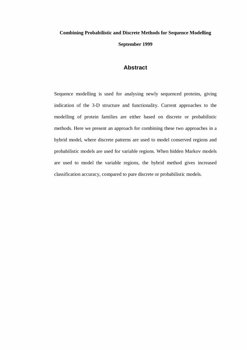
(1998). In figure 2.2 a visualisation of the topology of an HMM can be seen. Each state

transition is given a probability and each match state contains a emission probability for

each of the 20 amino acids.

Delete

Start

Insert

Match

Insert

Delete

Match

Insert

Delete

Match

Insert

End

Figure 2.2. The topology of a hidden Markov model.

When a sequence is aligned to the model it has a path through the model, i.e. each

symbol in the sequence is assigned to a state in the model. The score of the optimal path

through the model is used to indicate how well the sequence fits the specific model. The

8

optimal path is the path through the model that gives the highest probability. The path

itself is a Markov chain where the probability of a state depends only on the previous

state (Durbin et al. 1998).

“An HMM describes a probability distribution over a potentially infinite number

of sequences. Because a probability distribution must sum to one, the ‘scores’ that

an HMM assigns to sequences are constrained. The probability of one sequence

can not be increased without decreasing the probability of one or more other

sequences” Eddy, 1998. Page 756 (original emphasises).

This courses the parameters of an HMM to have non-trivial optima (Eddy, 1998).

Probably the most widely used application of HMMs in molecular biology at the

moment are profile HMMs (Durbin et al. 1998). The HMM in figure 2.2 is an example

of a profile HMM. Profile HMMs are based on multiple alignments of the families they

are to model and therefore need to account for inserts and deletes (diamonds and circles

respectively in figure 2.2). The probability parameters can then be derived directly from

the alignment1.

2.3 Problem Statement

In this thesis the problem investigated is how to create a hybrid modelling method, with

both discrete and probabilistic components, that ideally should incorporate the

advantages of both. To be successful, the hybrid modelling method must be an

improvement from both pure discrete and pure probabilistic methods. In other words

“the best of both worlds”.

1 Interested readers are referred to Durbin et al., 1998 for a very good in-depth description of HMMs for

sequence analysis in bioinformatics.

9

In sequence family modelling the method should have a good ability to identify

members of the modelled family (sensitivity) while at the same time have good ability

to reject those sequences that are not members of the family (specificity).

In this thesis the method is evaluated on protein sequences and compared to other

established methods for generating models for families of protein sequences.

10

3 Related Work

In this chapter the work related to this work is introduced and described.

3.1 PROSITE

The PROSITE (Bucher&Bairoch, 1994) database is the first, largest and most widely

used annotated secondary protein (motif/pattern) database (Attwod, 1997b). PROSITE

consists of a collection of manually constructed patterns, generated by human experts

for a selected motif of each family.

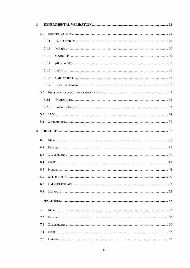
Figure 3.1 The pattern generation process for PROSITE patterns. (© Brigitte

Boeckmann, Ph.D. Reproduced by permission)

If it proves impossible to generate a pattern for a specific family the PROSITE database

has recently included profiles. Profiles are used for modelling families that are hard or

11

impossible to model with patterns (Durbin et al. 1998). Profiles are highly complex

descriptors, generally encoding full sequence length and allowing gap insertions in

generating pairwise alignments between a profile and a target sequence (Attwod et al.

1997). The alignment is done with a dynamic programming method (Bucher, 1997).

The creation of an alignment for every sequence compared to the profile or for every

profile used in analysing a new sequence increases the time and computational power

needed when creating and using the models.

3.2 Pratt

In Jonassen et al. (1995) a pattern discovery algorithm is described that generates

patterns of the same syntax as used in PROSITE. The algorithm uses a depth first search

and uses a block data structure that makes it possible to find very efficiently all

segments of a sequence that match a pattern. Two algorithms to obtain patterns are

given and have been implemented in the Pratt pattern discovery tool.

The tool searches only for patterns that match at least a user specified number of given

sequences, and the discovered patterns are ranked according to a measure of pattern

strength, that is independent of the number of sequences matching the pattern. The score

is defined as a sum of the information content of the pattern positions and a penalty for

flexibility is subtracted.

One of the things that separate this method from other pattern generation methods is

that it does not rely on a multiple alignment as a starting point. The method requires a

number of initial parameters to be set for each run that in most cases need to be

experimentally decided, which can make comparisons made to this method a matter of

dispute as parameters might have been set differently.

12

This method has been shown to be able to discover useful patterns for some protein

families and a pattern discovered by Pratt for the SNAKE_TOXIN family has been

included in the PROSITE database (Jonassen, 1996a).

3.3 IDENTIFY

In Nevill-Manning et al. (1998) a systematic method for determining sequence motifs

from aligned sets of sequences is presented. This method is called EMOTIF (Nevill-

Manning et al. 1998) and it generates as many motifs as possible over a wide range of

sensitivity and specificity. As a result, the method can generate extremely specific

motifs, as well as more sensitive motifs that characterise different subsets of a protein

family. By combining the highly specific motifs in a disjunction, a family can be

described (or modelled) with both high specificity and sensitivity (Nevill-Manning et al.

1998).

The motifs generated are on regular expression form, as in PROSITE patterns.

However, in some cases one or more mismatches are allowed. A statistical analysis was

done of the BLOCKS (Henikoff et al.1995) database and the HSSP database

(Sander&Schneider, 1991), that contain short ungapped highly conserved regions and

global alignments of sequences based on structural alignments, respectively. This

analysis revealed twenty substitution groups that were conserved empirically in both

databases. These substitution groups were used to define the space of motifs available to

model a protein family (Nevill-Manning et al. 1998). In stead of using only the

observed amino acids this method chooses from those substitution groups which are

compatible with the observed amino acids. The algorithm generates all possible motifs

using the allowable substitution group. This has the advantage of identifying

subfamilies with more specific motifs, the subfamilies can then be combined in a

disjunction giving both good coverage and sensitivity (Nevill-Manning et al. 1998).

13

A database called IDENTIFY containing over 50 000 motifs with varying specificity’s

has been constructed using EMOTIF (Nevill-Manning et al. 1998).

3.4 Prints

The PRINTS database is a compendium of protein motif fingerprints, i.e. groups of

aligned, unweighted sequence motifs (Attwood et al. 1997). The fingerprints are defined

and refined with database scanning. Fingerprints are sets of motifs used to predict the

occurrence of a similar motif in either a sequence or a database (Attwood, 1999).

“The fingerprinting method relies on the fact that, in any protein family, only

parts of the sequence are held in common – these usually relate to the key

functional regions or to the core structural elements of the fold.” Attwod, 1999.

Section 1.3

As in most motif finding methods, the method for generating PRINTS fingerprints starts

with a multiple sequence alignment, and from this alignment motifs are derived and

then used in independent database scans. The scans result in one hit-list for each motif,

and the hit-lists are analysed to determine which sequences in the database have

matched all elements of a fingerprint and which have only matched part of it. The

additional sequence data is then used to refine the motifs and the procedure is repeated

until the set of sequences matching all motifs in a fingerprint does not change

(convergence).

3.5 MAMA

In Olsson&Laurio, 1998 a method referred to as MAMA (identify Motifs by Analysis

of Multiple Alignments) is described. As in EMOTIF, this method uses a multiple

alignment as input. Currently the alignments used are the seed alignments from the

14

Pfam database (Sonnhammer et al, 1997). The alignments are analysed by AMA

(Analysis of Multiple Alignments) that generates an entropy profile. The entropy profile

is used to detect motifs that are conserved in the family and are therefore potential

pattern elements. AMA uses a Dirichlet mixture prior to take into account biological

domain knowledge. It has been shown that the use of this prior information improves

the degree of generalisation in probabilistic models of small samples of protein

sequence data (Karpus, 1995, Sjölander et al. 1996).

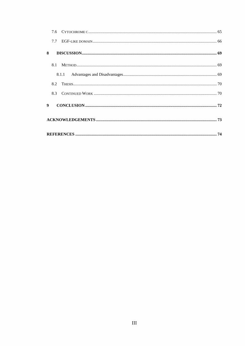
P F A M S W I S S P R O T

PFAM seedalignment

AMAC-x(2,4)-CC-V-x(1,3)-CC-V-x(1,3)-C-x(2,4)-HC-V-x(0,2)-A-C-x(2,4)-HC-V-x(0,2)-A-C-x(1,3)-A-HG-x(2,3)-C-V-x(0,2)-A-C-x(1,3)-A-H

C-REX

Count of false hits

Select the mostgeneral patternhaving no false

positives

C-V-x(0,2)-A-C-x(2,4)-H

Generalize (G-REX)

C-V-x(0,3)-[AG]-C-x(1,4)-[HK]

T-REX

Entropyprofile

Figure 3.2. Overview of the pattern generation method.

Using the information in the entropy profile, C-REX (Creating Regular EXpressions)

creates initial patterns by taking the most conserved columns and adding wildcards

between those. More elements are gradually added, creating a list of patterns (see figure

3.2) and these patterns are tested on the SWISSPROT database, counting false positives

and false negatives. The most general pattern of those that have no false positives is

15

then chosen and it is generalised even more while not allowing any increase in the

number of false positives.

3.6 Combination of Probabilistic and Discrete Motifs

As can be seen in the related work introduced here, until now no-one has investigated

the implication of the combination of probabilistic and discrete motifs such as the

combination of patterns and HMMs. This makes this investigation an important

contribution to the field of sequence analysis.

16

4 Method

In this chapter the hypothesis and the suggested methods, with which the hypothesis can

be tested, are introduced.

4.1 Hypothesis

In a sequence alignment it is common to find several motifs that characterise the aligned

family. It makes sense to use as many as possible or all such conserved regions to build

a family signature (Attwod et al. 1997). It has been shown that for at least certain

protein families2 the disordered regions are involved in the formation of a molecular

complex. It is also reasonable to believe that the parts of the protein that are not similar

enough within the family to be identified as a motif, must have some specific

characteristics in order for the protein to fold into the correct three-dimensional

structure.

Therefore it can be said that motifs are not the only important attributes giving a protein

family a specific function. The parts of the protein that are not found to have clear

sequence similarity with other members of the family are most likely still required to

have specific properties in order for the protein to e.g. fold correctly. For example if a

part of the protein sequence has many hydrophobic residues then that part is most likely

hidden inside the folded protein. These parts might have too low sequence similarity to

be modelled with discrete methods, which means that a probabilistic method must be

used. This argumentation leads to the following sequence of hypotheses, given from the

2 Interested readers are referred to Dunker et al. 1998 where the calmodulin (CaM) target region of

calcineurin (CaN) is investigated.

17

weakest to the strongest (Figure 4.1 shows a visualisation of the different

hypothesises.):

1. Given a generalised pattern, building a hybrid model by replacing wildcards with

probabilistic models will improve the accuracy of the pattern.

2. The hybrid model will have better accuracy than the original pattern(i.e. the pattern

before generalisation).

3. The hybrid model will have better accuracy than both pure discrete and pure

probabilistic methods.

By accuracy in the above text we mean higher sensitivity and specificity, i.e. better at

matching (or identifying) the members of the family and at the same time better at

rejecting non-members found in the database (see section 5.4).

2 and 31

Pure pattern

General ised pattern

Hybrid

General isat ion

Adding probabil ist icelementsImproves

Improves

Improves

3

Pure probabil ist ic

Figure 4.1 Visualisation of the different hypothesis. Pure pattern, Pure

probabilistic, Generalised pattern and Hybrid are the different models. The

numbered arrows show which improvements are expected in the different

hypotheses (the number shows which hypothesis part).

18

4.2 General method

The methods are based on patterns that are generalised to cover the entire family at the

cost of accepting some sequences that are not members of the family.

The idea is that the probabilistic wildcards will identify the false positives, resulting in

an improvement of the specificity of the pattern while still providing the speed of the

pattern search and the biological relevance implicit in the patterns. The suggested model

syntax is based on the method presented in Jonassen et al.(1996) for representing

patterns, where a pattern of length p is written on the form:

A1-x(i1,j1)-A2-x(i2,j2)-…-x(ip-1,jp-1)-Ap

where A1,…,Ap are non-empty sets of symbols, and i1 ≤ j1, i2 ≤ j2,…,ip-1 ≤ jp-1 are non-

negative integers. Each x represents a wildcard region (see section 2.2.1) that can be

replaced by a probabilistic model. The representation suggested here is to index the

wildcards and generate a probabilistic pattern for each one. Matching is then done with

a two-phase method where the pattern is first aligned to the sequence and either

accepted as a hit or rejected if the sequence does not fit the pattern. This first phase

reduces the search space of the second phase to only sequences very similar to the

family. The second phase scores each sequence that the first phase accepted, the score

depends on how well the wildcard region of the sequence matches the probabilistic

models for the wildcards.

The wildcards can be of different lengths ranging from one or two symbols to very long.

To formalise the selection of wildcards for the probabilistic modelling part, some ad hoc

decisions had to be made, based on experimenting with the method.

When the wildcard maximum length is less than 15 symbols it is assumed to be a part of

the discrete motif and not used to generate a probabilistic model. This is done in order

to make sure that the regions used for generation of probabilistic models include enough

19

observations to support a general analysis. Another method for ensuring enough

observations could be to count the number of symbols in the region of the alignment

that corresponds to the wildcard being modelled. If, for example, the number of

sequences in the alignment is more than 100, the size of the wildcard would only need

to be 3 symbols.

If the use of internal wildcards does not give optimal accuracy then a flanking model is

used (see section 4.7). Finally if flanking model do not give optimal accuracy either

then summing the scores of the wildcards is tested and used if it gives better accuracy

than the individual wildcards (see sections 4.5 and 4.6).

4.3 Combination

Here follows a general description of the whole method and the general combination

algorithm.

4.3.1 Generating a Model

The model generation process can be seen in figure 4.2.

20

Pattern generat ion

Probabi l is t ic modelgenerat ion

Pattern

Probabi l is t icmodels

Al ignmentparts

Mul t ip lea l ignment

Hybr id model ofthe protein family

Figure 4.2. Generating a model for a protein family

The model generation process consists of two major steps. First a pattern is generated

for the protein family from a multiple alignment. Then the parts of the alignment that

correspond to the large wildcards of the pattern are each in turn fed to the module for

generating probabilistic models where each wildcard region gets its own probabilistic

model. Putting these parts together results in a hybrid model that contains both the

regular expression from the pattern and, for each wildcard, a corresponding probabilistic

model.

21

4.3.2 Model Use

The intended use of this method is for analysing unknown sequences in order to

determine their family membership. When an unknown sequence is being analysed by

using this method it is first compared to the regular expressions of all family models in

the database. For those patterns that match the sequence, the parts of the sequence that

align to the wildcards of the pattern are compared to the probabilistic models for those

wildcards. The probabilistic models give numerical values providing information of

how well the sequence fits the model. The process is illustrated in figure 4.3.

Regularexpress ioncheck

Unknown sequence

Model database

0/1

Probabi l is t ic model evaluat ion

Num va lue

Sequence parts

Figure 4.3 Analysing an unknown sequence with a database of hybrid models

22

In the following section each step of the model generation process is described in more

detail. The pattern generation algorithm will be described first, and then two

probabilistic modelling methods.

4.4 Pattern Generation

The pattern generation method is kept simple: A pattern from MAMA or PROSITE is

chosen based on which has the lowest number of false negatives. Then the

generalisation procedure continues as follows:

1 Expand the flexibility of a wildcard by first increasing the maximum length in

steps of one until no improvement is made. Then the maximum length is

increased by 20 and if that gives no improvement the max length is restored to

the last value that made improvement. Then the same procedure is repeated for

the minimum, decreasing in step of one until no improvement is made and then

stop if no improvement is made by decreasing by 20 (or to zero if the minimum

length is less than 20). If this decreases the number of false negatives then keep

the expanded wildcard. Otherwise go back to the wildcard before the change.

2 Repeat step 1 until no more improvement is found by expanding any wildcard.

3 Starting with the elements having the largest number of amino acids, the

elements having more than 8 amino acids are removed one at a and the

wildcards on each side are combined into one. If removing an element decreases

the number of false negatives then the change is kept, otherwise the element is

reinserted.

4 Repeat step 3 until no more improvement is found.

5 If there are still any false negatives then those sequences are first aligned to the

Pfam seed alignment for the family and then manually aligned to the pattern.

Then the pattern is generalised manually to include the last false negatives.

23

If the number of false negatives reaches zero in any step, then the process is stopped and

the current pattern is returned as solution.

Step 5 is used for particularly difficult families the pattern is aligned to the sequences

that are still false positives after the process described above, then the alignment can be

used to guide the generalisation to make the changes needed for the final sequences.

4.5 Probabilistic Models Based on Distribution Analysis

The suggested notation for models replacing wildcards with simple probabilistic models

is:

A1- x1(i1,j1,m1) -A2- x2(i2,j2,m2)- …-xp-1(ip-1,jp-1,mp-1)- Ap

where mk is a vector with the distribution information needed to match the sub-sequence

for the wildcard region to the model it represents. The sub-sequences of the accepted

sequences are scored with the distribution model for the wildcard in question. This

assigns the accepted sequences a value that can be used to identify false positives by

rejecting sequences that score below a specific threshold value.

The distribution analysis determines the frequency of each amino acid (symbol) in the

region of the alignment that corresponds to the wildcard. This can be done by simply

counting the instances of each amino acid in the wildcard region of the multiple

alignment. It is then straightforward to calculate the percentage for each of the twenty

amino acids and store them in the vector for the wildcard. This distribution analysis,

where only the frequency of one symbol occurring at a time is done, can be replaced

with one where the frequency for a specific sub-sequence of symbols is used instead of

single symbols (e.g. A’s followed by V’s or F’s followed by E’s and then D’s). This can

be done with basically the same method but with an n-dimensional vector, where n is

the number of symbols in the sub-sequence used in the analysis. This however would

only work if the wildcard is very large and if there are many sequences in the alignment,

24

otherwise the amount of information implicit in the wildcard does not support such an

analysis.

Another problem with the use of probabilistic models as described above is how to

combine the results from the models for each wildcard sequence part. One possible

solution is to let each wildcard get equal fraction of the final numerical value, another

is to make the length of the region determine the share of the final value. It could even

be beneficial to ignore the lowest scoring wildcard and use the ones with higher scores.

In this thesis the size of the wildcard is used to determine the share it gets in the final

score. However when the system is functional it is not hard to change the calculation to

test other methods, but that analysis is left to future work.

4.6 Hidden Markov Models

The method presented in the previous chapter might be too general. It might be enough

to use a method that represents a more restrictive grammar. Hidden Markov models

encode a stochastic regular grammar and have been used with good results in sequence

family modelling. Therefore comparison will be made to a similar method using HMMs

to model the wildcard regions. The representation of such hybrid models can be written

as follows:

A1- x1(i1,j1,M1)- A2- x2(i2,j3,M2)-… -xp-1(ip-1,jp,Mp-1)-Ap

with the same definitions as above and the addition of the many, but relatively small,

hidden Markow models Mn. This will be done with the same two-pass method as in

previous section. Each HMM part is generated with Sequence Alignment and Modelling

system (SAM) which is a collection of flexible software tools for creating, refining, and

using linear hidden Markov models for biological sequence analysis (Hughey et al.

1996).

25

To train the HMMs the sequence parts of the alignment that are covered by the wildcard

are cut out and fed to SAM. To speed up SAM training it can take an alignment instead

of individual sequences, as the sequence parts cut from the alignment are already

aligned. Another way to generate the HMM would be to generate a model for the whole

alignment and the parts of the model that correspond to the discrete motif can be

removed or changed so as not to influence the results. The problem is however to locate

the parts of the HMM that correspond to a specific column in the alignment since in the

HMM the column can be represented in different model parts as SAM can change the

alignment while training the model.

In the distribution analysis the summation of the different models to give one result

value was a problem as it could be dependent on the number of models. This is not a

problem with HMMs. HMM scoring is based on logarithms that can be summed up

without the number of HMM’s in the hybrid model affecting the results (Durbin et al,

1998).

4.7 Flanking Models

For some protein families the pattern does not contain wildcards large enough to use in

probabilistic analysis. For these families there is a need to find some other way to

include the probabilistic aspect in the model.

Here the solution is to use probabilistic models for the sequence parts flanking the area

that is covered by the pattern. The suggested syntax extension is as follows:

• For distribution analysis:

mo-A1- x1(i1,j1,m1) -A2- x2(i2,j2,m2)- …-xp-1(ip-1,jp-1,mp-1)- Ap-mp

• For HMM:

M0-A1- x1(i1,j1,M1)- A2- x2(i2,j3,M2)-…-xp-1(ip-1,jp,Mp-1)-Ap-Mp

26

In the above, mi is used to represent a probabilistic model derived by distribution

analysis, and Mi is used to represent an HMM. The flanking models are represented by

m0 and mp for distribution analysis and M0 and Mp for HMMs.

Restrictions on the lengths of the flanking sequences in the seed alignment are not used

in matching sequences to patterns.

4.8 Cut-off

To decide the cut-off value the following method is used.

The first case is when there is a separation between all false positives and all true

positives of the sequences matching the generalised pattern. This means that the highest

scoring true positive (Tmax) has lower score than the lowest scoring false positive (Fmin).

In this case the cut-of value is set to the mean value of Tmax and Fmin, i.e. 2

minmax FT +.

The second case is when there is an overlap between the scores of false positives and

true positives. In this case an algorithm does an linear starting with zero and searching

for an cut-of giving the lowest number of false positives and false negatives.

4.9 Evaluation of the Method

When evaluating a new method it is important to identify its strengths and weaknesses.

Therefore the families used in the evaluation need to be from a variety of families with

different properties, i.e. different number of members, different lengths, and different

levels of similarity (identity). The selected families need to vary from families known to

be easy to model to infamous families that have proven hard or impossible to model

with other methods.

In the comparison to other methods is important to know if the hybrid method really

gives “the best of both worlds” or if it only does as well as using probabilistic methods

27

or only discrete methods alone. Therefore it is necessary to compare to methods for

generating patterns, such as MAMA, and also to probabilistic methods such as HMMs.

In the comparison to the other methods it is necessary to use the same data in the

experiments with the different methods, so that an error in a database entry has the same

effects on all methods. This requires that the methods can be run on a local database,

both when creating a model and when testing the models. For these reasons the methods

selected for comparison are MAMA as an automatic pattern generation method, and

SAM as an HMM generation method. The requirement of the local test database

excludes Pfam which is a method based on HMMs generated from automatically and

manually constructed seed alignments.

The oldest and most used pattern database is PROSITE (Bucher&Bairoch, 1994), which

contains manually constructed patterns for protein families and is often used for

comparison when introducing new methods for constructing models for protein

families. For this reason the PROSITE patterns are also used in the following

experiments to have a common comparison to other current and future methods.

Pratt, Prints and even EMOTIF would also be relevant the comparison to these methods

is left for future work. This comparison should be done in the future if the results of this

project are promising.

28

5 Experimental Validation

In this chapter the families chosen for validating the method are briefly presented and

thereafter the tools and implementations used in the experiments are introduced and

described.

5.1 Protein Families

The database used in the experiments is Swissprot version 35. In the Swissprot

documentation the family membership, if known, is included as well as if the complete

sequence is given or just a fragment of it.

The MAMA method generates patterns that can correspond to different motifs in an

alignment of a protein family (see figure 5.1), for this reason the sequence fragments are

ignored found in the database are ignored.

PROSITE

PRINTS

M A M A

Figure 5.1 Comparison fo how patterns from PROSITE, PRINTS and MAMA

correspond to the motifs in a multiple alignment.

The families were selected based on manual inspection of their sequence characteristics

with the primary concern of validating the method on families with varying levels of

modelling complexity. No family was selected based on functional characteristics. The

families chosen were:

29

• 14-3-3

• Kringle

• Crystallins

• PfkB

• Insulin

• Cytochrome c

• EGF-like domain

Here follows a description of the chosen families, the descriptions are based on the

documentation in PROSITE release 15 and on the Pfam version 4.1 documentation. All

credits are therefore to the hardworking people that created and maintain these

databases. For each family the statistics from Pfam are given, that is, average length,

and average % identity. The average length needs no explanation but the average %

identity is calculated as follows: Given that a family has N sequences it has 2

)1(* −NN

pairs of sequences. The identity for each pair is calculated as the number of identical

residues divided by the length of alignment and the average for all pairs is taken. (Erik

Sonnhammer, personal communication).

5.1.1 14-3-3 Proteins

A family of closely related acidic homodimeric proteins which were first identified as

being very abundant in mammalian brain tissues and located preferentially in neurons.

The proteins of this family seem to have multiple biological activities and play a key

role in signal transduction pathways and the cell cycle. They interact with kinases such

as PKC or Raf-1; they seem to also function as protein-kinase dependent activators of

tyrosine and tryptophan hydroxylases and in plants they are associated with a complex

that binds to the G-box promoter elements. Members of the 14-3-3 family of proteins

30

are ubiquitously found in all eukaryotic species studied and have been sequenced in

fungi, plants, Drosophila, and vertebrates. The sequences of this family of proteins are

extremely well conserved (PROC00633). According to the Pfam documentation

(http://www.sanger.ac.uk/cgi-bin/Pfam/getacc?PF00244) the average length is 212.3

amino acids and the average identity is 69%. PROSITE pattern has full sensitivity and

specificity, so it picks up all family members while rejecting all non-members. This

family should therefore be easy to model and is used as an example of a family that is

can be modelled with a standard pattern.

5.1.2 Kringle

These are triple-looped, disulfide cross-linked domains found in a varying number of

copies, in some serine proteases and plasma proteins. Kringle domains are thought to

play a role in binding mediators, such as membranes, other proteins or phospholipids,

and in the regulation of proteolytic activity (PROC00020). In the Pfam documentation

the average length of 78.4 amino acids is given, and the average identity is 48%. This

makes this family a harder one to model but methods based on patterns still do a

relatively good job, e.g. for the PROSITE pattern there are 4 false positives and no false

negatives.

5.1.3 Crystallins

Crystallins are the dominant structural components of the eye lens. Among the different

types of crystallins, the beta and gamma crystallins form a family of related proteins.

Structurally, beta and gamma crystallins are composed of two similar domains which, in

turn, are each composed of two similar motifs with the two domains connected by a

short connecting peptide. Each motif, which is about forty amino acid residues long, is

folded in a distinctive “Greek key” pattern (PROC00197). The number of none

31

fragment members of this family in the database used is 66, the pfam seed alignment

length is 94 amino acids. The average length is 81.7 and average identity is 39%

according to pfam documentation on the Crystallins family. This family seems to give

PROSITE a hard time as it has 236 false positives and no false negatives. This can

however have other explanations than that the method is hard to model with patterns as

the MAMA method generates pattern with no false positives and 3 false negatives.

5.1.4 pfkB Family

It has been shown (Wu et al. 1991, Orchard et al. 1990, Blatch et al. 1990) that a group

of carbohydrate and purine kinases are evolutionary related and can be grouped into a

single family, which is known as the 'pfkB family' (Wu et al. 1991).

All those kinases are proteins of from 280 to 430 amino acid residues that share a few

regions of sequence similarity (PROC00504). In the Pfam documentation the family has

average length of 128.9 amino acids and average identity of 25%. This low identity

makes members of the family hard to separate for random hits in the large sequence

databases available and the modelling is therefore hard.

5.1.5 Insulin

The insulin family of proteins groups a number of active peptides, which are

evolutionary related. They all share a conserved arrangement of four cysteines in their A

chain. The first of these cysteines is linked by a disulfide bond to the third one and the

second and fourth cysteines are linked by interichain disulfide bonds to cysteines in the

B chain (PROC00235). According to the Pfam documentation the average length is 68.4

amino acids and average identity is 45%. Having such short sequences should strain the

method as it requires adequately long wildcards to build the probabilistic part base

enough information.

32

5.1.6 Cytochrome c

In proteins belonging to the cytochrome c family, the heme group is covalently attached

by thioether bonds to two conserved cysteine residues. The consensus sequence for this

site is Cys-X-X-Cys-His and the histidine residue is one of the two axial ligands of the

heme iron. This arrangement is shared by all proteins known to belong to cytochrome c

family (PROC00169). This family is infamous for being very hard to model and is

therefore often used to evaluate the new methods. This and the following family are

chosen to test the limits of the method. According to the Pfam documentation the

average length is 93.1 amino acids and average identity is only 28%.

5.1.7 EGF-like domain

A sequence of about thirty to forty amino acids long which is found in the sequence of

epidermal growth factor (EGF) has been shown to be present, in a more or less

conserved form in a large number of mostly animal proteins.

The functional significance of EGF domains in what appears to be unrelated proteins is

not yet clear. Although, a common feature seems to be that these repeats are found in

the extracellular domain of membrane-bound proteins or in proteins known to be

secreted (exception: prostaglandin G/H synthase) (PROC00021). In the pfam

documentation the average length is given to be 34 amino acids and average identity

34%. The family has a very large variation in length, which may make it very hard to

model with the method described in this work.

33

5.2 Implementation of the hybrid method

In the implementation of this method two other tools have been used.

5.2.1 Discrete part

Firstly some parts of the method are based on the MAMA method. The script used to

test the generated pattern is the same as T-REX in the MAMA method. Also the

implementation of the alignment of an unknown sequence to a pattern uses the

transcription of patterns part of T-REX. One small script for additional database

extraction is also used in testing the method. These scripts are written by Bjorn Olsson

at the University of Skövde, Sweden.

5.2.2 Probabilistic part

The method can use any HMM generation and scoring program. The program package

chosen in this work is the SAM (Hughey et al. 1996, Krogh et al. 1994, Hughey&Krogh

1996). The Sequence alignment and modelling system is a collection of software tools

for creating, refining and using HMM in biological sequence analysis (Hughey et al.

1996). In SAM the model estimation is done with the forward-backward algorithm, also

known as the Baum-Welch algorithm, which is described in Rabiner (1989). It is an

iterative algorithm that maximises the likelihood of the training sequences. To prevent

over-fitting on the training data regularises based on Dirichlet distributions is used

(Hughey&Krogh 1996). In the HMM comparison both using priors and not using priors

is tested in an attempt to get the best possible model representing probabilistic methods.

An inherent problem in hill-climbing algorithms, like the one used to generate the

HMM model in SAM, is the danger of getting stuck on local maximum. To prevent this

34

the training is restarted with several different initial models and the result with highest

likelihood is selected (Hughey&Krogh 1996).

To align sequences to the model the Viterbi algorithm (Rabiner, 1989), that can find the

best alignment and its probability without going through all the possible alignments, is

used. When alignment is already known then a tool called “modelfromalign” can be

used to create a HMM directly from the alignment. If a trustworthy, manually created,

alignment is available then this is often the best way to build a model (Hughey et al.

1996). The HMM for wildcards were devised with this option where the alignment parts

were cut from pfam seed alignments. The seed alignments do not include whole

families so this also gives an estimate of the generaliseability of the resulting models.

5.3 SAM

There are more than one way of creating HMMs using the SAM tool. HMMs can be

created from ready-made alignments or from groups of sequences. The model can be

initiated with priors or with no priors (see previous section), using no priors course the

default single priors to be used. In the experiments the HMMs were created on the Pfam

seed alignments that are the same as used to create the HMMs used in Pfam. Using

priors or not seemed in some cases to make a difference so to avoid excluding some

potentially better models by using either single priors or not then both were done in the

experiments. Those can be seen in table 5.1, where there is one row for SAM with

priors and another for SAM with single priors.

35

5.4 Comparison

The data recorded for the different approaches is the number of false positives and false

negatives. Some sequences in the database are only sequence fragments containing only

parts of the protein sequences, In PROSITE these fragment sequences are included as

PROSITE patterns model only one motif. In MAMA and the hybrid method the pattern

can contain more than one motif so the fragment sequences are ignored in the results.

From these results the sensitivity and specificity can be calculated, which are calculated

as follows:

NegativesPositives

Positives

FalseTrue

TrueySensitivit

+=

PositivesPositives

Positives

FalseTrue

TrueySpecificit

+=

In Burset&Guigó (1996) am measure called Correlation Coefficient (CC), it is used to

give a measure of the accuracy of gene finding programs and is calculated form same

factors as used in calculating sensitivity and specificity. It is arguable that is also has

value in estimating the accuracy of a modelling method for finding members of a

protein family in a large database. CC is calculated as follows:

( ) ( )( ) ( ) ( ) ( )NNPPPNNP

PNNP

FTFTFTFT

FFTTCC

+∗+∗+∗+∗−∗

=

Where TP is True Positives, FP is False Positives, TN is True Negatives, and FN is False

Negatives.

These values are calculated for all methods, including the hybrid method with and

without flanking models. The results for the Hybrid method after removing the

sequences found in the Pfam seed alignment are also presented, these results are marked

36

NS. This gives information on how the method does on sequences that it has not been

trained on, as the probabilistic part is only trained on the seed alignment. These are only

presented for the Hybrid method using HMM as a probabilistic part as the results using

the Distribution Analysis (DA) are very bad.

The results can then be presented in tables as the “blank” one shown below.

FP FN Sens. Spec. CC x(j,i)

PROSITE

MAMA

SAM-priors

SAM-single priors

Generalised pattern

NS Hybrid, HMM

NS Hybrid, fl. HMM

Hybrid with HMM

Hybrid with fl. HMM

Hybrid with DA

Hybrid with flanking DA

Table 5.1 Template for results table.

Wildcards are numbered from left to right and flanking models are not numbered but

marked fl. (see Table 5.1). The wildcards are identified as x followed by the number of

the wildcard (same as in the pattern). The last column shows the size of the wildcard

being modelled in the hybrid method.

37

6 Results

In this chapter the results for each family are described in a separate section.

6.1 14-3-3

The 14-3-3 family pattern generated by MAMA is as follows:

G-x(5)-W-x(1,7)-Q-x(96,101)-P-x(3)-G-x(58)-W

PROSITE gives two patterns, both picking up all members while rejecting all none-

members. Those patterns are:

R-N-L-[LIV]-S-[VG]-[GA]-Y-[KN]-N-[IVA]

and

Y-K-[DE]-S-T-L-I-[IM]-Q-L-[LF]-[RHC]-D-N-[LF]-T-[LS]-W- [TAN]-[SAD]

As can be seen, the MAMA pattern has long wildcards while PROSITE finds patterns

with no wildcards. The hybrid method needs wildcards to work so therefore the

generalised pattern for the 14-3-3 family is based on the pattern generated by MAMA.

After generalisation the pattern had the following appearance (Wildcards used for

probabilistic modelling are in bold letters):

G-x1(5)-W-x2(1,7)-[QG]-x3(96,103)-P-x4(3)-G-x5(58,60)-W

The generalised pattern does not differ much from the original MAMA pattern as it only

needed to be generalised to include one more sequence. The first two wildcards and the

fourth are not changed, the third is increased in maximum length by two as is the last

wildcard. One element is changed, adding Glycine.

The wildcards modelled with probabilistic methods are wildcards 3 and 5, which are the

largest of the available wildcards in this pattern. As can be seen in table 6.1, replacing

the internal wildcards is enough to give full sensitivity and specificity, so flanking

models are not needed.

38

This family has 50 known non-fragment members in the experimental database, 13 of

those are in the Seed alignment.

F. P. F. N. Sens. Spec. CC x(j,i)

PROSITE 0 0 1.00 1.00 1.00

MAMA 0 2 0.96 1.00 0.98

SAM-priors 26 1 0.98 0.65 0.80

SAM-single priors 26 1 0.98 0.65 0,80

Generalised pattern 12 0 1.00 0.81 0.90

NS Hybrid , HMM, x3 0 0 1.00 1.00 1.00 96-103

NS Hybrid, HMM x5 0 0 1.00 1.00 1.00 58-60

Hybrid, HMM x3 0 0 1.00 1.00 1.00 96-103

Hybrid, HMM x5 0 0 1.00 1.00 1.00 58-60

Hybrid, DA x3 2 0 1.00 0.96 0.99 96-103

Hybrid, DA x5 3 3 0.94 0.94 0,94 58-60

Table 6.1 Results for the 14-3-3 family.

To show the quality of the separation between members and non-members the scoring

distribution of the sequences accepted by the generalised pattern are presented in Figure

6.1.

Scoring distribution for HMM wildcard 3

05

10152025303540

-160-180

-120-140

-80-100

-40-60

0-20

4020

8060

Score

FALSE

TRUE

Figure 6.1 Scoring distribution for the HMM created for wildcard 3.

39

6.2 Kringle

MAMA generates the following pattern for the kringle family:

C-x(4)-G-x(2,4)-G-x(6,10)-C-x(2)-W-x(18,28)-C-x(2)-P

PROSITE has both a profile and a pattern for this family. The pattern is as follows:

[FY]-C-R-N-P-[DNR]

The pattern has four false positives and zero false negatives, while the profile has zero

false positives and zero false negatives. The pattern has no wildcards while the MAMA

pattern does have wildcards, though they are rather short. The generalised pattern for

the kringle family is derived from the pattern generated by MAMA. The original

MAMA pattern has zero false positives and one false negative. After generalisation the

pattern has one false positive and zero false negatives. The generalised pattern is as

follows appearance (Wildcards used for probabilistic modelling are in bold letters):

C-x1(4,6)-G-x2(2,4)-G-x3(6,10)-C-x4(2)-W-x5(18,28)-C-x6(2)-P

Here the generalisation is made only by increasing the maximum length of the

wildcards, while the elements are all the same.

The only wildcard that contains enough information to generate a probabilistic model is

the largest i.e. x5(18,28). The right flank is also large enough to create a probabilistic

model so in this family both a wildcard and a flanking models can be examined. The

number of know non-fragment members is 35, 12 of which occur in the seed alignment.

The results are presented in the table below.

40

F. P. F. N Sens. Spec. CC x(j,i)

PROSITE 4 0 1.00 0.91 0.95

MAMA 0 1 0.97 1.00 0.99

SAM-priors 3 0 1.00 0.92 0.96

SAM-single priors 3 0 1.00 0.92 0.96


NS Hybrid, HMM x5 0 0 1.00 1.00 1.00 18-28

NS Hybrid, fl. HMM 0 0 1.00 1.00 1.00 18-27

Hybrid, HMM x5 0 0 1.00 1.00 1.00 18-28

Hybrid, fl. HMM 0 0 1.00 1.00 1.00 18-27

Hybrid, DA x5 1 0 1.00 0.97 0.99 18-28

Hybrid, fl. DA 1 0 1.00 0.97 0.99 18-27

Table 6.2 Results for the krigle family.

Figure 6.2 shows the HMM scoring distribution for the families that match the

generalised pattern for the internal wildcard. Figure 6.3 shows the same for the flanking

models.


02468

101214

-35-40

-30-35

-25-30

-20-25

-15-20

-10-15

-5-10

0-5

50

105

1510

2015

2520

Score

FALSE

TRUE

Figure 6.2 Scoring distribution for HMM wildcard 5.

There is only one false positive for the generalised pattern and the score for that

sequence is very different than the scores of the sequences that belong to the family.

41

Scoring distribution for flanking HMM

0

2

4

6

8

-50-55

-45-50

-40-45

-35-40

-30-35

-25-30

-20-25

-15-20

-10-15

-5-10

0-5

50

105

1510

2015

2520

Score

FALSE

TRUE

Figure 6.3 Scoring distribution for flanking HMM.

6.3 Crystallins

For the Crystalins family the MAMA pattern is as follows:

[DEY]-x(3)-[FHLY]-x-G-x(1,3)-[DEQR]-x(16,22)-S-x(4,5)-[GH]-x-[AFKW]-x(2)-[FLSY]-x(6,7)-

G-x(8,13)-[AFY]-x(11,18)-[AS]-x-[KR]

The PROSITE pattern is:

[LIVMFYWA]-x-{DEHRKSTP}-[FY]-[DEQHKY]-x(3)-[FY]-x-G-x(4)- [LIVMFCST]

The generalised pattern for the Crystallins family is derived form the MAMA pattern

and is as follows appearance (Wildcards used for probabilistic modelling are in bold

letters):

[KRQTE]-x1(3)-[YF]-[KEY]-x3(3)-[FLY]-x4-G-x5(47,55)-[END]-[ALFY]-[PRKST]

Here the generalisation has changed the pattern much, removing elements, enlarging

wildcards, and adding symbols to elements. The pattern after generalisation has 52 false

positives.

The only wildcard large enough to use in generating a probabilistic model is the one

with minimum length of 47 and maximum length of 55. It is also possible to use one

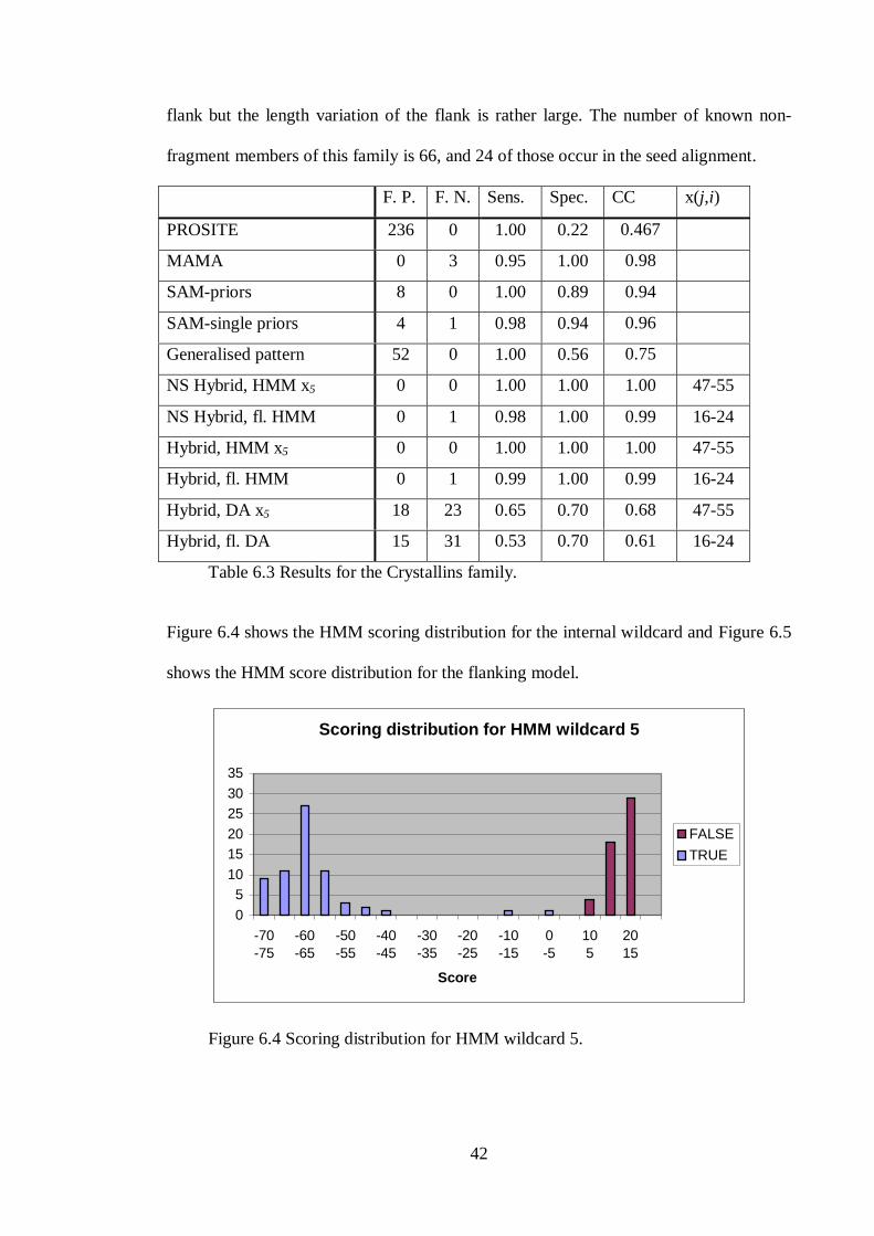
42

flank but the length variation of the flank is rather large. The number of known non-

fragment members of this family is 66, and 24 of those occur in the seed alignment.


PROSITE 236 0 1.00 0.22 0.467

MAMA 0 3 0.95 1.00 0.98

SAM-priors 8 0 1.00 0.89 0.94



NS Hybrid, HMM x5 0 0 1.00 1.00 1.00 47-55

NS Hybrid, fl. HMM 0 1 0.98 1.00 0.99 16-24

Hybrid, HMM x5 0 0 1.00 1.00 1.00 47-55

Hybrid, fl. HMM 0 1 0.99 1.00 0.99 16-24

Hybrid, DA x5 18 23 0.65 0.70 0.68 47-55

Hybrid, fl. DA 15 31 0.53 0.70 0.61 16-24

Table 6.3 Results for the Crystallins family.

Figure 6.4 shows the HMM scoring distribution for the internal wildcard and Figure 6.5

shows the HMM score distribution for the flanking model.


0

510

1520

2530

35

-70-75

-60-65

-50-55

-40-45

-30-35

-20-25

-10-15

0-5

105

2015

Score

FALSE

TRUE


43


0

510

1520

2530

35

50

105

1510

2015

2520

3025

3530

4035

4540

5045

5550

6055

6560

7065

7570

Score

FALSE

TRUE


6.4 PfkB

The pattern generated using MAMA is:

[AG]-G-x(2,3)-[NT]-x-[AMST]-x(1,6)-[AGKSV]-x(9,14)-[AGPS]-x(145,192)-[GP]-x(26,48)-

[AGS]-[AS]-[DG]-D-x(3)-[AGSV]-[AG]

PROSITE gives two patterns for this family:

[AG]-G-x(0,1)-[GAP]-x-N-x-[STA]-x(6)-[GS]-x(9)-G

and

[DNSK]-[PSTV]-x-[SAG](2)-[GD]-D-x(3)-[SAGV]-[AG]- [LIVMFYA]-[LIVMSTAP]

As with the previous families the pattern the MAMA pattern is generalised. The

generalisation results in the following pattern:

[AGN]-[GS]-x2(2,3)-[NTA]-x3(1,2)-[AMST]-x4(1,6)-[AGKSV]-x5(9,20)-[AGPS]-x6(172,228)-

[AGS]-[AS]-[DG]-D-x10(3)-[AGSV]-x11(0,3)-[AG]

Changes of the pattern in generalisation are in the form of increased flexibility of

wildcards, added symbols in the elements, and in removing elements and combining the

wildcards on either side.

44

The wildcards used are the one with length variation 9 to 20 and the largest allowing

172 to 228 residues. The pattern covers all of the Pfam seed alignment so no flanking

model could be included in the investigation of this family. The non-fragment members

of the PfkB family are 36, of which 22 occur in the seed alignment.


PROSITE 24 14 0.61 0.48 0.54

MAMA 0 7 0.81 1.00 0.90

SAM-priors 6 0 1.00 0.86 0.93



NS Hybrid, HMM x5 2 9 0.36 0.71 0.51 9-20

NS Hybrid, HMM x6 1 1 0.93 0.93 0.93 172-228

NS Hybrid, x5 + x6 0 1 0.93 1.00 0.96 9-20

172-228

Hybrid, HMM, x5 2 9 0.79 0.94 0.84 9-20

Hybrid, HMM, x6 1 1 0.97 0.97 0.97 172-228

Hybrid, x5 + x6 0 1 0.97 1.00 0.99 9-20

172-228

Hybrid, DA x5 14 32 0.11 0.22 0.16 9-20

Hybrid, DA x6 3 34 0.06 0.40 0.15 172-228

Table 6.4 Results for the PfkB family.

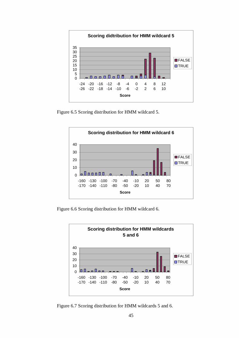
45

Scoring didtribution for HMM wildcard 5

05

101520253035

-24-26

-20-22

-16-18

-12-14

-8-10

-4-6

0-2

42

86

1210

Score

FALSE

TRUE



0

10

20

30

40

-160-170

-130-140

-100-110

-70-80

-40-50

-10-20

2010

5040

8070

Score

FALSE

TRUE


Scoring distribution for HMM wildcards 5 and 6

0

10

20

30

40

-160-170

-130-140

-100-110

-70-80

-40-50

-10-20

2010

5040

8070

Score

FALSE

TRUE

Figure 6.7 Scoring distribution for HMM wildcards 5 and 6.

46

6.5 Insulin

The pattern generated by MAMA is:

C-x(4)-[AIV]-x(6,7)-[CT]-x(11,123)-C-[CT]-x(3)-C-x(6,8)-LQVY-C

The pattern used in PROSITE is:

C-C-{P}-x(2)-C-[STDNEKPI]-x(3)-[LIVMFS]-x(3)-C

The pattern used for generalisation here is also constructed by the MAMA method.

After generalisation the pattern is as follows appearance (Wildcards used for

probabilistic modelling are in bold letters):

C-x1(4)-[AIVG]-x2(6,7)-[CT]-x3(11,123)-C-[CT]-x5(3)-C-x6(6,8)-[LQVYAF]-C

The generalisation does not have to change the pattern much to get full sensitivity, all

wildcards are the same and only two elements have been changed.

Here no flanking model could be created. The wildcard most likely for results is the

largest but the problem is that the flexibility of the wildcard is very large, from 11 to

123 residues. The number of sequences in this family is very large and in the seed

alignment there are 43 sequences. This makes it possible to use smaller wildcards to

generate probabilistic models. To investigate this idea all the 5 non-empty wildcards

were modelled.

There are 143 know non-fragment members in this family, of which 43 occur in the

seed alignment.

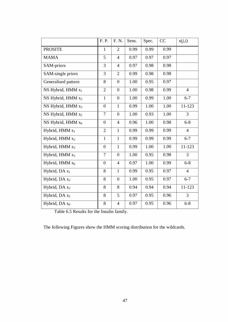
47


PROSITE 1 2 0.99 0.99 0.99

MAMA 5 4 0.97 0.97 0.97

SAM-priors 3 4 0.97 0.98 0.98



NS Hybrid, HMM x1 2 0 1.00 0.98 0.99 4

NS Hybrid, HMM x2 1 0 1.00 0.99 1.00 6-7

NS Hybrid, HMM x3 0 1 0.99 1.00 1.00 11-123

NS Hybrid, HMM x5 7 0 1.00 0.93 1.00 3

NS Hybrid, HMM x6 0 4 0.96 1.00 0.98 6-8

Hybrid, HMM x1 2 1 0.99 0.99 0.99 4

Hybrid, HMM x2 1 1 0.99 0.99 0.99 6-7

Hybrid, HMM x3 0 1 0.99 1.00 1.00 11-123

Hybrid, HMM x5 7 0 1.00 0.95 0.98 3

Hybrid, HMM x6 0 4 0.97 1.00 0.99 6-8

Hybrid, DA x1 8 1 0.99 0.95 0.97 4

Hybrid, DA x2 8 0 1.00 0.95 0.97 6-7

Hybrid, DA x3 8 8 0.94 0.94 0.94 11-123

Hybrid, DA x5 8 5 0.97 0.95 0.96 3

Hybrid, DA x6 8 4 0.97 0.95 0.96 6-8

Table 6.5 Results for the Insulin family.

The following Figures show the HMM scoring distribution for the wildcards.

48


01020304050607080

-9,5-10

-8-8,5

-6,5-7

-5-5,5

-3,5-4

-2-2,5

-0,5-1

10,5

2,52

Score

FALSE

TRUE



0

10

20

30

40

50

60

-13-14

-11-12

-9-10

-7-8

-5-6

-3-4

-1-2

10

32

54

Score

FALSE

TRUE


49

Scoring distribution fo HMM wildcard 3

020406080

100120140160

-160-170

-130-140

-100-110

-70-80

-40-50

-10-20

2010

5040

8070

Score

FALSE

TRUE



05

10152025303540

-3,5-4

-3-3,5

-2,5-3

-2-2,5

-1,5-2

-1-1,5

-0,5-1

0-0,5

0,50

10,5

1,51

21,5

2,52

score

FALSE

TRUE


50


05

1015202530

-12-12,5

-10,5-11

-9-9,5

-7,5-8

-6-6,5

-4,5-5

-3-3,5

-1,5-2

0-0,5

1,51

Score

FALSE

TRUE


6.6 Cytochrome c

Finding a pattern to generalise for this family was a difficult problem as pattern

generation methods that were tried did not produce effective patterns and in

generalisation the number of false positives increased quickly to include half the test

database. The MAMA method generates following pattern:

[AEGIKLMRTV-AFILQTYSN]-x(1,4)-C-[AEGIKLMSTVYHQN]- [AGHIKLMQSTVE]-C-H-

x(2)-[ADEGHIKNQTVRW]-x(2,25)-[AEGKLMPQSTVW]-x(2,3)-[ADEGKNPST]-x(5,24)-

[FHIKLMRSV]-x(2,4)-[AGHIKLRTVY]-x(8,27)-[AFGHILMNPQVWY]-x(5)-[ADEGKPQRSTV]-

x(1,5)-[ADEGIKLNQRSVYW]- [AILMVP-AEILSTVWYFH]-[ADEGKLNQT]-[FHWY]-

[FILMVYD]-x(1,12)-[AFIKLMNQRSTV]

PROSITE on the other hand gives this pattern:

C-{CPWHF}-{CPWR}-C-H-{CFYW}

In Lund et al. (1998) there is a comparison of modelling with ClustalW and HMM, and

there a pattern is retrieved for the cytochrome c family from a ClustalW multiple

alignment that gives good results. The pattern is derived directly from a ClustalW

51

multiple alignment of the Cytocrome c family and in Lund et al. (1998) it gives as good

results as using HMM. The original pattern is (Dan Lund, personal communication):

[ARNDQEHLKMPST]-[ANDCEGHILKMPSTV]-[AILKFYV]-

[ARNDCQEGHILKMFPSTWYV]-x(1,29)-[C]-[ANDCQEGHILKMFPSTYV]-

[ANDCQEGHILKMPSTYV]-[C]-[H]-[ANDCQEGHILKMFPSTYV]-x(2,491)

This pattern is generalised and still gives quite a number of false positives but still is the

best that could be achieved in a number of different attempts. The generalised pattern is

appearance (Wildcards used for probabilistic modelling are in bold letters):

[ARNDQEHLKPST]-[ADEGHILKPST]-[ALFYV]-x3(3,12)-[CAF]-x4(2)-C-H

It is noteworthy that the pattern does not have any large wildcards. This makes the

probabilistic part of the method run into difficulties, as there is no internal wildcard to

build a model on. The flanking edges are also of much length variation, but in an

attempt to get more material to build probabilistic part on the right flank is modelled

also.

In the test database the family has 288 known non-fragment members, of which 44

occur in the seed alignment.

52


ClustalW 510 12 0.96 0.35 0.58

PROSITE 404 6 0.98 0.42 0.63

MAMA 4 109 0.62 0.98 0.78

SAM-priors 15 87 0.70 0.93 0.81



NS Hybrid, HMM x3 46 231 0.05 0.22 0.11 3-12

NS Hybrid, fl. HMM 42 36 0.85 0.83 0.84 60-121

Hybrid, HMM x3 46 269 0.07 0.29 0.14 3-12

Hybrid, fl. HMM 42 40 0.86 0.86 0.86 60-121

Hybrid, DA x3 49 278 0.03 0.17 0.08 3-12

Hybrid, fl. D.A 144 250 0.13 0.21 0.16 60-121

Table 6.6 Results for the Cytochrome c family.


050

100150200250300350400

-5-5,5

-4-4,5

-3-3,5

-2-2,5

-1-1,5

0-0,5

10,5

21,5

Score

FALSE

TRUE


53


0200400600800

100012001400

-130-140

-110-120

-90-100

-70-80

-50-60

-30-40

-10-20

100

3020

Score

FALSE

TRUE


6.7 EGF-like domain

In PROSITE there are two patterns given for the EGF like domain:

C-x-C-x(5)-G-x(2)-C

and

C-x-C-x(2)-[GP]-[FYW]-x(4,8)-C

The pattern generated with MAMA is:

L-x(50,53)-M-x(3)-G-x(11,14)-C-x(3)-E-x(6)-Y-x(18,34)-G

The generalised pattern in based on the MAMA pattern and is as follows appearance

(Wildcards used for probabilistic modelling are in bold letters):

C-x1(9,14)-C-x2(3,24)-C-x3(1,9)-C-x4(0,20)-C

As can be seen on the generalised pattern it is quite different from the original MAMA

pattern, this pattern has 4048 false positives which is a hard pattern to build on as can be

seen on the results. The pattern cowers the whole alignment so there are no flanks to

build an model for flanking model here.

Both PROSITE and MAMA have difficulties with this family as can be seen on table

6.7. The pure probabilistic method, i.e. SAM, does not do well either.

54

The family has 286 known non-fragment members in the test database, of which 30

occur in the seed alignment.


PROSITE 60 82 0.74 0.79 0.74

MAMA 92 66 0.77 0.71 0.74

SAM-priors 416 10 0.97 0.40 0.62



NS Hybrid, HMM W. 1 0 256 0.00 0.00 0.00 9-14

NS Hybrid, HMM W. 2 12 240 0.06 0.57 0.19 3-24

NS Hybrid, HMM W.3 2 255 0.00 0.33 0.04 1-9

NS Hybrid, HMM W.4 18 230 0.10 0.59 0.24 0-20

Hybrid, HMM W. 1 2 286 0.00 0.00 0.00 9-14

Hybrid, HMM W. 2 12 266 0.07 0.63 0.21 3-24

Hybrid, HMM W.3 2 285 0.00 0.33 0.03 1-9

Hybrid, HMM W.4 18 255 0.11 0.63 0.26 0-20

Hybrid, DA W. 1 0 286 0.00 0.00 0.00 9-14

Hybrid, DA W. 2 0 286 0.00 0.00 0.00 3-24

Hybrid, DA W. 3 0 286 0.00 0.00 0.00 1-9

Hybrid, DA W. 4 0 286 0.00 0.00 0.00 0-20

Table 6.7 Results for theEGF-like domain.

Figure 6.15 shows the HMM scoring distribution for wildcard 4, the other wildcards

give worse results than wildcard 4 as can be seen in table 6.7 and therefore the

distribution analyst of the HMM scoring for those wildcards are not included.

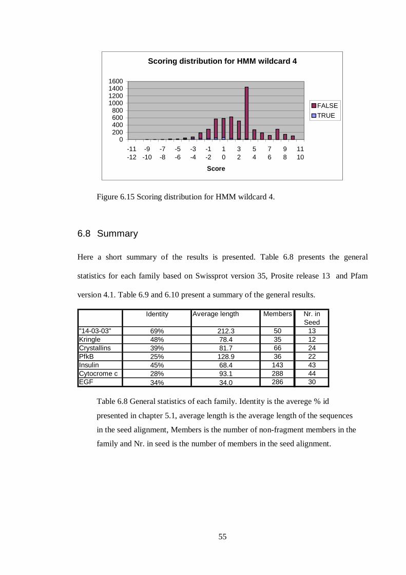
55


0200400600800

1000120014001600

-11-12

-9-10

-7-8

-5-6

-3-4

-1-2

10

32

54

76

98

1110

Score

FALSE

TRUE


6.8 Summary

Here a short summary of the results is presented. Table 6.8 presents the general

statistics for each family based on Swissprot version 35, Prosite release 13 and Pfam

version 4.1. Table 6.9 and 6.10 present a summary of the general results.

Average length Members Nr. inSeed

"14-03-03" 50 13Kringle 35 12Crystallins 66 24PfkB 36 22Insulin 143 43Cytocrome c 288 44EGF 286 30

45%28%

Identity

39%25%

34%

212.378.481.7128.968.493.134.0

69%48%

Table 6.8 General statistics of each family. Identity is the averege % id

presented in chapter 5.1, average length is the average length of the sequences

in the seed alignment, Members is the number of non-fragment members in the

family and Nr. in seed is the number of members in the seed alignment.

56

Sens Spec CC Sens Spec CC Sens Spec CC"14-03-03" 1.00 1.00 1.00 0.96 1.00 0.98 0.98 0.65 0.80Kringle 1.00 0.91 0.95 0.98 1.00 0.99 1.00 0.92 0.96Crystallins 1.00 0.22 0.47 0.95 1.00 0.98 1.00 0.89 0.94PfkB 0.61 0.48 0.54 0.81 1.00 0.90 1.00 0.86 0.93Insulin 0.99 0.99 0.99 0.97 0.97 0.97 0.97 0.98 0.98Cytocrome c 0.98 0.42 0.63 0.62 0.98 0.78 0.70 0.93 0.81EGF 0.73 0.80 0.74 0.77 0.71 0.74 0.97 0.40 0.62

PROSITE MAMA SAM1

Table 6.9 Summary of the general results for PROSITE, MAMA and SAM 1.

Sens Spec CC Sens Spec CC Sens Spec CC"14-03-03" 0.98 0.65 0.80 1.00 1.00 1.00 1.00 1.00 1.00Kringle 1.00 0.92 0.96 1.00 1.00 1.00 1.00 1.00 1.00Crystallins 0.98 0.94 0.96 1.00 1.00 1.00 1.00 1.00 1.00PfkB 0.89 0.91 0.90 0.97 1.00 0.99 0.93 1.00 0.96Insulin 0.99 0.98 0.98 0.99 1.00 1.00 0.99 1.00 1.00Cytocrome c 0.65 0.95 0.78 0.86 0.86 0.86 0.85 0.83 0.84EGF 0.98 0.35 0.58 0.11 0.63 0.26 0.10 0.59 0.24

SAM2 Best NS HybridBest Hybrid

Table 6.10 Summary of the general results for SA; 2, and the hybrid method.

Further discussion can be found in the next chapter.

57

7 Analysis

In this chapter the results presented in the previous chapter are analysed further. Each

family is discussed in a separate section, giving further interpretation of the results

presented in the previous chapter.

In order to explore the sensitivity versus specificity for each method graphs showing

different weightings are presented. Those can be used to compare the different strengths

and weaknesses of each method. The equation for calculating the strength is:

[ ] ( )[ ]SpecwSenswSt ∗−+∗= 1 Where 0.0 ≤ w ≤ 1.0

The graphs then show plots of St for w values in the range [0.0, …, 1.0] for each

method.

7.1 14-3-3

The 14-3-3 family is not hard to model, as can be seen by the fact that the simple

PROSITE pattern gives no false positives or false negatives. The MAMA pattern has 2

false negatives before generalisation and 12 after (see table 6.1). The increased

sensitivity comes at the cost of decreased specificity, but by using the probabilistic

models the specificity is again increased. The scoring distribution in Figure 6.1 shows

that there is a clear separation between the true and the false hits. In the PROSITE

documentation it is clamed that the family is well-conserved and therefore easy to

model. The PROSITE pattern is better than the pattern used for generalisation, but with

the hybrid method the model is improved to full sensitivity and specificity.

58

Hybrid PROSITEMAMA

HybridSAM 1 SAM 2

0 0.2 0.4 0.6 0.8 10

0.5

1

w

St

0 0.2 0.4 0.6 0.8 10

0.5

1

14-3-3

St

Figure 7.1 Sensitivity versus specificity weighting for the best hybrid

compared to the other methods.

As can be seen in Figure 7.1 the discrete methods do as well , or almost as, well as the

hybrid method while the HMM methods have much less specificity and about equal

sensitivity. Advantage of the hybrid over HMM is highest for low values of w, i.e. when

specificity is given higher importance.

The distribution analysis gives worse results than PROSITE and at best it gives 2 false

positives, that is rejecting 10 of the false positives picked up by the generalised pattern.

7.2 Kringle

The kringle family has 4 false positives using the PROSITE pattern and in the MAMA

pattern used for generalisation performs better with only one false negative. Using the

hybrid method improves the model even further, resulting in a better model than the one

59

devised with SAM as well as being better than the patterns in MAMA and PROSITE.

This shows an example where the hybrid method gives the “best of both worlds”,

making a better model than the probabilistic or discrete methods do when used

separately.

The experiment on this family also shows that the flanking model gives good results as

well as the internal one. This indicates that when the pattern is lacking internal

wildcards of the necessary size to model with probabilistic methods then the flanks can

be used to give probabilistic measures.

For both the internal wildcard and the flanking model the scoring distribution shows

that it is a clear separation between the true and the false hits for the generalised pattern.

The scoring distribution for the flanking model can even be seen as better than for the

internal wildcard as the gap is larger and the distribution of the true hits is such that the

number grows as the score get lower (see Figure 6.2 and 6.3).

In Figure 7.2 it can be seen that the hybrid method has a slightly better results than the

other methods. It is especially the middle area of the Figures that are of importance as

there the weighting of sensitivity and specificity are equal, giving an estimate of which

method has best of both. In the middle the hybrid method has the best results compared

to the other methods. Figure 7.2 also shows that for this family, the small advantage of

the hybrid method is relatively independent of the w value.

Here distribution analysis modelling does not improve the results for the generalised

pattern, since it fails to reject the single false positive picked up by the generalised

pattern.

60

Hybrid PROSITEMAMA

HybridSAM 1 SAM 2

0 0.2 0.4 0.6 0.8 10

0.5

1

Kringle

St

0 0.2 0.4 0.6 0.8 10

0.5

1

w

St



7.3 Crystallins

Here the results show the same as in the kringle family, i.e. that the hybrid method

generates better models than the other methods. The flanking model is however not as

good and this could indicate that even if the sequences in the family are longer than the

pattern, the sequence parts beyond the pattern have little to do with the family

characteristics (such as folding). This can also indicate that in the kringle family the

pattern could be extended into the direction covered by the flanking model as it proved

equally good as the internal wildcard. In other words there are indications that the flank

does have some influences on the general characteristics of the kringle family.

61

Looking at the scoring distribution for the internal wildcard (figure 6.4), it can be seen

that in most cases the separation is large, however there are two true hits that are very

far from the main group of the true hits. Still it is possible to identify a cut-off such that

the false hits of the generalised pattern are clearly separated from the true hits.

Hybrid PROSITEMAMA

HybridSAM 1 SAM 2

0 0.2 0.4 0.6 0.8 10

0.5

1

Crystallins

St

0 0.2 0.4 0.6 0.8 10

0.5

1

w

St



In Figure 7.3 it can be seen that PROSITE has by far the worst results, while the other

methods give results comparable to the hybrid method. The hybrid method is, however,

still better at intermediate w values.

The distribution analysis gives little (if any) improvement to the generalised pattern,

specificity is increased at the cost of decreased sensitivity. Compared to the original

MAMA pattern the results for the distribution analysis are bad.

62

7.4 PfkB

The generalised pattern for the PfkB family is large and has one very large wildcard.

The large wildcard does not give full sensitivity and specificity. However when the

scores for a seemingly bad wildcard, which has 9 false positives and 2 false negatives,

are added, then the specificity is increased at no cost in sensitivity. In other words a

seemingly too small wildcard that in itself does not give an adequately good model,

improve the results when added to a model that is based on a larger wildcard.

When looking at the scoring distribution (figure 6.5, 6.6, and 6.7) it can be seen that

even if it is possible to find a cut-off value that gives good results, the separation is not

so good for some sequences. For example in figure 6.7 there are both true and false hits

in the scoring range from 20 to 30 and also from 30 to 40. It is however possible to set

the cut-off so that the true and false hits in the 20 to 30 scoring range are separated

correctly. Then the single true hit in the scoring range 30 to 40 is the false negative seen

in table 6.4.

From Figure 7.4 it can be derived that the worst performance is that of PROSITE and

that the other pure discrete or probabilistic methods are quite similar with the best

hybrid, especially for intermediate w values.

Using distribution analysis for the wildcards instead of HMM does not give good

results, the sensitivity of the generalised pattern is lost at very little or no gain in

specificity.

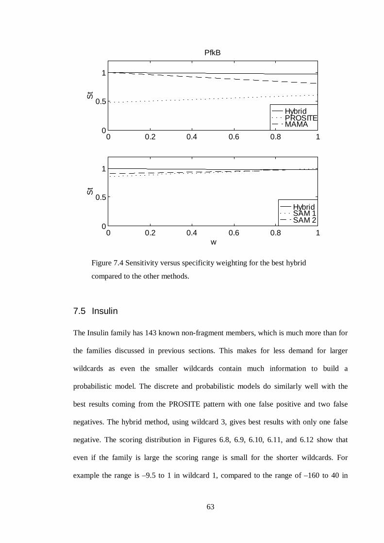
63

Hybrid PROSITEMAMA

HybridSAM 1 SAM 2

0 0.2 0.4 0.6 0.8 10

0.5

1

PfkB

St

0 0.2 0.4 0.6 0.8 10

0.5

1

w

St



7.5 Insulin

The Insulin family has 143 known non-fragment members, which is much more than for

the families discussed in previous sections. This makes for less demand for larger

wildcards as even the smaller wildcards contain much information to build a

probabilistic model. The discrete and probabilistic models do similarly well with the

best results coming from the PROSITE pattern with one false positive and two false

negatives. The hybrid method, using wildcard 3, gives best results with only one false

negative. The scoring distribution in Figures 6.8, 6.9, 6.10, 6.11, and 6.12 show that

even if the family is large the scoring range is small for the shorter wildcards. For

example the range is –9.5 to 1 in wildcard 1, compared to the range of –160 to 40 in

64

wildcard 3. This shows that while the smaller wildcards do not perform as well as the

larger wildcards even when the family is large as in this case, still in the Insulin family

they do as well as those of pure discrete or probabilistic modelling3.

Hybrid PROSITEMAMA

HybridSAM 1 SAM 2

0 0.2 0.4 0.6 0.8 10

0.5

1

Insulin

St

0 0.2 0.4 0.6 0.8 10

0.5

1

w

St



The weighting diagram in Figure 7.5 does not show clearly the differences between the

different methods, but if table 6.9 is examined it can be seen that the hybrid method is

performing slightly better. However all methods perform well on this family.

3 The biological databases, and especially those containing DNA and protein sequences, are growing at

an ever-increasing rate. With this growth the families are getting bigger and therefore pattern generation

is getting harder, the hybrid method can help the pattern modelling methods and databases to stay in the

game.

65

Using distribution analysis to model the wildcards of the hybrid gives worse results than

just using the generalised pattern, i.e. it introduces false negatives at no gain in

decreased number of false positives.

7.6 Cytochrome c

The difficulties with the cytochrome c family start with the pattern. It is hard to generate

any pattern that accepts all 288 non-fragment members of the family. The PROSITE

pattern gives good sensitivity at the cost of low specificity and the MAMA pattern gives

good specificity at the cost of low sensitivity. However, to generate a generalised

pattern that had no false negatives gives the generalisation method problems. The

method for generating patterns is however not the critical part of the hybrid method, and

any pattern generation method can be used to generate a pattern for generalisation. Here

a pattern generated from a ClustalW alignment was used for generalisation with

acceptable results. The pattern however accepts 1335 false positives when it has been

generalised to have no false negatives, so that there is an increased burden on the

probabilistic part. The probabilistic part has also problems as there is only one wildcard

large enough to be modelled with probabilistic methods. This wildcard has a very small

minimum length: only 3 amino acids. Such a small minimum size makes it hard to

model. The flanking model also has much length variation making it hard to model, but

still does better than the internal one.

66

Hybrid PROSITEMAMA

HybridSAM 1 SAM 2

0 0.2 0.4 0.6 0.8 10

0.5

1

Cytocrome C

St

0 0.2 0.4 0.6 0.8 10

0.5

1

w

St



It can be seen in Figure 7.6 that the hybrid method is not the best one in pure sensitivity

and specificity, but in the middle region, where the combination of both come in to

account then the hybrid method is better. It can be argued that this region, where

sensitivity and specificity are assigned approximately equal importance, is the most

important one.

Using distribution analysis instead of HMM to model the probabilistic parts gives bad

results here as in previous examples.

7.7 EGF-like domain

The EGF family is very hard to model, which is the reason it was selected for the

experiment. The discrete methods have about equal sensitivity and specificity, however

67

the number of false positives and negatives is between 60 and 92 (see table 6.7). The

HMM methods have much better sensitivity at the cost of low specificity. “The best of

both worlds” would then be to have the specificity of the discrete models and the

sensitivity of the probabilistic models. The problem is that the hybrid uses the discrete

part to get the sensitivity and the probabilistic part to get the specificity, and this causes

the hybrid to give “the worst of both worlds” instead. The EGF family is known to give

HMM methods problems, e.g. in the Pfam documentation (Accession number:

PF00008) it is clamed that “there is no clear separation between noise and signal”.

Looking at figure 6.14 it is clear that this is also the case with the HMM models for the

wildcard.

The fact that the generalised pattern has 4048 false positives contributes also to the bad

results of the hybrid method. Generating any kind of model for a family of such short

sequences (average length is 34 amino acids, see table 6.8) is hard, and generating a

model based on two different methods seem to be even harder.

The distribution analysis does not give any results, since all sequences are rejected,

giving all the 286 known non-fragment members as false negatives.

68

Hybrid PROSITEMAMA

HybridSAM 1 SAM 2

0 0.2 0.4 0.6 0.8 10

0.5

1

EGF

St

0 0.2 0.4 0.6 0.8 10

0.5

1

w

St



69

8 Discussion

8.1 Method

The pattern part of the method does the preliminary selection, accepting or rejecting

sequences depending on if they match the pattern or not. Also the pattern serves as an

anchor finding areas of the sequence that the probabilistic models (the wildcard models)

should be matched to. This makes the probabilistic parts of the method concentrate on

smaller areas of the sequence making matching faster as the search for the best scoring

match has fewer options that for example a HMM of the whole family that needs to be

aligned to the whole sequence. Focusing the matching of the probabilistic parts on a

predetermined sequence part, determined with the pattern, works to concentrate search

for the match on the correct area of the sequence.

8.1.1 Advantages and Disadvantages

Here some advantages and disadvantages of the method are presented.

The clearest disadvantage of the method as presented here is that the pattern

generalisation algorithm is not fully automated. Also the choice of which wildcards are

selected for probabilistic modelling is not based on any specific methodology, and can

be said to be ad hoc. Another disadvantage is that there are families such as the EGF

family that the method does not do well on. Also a disadvantage of the method is that it

is more complex compared to using pure discrete or probabilistic methods.

The clearest advantage is that the method has better results, compared to the other

methods, on all but one of the families used in the experiment. The one that the method

does worse on is known to be very hard to model with any method. Even the Cytocrome

c family is known to be very hard to model, and is often used in such experiments for

70

that reason. It does give the method some problems but still it performs slightly better

than the pure discrete or probabilistic methods used for comparison.

8.2 Thesis

The contribution of this thesis is that there are no other known work on a hybrid of

discrete and probabilistic methods for sequence family modelling. Here an approach is

described to do this combination, and the approach is compared to other methods, most

of which are established and widely used for modelling sequence families. The method

does well in most of the comparisons and the pros and cons of the method are described.

The disadvantages of this work are mainly the ad hoc parts of the method which need to

be explored further, for example the minimum length of a wildcard to be used for the

probabilistic part and the use of multiple alignment to generalise especially difficult

patterns.

8.3 Continued Work

The most important future work is the modelling of more sequence families to get more

detailed knowledge of what makes the method do badly in certain cases, as on the EGF

family.

The implementation and tuning of an algorithm for generalising the patterns is also an

important future work. This can be done starting on the algorithm described in this

work, but it will take much work to automate the whole process.

Generating guidelines and specific requirements for selecting which wildcards are used

in the probabilistic part is also future work that is of importance to generating a

modelling tool.

A final point in this work would be to build a database of hybrid models of all known

protein sequence families, and a tool for using that database to analyse newly

71

discovered protein sequences. The generation and maintenance of such a database

would be the final step in the work begun with this thesis.

72

9 Conclusion

This thesis presents a hybrid method for protein sequence modelling that combines

discrete patterns and probabilistic models based on HMMs. The hypothesis is in three

parts, which can be summarised as follows:

1. Such a method is valuable to use to model families of protein sequences.

2. Such a method improves the pattern generation methods that it is based on.

3. Such a method gives “the best of both worlds”, performing better than what pure

discrete and pure probabilistic methods do individually.

The results are promising, in 6 of the 7 protein families used in the comparison the

hybrid shows better results than the methods compared to. The family that the hybrid

method has problems modelling is known to be hard to model, and helps to identify the

weaknesses of the method. One weakness is that if the pattern only has wildcards with

low minimum length (e.g. 3 or 4 residues), then there is not enough information in the

wildcard to build a model. Also families of very short sequences are hard to model for

the same reason. For example the EGF family has average length of 34 residues, which

is not enough to build both discrete and probabilistic models on.

However, in all families except EGF the three parts of the hypothesis stand. This is to

say that if the family has long enough sequences to build a hybrid model then the

hypothesis is valid.

73

Acknowledgements

My thanks to my supervisor Björn Olsson, and co-supervisor Kim Laurio. The general

idea of combining patterns and HMMs is originated from them and also the MAMA

method, which this work uses to build on.

74

References

Attwod, T. K., Beck, M. E., Bleasby, A. J., Degtyarenko, K., Michie, A. D., Parry-

Smith, D. J., 1997. Novel developments with the PRINTS protein fingerprints database.

Nucleic Acids Research, 25(1):212-216.

Attwood, T. K., 1997a. Exploring the language of bioinformatics. In Oxford Dictionary

of Biochemistry and Molecular Biology, Ed Stanbury H., Oxford University Press, 715-

723.

Attwood,T. K. 1997a. Databases from universities – PRINTS, a research tool that has

grown into a resource. In Proceedings of Financing Biotechnology Databases,

Purmeren, The Netherlands, 29-30 May 1997.

Attwood, T. K. (1999). The PRINTS Fingerprint Database, THE PRINTS USER

GUIDE [online]. Available from: http://www.biochem.ucl.ac.uk/bsm/dbbrowser/

PRINTS/printsman.html [Accessed 22 June1999].

Bolsover, S. R., Hyams, J. S., Jones, S., Shephard, E. A., White, H. A. 1997. From

Genes to Cells. Wiley-Liss.

Bucher P., Bairoch A., 1994. A generalized profile syntax for biomolecular sequences

motifs and its function in automatic sequence interpretation. In ISMB-94; Proceedings

2nd International Conference on Intelligent Systems for Molecular Biology. Altman R.,

Brutlag D., Karp P., Lathrop R., Searls D., Eds., 53-61, AAAI Press.

Bucher, P. 1997. A generalised profile syntax for protein and nucleic acid sequence

motifs. [online]. Version 1.3 may 1997. Available from:

http://www.expasy.chuge/txt/prosuser.txt. [Accessed 10 mars 1999].

75

Blatch, G.L., Scholle R.R., Woods D.R. Gene 95:17-23. 1990

Burset, M. and Guigó, R. 1996 Evaluation of gene structure prediction programs.

Genomics, 34,353-367.

Dunker, A.K., Garner, E., Guilliot, S., Romero, P., Albrecht, K., Hart, J., Obradovic, Z.,

Kissinger, C., and Villafranca, J.E., 1998. Protein Disorder and the Evolution of

Molecular Recognition: Theory, Predictions and Observations. In Pacific Symposium on

Biocomputing. 3: 471-782.

Durbin, R., Eddy, S., Krogh, A., Mitchison, G. 1998. Biological sequence analysis.

Probabilistic models of proteins and nucleic acids. Cambridge University Press.

Eddy, S. R. 1998. Profile hidden Markov models, Bioinformatics review, 14(3): 755-

763.

Gracy, J., Argos, P. 1998. Automated protein sequence database classification. I.

Integration of compositional similarity search, local similarity search, and multiple

sequence alignment. In Bioinformatics, 14(2):164-173.

Henikoff, S., Henikoff, J.G., Alford W.J., & Pietrokovski, S. Automated construction

and graphical presentation of protein blocks from unaligned sequences, Gene-COMBIS,

Gene 163, GC 17-26.

Hughey, R., Krogh, A., Barrett, C., Grate, L. 1996. SAM Sequence Alignment and

Modeling Software System. Technical Report UCSC-CRL-95-7. University of

California. (January 1995. Updated 1996).

Hughey, R., Krogh, A. 1996. Hidden Markov models for sequence analysis: Extension

and analysis of the basic method, CABIOS. February 1996.

76

Jonassen, I., Collins, J. F., Higgins, D. 1995. Finding flexible patterns in unaligned

protein sequences. Protein Science 4(8):1587-1595.

Jonassen, I. 1996a. Scoring function for pattern discovery programs taking into account

sequence diversity. Technical Report 116, Dept. of Informatics, Univ. of Bergen.

Jonassen, I. 1996b. Methods for finding motifs in sets of related biosequences. Dt.

Scient. Thesis. Department of Informatics. University of Bergen, Norway.

Karplus, K. 1995. Evaluating regularizers for estimating distributions of amino acids. In

Proc. Of ISMB95. Eds. Rawlings, C. Clark, D. Altman, R., Hunter, L., Lengauer, T.,

Wodak, S. AAAI Press.

Krogh, A., Brown, M., Mian, I. S., Sjölander, K., Hausser, D. 1994. Hidden Markov

models in computational biology: Applications to protein modelling. Journal of

Molecular Biology, 235:1501-1531, February 1994.

Laurio, K. 1997. Finding remote protein homologs with hidden Markov models. MSc

dissertation Dep. Of Comp. Sc. University of Skovde. Sweden.

Lundh D., Kallberg Y., Persson B., Mandal A., Olsson B., Narayanan A. 1998.

ClustalW against HMM/SAM: round 1, CISM school-Workshop in Computational

Biology, Udine.

Nevill-Manning, C. G., Sethi, K. S., Wu, T. D., Brutlag, D. L. 1997. Enumerating and

Ranking Discrete Motifs. In Proc. ISMB5. 202.

Nevill-Manning, C.G., Wu, T.D., Brutlag, D.L. 1998. Highly Specific Protein

Sequence Motifs for Genome Analysis. In Proc. Natl. Acad. Sci USA 95, In Press.

77

Olsson B., Laurio K. 1998. Discovery of Diagnostic Patterns from Protein Sequence

Databases,: Proceedings of the Second European Symposium on Principles of

Knowledge Discovery and Data Mining (PKDD98), Eds. Quafafou, M., Zytkow, J.

Springer.

Olsson B. 1999. Using Evolutionary Algorithms in the Design of Protein Fingerprints",

In: GECCO-99: Proceedings of the Genetic and Evolutionary Computation Conference,

Eds. Banzhaf W. and Daida R.E. Morgan Kaufmann.

Prescot D. M., 1988. CELLS, Principles of molecular structure and function. Jones and

Bartlett Publisers, Boston.

Rabiner, L. R. 1989. A tutorial on hidden Markov models and selected applications in

speech recognition. Proc. IEEE, 77 (2), 257-286

Sander C. & Schneider R., 1991 Database of homology-derived protein structures.

Proteins, Structure, Function & Genetics, 9:56-68.

Searls, D.B. 1997. Linguistic approaches to biological sequences. CABIOS invited

review. Vol 13 (4) pp 333-344.

Sjölander, K., Karplus, K., Brown, M., Hughey, R., Krogh, A., Mian, I.S., Hausser, D.

1996. Diriclet mixtures: A method for improved detection of weak but significant

protein sequence homology. CARBIOS, 12(4):327-45.

Sonnhammer, E. L. L., Eddy, S. R., Durbin, R. 1997. Pfam: A comprehensive database

of protein domain families based on seed alignments. Proteins, 28:405-20.

78

Wu, L. F., Reizer, A., Reizer, J., Cai, B., Tomich, J. M., Saier, M.H. Jr. J. Bacteriol.

1991. Nucleotide sequence of the Rhodobacter capsulatus fruK gene, which encodes

fructose-1-phosphate kinase: Evidence for a kinase superfamily including both

phosphofructokinases of E. coli. J. Bacteriol., 173: 3117-3127.

Orchard, L.M.D. Kornberg, H.L. 1990, Proc. R. Soc. Lond. B, Biol. Sci. 242:87-90

Wu, T. D. and Brutlag, D. L. 1995. Motif Identification Using Conserved Properties and

Partitioning Techniques. Intelligent Systems for Molecular Biology-95. 402-4104.

4 The name on the paper is “Identification of Protein Motifs Using Conserved Amino Acid Properties and

Partition Techniques”.

Combining Probabilistic and Discrete Methods for Sequence - DiVA

Documents

Transcript of Combining Probabilistic and Discrete Methods for Sequence - DiVA