1

Combining EEG and eye movement recording in free viewing: pitfalls and possibilities

Andrey R. Nikolaev*, Radha Nila Meghanathan, Cees van Leeuwen

Laboratory for Perceptual Dynamics, Brain & Cognition Research Unit, KU Leuven -

University of Leuven, Leuven, Belgium

* Corresponding author

Laboratory for Perceptual Dynamics,

Brain & Cognition Research Unit,

KU Leuven - University of Leuven,

Tiensestraat 102, Box 3711,

3000 Leuven

Belgium

Tel +32 16 37 32 68

Fax +32 16 32 60 99

Andrey.Nikolaev@kuleuven.be

*REVISED Manuscript UNMARKEDClick here to view linked References

2

Abstract

Co-registration of EEG and eye movement has promise for investigating perceptual processes

in free viewing conditions, provided certain methodological challenges can be addressed.

Most of these arise from the self-paced character of eye movements in free viewing

conditions. Successive eye movements occur within short time intervals. Their evoked

activity is likely to distort the EEG signal during fixation. Due to the non-uniform distribution

of fixation durations, these distortions are systematic, survive across-trials averaging, and can

become a source of confounding. We illustrate this problem with effects of sequential eye

movements on the evoked potentials and time-frequency components of EEG and propose a

solution based on matching of eye movement characteristics between experimental

conditions. The proposal leads to a discussion of which eye movement characteristics are to

be matched, depending on the EEG activity of interest. We also compare segmentation of

EEG into saccade-related epochs relative to saccade and fixation onsets and discuss the

problem of baseline selection and its solution. Further recommendations are given for

implementing EEG-eye movement co-registration in free viewing conditions. By resolving

some of the methodological problems involved, we aim to facilitate the transition from the

traditional stimulus-response paradigm to the study of visual perception in more naturalistic

conditions.

Keywords: eye tracking, electroencephalography, unconstrained visual exploration, peri-

saccadic brain activity, eye-fixation related potentials, saccade-related EEG distortion

3

1. Introduction

For studying the visual system, two measures that offer excellent temporal resolution are eye

tracking and electroencephalography (EEG). The information they provide is complementary:

eye tracking can tell us where observers fixate their gaze, and thus where they get their

information from; EEG registers how the brain responds to this information. Eye tracking and

EEG together, therefore, offer a comprehensive record of the visual system.

The first attempts to study eye movement in combination with EEG were made in the early

1950ies (Evans, 1953; Gastaut, 1951). Research since then has mainly been focused on the

immediate consequences of eye movement on the EEG signal (Becker, Hoehne, Iwase, &

Kornhuber, 1973; Billings, 1989a; Boylan & Doig, 1989; Csibra, Johnson, & Tucker, 1997;

Kazai & Yagi, 1999; Kurtzberg & Vaughan, 1982; Moster & Goldberg, 1990; Riemslag, Van

der Heijde, Van Dongen, & Ottenhoff, 1988; Thickbroom, Knezevic, Carroll, & Mastaglia,

1991; Yagi, 1979). Correspondingly, measurement was restricted to activity evoked by single

eye movements, within the framework of the traditional stimulus-response paradigm.

More recently, a new generation of video-based eye trackers has widened the use of co-

registration of eye movements and EEG (Nikolaev, Pannasch, Ito, & Belopolsky, 2014). In

particular, co-registration is increasingly becoming popular in conditions involving continued

exploration, i.e., free viewing1. Because it can be used in naturalistic conditions, co-

registration provides an exciting new paradigm for studying attention (Fischer, Graupner,

Velichkovsky, & Pannasch, 2013), memory encoding (Nikolaev, Jurica, Nakatani, Plomp, &

van Leeuwen, 2013; Nikolaev, Nakatani, Plomp, Jurica, & van Leeuwen, 2011), visual search

1 Note, that in this paper we use “free viewing” as a shortening for any unconstrained eye movement behavior,

regardless of whether this behavior serves any perceptual task or goal. This is different from the narrow usage of

“free viewing” to describe visual exploration only, without specific task, as can sometimes be found in the

literature.

4

(Dias, Sajda, Dmochowski, & Parra, 2013; Kamienkowski, Ison, Quiroga, & Sigman, 2012;

Kaunitz et al., 2014; Körner et al., 2014), reading (Dimigen, Sommer, Hohlfeld, Jacobs, &

Kliegl, 2011; Hutzler et al., 2007), and responses to emotionally charged visual information

(Simola, Le Fevre, Torniainen, & Baccino, 2015; Simola, Torniainen, Moisala, Kivikangas, &

Krause, 2013), just to mention some domains of basic research in which this technique is

successfully being used. In applied research, for instance on brain-computer interfaces, eye

movements are used for navigation to a virtual target object, while real-time analysis of the

co-registered EEG is used to confirm object selection (Lee, Woo, Kim, Whang, & Park, 2010;

Zander, Gaertner, Kothe, & Vilimek, 2011). This paper is intended for researchers who are

aiming to contribute to any of these fields, as well as those who want to explore new fields of

research with co-registration techniques. Assuming some initial familiarity with either eye

tracking or EEG measurement within a stimulus-response paradigm, we will introduce co-

registration under free viewing conditions, with particular emphasis on what its pitfalls are

and how they could be avoided.

In making the step from the stimulus-response paradigm to free viewing, we need to consider

a crucial discrepancy. Traditionally, the EEG signal is segmented according to an external

event, usually the onset of the stimulus or the response. Such markers are not available in free

viewing. Instead, the eye movements themselves, in particular the saccades, serve as natural

markers for EEG segmentation. To enable their use, some issues have to be addressed

regarding analysis and interpretation of data. Most of these derive from the fact that eye

movements, unlike experimenter-controlled signals in the stimulus-response paradigm, are

self-paced and occur in quick succession. As a result, EEG responses evoked by sequential

saccades overlap (Dandekar, Privitera, Carney, & Klein, 2012; Dias et al., 2013; Dimigen et

al., 2011). This could distort or mask the effects of experimental conditions. Such distortions,

5

moreover, can easily be mistaken for effects of experimental manipulation. To give a

somewhat simplistic example, suppose we are interested in the effect of stimulus size on

visual information processing. Inspecting the larger stimulus, however, will require larger

saccades. The EEG may differ solely because of larger saccades rather than because of any

differences in information processing.

Confounding effects are not always that obvious. For this reason, co-registration should start

from an assessment of the liability to confounding of the design chosen. Ideally, eye

movements should in all possible respects be equivalent between relevant conditions. In

practice, more often the question arises: can we identify a limited set of eye movement

characteristics that carries a risk of confounding, and what is the best strategy for controlling

it? Which eye movement characteristics are to be controlled will depend on the particular task

and experimental goal. For choosing the appropriate strategy, it is important to know which

effects eye movements typically have on EEG and in which intervals these effects are

typically encountered. Here we will describe the variety of forms these effects can take. This

will motivate a solution based on matching eye movement characteristics between conditions.

We believe that, in offering solutions to the problems of co-registration in free-viewing

conditions, our paper will contribute to making it feasible for a wide scientific community.

1.1. The main peri-saccadic EEG activity

In simultaneous EEG-eye movement analysis, segmentation of EEG into epochs can either be

done relative to saccade or to fixation onset, each of which may allow us to capture different

aspects of visual processing. Intuitively, activity time-locked to fixation onset may reflect

those processes better, which affect perception at the current fixation; whereas, activity time-

locked to saccade onset may be better suited for revealing processes related to eye movement

6

planning and execution. Since either way the epochs comprise the eye fixation interval, their

averages are indistinctly called eye-fixation related potentials (EFRP)2. Thus, EFRP is a

hybrid construct, combining an exploration-driven, eye movement induced signal with a

stimulus-driven one, the potential evoked by the visual features at fixation. EFRPs during

both controlled and free eye movement behavior have been studied for several decades

(Billings, 1989b; Devillez, Guyader, & Guerin-Dugue, 2015; Dimigen et al., 2011; Fudali-

Czyz, Francuz, & Augustynowicz, 2014; Kazai & Yagi, 1999; Körner et al., 2014; Nikolaev

et al., 2011; Rama & Baccino, 2010; Thickbroom et al., 1991; Yagi, 1979).

Since EFRPs have such a venerable history, we will adopt its terminology for describing the

time-frequency EEG activity around a saccade. Accordingly, we will distinguish: the saccadic

spike activity, named after what is known as the saccadic spike potential and the lambda

activity, named after the lambda wave/potential. Another important focus will be on the

activity that precedes saccade initiation, i.e. presaccadic activity.

The saccadic spike potential (SP) is a sharp wave at the saccade onset. The SP is elicited even

in darkness (Riggs, Merton, & Morton, 1974) as it originates from contraction of extra-ocular

muscles during the execution of a saccade (reviewed in Keren, Yuval-Greenberg, & Deouell,

2010). In the frequency domain, the SP is manifested in a range between 20 and 90 Hz (Keren

et al., 2010). Consistent with its myogenic nature, the main factors affecting SP amplitude are

size (Boylan & Doig, 1989; Keren et al., 2010; Riemslag et al., 1988) and direction of the

saccade (Keren et al., 2010; Moster & Goldberg, 1990; Thickbroom & Mastaglia, 1986). Its

muscular origin makes the SP an unlikely focus of studies addressing the information

processing aspects of visual perception. Yet, the SP plays an important role in co-registration

2 It would be more exact to distinguish the potentials time-locked to the fixation and saccade onsets by calling

them “fixation-related potentials” (FRPs) and “saccade-related potentials” (SRPs), respectively (e.g., Dimigen et

al., 2011).

7

research. Its dependence on saccade size is instrumental in assessing the reliability of various

analytical steps, such as the correctness of EEG segmentation and the quality of oculomotor

artifact correction, as well as for detecting mismatches between experimental conditions.

Thus, the spike potential could be a valuable marker to ensure the adequacy of combined

processing of eye movement and EEG.

The lambda potential is a positive wave about 100 ms after fixation onset (Evans 1953)3.

There is common agreement that the lambda potential is a response of the visual cortex to

changes in the retinal image due to the saccade (Dimigen, Valsecchi, Sommer, & Kliegl,

2009; Gaarder, Krauskopf, Graf, Kropfl, & Armington, 1964; Kazai & Yagi, 1999, 2003;

Riemslag et al., 1988; Thickbroom et al., 1991). In point of fact, the lambda potential is not

evoked when saccades are made in darkness or on a homogenous display (Evans, 1953;

Fourment, Calvet, & Bancaud, 1976); moreover, the lambda amplitude depends on the

difference in luminance between starting and ending locations of the saccade (Ossandón,

Helo, Montefusco-Siegmund, & Maldonado, 2010). The association of the lambda potential

with early visual processing is confirmed by the similarity in cortical sources of the lambda

potential to those of the component P1 in event-related potentials (Kazai & Yagi, 2003). In

the frequency domain, the lambda activity is manifested in the upper-theta and alpha bands

(6–14 Hz) (Dimigen et al., 2009; Ossandón et al., 2010).

Presaccadic activity is described in EFRP research as a slow positive wave over parieto-

occipital brain areas, which starts around 300 ms before saccade onset. This wave has

3 In the 1970-80ies there has been a long discussion on whether the lambda potential is evoked by saccade or by

fixation onset. On the one hand, latency of the lambda potential is time-locked to fixation rather than saccade

onsets. This suggests that the lambda potential reflects processes initiated by fixation onset (Billings, 1989a;

Yagi, 1979). On the other hand, averaging relative to the saccade and fixation onsets revealed different lambda

subcomponents (Thickbroom et al., 1991), suggesting that the lambda potential may be a compound of activity

evoked by both saccade and fixation onsets (Kazai & Yagi, 1999; Thickbroom et al., 1991).

8

sometimes been called the antecedent potential (Becker et al., 1973; Csibra et al., 1997;

Kurtzberg & Vaughan, 1982; Moster & Goldberg, 1990; Parks & Corballis, 2008; Richards,

2003). It may co-occur with a positive wave over the frontal areas (Gutteling, van Ettinger-

Veenstra, Kenemans, & Neggers, 2010; Richards, 2000). Presaccadic activity may reflect

processes related to planning in the visual system, such as oculomotor preparation (Csibra et

al., 1997; Kurtzberg & Vaughan, 1982; Richards, 2003), selection and transfer of attention to

the next saccade target (Kovalenko & Busch, 2016; Krebs, Boehler, Zhang, Schoenfeld, &

Woldorff, 2012; Wauschkuhn et al., 1998), and the anticipatory shift of receptive fields before

the saccade (“trans-saccadic remapping”) (Parks & Corballis, 2008).

Since attention moves to the target of the next fixation before saccade onset (Hoffman &

Subramaniam, 1995), presaccadic activity might indicate reallocation of attention in free

viewing. This was, indeed, confirmed in studies operating with a fixation heat map. A fixation

heat map is a map of the stimulus display wherein the color scale represents the duration and

density of fixation. Thus, the color indicates how attractive a region is as a fixation target: the

warmer the color, the more attractive the region. When the eyes are moved from cool- to

warm-color regions, amplitude of presaccadic activity is larger than vice versa. The

presaccadic activity, thus, reflects attention deployed to the next fixation location (Nikolaev et

al., 2013). In a multiple target search task, the presaccadic amplitude is more negative for

distractors following than preceding the fixation on a target. These results suggest that

presaccadic activity reflects memory uptake of target information (Körner et al., 2014).

Moreover, presaccadic activity predicts the success of visual short-term memory encoding. At

the encoding stage of a free viewing change-detection task, in case change was correctly

detected, the presaccadic potential was proportional in amplitude to saccade size; in case of

detection failure the amplitude did not correspond to saccade size (Nikolaev et al., 2011). This

9

implies that change detection failure results from mismatch of saccade and attentional target

during visual exploration. Together, these studies illustrate that effects of presaccadic activity

can readily be interpreted in relation to visual attention and visual working memory. Since

presaccadic activity occurs in a time interval that is crucial for perceptual and cognitive

processes involved in saccade guidance, presaccadic activity may be particularly indicative of

these processes.

1.2. Eye movement artifacts

Eye movement artifacts are well-known from event-related potential (ERP) studies. In these

studies, in order to reduce the number of oculomotor artifacts it is usually sufficient to instruct

participants to keep their eyes fixated on a designated location (e.g., the fixation cross) and to

refrain from blinking during stimulus presentation4. Contaminated trials can then simply be

excluded. In case blink or eye movement artifacts remain frequent in the ERP data, correction

methods can be used, such as regression (Gratton, Coles, & Donchin, 1983), principal

component analysis in combination with dipole modeling (Lins, Picton, Berg, & Scherg,

1993), or independent component analysis (ICA) (Jung et al., 2000). The efficiency of ICA

has been proven in hundreds of ERP studies over the last decade, making this technique the

most popular one for removal of ocular artifacts. ICA is readily applicable to artifact removal

in free viewing conditions.

Because in free viewing, EEG segmentation is determined by saccades, eye movement

artifacts are anything but sporadic. The availability of eye tracking information in co-

registration is beneficial for ocular artifact detection and correction (Dimigen et al., 2011).

Using eye tracking data improves the efficiency of selecting those artifact-related intervals,

which are most affected by saccade preparation and execution (Keren et al., 2010; Plöchl, 4 In that case, participants are asked to blink only in certain intervals, the so called “blink breaks”.

10

Ossandón, & König, 2012). For example, Plöchl and colleagues (2012) proposed a procedure

in which the variance of eye movement-related independent components was compared

between saccade and fixation intervals defined by eye tracking. In this manner, the corneo-

retinal dipole and eyelid artifacts can be eliminated and the saccadic spike activity can be

significantly reduced. Yet, even with precise selection of artifact-related components, ocular

artifacts cannot be completely separated from neural processes (Plöchl et al., 2012), leaving

correction methods at risk of removing activity of interest along with the artifacts.

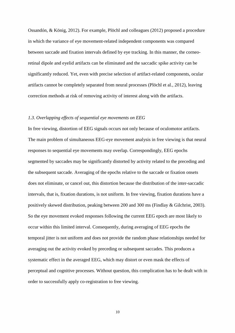
1.3. Overlapping effects of sequential eye movements on EEG

In free viewing, distortion of EEG signals occurs not only because of oculomotor artifacts.

The main problem of simultaneous EEG-eye movement analysis in free viewing is that neural

responses to sequential eye movements may overlap. Correspondingly, EEG epochs

segmented by saccades may be significantly distorted by activity related to the preceding and

the subsequent saccade. Averaging of the epochs relative to the saccade or fixation onsets

does not eliminate, or cancel out, this distortion because the distribution of the inter-saccadic

intervals, that is, fixation durations, is not uniform. In free viewing, fixation durations have a

positively skewed distribution, peaking between 200 and 300 ms (Findlay & Gilchrist, 2003).

So the eye movement evoked responses following the current EEG epoch are most likely to

occur within this limited interval. Consequently, during averaging of EEG epochs the

temporal jitter is not uniform and does not provide the random phase relationships needed for

averaging out the activity evoked by preceding or subsequent saccades. This produces a

systematic effect in the averaged EEG, which may distort or even mask the effects of

perceptual and cognitive processes. Without question, this complication has to be dealt with in

order to successfully apply co-registration to free viewing.

11

The problem of overlapping EEG activity due to eye movement was raised in various

domains of study, such as viewing natural scenes (Devillez et al., 2015), visual search

(Dandekar, Privitera, et al., 2012; Dias et al., 2013), and reading (Dimigen et al., 2011;

Hutzler et al., 2007). Even though these domains have their idiosyncrasies in saccade size,

fixation duration, or predominant saccade direction (in particular in reading), the general

shape of the fixation duration distribution is the same, and thus the problem of overlapping

EEG activity is common between them. The problem is nicely illustrated in the reading study

by Dimigen and colleagues (2011): their figure 2B shows how the temporal distribution of

preceding and subsequent fixation onsets affects EEG before and after the current saccade.

Here, with the saccadic spike activity removed by artifact rejection, the activity that

contributes most to the problem of overlap appears to be the lambda responses. Later, we will

demonstrate the dominant role of lambda activity in overlapping effects.

Attempts have been made to statistically eliminate distortions due to overlapping EEG

responses through linear regression (Dandekar, Privitera, et al., 2012; Dias et al., 2013). Using

the general linear model Dandekar and colleagues (2012) built and zeroed out eye movement

regressors for five saccade sizes in the interval +/- 492 ms relative to the saccade onset, an

interval that included a sequence of approximately three saccades. To remove activity from

the interval +/- 3 s relative to the saccade onset, Dias and colleagues (2013) used a method

called subspace subtraction. This method is similar to the standard regression approach for

ocular artifact correction but considers all EEG and eye movement channels in constructing

an optimal estimate of the to-be-removed activity. In contrast to ICA, which identifies activity

“blindly” (i.e., without the experimenter’s selective intervention) based on a statistical

independence assumption, Dias and colleagues (2013) explicitly specified the information

12

needed to build the regressors: the activity evoked by vertical and horizontal saccades and the

saccadic spike potential.

Not only are these procedures mathematically complex and difficult to implement but, more

importantly, the linear model may not consider the full variety of factors that contribute to

overlapping EEG responses in free viewing. For example, Dandekar and colleagues (2012),

whose model considered only saccade size, cautioned that it cannot take into account other

factors known to contribute to the lambda response, such as saccade direction or change in

luminance between images at saccade onset and offset.

In addition, the linear model is insensitive to the nonlinearity of overlapping EEG responses.

Nonlinearity could be accounted for by generalized additive mixed modelling (GAMM),

which considers the EEG signal as an additive structure of nonlinear smoothing functions

(Tremblay & Newman, 2015; Wood, 2006). Specifically, GAMM combines a parametric part

with a non-parametric part, which provides nonlinear smoothing functions for modeling

surfaces of two or more numerical predictors. The use of nonlinear regression techniques in

modeling eye movement evoked EEG activity is currently in the forefront of co-registration

research.

Problems have been raised with the construct validity of regression-corrected factors (Miller

& Chapman, 2001): regression involves a predictor variable (the covariate) and an

independent variable (the treatment). However, “when the covariate and the treatment are not

independent, the regression adjustment may obscure part of the treatment effect or may

produce spurious treatment effects” (p. 90, Wildt & Ahtola, 1978). Applying regression in

oculomotor behavior runs the risk of violating the assumption of independence because of

13

sequential dependencies between eye movements. Such dependencies are abundant. For

instance, in viewing natural scenes, large saccades have a tendency to be preceded by small

saccades; long fixations tend to be followed by long fixations (Tatler & Vincent, 2008). Also

trends and long-range dependencies have been reported in eye movements; as an example of

the first, extended visual exploration is characterized by decreasing saccade sizes and

increasing fixation durations (Unema, Pannasch, Joos, & Velichkovsky, 2005); as an example

of the second, the differences in distance and eye position across fixations show the signature

1/f noise, characteristic of memory operating across eye movements (Aks, Zelinsky, & Sprott,

2002). All these dependencies call for caution in applying statistical regression methods to

eye movement series.

To avoid potential misuse of statistical regression methods, Miller & Chapman (2001)

proposed the solution of matched sampling techniques. In the present context, matching

would offer a conservative alternative to regression-based methods. It involves comparing

between experimental conditions only those eye movements that are similar in size, direction,

and duration. Using this technique instead of regression is the method we will advocate here.

Matching of eye movement characteristics has previously been used in free viewing studies

(Devillez et al., 2015; Dias et al., 2013; Dimigen et al., 2011; Fischer et al., 2013;

Kamienkowski et al., 2012). Dias and colleagues (2013), however, did this in addition to

using their subspace subtraction technique to remove saccade-related distortion of EEG. We

argue that removing distortion does more harm than good. In our view, since distortion cannot

be reliably separated from the EEG signal of interest, it can better be left in the signal. After

matching eye movements any saccade-related distortions will be balanced across conditions.

1.4. The scope of the current paper

14

We will start our survey with a demonstration of the main peri-saccadic EEG activities in two

datasets (3.2). We will consider two ways of segmenting EEG: relative to either saccade or

fixation onsets (3.3). By comparing the saccade-locked and fixation-locked activity at

different EEG frequencies we will show which way of segmenting brain activity of interest is

preferable for obtaining the most prominent signal. The distortion of EEG waveforms by eye

movements also raises the problem of how to determine a proper interval for baseline

correction (3.4). We will consider several possibilities for selection of the baseline interval.

We will show how overlapping EEG signals may bias baseline correction and how this

problem could be addressed.

Next, we will consider to what extent different eye movement characteristics pose a risk of

confounding the EEG signal in free viewing conditions (3.5). We will consider six eye

movement characteristics: preceding and current saccade size5, saccade direction, and

duration of the fixations which precede and immediately follow the current saccade. We will

demonstrate where and when different eye movement characteristics are at risk of

confounding effects on the peri-saccadic EEG.

Even for single eye movements, their characteristics may not be independent of each other.

One example we will encounter in this study is the dependency between saccade size and

direction. Since saccade sizes tend to be smaller in upward than in other directions (3.5.4),

when we observe effects of saccade direction on EEG, the effect may occur indirectly,

because of a saccade size difference. More important for free viewing conditions are

interdependencies between sequential eye movement characteristics. These may vary,

according to the visual task (Tatler & Vincent, 2008).We will show how, for example,

5 In the simultaneous analysis of EEG and eye movements we prefer to refrain from using “saccade amplitude”

even though it is a common term in the eye movement literature. We reserve “amplitude” for EEG measures,

thereby avoiding confusion in the description of EEG and eye movements.

15

interdependency between current saccade size and preceding fixation duration may influence

the presaccadic EEG (3.5.3.1).

We will propose a solution to the problem of how to control for overlapping eye movement

effects (3.6). For reliable estimation of the saccade-related EEG it is crucial to match the

relevant eye movement characteristics across experimental conditions. We will describe a

procedure for matching based on the concept of Mahalanobis distance (Dias et al., 2013) and

discuss which eye movement characteristics have to be matched to analyze different peri-

saccadic activities.

To provide a broad picture of overlapping EEG activity during sequential eye movements we

will use the potentials time-locked to the saccade and fixation onsets as well as the time-

frequency data in the range from 5 to 45 Hz. This range is commonly studied in perceptual

and cognitive research. In the time-frequency domain, we will consider EEG amplitude

(power) as well as inter-trial coherence (ITC). ITC indicates synchronization of EEG signals

across trials in relation to a phase-locking event. ITC measures only the phase relationship

and does not depend on signal amplitude. We will compare the time course of saccade-related

changes in terms of power and ITC, and test the effect of the saccade and fixation onset, as

phase-locking events, on ITC values.

We will analyze saccade-related epochs corresponding to fixations longer than 200-300 ms

(2.5), in order to consider EEG activity uninterrupted by subsequent saccades. This will allow

reliable evaluation of the evoked components which correspond to the early components of

the ERP. Saccade-related components are commonly viewed as similar to the classical ERP

components elicited when stimuli are presented at fixation. Several studies demonstrated this

16

similarity for the early event-related components P1 and N1 (Belopolsky, Kramer, &

Theeuwes, 2008; Graupner, Velichkovsky, Pannasch, & Marx, 2007; Kazai & Yagi, 2003;

Ossandón et al., 2010; Rama & Baccino, 2010) as well as the late “cognitive” components

such as P300 (Brouwer, Reuderink, Vincent, van Gerven, & van Erp, 2013; Dandekar, Ding,

Privitera, Carney, & Klein, 2012; Kamienkowski et al., 2012; but see Dias et al., 2013 for an

opposite conclusion) and N400 (Dimigen et al., 2011). In free viewing, the latencies of the

early components most likely lie within the duration of a single fixation, whereas the latencies

of the late components may only appear after two or even three subsequent saccades. This

makes the late components more vulnerable to the issue of overlapping effects than the early

ones. In this context it is noteworthy that similarity of the event-related and saccade-related

P300 was shown in experiments where either eye movement behavior was controlled

(Brouwer et al., 2013; Dandekar, Ding, et al., 2012) or very long fixations in free viewing

were selected (Kamienkowski et al., 2012). However, typically, the study of the late

components in free viewing is based on the assumption that the perceptual or cognitive

processes reflected in these components are not affected by the processes that occur at the

onsets of the intervening saccades. There is no way to confirm that this assumption is sound.

But even if so, the intervening saccades produce overlapping EEG activity which should be

discounted. Matching eye movement characteristics, therefore, is a crucial step for analyzing

not only early but also late components. Specifically, when fixation durations are equal,

distortions of the current saccade-related activity by the subsequent saccade onsets will be

localized in the same interval for the experimental conditions during averaging. Then these

distortions can easily be eliminated by matching for characteristics of subsequent saccades

and computing the differential activity between the conditions.

2. Methods

17

We used two datasets of which the perceptual or cognitive implications were, or will be

published elsewhere. Here, they served only to illustrate the methodological issues that

distinguish a co-registration study from EEG or eye tracking experiments.

Change Blindness (CB) dataset

This dataset was previously used for a study on the perceptual and cognitive processes

associated with change blindness (Nikolaev et al., 2013; Nikolaev et al., 2011). Details about

the experimental design and procedure could be found in these publications. From the

recordings made during the task, here we used the data at the encoding stage. This is when

participants freely moved their eyes, looking at and memorizing a photograph of a natural

scene (Fig. 1A). In the photograph shown next, a change to the scene was made, which

participants were instructed to detect.

Visual Search (VS) dataset

This dataset was obtained for a study of information encoding in visual short-term memory. In

a combined visual search-change detection task, participants, first, had to find between 3 and

5 targets among distractors and then, in a subsequent test display, determine whether one of

the targets had its orientation changed. Analyses of fixation duration and pupil size as

indicators of memory load were published recently (Meghanathan, van Leeuwen, & Nikolaev,

2015); analysis of EEG related to experimental conditions is currently in progress. Here we

used EEG-eye movement data from the search display only, which was being inspected prior

to the change detection test display (Fig. 1B).

In neither of the datasets was there any restriction on viewing behavior, other than the total

time. Both tasks guaranteed that participants had an interest in visually exploring and

18

memorizing the display. Thus, these data are suitable for demonstrating the intricate effects of

eye movements on EEG. The stimulus displays, however, were quite different in character

between the two experiments. This led to different patterns of eye movement and EEG.

Moreover, differences in EEG recording systems between the two experiments led to

differences in EEG analysis. These will be detailed in later sections of this paper; here we

indicate the main differences, which may show that to a large degree the datasets were

complementary.

Saccade size and fixation duration distributions differed between the two datasets. The

proportion of small saccades was larger (Fig. 2A) and fixation durations were longer in the

CB than in the VS dataset (Fig. 2B). These differences most likely were due to the nature of

the displays, of which the contents had to be memorized. The CB dataset was obtained with

color photographs of natural scenes (Fig. 1A), whereas grey fields with relatively small

encircled letters were used for the VS dataset (Fig. 1B). The former thus contained a larger

amount of high spatial frequencies and a larger range of luminance differences. This

necessitated more scrutinizing eye movements: short saccades and long fixations. Therefore,

in the CB dataset the minimal fixation duration (and corresponding saccade-related epoch) for

inclusion in the analysis was 300 ms, whereas in the VS dataset it was 200 ms (see 2.5 for

details). The difference in the displays affected the lambda activity: it was 2-3 times higher in

the CB than in the VS dataset, as we will demonstrate below. This most likely occurred

because of the larger luminance difference between starting and ending locations of saccades

on color photos than on grey displays (Ossandón et al., 2010). Another difference between the

datasets was in the EEG recording system: for the CB dataset the EEG was recorded from 15

electrodes, whereas for the VS dataset EEG was recorded from 256 electrodes with a montage

19

that included peri-ocular channels. This enabled the use of electrooculogram (EOG) in an

ocular artifact correction procedure and application of an average reference.

The sections below and the Results section, unless otherwise stated, will describe the CB

dataset. The most important differences with the VS dataset will be discussed wherever they

arise. Detailed Methods for the VS dataset are described in the Supplementary Materials.

2.1. Participants

19 participants (five male) with normal or corrected-to normal vision took part in the CB

experiment. Their median age was 20 (range 19-24). All participants gave written informed

consent. The study was approved by the Research Ethics Committee of RIKEN Brain Science

Institute (Wako-shi, Japan) where the study was conducted. As we will describe below, here

we report the data from 15 participants whose numbers of epochs were sufficient for EEG

analysis.

2.2. Stimuli and procedure

48 pairs of color photographs were used as stimuli (Fig. 1A). All were real-world scenes from

Rensink et al. (1997). The photographs were pairwise identical, apart from a single detail.

This could be the color, position, or presence/absence of an object anywhere in the scene. The

images were presented on a 21-inch monitor placed at 85 cm from the participant and had a

size of 28° × 22° (width × height). During a trial, the first image of a pair was presented for

20 s. Participants were asked to explore and memorize the image. Then, after a 1-s mask, the

second image was presented. Participants were asked to find and indicate the change by

clicking a mouse button after placing the cursor on the change region. The second image

remained on the screen until response but no longer than 20 s. Feedback was given

20

immediately after the response by showing the second image again, with a red ellipse

encircling the changed region.

2.3. Eye movement recording

Eye movements were recorded with the EyeLink 1000 eye tracking system (SR Research

Ltd., Ontario, Canada). The CB experiment used the tower version, which has a chin and

forehead rest to stabilize the participant’s head. This allows obtaining higher precision of eye

positions during visual exploration than the desktop version of the eye tracker. The forehead

rest, however, makes it unfeasible to place electrodes for recording an electrooculogram. The

VS experiment used the desktop version of the eye tracker and a chinrest, which does not

impose any restrictions on placing electrodes around eyes.

Eye tracking was performed with a sampling rate of 500 Hz. We tracked the right eye only.

For calibration we used nine points falling in the center, four corners, and the mid-points of

the four sides of the screen. The difference between calibration and validation measurement

was kept below 1.5°.

2.4. EEG recording

The CB experiment used a Nihon Kohden MEG-6116 amplifier to record EEG with 0.5 Hz

high-pass and 100 Hz low-pass online filters and with a 50 Hz notch filter. The sampling rate

was 500 Hz. 15 electrodes (F3, F4, C3, C4, P3, P4, O1, O2, T3, T4, T5, T6, Fz, Cz, Pz) were

placed according to the international 10-20 system using an ECI electrode cap (Electro-Cap

International Inc., Eaton, USA). The ground electrode was FCz. The reference was the linked

mastoids.

21

In the VS experiment, EEG was recorded using a 256-channel Electrical Geodesic System

(Electrical Geodesics Inc., Eugene, OR). The electrode montage included channels for

recording vertical and horizontal EOGs. During recording the channels were referenced to the

vertex electrode (Cz), but in the analysis they were re-referenced to an average reference.

The choice of reference electrode determines the shape of EEG waveforms at each electrode,

but not the topographical distribution of EEG amplitude on the scalp surface. Most co-

registration studies of free viewing behavior use either a mastoid reference (Devillez et al.,

2015; Fischer et al., 2013; Graupner et al., 2007; Körner et al., 2014; Ossandón et al., 2010;

Rama & Baccino, 2010; Simola et al., 2015) or an average reference (Dandekar, Privitera, et

al., 2012; Dimigen et al., 2009; Kamienkowski et al., 2012). We used a mastoid reference in

the analysis of CB dataset because the limited number of electrodes did not allow us to

convert the data to average reference reliably (Dien, 1998) and an average reference in the

analysis of VS dataset, which was recorded from 256 electrodes.

Synchronization of the eye movement and EEG recordings was achieved as follows. In the

CB experiment, the horizontal eye movement coordinate was recorded as an additional

channel (the EyeLink channel) along with the regular EEG channels via analog connection

between the EyeLink system and the EEG amplifier. A blink-free segment with a length of

several seconds was selected in each trial. The lag of maximum correlation was found

between the EyeLink channel and the X coordinate time-series from the EyeLink data using

normalized cross-correlation (the correlation coefficient was always above 0.98). Then the

time stamps of the saccade onsets and offsets were adjusted for this lag and incorporated into

the EEG file (see for details Nikolaev et al., 2013). In the VS experiment, a TTL pulse was

22

sent at the beginning of each trial from the stimulus presentation computer via the parallel

port to both eye movement and EEG recording systems.

2.5. Setting limits on eye movement characteristics

Let the “current saccade” be the one on which the given analyses are centered. Relative to its

onset or offset (i.e., fixation onset), we considered the preceding fixation and saccade, as well

as the subsequent fixation, as schematically depicted above the relevant figures in the Results

section.

For eye movement data to be admitted to the analysis, we imposed the following restrictions.

The duration of the current saccade had to be smaller than 80 ms6. This restriction excluded

less than 0.1% of saccades. A saccade was also excluded if a blink occurred within -300 to

300 ms relative to saccade onset (or fixation onset depending on the type of segmentation, as

described in “Saccade vs. fixation onset” below). To discount the stimulus onset-related

potential, which may last up to 700 ms after stimulus onset (Dimigen et al., 2011), we

discarded the first fixation after image onset. Across participants the first fixation had a mean

duration of 1473 ms7 (SD = 451, range - 540-2115 ms). Discarding it, therefore, mostly

excluded the activity related to stimulus onset. For fixation duration we set a lower limit at

300 ms and an upper limit at 2000 ms. Whether these limits were imposed on the preceding or

subsequent fixation depended on the type of analysis, as specified in Table 1. The limits

6 As a measure of saccade size we used its duration rather than its length in degrees of visual angle because this

makes it easier to understand dependencies between latencies of EEG activities around a saccade. Saccade

duration and length are linearly related in a range from 1 to 50 degrees (Leigh & Zee 2006). Within this range,

saccade duration can be calculated from saccade length as follows: D = 2.2*L + 21, where D is the saccade

duration in ms, and L is the saccade length in degrees (Carpenter, 1988). This formula should serve for most

saccades in free picture viewing, which are overwhelmingly within a 2-4 degrees range (Findlay & Gilchrist

2003). 7 The unusually long duration of the first fixation probably occurred because the trial onset was relatively

unexpected for participants since each trial was started by the experimenter, only after the participant maintained

stable fixation over a central cross.

23

removed 59.6% of fixations and increased the mode of fixation duration from 214 to 306 ms

and the mean from 307 to 440 ms.

Table 1. Limits on fixation duration for different analyses.

Used in the analyses of Time-locking event

Preceding fixation duration, ms

Subsequent fixation duration, ms

Current saccade size and direction, preceding saccade size, preceding fixation duration, Saccade vs. fixation onset

Saccade onset

300 < pFD < 2000 No limit

Saccade vs. fixation onset Fixation onset

300 < pFD < 2000 No limit

Subsequent fixation duration Fixation onset

No limit 300 < sFD < 2000

Note. “pFD” indicates preceding Fixation Duration; “sFD” indicates subsequent Fixation Duration.

After removing fixations shorter than 300 ms we evaluated the number of intervals which

could be used as EEG epochs for each participant. Across all 48 trials there were on average

989 (SD=204, range 543-1343) epochs per participant. As we will describe below, we will

typically sort the EEG data into three bins with equal number of saccade-related epochs. To

obtain robust EEG estimation, we arbitrarily set the minimal number of epochs per bin to 300,

i.e., 900 in total per participant. We excluded four participants who did not reach this criterion

and analyzed the EEG-eye movement data from the remaining 15 participants.

2.6. Artifact removal

We analyzed EEG using Brain Vision Analyzer software (Brain Products GmbH, Gilching,

Germany). From the 15 recorded channels, we excluded two temporal channels (T3 and T4)

because of artifacts resulting from muscle activity. To remove ocular artifacts from EEG we

used ICA (Jung et al., 2000). Ocular artifact correction with ICA benefits from using EOG

recording, although it is also possible without EOG (Ma, Bayram, Tao, & Svetnik, 2011;

Romero, Mananas, & Barbanoj, 2008), as we will discuss in 4.4. EOG was available in the

24

VS but not in the CB dataset. Consequently, ocular artifact correction of VS dataset involved

correlation of ICA components with EOG (see Supplementary Materials), whereas from the

CB dataset we subjected 13 regular EEG channels to ICA for artifact correction.

At the first stage, ICA involves selection of a training dataset for computing the unmixing

matrix. Following the general rule that for ICA, the more data the better (Onton, Westerfield,

Townsend, & Makeig, 2006), we selected as training dataset a 400-s interval after skipping

the initial 3 minutes of the experiment. The dataset included several trials of the change

detection task. Among the ICA components that were obtained, we identified those which

picked up eye movement artifacts as was evident from their time course: these components

reflected the blinks and saccades in the EyeLink channel. These components typically had a

maximum at the frontal sites, with a characteristic asymmetrical topography corresponding to

saccade direction. Blink-related components were identified by their symmetrical maximum

at the frontal electrodes. After removing these components the whole EEG signal throughout

the session was reconstructed, which led, as expected, mainly to changes in the activity at the

frontal sites.

We removed other artifacts, due to large body movements, face/neck muscle activity, poor

electrode contact, etc., in the same manner as in ERP studies (Luck, 2005). To this aim, we

divided EEG into epochs from -1300 to +1300 ms relative to saccade or fixation onset. At this

stage of the analysis, such a long epoch duration was needed to avoid the marginal effects of

wavelet transformation, considering that our lowest frequency of interest was 5 Hz (see 2.7).

The artifacts were assessed, however, in the interval from -300 to 300 ms around saccade or

fixation onset. We rejected EEG epochs if the absolute voltage difference exceeded 50 µV

between two neighboring sampling points (as a threshold for a sudden voltage jump) and if

25

the amplitude exceeded +100 or -100 µV within an epoch (as a threshold for a slow drift).

Afterwards the mean number of epochs per bin was 332 (SD= 46; range 272-426) for

segmentation relative to saccade onset and 340 (SD= 44; range 283-429) for segmentation

relative to fixation onset8.

2.7. EEG analysis

The EEG data were analyzed only from the 20 s presentations of the first display, when

participants visually explored a photograph of a natural scene in order to memorize it.

We estimated the time-frequency structure of the EEG epochs using two-cycle Morlet

complex wavelets for 10 logarithmically-spaced center frequencies in the range from 5 to 45

Hz. Having a small number of wavelet cycles permits estimating EEG power and phase in

short time windows, albeit at the expense of frequency resolution (Alexander, Trengove,

Wright, Boord, & Gordon, 2006). The wavelet duration was 127 ms at 5 Hz and 14 ms at 45

Hz. The wavelets were normalized to have unit scale power to sample rate. After wavelet

transformation, the epoch duration was reduced to -300+300 ms relative to a segmentation

event. We extracted absolute power and phase. For the power we computed the natural

logarithm to approximate the normal distribution. In the CB dataset only, the phase was used

for computing inter-trial coherence (ITC) (Delorme & Makeig, 2004), aka the phase-locking

factor (Tallon-Baudry, Bertrand, Delpuech, & Pernier, 1996). ITC allowed us to evaluate

phase-locking of EEG signals to saccade and fixation onsets across EEG epochs. ITC was

calculated as proposed by Delorme and Makeig (2004):

8 The numbers differ slightly because the 600-ms epoch interval was shifted by the duration of the intervening

saccade (up to 80 ms) and artifacts near the edges of an epoch may appear within an epoch in one way of

segmentation but not in another.

26

where n indicates the number of trials, Fk (f, t) is the Fourier component of trial k at

frequency f and time t, estimated by Morlet wavelets. ITC values vary between 0 and 1, where

0 indicates no phase-locking and 1 indicates perfect phase-locking.

For analysis of the saccade-related potentials the EEG signal was filtered with a Butterworth

zero-phase filter with a high cut-off frequency of 45 Hz, 12 dB/oct. EEG was segmented into

epochs from -300 to +300 ms relative to the segmentation event. The epochs were averaged

relative to the saccade or fixation onsets. The averaged potentials, as well as the power and

ITC curves, were baseline corrected by subtracting a mean in the interval -300-250 ms before

the saccade or fixation onsets, unless otherwise stated.

To measure EEG power for an interval at a given frequency we extracted the mean values

over the interval. To measure the saccadic spike and lambda potentials we extracted peak-to-

peak amplitudes. For the saccadic spike potential the peak-to-peak amplitude was the

difference between positive and negative peak values. For the lambda potential the peak-to-

peak amplitude was the difference between the peak value of the lambda potential and the

preceding negative peak of the saccadic spike potential. The peak-to-peak amplitude measure

has the advantage that it is baseline independent. As we will discuss below (3.4), this is

important because baseline selection is complicated in co-registration analysis.

For statistical analysis, unless otherwise stated, we used pointwise t-tests and repeated-

measures ANOVA with the Huynh-Feldt correction of p-values associated with two and more

degrees of freedom, in order to compensate for violation of sphericity. The obtained p-values

were corrected for multiple comparisons using false discovery rate (FDR) (the version

27

proposed by Storey (2002) and implemented in the qvalue package for R). For post-hoc

comparison we used the Tukey HSD test.

3. Results

3.1. Eye movements

Saccade duration had a bimodal distribution for both datasets (Fig. 2A), with a mode of 22 ms

for the CB dataset and 24 ms for the VS dataset. The CB dataset had a larger number of small

(shorter than 20 ms) saccades than the VS dataset. This most likely occurred because of the

properties of the displays: since we used photos of natural scenes in the CB experiment versus

homogenous displays with sparsely placed letters in the VS experiment, the former contained

larger amount of high spatial frequencies than the latter.

Fixation durations were considerably longer in the CB than in the VS dataset (Fig. 2B): a

mode of 214 vs. 164 ms and a mean of 307 vs. 197 ms. This is also a most likely consequence

of the display difference because scrutiny of photos of natural scenes with a larger range of

luminance differences requires longer fixations than search for sparse letters on a

homogenous background.

We did not observe a substantial difference in saccade directions between the two datasets

(Fig. 2C). Both showed a prevalence of horizontal over vertical saccade directions, as is

typical for free viewing behavior (Tatler & Vincent, 2008).

3.2. EEG activity around a saccade

28

The grand averages of the saccade-related potentials, EEG power, and ITC from the CB

dataset are shown in Fig. 3. Those from the VS dataset are shown in Fig. 4. EEG power

increased at the latency of the saccadic spike potential (around the saccade onset); most

prominently at frequencies from 17 Hz and higher (Fig. 3A, 4B, E). The saccadic spike

activity may propagate to higher EEG frequencies, up to 90 Hz (Keren et al. 2010), which,

however, are out of the scope of our current analysis. ITC went up along with the power

increase (Fig. 3B). Saccadic spike amplitude and power were more prominent when time-

locked to the saccade (Fig. 4B) rather than to the fixation (Fig. 4E) onset. The saccadic spike

potential in the CB dataset (which used a mastoid reference) showed a biphasic wave, which

had the same polarity across all electrodes (Fig. 3A), similarly to the data with a nose

reference reported by Plöchl et al. (2012, their Fig. 6A). By contrast, the polarity of the

potentials in the VS dataset (which used an average reference) was inverted at the anterior

areas relative to the posterior areas (see the map at 8 ms in Fig. 4A), consistently with

previous observations for average referenced data (Fig. 6B in Plöchl et al., 2012; Keren et al.,

2010). Notably, the saccadic spike activity is prominently visible, particularly for the CB

dataset, despite the application of ICA for artifact removal. This corresponds to previous

observations that even though ICA may completely remove artifacts due to eyelid and eyeball

movements, it does not eliminate the saccadic spike potential (Plöchl et al., 2012). The

smaller amplitude and power of the saccadic spike activity in the VS than in the CB dataset is

a benefit of including EOG channels when using ICA for artifact correction.

At the latency of the lambda wave (about 130 ms after saccade onset and 100 ms after

fixation onset), there was an increase in EEG power in the 5-28 Hz frequency range, most

prominently around 10 Hz (Fig. 3A, 4B, E). The change in ITC at the lambda peak is similar

to that of the power (Fig. 3B). Both amplitude and power maps indicate a maximum of

29

lambda activity over the typical occipital areas (Fig. 4A, C, D, F). These observations are in

line with the prominence of lambda activity in the alpha band (Dimigen et al., 2009;

Ossandón et al., 2010). The latency of the lambda activity underscores the close link between

the lambda potential and the early visual ERP component P1 (Kazai & Yagi, 2003). Also their

frequencies correspond: lambda activity is maximally prominent around 10 Hz, while P1 may

be an effect of ongoing alpha activity undergoing a phase reorganization (Klimesch, Sauseng,

& Hanslmayr, 2007). Phase resetting time-locked to saccade onset in V1 was observed in

animal studies (Ito, Maldonado, Singer, & Grün, 2011; Rajkai et al., 2008). Here, phase

resetting was confirmed by the increased ITC at the lambda latency over the occipital areas

(Fig. 3B).

Amplitude and power of the lambda activity were about 2-3 times higher in the CB than in the

VS dataset (cf. Fig. 3A and 4B). This is a likely consequence of different low-level visual

properties of the displays used in the experiments: color photos vs. grey fields with sparse

letters. Correspondingly, the luminance difference between the starting and ending saccade

locations is larger in the CB than in the VS dataset. The luminance difference is known to be

proportional to the lambda amplitude (Ossandón et al., 2010).

In the presaccadic interval (about -200-20 ms before the saccade), over the occipital areas, the

saccade-related potentials time-locked to the saccade onset showed a positive wave which

was followed by a negativity, which persisted until the saccadic spike potential (Fig. 3A, 4B).

This negativity corresponded to a decrease in power of the EEG signal at low frequencies (5-

10 Hz). ITC, on the other hand, showed an increase in the same interval (Fig. 3B). These

temporal changes occur because lambda activity evoked by the preceding saccade distorts the

current presaccadic activity. The parieto-occipital location of these effects (Fig. 4A) supports

their association with lambda activity. As we will show below in the section 3.5.2, these

30

effects disappear once we select preceding fixations of very long duration (i.e., above 550

ms), because in this case the preceding lambda activity occurs outside the current presaccadic

interval.

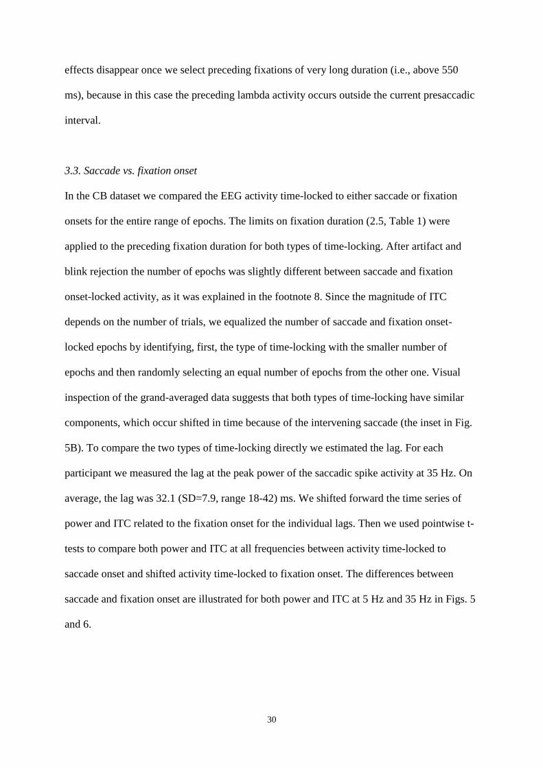
3.3. Saccade vs. fixation onset

In the CB dataset we compared the EEG activity time-locked to either saccade or fixation

onsets for the entire range of epochs. The limits on fixation duration (2.5, Table 1) were

applied to the preceding fixation duration for both types of time-locking. After artifact and

blink rejection the number of epochs was slightly different between saccade and fixation

onset-locked activity, as it was explained in the footnote 8. Since the magnitude of ITC

depends on the number of trials, we equalized the number of saccade and fixation onset-

locked epochs by identifying, first, the type of time-locking with the smaller number of

epochs and then randomly selecting an equal number of epochs from the other one. Visual

inspection of the grand-averaged data suggests that both types of time-locking have similar

components, which occur shifted in time because of the intervening saccade (the inset in Fig.

5B). To compare the two types of time-locking directly we estimated the lag. For each

participant we measured the lag at the peak power of the saccadic spike activity at 35 Hz. On

average, the lag was 32.1 (SD=7.9, range 18-42) ms. We shifted forward the time series of

power and ITC related to the fixation onset for the individual lags. Then we used pointwise t-

tests to compare both power and ITC at all frequencies between activity time-locked to

saccade onset and shifted activity time-locked to fixation onset. The differences between

saccade and fixation onset are illustrated for both power and ITC at 5 Hz and 35 Hz in Figs. 5

and 6.

31

Generally, the time courses of power time-locked to saccade and fixation onsets were quite

similar after shift correction (Fig. 5A, B), but three major differences remained (Fig. 5C)9. In

the presaccadic interval, the power at the low frequencies (5-8 Hz) was lower over the

occipital areas when the signal was time-locked to the saccade than when it was time-locked

to fixation onset (Fig. 5A, C). At the latency of the saccadic spike potential, the power at the

high frequencies (22-45 Hz) was higher when the signal was time-locked to the saccade than

to fixation onset, more prominently over the fronto-central regions (Fig. 5B). At the latency of

the lambda potential, the power over the occipital areas did not differ between the two types

of time-locking. Over the frontal regions, the power at the low frequencies was lower when

the EEG signal was time-locked to saccade than to fixation onset (Fig. 5A). This effect

occurred in the entire pre- and postsaccadic intervals except around the latency of the lambda

activity (Fig. 5C).

In ITC, time courses of both time-locking types were similar for presaccadic and lambda

activity (Fig. 6). But at the latency of the saccadic spike activity, for higher frequencies ITC

time-locked to fixation onset lagged ITC time-locked to saccade onset (Fig. 6B). In addition,

ITC magnitude for the saccadic spike activity was lower when time-locked to fixation than to

saccade onset (Fig. 6B, C). The reason is evident: with the former the variability in saccade

size produces temporal jitter for the preceding saccadic spike activity; this reduces the phase

concentration resulting in decreased ITC magnitude and a delay of its peak. The jitter affected

power to a much lesser extent (Fig. 5). We also observed some differences in ITC magnitude

at the latencies of the presaccadic and lambda activities which, however, were not systematic

across EEG channels.

9 Fig. 5C shows the intervals of significant difference obtained with FDR corrected p-values from the pointwise

ANOVAs across 15 participants; the direction of the differences can be observed in Fig. 5A, B.

32

Next, we directly compared the time courses of power and ITC for EEG activity time-locked

to fixation and saccade onsets. Fig. 7A, B illustrates the time course of power and ITC for

three frequencies: 5, 10, and 35 Hz. For all these frequencies, immediately after the baseline (-

300-250 ms) the power of the presaccadic activity decreased and ITC increased. These trends

occurred because of overlap with the preceding lambda activity: due to the 300-ms limit of

fixation duration the preceding saccade onsets were concentrated near the left edge of the

epoch. These trends disappear when a larger lower limit to fixation duration is introduced

(550 ms), as we will demonstrate in section 3.5.2.

For time-locking to saccade onset, the saccadic spike and lambda activity were characterized

by simultaneous power and ITC increases (Fig. 7A). For time-locking to fixation onset, at the

latency of the saccadic spike potential the ITC at 35 Hz suddenly dropped before rising again,

thereby delaying the ITC peak relative to the power peak. As we explained above, this is a

consequence of the jitter in onsets of the saccadic spike activity due to variable saccade size

(Fig. 6B). At the latency of the lambda wave, the power peak coincided with the ITC peak

(Fig. 7B).

We tested whether the observed discrepancy in the time course of the saccadic spike power

and ITC at 35 Hz for EEG activity time-locked to fixation onset depended on electrode

position. Fig. 7C shows the peak latencies for the saccadic spike power and ITC for frontal,

central, parietal, and occipital areas (latencies from left and right electrodes were averaged).

The ITC latency increases across areas, whereas the latency of power remains approximately

constant. We computed the lag between power and ITC peak values of the saccadic spike

activity at 35 Hz. We ran a repeated measures ANOVA on this lag with the factor

Topography (4 levels: frontal, central, parietal, occipital areas). The lag increased (F(3, 42) =

33

4.3, p = 0.02, ε = 0.82) from frontal (mean=8, SD=9.8 ms) to occipital (mean=20, SD=13.2

ms) areas. The smaller lag in the frontal than in the occipital sites indicates that EEG phase

synchronization across epochs arises earlier in sites closer to the eyes. Increasing ITC peak

latencies (Fig. 7C) reveal systematic delays in phase locking across brain regions. The

saccadic spike activity is characterized by regions of strong phase consistency across trials

which move across the scalp, from anterior to posterior. The mechanism underlying this effect

requires further exploration. The lack of a similar effect in the power peak may be due to

averaging across epochs, which may obscure latency differences across the scalp (Alexander,

Trengove, & van Leeuwen, 2015).

In sum, even though saccade- and fixation-onset time-locked activities were quite similar in

their time course (Fig. 5A, B), the former results in larger deviation from baseline than the

latter, both for power (Fig. 5C) and ITC (Fig. 6C). The largest difference between saccade and

fixation time-locking was observed for the saccadic spike activity. Presaccadic power showed

a difference over occipital areas in the low-frequencies around 5-8 Hz (Fig. 5A, C). This

suggests that the presaccadic activity should preferably be considered as time-locked to

saccade onset. We did not observe any difference between the two ways of segmentation for

lambda activity at its typical frequency about 10 Hz and in its typical location over occipital

areas. Yet, in light of previous studies showing lambda activity to be more closely associated

with fixation than with saccade onset (Billings, 1989a; Yagi, 1979) and the possibility of

different lambda subcomponents related to onset of saccade and fixation (Kazai & Yagi,

1999; Thickbroom et al., 1991), we propose that lambda activity should preferably be studied

with segmentation relative to fixation onset.

3.4. Selection of a baseline interval

34

Selection of a baseline interval is a challenge in simultaneous EEG-eye movement analysis

because different baselines allow approaching different types of brain processes

accompanying free viewing. This means that we need to base our choice of baseline on the

process we want to study. Several intervals can be offered as candidates (Fig. 8):

A common baseline interval is selected from the period of time before presentation of the

stimulus display intended for visual exploration with multiple eye movements, i.e., before the

trial onset (Fig. 8A). The common baseline is applied to all saccade-related epochs within one

trial. This type of baseline allows investigation of accumulative processes occurring across

sequential eye movements, such as memory buildup, changes in attention and effort. But the

common baseline may be located too far from the to-be-corrected epochs: between different

epochs, fluctuations can shift the ongoing EEG to different degrees. Shifts become more

likely, the longer the time interval between the baseline and the epoch, making the baseline

correction irregular and, correspondingly, unreliable.

Another option is a baseline which we call local (Fig. 8B). This type of baseline is selected

from one saccade-related epoch within a limited number of sequential epochs of interest and

applied to all these epochs. For example, a local baseline can be selected at the fixation on a

target and can be applied to the fixations on several previous and following distractors

(Körner et al., 2014). This method provides a common reference point for several sequential

processes of interest. In addition, being not too far removed from the processes of interest (as

compared to the common baseline), the local baseline is much less affected by slow ongoing

fluctuations of EEG. But in general, experimental conditions are rare, in which epochs of

interest are close to each other in a trial. This obviates a wide applicability of the local

baseline.

35

An individual baseline is selected from within some interval of a saccade-related epoch and

applied to the rest of the epoch (Fig. 8C). This type of baseline allows investigation of fast

processes that change from one saccade to another, for instance ones that are related to

perception at the current location or processes related to saccade guidance, such as attention.

Being close to the to-be-corrected epochs (typically within several hundred ms), this baseline

provides the most accurate correction and is most commonly used in co-registration research.

The individual baseline is typically set before saccade onset (Fischer et al., 2013; Fudali-Czyz

et al., 2014; Kamienkowski et al., 2012; Kaunitz et al., 2014; Nikolaev et al., 2013) or briefly

(e.g., 0-20 ms) after fixation onset (Rama & Baccino, 2010; Simola et al., 2015). In the latter

case, it is supposed that the baseline is free of EEG artifacts related to eye movement

execution, whereas activity related to visual processing (e.g., the lambda activity) has not

started yet.

Besides many advantages, the individual baseline has a major drawback: it is not exempt from

the above-mentioned issue of overlapping EEG responses (1.3). Due to the non-uniform

distribution of fixation durations, periods with high concentration of saccade-evoked activity

occur at the edges of the EEG epoch. These unavoidably contaminate any baseline interval

situated there. The result is that experimental conditions that differ in fixation duration

become incomparable. Besides this, the baseline in the presaccadic interval can be distorted if

the preceding saccades are different in size between experimental conditions, because of the

dependence of the saccadic spike and lambda activity on saccade size. Because of this

dependency, the activity evoked by the preceding saccade has a potentially confounding effect

on the following activity (which, of course, is presaccadic activity for the current saccade).

36

We will illustrate the effects of selecting an individual baseline in different intervals in the

following sections 3.5.1 and 3.5.2.

The individual baseline can be corrupted, not only by overlapping saccade-related activity but

also by activity evoked by the stimulus presentation at the beginning of a trial containing

multiple saccade-related epochs. If the saccade-related epochs associated with different

experimental conditions are distributed non-uniformly in the course of a trial, the baseline for

some of the conditions can become unreliable. This issue was raised by Dimigen and

colleagues (2011), who described how elevated brain activity right after stimulus presentation

(P300 after the sentence presentation) distorts the baseline for saccade-related epochs in one

experimental condition (low-predictability words, which tend to occur earlier in the sentence)

but not in another (high-predictability words, which tend to occur later). This prevents

comparison of the saccade-related epochs associated with high- and low-predictability words.

The suggested remedy was to exclude the saccade-related epochs within the first 700 ms after

stimulus presentation, the time needed for stimulus-evoked activity to fade out. This issue

could be relevant to our present study, because larger saccade size and shorter fixation

duration are typically observed in the beginning of free visual exploration (Findlay &

Gilchrist, 2003; Unema et al., 2005). Consequently, when saccade-related epochs are

partitioned across bins according to saccade size or fixation duration, the ones associated with

large saccades or short fixations have a higher probability of occurring in the interval

distorted by stimulus-related activity. To avoid this confounding, in the VS dataset we

excluded all saccade-related epochs which started within first 700 ms after stimulus

presentation. The analysis of the CB dataset was not affected by this issue because we

excluded the first fixation, of which the average duration was long enough (1473 ms) to

include all the stimulus-onset related activity.

37

3.5. The effects of eye movement characteristics on EEG

We now proceed to illustrate how particular differences in eye movements between

experimental conditions may distort their effect on EEG. We simulated experimental

conditions confounded with particular differences in eye movement as follows. We sorted

saccade-related epochs in an ascending order according to the eye movement characteristic of

interest and divided the sorted epochs in three equal parts, i.e., each bin contained an equal

number of epochs. This yielded a quasi-experimental design, in which each bin mimicked a

certain level of confounding by the eye movement characteristic of interest. The eye

movement characteristics of interest and their mean values in each of the three bins are

provided in Table 2 for the CB dataset and in Table S1 (in Supplementary Materials) for the

VS dataset.

Table 2. Means and standard deviations of eye movement characteristics for three bins across

15 participants for CB dataset

1st

bin 2nd

bin 3rd

bin

Preceding saccade size 17 (2.3) ms ~0.8°

29 (4.1) ms ~3.6°

47 (3.9) ms ~11.8°

Current saccade size 16 (1.9) ms ~0.8°

28 (3.1) ms ~3.6°

46 (3.8) ms ~11.8°

Preceding fixation duration with limits, ms

326 (3.6) 395 (11.4) 595 (45.8)

Preceding fixation duration, no limits, ms

177 (18.9) 285 (19.4) 483 (33.0)

Subsequent fixation duration, ms

327 (3.6) 400 (11.6) 631 (49.0)

As demonstrated in section 3.3, activity time-locked to saccade onset was similar in its time

course to activity time-locked to fixation onsets but the former was more prominent, showing

larger deviation from the individual presaccadic baseline. The data time-locked to saccade-

onset will therefore be used in most of the results below. Unless otherwise stated, effects are

38

illustrated with EEG power at 10 Hz. This is the peak frequency of the lambda activity,

which, as described in the introduction, is the main contributor to saccade-related distortion of

EEG. However, statistical results are reported for the entire 5-45 Hz frequency range.

3.5.1. Effect of preceding saccade size

To study the effect of preceding saccade size on EEG we partitioned epochs into three bins

corresponding to small, medium and large saccade size. A repeated-measures ANOVA across

15 participants on the mean power of EEG time-locked to the current saccade onset revealed

an effect of preceding saccade size on all peri-saccadic activity. The effect is most prominent

over the occipital regions. Fig. 9A shows that the following relationship appears to hold: the

larger the size of the preceding saccade, the lower the power. The blue areas in Fig. 9C mark

the intervals of significant difference between three bins.

This effect is easily mistaken for genuine, and yet it is entirely an artefact of the

methodological choices made in analyzing the data; choices that may have appeared

reasonable enough at the time. We had chosen to set the minimal fixation duration to 300 ms.

This period happens to correspond to the peak of the fixation duration distribution in free

viewing (Henderson & Hollingworth, 1999). Consequently, a large amount of the preceding

saccadic spike or lambda activity is accumulated near the left edge of the epoch. Consider that

saccade size strongly affects the saccadic spike and lambda activity. Thus, first, the shape of

the presaccadic activity is distorted proportionally to the preceding saccade size because a

larger lambda wave has a larger descending part. This effect appears in the presaccadic

activity as the initial decrease in Fig. 9A lasting from approx. -300 to -100 ms. Second,

consider we used as our baseline an interval -300-250 ms before the saccade onset, a standard

choice in EFRP research. Because the baseline interval is taken at the height of activity

evoked by, and proportional in amplitude to, the preceding saccade, baseline correction pulls

39

down all the activity after -250 ms, proportionally to the size of the preceding saccade. When

we set instead the baseline in the interval -100-50 ms before saccade onset, i.e., an interval in

which the preceding lambda activity has already faded, the entire difference disappears (Fig.

9B, D). This immediately makes clear how serious an issue in co-registration is the choice of

baseline.

3.5.2. Effect of preceding fixation duration

To analyze the effect of the preceding fixation duration on EEG we partitioned epochs into

three bins corresponding to short, medium and long fixation duration. Again we observed a

prominent effect of preceding fixation duration on all peri-saccadic activity (Fig. 10A, D).

The effect was most noticeable over the occipital areas.

This result, again, illustrates an artifact. Different preceding fixation durations push the

preceding lambda activity into different intervals of the presaccadic activity. For short

fixations (about 320 ms, Table 2), the preceding saccades occur right before the left edge of a

-300+300 ms epoch. Consequently, almost the entire interval containing the preceding lambda

activity appears within the presaccadic interval of the current saccade. For medium-length

fixations, the duration of the preceding fixation was about 400 ms on average. As a result, the

descending slope of the preceding lambda activity appeared in the presaccadic interval.

Accordingly, the presaccadic activity appears to go down. For long fixations (about 600 ms),

the preceding lambda activity ended long before the left epoch edge and the presaccadic

activity is no longer distorted.

Previous reports have shown a concentration of lambda activity in the presaccadic interval

after averaging of the saccade-related potentials (Dimigen et al., 2011). The present findings

are consistent with this observation. In addition, however, we observe that the difference in

40

duration of preceding fixation affects, not only the peak lambda frequency at about 10 Hz,

but, in fact, a large range of frequencies (Fig. 10D). Similar to those of the preceding saccade

size (3.5.1), the current effects also strongly depend on the selection of the baseline. When we

set the baseline in the interval -100-50 ms instead of -300-250 ms, again the differences

disappear (Fig. 10B, E).

Next, we estimated the effect of preceding fixation duration on the EEG, using a baseline

interval 0-20 ms after the fixation onset, similarly to Rama & Baccino (2010) and Simola et

al. (2015). In this analysis, EEG was time-locked to fixation onset and the preceding fixation

could be of any duration, whereas the subsequent fixation was longer than 300 ms (Table 1).

Not unexpectedly, we observed a large difference in presaccadic activity between preceding

fixations of different duration. In addition, we found a difference at the lambda frequency

about 10 Hz and higher, starting from about 150 ms after fixation onset (Fig. 10C, F).

In the analysis of EEG time-locked to fixation onset it is common to select a baseline interval

starting from several hundreds of ms before fixation onset (Fischer et al., 2013; Fudali-Czyz

et al., 2014; Kamienkowski et al., 2012). Fig. 10C makes it obvious that such a baseline

results in a shift of the post-fixation amplitude, if preceding fixations differ in duration

between conditions. Thus, even though the preceding fixations do not have a direct influence

on the post-fixation activity, they can affect it via the choice of the baseline.

The preceding lambda activity explains the deviation of the presaccadic power and ITC from

the baseline, which is observed for the entire range of fixation durations in Figs. 3 and 7A.

These figures were plotted using fixations of all durations within our chosen range of 300-

2000 ms. These fixations have a mean duration of 440 ms. This value is close to 395 ms

41

(Table 2), the mean duration of the preceding fixations of medium-length, corresponding to

the second bin in the analysis. This correspondence suggests that presaccadic activity in the

entire range of fixation durations can be distorted in a way similar to that by medium-length

fixations (the red curve in Fig. 10A).

To test this hypothesis we compared the deviations from the baseline for the minimal limits of

preceding fixation duration of 300 ms and of 550 ms10

(Fig. S1 in Supplementary Figures).

The limit of 550 ms was selected because it comprises of saccadic spike and lambda activity,

which lasts about 250 ms, leaving enough time for the lambda activity after the preceding

saccade to fade out before the baseline interval. The baseline interval itself was chosen at -

300-250 ms before the onset of the current saccade. The value of 550 ms was also used as the

minimum fixation duration in the visual search study by Kamienkowski and colleagues

(2012). Fig. S1 (A, D) illustrates the deviation of the presaccadic power and ITC from

baseline for preceding fixations longer than 300 and 550 ms. For fixations longer than 300

ms, the presaccadic power decreased (Fig. S1A, B) and the presaccadic ITC increased (Fig.

S1D, E) from the baseline. But neither presaccadic power (Fig. S1A, C) nor ITC (Fig. S1D, F)

deviated from baseline when the preceding fixations were longer than 550 ms. This

observation indicates that presaccadic activity is unaffected by the preceding fixation

duration, only if the presaccadic interval is longer than 550 ms.

In sections 3.5.1 and 3.5.2, we simulated experimental conditions confounded by different

preceding saccade sizes or fixation durations. This was achieved by dividing EEG epochs into

bins according to increasing values of the respective eye movement characteristics. The

10

Note that although the mean duration of the long preceding fixations (the third bin in Table 2) was 595 ms, the

individual fixations within this bin could be shorter than 550 ms, allowing some of the preceding lambda activity

to leak into the current signal. For this reason, in order to exclude the effect of the preceding fixation duration it

is not sufficient to check the absence of its effect in the third bin.

42

effects of our simulated conditions on EEG are extreme cases; they are so prominent that they

might appear trivial. However, they are helpful to guide our search for artifacts in actual

studies, where confounding by saccade size or fixation duration may be much less evident.

For example, decreasing presaccadic power as observed in medium-length fixations (Fig.

10A), or as observed in the entire range of preceding fixation durations with minimal duration

of 200-300 ms (Fig. 3A, 4B, S1A), could easily be mistaken for effects of preparing the next

saccade. But, as we discussed above, they are only effects of the preceding lambda activity.

Moreover, considering the effects reported in the sections 3.5.1 and 3.5.2 helps to build a

complete picture of the possible effects of eye movement on EEG in close vicinity of the

current saccade. This picture is important to make a judicious selection in which

characteristics of the eye movements are relevant for matching (section 3.6).

3.5.3. Effect of current saccade size

Saccade size is, amongst eye movement characteristics, probably the one with the most

profound impact on EEG. The amplitude of the saccadic spike potential gradually increases

with saccade size (reviewed in Keren et al., 2010). The increase is linear until saccade size

reaches 10° (~43 ms) (Boylan & Doig, 1989; Riemslag et al., 1988), beyond which it depends

on the initial eye position rather than on saccade size (Plöchl et al., 2012). The lambda

potential seems to depend on saccade size even if the size is larger than 10° (Yagi, 1979).

This study, however, reported statistical significance of the overall trend, but no post-hoc tests

for differences between adjacent bins for saccade sizes above 10°. In the above-mentioned

studies, saccades of predetermined sizes and restricted directions only were performed. The

effects of saccade size for the full range of saccades occurring in free viewing behavior have

not systematically been explored. We report these here for both our datasets. We considered

not only saccadic spike and lambda but also presaccadic activity. The saccadic spike and

lambda activity were measured and illustrated at the location and frequency of their maximal

43

prominence, the frontal areas (Fz-FL) at 35 Hz power and the occipital areas (O1-OL) at 5-10

Hz, respectively.

3.5.3.1. Effects in bins with equal number of epochs

We partitioned saccade size into three bins with equal number of epochs, corresponding to

small, medium and large size. The boundaries of such bins depend on the participant. The

means of three bins are given in Table 2 for the CB dataset and in Table S1 for the VS dataset.

The effects of saccade size on the saccade-related potential and EEG power time-locked to

saccade and fixation onsets are shown for the CB dataset in Fig. 11 and for the VS dataset in

Fig. S2. As expected, the saccadic spike and lambda activity were proportional to saccade

size. This dependence was much more prominent in the CB than in the VS dataset.

When time-locked to the saccade onset, the peak-to-peak amplitude of the saccadic spike

potential increased with saccade size in both the CB dataset (F(2, 28) = 69.0, p < 0.001, ε =

0.78) ( Fig. 11A, C) and in the VS dataset (F(2, 40) = 25.1, p < 0.001, ε = 0.85) ( Fig. S2A,

C). The peak-to-peak amplitude of the lambda potential increased with saccade size in the CB

dataset (F(2, 28) = 31.7, p < 0.001, ε = 0.73) (Fig. 11B, C) but not in the VS dataset (F(2, 40)

= 1.9, p = 0.16, ε = 0.85) (Fig. S2B, C). This discrepancy was also observed in power (cf. Fig.

11F and S2F), even though in the VS dataset there was a difference in power at low

frequencies (Fig. S2F), which we will explore in 3.5.3.2.

The peak latencies of the lambda potentials were shifted proportionally to the saccade

duration (Fig. 11B) (Thickbroom et al., 1991). But this shift was not visible in power (Fig.

11E), probably because of the low temporal resolution of the wavelets at 10 Hz.

44

In neither of our datasets did we observe an effect of saccade size on the power of the

presaccadic activity (Fig. 11F, S2F) and on the presaccadic potential in the CB dataset (Fig.

11A, B). In the VS dataset the saccade size effect on the mean amplitude in the -180-20 ms

interval was highly significant (the left occipital area, OL: F(2, 40) = 13.9, p < 0.001, ε =

0.91) (Fig. S2A, B). This effect, however, resulted from an interdependency between the

preceding fixation duration and the current saccade size: not only saccade size, but also

preceding fixation duration increased across the 3 saccade size bins: (F(2, 40) = 97.2, p <

0.001, ε = 0.76). The effect was similar to the one described in 3.5.2 (Fig. 10A), with the only

difference that there the range of the preceding fixation durations was substantially larger than

here: cf. the values in Table 2 with the current ones (mean and SD): 257 (14.1) ms; 269 (14.7)

ms; 289 (20.3) ms. The current effect of the preceding fixation duration on the presaccadic

potential, as in 3.5.2, was mediated by the baseline, as follows. The small saccades

correspond to the short preceding fixation durations and therefore the preceding saccadic

spike potentials occur close to the left edge of the epoch. This means that the baseline (-200-

180 ms) was taken at the peak of the saccadic spike potential. The elevated baseline level

pushes up the following lambda wave. This aggravated the distortion of the presaccadic

activity by the lambda wave (the blue curve in Fig. S2B). By contrast, large saccades are

associated with long preceding fixation durations. Therefore, for the large saccades, the

baseline happened to be taken at the trough following the preceding saccadic potential. This

resulted in a low baseline level and in a lower lambda activity (here imposed on the

presaccadic activity, the green curve in Fig. S2B). When we took the baseline in the interval -

70-50 ms before the saccade, the saccade size effect on the presaccadic potential disappeared

(F(2, 40) = 0.2, p = 0.8).

45

When time-locked to fixation onset, the peak-to-peak amplitude of the saccadic spike and

lambda potentials increased with saccade size in both datasets: the saccadic spike potential in

the CB dataset (F(2, 28) = 14.4, p < 0.001, ε = 1.0) (Fig. 11H, J) and in the VS dataset (F(2,

40) = 7.6, p < 0.002, ε = 1.0) ( Fig. S2H, J); the lambda potential in the CB dataset (F(2, 28) =

20.1, p < 0.001, ε = 0.89) ( Fig. 11I, J) and in the VS dataset (F(2, 40) = 11.2, p < 0.001, ε =

1.0) (Fig. S2I, J). These increases mainly occurred in the range of small saccades, i.e.,

between the 1st and 2

nd bins rather than between the 2

nd and 3

rd bins (Tables 2, S1), as between

2nd

and 3rd

bins there was no significance (all post-hoc p > 0.5). The dependency of power on

saccade size was observed in all frequencies11

(Fig. 11K, L, M and S2K, L, M), most

prominently in the low frequencies for lambda activity, particularly in the VS dataset (Fig.

S2L).

The saccade size effect apparent in the presaccadic interval about 100 ms before the fixation

in both datasets (Fig. 11M, S2M) can be understood as an effect of the saccade size effect on

the current saccadic spike activity spilling out due to the low temporal resolution of the

wavelets at low frequencies.

3.5.3.2. Effects across frequencies

We found a saccade size effect across all EEG frequencies studied (Fig. 11F, M, S2M).

Saccadic spike activity is most prominent at frequencies about 60-90 Hz (Keren et al., 2010)

and lambda activity is most prominent at frequencies around 10 Hz (Ossandón et al., 2010,

Fig. 3A, 4B, E).

11

At the lambda frequencies (10-22 Hz), about 100 ms after saccade or fixation there was a gap in time, in which

we cannot see the saccade size effects (Fig. 11F, M, S2M). This occurred because the ascending slopes of the

lambda activity for saccades of different sizes overlapped.

46

We computed the difference in power between the 3rd

and 1st bins for ten frequencies, from 5

to 45 Hz (Fig. 11G, S2G) at the maxima of saccadic spike and lambda power. For saccadic

spike activity, the maximum was found over the frontal areas (Fz or FL) in the -100+100 ms

interval from saccade onset and for the lambda activity over the occipital areas (O1 or OL) in

the 75-200 ms interval from fixation onset. For the saccadic spike activity the power

difference was highly significant (all p < 0.008, one-sample t-tests against 0) and gradually

increased with frequency in both datasets (Fig. 11G, S2G). This finding suggests that the

frequencies of maximal prominence of the saccade size effect may correspond to those of the

maximal prominence of saccadic spike activity. The latter frequencies, however, lie above the

5-45 Hz range of our study. No such correspondence was observed for the lambda activity:

for both datasets the largest difference between the 3rd

and 1st bins occurred at the lowest

frequency of 5 Hz. For the CB dataset the difference gradually decreased with frequency (Fig.

11G) and was highly significant for all frequencies (all p < 0.001, one-sample t-tests against

0). For the VS dataset a difference was observed for 5 Hz (t(20)=6.5, p < 0.001) and 6 Hz

(t(20)=4.3, p < 0.001), but not above these frequencies (Fig. S2G).

3.5.3.3. Effects of absolute saccade size

The division of saccades into three size bins with equal number of epochs allowed us to

consider individual differences in saccade size distributions, because the bin boundaries

depend on the participant. To test the effect of absolute saccade size on EEG irrespective of

individual saccade size distributions, in the CB dataset we partitioned saccade duration into

four bins with equal ranges: 0-15, 15-30, 30-45, 45-60 ms (i.e., approximately 0-0.8, 0.8-4, 4-

11, 11-18°). The number of epochs was equalized across bins by first identifying the bin with

the smallest number of epochs before filling the other three bins with the same numbers of

epochs by randomly selecting from the available ones. The dependence on saccade size was

47

tested for the peak-to-peak amplitude of the saccadic spike and lambda potentials, as well as

for the mean power at 35 Hz in the interval from -10 to 30 ms relative to saccade onset for the

saccadic spike activity and at 10 Hz in the interval from 100 to 180 ms relative to saccade

onset for the lambda activity. Fig. S3 shows the effect of saccade size on the saccade-related

potentials and EEG power for the CB dataset.

As expected, the effect of saccade size on the saccadic spike activity was highly significant

for the peak-to-peak amplitude (F(3, 42) = 47.2, p < 0.001, ε = 0.67) as well as power (F(3,

42) = 41.8, p < 0.001, ε = 0.81) (Fig. S3A-C). The amplitude and power prominently grew

across bins up to and including the 3rd

bin, which comprised saccades of 30-45 ms duration

(~4-11°). In the 4th

bin the amplitude and power appeared higher than in the 3rd

bin but the

post-hoc test showed no significance. The absence of a difference between 3rd

and 4th

bin is

consistent with the observation that for saccades larger than 11.5° the saccadic spike potential

does not depend on saccade size (Plöchl et al., 2012).

There was a prominent effect of saccade size on the lambda activity for amplitude (F(3, 42) =

29.0, p < 0.001, ε = 0.55) as well as for power (F(3, 42) = 16.9, p < 0.001, ε = 0.81) (Fig.

S3D-F). The activity prominently grew across bins, up to and including the 3rd

bin, appearing

even to drop in the 4th

bin. Yet the post-hoc test did not show a difference between the 3rd

and

4th

bins, neither for amplitude nor power, nor between the 1st and 2

nd bins for power. Thus,

our findings contradict Yagi’s (1979) suggestion that the dependency of lambda activity on

saccade size extends to saccades larger than 10°.

In sum, both for saccade and fixation time-locking, the saccadic spike and lambda activities

strongly depend on saccade size. However this dependency is confined to a relatively limited

48

range of saccade sizes; it flattens out for larger saccades. For saccadic spike activity the

dependency increases with frequency, suggesting correspondence to the frequency of

maximal prominence of this activity. By contrast, for the lambda activity the dependency is

largest at low frequencies and does not correlate with the frequency of maximal prominence.

We did not find an effect of saccade size on the presaccadic activity. We demonstrated,

however, that sequential dependency between current saccade size and preceding fixation

duration may distort the presaccadic potential via incorrect baseline selection.

3.5.4. Effects of current saccade direction

To study the effect of saccade direction we partitioned the EEG epochs into four saccade

direction quadrants: up, down, right, left. Saccades, except strictly vertical ones, are

lateralized movements, which are reflected in different topography of the saccadic spike

activity over the left and right frontal areas (Csibra et al., 1997; Keren et al., 2010; Moster &

Goldberg, 1990; Plöchl et al., 2012). We evaluated the peak-to-peak amplitude and the mean

power in the –10 +30 ms interval at 35 Hz of the saccadic spike activity at the left and right

frontal electrodes (F3-F4 or FL-FR in the CB and VS datasets, respectively). We also

evaluated the lambda activity in the left occipital electrode (O1 or OL). For this we obtained

the peak-to-peak amplitude and the mean power in the 100-180 ms interval at 10 Hz, as

before. Both activities were time-locked to saccade onset. Since we used the mastoid

reference in CB dataset but the average reference in VS dataset, the results are presented for

the two datasets separately.

For the CB dataset, the amplitude and power of the saccadic spike activity over the left frontal

area were smaller for left than for right saccade directions (all p < 0.03, pairwise t-tests) (Fig.

12A, D, G). A tendency to the opposite over the right frontal area (Fig. 12B, E, G) did not

reach significance. For up-down saccade directions, the amplitude and power over both frontal

49

areas were larger for the down than for the up direction (all p < 0.001, pairwise t-tests) (Fig.

12A, B, D, E, G). The topography of the saccadic spike activity for the leftward and rightward

saccades as well as the larger amplitude for the down than for the up direction were similar to

those found by Plöchl et al. (2012) using a nose reference. However for recordings referenced

to the posterior electrodes, larger amplitude has been reported for the up than for the down

direction (Keren et al., 2010; Thickbroom & Mastaglia, 1986).

For the VS dataset, the amplitude and power of the saccadic spike activity over the left frontal

areas were opposite to that of the CB dataset: larger for left than for right saccade directions

(all p < 0.004, pairwise t-tests) (Fig. S4A, D, G); whereas the amplitude and power over the

right frontal areas were larger for the right than for the left direction (all p < 0.003, pairwise t-

tests, see Fig. S4B, E, G). The topography was similar to that found using an average

reference (Csibra et al., 1997) as well as using a posterior reference (Keren et al., 2010).

There was no difference between the up and down saccade directions.

For the lambda activity, we found no systematic effects of saccade direction, although there

was a difference in amplitude of the lambda potential between up and down directions which,

however, was opposite in direction for the CB and VS datasets (Fig. 12C, F and S4C, F) and

was not supported by a power difference.

Saccade size and direction can be interdependent (Tatler & Vincent, 2008). Because of this, in

principle, saccade size might explain saccade direction effects. We established a relationship

between saccade duration and direction in both our datasets: the saccade duration was

considerably longer for the down than the up direction (all p < 0.001, pairwise t-tests) (Fig.

12G and S4G), similarly to Tatler and Vincent (2008). This difference corresponded to the

50

larger amplitude of the saccadic spike activity for the down than for the up direction in the CB

dataset, reported above. Moreover, the saccade duration was significantly longer for the left

than the up direction in both datasets (all p < 0.002). However this effect had a counterpart in

EEG only over the right frontal area in the CB dataset, and neither over the left frontal area in

the CB dataset nor in the VS dataset. These findings indicate that the effects of saccade

direction on the saccadic spike activity cannot completely be explained by saccade size.

Amplitude and topography of the saccadic spike activity depend on initial eye position rather

than on saccade size (Plöchl et al., 2012). This may explain the inconsistent effects of saccade

size and direction.

In sum, saccade direction affects amplitude and topographical distribution of the saccadic

spike activity. However, the direction of these effects is strongly dependent on the choice of

reference electrode. We observed no effect of saccade direction on lambda activity. But since

size and direction are correlated, and because saccade size prominently affects the lambda

activity, a possible confounding cannot completely be excluded.

3.5.5. Effects of subsequent fixation duration

We tested whether the duration of the subsequent fixation has an effect on the lambda activity

and the following postsaccadic activity. Since the lambda wave is time-locked to fixation

rather than saccade onset (Billings, 1989a; Yagi, 1979), for this analysis we segmented EEG

epochs relative to fixation onset. Also, in contrast to the previous analyses we limited the

duration of the subsequent rather than the preceding fixation interval (the effective range of

the subsequent fixation duration was 300-2000 ms in the CB dataset and 200-1000 ms in the

VS dataset). We partitioned subsequent fixations into three duration bins corresponding to

short, medium and long fixation durations (see the means in Table 2 for the CB dataset and in

Table S1 for the VS dataset).

51

In the CB dataset the subsequent fixation duration effect arises in the interval 250-300 ms

after the onset of the current fixation (Fig. 13). EEG power at the frequencies 5-17 Hz was

higher for shorter than for longer fixation durations (Fig. 13C, E). This effect was observed

only in frontal (Fig. 13A, C) and not in occipital (Fig. 13B, D) sites. This means that it cannot

be attributed to the lambda activity. Most likely, the effect was related to the initiation of the

subsequent saccade, as it occurred over the frontal areas and was most visible for subsequent

fixations of short duration (Fig. 13A, C), i.e., when a subsequent saccade started immediately

after the end of an epoch. Its occurrence at the low frequencies could be explained as spilling

out of subsequent saccadic spike activity, a consequence of the low temporal resolution of

low-frequency wavelets. Remarkably, the low-frequency effect at the right edge of the epoch

was observed even though a restriction to minimal durations of 300 ms was imposed on

epochs carrying the subsequent fixation. Thus, a minimal epoch duration does not secure

against effects at the edges of epochs if these epochs differ systematically in fixation duration.

In the VS dataset we did not observe any effects of subsequent fixation duration on EEG (Fig.

S5), even though there was a tendency similar to the CB dataset (Fig. 13A, C) at the right

edge of the epoch. Consistent with the CB dataset, the tendency suggested higher amplitude

for short than for medium and long subsequent fixation durations (Fig. S5A, C).

We conclude that subsequent fixation duration has a small effect at the right edge of an EEG

epoch. The effect may play a confounding role in time-frequency analyses involving low-

frequency EEG.

3.6. Matching eye movement characteristics before EEG analysis

52

Averaged saccade-related EEG may be distorted by both saccadic spike and lambda activity

from preceding as well as following epochs, because of the non-uniform distribution of

fixation durations. Moreover, the presence of sequential dependencies between eye

movements (Tatler & Vincent, 2008) suggests that some eye movement characteristics may

distort EEG indirectly. Regression-based methods cannot eliminate the distortions, because

they can barely be separated from the signal and because of problems in applying regression

methods to serially-dependent data. To remedy this problem, we will advocate a strategy of

selecting across experimental conditions those EEG epochs that are matched according to

their eye movement characteristics (Devillez et al., 2015; Dias et al., 2013; Dimigen et al.,

2011; Fischer et al., 2013; Kamienkowski et al., 2012). Matching does not remove the

distortions but balances them across conditions. Note, however, that matching is conservative;

it may flatten or distort the difference of interest, between perceptual or cognitive processes.

This may occur because matching changes distributions of eye movement characteristics and

corresponding saccade-related epochs. Since epochs with unmatched characteristics may

contain information about the condition in the most conspicuous form, removing such epochs

makes information in the remaining epochs more similar between conditions.

The matching procedure we propose involves a selection of eye movements which lie close in

a space, in which the dimensionality is defined by the number of characteristics to-be-

matched. For example, eye movements may be matched by minimizing the quadratic distance

between them in the space of considered characteristics, which is normalized by the sum of

their standard deviations (Kamienkowski et al., 2012). Below we will describe a matching

procedure which involves finding the Mahalanobis distance across various eye movement

characteristics. This procedure was initially proposed by Dias and colleagues (2013), who

applied it for equalization across a large set of eye movement characteristics. Their study

53

involved few targets and numerous distractors. Consequently, they were able to find matches

for targets among a large amount of distractors. Such a large difference in number, however,

does not usually occur between trials of experimental conditions. As a result, it may be

difficult to match all eye movement characteristics. We discuss guidelines for selectively

matching eye movement characteristics, depending on the activity of interest in section 4.8.

3.6.1. Matching procedure

Step 1 – Selection of distance measure

The Mahalanobis distance (MD) is a measure of the distance between a data point and the

center of the covariance space of a multivariate distribution. This measure can be used to

match data points across various eye movement characteristics such as saccade size, fixation

duration and saccade direction in two or more experimental conditions. The distributions of

eye movement characteristics like saccade size and fixation duration are typically non-normal.

In such distributions, the effect of outliers or inflated standard deviations on the MD measure

may cause the resultant matching to be unreliable. In that case an alternative is to use the

rank-based Mahalanobis distance, wherein effects of non-normality are mitigated. Below we

detail the matching procedures based on both of these measures.

Step 2 – Cutoff based elimination

The cutoff distance is selected via an iterative procedure. First, an arbitrary cutoff distance is

selected. All data points that lie within this cutoff distance are considered as candidate

matched data points. Fig. 14A illustrates this procedure for two experimental conditions

across three eye movement characteristics: saccade size, fixation duration and saccade

direction. The points that lie above the cutoff distance and, are hence, eliminated, are crossed

out. Cutoff distance is reselected if the conditions are not matched (Step 3).

54

Step 3 – Verification of matching procedure

To verify that the eye movements are successfully matched, we have to show that matched

data points have similar eye movement characteristics. This may be done by showing no

difference between conditions using a statistical test of significance12

. If eye movement

characteristics are different, the cutoff distance is reduced and Step 2 is repeated. This

iterative process of cutoff selection is done until the verification test shows the conditions to

be no longer different.

3.6.1.1. Procedure based on Mahalanobis distance

In this procedure, the Mahalanobis distance of each data point (eye movement characteristic)

is computed from a reference distribution. This means a reference distribution has to be

selected first. The reference distribution may be one of the experimental conditions or a

pooled distribution of conditions. If the total number of data points across experimental

conditions is N, we compute N distance measures from the reference distribution. For each

multivariate data point, xi, for i = 1, … , N, the MD from the reference distribution with

covariance matrix, S, and mean, µ, is computed as

=

The mean and variance are not ideal measures of the center and spread of the Mahalanobis

space, since eye movement characteristics are typically not normal. However, for the purpose

of finding data points that lie close to each other across multiple dimensions, selection of the

12

As it may be argued that not being able to show difference in a statistical test does not mean sameness, we

considered a test of equivalence (Wellek, 2010) as an alternative. Equivalence tests are commonly used to show

similarity between groups in clinical or pharmaceutical applications. Equivalence tests require the selection of an

equivalence interval based on criteria relevant for practical use and the test statistic in use. We found an

equivalence test unfit for our matching procedure because of the unavailability of standards or recommendations

to establish equivalence of eye movements suitable to our purposes.

55

appropriate cutoff MD circumvents the problem of non-normality. An appropriate cutoff

maybe selected as an arbitrarily high percentile, e.g., 99th

, of the distribution of all MDs.

3.6.1.2. Procedure based on rank-based Mahalanobis distance

The rank-based MD (Rosenbaum, 2005) computes the distance between any two data points

based on their rank in the distribution. First, the experimental conditions are pooled to give a

common distribution of size N. Then, each parameter or covariate is replaced by its rank or

the average rank in case of ties. For this ranked distribution with covariance matrix, S, an

adjusted covariance matrix is computed using the formula

where Rdiag is a diagonal matrix of which the diagonal elements are computed as the ratio of

the standard deviation of the untied ranks of the covariates to the tied ranks of the covariates.

Now, the rank-based MD between any two data points, xi and xj, for i, j = 1, … , N, in the

ranked distribution is computed using the formula

The total number of distances computed is now (N×(N-1))/2 because the measures are

obtained between each data point and every other data point and not between each data point

and the distribution. Therefore, after selection of a cut-off value, the elimination procedure is

two-step. First, the cutoff is fixed at a high number, e.g., 95. From this two cutoff values are

determined – the cutoff MD and the proximity cutoff. The cutoff MD is computed as the 95th

(cutoff) percentile from all the MDs obtained. The proximity cutoff is computed as 95 (cutoff)

percentage of the total number of points from which the distance of each point is calculated,

that is, (N - 1)*(cutoff/100). For example, if N = 100, the proximity cutoff is 94 for a cutoff

56

value of 95. The final set of points are selected as those points that have a rank-based MD less

than the cutoff distance from at least as many points as the proximity cutoff.

3.6.1.3. An example application of the matching procedure

We illustrate the matching procedure with an example using high-order properties of the

scenes in our CB dataset. The stimulus images were classified according to the interest of the

observer in the part of the scene subject to change: central or marginal. The classification of

each image was determined by Rensink and colleagues (1997), who provided us with the

image dataset. For one participant, we compared fixation duration, size and direction13

of the

preceding saccade between these two conditions. The number of eye movements in the central

interest condition was 382 (n1) and in the marginal interest condition was 423 (n2). In

separate t-tests we found significant differences (p < 0.05) for fixation duration and saccade

size. Each t-test had a power of 0.8 for a small effect of size d = 0.2 (J. Cohen, 1988). Since

the data appear non-normal, we additionally confirmed the difference using separate

permutation tests. We resampled the data 1000 times using the Monte Carlo method and

found the difference between means each time. At the 5% significance level, the conditions

were significantly different for fixation duration and saccade size, in agreement with the t-test

results.

Data points for computing MD were defined with three eye movement characteristics:

fixation duration, saccade size and saccade direction. Saccade direction was included for

illustration purposes, even though fixations did not differ on this characteristic between

conditions. Data points were then matched across these three characteristics based on both the

MD and the rank-based MD. For MD computation, the data points of the central interest

13

To make saccade directions comparable by accounting for circularity, for each saccade, a vector was drawn

from the saccade origin to its destination. The cosine transformed slope of this vector was used as a placeholder

for saccade direction.

57

images were used as the reference distribution. The initial cutoff was set at the 99th

percentile.

The data points that lay above the cutoff were removed. Then we compared the eye

movement characteristics of the two conditions for the remaining data points using separate t-

tests. If the t-tests found no difference, this result was confirmed by permutation tests to

account for the effect of non-normality of the distributions of eye movement characteristics. If

either the t-test or the permutation test showed a difference, we reduced the cutoff and

repeated the process. Once both tests no longer showed a difference, we stopped the process

and considered the eye movement characteristics as matched between conditions. For the

rank-based MD, the groups were matched at a cutoff value of 99, while using the MD,

matching was attained at a cutoff value of 8714

. After matching, the number of data points

reduced to n1 = 332, n2 = 384 in the rank-based MD procedure and n1 = 299, n2 = 403 in the

MD matching procedure. As shown in Fig. 14B, after matching the distributions of the eye

movement characteristics are less skewed and more uniform than before.

Power analysis of the t-test on the final set of matched data points showed that a small effect

(d = 0.2) could be detected with a probability of 0.76 for MD and 0.74 for rank-based MD.

Since the power of the test is close to the recommended 0.8 for detecting even small effects (J.

Cohen, 1988), we could assume that the conditions were similar across eye movement

characteristics. Thus, in our case there is no advantage of either the MD or rank-based MD.

The rank-based MD may be preferable in case of highly skewed distributions, where using

MD fails to find a match or results in too small numbers of remaining data points. Generally

speaking, the non-normality of eye movement distributions suggests the existence of datasets

for which rank-based MD matching could be preferable.

14

For matching using MD, the cutoff value refers to the (87th

) percentile of distances, whereas when using rank-

based MD, the cutoff value of 99 refers to both the 99th

percentile of distances and 99% used to compute the

proximity cutoff.

58

To verify matching of conditions, a significance test can be used if the sample size is large

enough to afford reasonable power (> 0.8) to the test. In the example above, the sample size is

very large, so the tests are likely to be overpowered and detect very small effects. Typically,

the sample sizes (number of epochs) in EEG analyses are smaller. In the case of a sample size

of, e.g., 200 (100 epochs per condition), the power of a t-test would only be 0.3 for detecting

small effects (d = 0.2). But, this test still has a power of 0.8 for medium-sized effects (d =

0.4). Therefore, for such sample sizes (200), it is still reasonable to assume conditions to be

equal if a t-test shows no statistical difference. For smaller sample sizes, matching cannot be

reliably verified using a t-test as it would be underpowered to detect effects of medium size (d

= 0.4).

Ideally, in combined EEG-eye movement analyses the effect size optimal for verification of

matching should be derived by quantifying the effect of eye movement characteristics on

EEG. That is, if a small or medium difference in eye movements (d = 0.2 or d = 0.4) results in

changes of EEG within its signal-to-noise ratio, then selection of the effect size can be more

liberal (e.g., d = 0.8). However, the choice of an optimal effect size based on the effect of eye

movement characteristics on EEG requires meticulous modeling, which should be a subject of

future research.

4. General discussion

Co-registration of EEG-eye movement in free viewing conditions has possibilities as well as

pitfalls. We examined two datasets which differed in stimulus, task, and EEG recording

system, but shared a paradigm involving extensive saccadic exploration of a stimulus display.

With these datasets we showed how to analyze evoked potentials, time-frequency

decompositions, and inter-trial coherence of the main peri-saccadic EEG activity. We

59

compared time-locking of EEG segments to the saccade and fixation onsets and discussed

different types of baseline correction. However, the major part of our paper was dedicated to

the central problem and possible solutions of overlapping EEG responses due to sequential

eye movements. Below we will expound our observations and provide some further

recommendations for planning and running experiments.

4.1. Stimulus properties

To maximize the benefit of co-registration in free viewing, stimuli should preferably be large.

The area within which visual stimuli can be placed (the display area) is limited by the

maximal excursion of the eye within the head (the oculomotor range), which is about +/-50°of

visual angle (Guitton & Volle, 1987; Stahl, 1999). However, since people tend to start

rotating the head when saccades exceed 20° (Fuller, 1992), this value should be the basis for

determining maximum display size. Twice this amount (40°), because saccades without head

movements could then be made in opposite directions, would be a suitable upper bound for

the display size.

If the study is aimed at saccadic exploration of stimuli, the size of each should be larger than

the fovea, which has a diameter of about 1° of visual angle around the fixation point (Findlay

& Gilchrist, 2003). Spatial separation between stimuli is delimited by visual acuity, which

markedly decreases with distance from the fovea. In the parafoveal region (up to 5° of visual

angle around the fixation), stimulus information can still be partially processed and encoded

(Findlay & Gilchrist, 2003). In natural scenes the size of stimulus region and stimulus

separation are beyond the grasp of the experimenter, whereas in artificial displays these can

be fully controlled. For example, in the VS experiment, a display item was 0.41° in size and

the minimal distance between them was set to 3.12°. Since this distance was still within the

60

parafoveal region, we encircled each item to complicate discrimination, such that it would

require fixation (Körner & Gilchrist, 2007; Peterson & Gibson, 1991). As a result, fixations

could unambiguously be attributed to targets or distractors (Meghanathan et al., 2015).

Luminance is another stimulus display property that requires control. Luminance difference

between saccadic start and end points may have an effect on lambda activity (Ossandón et al.,

2010). Since lambda activity may indirectly (e.g., via baseline, see 3.4) affect the entire peri-

saccadic activity, we would recommend that fixation targets have equal luminance. This can

easily be achieved for artificial displays but is difficult to obtain with natural scenes. In that

case, it should be ensured that luminance at the fixation locations of interest is comparable

between conditions.

4.2. Number of trials

In free viewing, observers make about 3-4 saccades per second. During a one-hour

experiment one can collect more than 10,000 saccade-related EEG epochs, which might seem

more than enough for eliciting robust saccade-related potentials, even if the number of

experimental conditions is large. However, in practice, loss of saccade-related epochs during

pre-processing is typically much higher in a co-registration study than in a classical ERP

study. In addition to classical exclusion factors such as incorrect responses, eye movement

and EEG artifacts, exclusion factors specific for co-registration, such as non-target fixations,

short fixations (see below) should be taken into account. Moreover, the saccade-related

epochs within the first 700 ms after the stimulus onset should be excluded because they may

be affected by the stimulus onset-related potential (Dimigen et al., 2011). In addition, we lose

the unmatched epochs rejected in the matching procedure we recommended for controlling

overlapping effects of sequential eye movements.

61

The percentage of rejections should be assessed in advance in pilot experiments and pilot

analyses. The number of accepted saccade-related EEG epochs per condition should

approximately be the same as in ERP studies, because it is generally believed that the main

components of the saccade-related potentials are similar to those in ERP. For instance, Luck

(2005) recommends having 60 trials for large late components (e.g., P3 or N400), and

hundreds of trials for small, earlier components. In co-registration analysis, the saccadic spike

potential is already visible after averaging of several tens of epochs. The lambda potential

requires averaging of more epochs, which number, however, depends on the luminance range

within the stimulus display, as illustrated by the noticeable difference in lambda amplitude

between our two datasets. If the matching procedure is applied, a minimum of approximately

100 epochs per condition after rejection is needed to verify matching quality (3.6.1.3).

4.3. Synchronization of stimulus presentation and EEG-eye movement recordings

A typical EEG-eye movement co-registration setup consists of three components: a computer

with a monitor for stimulus presentation, an EEG recording system and an eye tracking

system. Synchronization of events across these three components, via markers, is a crucial

step in the preparation of a co-registration study. Since synchronization markers cannot be

inserted after the recording, the researcher has to ascertain beforehand the proper functioning

of the synchronization of all components. There are several methods for achieving this.

The most straightforward and reliable way is a common trigger which is sent as a TTL pulse

from the presentation computer simultaneously both to the EEG and eye tracking systems.

This requires a splitter connected to a parallel port output of the presentation computer15

. We

15

Note, however, that modern computers often no longer have an inbuilt parallel port and hence a parallel port

card may have to be additionally installed.

62

used this method in recording the VS dataset. Due to slow drift of the component clocks,

during a one-hour experiment, the difference between clocks may reach several hundreds of

milliseconds. A single TTL pulse at the beginning is not sufficient for avoiding

desynchronization during the experiment. Instead, a TTL pulse should be sent at the onset of

every single trial, to keep the difference between the clocks small enough, typically in the

order of 1-2ms for a 10s trial.

The second synchronization option involves the output of the eye tracking system. Eye

position is typically output as an analog voltage. Via a digital-to-analog converter, it is fed to

the EEG recording system, where it appears as a separate channel in the recording. We

applied this method of synchronization for the CB dataset.

Thirdly, the growing popularity of EEG-eye movement co-registration has recently led major

producers of EEG and eye tracking equipment to develop synchronization tools for their

systems. For example, Electrical Geodesics Inc. (Eugene, OR) offers a timing device called

“Network Time Protocol”. This mechanism allows streaming of stimulus markers and eye

movement events directly into the EEG recording software in an online fashion via TCP/IP

communication.

Since synchronization of events is achieved via markers sent to the eye movements and EEG

systems, it is not necessary to record data with the same sampling rate for both systems.

However, it is recommended that the sampling rates be equalized by downsampling the data

with the higher sampling rate, since data processing becomes easier when both EEG and eye

tracking data have the same number of data points.

63

4.4. Inclusion of EOG electrodes

In EEG-eye movement co-registration, when the eye movement signal is collected via eye

tracking, EOG recording may seem to be redundant. In fact, however, the eye tracking and

EOG information are complementary: eye tracking allows precise detection of the eye events,

whereas EOG is helpful as an additional input for ocular artifact correction. In contrast to the

traditional ERP study, where EOG is mostly used for correction of blink-related artifacts, with

co-registration correction of blink effects on EEG is impractical, because blinks are

accompanied by transient downward and nasalward eye movements of about 1-5° (Collewijn,

van der Steen, & Steinman, 1985). This may create spurious saccade onset signals, rendering

saccade-related EEG segmentation inaccurate. In other words, a blink makes it uncertain

whether the pervious fixation interval continues after the blink. Moreover, blinks cause large

disturbances in EEG amplitude that take significant time to return it to the baseline. Blinks

can easily be identified using eye tracking information. Based on this information, the EEG

segments between a blink and both the preceding and the following saccade should thus be

removed. For example, we excluded saccades and, correspondingly, saccade-related EEG

segments if a blink occurred within -300 to 300 ms relative to saccade onset.

Main artifacts, which should be corrected in co-registration, are produced by rotation of the

corneo-retinal dipole and by constriction of ocular muscles. EOG recording is mandatory for

correction of these artifacts if the regression-based correction methods are used (Romero et

al., 2008). But for methods based on blind source separation, such as Independent Component

Analysis (ICA), EOG recording is not strictly necessary, because both EOG and EEG are

mixtures of ocular and brain signals. EEG, particularly over the frontal sites, contains a large

portion of EOG activity (Ma et al., 2011; Romero et al., 2008). Yet, there is a benefit in

having EOG recordings as input to ICA. Correlation of independent components with EOG

64

may facilitate their attribution to ocular artifacts, which is the main difficulty in ICA-based

artifact correction. The advantage of using EOG recordings as input to ICA was illustrated by

the smaller amplitude of the saccadic spike activity in the VS dataset, which included EOG

electrodes, than in the CB dataset, which did not have them.

4.5. Running a co-registration experiment

Efficient preparation and smooth running of a co-registration experiment is greatly enhanced

by the cooperation of two experimenters: one responsible for the EEG recording and another

for the eye tracking. While the duty of the EEG experimenter consists mainly in the setup and

adjustment of EEG electrodes prior to the experiment, with only monitoring of the recording

quality needed during the experiment, the work of the eye tracking experimenter continues

throughout its course. Video-based eye trackers require a calibration procedure before eye

tracking to compute a calibration model in order to establish where on the screen the

participant is fixating. The accuracy of this measurement decreases with time for reasons such

as participant head movements and drift, i.e., slow movements of the eyes. Typically, the eye

tracking software provides drift correction functionality to adjust the calibration model for

drift as long as error values are small. This functionality maybe used before each trial. If error

is greater than a threshold value, e.g., 2°, drift correction cannot proceed and calibration has

to be repeated. In addition, a mandatory re-calibration should be done every 5 or 10 minutes

to avoid large errors caused by drift and/or errors introduced by participant head movements.

Therefore, in co-registration experiments it is essential to present trials in blocks, in order to

allow for re-calibration breaks every 5-10 min.

4.6. Software

65

Processing of eye movements and EEG data together has often been done using custom

software written in MATLAB, Python or other languages. In the last few years, software

packages and modules have been developed to make this task easier. The ‘Add Channels’

module for processing co-registered data is available as part of BrainVision Analyzer version

2.0.3 and later. Currently, this module accepts eye tracking data from SMI, Tobii, ADL, and

SR EyeLink 1000 Plus systems. It allows the synchronization of triggers between EEG and

eye tracking data and can also identify eye events like saccades and fixations. For MATLAB

users, the EYE-EEG extension for EEGLAB has been developed. This extension not only

enables synchronization of EEG and eye tracking data as well as saccade and fixation

detection, but also provides additional functions such as data removal based on eye position,

the ocular artifact correction procedure proposed by Plöchl et al. (2012) (see 1.2), analysis of

saccade-related activity in both the time and frequency domain (http://www2.hu-

berlin.de/eyetracking-eeg, Dimigen et al., 2011).

4.7. Excluding segments associated with short fixations

There is no consensus among researchers regarding the exclusion of segments associated with

short fixations. Some refrain from excluding them altogether (Dias et al., 2013; Körner et al.,

2014; Simola et al., 2015; Simola et al., 2013), others exclude segments associated only with

short (50-100 ms) fixations (Devillez et al., 2015; Dimigen et al., 2011; Graupner et al., 2007;

Ossandón et al., 2010; Rama & Baccino, 2010), still others exclude segments associated with

fixations shorter than the mean of the fixation duration distribution (Fischer et al., 2013;

Fudali-Czyz et al., 2014; Nikolaev et al., 2013; Nikolaev et al., 2011), or consider for analysis

only segments associated with extremely long (>500 ms) fixations (Kamienkowski et al.,

2012; Kaunitz et al., 2014).

66

Exclusion of short fixations and associated EEG segments aims to meet several important

goals, such as estimating perceptual or cognitive processes that are completed within one

fixation interval, e.g., allocation of attention to the next fixation target (Hoffman &

Subramaniam, 1995). In addition, it may appear that exclusion enables time-frequency

analysis which, in order to be reliable, requires a minimum number of EEG cycles. Likewise

apparently, it permits “clean” EEG epochs, i.e. epochs that contain neither saccadic spike nor

lambda activity evoked by adjacent eye movements. However, as we demonstrated in section

3.5, efforts to achieve these aims through exclusion are moot. Because of the non-uniform

distribution of fixation durations, no exclusion criterion can prevent, on the one hand, the left

edge of an EEG epoch from being distorted by lambda activity related to the preceding

saccade and, on the other hand, the right edge from being distorted by saccadic spike activity

related to the subsequent saccade. Thus, exclusion criteria based on fixation duration are not

sufficient to reduce the influence of sequential eye movements on EEG.

Another caution about exclusion is the significant loss of data. For example, we lost about

60% of segments when we set the lower limit of fixation duration to 300 ms for the CB

dataset and to 200 ms for the VS dataset, resulting in considerable reduction in the power of

subsequent statistical analysis. Finally, removing data may impoverish or bias information

about perceptual and cognitive processes in the dataset. For instance, short fixations may have

a particular role in visual processing: they may occur during a fast initial exploration of the

scene (Unema et al., 2005). Eliminating short fixations may, therefore, bar us from studying

the dynamics of visual exploration.

Decisions about exclusion could still be motivated by assumptions about the processes of

interest. For example, exclusion of short saccade-related epochs will absolutely be necessary

67

when focusing on visual processes that start around the time of a saccade and finish within a

fixation interval, because intervening saccades may disrupt these processes and distort the

corresponding EEG activity. Consider, for instance, an experiment which aims to analyze

lambda activity as an indicator of early visual processing. A lambda wave has a peak latency

of 100 ms after fixation onset and returns to baseline after about 200 ms. If the next saccade

starts at 50 ms, the lambda wave will be disrupted. However, exclusion may not be necessary

for analysis of high-order processes, which involve sampling and accumulation of information

from many locations of a scene and are reflected in the late evoked components. If the

fixation durations are matched between conditions, the disturbing effect of intervening

saccades on the current EEG segment could be ignored, with constraints discussed in 1.4.

Once the decision to exclude short fixations has been made, the next step is to determine the

appropriate minimal fixation duration. If the analysis aims at long EEG epochs for studying

late components, it will be unaffected by the choice of threshold. If, however, epochs should

in their entirety lay within a single fixation (as in our analyses), the threshold value should be

set so as to allow epochs to be as long as possible and retain as large a number of epochs as

possible in the dataset. The optimal minimal duration thus should be found to the left side of

the peak in the fixation duration distribution. The numerical value depends on fixation

duration distribution, which varies according to the task and the display used. Average

fixations were longer in the CB dataset than in VS dataset, as typically fixation durations are

longer in scene memorization than in visual search tasks (Castelhano, Mack, & Henderson,

2009; Henderson, Weeks, & Hollingworth, 1999) and longer for color photos with many

details (i.e., with a wide range of spatial frequencies) than for line drawing (Findlay &

Gilchrist, 2003). Low-level properties of the display may also affect fixation duration, such as

luminance and contrast (Loftus, 1985; Loftus, Kaufman, Nishimoto, & Ruthruff, 1992). Thus,

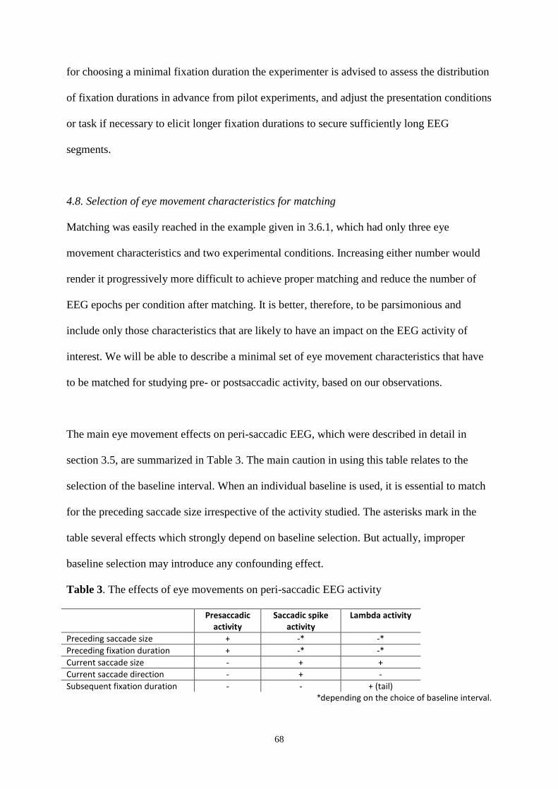
68

for choosing a minimal fixation duration the experimenter is advised to assess the distribution

of fixation durations in advance from pilot experiments, and adjust the presentation conditions

or task if necessary to elicit longer fixation durations to secure sufficiently long EEG

segments.

4.8. Selection of eye movement characteristics for matching

Matching was easily reached in the example given in 3.6.1, which had only three eye

movement characteristics and two experimental conditions. Increasing either number would

render it progressively more difficult to achieve proper matching and reduce the number of

EEG epochs per condition after matching. It is better, therefore, to be parsimonious and

include only those characteristics that are likely to have an impact on the EEG activity of

interest. We will be able to describe a minimal set of eye movement characteristics that have

to be matched for studying pre- or postsaccadic activity, based on our observations.

The main eye movement effects on peri-saccadic EEG, which were described in detail in

section 3.5, are summarized in Table 3. The main caution in using this table relates to the

selection of the baseline interval. When an individual baseline is used, it is essential to match

for the preceding saccade size irrespective of the activity studied. The asterisks mark in the

table several effects which strongly depend on baseline selection. But actually, improper

baseline selection may introduce any confounding effect.

Table 3. The effects of eye movements on peri-saccadic EEG activity

Presaccadic activity

Saccadic spike activity

Lambda activity

Preceding saccade size + -* -*

Preceding fixation duration + -* -*

Current saccade size - + +

Current saccade direction - + -

Subsequent fixation duration - - + (tail) *depending on the choice of baseline interval.

69

In sum, in order to study presaccadic activity the experimental conditions have to be matched

for the duration of preceding fixation as well as for the size and direction of the preceding

saccade. To study postsaccadic activity the experimental conditions have to be matched for

size and direction of the current saccade as well as for the duration of subsequent fixation.

The duration of the preceding fixation should be equal between conditions, if the baseline is

selected in the presaccadic or early postsaccadic interval. As we have seen above, it is

preferable to time-lock epochs to saccade onset when presaccadic activity is being studied and

to fixation onset when postsaccadic activity is being studied. Fig. 15 shows a flowchart to

assist decision making during combined EEG-eye movement analysis.

4.9. Merits of frequency vs. time domain analysis

Traditionally, evoked potentials time-locked to the saccade or fixation onsets have been the

main tool of co-registration research. However, the frequency components of the saccade-

related activity are also of interest, because they may coincide and even be confused with the

brain rhythms reflected in the perceptual and cognitive processes under study. A striking

example of such confusion was demonstrated in the study of microsaccades: concentration of

saccadic spike activity about 300 ms after presentation of a visual stimulus may be mistaken

for an increase in gamma activity due to perceptual processing, because the microsaccade rate

usually increases in this interval (Yuval-Greenberg, Tomer, Keren, Nelken, & Deouell, 2008).

In addition, lambda activity evoked by microsaccades increases the spectral power in the

alpha and theta band. The power increase is followed by several cycles of alpha oscillations

(Dimigen et al., 2009). These may interfere with ongoing alpha activity of cognitive origin.

These observations can be extended to saccades of all sizes because microsaccades and

70

saccades constitute a continuum in terms of physical characteristics and generation

mechanisms (Martinez-Conde, Macknik, Troncoso, & Hubel, 2009).

The filtered evoked potentials and the data in the time-frequency domain are complementary

(see chapter 2 in Cohen (2014) for discussion). On the one hand, evoked potentials have

excellent temporal resolution. Moreover, the extensive literature collected over 70 years of

research has allowed researchers to link the components of evoked potentials to perceptual

and cognitive processes and brain structures. On the other hand, reliable estimation of evoked

potentials is possible only after averaging of many trials. In the averaging, task-relevant

information may be lost (Alexander et al., 2013; Alexander et al., 2015). In contrast, the time-

frequency analysis can reliably be done on single trials, which allows to study how

experimental stimulation modulates ongoing brain activity. Moreover, in contrast to evoked

potentials, of which the origin is often uncertain or consists of a mixture of sources, time-

frequency analysis reveals oscillatory brain activity, of which the mechanisms and generators

are relatively well-understood from animal and in-vitro experiments. Furthermore, synchrony

between oscillations allows evaluation of connectivity between brain areas. The drawback is

that time-frequency decomposition reduces the temporal resolution of the analysis. Even

though to some degree this reduction can be controlled by the parameters of the

decomposition, in general, temporal resolution remains an issue in particular for the lower

frequencies.

The phase of an EEG signal may be of considerable interest in the study of saccade-related

activity in free viewing, because phase is affected by both visual and oculomotor processes at

fixation onset. For example, in free viewing of natural scenes the visually evoked responses

superimpose on the ongoing activity and change its phase (Ossandón et al., 2010). But even in

71

complete darkness, i.e., without visual input, the fixation onset is accompanied by phase

resetting in a wide frequency range of oscillations recorded from monkey V1 (Rajkai et al.,

2008). In scalp-recorded EEG, phase resetting is manifested in the ITC increase at the lambda

latency over the occipital areas (Fig. 3B). Saccade-related phase changes may have the

function of synchronizing brain areas, in order to collectively bring them into an optimal state

for processing of visual information (Jutras & Buffalo, 2010).

5. Conclusion

Co-registration of EEG and eye movements is a valuable technique for investigating the time

course of perceptual and cognitive processes in unconstrained visual behavior. But it does

engender a set of specific methodological problems that are due to the systematic effects of

sequential eye movements on each other’s EEG. These effects could be confused with effects

of experimental conditions. We illustrated the diversity of these distortions. Our proposed

solution consists in matching the relevant eye movement characteristics across experimental

conditions. Matching could be done selectively, aided by the catalogue of distortions we

identified. We believe that inserting this simple and intuitive step into the analysis procedure

makes it possible to widely apply co-registration of EEG and eye movement in various

domains of cognitive neuroscience.

Acknowledgements

The authors were supported by an Odysseus grant from the Flemish Organization for Science

(FWO). We thank Chie Nakatani, Peter Jurica, and Gijs Plomp for help in experimentation

and initial data processing and David Alexander for valuable suggestions.

72

References

Aks, D. J., Zelinsky, G. J., & Sprott, J. C. (2002). Memory across eye-movements: 1/f dynamic in

visual search. Nonlinear Dynamics, Psychology, and Life Sciences, 6(1), 1-25.

Alexander, D. M., Jurica, P., Trengove, C., Nikolaev, A. R., Gepshtein, S., Zvyagintsev, M., et al.

(2013). Traveling waves and trial averaging: the nature of single-trial and averaged brain

responses in large-scale cortical signals. Neuroimage, 73, 95-112.

Alexander, D. M., Trengove, C., & van Leeuwen, C. (2015). Donders is dead: cortical traveling

waves and the limits of mental chronometry in cognitive neuroscience. Cognitive Processing,

16(4), 365-375.

Alexander, D. M., Trengove, C., Wright, J. J., Boord, P. R., & Gordon, E. (2006). Measurement of

phase gradients in the EEG. Journal of Neuroscience Methods, 156(1-2), 111-128.

Becker, W., Hoehne, O., Iwase, K., & Kornhuber, H. H. (1973). Cerebral and ocular muscle

potentials preceding voluntary eye movements in man. Electroencephalography and Clinical

Neurophysiology. Supplement, 33, 99–104.

Belopolsky, A. V., Kramer, A. F., & Theeuwes, J. (2008). The role of awareness in processing of

oculomotor capture: evidence from event-related potentials. Journal of Cognitive

Neuroscience, 20(12), 2285-2297.

Billings, R. J. (1989a). The origin of the initial negative component of the averaged lambda potential

recorded from midline electrodes. Electroencephalography and Clinical Neurophysiology,

72(2), 114-117.

Billings, R. J. (1989b). The origin of the occipital lambda wave in man. Electroencephalography and

Clinical Neurophysiology, 72(2), 95-113.

Boylan, C., & Doig, H. R. (1989). Effect of saccade size on presaccadic spike potential amplitude.

Investigative Ophthalmology and Visual Science, 30(12), 2521-2527.

73

Brouwer, A. M., Reuderink, B., Vincent, J., van Gerven, M. A., & van Erp, J. B. (2013).

Distinguishing between target and nontarget fixations in a visual search task using fixation-

related potentials. Journal of vision, 13(3), 17.

Carpenter, R. H. S. (1988). Movements of the eyes (2nd ed.). London: Pion Press.

Castelhano, M. S., Mack, M. L., & Henderson, J. M. (2009). Viewing task influences eye movement

control during active scene perception. Journal of vision, 9(3), 6 1-15.

Cohen, J. (1988). Statistical Power Analysis for the Behavioral Sciences (2nd ed.). Hillsdale, NJ:

Lawrence Erlbaum Associates.

Cohen, M. (2014). Analyzing neural time series data. Cambridge, Massachusetts MIT Press.

Collewijn, H., van der Steen, J., & Steinman, R. M. (1985). Human eye movements associated with

blinks and prolonged eyelid closure. Journal of Neurophysiology, 54(1), 11-27.

Csibra, G., Johnson, M. H., & Tucker, L. A. (1997). Attention and oculomotor control: a high-density

ERP study of the gap effect. Neuropsychologia, 35(6), 855-865.

Dandekar, S., Ding, J., Privitera, C., Carney, T., & Klein, S. A. (2012). The fixation and saccade P3.

PLoS One, 7(11), e48761.

Dandekar, S., Privitera, C., Carney, T., & Klein, S. A. (2012). Neural saccadic response estimation

during natural viewing. Journal of Neurophysiology, 107(6), 1776-1790.

Delorme, A., & Makeig, S. (2004). EEGLAB: an open source toolbox for analysis of single-trial EEG

dynamics including independent component analysis. Journal of Neuroscience Methods,

134(1), 9-21.

Devillez, H., Guyader, N., & Guerin-Dugue, A. (2015). An eye fixation-related potentials analysis of

the P300 potential for fixations onto a target object when exploring natural scenes. Journal of

vision, 15(13), 20.

Dias, J. C., Sajda, P., Dmochowski, J. P., & Parra, L. C. (2013). EEG precursors of detected and

missed targets during free-viewing search. Journal of vision, 13(13), 13.

74

Dien, J. (1998). Issues in the application of the average reference: Review, critiques, and

recommendations. Behavior Research Methods Instruments & Computers, 30(1), 34-43.

Dimigen, O., Sommer, W., Hohlfeld, A., Jacobs, A. M., & Kliegl, R. (2011). Coregistration of eye

movements and EEG in natural reading: analyses and review. Journal of Experimental

Psychology: General, 140(4), 552-572.

Dimigen, O., Valsecchi, M., Sommer, W., & Kliegl, R. (2009). Human microsaccade-related visual

brain responses. Journal of Neuroscience, 29(39), 12321-12331.

Evans, C. C. (1953). Spontaneous excitation of the visual cortex and association areas; lambda

waves. Electroencephalography and Clinical Neurophysiology, 5(1), 69-74.

Findlay, J. M., & Gilchrist, I. D. (2003). Active vision. New York: Oxford University Press.

Fischer, T., Graupner, S. T., Velichkovsky, B. M., & Pannasch, S. (2013). Attentional dynamics

during free picture viewing: Evidence from oculomotor behavior and electrocortical activity.

Frontiers in systems neuroscience, 7, 17.

Fourment, A., Calvet, J., & Bancaud, J. (1976). Electrocorticography of waves associated with eye

movements in man during wakefulness. Electroencephalography and Clinical

Neurophysiology, 40(5), 457-469.

Fudali-Czyz, A., Francuz, P., & Augustynowicz, P. (2014). Determinants of attentive blank stares.

An EFRP study. Consciousness and Cognition, 29, 1-9.

Fuller, J. H. (1992). Head movement propensity. Experimental Brain Research, 92(1), 152-164.

Gaarder, K., Krauskopf, J., Graf, V., Kropfl, W., & Armington, J. C. (1964). Averaged brain activity

following saccadic eye movement. Science, 146, 1481-1483.

Gastaut, Y. (1951). [A little-known electroencephalographic sign: occipital points occuring during

opening of the eyes.]. Revue Neurologique, 84(6), 635-640.

Gratton, G., Coles, M. G., & Donchin, E. (1983). A new method for off-line removal of ocular

artifact. Electroencephalography and Clinical Neurophysiology, 55(4), 468-484.

75

Graupner, S. T., Velichkovsky, B. M., Pannasch, S., & Marx, J. (2007). Surprise, surprise: two

distinct components in the visually evoked distractor effect. Psychophysiology, 44(2), 251-

261.

Guitton, D., & Volle, M. (1987). Gaze control in humans: eye-head coordination during orienting

movements to targets within and beyond the oculomotor range. Journal of Neurophysiology,

58(3), 427-459.

Gutteling, T. P., van Ettinger-Veenstra, H. M., Kenemans, J. L., & Neggers, S. F. (2010). Lateralized

frontal eye field activity precedes occipital activity shortly before saccades: evidence for

cortico-cortical feedback as a mechanism underlying covert attention shifts. Journal of

Cognitive Neuroscience, 22(9), 1931-1943.

Henderson, J. M., & Hollingworth, A. (1999). High-level scene perception. Annual Review of

Psychology, 50, 243-271.

Henderson, J. M., Weeks, P. A., & Hollingworth, A. (1999). The effects of semantic consistency on

eye movements during complex scene viewing. Journal of Experimental Psychology: Human

Perception and Performance, 25(1), 210-228.

Hoffman, J. E., & Subramaniam, B. (1995). The role of visual attention in saccadic eye movements.

Perception and Psychophysics, 57(6), 787-795.

Hutzler, F., Braun, M., Vo, M. L., Engl, V., Hofmann, M., Dambacher, M., et al. (2007). Welcome to

the real world: validating fixation-related brain potentials for ecologically valid settings.

Brain Research, 1172, 124-129.

Ito, J., Maldonado, P., Singer, W., & Grün, S. (2011). Saccade-related modulations of neuronal

excitability support synchrony of visually elicited spikes. Cerebral Cortex, 21(11), 2482-

2497.

76

Jung, T. P., Makeig, S., Humphries, C., Lee, T. W., McKeown, M. J., Iragui, V., et al. (2000).

Removing electroencephalographic artifacts by blind source separation. Psychophysiology,

37(2), 163-178.

Jutras, M. J., & Buffalo, E. A. (2010). Synchronous neural activity and memory formation. Current

Opinion in Neurobiology, 20(2), 150-155.

Kamienkowski, J. E., Ison, M. J., Quiroga, R. Q., & Sigman, M. (2012). Fixation-related potentials in

visual search: a combined EEG and eye tracking study. Journal of vision, 12(7), 4.

Kaunitz, L. N., Kamienkowski, J. E., Varatharajah, A., Sigman, M., Quiroga, R. Q., & Ison, M. J.

(2014). Looking for a face in the crowd: fixation-related potentials in an eye-movement visual

search task. Neuroimage, 89, 297-305.

Kazai, K., & Yagi, A. (1999). Integrated effect of stimulation at fixation points on EFRP (eye-

fixation related brain potentials). International Journal of Psychophysiology, 32(3), 193-203.

Kazai, K., & Yagi, A. (2003). Comparison between the lambda response of eye-fixation-related

potentials and the P100 component of pattern-reversal visual evoked potentials. Cognitive,

affective & behavioral neuroscience, 3(1), 46-56.

Keren, A. S., Yuval-Greenberg, S., & Deouell, L. Y. (2010). Saccadic spike potentials in gamma-

band EEG: characterization, detection and suppression. Neuroimage, 49(3), 2248-2263.

Klimesch, W., Sauseng, P., & Hanslmayr, S. (2007). EEG alpha oscillations: the inhibition-timing

hypothesis. Brain Research. Brain Research Reviews, 53(1), 63-88.

Körner, C., Braunstein, V., Stangl, M., Schlogl, A., Neuper, C., & Ischebeck, A. (2014). Sequential

effects in continued visual search: using fixation-related potentials to compare distractor

processing before and after target detection. Psychophysiology, 51(4), 385-395.

Körner, C., & Gilchrist, I. D. (2007). Finding a new target in an old display: evidence for a memory

recency effect in visual search. Psychon Bull Rev, 14(5), 846-851.

77

Kovalenko, L. Y., & Busch, N. A. (2016). Probing the dynamics of perisaccadic vision with EEG.

Neuropsychologia, 85, 337-348.

Krebs, R. M., Boehler, C. N., Zhang, H. H., Schoenfeld, M. A., & Woldorff, M. G. (2012).

Electrophysiological recordings in humans reveal reduced location-specific attentional-shift

activity prior to recentering saccades. Journal of Neurophysiology, 107(5), 1393-1402.

Kurtzberg, D., & Vaughan, H. G., Jr. (1982). Topographic analysis of human cortical potentials

preceding self-initiated and visually triggered saccades. Brain Research, 243(1), 1-9.

Lee, E. C., Woo, J. C., Kim, J. H., Whang, M., & Park, K. R. (2010). A brain-computer interface

method combined with eye tracking for 3D interaction. Journal of Neuroscience Methods,

190(2), 289-298.

Leigh, R. J., & Zee, D. S. (2006). The neurology of eye movements (4th ed.). New York: Oxford

University Press.

Lins, O. G., Picton, T. W., Berg, P., & Scherg, M. (1993). Ocular artifacts in recording EEGs and

event-related potentials. II: Source dipoles and source components. Brain Topography, 6(1),

65-78.

Loftus, G. R. (1985). Picture perception: effects of luminance on available information and

information-extraction rate. Journal of Experimental Psychology: General, 114(3), 342-356.

Loftus, G. R., Kaufman, L., Nishimoto, T., & Ruthruff, E. (1992). Effects of visual degradation on

eye-fixation durations, perceptual processing, and long-term visual memory. In K. Rayner

(Ed.), Eye movements and visual cognition: Scene perception and reading (pp. 203-226).

New York: Springer.

Luck, S. J. (2005). An Introduction to the Event-Related Potential Technique. Cambridge, MA: MIT

Press.

78

Ma, J., Bayram, S., Tao, P., & Svetnik, V. (2011). High-throughput ocular artifact reduction in

multichannel electroencephalography (EEG) using component subspace projection. Journal of

Neuroscience Methods, 196(1), 131-140.

Martinez-Conde, S., Macknik, S. L., Troncoso, X. G., & Hubel, D. H. (2009). Microsaccades: a

neurophysiological analysis. Trends in Neurosciences, 32(9), 463-475.

Meghanathan, R. N., van Leeuwen, C., & Nikolaev, A. R. (2015). Fixation duration surpasses pupil

size as a measure of memory load in free viewing. Frontiers in human neuroscience, 8, 1063.

Miller, G. A., & Chapman, J. P. (2001). Misunderstanding analysis of covariance. Journal of

Abnormal Psychology, 110(1), 40-48.

Moster, M. L., & Goldberg, G. (1990). Topography of scalp potentials preceding self-initiated

saccades. Neurology, 40(4), 644-648.

Nikolaev, A. R., Jurica, P., Nakatani, C., Plomp, G., & van Leeuwen, C. (2013). Visual encoding and

fixation target selection in free viewing: presaccadic brain potentials. Frontiers in systems

neuroscience, 7, 26.

Nikolaev, A. R., Nakatani, C., Plomp, G., Jurica, P., & van Leeuwen, C. (2011). Eye fixation-related

potentials in free viewing identify encoding failures in change detection. Neuroimage, 56(3),

1598-1607.

Nikolaev, A. R., Pannasch, S., Ito, J., & Belopolsky, A. V. (2014). Eye movement-related brain

activity during perceptual and cognitive processing. Frontiers in systems neuroscience, 8, 62.

Onton, J., Westerfield, M., Townsend, J., & Makeig, S. (2006). Imaging human EEG dynamics using

independent component analysis. Neuroscience and Biobehavioral Reviews, 30(6), 808-822.

Ossandón, J. P., Helo, A. V., Montefusco-Siegmund, R., & Maldonado, P. E. (2010). Superposition

model predicts EEG occipital activity during free viewing of natural scenes. Journal of

Neuroscience, 30(13), 4787-4795.

79

Parks, N. A., & Corballis, P. M. (2008). Electrophysiological correlates of presaccadic remapping in

humans. Psychophysiology, 45(5), 776-783.

Peterson, M. A., & Gibson, B. S. (1991). Directing spatial attention within an object: altering the

functional equivalence of shape descriptions. Journal of Experimental Psychology: Human

Perception and Performance, 17(1), 170-182.

Plöchl, M., Ossandón, J. P., & König, P. (2012). Combining EEG and eye tracking: identification,

characterization, and correction of eye movement artifacts in electroencephalographic data.

Frontiers in human neuroscience, 6, 278.

Rajkai, C., Lakatos, P., Chen, C. M., Pincze, Z., Karmos, G., & Schroeder, C. E. (2008). Transient

cortical excitation at the onset of visual fixation. Cerebral Cortex, 18(1), 200-209.

Rama, P., & Baccino, T. (2010). Eye fixation-related potentials (EFRPs) during object identification.

Visual Neuroscience, 27(5-6), 187-192.

Rensink, R., O'Regan, J., & Clark, J. (1997). To see or not to see: the need for attention to perceive

changes in scenes. Psychological science, 8, 368-373.

Richards, J. E. (2000). Localizing the development of covert attention in infants with scalp event-

related potentials. Developmental Psychology, 36(1), 91-108.

Richards, J. E. (2003). Cortical sources of event-related potentials in the prosaccade and antisaccade

task. Psychophysiology, 40(6), 878-894.

Riemslag, F. C., Van der Heijde, G. L., Van Dongen, M. M., & Ottenhoff, F. (1988). On the origin of

the presaccadic spike potential. Electroencephalography and Clinical Neurophysiology,

70(4), 281-287.

Riggs, L. A., Merton, P. A., & Morton, H. B. (1974). Suppression of visual phosphenes during

saccadic eye-movements. Vision Research, 14(10), 997-1011.

80

Romero, S., Mananas, M. A., & Barbanoj, M. J. (2008). A comparative study of automatic techniques

for ocular artifact reduction in spontaneous EEG signals based on clinical target variables: a

simulation case. Computers in Biology and Medicine, 38(3), 348-360.

Rosenbaum, P. R. (2005). An exact distribution-free test comparing two multivariate distributions

based on adjacency. Journal of the Royal Statistical Society Series B-Statistical Methodology,

67, 515-530.

Simola, J., Le Fevre, K., Torniainen, J., & Baccino, T. (2015). Affective processing in natural scene

viewing: valence and arousal interactions in eye-fixation-related potentials. Neuroimage, 106,

21-33.

Simola, J., Torniainen, J., Moisala, M., Kivikangas, M., & Krause, C. M. (2013). Eye movement

related brain responses to emotional scenes during free viewing. Frontiers in systems

neuroscience, 7, 41.

Stahl, J. S. (1999). Amplitude of human head movements associated with horizontal saccades.

Experimental Brain Research, 126(1), 41-54.

Storey, J. D. (2002). A direct approach to false discovery rates. Journal of the Royal Statistical

Society Series B-Statistical Methodology, 64, 479-498.

Tallon-Baudry, C., Bertrand, O., Delpuech, C., & Pernier, J. (1996). Stimulus specificity of phase-

locked and non-phase-locked 40 Hz visual responses in human. Journal of Neuroscience,

16(13), 4240-4249.

Tatler, B. W., & Vincent, B. T. (2008). Systematic tendencies in scene viewing. Journal of Eye

Movement Research, 2(2).

Thickbroom, G. W., Knezevic, W., Carroll, W. M., & Mastaglia, F. L. (1991). Saccade onset and

offset lambda waves: relation to pattern movement visually evoked potentials. Brain

Research, 551(1-2), 150-156.

81

Thickbroom, G. W., & Mastaglia, F. L. (1986). Presaccadic spike potential. Relation to eye

movement direction. Electroencephalography and Clinical Neurophysiology, 64(3), 211-214.

Tremblay, A., & Newman, A. J. (2015). Modeling nonlinear relationships in ERP data using mixed-

effects regression with R examples. Psychophysiology, 52(1), 124-139.

Unema, P. J. A., Pannasch, S., Joos, M., & Velichkovsky, B. M. (2005). Time course of information

processing during scene perception: The relationship between saccade amplitude and fixation

duration. Visual Cognition, 12(3), 473-494.

Wauschkuhn, B., Verleger, R., Wascher, E., Klostermann, W., Burk, M., Heide, W., et al. (1998).

Lateralized human cortical activity for shifting visuospatial attention and initiating saccades.

Journal of Neurophysiology, 80(6), 2900-2910.

Wellek, S. (2010). Testing statistical hypotheses of equivalence and noninferiority (2nd ed.):

Chapman and Hall/CRC.

Wildt, A. R., & Ahtola, O. T. (1978). Analysis of covariance. Beverly Hills, CA: Sage.

Wood, S. N. (2006). Generalized additive models. New York: Chapman & Hall/CRC.

Yagi, A. (1979). Saccade size and lambda complex in man. Physiological Psychology, 7, 370-376.

Yuval-Greenberg, S., Tomer, O., Keren, A. S., Nelken, I., & Deouell, L. Y. (2008). Transient induced

gamma-band response in EEG as a manifestation of miniature saccades. Neuron, 58(3), 429-

441.

Zander, T. O., Gaertner, M., Kothe, C., & Vilimek, R. (2011). Combining eye gaze input with a

brain-computer interface for touchless human-computer interaction. International Journal of

Human-Computer Interaction, 27(1), 38-51.

82

Figure captions

Figure 1. Examples of stimuli used in two free-viewing experiments. A. An example of a

natural scene used in the encoding stage of the change blindness task for the “CB dataset”. B.

An example of an array containing Ts among Ls used in the multiple-target search stage of

the change detection task for the “VS dataset”.

Figure 2. Eye movement characteristics in two datasets: change blindness (CB) and

visual search (VS). A. Saccade duration. B. Fixation duration. C. Saccade direction.

Figure 3. CB dataset: main EEG activity around a saccade averaged across 15

participants for 13 scalp electrodes. A. Saccade-related potentials (red curves, left Y-axis)

superimposed on the time-frequency plots of EEG log-power time-locked to saccade onset. B.

The time-frequency plots of inter-trial coherence (ITC) relative to saccade onset.

Figure 4. VS dataset: main EEG activity around saccades averaged across 21

participants. Activity time-locked to saccade onset is in A-C; activity time-locked to fixation

onset is in D-F. A. Evoked potential voltage maps. B. Saccade-related potential (red curve,

left Y-axis) superimposed on time-frequency plot of EEG log-power (the scale is indicated by

numbers on the contour lines) for activity averaged across seven electrodes over the left

occipital area (OL). C. Maps of log-power distribution at specified time points and

frequencies. D. Evoked potential voltage maps E. Saccade-related potential (red curve, left Y-

axis) superimposed on time-frequency plot of EEG log-power (the scale is indicated by

numbers on the contour lines) for activity averaged across seven electrodes over OL. F. Maps

of log-power distribution at specified time points and frequencies. In A, C, D, F the left map

83

shows the mean activity in the presaccadic interval; the central map is taken at the maximum

of the saccadic spike activity; the right map is taken at the maximum of the lambda activity.

Figure 5. CB dataset: Segmentation relative to saccade vs. fixation onsets: power. A. EEG

log-power at 5 Hz time-locked to saccade and fixation onsets after shifting in time the

fixation-locked activity, in order to compensate for saccade duration. B. The same at 35 Hz.

The inset shows EEG log-power at 35 Hz time-locked to saccade and fixation onsets before

shifting in time. C. Intervals of significant difference between EEG power time-locked to

saccade and fixation onsets after the shift.

Figure 6. CB dataset: Segmentation relative to saccade vs. fixation onsets: ITC. A. ITC at

5 Hz time-locked to saccade and fixation onsets after shifting the fixation-locked activity. B.

The same at 35 Hz. C. Intervals of significant difference between ITC time-locked to saccade

and fixation onsets after the shift.

Figure 7. CB dataset: Time-locking relative to saccade vs. fixation onsets. A. EEG log-

power (left Y axis) and ITC (right Y axis) time-locked to saccade onset for three EEG

frequencies in electrode O1. B. The same for activity time-locked to fixation onset. C. Peak

latency of power and ITC time-locked to fixation onset at 35 Hz in four brain regions. Error

bars indicate standard errors of the means across 15 participants.

Figure 8. Possible locations of baseline interval. Rectangular frames designate trials with

duration of several seconds and containing multiple fixations (=saccade-related epochs). Solid

bars designate saccade-related epochs. Pink bars designate possible baseline locations. A. A

common baseline. B. A local baseline. C. An individual baseline.

84

Figure 9. CB dataset: Effect of preceding saccade size on EEG. A. EEG log-power at 10

Hz in electrode O1, time-locked to saccade onset, in three saccade size bins with equal

numbers of epochs for baseline -300-250 ms. C. Intervals of significant difference between

bins in A. B-D. The same for baseline -100-50 ms. Pink bars designate baseline locations.

Figure 10. CB dataset: Effect of preceding fixation duration on EEG. A. EEG log-power

at 10 Hz in electrode O1, time-locked to saccade onset in three fixation duration bins with

equal numbers of epochs for baseline -300-250 ms. D. Intervals of significant difference

between bins in A. B-E. The same for baseline -100-50 ms. C. EEG log-power at 10 Hz in

electrode O1, time-locked to fixation onset in three fixation duration bins with equal numbers

of epochs for baseline 0-20 ms. F. Intervals of significant difference between bins in C. Pink

bars designate baseline locations.

Figure 11. CB dataset: Effect of saccade size on EEG. Activity time-locked to saccade

onset is in A-F; activity time locked to fixation onset is in H-M. Error bars indicate standard

errors of the means across 15 participants. A. Saccade-related potential time-locked to

saccade onset in three saccade size bins with equal number of epochs for electrode Fz. B. The

same for electrode O1. C. Peak-to-peak amplitude of the saccadic spike potential (“SP”) and

difference in amplitude between lambda and negative saccadic spike peaks (“Lambda”) for

three saccade size bins. D. EEG log-power at 35 Hz time-locked to saccade onset in three

saccade size bins with equal numbers of epochs for electrode Fz. E. The same for 10 Hz and

electrode O1. F. Intervals of significant difference between three bins. G. Difference in

saccadic spike and lambda power between the third and first bin at each frequency in the 5-45

Hz range. H. Saccade-related potential time-locked to fixation onset in three saccade size bins

85

with equal number of epochs for electrode Fz. I. The same for electrode O1. J. The peak-to-

peak amplitude for the saccadic spike potential and difference in amplitude between lambda

and negative saccadic spike peaks for three saccade size bins. K. EEG log-power at 35 Hz

time-locked to fixation onset in three saccade size bins with equal numbers of epochs for

electrode Fz. L. The same for 10 Hz and electrode O1. M. Intervals of significant difference

between three bins.

Figure 12. CB dataset: Effect of saccade direction on EEG. A. Saccade-related potential

time-locked to saccade onset in the left frontal electrode F3 for four saccade directions. B.

The same for the right frontal electrode F4. C. The same for electrode O1. D. EEG log-power

at 35 Hz time-locked to saccade onset in the left frontal electrode F3 for four saccade

directions. E. The same for the right frontal electrode F4. F. The same for electrode O1. G.

Saccade duration and mean log-power at 35 Hz of saccadic spike activity in left (F3) and right

(F4) frontal electrodes for four saccade directions.

Figure 13. CB dataset: Effect of subsequent fixation duration on EEG. A. Saccade-related

potential time-locked to fixation onset in three subsequent fixation duration bins with equal

numbers of epochs for electrode Fz. B. The same for electrode O1. C. EEG log-power at 10

Hz time-locked to fixation onset in three subsequent fixation duration bins with equal

numbers of epochs for electrode Fz. D. The same for 10 Hz and electrode O1. E. The intervals

of significant difference between three bins.

Figure 14. Matching of eye movement characteristics. A. Schematic illustration of

matching eye movement parameters based on Mahalanobis distance. Eye movement

characteristics for two hypothetical conditions are shown as data points within a large circle.

86

Distance of a data point from the center represents saccade size. Size of the data point marker

represents fixation duration. The angular position along the circle indicates saccade direction.

Mahalanobis distance of each point from the reference distribution is depicted in the color of

each data point. Data points above the cutoff Mahalanobis distance are crossed out indicating

elimination in the matching procedure. B. Histograms of distributions of three eye movement

characteristics in conditions of central and marginal interest (see text for explanation) for one

participant before and after the matching procedure.

Figure 15. A flowchart for the combined EEG-eye movement analysis.

A

B

Figure1

0 10 20 30 40 50 60 70 80

00

*10

1

2

2

3

3

4

4

6

0

*10

2

3

4

6N

of

sa

cca

de

s.

CB

da

tase

t

0

*10

2

3

4

N o

f sa

cca

de

s.

CB

da

tase

tN

of

fixa

tio

ns.

CB

da

tase

t

0

1

2

3

*104

*104

*104

4

N o

f sa

cca

de

s.

VS

da

tase

t

0

0.4

0.8

1.2

1.6

2.0

N o

f sa

cca

de

s.

VS

da

tase

tN

of

fixa

tio

ns.

VS

da

tase

t

Saccade duration, ms

Fixation duration, ms

Direction from the horizontal, deg

0 100 200 300 400 500 600 700 800 900 1000

0 40 80 120 160 200 240 280 320 360

CB dataset

VS dataset

A

C

B

Figure2

Figure3Click here to download high resolution image

Figure4Click here to download high resolution image

Po

we

rP

ow

er

0.0

0.4

0.8

B

O1 O2

C3 C4Cz

F3 F4Fz

P3 P4Pz

T5 T6

-0.2

0.0

0.2

A

O1 O2

C3 C4Cz

F3 F4Fz

P3 P4Pz

T5T6

Fz

Sac nsetcade o

Fix nsetation o

Fre

qu

en

cy,

Hz

6

10

17

28

45

C

O1 O2

C3 C4Cz

F3 F4Fz

P3 P4Pz

T5 T6

-300 0 300

-300 0 300

-300 0 300

current

saccade

saccade onset

preceding

saccade

preceding

fixation

fixation onset

subsequent

fixation

Figure5

C

B

ITC

ITC

A

O1 O2

C3 C4Cz

F3 F4Fz

P3 P4Pz

T5 T6

-300 0 300

Fre

qu

en

cy,

Hz

6

10

17

28

45

O1 O2

C3 C4Cz

F3 F4Fz

P3 P4Pz

T5 T6

0.0

0.2

0.4

-300 0 300

0.0

0.2

0.4O1 O2

C3 C4Cz

F3 F4Fz

P3 P4Pz

T5 T6

-300 0 300

current

saccade

saccade onset

preceding

saccade

preceding

fixation

fixation onset

subsequent

fixation

Sac nsetcade o

Fix nsetation o

Figure6

A

C

B

-0.2

0.0

0.2

0.0

0.1

0.2

0.35 Hz

-0.2

0.0

0.2

0.4

0.0

0.2

10 Hz

ITC

ITC

ITC

Fixation onsetSaccade onset

-0.2

0.0

0.2

0.0

0.1

0.2

0.35 Hz

-0.2

0.0

0.2

0.0

0.2

10 Hz

0.0

0.2

0.4

0.0

0.1

0.2

35 Hz

0.0

0.2

0.4

0.6

0.0

0.2

0.435 Hz

Po

we

rP

ow

er

Po

we

r

Frontal

Central

Parietal

Occipital

0 0300 300-300 -300

Time from saccade, ms Time from fixation, ms

-20 -10 0

Peak latency from fixation, ms

10

ITC

Power

Lag

current

saccade

saccade onset

preceding

saccade

preceding

fixation

fixation onset

subsequent

fixation

Figure7

A

C

B

trial

onset

a saccade-related epoch

a t r i a l

individual baseline

local baseline

common

baseline

Figure8

A B

5

6

8

10

13

17

22

28

35

45

Pow

er

Time from saccade, ms Time from saccade, ms

-200 -200-100 -1000 0100 100200 200300 300-300 -300

Fre

quency, H

z

C D

0.0

0.4

0.8

-0.4

0.0

0.4

current

saccade

saccade onset

preceding

saccade

preceding

fixation

fixation onset

subsequent

fixation

preceding

saccade size

small

med

large

Figure9

Po

we

r

A C

D F

B

-0.5

0.0

0.5

0.0

0.4

0.8

E

0.0

0.4

current

saccade

saccade onset

preceding

saccade

preceding

fixation

fixation onset

subsequent

fixation

preceding sfixation

short

med

long

Time from saccade, ms Time from saccade, ms Time from fixation, ms

-200 -200 -200-100 -100 -1000 0 0100 100 100200 200 200300 300 300-300 -300 -300

5

6

8

10

13

17

22

28

35

45

Fre

qu

en

cy,

Hz

Figure10

A

Pow

er

Pow

er

Time from saccade, ms

-300 -200 -100 0 100 200 300

Time from saccade, ms

-300 -200 -100 0 100 200 300

B

ED F

G

H I J

K L M

C

O1

10 Hz

-0.4

0.0

0.4

0.8

Time from saccade, ms

-300 -200 -100 0 100 200 300

O1

5

6

8

10

13

17

22

28

35

45

Fre

qu

en

cy,

Hz

Frequency, Hz

Am

plitu

de, µ

VA

mplitu

de, µ

V

-4

0

4O1

Fz

0

4

Fz

35 Hz

0.0

0.4

0.8

-4

0

4O1

-2

0

2

4Fz

Time from fixation, ms

-300 -200 -100 0 100 200 300

0.0

0.4

0.8Fz

Time from fixation, ms

-300 -200 -100 0 100 200 300

0.0

0.4

O1

Time from fixation, ms

-300 -200 -100 0 100 200 300

O1

Fre

qu

en

cy,

Hz

5

6

8

10

13

17

22

28

35

45

current

saccade

saccade onset

preceding

saccade

preceding

fixation

fixation onset

subsequent

fixation

current

saccade

saccade onset

preceding

saccade

preceding

fixation

fixation onset

subsequent

fixation

saccade size

small

med

large

SP

am

plitu

de

, µ

V

La

mb

da

am

plitu

de

, µ

V

Saccade size bins

SP

am

plitu

de

, µ

V

La

mb

da

am

plitu

de

, µ

V

Saccade size bins

1 2 34

6

8

10

7

9

11

13

SPLambda

5 6 8 10 13 17 22 28 35 450.1

0.3

0.5

0.7SPLambda

SPLambda

1 2 34

5

6

7

8

6

8

10

12

Po

we

r d

iff

= b

in3

- b

in1

Figure11

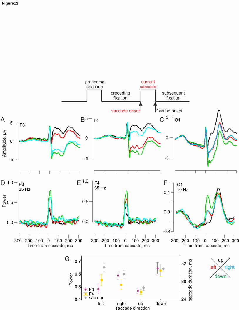
BA

up

rightleft

down

Pow

er

C

D

-5

0

5O1

Am

plitu

de, µ

V

-5

0

5F3

-5

0

5F4

0.0

0.5

1.0F4

35 Hz

0.0

0.5

1.0F3

35 Hz

-0.4

0.0

0.4

O1

10 Hz

E F

G

Pow

er

left up downright

saccade direction

saccade d

ura

tion, m

s

0.1

0.3

0.5

0.7

24

28

32

F3

F4sac dur

current

saccade

saccade onset

preceding

saccade

preceding

fixation

fixation onset

subsequent

fixation

Time from saccade, ms

-300 -200 -100 0 100 200 300

Time from saccade, ms

-300 -200 -100 0 100 200 300

Time from saccade, ms

-300 -200 -100 0 100 200 300

Figure12

A B

C D

Pow

er

s subsequent fixation

short

med

long

-0.2

0.0

0.2

0.4O1

10 Hz

-0.2

0.0

0.2Fz

10 Hz

-2

0

2

4O1

-2

0

2 Fz

Am

plitu

de, µ

V

E

current

saccade

saccade onset

preceding

saccade

preceding

fixation

fixation onset

subsequent

fixation

Time from fixation, ms

-300 -200 -100 0 100 200 300

Time from fixation, ms

-300 -200 -100 0 100 200 300

5

6

8

10

13

17

22

28

35

45

Fz

Time from fixation, ms

-300 -200 -100 0 100 200 300

Fre

quency, H

z

Figure12

0

1

Cutoff

Mahala

nobis

dis

tance

Condition 2

Condition 1

0º

45º

90º

135º

180º

225º

270º

315º

Num

ber

of observ

ations

Before After

A

B

400 800 1200 1600 2000

Fixation duration, ms

2

8

20

40

80

200

90 180 270 360

Saccade direction, deg

20

40

60

80

100

Saccade duration, ms Saccade duration, ms

400 800 1200 1600 2000

Fixation duration, ms

90 180 270 360

Saccade direction, deg

Central

Marginal

10 30 50 70

4

8

20

40

80

10 30 50 70

Figure14

Does the process of

interest involve the

postsaccadic activity?

Segment relative to fixation onset Segment relative to saccade onset

Are experimental

conditions equal in current

saccade size and direction,

preceding and subsequent

fixation duration?

Are experimental

conditions equal in preceding

saccade size and direction,

preceding fixation duration?

Match eye movement

characteristics

Select the baseline interval

Proceed with EEG analysis

yes

yes yes

no

nono

Figure15