University of California, Berkeley

From the SelectedWorks of Jim Pitman

January 2006

Combinatorial Stochastic Processes

ContactAuthor

Start Your OwnSelectedWorks

Notify Meof New Work

Available at: http://works.bepress.com/jim_pitman/1

Combinatorial Stochastic Processes

Jim Pitman

1

2 Jim Pitman

Combinatorial stochastic

processes

Preliminaries

0.0. Preface

This is a collection of expository articles about various topics at the interfacebetween enumerative combinatorics and stochastic processes. These articles ex-pand on a course of lectures given at the Ecole d’Ete de Probabilites de St.Flour in July 2002. The articles are called ’chapters’ and numbered accordingto the order of these chapters in a printed volume to appear in Springer LectureNotes in Mathematics. Each chapter is fairly self-contained, so readers with ad-equate background can start reading any chapter, with occasional consultationof earlier chapters as necessary. Following this Chapter 0, there are 10 chapters,each divided into sections. Most sections conclude with some Exercises. Thosefor which I don’t know solutions are called Problems.

Acknowledgments Much of the research reviewed here was done jointly withDavid Aldous. Much credit is due to him, especially for the big picture of contin-uum approximations to large combinatorial structures. Thanks also to my othercollaborators in this work, especially Jean Bertoin, Michael Camarri, StevenEvans, Sasha Gnedin, Ben Hansen, Jacques Neveu, Mihael Perman, Ravi Sheth,Marc Yor and Jim Young. A preliminary version of these notes was developedin Spring 2002 with the help of a dedicated class of ten graduate students inBerkeley: Noam Berger, David Blei, Rahul Jain, Serban Nacu, Gabor Pete,Lea Popovic, Alan Hammond, Antar Bandyopadhyay, Manjunath Krishnapurand Gregory Miermont. The last four deserve special thanks for their contri-butions as research assistants. Thanks to the many people who have read ver-sions of these notes and made suggestions and corrections, especially DavidAldous, Jean Bertoin, Aubrey Clayton, Shankar Bhamidj, Rui Dong, StevenEvans, Sasha Gnedin, Benedicte Haas, Jean-Francois Le Gall, Neil O’Connell,Mihael Perman, Lea Popovic, Jason Schweinsberg. Special thanks to Marc Yorand Matthias Winkel for their great help in preparing the final version of thesenotes for publication. Thanks also to Jean Picard for his organizational effortsin making arrangements for the St. Flour Summer School. This work was sup-ported in part by NSF Grants DMS-0071448 and DMS-0405779.

3

4 Jim Pitman

0.1. Introduction

The main theme of this course is the study of various combinatorial models ofrandom partitions and random trees, and the asymptotics of these models re-lated to continuous parameter stochastic processes. A basic feature of models forrandom partitions is that the sum of the parts is usually constant. So the sizesof the parts cannot be independent. But the structure of many natural mod-els for random partitions can be reduced by suitable conditioning or scaling toclassical probabilistic results involving sums of independent random variables.Limit models for combinatorially defined random partitions are consequentlyrelated to the two fundamental limit processes of classical probability theory:Brownian motion and Poisson processes. The theory of Brownian motion andrelated stochastic processes has been greatly enriched by the recognition thatsome fundamental properties of these processes are best understood in terms ofhow various random partitions and random trees are embedded in their paths.This has led to rapid developments, particularly in the theory of continuumrandom trees, continuous state branching processes, and Markovian superpro-cesses, which go far beyond the scope of this course. Following is a list of themain topics to be treated:

• models for random combinatorial structures, such as trees, forests, permu-tations, mappings, and partitions;

• probabilistic interpretations of various combinatorial notions e.g. Bell poly-nomials, Stirling numbers, polynomials of binomial type, Lagrange inver-sion;

• Kingman’s theory of exchangeable random partitions and random discretedistributions;

• connections between random combinatorial structures and processes withindependent increments: Poisson-Dirichlet limits;

• random partitions derived from subordinators;• asymptotics of random trees, graphs and mappings related to excursions

of Brownian motion;• continuum random trees embedded in Brownian motion;• Brownian local times and squares of Bessel processes;• various processes of fragmentation and coagulation, including Kingman’s

coalescent, the additive and multiplicative coalescents

Next, an incomplete list and topics of current interest, with inadequate refer-ences. These topics are close to those just listed, and certainly part of the realmof combinatorial stochastic processes, but not treated here:

• probability on trees and networks, as presented in [292];• random integer partitions [159, 104], random Young tableaux, growth of

Young diagrams, connections with representation theory and symmetricfunctions [245, 420, 421, 239];

• longest increasing subsequence of a permutation, connections with randommatrices [28];

0.2. BROWNIAN MOTION AND RELATED PROCESSES 5

• random partitions related to uniformly chosen invertible matrices over afinite field, as studied by Fulman [160];

• random maps, coalescing saddles, singularity analysis, and Airy phenom-ena, [81];

• random planar lattices and integrated superbrownian excursion [94].

The reader of these notes is assumed to be familiar with the basic theoryof probability and stochastic processes, at the level of Billingsley [64] or Dur-rett [122], including continuous time stochastic processes, especially Brownianmotion and Poisson processes. For background on some more specialized top-ics (local times, Bessel processes, excursions, SDE’s) the reader is referred toRevuz-Yor [384]. The rest of this Chapter 0 reviews some basic facts from thisprobabilistic background for ease of later reference. This material is organizedas follows:

0.2. Brownian motion and related processes This section provides someminimal description of the background expected of the reader to followsome of the more advanced sections of the text. This includes the defi-nition and basic properties of Brownian motion B := (Bt, t ≥ 0), and ofsome important processes derived from B by operations of scaling andconditioning. These processes include the Brownian bridge, Brownian me-ander and Brownian excursion. The basic facts of Ito’s excursion theoryfor Brownian motion are also recorded.

0.3. Subordinators This section reviews a few basic facts about increasingLevy processes in general, and some important facts about gamma andstable processes in particular.

0.2. Brownian motion and related processes

Let Sn := X1 + . . .+Xn where the Xi are independent random variables withmean 0 and variance 1, and let St for real t be defined by linear interpolationbetween integer values. According to Donsker’s theorem [64, 65, 122, 384]

(Snt/√n, 0 ≤ t ≤ 1)

d→ (Bt, 0 ≤ t ≤ 1) (0.1)

in the usual sense of convergence in distribution of random elements of C[0, 1],where (Bt, t ≥ 0) is a standard Brownian motion meaning that B is a processwith continuous paths and stationary independent Gaussian increments, with

Btd=√tB1 where B1 is standard Gaussian.

Brownian bridge Assuming now that the Xi are integer valued, some con-ditioned forms of Donsker’s theorem can be presented as follows. Let o(

√n)

denote any sequence of possible values of Sn with o(√n)/√n → 0 as n → ∞.

Then [128]

(Snt/√n, 0 ≤ t ≤ 1 |Sn = o(

√n))

d→ (Bbrt , 0 ≤ t ≤ 1) (0.2)

6 Jim Pitman

where Bbr is the standard Brownian bridge, that is, the centered Gaussian pro-cess obtained by conditioning (Bt, 0 ≤ t ≤ 1) on B1 = 0. Some well knowndescriptions of the distribution of Bbr are [384, Ch. III, Ex (3.10)]

(Bbrt , 0 ≤ t ≤ 1)

d= (Bt − tB1, 0 ≤ t ≤ 1)

d= ((1− t)Bt/(1−t), 0 ≤ t ≤ 1) (0.3)

whered= denotes equality of distributions on the path space C[0, 1], and the

rightmost process is defined to be 0 for t = 1.

Brownian meander and excursion Let T− := infn : Sn < 0. Then asn→∞

(Snt/√n, 0 ≤ t ≤ 1 |T− > n)

d→ (Bmet , 0 ≤ t ≤ 1) (0.4)

where Bme is the standard Brownian meander [205, 71], and as n→∞ throughpossible values of T−

(Snt/√n, 0 ≤ t ≤ 1 |T− = n)

d→ (Bext , 0 ≤ t ≤ 1) (0.5)

where Bext is the standard Brownian excursion [225, 102]. Informally,

Bme d= (B |Bt > 0 for all 0 < t < 1)

Bex d= (B |Bt > 0 for all 0 < t < 1, B1 = 0)

whered= denotes equality in distribution. These definitions of conditioned

Brownian motions have been made rigorous in a number of ways: for instanceby the method of Doob h-transforms [255, 394, 155], and as weak limits as ε ↓ 0of the distribution of B given suitable events Aε, as in [124, 69], for instance

(B |B(0, 1) > −ε) d→ Bme as ε ↓ 0 (0.6)

(Bbr |Bbr(0, 1) > −ε) d→ Bex as ε ↓ 0 (0.7)

where X(s, t) denotes the infimum of a process X over the interval (s, t).

Brownian scaling For a process X := (Xt, t ∈ J) parameterized by an in-terval J , and I = [GI , DI ] a subinterval of J with length λI := DI − GI > 0,we denote by X [I ] or X [GI , DI ] the fragment of X on I , that is the process

X [I ]u := XGI+u (0 ≤ u ≤ λI). (0.8)

We denote by X∗[I ] or X∗[GI , DI ] the standardized fragment of X on I , definedby the Brownian scaling operation

X∗[I ]u :=XGI+uλI

−XGI√λI

( 0 ≤ u ≤ 1). (0.9)

For T > 0 let GT := sups : s ≤ T,Bs = 0 be the last zero of B beforetime T and DT := infs : s > T,Bs = 0 be the first zero of B after time

0.2. BROWNIAN MOTION AND RELATED PROCESSES 7

T . Let |B| := (|Bt|, t ≥ 0), called reflecting Brownian motion. It is well known[211, 98, 384] that for each fixed T > 0, there are the following identities indistribution derived by Brownian scaling:

B∗[0, T ]d= B[0, 1]; B∗[0, GT ]

d= Bbr (0.10)

|B|∗[GT , T ]d= Bme; |B|∗[GT , DT ]

d= Bex. (0.11)

It is also known that Bbr, Bme and Bex can be constructed by various otheroperations on the paths of B, and transformed from one to another by furtheroperations [53].

For 0 < t < ∞ let Bbr,t be a Brownian bridge of length t, which may beregarded as a random element of C[0, t] or of C[0,∞], as convenient:

Bbr,t(s) :=√tBbr((s/t) ∧ 1) (s ≥ 0). (0.12)

Let Bme,t denote a Brownian meander of length t, and Bex,t be a Brownianexcursion of length t, defined similarly to (0.12) with Bme or Bex instead ofBbr.

Brownian excursions and the three-dimensional Bessel process Thefollowing theorem summarizes some important relations between Brownian ex-cursions and a particular time-homogeneous diffusion process R3 on [0,∞),commonly known as the three-dimensional Bessel process BES(3), due to therepresentation

(R3(t), t ≥ 0)d=

√√√√

3∑

i=1

(Bi(t))2, t ≥ 0

(0.13)

where the Bi are three independent standard Brownian motions. It should beunderstood however that this particular representation of R3 is a relativelyunimportant coincidence in distribution. What is more important, and canbe understood entirely in terms of the random walk approximations (0.1) and(0.5) of Brownian motion and Brownian excursion, is that there exists a time-homogeneous diffusion process R3 on [0,∞) with R3(0) = 0, which has thesame self-similarity property as B, meaning invariance under Brownian scal-ing, and which can be characterized in various ways, including (0.13), but mostimportantly as a Doob h-transform of Brownian motion.

Theorem 0.1. For each fixed t > 0, the Brownian excursion Bex,t of length tis the BES(3) bridge from 0 to 0 over time t, meaning that

(Bex,t(s), 0 ≤ s ≤ t) d= (R3(s), 0 ≤ s ≤ t |R3(t) = 0).

Moreover, as t→∞Bex,t d→ R3, (0.14)

and R3 can be characterized in two other ways as follows:

8 Jim Pitman

(i) [303, 436] The process R3 is a Brownian motion on [0,∞) started at 0 andconditioned never to return to 0, as defined by the Doob h-transform, for theharmonic function h(x) = x of Brownian motion on [0,∞), with absorbtion at0. That is, R3 has continuous paths starting at 0, and for each 0 < a < b thestretch of R3 between when it first hits a and first hits b is distributed like Bwith B0 = a conditioned to hit b before 0.(ii) [345]

R3(t) = B(t)− 2B(t) (t ≥ 0) (0.15)

where B is a standard Brownian motion with past minimum process

B(t) := B[0, t] = −R3[t,∞).

Levy’s identity The identity in distribution (0.15) admits numerous varia-tions and conditioned forms [345, 53, 55] by virtue of Levy’s identity of jointdistributions of paths [384]

(B −B,−B)d= (|B|, L) (0.16)

where L := (Lt, t ≥ 0) is the local time process of B at 0, which may be definedalmost surely as the occupation density

Lt = limε↓0

1

2ε

∫ t

0

ds1(|Bs| ≤ ε).

For instance,

(R3(t), t ≥ 0)d= (|Bt|+ Lt, t ≥ 0).

Levy-Ito-Williams theory of Brownian excursions Due to (0.16), theprocess of excursions of |B| away from 0 is equivalent in distribution to theprocess of excursions of B above B. According to the Levy-Ito description ofthis process, if I` := [T`−, T`] for T` := inft : B(t) < −`, the points

(`, µ(I`), (B −B)[I`]) : ` > 0, µ(I`) > 0, (0.17)

where µ is Lebesgue measure, are the points of a Poisson point process onR>0 × R>0 × C[0,∞) with intensity

d`dt√

2π t3/2P(Bex,t ∈ dω). (0.18)

On the other hand, according to Williams [437], if M` := B[I`] − B[I`] is themaximum height of the excursion of B over B on the interval I`, the points

(`,M`, (B −B)[I`]) : ` > 0, µ(I`) > 0, (0.19)

are the points of a Poisson point process on R>0×R>0×C[0,∞) with intensity

d`dm

m2P(Bex |m ∈ dω) (0.20)

0.2. BROWNIAN MOTION AND RELATED PROCESSES 9

where Bex |m is a Brownian excursion conditioned to have maximum m. Thatis to say Bex |m is a process X with X(0) = 0 such that for each m > 0,and Hx(X) := inft : t > 0, X(t) = x, the processes X [0, Hm(X)] andm − X [Hm(X), H0(X)] are two independent copies of R3[0, Hm(R3)], and Xis stopped at 0 at time H0(X). Ito’s law of Brownian excursions is the σ-finitemeasure ν on C[0,∞) which can be presented in two different ways accordingto (0.18) and (0.20) as

ν(·) =

∫ ∞

0

dt√2πt3/2

P(Bex,t ∈ ·) =

∫ ∞

0

dm

m2P(Bex |m ∈ ·) (0.21)

where the first expression is a disintegration according to the lifetime of theexcursion, and the second according to its maximum. The identity (0.21) has anumber of interesting applications and generalizations [60, 367, 372].

BES(3) bridges Starting from three independent standard Brownian bridgesBbr

i , i = 1, 2, 3, for x, y ≥ 0 let

Rx→y3 (u) :=

√

(x+ (y − x)u+Bbr1,u)2 + (Bbr

2,u)2 + (Bbr3,u)2 (0 ≤ u ≤ 1).

(0.22)The random element Rx→y

3 of C[0, 1] is the BES(3) bridge from x to y, in termsof which the laws of the standard excursion and meander are represented as

Bex d= R0→0

3 and Bme d= R0→ρ

3 (0.23)

where ρ is a random variable with the Rayleigh density

P (ρ ∈ dx)/dx = xe−12x2

(x > 0) (0.24)

and ρ is independent of the family of Bessel bridges R0→r3 , r ≥ 0. Then by

construction

Bme1 = ρ

d=√

2Γ1 (0.25)

where Γ1 is a standard exponential variable, and

(Bme1 |Bme

1 = r)d= R0→r

3 . (0.26)

These descriptions are read from [435, 208]. See also [98, 53, 62, 384] for furtherbackground. By (0.22) and Ito’s formula, the process Rx→y

3 can be characterizedfor each x, y ≥ 0 as the solution over [0, 1] of the Ito SDE

R0 = x; dRs =

(1

Rs+

(y −Rs)

(1− s)

)

ds + dγs (0.27)

for a Brownian motion γ.

10 Jim Pitman

Exercises

0.2.1. [384] Show, using stochastic calculus, that the three dimensional Besselprocess R3 is characterized by description (i) of Theorem 0.1.

0.2.2. Check that Rx→y3 solves (0.27), and discuss the uniqueness issue.

0.2.3. [344, 270] Formulate and prove a discrete analog for simple symmetricrandom walk of the equivalence of the two descriptions of R3 given in Theorem0.1, along with a discrete analog of the following fact: if R(t) := B(t) − 2B(t)for a Brownian motion B then

the conditional law of B(t) given (R(s), 0 ≤ s ≤ t) is uniform on [−R(t), 0].(0.28)

Deduce the Brownian results by embedding a simple symmetric random walkin the path of B.

0.2.4. (Williams’ time reversal theorem)[436, 344, 270] Derive the identityin distribution

(R3(t), 0 ≤ t ≤ Kx)d= (x−B(Hx − t), 0 ≤ t ≤ Hx), (0.29)

where Kx is the last hitting time of x > 0 by R3, and where Hx the first hittingtime of x > 0 by B, by first establishing a corresponding identity for paths ofa suitably conditioned random walk with increments of ±1, then passing to aBrownian limit.

0.2.5. [436, 270] Derive the identity in distribution

(R3(t), 0 ≤ t ≤ Hx)d= (x−R3(Hx − t), 0 ≤ t ≤ Hx), (0.30)

where Hx is the hitting time of x > 0 by R3.

0.2.6. Fix x > 0 and for 0 < y < x let Ky be the last time before Hx(R3) thatR3 hits y, let Iy := [Ky−,Ky], and let R3[Iy ]−y be the excursion of R3 over theinterval Iy pulled down so that it starts and ends at 0. Let My be the maximumheight of this excursion. Show that the points

(y,My, R3[Iy]− y) : My > 0, (0.31)

are the points of a Poisson point process on [0, x]×R>0×C[0,∞) with intensitymeasure of the form

f(y,m) dy dmP(Bex |m ∈ dω)

for some f(y,m) to be computed explicitly, where Bex |m is a Brownian excur-sion of maximal height m. See [348] for related results.

0.3. SUBORDINATORS 11

Notes and comments

See [387, 270, 39, 384, 188] for different approaches to the basic path trans-formation (0.15) from B to R3, its discrete analogs, and various extensions.In terms of X := −B and M := X = −B, the transformation takes X to2M − X . For a generalization to exponential functionals, see Matsumoto andYor [299]. This is also discussed in [331], where an alternative proof is givenusing reversibility and symmetry arguments, with an application to a certaindirected polymer problem. A multidimensional extension is presented in [332],where a representation for Brownian motion conditioned never to exit a (type A)Weyl chamber is obtained using reversibility and symmetry properties of certainqueueing networks. See also [331, 262] and the survey paper [330]. This repre-sentation theorem is closely connected to random matrices, Young tableaux,the Robinson-Schensted-Knuth correspondence, and symmetric functions the-ory [329, 328]. A similar representation theorem has been obtained in [75] ina more general symmetric spaces context, using quite different methods. Thesemultidimensional versions of the transformation from X to 2M − X are inti-mately connected with combinatorial representation theory and Littelmann’spath model [286].

0.3. Subordinators

A subordinator (Ts, s ≥ 0) is an increasing process with right continuous paths,stationary independent increments, and T0 = 0. It is well known [40] that everysuch process can be represented as

Tt = ct+∑

0<s≤t

∆s (t ≥ 0)

for some c ≥ 0 where ∆s := Ts − Ts− and (s,∆s) : s > 0,∆s > 0 is the setof points of a Poisson point process on (0,∞)2 with intensity measure dsΛ(dx)for some measure Λ on (0,∞), called the Levy measure of T1 or of (Tt, t ≥ 0),such that the Laplace exponent

Ψ(u) = cu+

∫ ∞

0

(1− e−ux)Λ(dx) (0.32)

is finite for some (hence all) u > 0. The Laplace transform of the distributionof Tt is then given by the following special case of the Levy-Khintchine formula[40]:

E[e−uTt ] = e−tΨ(u). (0.33)

The gamma process Let (Γs, s ≥ 0) denote a standard gamma process, thatis the subordinator with marginal densities

P(Γs ∈ dx)/dx =1

Γ(s)xs−1 e−x (x > 0). (0.34)

12 Jim Pitman

The Laplace exponent Ψ(u) of the standard gamma process is

Ψ(u) = log(1 + u) = u− u2

2+u3

3− · · ·

and the Levy measure is Λ(dx) = x−1e−xdx. A special feature of the gammaprocess is the multiplicative structure exposed by Exercise 0.3.1 and Exercise0.3.2 . See also [416].

Stable subordinators Let Pα govern a stable subordinator (Ts, s ≥ 0) withindex α ∈ (0, 1). So under Pα

Tsd= s1/αT1 (0.35)

where

Eα[exp(−λT1)] = exp(−λα) =

∫ ∞

0

e−λxfα(x) dx (0.36)

with fα(x) the stable(α) density of T1, that is [377]

fα(t) =1

π

∞∑

k=0

(−1)k+1

k!sin(παk)

Γ(αk + 1)

tαk+1. (0.37)

For α = 12 this reduces to the formula of Doetsch [112, pp. 401-402] and Levy

[284]

f 12(t) =

t−32

2√πe−

14t = P( 1

2B−21 ∈ dt)/dt (0.38)

where B1 is a standard Gaussian variable. For general α, the Levy density of T1

is well known to be

ρα(x) :=α

Γ(1− α)

1

xα+1(x > 0) (0.39)

Note the useful formula

Eα(T−θ1 ) =

Γ( θα + 1)

Γ(θ + 1)(θ > −α) (0.40)

which is read from (0.36) using T−θ1 = Γ(θ)−1

∫∞0 λθ−1e−λT1dλ. Let (St, t ≥ 0)

denote the continuous inverse of (Ts, s ≥ 0). For instance, (St, t ≥ 0) may be thelocal time process at 0 of some self-similar Markov process, such as a Brownianmotion (α = 1

2 ) or a Bessel process of dimension 2− 2α ∈ (0, 2). See [384, 41].Easily from (0.35), under Pα there is the identity in law

St/tα d

= S1d= T−α

1 (0.41)

Thus the Pα distribution of S1 is the Mittag-Leffler distribution with Mellintransform

Eα(Sp1 ) = Eα((T−α

1 )p) =Γ(p+ 1)

Γ(pα+ 1)(p > −1) (0.42)

and density at s > 0

Pα(S1 ∈ ds)/ds = gα(s) :=fα(s−1/α)

αs1+1/α=

1

πα

∞∑

k=0

(−1)k+1

k!Γ(αk+1)sk−1 sin(παk)

(0.43)See [314, 66] for background.

Exercises

0.3.1. (Beta-Gamma algebra) Let (Γt, t ≥ 0) be a standard gamma process.For a, b > 0 let

βa,b := Γa/Γa+b. (0.44)

Then βa,b has the beta(a, b) distribution

P(βa,b ∈ du) =Γ(a+ b)

Γ(a)Γ(b)ua−1(1− u)b−1du (0 < u < 1) (0.45)

and βa,b is independent of Γa+b. See [117] for a review of algebraic properties ofbeta and gamma distributions, and [87] for developments related to intertwiningof Markov processes.

0.3.2. (Dirichlet Process) [153, 350] Let (Γt, t ≥ 0) be a standard gammaprocess, and for θ > 0 set

Fθ(u) := Γuθ/Γθ (0 ≤ u ≤ 1). (0.46)

Call Fθ(·), the standard Dirichlet process with parameter θ, or Dirichlet(θ) pro-cess for short. This process Fθ(·) is increasing with exchangeable increments, andindependent of Γθ. Note that Fθ(·) is the cumulative distribution function of arandom discrete probability distribution on [0, 1], which may also be denotedFθ. For each partition of [0, 1] into m disjoint intervals I1, . . . , Im of lengthsa1, . . . , am, with

∑mi=1 ai = 1, the random vector (Fθ(I1), . . . , Fθ(Im)) has the

Dirichlet(θ1, . . . , θm) distribution with θi = θai, with density

Γ(θ1 + · · ·+ θm)

Γ(θ1) · · ·Γ(θm)pθ1−11 · · · pθm−1

m dp1 · · · dpm−1 (0.47)

on the simplex (p1, . . . , pm) with pi ≥ 0 and∑m

i=1 pi = 1. Deduce a descriptionof the laws of gamma bridges (Γt, 0 ≤ t ≤ θ |Γθ = x) in terms of the standardDirichlet process Fθ(·) analogous to the well known description of Brownianbridges (Bt, 0 ≤ t ≤ θ |Bθ = x) in terms of a standard Brownian bridge Bbr.

13

14 Jim Pitman

Chapter 1

Bell polynomials, composite

structures and Gibbs

partitions

This chapter provides an introduction to the elementary theory of Bell polyno-mials and their applications in probability and combinatorics.

1.1. Notation This section introduces some basic notation for factorial pow-ers and power series.

1.2. Partitions and compositions The (n, k)th partial Bell polynomial

Bn,k(w1, w2, . . .)

is introduced as a sum of products over all partitions of a set of n elementsinto k blocks. These polynomials arise naturally in the enumeration ofcomposite structures, and in the compositional or Faa di Bruno formulafor coefficients in the power series expansion for the composition of twofunctions. Various kinds of Stirling numbers appear as valuations of Bellpolynomials for particular choices of the weights w1, w2, . . ..

1.3. Moments and cumulants The classical formula for cumulants of arandom variable as a polynomial function of its moments, and variousrelated identities, provide applications of Bell polynomials.

1.4. Random sums Bell polynomials appear in the study of sums of a ran-dom number of independent and identically distributed non-negative ran-dom variables, as in the theory of branching processes, due to the wellknown expression for the generating function of such a random sum asthe composition of two generating functions.

1.5. Gibbs partitions Bell polynomials appear again in a natural model forrandom partitions of a finite set, in which the probability of each partition

1.1. NOTATION 15

is assigned proportionally to a product of weights wj depending on thesizes j of blocks.

1.1. Notation

Factorial powers For n = 0, 1, 2 . . ., and arbitrary real x and α let (x)n↑α

denote the nth factorial power of x with increment α, that is

(x)n↑α := x(x + α) · · · (x+ (n− 1)α) =

n−1∏

i=0

(x+ iα) = αn(x/α)n↑ (1.1)

where (x)n↑ := (x)n↑1 and the last equality is valid only for α 6= 0. Similarly, let

(x)n↓α := (x)n↑−α (1.2)

be the nth factorial power of x with decrement α and (x)n↓ := (x)n↓1. Notethat (x)n↓ for positive integer x is the number of permutations of x elements oflength n, and that

(x)n↑ = Γ(x+ n)/Γ(x). (1.3)

Recall the consequence of Stirling’s formula that for each real r

Γ(x+ r)/Γ(x) ∼ xras x→∞. (1.4)

Power series Notation such as

cn = [xn]f(x)

should be read as “cn is the coefficient of xn in f(x)”, meaning

f(x) =∑

n

cnxn

where the power series might be convergent in some neighborhood of 0, orregarded formally [407]. Note that e.g.

[xn

n!

]

f(x) = n![xn]f(x)

1.2. Partitions and compositions

Let F be a finite set. A partition of F into k blocks is an unordered collection ofnon-empty disjoint sets A1, . . . , Ak whose union is F . Let Pk

[n] denote the set

of partitions of the set [n] := 1, . . . , n into k blocks, and let P[n] := ∪nk=1Pk

[n],

the set of all partitions of [n]. To be definite, the blocks Ai of a partition of [n]are assumed to be listed in order of appearance, meaning the order of their least

16 Jim Pitman

elements, except if otherwise specified. For instance, the blocks of the partitionof [6]

3, 4, 5, 6, 1, 2in order of appearance are

1, 6, 2, 3, 4, 5.

The sequence (|A1|, . . . , |Ak|) of sizes of blocks of a partition of [n] defines acomposition of n, that is a sequence of positive integers with sum n. Let Cn

denote the set of all compositions of n. An integer composition is an element of∪∞n=1Cn. The multiset |A1|, . . . , |Ak| of unordered sizes of blocks of a partitionΠn of [n] defines a partition of n, customarily encoded by one of the following:

• the composition of n defined by the decreasing arrangement of block sizesof Πn, say (N↓

n,1, . . . , N↓n,|Πn|) where |Πn| is the number of blocks of Πn;

• the infinite decreasing sequence of non-negative integers (N ↓n,1, N

↓n,2, . . .)

defined by appending an infinite string of zeros to (N ↓n,1, . . . , N

↓n,|Π|n), so

N↓n,i is the size of the ith largest block of Πn if |Πn| ≥ i, and 0 otherwise,

• the sequence of non-negative integer counts (|Πn|j , 1 ≤ j ≤ n), where|Πn|j is the number of blocks of Πn of size j, with

∑

j

|Πn|j = |Πn| and∑

j

j|Πn|j = n. (1.5)

Thus the set Pn of all partitions of n is bijectively identified with each of thefollowing three sets of sequences of non-negative integers:

n⋃

k=1

(nj)1≤j≤k : n1 ≥ n2 ≥ . . . ≥ nk ≥ 1 and∑

j

nj = n

or

(nj)1≤j<∞ : n1 ≥ n2 ≥ . . . ≥ 0 and∑

j

nj = n

or(mi)1≤i≤n :

∑

i

imi = n.

with the bijection from either (nj) to (mi) defined by mi =∑

j 1(nj = i).

Composite structures Let v• := (v1, v2, . . .) and w• := (w1, w2, . . .) be twosequences of non-negative integers. Let V be some species of combinatorial struc-tures [37, 38], so for each finite set Fn with |Fn| = n elements there is someconstruction of a set V (Fn) of V -structures on Fn, such that the number ofV -structures on a set of n elements is |V (Fn)| = vn. For instance V (Fn) mightbe Fn×Fn, or FFn

n , or permutations from Fn to Fn, or rooted trees labeled Fn,corresponding to the sequences vn = n2, or nn, or n!, or nn−1 respectively.

1.2. PARTITIONS AND COMPOSITIONS 17

Let W be another species of combinatorial structures, such that the numberof W -structures on a set of j elements is wj . Let (V W )(Fn) denote thecomposite structure on Fn defined as the set of all ways to partition Fn intoblocks A1, . . . , Ak for some 1 ≤ k ≤ n, assign this collection of blocks a V -structure, and assign each block Ai a W -structure. Then for each set Fn withn elements, the number of such composite structures is evidently

|(V W )(Fn)| = Bn(v•, w•) :=n∑

k=1

vkBn,k(w•), (1.6)

where

Bn,k(w•) :=∑

A1,...,Ak∈Pk[n]

k∏

i=1

w|Ai| (1.7)

is the number of ways to partition Fn into k blocks and assign each block aW -structure.

The sum Bn,k(w•) is a polynomial in variables w1, . . . , wn−k+1, known as the(n, k)th partial Bell polynomial [100]. For a partition πn of n into k parts withmj parts equal to j for 1 ≤ j ≤ n, the coefficient of

∏

j wmj

j in Bn,k(w•) is thenumber of partitions Πn of [n] corresponding to πn. That is to say,

∏

j

wmj

j

Bn,k(w•) =n!

∏

j(j!)mjmj !

∑

j

jmj = n,∑

j

mj = k

(1.8)

as indicated for 1 ≤ k ≤ n ≤ 5 in the following table:

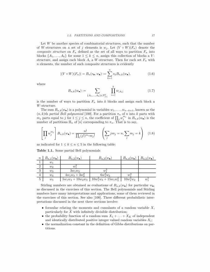
Table 1.1. Some partial Bell polynomials

n Bn,1(w•) Bn,2(w•) Bn,3(w•) Bn,4(w•) Bn,5(w•)1 w1

2 w2 w21

3 w3 3w1w2 w31

4 w4 4w1w3 + 3w22 6w2

1w2 w41

5 w5 5w1w4 + 10w2w3 10w21w3 + 15w1w

22 10w3

1w2 w51

Stirling numbers are obtained as evaluations of Bn,k(w•) for particular w•,as discussed in the exercises of this section. The Bell polynomials and Stirlingnumbers have many interpretations and applications, some of them reviewed inthe exercises of this section. See also [100]. Three different probabilistic inter-pretations discussed in the next three sections involve:

• formulae relating the moments and cumulants of a random variable X ,particularly for X with infinitely divisible distribution;

• the probability function of a random sum X1 + . . .+XK of independentand identically distributed positive integer valued random variables Xi;

• the normalization constant in the definition of Gibbs distributions on par-titions.

18 Jim Pitman

The second and third of these interpretations turn out to be closely related, andwill be of fundamental importance throughout this course. The first interpre-tation can be related to the second in special cases. But this interpretation israther different in nature, and not so closely connected to the main theme ofthe course.

Useful alternative expressions for Bn,k(w•) and Bn(v•, w•) can be given asfollows. For each partition of [n] into k disjoint non-empty blocks there arek! different ordered partitions of [n] into k such blocks. Corresponding to eachcomposition (n1, . . . , nk) of n with k parts, there are

(n

n1, . . . , nk

)

= n!

k∏

i=1

1

ni!

different ordered partitions (A1, . . . , Ak) of [n] with |Ai| = ni. So the definition(1.7) of Bn,k(w•) as a sum of products over partitions of [n] with k blocks implies

Bn,k(w•) =n!

k!

∑

(n1,...,nk)

k∏

i=1

wni

ni!(1.9)

where the sum is over all compositions of n into k parts. In view of this formula,it is natural to introduce the exponential generating functions associated withthe weight sequences v• and w•, say

v(θ) :=

∞∑

k=1

vkθk

k!and w(ξ) :=

∞∑

j=1

wjξj

j!

where the power series can either be assumed convergent in some neighborhoodof 0, or regarded formally. Then (1.9) reads

Bn,k(w•) =

[ξn

n!

]w(ξ)k

k!(1.10)

and (1.6) yields the formula

Bn(v•, w•) =

[ξn

n!

]

v(w(ξ)) (1.11)

known as the compositional or Faa di Bruno formula [407],[100, 3.4]. Thus thecombinatorial operation of composition of species of combinatorial structurescorresponds to the analytic operation of composition of exponential generatingfunctions. Note that (1.10) is the particular case of the compositional formula(1.11) when v• = 1(• = k), meaning vj = 1 if j = k and 0 else, for some1 ≤ k ≤ n. Another important case of (1.11) is the exponential formula [407]

Bn(x•, w•) =

[ξn

n!

]

exw(ξ) (1.12)

where x• is the sequence whose kth term is xk. For positive integer x, thisexponential formula gives the number of ways to partition the set [n] into anunspecified number of blocks, and assign each block of size j one of wj possiblestructures and one of x possible colors.

1.2. PARTITIONS AND COMPOSITIONS 19

Exercises

1.2.1. (Number of Compositions) [406, p. 14] The number of compositionsof n with k parts is

(n−1k−1

), and the number of compositions of n is 2n−1.

1.2.2. (Stirling numbers of the second kind) Let

Sn,k := Bn,k(1•) = #partitions of [n] into k blocks, (1.13)

where the substitution w• = 1• means wn = 1n ≡ 1. The numbers Sn,k areknown as Stirling numbers of the second kind.

n Sn,1 Sn,2 Sn,3 Sn,4 Sn,5

1 12 1 13 1 3 14 1 7 6 15 1 15 25 10 1

Show combinatorially that the Sn,k are the connection coefficients determinedby the identity of polynomials in x

xn =

n∑

k=1

Sn,k (x)k↓. (1.14)

1.2.3. (Stirling numbers of the first kind) Let

cn,k := Bn,k((• − 1)!) = #permutations of [n] with k cycles (1.15)

where the substitution w• = (• − 1)! means wn = (n− 1)!. Since (n− 1)! is thenumber of cyclic permutations of [n], the second equality in (1.15) corresponds tothe representation of a permutation of [n] as the product of cyclic permutationsacting on the blocks of some partition of [n]. The cn,k are known as unsignedStirling numbers of the first kind.

n cn,1 cn,2 cn,3 cn,4 cn,5

1 12 1 13 2 3 14 6 11 6 15 24 50 35 10 1

Show combinatorially that

(x)n↑ =

n∑

k=1

cn,k xk and (x)n↓ =

n∑

k=1

sn,kxk (1.16)

where the sn,k = (−1)n−kcn,k = Bn,k((−1)•−1(•− 1)!) are the Stirling numbersof the first kind. Check that the matrix of Stirling numbers of the first kind isthe inverse of the matrix of Stirling numbers of the second kind.

20 Jim Pitman

1.2.4. (Matrix representation of composition) Jabotinsky [100]. Regardthe numbers Bn,k(w•) for fixed w• as an infinite matrix indexed by n, k ≥ 1. Forsequences v• and w• with exponential generating functions v(ξ) and w(ξ), let(v w)• denote the sequence whose exponential generating function is v(w(ξ)).Then the matrix associated with the sequence (v w)• is the product of thematrices associated with w• and v• respectively. In particular, for w• with w1 6=0, and w−1

• the sequence whose exponential generating function w−1 is thecompositional inverse of w, so w−1(w(ξ)) = w(w−1(ξ)) = ξ, the matrix B(w−1

• )is the matrix inverse of B(w•).

1.2.5. (Polynomials of binomial type). Given some fixed weight sequencew•, define a sequence of polynomials Bn(x) by B0(x) := 1 and for n ≥ 1Bn(x) := Bn(x•, w•) as in (1.12). The sequence of polynomials Bn(x) is ofbinomial type, meaning that

n∑

j=0

(n

j

)

Bj(x)Bn−j(y) = Bn(x+ y). (1.17)

Conversely, it is known [391, 390] that if Bn(x) is a sequence of polynomials ofbinomial type such that Bn(x) is of degree n, then Bn(x) = Bn(x•, w•) as in(1.12) for some weight sequence w•. Note that then wj = [x]Bj(x).

1.2.6. (Change of basis) Each sequence of polynomials of binomial typeBn(x) with Bn of degree n defines a basis for the space of polynomials in x. Thematrix of connection coefficients involved in changing from one basis to anothercan be described in a number of different ways [391]. For instance, given twosequences of polynomials of binomial type, say Bn(x•, u•) and Bn(x•, v•), forsome weight sequences u• and v•, with v1 6= 0,

Bn(x•, u•) =

n∑

j=0

Bn,j(w•)Bj(x•, v•) (1.18)

where

w(ξ) := v−1(u(ξ)) is the unique solution of u(ξ) = v(w(ξ)).

for u and v the exponential generating functions associated with u• and v•.

1.2.7. (Generalized Stirling numbers) Toscano [415], Riordan [385, p. 46],Charalambides and Singh [89], Hsu and Shiue [203]. For arbitrary distinct reals

α and β, show that the connection coefficients Sα,βn,k defined by

(x)n↓α =n∑

k=0

Sα,βn,k (x)k↓β (1.19)

are

Sα,βn,k = Bn,k((β − α)•−1↓α) =

n!

k)k (1.20)

1.3. MOMENTS AND CUMULANTS 21

where

wα,β(ξ) :=∞∑

j=1

(β − α)j−1↓αξj

j!=

β−1((1 + αξ)β/α − 1) if α 6= 0, β 6= 0β−1(eβξ − 1) if α = 0α−1 log(1 + αξ) if β = 0.

(1.21)

n Sα,βn,1 Sα,β

n,2 Sα,βn,3 Sα,β

n,4

1 12 (β − α) 13 (β − α)(β − 2α) 3(β − α) 14 (β − α)(β − 2α)(β − 3α) 4(β − α)(β − 2α) + 3(β − α)2 6(β − α) 1

Alternatively

Sα,βn,k =

n∑

j=k

sn,jSj,kαn−jβj−k (1.22)

where sn,j := S1,0n,j is a Stirling number of the first kind and Sj,k := S0,1

j,k is aStirling number of the second kind.

1.3. Moments and cumulants

Let (Xt, t ≥ 0) be a real-valued Levy process, that is a process with stationaryindependent increments, started at X0 = 0, with sample paths which are cadlag(right continuous with left limits) [40]. According to the exponential formula ofprobability theory, i.e. the Levy-Khintchine formula, if we assume that Xt hasa convergent moment generating function in some neighborhood of 0 then

E[eθXt ] = exp (tΨ(θ)) (1.23)

for a characteristic exponent Ψ which can be represented as

Ψ(θ) =

∞∑

n=1

κnθn

n!(1.24)

where κ1 = E(X1), κ2 is the variance of X1, and

κn =

∫

R

xnΛ(dx) (n = 3, 4, . . .). (1.25)

where Λ is the Levy measure ofX1. Compare (1.23) with the exponential formulaof combinatorics (1.12) to see that the coefficient of θn/n! in (1.23) is

E(Xnt ) = Bn(t•, κ•). (1.26)

Thus the moments of Xt define a sequence of polynomials in t which is thesequence of polynomials of binomial type associated with the sequence κ• ofcumulants of X1. Two special cases are worthy of note.

22 Jim Pitman

Gaussian case If X1 is standard Gaussian, the sequence of cumulants of X1

is κ• = 1(• = 2). It follows from (1.26) and the combinatorial meaning of Bn,k

that the nth moment µn of X1 is the number of matchings of [n], meaning thenumber of partitions of [n] into n/2 pairs. Thus

E(Xnt )/tn/2 =

0 if n is odd1× 3× · · · (n− 1) if n is even.

(1.27)

Exercise 1.3.4 and Exercise 1.3.5 offer some generalizations.

Poisson case If X1 = N1 is Poisson with mean 1, the sequence of cumulantsis κ• = 1•. The positive integer moments of Nt are therefore given by

E(Nnt ) =

∞∑

m=0

e−ttmmn

m!=

n∑

k=1

Bn,k(1•)tk (n = 1, 2, . . .) (1.28)

where the Bn,k(1•) are the Stirling numbers of the second kind. These polyno-mials in t are known as exponential polynomials. In particular, the nth momentof the Poisson(1) distribution of N1 is the nth Bell number

Bn(1•, 1•) :=n∑

k=1

Bn,k(1•) =

[ξn

n!

]

exp(eξ − 1)

which is the number of partitions of [n]. The first six Bell numbers are

1, 2, 5, 15, 52, 203.

Now (1.28) for t = 1 gives the famous Dobinski formula [111]

Bn(1•, 1•) = e−1∞∑

m=1

mn

m!. (1.29)

As noted by Comtet [100], for each n the infinite sum in (1.29) can be evaluatedas the least integer greater than the sum of the first 2n terms.

Exercises

1.3.1. (Moments and Cumulants) [290, 100] Let X1 be any random variablewith a moment generating function which is convergent in some neighborhood of0. Let µn := E(Xn

1 ) and let the cumulants κn of X1 be defined by the expansion(1.24) of Ψ(θ) := log E[eθX1 ]. Show that the moment and cumulant sequencesµ• and κ• determine each other by the formulae

µn =

n∑

k=1

Bn,k(κ•) and κn =

n∑

k=1

(−1)k−1(k − 1)!Bn,k(µ•) (1.30)

for n = 1, 2, . . .. These formulae allow the first n cumulants of X to be definedfor anyX with E[|X |n] <∞, and many of the following exercises can be adaptedto this case.

1.3. MOMENTS AND CUMULANTS 23

1.3.2. (Thiele’s recursion) [186, p. 144, (4.2)], [316, p.74, Th. 2], [107, Th.2.3.6]. Two sequences µ• and κ• are related by (1.30) if and only if

µn =

n−1∑

i=0

(n− 1

i

)

µiκn−i (n = 1, 2, . . .) (1.31)

where µ0 = 0.

1.3.3. (Moment polynomials) [77], [187], [319, p. 80], [146] [147, Prop. 2.1.4].For t = 1, 2, . . . let St =

∑ti=1 Xi where the Xi are independent copies of X

with moment sequence µ• and cumulant sequence κ•. Then

E[Snt ] =

n∑

k=1

Bn,k(κ•)tk =

n∑

k=1

Bn,k(µ•)(t)k↓. (1.32)

For n = 0, 1, . . ., and x real, let

µn(x, t) := E[(x + St)n] =

n∑

k=0

(n

k

)

xkE[Sn−k

t ] (t = 0, 1, 2, . . .) (1.33)

where S0 := 0, and let

Hn(x, t) := µn(x,−t) (1.34)

where the right side is defined for each x by polynomial continuation of µn(x, t)in (1.33). Then

(Hn(St, t), t = 0, 1, 2, . . .) is an (Ft)-martingale (1.35)

where Ft is the σ-field generated by (Su, u = 0, 1, . . . , t).

1.3.4. (Matchings and Stirling numbers). Check that for X1 standardGaussian (1.32) for even n = 2q gives

E(S2qt ) = tqµ2q =

q∑

k=1

B2q,k(µ•)(t)k↓. (1.36)

Compare with the definition (1.16) of Stirling numbers of the second kind tosee that

B2q,k(µ•) = µ2qBq,k(1•). (1.37)

Give a combinatorial proof of (1.37) and deduce more generally that

B2q,k(µ•x•/2) = µ2qB2q,k(x•) (1.38)

for an arbitrary sequence x•, where the nth term of µ•x•/2 is µqxq if n = 2q iseven, and 0 else.

24 Jim Pitman

1.3.5. (Feynman diagrams) [214, Theorem 1.28] [297, Lemma 4.5]. Check thefollowing generalization of (1.27): if X1, . . . , Xn are centered jointly Gaussianvariables, then

E(X1 · · ·Xn) =∑∏

k

E(XikXjk

) (1.39)

where the sum is over all partitions of [n] into n/2 pairs ik, jk, 1 ≤ k ≤ n/2.See [297] for applications to local times of Markov processes.

1.3.6. (Poisson moments)[353] Deduce (1.28) from (1.16) and the more ele-mentary formula E[(Nt)n↓] = tn.

Notes and comments

Moment calculations for commutative and non-commutative Gaussian randomvariables in terms of partitions, matchings etc. are described in [196]. There, forinstance, is a discussion of the fact that the Catalan numbers are the momentsof the semicircle law, which appears in Wigner’s limit theorem for the empiricaldistribution of the eigenvalues of a random Hermitian matrix. Combinatorialrepresentations for the moments of superprocesses, in terms of expansions overforests, were given by Dynkin [129], where a connection is made with similar cal-culations arising in quantum field theory. This is further explained with picturesin Etheridge [136]. These ideas are further applied in [139, 140, 388].

1.4. Random sums

Recall that if X , X1, X2, . . . are independent and identically distributed non-negative integer valued random variables with probability generating function

GX (z) := E[zX ] =

∞∑

n=0

P(X = n)zn,

andK is a non-negative integer valued random variable independent ofX1, X2, . . .with probability generating function GK , and SK := X1 + · · · + XK , then, byconditioning on K, the probability generating function of SK is found to be thecomposition of GK and GX :

GSK(z) = GK(GX (z)). (1.40)

Comparison of this formula with the compositional formula (1.11) for Bn(v•, w•)in terms of the exponential generating functions v(z) =

∑∞n=0 vnz

n/n! andw(ξ) =

∑∞n=1 wnξ

n/n!, suggests the following construction. (It is convenienthere to allow v0 to be non-zero, which makes no difference in (1.11)). Let ξ > 0 besuch that v(w(ξ)) <∞. Let Pξ,v•,w•

be a probability distribution which makesXi independent and identically distributed with the power series distribution

Pξ,v•,w•(X = n) =

wnξn

n!w(ξ)for n = 1, 2, . . . , so GX(z) =

w(zξ)

w(ξ)(1.41)

1.5. GIBBS PARTITIONS 25

and K independent of the Xi with the power series distribution

Pξ,v•,w•(K = k) =

vkw(ξ)k

k!v(w(ξ))for k = 0, 1, 2, . . . so GK(y) =

v(yw(ξ))

v(w(ξ)). (1.42)

Let SK := X1 + · · ·+XK . Then from (1.40) and (1.11),

Pξ,v•,w•(SK = n) =

ξn

n!v(w(ξ))Bn(v•, w•) (1.43)

or

Bn(v•, w•) =n!v(w(ξ))

ξnPξ,v•,w•

(SK = n) (1.44)

This probabilistic representation of Bn(v•, w•) was given in increasing generalityby Holst [201], Kolchin [260], and Kerov [240]. Renyi’s formula for the Bellnumbers Bn(1•, 1•) in Exercise 1.4.1 is a variant of (1.44) for v• = w• = 1•.Holst [201] gave (1.44) for v• and w• with values in 0, 1, when Bn(v•, w•) isthe number of partitions of [n] into some number of blocks k with vk = 1 andeach block of size j with wj = 1. As observed by Renyi and Holst, for suitablev• and w• the probabilistic representation (1.44) allows large n asymptotics ofBn(v•, w•) to be derived from local limit approximations to the distribution ofsums of independent random variables. This method is closely related to classicalsaddle point approximations: see notes and comments at the end of Section 1.5.

Exercises

1.4.1. (Renyi’s formula for the Bell numbers)[382, p. 11]. Let (Nt, t ≥ 0)and (Mt, t ≥ 0) be two independent standard Poisson processes. Then for n =1, 2, . . . the number of partitions of [n] is

Bn(1•, 1•) = n! ee−1P(NMe

= n). (1.45)

1.4.2. (Asymptotic formula for the Bell numbers)[288, 1.9]. Deduce from(1.45) the asymptotic equivalence

Bn(1•, 1•) ∼ 1√nλ(n)n+1/2eλ(n)−n−1 as n→∞, (1.46)

where λ(n) log(λ(n)) = n.

1.5. Gibbs partitions

Suppose as in Section 1.2 that (V W )([n]) is the set of all composite V W -structures built over [n], for some species of combinatorial structures V and W .Let a composite structure be picked uniformly at random from (V W )([n]), and

26 Jim Pitman

let Πn denote the random partition of [n] generated by blocks of this randomcomposite structure. Recall that vj and wj denote the number of V - and W -structures respectively on a set of j elements. Then for each particular partitionA1, . . . , Ak of [n] it is clear that

P(Πn = A1, . . . , Ak) = p(|A1|, . . . , |Ak|; v•, w•) (1.47)

where for each composition (n1, . . . , nk) of n

p(n1, . . . , nk; v•, w•) :=vk

∏ki=1 wni

Bn(v•, w•)(1.48)

with the normalization constant Bn(v•, w•) :=∑n

k=1 vkBn,k(w•) as in (1.6)and (1.11), assumed strictly positive. More generally, given two non-negativesequences v• := (v1, v2, . . .) and w• := (w1, w2, . . .), call Πn a Gibbs[n](v•, w•)partition if the distribution of Πn on P[n] is given by (1.47)-(1.48). Note thatdue to the normalization in (1.48), there is the following redundancy in theparameterization of Gibbs[n](v•, w•) partitions: for arbitrary positive constantsa, b and c,

Gibbs[n](ab•v•, c

•w•) = Gibbs[n](v•, bw•). (1.49)

That is to say, the Gibbs[n](v•, w•) distribution is unaffected by multiplyingv• by a constant factor a, or multiplying w• by a geometric factor c•, whilemultiplying v• by the geometric factor b• is equivalent to multiplication of w•by the constant factor b.

The block sizes in exchangeable order The following theorem provides afundamental representation of Gibbs partitions.

Theorem 1.2. (Kolchin’s representation of Gibbs partitions) [260], [240]Let (N ex

n,1, . . . , Nexn,|Π|n) be the random composition of n defined by putting the

block sizes of a Gibbs[n](v•, w•) partition Πn in an exchangeable random order,meaning that given k blocks, the order of the blocks is randomized by a uniformrandom permutation of [k]. Then

(N exn,1, . . . , N

exn,|Π|n)

d= (X1, . . . , XK) under Pξ,v•,w•

given X1 + · · ·+XK = n(1.50)

where Pξ,v•,w•governs independent and identically distributed random variables

X1, X2, . . . with E(zXi) = w(zξ)/w(ξ) and K is independent of these variableswith E(yK) = v(yw(ξ))/v(w(ξ)) as in (1.41) and (1.42).

Proof. It is easily seen that the manipulation of sums leading to (1.9) can beinterpreted probabilistically as follows:

P((N exn,1, . . . , N

exn,|Π|n) = (n1, . . . , nk)) =

n! vk

k!Bn(v•, w•)

k∏

i=1

wni

ni!(1.51)

for all compositions (n1, . . . , nk) of n. Compare with formula (1.43) and theconclusion is evident.

1.5. GIBBS PARTITIONS 27

Note that for fixed v• and w•, the Pξ,v•,w•distribution of the random integer

composition (X1, . . . , XK) depends on the parameter ξ, but the Pξ,v•,w•condi-

tional distribution of (X1, . . . , XK) given SK = n does not. In statistical terms,with v• and w• regarded as fixed and known, the sum SK is a sufficient statisticfor ξ. Note also that for any fixed n, the distribution of Πn depends only onthe weights vj and wj for j ≤ n, so the condition v(w(ξ)) < ∞ can always bearranged by setting vj = wj = 0 for j > n.

The partition of n Recall that the random partition of n induced by arandom partition Πn of [n] is encoded by the random vector (|Πn|j , 1 ≤ j ≤ n)where |Πn|j is the number of blocks of Πn of size j. Using (1.8), the distributionof the partition of n induced by a Gibbs[n](v•, w•) partition Πn is given by

P(|Πn|j = mj , 1 ≤ j ≤ n) =n! vk

Bn(v•, w•)

n∏

j=1

(wj

j!

)mj 1

mj !(1.52)

where∑n

j=1 mj = k and∑n

j=1 jmj = n. In particular, for a Gibbs[n](1•, w•)

partition

(|Πn|j , 1 ≤ j ≤ n)d=

Mj , 1 ≤ j ≤ n

∣∣∣∣∣∣

n∑

j=1

jMj = n

(1.53)

where the Mj are independent Poisson variables with parameters (wjξj/j!) for

arbitrary ξ > 0. This can also be read from (1.50). For v• = 1• the random vari-able K has Poisson (w(ξ)) distribution. Hence, by the classical Poissonization ofthe multinomial distribution, the number Mj of i such that i ≤ K and Xi = jhas a Poisson (wjξ

j/j!) distribution, and SK =∑

j jMj is compound Poisson.See also Exercise 1.5.1 . Arratia, Barbour and Tavare [27] make the identity indistribution (1.53) the starting point for a detailed analysis of the asymptoticbehaviour of the counts (|Πn|j , 1 ≤ j ≤ n) of a Gibbs[n](1

•, w•) partition asn→∞ for w• in the logarithmic class, meaning that jwj/j!→ θ as j →∞ forsome θ > 0. One of their main results is presented later in Chapter 2.

Physical interpretation Suppose that n particles labeled by elements of theset [n] are partitioned into clusters in such a way that each particle belongs to aunique cluster. Formally, the collection of clusters is represented by a partitionof [n]. Suppose further that each cluster of size j can be in any one of wj

different internal states for some sequence of non-negative integers w• = (wj).Let the configuration of the system of n particles be the partition of the set of nparticles into clusters, together with the assignment of an internal state to eachcluster. For each partition π of [n] with k blocks of sizes n1, . . . , nk, there are∏k

i=1 wnidifferent configurations with that partition π. So Bn,k(w•) gives the

number of configurations with k clusters. For v• = 1(• = k) the sequence withkth component 1 and all other components 0, the Gibbs(v•, w•) partition of [n]corresponds to assuming that all configurations with k clusters are equally likely.

28 Jim Pitman

This distribution on the set Pk[n] of partitions of [n] with k blocks, is known in

the physics literature as a microcanonical Gibbs state. It may also be called herethe Gibbs(w•) distribution on Pk

[n]. A general weight sequence v• randomizesk, to allow any probabilistic mixture over k of these microcanonical states. Forfixed w• and n, the set of all Gibbs(v•, w•) distributions on partitions of [n], asv• varies, is an (n − 1)-dimensional simplex whose set of extreme points is thecollection of n different microcanonical states. Whittle [432, 433, 434] showedhow the Gibbs distribution (1.52) on partitions of n arises as the reversibleequilibrium distribution in a Markov process with state space Pn, where parts ofvarious sizes can split or merge at appropriate rates. In this setting, the Poissonvariables Mj represent equilibrium counts in a corresponding unconstrainedsystem where the total size is also subject to variation. See also [123] for furtherstudies of equilibrium models for processes of coagulation and fragmentation.

Example 1.3. Uniform random set partitions. Let Πn be a uniformlydistributed random partition of [n]. Then Πn is a random (V V )-structureon [n] for V the species of non-empty sets. Thus Πn has the Gibbs(1•, 1•)distribution on P[n]. Note that P(|Πn| = k) = Bn,k(1•)/Bn(1•, 1•) but there isno simple formula, either for the Stirling numbers of the second kind Bn,k(1•),or for the Bell numbers Bn(1•, 1•). Exercise 1.5.5 gives a normal approximationfor |Πn|. The independent and identically distributed variables Xi in Kolchin’srepresentation are Poisson variables conditioned not to be 0. See [159, 174, 424]and papers cited there for further probabilistic analysis of Πn for large n.

Example 1.4. Random permutations. Let W (F ) be the set of all permu-tations of F with a single cycle. Then wn = (n− 1)!, so

w(ξ) =

∞∑

n=1

(n− 1)!ξn

n!= − log(1− ξ)

and

eθw(ξ) = e−θ log(1−ξ) = (1− ξ)−θ =

∞∑

n=0

(θ)n↑1ξn

n!.

So

Bn(1•, θ(• − 1)!) = (θ)n↑1. (1.54)

In particular, for θ = 1, Bn(1•, (•−1)!) = (1)n↑1 = n! is just the number of per-mutations of [n]. Since each permutation corresponds bijectively to a partitionof [n] and an assignment of a cycle to each block of the partition, the randompartition Πn of [n] generated by the cycles of a uniform random permutation of[n] is a Gibbs[n](1

•, (•− 1)!) partition. While there is no simple formula for theunsigned Stirling numbers Bn,k((• − 1)!) which determine the distribution of|Πn|, asymptotic normality of this distribution is easily shown ( Exercise 1.5.4). Similarly, for θ = 1, 2, . . . the number in (1.54) is the number of different waysto pick a permutation of [n] and assign each cycle of the permutation one ofθ possible colors. If each of these ways is assumed equally likely, the resulting

1.5. GIBBS PARTITIONS 29

random partition of [n] is a Gibbs[n](1•, θ(• − 1)!) partition. For any θ > 0, the

Xi in Kolchin’s representation have logarithmic series distribution

pj =1

− log(1− b)bj

j(j = 1, 2, . . .)

where 0 < b < 1 is a positive parameter. This example is developed further inChapter 3.

Example 1.5. Cutting a rooted random segment. Suppose that the inter-nal state of a cluster C of size j is one of wj = j! linear orderings of the set C.Identify each cluster as a directed graph in which there is a directed edge froma to b if and only if a is the immediate predecessor of b in the linear ordering.Call such a graph a rooted segment. Then Bn,k(•!) is the number of directed

4 2 3 651

4 2 3 651

4 2 3 651

4 2 3 651

4 2 3 651

4 2 3 651

Figure 1.1: Cutting a rooted random segment

graphs labeled by [n] with k such segments as its connected components. In theprevious two examples, with wj = 1j and wj = (j − 1)!, the Bn,k(w•) wereStirling numbers for which there is no simple formula. Since j! = (β − α)j−1↓α

for α = −1 and β = 1, formula (1.20) shows that the Bell matrix Bn,k(•!) is thearray of generalized Stirling numbers

Bn,k(•!) = S−1,1n,k =

(n− 1

k − 1

)n!

k!(1.55)

known as Lah numbers [100, p. 135], though these numbers were already con-sidered by Toscano [415]. The Gibbs model in this instance is a variation ofFlory’s model for a linear polymerization process. It is easily shown in thiscase that a sequence of random partitions (Πn,k, 1 ≤ k ≤ n) such that Πn,k

has the microcanonical Gibbs distribution on clusters with k components maybe obtained as follows. Let G1 be a uniformly distributed random rooted seg-ment labeled by [n]. Let Gk be derived from G1 by deletion of a set of k − 1edges picked uniformly at random from the set of n − 1 edges of G1, and let

30 Jim Pitman

Πn,k be the partition induced by the components of Gk . If the n − 1 edges ofG1 are deleted sequentially, one by one, cf. Figure 1.1, the random sequence(Πn,1,Πn,2, . . . ,Πn,n) is a fragmenting sequence, meaning that Πn,j is coarserthan Πn,k for j < k, such that Πn,k has the microcanonical Gibbs distributionon Pk

[n] derived from the weight sequence wj = j!. The time-reversed sequence

(Πn,n,Πn,n−1, . . . ,Πn,1) is then a discrete time Markov chain governed by therules of Kingman’s coalescent [30, 253]: conditionally given Πk with k compo-nents, Πk−1 is equally likely to be any one of the

(k2

)different partitions of [n]

obtained by merging two of the components of Πk. Equivalently, the sequence(Πn,1,Πn,2, . . . ,Πn,n) has uniform distribution over the set Rn of all fragment-ing sequences of partitions of [n] such that the kth term of the sequence has kcomponents. The consequent enumeration #Rn = n!(n−1)!/2n−1 was found byErdos et al. [135]. That Πn,k determined by this model has the microcanonicalGibbs(•!) distribution on Pk

[n] was shown by Bayewitz et. al. [30] and Kingman

[253]. See also Chapter 5regarding Kingman’s coalescent with continuous timeparameter.

Example 1.6. Cutting a rooted random tree. Suppose the internal stateof a cluster C of size j is one of the wj = jj−1 rooted trees labeled by C. ThenBn,k(••−1) is the number of forests of k rooted trees labeled [n]. This time againthere is a simple construction of the microcanonical Gibbs states by sequentialdeletion of random edges, hence a simple formula for Bn,k.

6

5 2

3

4

1 6

5 2

3

4

1 6

5 2

3

4

1 6

5 2

3

4

1 6

5 2

3

4

1 6

5 2

3

4

1

Figure 1.2: Cutting a rooted random tree with 5 edges

By a reprise of the previous argument [356],

Bn,k(••−1) =

(n

k

)

knn−k−1 (1.56)

which is an equivalent of Cayley’s formula knn−k−1 for the number of rootedtrees labeled by [n] whose set of roots is [k]. The Gibbs model in this instancecorresponds to assuming that all forests of k rooted trees labeled by [n] areequally likely. This model turns up naturally in the theory of random graphsand has been studied and applied in several other contexts. The coalescentobtained by reversing the process of deletion of edges is the additive coalescentstudied in [356]. The structure of large random trees is one of the main themesof this course, to be taken up in Chapter 6. This leads in Chapter 7 to thenotion of continuum trees embedded in Brownian paths, then in Chapter 10 toa representation in terms of continuum trees of the large n asymptotics of theadditive coalescent.

1.5. GIBBS PARTITIONS 31

Gibbs fragmentations Let p(λ | k) denote the probability assigned to a par-tition λ of [n] by the microcanonical Gibbs distribution on Pk

[n] with weights w•,

that is p(λ | k) = 0 unless λ is a partition of of [n] into k blocks of sizes sayni(λ), 1 ≤ i ≤ k, in which case

p(λ | k) =1

Bn,k(w•)

k∏

i=1

wni(λ) (1.57)

The simple evaluation of Bn,k(w•) in the two previous examples, for wn = (n−1)! and wn = nn−1 respectively, was related to a simple sequential constructionof a Gibbs(w•) fragmentation process, that is a sequence of random partitions

(Πn,1,Πn,2, . . . ,Πn,n)

such that Πn,k has the Gibbs(w•) distribution on Pk[n], and for each 1 ≤ k ≤

n − 1 the partition Πn,k is a refinement of Πn,k−1 obtained by splitting someblock Πn,k−1 in two. This leads to the question of which weight sequences(w1, . . . , wn−1) are such that there exists a Gibbs(w•) fragmentation process. Isthere exists such a process, then one can also be constructed as a Markov chainwith some transition matrix P (π, ν) indexed by P[n] such that P (π, ν) > 0 onlyif ν is a refinement of π, and

∑

ν∈P[n]

p(π|k − 1)P (π, ν) = p(ν | k) (1 ≤ k ≤ n− 1). (1.58)

Such a transition matrix P (π, ν) corresponds to a splitting rule, which for each1 ≤ k ≤ n − 1, and each partition π of [n] into k − 1 components, describesthe probability that π splits into a partition ν of [n] into k components. Giventhat Πk−1 = A′

1, . . . , A′k−1 say, the only possible values of Πk are partitions

A1, . . . , Ak such that two of the Aj , say A1 and A2, form a partition of oneof the A′

i, and the remaining Aj are identical to the remaining A′i. The initial

splitting rule starting with π1 = 1, . . . , n is described by the Gibbs formulap(· | 2) determined by the weight sequence (w1, . . . , wn−1). The simplest way tocontinue is to use the followingRecursive Gibbs Rule: whenever a component is split, given that the componentcurrently has size m, it is split according to the Gibbs formula p(n1, n2 | 2) forn1 and n2 with n1 + n2 = n.

To complete the description of a splitting rule, it is also necessary to specifyfor each partition πk−1 = A′

1, . . . , A′k−1 the probability that the next com-

ponent to be split is A′i, for each 1 ≤ i ≤ k − 1. Here the simplest possible

assumption seems to be the following:Linear Selection Rule: Given πk−1 = A′

1, . . . , A′k−1, split A′

i with probabilityproportional to #Ai − 1.

While this selection rule is somewhat arbitrary, it is natural to investigate itsimplications for the following reasons. Firstly, components of size 1 cannot besplit, so the probability of picking a component to split must depend on size. This

32 Jim Pitman

probability must be 0 for a component of size 1, and 1 for a component of sizen− k+ 2. The simplest way to achieve this is by linear interpolation. Secondly,both the segment splitting model and the tree splitting model described inExamples 1.5 and 1.6 follow this rule. In each of these examples a componentof size m is derived from a graph component with m − 1 edges, so the linearselection rule corresponds to picking an edge uniformly at random from theset of all edges in the random graph whose components define Πk−1. Giventwo natural combinatorial examples with the same selection rule, it is naturalask what other models there might be following the same rule. At the level ofrandom partitions of [n], this question is answered by the following proposition.It also seems reasonable to expect that the conclusions of the proposition willremain valid under weaker assumptions on the selection rule.

Proposition 1.7. Fix n ≥ 4, let (wj , 1 ≤ j ≤ n − 1) be a sequence of pos-itive weights with with w1 = 1, and let let (Πk, 1 ≤ k ≤ n) be a P[n]-valuedfragmentation process defined by the recursive Gibbs splitting rule derived fromthese weights, with the linear selection rule. Then the following statements areequivalent:

(i) For each 1 ≤ k ≤ n the random partition Πk has the Gibbs distributionon Pk

[n] derived from (wj , 1 ≤ j ≤ n− 1);

(ii) The weight sequence is of the form

wj =

j∏

m=2

(mc+ jb) (1.59)

for every 1 ≤ j ≤ n− 1 for some constants c and b.

(iii) For each 2 ≤ k ≤ n, given that Πk has k components of sizes n1, · · · , nk,the partition Πk−1 is derived from Πk by merging the ith and jth of these com-ponents with probability proportional to 2c+ b(ni +nj) for some constants c andb.

The constants c and b appearing in (ii) and (iii) are only unique up to con-stant factors. To be more precise, if either of conditions (ii) or (iii) holds forsome (b, c), then so does the other condition with the same (b, c). Hendriks etal. [195] showed that the construction (iii) of a P[n]-valued coalescent process(Πn,Πn−1, . . . ,Π1) corresponds to the discrete skeleton of the continuous timeMarcus-Lushnikov model with state space Pn and merger rate 2c + b(x + y)between every pair of components of sizes (x, y), and that the distribution ofΠk is then determined as in (i) and (ii). Note the implication of Proposition 1.7that if (Πn,Πn−1, . . . ,Π1) is so constructed as a coalescent process, then thereversed process (Π1,Π2, . . . ,Πn) is a Gibbs fragmentation process governed bythe recursive Gibbs splitting rule with weights (wj) as in (ii) and linear selectionprobabilities.

Lying behind Proposition 1.7 is the following evaluation of the associatedBell polynomial:

1.5. GIBBS PARTITIONS 33

Lemma 1.8. For wj =∏j

m=2(mc+ jb), j = 2, 3, . . .

Bn,k(1, w2, w3, . . .) =

(n− 1

k − 1

) n∏

m=k+1

(mc+ nb) (1 ≤ k ≤ n). (1.60)

This evaluation can be read from [195, (19)-(21)]. The full proof of Proposi-tion 1.7 will be given elsewhere.

Example 1.9. Random mappings. Let Mn be a uniformly distributed ran-dom mapping from [n] to [n], meaning that all nn such maps are equally likely.Let Πn the partition of [n] induced by the tree components of the usual func-tional digraph of Mn. Then Πn is the random partition of [n] associated arandom (V W )-structure on [n] for V the species of permutations and W thespecies of rooted labeled trees. So Πn has the Gibbs(•!, ••−1) distribution onP[n]. Let Πn denote the partition of [n] induced by the connected components

of the usual functional digraph of Mn, so each block of Πn is the union of treecomponents in Πn attached to some cycle of Mn. Then Πn is the random parti-tion of [n] derived from a random (V W )-structure on [n] for V the species ofnon-empty sets and W the species of mappings whose digraphs are connected.So Πn has a Gibbs(1•, w•) distribution on P[n] where wj is the number of map-pings on [j] whose digraphs are connected. Classify by the number c of cyclicpoints of the mapping on [j], and use (1.56), to see that

wj =

j∑

c=1

(c− 1)!

(j

c

)

cjj−c−1 = P(Nj < j)(j − 1)!ej ∼ 12 (j − 1)!ej as j →∞

(1.61)where Nj is a Poisson(j) variable. This example is further developed in Chapter9.

Exercises

1.5.1. (Compound Poisson) Stam [404]. Let ∆1, ∆2, . . . denote the successivejumps of a non-negative integer valued compound Poisson process (X(t), t ≥ 0)with jump intensities λj , j = 1, 2, . . ., with λ :=

∑

j λj ∈ (0,∞), and let N(t)

be the number of jumps of X in [0, t], so that Xt =∑Nt

i=1 ∆i. The ∆i areindependent and identically distributed with distribution P (∆i = j) = λj/λ,independent of N(t), hence

P(X(t) = n |N(t) = k) = λk∗n /λk

where (λk∗n ) is the k-fold convolution of the sequence (λn) with itself, with the

convention λ0∗n = 1(n = 0). So for all t ≥ 0 and n = 0, 1, 2, . . .

P[X(t) = n] = e−λtn∑

k=0

λk∗n

tk

k!=e−λt

n!Bn(t•, w•) for wj := j!λj . (1.62)

34 Jim Pitman

Moreover for each t > 0 and each n = 1, 2, . . .,

(∆1, . . . ,∆N(t)) given X(t) = n (1.63)

has the exchangeable Gibbs distribution on compositions of n defined by (1.51)for vk ≡ 1 and wj := tj!λj . Let Nj(t) be the number of i ≤ N(t) such that∆i = j. Then the Nj(t) are independent Poisson variables with means λjt.The random partition of n derived from the random composition (1.63) of n isidentical to

(Nj(t), 1 ≤ j ≤ n) given

∞∑

j=1

jNj(t) = n, (1.64)

and the distribution of (Nj(t), 1 ≤ j ≤ n) remains the same with conditioningon∑n

j=1 jNj(t) = n instead of∑∞

j=1 jNj(t) = n.

1.5.2. (Distribution of the number of blocks) For a Gibbs(1•, w•) partitionof [n],

P(|Πn| = k) =Bn,k(w•)

Bn(w•)=n!

k!

(w(ξ))k

ξnBn(w•)Pξ,w•

(Sk = n) (1.65)

for 1 ≤ k ≤ n, where Pξ,w•governs Sk as the sum of k independent variables

Xi with the power series distribution (1.41), assuming that ξ > 0 is such thatw(ξ) < ∞, and the complete Bell polynomial Bn(1•, w•) :=

∑nk=1 Bn,k(w•) is

determined via the exponential formula (1.12). Deduce from (1.65) the formula[99]

E(|Πn|) =1

Bn(1•, w•)

[ξn

n!

]

w(ξ)ew(ξ). (1.66)

Kolchin [260, §1.6] and other authors [317], [99] have exploited the representation(1.65) to deduce asymptotic normality of |Πn| for large n, under appropriateassumptions on w•, from the asymptotic normality of the Pξ,w•

asymptoticdistribution of Sk for large k and well chosen ξ, which is typically determinedby a local limit theorem. See also [27] for similar results obtained by othertechniques.

1.5.3. (Normal approximation for combinatorial sequences: Harper’smethod)

(i) (Levy) Let (a0, a1, . . . an) be a sequence of nonnegative real numbers, withgenerating polynomial A(z) :=

∑nk=0 akz

k, z ∈ C, such that A(1) > 0.Show that A has only real zeros if and only if there exist independentBernoulli trials X1, X2, . . . , Xn with P (Xi = 1) = pi ∈ (0, 1], 1 ≤ i ≤ n,such that P (X1 +X2 + · · ·+Xn = k) = ak/A(1), ∀ 0 ≤ k ≤ n. Then theroots αi of A are related to the pi by αi = −(1− pi)/pi.

(ii) (Harper, [190]) Let an,knk=0 be a sequence of nonnegative real numbers.Suppose that Hn(z) :=

∑nk=0 an,kz

k, z ∈ C with Hn(1) > 0 has only realroots, say αn,i = −(1− pn,i)/pn,i. Suppose Kn is a random variable withdistribution

Pn(k) := P (Kn = k) = an,k/Hn(1) (0 ≤ k ≤ n).

1.5. GIBBS PARTITIONS 35

ThenKn − µn

σn

d→ N(0, 1) if and only if σn →∞,

where µn := E (Kn) =∑n

i=1 pn,i, and σ2n := Var (Kn) =

∑ni=1 pn,i(1 −

pn,i). See [352] and papers cited there for numerous applications. Twobasic examples are provided by the next two exercises. Harper [190] alsoproved a local limit theorem for such a sequence provided the central limittheorem holds. Hence both kinds of Stirling numbers admit local normalapproximations.

1.5.4. (Number of cycles of a uniform random permutation) Let an,k =Bn,k ((• − 1)!) be the Stirling numbers of the first kind, note from (1.14) that

Hn(z) = z(z + 1)(z + 2) · · · (z + n− 1)

Deduce that if Kn is the number of cycles from a uniformly chosen permutationof [n] then the Central Limit Theorem holds, E (Kn)− logn = O(1), Var (Kn) ∼logn, and hence

Kn − logn√logn

d→ N(0, 1).

1.5.5. (Number of blocks of a uniform random partition) Let an,k =Bn,k (1•) be the Stirling numbers of the second kind. Let Kn be the number ofblocks of a uniformly chosen partition of [n].

(a) Show that Bn+1,k(1•) = Bn,k−1(1•) + k Bn,k(1•).(b) Using (a) deduce that

ezHn+1(z) = zd

dz(ezHn(z)) .

(c) Apply induction to show that for all n ≥ 1, Hn has only real zeros.(d) Use the recursion in (a) again to show

µn := E [Kn] =Bn+1

Bn− 1, and

σ2n := Var (Kn) =

Bn+2

Bn−(Bn+1

Bn

)2

− 1,

where Bn := Hn(1) = Bn(1•, 1•) is the nth Bell number.(e) Deduce the Central Limit Theorem.

1.5.6. (Problem: existence of Gibbs fragmentations) For given w•, de-scribe the set of n for which such a fragmentation process exists. In particular,for which w• does such a process exist for all n? Even the following particularcase for wj = (j − 1)! does not seem easy to resolve:

1.5.7. (Problem: cyclic fragmentations) Does there exist for each n a Pn-valued fragmentation process (Πn,k, 1 ≤ k ≤ n) such that Πn,k is distributedlike the partition generated by cycles of a uniform random permutation of [n]conditioned to have k cycles?

1.5.8. Show that for w• = 1•, for all sufficiently large n there does not exist aGibbs(w•) fragmentation process of [n]. [Hint: Πn,k has the same distributionas the partition generated by n independent random variables with uniformdistribution on [k], conditioned on the event that all k values appear].

1.5.9. (Problem) For exactly which n does there exist a Gibbs(1•) fragmen-tation process of [n]? What is the largest such n?

Notes and comments

See also Bender [31, 32] and Canfield [83] for more general analytic methodsto obtain central and local limit theorems for combinatorial sequences. Canfield[83] gives nice sufficient conditions for central and local limit theorems for thecoefficients of polynomials of binomial type. Similar results may also be derivedusing classical analytic techniques like the saddle point approximation [333] andHayman’s criterion [194].

36

1.5. GIBBS PARTITIONS 37

38 Jim Pitman

Chapter 2

Exchangeable random

partitions

This chapter is a review of basic ideas from Kingman’s theory of exchangeablerandom partitions [253], as further developed in [14, 347, 350]. This theoryturns out to be of interest in a number of contexts, for instance in the study ofpopulation genetics, Bayesian statistics, and models for processes of coagulationand fragmentation. The chapter is arranged as follows.

2.1. Finite partitions This section introduces the exchangeable partitionprobability function (EPPF) associated with an exchangeable random par-tition Πn of the set [n] := 1, . . . , n. This symmetric function of composi-tions (n1, · · · , nk) of n gives the probability that Πn equals any particularpartition of [n] into k subsets of sizes n1, n2, . . .,nk, where ni ≥ 1 andΣini = n. Basic examples are provided by Gibbs partitions for which theEPPF assumes a product form.

2.2. Infinite partitions A random partition Π∞ of the set N of positive in-tegers is called exchangeable if its restriction Πn to [n] is exchangeablefor every n. The distribution of Π∞ is determined by an EPPF whichis a function of compositions of positive integers subject to an additionrule expressing the consistency of the partitions Πn as n varies. King-man [250] established a one-to-one correspondence between distributionsof such exchangeable random partitions of N and distributions for a se-quence of nonnegative random variables P ↓

1 , P↓2 , . . . with P ↓

1 ≥ P ↓2 ≥ . . .

and∑

k P↓k ≤ 1. In Kingman’s paintbox representation, the blocks of Π∞

are the equivalence classes generated by the random equivalence relation∼ on positive integers, constructed as follows from ranked frequencies (P ↓

k )and a sequence of independent random variables Ui with uniform distri-bution on [0, 1], where (Ui) and (P ↓

k ) are independent: i ∼ j iff eitheri = j or both Ui and Uj fall in Ik for some k, where the Ik are some dis-

2.1. FINITE PARTITIONS 39

joint random sub-intervals of [0, 1] of lengths P ↓k . Each P ↓

k with P ↓k > 0 is

then the asymptotic frequency of some corresponding block of Π∞, and if∑

k P↓k < 1 there is also a remaining subset of N with asymptotic frequency

1−∑k P↓k , each of whose elements is a singleton block of Π∞.

2.3. Structural distributions A basic property of every exchangeable ran-dom partition Π∞ of N is that each block of Π∞ has a limiting relativefrequency almost surely. The structural distribution associated with Π∞is the probability distribution on [0, 1] of the asymptotic frequency of theblock of Π∞ that contains a particular positive integer, say 1. In termsof Kingman’s representation, this is the distribution of a size-biased pickfrom the associated sequence of random frequencies (P ↓

k ). Many impor-tant features of exchangeable random partitions and associated randomdiscrete distributions, such as the mean number of frequencies in a giveninterval, can be expressed in terms of the structural distribution.

2.4. Convergence Convergence in distribution of a sequence of exchange-able random partitions Πn of [n] as n → ∞ can be expressed in severalequivalent ways: in terms of induced partitions of [m] for fixed m, in termsof ranked or size-biased frequencies, and in terms of an associated processwith exchangeable increments.

2.5. Limits of Gibbs partitions Limits of Gibbs partitions lead to exchange-able random partitions of N with ranked frequencies (P ↓

i , i ≥ 1) distributedaccording to some mixture over s of the conditional distribution of rankedjumps of some subordinator (Tu, 0 ≤ u ≤ s) given Ts = 1. Two importantspecial cases arise when T is a gamma process, or a stable subordinator ofindex α ∈ (0, 1). The study of such limit distributions is pursued furtherin Chapter 4.

2.1. Finite partitions

A random partition Πn of [n] is called exchangeable if its distribution is invari-ant under the natural action on partitions of [n] by the symmetric group ofpermutations of [n]. Equivalently, for each partition A1, . . . , Ak of [n],

P(Πn = A1, . . . , Ak) = p(|A1|, . . . , |Ak|)

for some symmetric function p of compositions (n1, . . . , nk) of n. This functionp is called the exchangeable partition probability function (EPPF) of Πn. Forinstance, given two positive sequences v• = (v1, v2, . . .) and w• = (w1, w2, . . .),the formula

p(n1, . . . , nk; v•, w•) :=vk

∏ki=1 wni

Bn(v•, w•)(2.1)

where Bn(v•, w•) is a normalization constant, defines the EPPF of a Gibbspartition determined by v• and w• as discussed in Section 1.5 . In most appli-cations, it is the sizes of blocks of an exchangeable random partition Πn whichare of primary interest. The next three paragraphs present three different ways

40 Jim Pitman

to encode these block sizes as a random composition of [n], and show how thedistributions of these encodings are determined by the EPPF p.

Decreasing order Let (N↓n,1, . . . , N

↓n,Kn

) denote the partition of n inducedby Πn, that is the random composition of n defined by the sizes of blocks ofΠn with blocks in decreasing order of size. Then for each partition of n withcomponent sizes (ni) in decreasing order,

P((N↓n,1, . . . , N

↓n,Kn

) = (n1, . . . , nk)) =n!

∏ni=1(i!)mimi!

p(n1, . . . , nk) (2.2)

where

mi :=

k∑

`=1

1(n` = i) (2.3)

is the number of components of size i in the given partition of n, and thecombinatorial factor is the number of partitions of [n] corresponding to thegiven partition of n. Let |Πn|j denote the number of blocks of Πn of size j.Due to the bijection between partitions of n and possible vectors of counts(mi, 1 ≤ i ≤ n), for (mi) a vector of non-negative integers subject to

∑

imi = kand

∑

i imi = n, the probability

P(|Πn|i = mi for 1 ≤ i ≤ n), (2.4)

that is the probability that Πn has mi blocks of size i for each 1 ≤ i ≤ n, isidentical to the the probability in (2.2) for (n1, . . . , nk) the decreasing sequencesubject to (2.3).

Size-biased order of least elements Let (Nn,1, . . . , Nn,Kn) denote the ran-

dom composition of n defined by the sizes of blocks of Πn with blocks in orderof appearance. Then for all compositions (n1, . . . , nk) of n into k parts,

P((Nn,1, . . . , Nn,Kn) = (n1, . . . , nk)) (2.5)

=n!

nk(nk + nk−1) · · · (nk + · · ·+ n1)∏k

i=1(ni − 1)!p(n1, . . . , nk) (2.6)

where the combinatorial factor is the number of partitions of [n] with the pre-scribed block sizes in order of appearance [115]. Note that (Nn,1, . . . , Nn,Kn

) is

a size-biased random permutation of (N ↓n,1, . . . , N

↓n,Kn

), meaning that given thedecreasing rearrangement, the blocks appear in the random order in which theywould be discovered in a process of simple random sampling without replace-ment.

Exchangeable random order It is often convenient to consider the blocksizes of a random partition of [n] in exchangeable random order, meaning thatconditionally given Πn = A1, . . . , Ak, random variables (N ex

n,1, . . . , Nexn,k) are

2.1. FINITE PARTITIONS 41

constructed as N exn,i = |Aσ(i)| where σ is a uniformly distributed random per-

mutation of [k]. Then

P((Nexn,1, . . . , N

exn,Kn

) = (n1, . . . , nk)) =

(n

n1, . . . , nk

)1

k!p(n1, . . . , nk). (2.7)

To see this, recall that p(n1, . . . , nk) is the probability of any particular partitionof [n] with block sizes (n1, . . . , nk) in some order. Dividing by k! gives theprobability of obtaining a particular ordered partition of [n] after randomizingthe order of the blocks, and the multinomial coefficent is the number of suchordered partitions consistent with (n1, . . . , nk).

Partitions generated by sampling without replacement. Let

Π(x1, . . . , xn)

denote the partition of [n] generated by a sequence x1, . . . , xn. That is the parti-tion whose blocks are the equivalence classes for the random equivalence relationi ∼ j iff xi = xj . If (X1, . . . , Xn) is a sequence of exchangeable random variables,then Π(X1, . . . , Xn) is an exchangeable random partition of [n]. Moreover, themost general possible distribution of an exchangeable random partition of [n]is obtained this way. To be more precise, there is the following basic result. SeeFigure 2.1 for a less formal statement.

Proposition 2.1. [14] Let Πn be an exchangeable random partition of [n], and

let πn := (N↓n,i, 1 ≤ i ≤ Kn) be the corresponding partition of n defined by

the decreasing rearrangement of block sizes of Πn. Then the joint law of Πn

and πn is that of Π(X1, . . . , Xn) and πn, where conditionally given πn the se-quence (X1, . . . , Xn) is defined by simple random sampling without replacement

from a list x1, . . . , xn with N↓n,i values equal to i for each 1 ≤ i ≤ Kn, say

(X1, . . . , Xn) = (xσ(1), . . . , xσ(n)) where σ is a uniform random permutation of[n].

Exercises

2.1.1. Prove Proposition 2.1.

2.1.2. Corresponding to each probability distribution Q on the set Pn of par-titions of n, there is a unique distribution of an exchangeable partition Πn of[n] which induces a partition πn of n with distribution Q: given πn, let Πn haveuniform distribution on the set of all partitions of [n] whose block sizes areconsistent with πn.

2.1.3. A function p defined on the set of compositions of n is the EPPF ofsome exchangeable random partition Πn of [n] if and only if p is non-negative,

42 Jim Pitman

3

9

8

10

1

11

5 6

2

7

4

Block sizes in decreasing orderof size : (5, 3, 2, 1)

1

11

65 10 7

82

3

9

4

Block sizes in the size-biasedorder of the least element :(3, 2, 5, 1)

Figure 2.1: A random partition Π11 of [11]. To state Proposition 2.1 less for-mally: if Πn is exchangeable, then given that the block sizes of Πn in decreasingorder define some pattern of boxes, as above left for n = 11, known as a Ferrer’sdiagram, corresponding to a partition of the integer n, the partition of [n] isrecovered by filling the boxes with numbers sampled from [n] without replace-ment, then taking the partition generated by the columns of boxes, to get e.g.Πn = 4, 9, 3, 8, 10, 1, 11, 5, 2, 6, 7 as above.

symmetric, and

n∑

k=1

∑

(n1,...,nk)

(n

n1, . . . , nk

)1

k!p(n1, . . . , nk) = 1,

where the second sum is over all compositions (n1, . . . , nk) of n with k parts.

2.1.4. (Serban Nacu [318]) . Let Xi be the indicator of the event that i is theleast element of some block of an exchangeable random partition Πn of [n]. Showthat the joint law of the (Xi, 1 ≤ i ≤ n) determines the law of Πn.

2.1.5. (Problem) Characterize all possible laws of strings of 0’s and 1’s whichcan arise as in the previous exercise. Variants of this problem, with side condi-tions on the laws, are easier but still of some interest. Compare with Exercise3.2.4 .

2.1.6. The EPPF of an exchangeable random partition Πn of [n] is p(n1, . . . , nk) :=P(Πn = Π) for each particular partition Π = A1, . . . , Ak of [n] with |Ai| = ni

for all 1 ≤ i ≤ n. Let q(n1, . . . , nk) be the common value of P(Πn ≥ Π) for each

2.2. INFINITE PARTITIONS 43

such Π, where Πn ≥ Π means that Πn is coarser than Π, i.e. each block of Πn issome union of blocks of Π. Each of the functions p and q determines the othervia the formula

q(n1, . . . , nk) =

k∑

j=1

∑

B1,...,Bjp(nB1 , . . . , nBj

) (2.8)

where the second sum is over partitions B1, . . . , Bj of [k], and nB :=∑

i∈B ni.

2.2. Infinite partitions

For 1 ≤ m ≤ n let Πm,n denote the restriction to [m] of Πn, an exchangeablerandom partition of [n]. Then Πm,n is an exchangeable random partition of [m]with some EPPF pn : Cm → [0, 1], where Cm is the set of compositions of m. Sofor each partition A1, . . . , Ak of [m]

P(Πm,n = A1, . . . , Ak) = pn(|A1|, . . . , |Ak|)

where the definition of the EPPF of Πn, that is pn : Cn → [0, 1], is extendedrecursively to Cm for m = n − 1, n − 2, . . . , 1, using the addition rule of prob-ability. Thus the function p = pn satisfies the following addition rule: for eachcomposition (n1, . . . , nk) of m < n

p(n1, . . . , nk) =

k∑

j=1

p(. . . , nj + 1, . . .) + p(n1, . . . , nk, 1) (2.9)

where (. . . , nj +1, . . .) is derived from (n1, . . . , nk) by substituting nj +1 for nj .For instance,

1 = p(1) = p(2) + p(1, 1) (2.10)

and

p(2) = p(3) + p(2, 1); p(1, 1) = p(1, 2) + p(2, 1) + p(1, 1, 1) (2.11)

where p(1, 2) = p(2, 1) by symmetry of the EPPF.

Consistency [253, 14, 347] Call a sequence of exchangeable random partitions(Πn) consistent in distribution if Πm has the same distribution as Πm,n for everym < n. Equivalently, there is a symmetric function p defined on the set of allinteger compositions (an infinite EPPF) such that p(1) = 1, the addition rule(2.9) holds for all integer compositions (n1, . . . , nk), and the restriction of p toCn is the EPPF of Πn. Such (Πn) can then be constructed so that Πm = Πm,n

almost surely for every m < n. The sequence of random partitions Π∞ := (Πn)is then called an exchangeable random partition of N, or an infinite exchangeablerandom partition. Such a Π∞ can be regarded as a random element of the setPN of partitions of N, equipped with the σ-field generated by the restriction

44 Jim Pitman

maps from PN to P[n] for all n. One motivation for the study of exchangeablepartitions of N is that if (Πn) is any sequence of exchangeable partitions of [n]

for n = 1, 2, . . . which has a limit in distribution in the sense that Πm,nd→ Πm,∞

for each m as n→∞, then the sequence of limit partitions (Πm,∞,m = 1, 2, . . .)is consistent in distribution, hence constructible as an exchangeable partition ofN. This notion of weak convergence of random partitions is further developedin Section 2.4.

Partitions generated by random sampling Let (Xn) be an infinite ex-changeable sequence of real random variables. According to de Finetti’s theo-rem, (Xn) is obtained by sampling from some random probability distributionF . That is to say there is a random probability distribution F on the line, suchthat conditionally given F the Xi are i.i.d. according to F . To be more explicit,if

Fn(x) :=1

n

n∑

i=1

1(Xi ≤ x)

is the empirical distribution of the first n values of the sequence, then by combi-nation of de Finetti’s theorem [122, p. 269] and the Glivenko-Cantelli theorem[122, p. 59]

F (x) = limnFn(x) uniformly in x almost surely. (2.12)

Let Π∞ be the exchangeable random partition of N generated by (Xn), meaningthat the restriction Πn of Π∞ to [n] is the partition generated by (X1, . . . , Xn),as defined above Proposition 2.1. The distribution of Π∞ := (Πn) is determined

by the distribution of (P ↓i , i ≥ 1), where P ↓

i is the magnitude of the ith largest

atom of F . Note that 1 −∑i P↓i is the magnitude of the continuous compo-

nent of F , which might be strictly positive, and that almost surely each i suchthat Xi is not an atom of F contributes a singleton component i to Π∞. Tosummarize this setup, say Π∞ is generated by sampling from a random distribu-tion with ranked atoms (P ↓

i , i ≥ 1). According to the following theorem, everyinfinite exchangeable partition has the same distribution as one generated thisway. This is the infinite analog of Proposition 2.1, according to which everyfinite exchangeable random partition can be generated by a process of randomsampling without replacement from some random population.

Theorem 2.2. (Kingman’s representation [251, 253]) Let Π∞ := (Πn) be an

exchangeable random partition of N, and let (N ↓n,i, i ≥ 1) be the decreasing

rearrangement of block sizes of Πn, with N↓n,i = 0 if Πn has fewer than i blocks.

Then N↓n,i/n has an almost sure limit P ↓

i as n → ∞ for each i. Moreover the

conditional distribution of Π∞ given (P ↓i , i ≥ 1) is as if Π∞ were generated by

random sampling from a random distribution with ranked atoms (P ↓i , i ≥ 1).

Proof. (Sketch, following Aldous [14, p. 88]) Without loss of generality, it canbe supposed that on the same probability space as Π∞ there is an independentsequence of i.i.d. uniform [0, 1] variables Uj . Let Xn = Uj if n falls in the jth

2.2. INFINITE PARTITIONS 45

class of Π∞ to appear. Then (Xn, n = 1, 2, . . .) is exchangeable. Hence Π∞ isgenerated by random sampling from F which is the uniform almost sure limitof

Fn(u) :=1

n

n∑

m=1

1(Xm ≤ u) =

∞∑

i=1

N↓n,i

n1(Un,i ≤ u)

for some Πn-dependent rearrangement Un,i of the Uj . By the almost sure uni-

formity (2.12) of convergence of Fn to F , the size N↓n,i/n of the ith largest atom

of Fn has almost sure limit P ↓i which is the size of the ith largest atom of F .

Theorem 2.2 sets up a bijection (Kingman’s correspondence) between prob-ability distributions for an infinite exchangeable random partition, as specifiedby an infinite EPPF, and probability distributions of (P ↓

i ) on the set

P↓[0,1] := (p1, p2, . . .) : p1 ≥ p2 ≥ · · · ≥ 0 and

∞∑

i=1

pi ≤ 1 (2.13)

of ranked sub-probability distributions on N.Note that the set of all infinite EPPF’s p : ∪∞n=1Cn → [0, 1], with the topology

of pointwise convergence, is compact.

Theorem 2.3. (Continuity of Kingman’s correspondence [250, §5], [252, p. 45])Pointwise convergence of EPPF’s is equivalent to weak convergence of finitedimensional distributions of the corresponding ranked frequencies.

A similar result holds for the frequencies of blocks in order of appearance. SeeTheorem 3.1. Assuming for simplicity that Π∞ has proper frequencies, meaningthat

∑

i P↓i = 1 a.s., Kingman’s correspondence can be made more explicit

as follows. Let (Pi) denote any rearrangement of the ranked frequencies (P ↓i ),

which can even be a random rearrangement. Then

p(n1, . . . , nk) =∑

(j1,...,jk)

E

[k∏

i=1

Pni

ji

]

(2.14)

where (j1, . . . , jk) ranges over all ordered k-tuples of distinct positive integers.

This is easily seen from Kingman’s representation for (Pi) = (P ↓i ). The formula

holds also for any rearrangement of these frequencies, because the right side isthe expectation of a function of (P1, P2, . . .) which is invariant under finite orinfinite permutations of its arguments. In particular (Pi) could be the sequence(Pi) of limit frequencies of classes of (Πn) in order of appearance, which is a

size-biased random permutation of (P ↓i ). A much simpler formula in this case

is described later in Theorem 3.1.

Exercises

The first two exercises recall some forms of Polya’s urn scheme [151, VII.4],which allow explicit sequential constructions of exchangeable sequences and ran-

46 Jim Pitman

dom partitions. See [300],[350] for more in this vein.

2.2.1. (Beta-binomial) Fix a, b > 0. Let Sn := X1 + · · ·+Xn, where the Xi

have values 0 or 1. Check that

P(Xn+1 = 1 |X1, . . . , Xn) =a+ Sn

a+ b+ n(2.15)

for all n ≥ 0 if and only if the Xi are exchangeable and the almost sure limit ofSn/n has the beta(a, b) distribution.

2.2.2. (Dirichlet-multinomial) Fix θ1, . . . , θm > 0. Let (Xn, n = 1, 2, . . .) bea process with values in 1, . . . ,m. If for each n ≥ 0, given (X1, . . . , Xn) withni values equal to i for each 1 ≤ i ≤ m, where n1 + · · ·+ nm = n,

Xn+1 = i with probabilityθi + ni

θ1 + · · ·+ θm + n

then (Xn) is exchangeable with asymptotic frequencies Pi with the Dirichlet(θ1, . . . , θm)distribution (0.47), and conversely.

2.2.3. (Sampling from exchangeable frequencies) Let p(n1, . . . , nk) be the

EPPF corresponding to some sequence of random ranked frequencies (P ↓1 , . . . , P

↓m)

with∑m

i=1 P↓i = 1 for some m < ∞. Let (P1, . . . , Pm) be the exchangeable

sequence with∑m

i=1 Pi = 1 obtained by putting these ranked frequencies inexchangeable random order. Then

p(n1, . . . , nk) = (m)k↓E

[k∏

i=1

Pni

i

]

.

2.2.4. (Coupon Collecting) If P ↓i = 1/m for 1 ≤ i ≤ m then

p(n1, . . . , nk) = (m)k↓/mn where n :=

k∑

i=1

ni. (2.16)

2.2.5. (Sampling from exchangeable Dirichlet frequencies) [428] If (P1, . . . , Pm)has the symmetric Dirichlet distribution (0.47) with parameters θ1 = · · · = θm =κ > 0, then

p(n1, . . . , nk) = (m)k↓

∏ki=1(κ)ni↑(mκ)n↑

. (2.17)

Note that the coupon collector’s partition (2.16) is recovered in the limit asκ→∞.

2.2.6. (The Blackwell-MacQueen urn scheme) [68]. Fix θ > 0. Let (Xn)with values in [0, 1] be governed by the following prediction rule: n ≥ 0,

P(Xn+1 ∈ · |X1, . . . , Xn) =θ λ(·) +

∑ni=1 1(Xi ∈ ·)

θ + n(2.18)

where λ(·) is Lebesgue measure on [0, 1]. Then (Xn) is exchangeable, distributedas a sample from a Dirichlet(θ) process Fθ as in (0.46).

2.3. STRUCTURAL DISTRIBUTIONS 47

2.2.7. (The Ewens sampling formula) [144, 26, 145] As m→∞ and κ→ 0with mκ→ θ, the EPPF in (2.17) converges to the EPPF

p0,θ(n1, . . . , nk) =θk

(θ)n↑

k∏

i=1

(ni − 1)! (2.19)

Such a partition is generated byX1, . . . , Xn governed by the Blackwell-MacQueenurn scheme (2.18). The corresponding partition of n has distribution

P(|Πn|i = mi, 1 ≤ i ≤ n) =n! θk

(θ)n↑

n∏

i=1

1

imimi!(2.20)

for (mi) as in (2.4). The corresponding ranked frequencies are the ranked jumpsof the Dirichlet(θ) process. The frequencies in order of appearance are describedin Theorem 3.2.

2.2.8. (Continuity of Kingman’s correspondence) Prove Theorem 2.3.

Notes and comments

The theory of exchangeable random partitions described here, following [14]and [347], is essentially equivalent to Kingman’s theories of partition structures[250, 251] and of exchangeable random equivalence relations [253]. The theory issimplified by describing the consistent sequence of distributions of partitions of[n] by its EPPF, rather than by the corresponding sequence of distributions ofinteger partitions, which is what Kingman called a partition structure. Donnellyand Joyce [114] and Gnedin [172] developed a parallel theory of compositionstructures, whose extreme points are represented by open subsets of [0, 1]. Seealso [198, 199] for alternate approaches.

In the work of Kerov and Vershik on multiplicative branchings [241, 242, 244],each extreme infinite exchangeable partition corresponds to a real-valued char-acter of the algebra of symmetric functions, with certain positivity conditions.See also Aldous [14] regarding exchangeable arrays, and Kallenberg [231] forpaintbox representations of random partitions with general symmetries.

2.3. Structural distributions

Let (Pi) be a random discrete probability distribution with size-biased permu-tation (Pj). So in particular

P1 = Pσ(1) where P(σ(1) = i |P1, P2, . . .) = Pi (i = 1, 2, . . .). (2.21)

The random variable P1 may be called a size-biased pick from (Pi). Let ν de-note the distribution of P1 on (0, 1]. Following the terminology of Engen [132],ν is called the structural distribution associated with the random discrete dis-tribution (Pi). Note that if a random partition Π∞ is derived by sampling from

48 Jim Pitman

(Pi), then the size-biased permutation (Pj) can be constructed as the sequence

of class frequencies of Π∞ in order of appearance. Then P1 is the frequencyof the class of Π∞ that contains 1. It follows from (2.21) that for an arbitrarynon-negative measurable function g,

∫

ν(dp)g(p) = E[g(P1)] = E

[∑

i

Pig(Pi)

]

. (2.22)

Hence, taking g(p) = f(p)/p, for arbitrary non-negative measurable function fthere is the formula

E

[∑

i

f(Pi)

]

= E

[

f(P1)

P1

]

=

∫ 1

0

f(p)

pν(dp). (2.23)

Formula (2.23) shows that the structural distribution ν encodes much informa-tion about the entire sequence of random frequencies. Taking f in (2.23) to bethe indicator of a subset B of (0, 1], formula (2.23) shows that the point pro-cess with a point at each Pj ∈ (0, 1] has mean intensity measure p−1ν(dp). If

(Pi) = (P ↓i ) is in decreasing order, for x > 1

2 there can be at most one P ↓i > x,

so the structural distribution ν determines the distribution ν of P ↓1 = maxi Pi

on ( 12 , 1] via the formula

P(P ↓1 > x) = ν(x, 1] =

∫

(x,1]

p−1ν(dp) (x > 12 ). (2.24)

Typically, formulas for P(P ↓1 > x) get progressively more complicated on the

intervals ( 13 ,

12 ], ( 1

4 ,13 ], · · ·. See e.g. [339, 371]. Note that by (2.14) for k = 1 and

n1 = n and (2.23)

p(n) = E

[∑

i

Pni

]

= E[ Pn−11 ] = µ(n− 1) (n = 1, 2, · · ·), (2.25)

where µ(q) is the qth moment of the distribution ν of P1 on (0, 1]. From (2.10),(2.11), and (2.25) the following values of the EPPF of an infinite exchangeablerandom partition Π∞ are also determined by the first two moments of thestructural distribution:

p(1, 1) = 1−µ(1); p(2, 1) = µ(1)−µ(2); p(1, 1, 1) = 1−3µ(1)+2µ(2). (2.26)

So the distribution of Π3 on partitions of the set 1, 2, 3 is determined by thefirst two moments of P1. The distribution of Πn is not determined for all n bythe structural distribution ( Exercise 2.3.4 ). But moments of the structuraldistribution play a key role in the description of a number of particular modelsfor random partitions. See for instance [362, 170].

2.4. CONVERGENCE 49

Exercises

2.3.1. (Improper frequencies) Show how to modify the results of this sectionto be valid also for exchangeable random partitions of the positive integers withimproper frequencies. Show that formula (2.14) is false in the improper case.Find the patch for that formula, which is not so pretty. See for instance Kerov[244, equation (1.3.1)].

2.3.2. (Mean number of blocks) Engen [132]. For an infinite exchangeablepartition (Πn) with P1 the frequency of the block containing 1,

E(|Πn|) = E[kn(P1)], (2.27)

where kn(v) := (1− (1− v)n)/v is a polynomial of degree n− 1.

2.3.3. (Proper frequencies) [350] For an infinite exchangeable partition (Πn)with frequencies Pi, the frequencies are proper, meaning

∑

i Pi = 1 almost

surely, iff P(P1 > 0) = 1, and also iff |Πn|/n→ 0 almost surely.

2.3.4. (The structural distribution does not determine the distribu-tion of the infinite partition) Provide an appropriate example.

2.3.5. (Problem: characterization of structural distributions) What isa necessary and sufficient condition for a probability distribution F on [0, 1] tobe a structural distribution? For some necessary and some sufficient conditionssee [368].

2.4. Convergence

There are many natural combinatorial constructions of exchangeable randompartitions Πn of [n] which are not consistent in distribution as n varies, so notimmediately associated with an infinite exchangeable partition Π∞. However,it is often the case that a sequence of combinatorially defined exchangeablepartitions (Πn) converges in distribution as n→∞ meaning that

Πm,nd→ Πm,∞ for each fixed m as n→∞, (2.28)

where Πm,n is the restriction to [m] of Πn, and (Πm,∞,m = 1, 2 . . .) is somesequence of limit random partitions. Let pn(n1, . . . , nk) denote the EPPF ofΠn, defined as a function of compositions (n1, . . . , nk) of m for every m ≤ n,as discussed in Section 2.2. Then (2.28) means that for all integer compositions(n1, . . . , nk) of an arbitrary fixed m,

pn(n1, . . . , nk)→ p(n1, . . . , nk) as n→∞ (2.29)

for some limit function p. It is easily seen that any such limit pmust be an infiniteEPPF, meaning that the sequence of random partitions Πm,∞ in (2.28) canbe constructed consistently to make an infinite exchangeable random partition

50 Jim Pitman

Π∞ := (Πm,∞,m = 1, 2, . . .) whose EPPF is p. Let (Pi) and (P ↓i ) denote the

class frequencies of Π∞, in order of appearance, and ranked order respectively.And let (Nn,i, i ≥ 1) and (N↓

n,i, i ≥ 1) denote the sizes of blocks of Πn, in order ofappearance and ranked order respectively, with padding by zeros to make infinitesequences. It follows from the continuity of Kingman’s correspondence (Theorem2.3) together with Proposition 2.1, and the obvious coupling between samplingwith and without replacement for a sample of fixed size as the population sizetends to ∞, that this notion (2.28) - (2.29) of convergence in distribution of Πn

to Π∞ is further equivalent to

(Nn,i/n)i≥1d→ (Pi)i≥1 (2.30)

meaning weak convergence of finite dimensional distributions, and similarlyequivalent to

(N↓n,i/n)i≥1

d→ (P ↓i )i≥1 (2.31)

in the same sense [173]. Let (Ui) be a sequence of independent and identicallydistributed uniform (0, 1) variables independent of the Πn. Another equivalentcondition is that for each fixed u ∈ [0, 1]

∞∑

i=1

(Nn,i/n)1(Ui ≤ u)d→ F (u) (2.32)

for some random variable F (u). According to Kallenberg’s theory of processeswith exchangeable increments [226], a limit process (F (u), 0 ≤ u ≤ 1) canthen be constructed as an increasing right-continuous process with exchangeableincrements, with F (0) = 0 and F (1) = 1 a.s., and the convergence (2.32) thenholds jointly as u varies, and in the sense of convergence in distribution on theSkorohod space D[0, 1]. To be more explicit,

F (u) =∞∑

i=1

Pi1(Ui ≤ u) + (1− Σ∞i=1Pi)u (2.33)

where the Ui with uniform distribution on [0, 1] are independent of the Pi, and

either (Pi) = (Pi) or (Pi) = (P ↓i ) . The limit partition Π∞ can then be generated

by sampling from any random distribution such as F whose ranked atoms aredistributed like (P ↓

i ). The restriction Πm,∞ of Π∞ to [m] can then be generatedfor all m = 1, 2, . . . by sampling from F , meaning that i and j with i, j ≤ m liein the same block of Πm,∞ iff Xi = Xj where the Xi are random variables whichconditionally given F are independent and identically distributed according toF :

P(Xi ≤ u |F ) = F (u) (0 ≤ u ≤ 1).

This connects Kingman’s theory of exchangeable random partitions to the the-ory of Bayesian statistical inference [350]. See also James [213, 212] for recentwork in this vein.

2.5. LIMITS OF GIBBS PARTITIONS 51

2.5. Limits of Gibbs partitions

As an immediate consequence of (1.50) , the decreasing arrangement of relativesizes of blocks of a Gibbs[n](v•, w•) partition Πn, say

(N↓n,1/n, . . . , N

↓n,|Πn|/n) (2.34)

has the same distribution as the decreasing sequence of order statistics of

(X1/n, . . . , XK/n) given SK/n = 1

where the Xi have distribution (1.41) and K with distribution (1.42) is inde-pendent of the Xi, for some arbitrary ξ > 0 with v(w(ξ)) < ∞. Since thedistribution of a Gibbs[n](v•, w•) partition depends only on the vj and wj for1 ≤ j ≤ n, in this representation for fixed n the condition v(w(ξ)) < ∞ canalways be arranged by setting vj = wj = 0 for j > n. It is well known [151,XVII.7] [230]that if Xn,1, . . . , Xn,kn

is for each n a sequence of independent andidentically distributed variables of some non-random length kn, with kn → ∞as n→∞, then under appropriate conditions

kn∑

i=1

Xn,id→ T :=

∞∑

i=1

J↓i

where J↓1 ≥ J↓

2 ≥ . . . ≥ 0 are the points of a Poisson point process on (0,∞)with intensity measure Λ(dx), for some Levy measure Λ on (0,∞) with

Ψ(λ) :=

∫ ∞

0

(1− e−λx)Λ(dx) <∞ (2.35)

for all λ > 0. ThenΛ(x,∞) = lim

n→∞knP(Xn,1 > x)

for all continuity points x of Λ, and the Laplace transform of T is given by theLevy-Khintchine formula

E(e−λT ) = exp(−Ψ(λ)).

It is also known that if such a sum∑kn

i=1 Xn,i has T as its limit in distribution as

n→∞, then the convergence in distribution of∑kn

i=1Xn,i to T holds jointly withconvergence in distribution of the k largest order statistics of theXn,i, 1 ≤ i ≤ kn

to the k largest points J↓1 , . . . , J

↓k of the Poisson process.

It is therefore to be anticipated that if a sequence of Gibbs[n](v•, w•) parti-

tions converges as n→∞ to some infinite partition Π∞, where either v• = v(n)•

or w• = w(n)• might be allowed to depend on n, and v

(n)• is chosen to ensure

that the distribution of the number of components Kn of Πn grows to ∞ ina deterministic manner, say Kn/kn → s > 0 for some normalizing constants

52 Jim Pitman

kn, then the distribution of ranked frequencies (P ↓i ) of Π∞ obtained from the

convergence of finite-dimensional distributions

(N↓n,i/n)i≥1

d→ (P ↓i )i≥1 with Kn/kn → s (2.36)

should be representable as

(P ↓i )i≥1

d= ((J↓

s,i)i≥1 |Ts = 1) (2.37)

for the ranked points J↓s,i of a Poisson point process with intensity sΛ, with

∑

i J↓s,i = Ts. This Poisson process may be constructed as the jumps of (Tu, 0 ≤

u ≤ s), where (Tu, u ≥ 0) is a subordinator with no drift and Levy measure

Λ. Then for v(n)• chosen so that Kn/kn converges in distribution to S for some

strictly positive random variable S, the limit law of (P ↓i ) in (2.36) should be

∫ ∞

0

P((J↓s,i) ∈ · |Ts = 1)P(S ∈ ds). (2.38)

To make rigorous sense of this, it is first necessary to give a rigorous meaning tothe law of (J↓

s,i) given Ts = 1, for instance by showing that for fixed s the law of

(J↓s,i) given Ts = t can be constructed to be weakly continuous in t. Second, to

justify weak convergence of conditional probability distributions it is necessaryto establish an appropriate local limit theorem.

This program has been carried out in two cases of combinatorial significance.One case, treated in detail in [27], covers the class of logarithmic combinatorialassemblies:

Theorem 2.4. [189, 27] Let w• = (wj) be a sequence of weights with

wj ∼ θ(j − 1)!yj as j →∞

for some θ > 0 and y > 0. Let Πn be a Gibbs[n](v(n)• , w•) partition, either for

v(n)• ≡ 1•, or more generally for any array of weights v

(n)• such that |Πn|/ logn

converges in probability to θ as n → ∞. Then Πn converges in distributionto Π∞ as n → ∞, where Π∞ is a (0, θ)-partition with EPPF (2.19), whosePoisson-Dirichlet(0, θ) frequencies are the ranked jumps of a gamma process(Tu, 0 ≤ u ≤ θ) given Tθ = 1.

Sketch of proof. The case when v(n)• ≡ 1• can be read from the work of [27],

where it is shown that in this case |Πn|/ logn converges in probability to θ as

n→∞. The extension to more general v(n)• is quite straightforward.

Two cases of Theorem 2.4 of special interest, discussed further in followingchapters, are

• Πn generated by the cycles of a uniform random permutation of [n], whenwj = (j − 1)!, y = 1, θ = 1;

2.5. LIMITS OF GIBBS PARTITIONS 53

• Πn generated by the basins of a uniform random mapping of [n], with

wj = (j − 1)!∑j−1

i=0 ji/i! as in (1.61), y = e, θ = 1

2 .

See [27] for many more examples. Note that mixtures over θ of (0, θ) partitions

could arise by suitable choice of v(n)• so that |Πn|/ logn had a non-degenerate

limit distribution, but this phenomenon does not seem to arise naturally incombinatorial examples.

Another case, treated by Pavlov [335, 336, 337], and Aldous-Pitman [17]covers a large number of examples involving random forests, where the limitinvolves the stable subordinator of index 1

2 . A more general result, where thelimit partition is derived from a stable subordinator of index α for α ∈ (0, 1),can be formulated as follows:

Theorem 2.5. Let w• = (wj) be a sequence of weights with exponential gen-erating function w(ξ) :=

∑∞j=1 ξ

jwj/j! such that w(ξ) = 1 for some ξ > 0. Let

(pj , j = 1, 2, . . .) be the probability distribution defined by pj = ξjwj/j! for ξwith w(ξ) = 1, and suppose that

∞∑

j=i

pj ∼c i−α

Γ(1− α)as i→∞ (2.39)

for some α ∈ (0, 1). Let Πn be a Gibbs[n](v(n)• , w•) partition, for any array of

weights v(n)• such that |Πn|/nα converges in probability to s as n→∞. Then Πn

converges in distribution to Π∞ as n → ∞, where Π∞ has ranked frequenciesdistributed like the

ranked jumps of (Tu, 0 ≤ u ≤ cs) given Tcs = 1, (2.40)

where (Tu, u ≥ 0) is the stable subordinator of index α with E exp(−λTu) =exp(−uλα).

Sketch of proof. This was argued in some detail in [17] for the particularweight sequence wj = jj−1, corresponding to blocks with an internal structurespecified by a rooted labeled tree. Then ξ = e−1, α = 1

2 , and the limiting par-tition can also be described in terms of the lengths of excursions of a Brownianmotion or Brownian bridge, as discussed in Section 4.4 . The proof of the resultstated above follows the same lines, appealing to the well known criterion forconvergence to a stable law, and the local limit theorem of Ibragimov-Linnik[204].

In Section 4.3 the limiting partition Π∞ appearing in Theorem 2.5 is calledan (α|cs) partition. Mixtures of these distributions, obtained by randomizing sfor fixed α, arise naturally in a number of different ways, as shown in Chapter4.

Exercises

2.5.1. (Problem: Characterizing all weak limits of Gibbs partitions)Intuitively, the above discussion suggests that the only possible weak limits ofGibbs partitions are partitions whose ranked frequencies are mixtures over s ofthe law of ranked jumps of some subordinator (Tu, 0 ≤ u ≤ s) given Ts = 1,allowing also the possibility of conditioning on the number of jumps in thecompound Poisson case. Show that if the conditioning is well defined by someregularity of the distribution of Ts for all s, then such a partition can be achievedas a limit of Gibbs partitions, allowing both v• and w• to depend on n. But dueto the difficulty in giving meaning to the conditioning when Ts does not havea density, it is not clear how to formulate a rigorous result. Can that be done?Does it make any difference whether or not w• is allowed to depend on n?

54

2.5. LIMITS OF GIBBS PARTITIONS 55

56 Jim Pitman

Chapter 3

Sequential constructions of

random partitions

This chapter introduces a basic sequential construction of random partitions,motivated at first by consideration of uniform random permutations of [n] whichare consistent in a certain sense as n varies. This leads to consideration of aparticular two-parameter family of exchangeable random partition structures,which can be characterized in various ways, and which is closely related togamma and stable subordinators.

3.1. The Chinese restaurant process This process defines a sequence ofrandom permutations σn of the set [n] := 1, . . . , n such that the randompartitions Πn generated by cycles of σn are consistent as n varies. Themost general exchangeable random partition of positive integers can beobtained this way.

3.2. The two-parameter model This section treats a particularly tractablefamily of random partitions of N, parameterized by a pair of real num-bers (α, θ) subject to appropriate constraints. The distribution Pα,θ of an(α, θ) partition is characterized by the product form of its partition prob-abilities, and by the induced distribution of its frequencies in size-biasedrandom order. This distribution is known in the literature as GEM(α, θ),after Griffiths-Engen-McCloskey, while the corresponding distribution ofranked frequencies is known as the Poisson-Dirichlet distribution pd(α, θ).These distributions and associated random partitions arise in numerouscontexts, such as population genetics, number theory, Bayesian nonpara-metric statistics, and the theory of excursions of Brownian motion andBessel processes.

3.3. Asymptotics This section treats various asymptotic properties of par-titions of N, with special emphasis on the two-parameter family, whoseasymptotic properties are radically different according to whether α is

3.1. THE CHINESE RESTAURANT PROCESS 57

positive, negative, or zero. In particular, the number Kn of blocks of Πn

is bounded if α < 0, grows like θ logn if α = 0 < θ, and grows like a ran-dom multiple of nα if 0 < α < 1, where the distribution of the multiplierdepends on θ. For fixed α ∈ (0, 1) the probability laws of (α, θ) partitionsturn out to be mutually absolutely continuous as θ varies with θ > −α,and the Radon-Nikodym density is described.

3.4. A branching process construction of the two-parameter modelThis section offers a construction of the two-parameter model in terms ofa branching process in continuous time.

3.1. The Chinese restaurant process

Consistent random permutations Consider a sequence of random permu-tations (σn, n = 1, 2, · · ·) such that

(i) σn is a uniformly distributed random permutation of [n] for each n;(ii) for each n, if σn is written as a product of cycles, then σn−1 is derived

from σn by deletion of element n from its cycle.For example, using standard cycle notation for permutations,

if σ5 = (134)(25) then σ4 = (134)(2);if σ5 = (134)(2)(5) then σ4 = (134)(2).

It is easily seen that these requirements determine a unique distribution forthe sequence (σn), which can be described as follows.

An initially empty restaurant has an unlimited number of circular tablesnumbered 1, 2, . . ., each capable of seating an unlimited number of customers.Customers numbered 1, 2, · · · arrive one by one and are seated at the tablesaccording to the following:

Simple random seating plan Person 1 sits at table 1. For n ≥ 1 supposethat n customers have already entered the restaurant, and are seated in somearrangement, with at least one customer at each of the tables j for 1 ≤ j ≤ ksay, where k is the number of tables occupied by the first n customers to arrive.Let customer n+ 1 choose with equal probability to sit at any of the followingn + 1 places: to the left of customer j for some 1 ≤ j ≤ n, or alone at tablek + 1. Define σn : [n] → [n] as follows. If after n customers have entered therestaurant, customers i and j are seated at the same table, with i to the left ofj, then σn(i) = j, and if customer i is seated alone at some table then σn(i) = i.The sequence (σn) then has features (i) and (ii) above by a simple induction.

Many asymptotic properties of uniform random permutations can be readimmediately from this construction. For instance, the number of occupied tablesafter n customers have been seated is

Kn = # cycles of σn = Z1 + · · ·+ Zn (3.1)

where the Zj is the indicator of the event that the jth customer is seated ata new table. By construction, the Zj are independent Bernoulli(1/j) variables,

58 Jim Pitman

hence,Kn

logn→ 1 almost surely,

Kn − logn

(logn)1/2

d→ B1 (3.2)

where B1 is a standard Gaussian variable. This and other results about randompermutations now recalled are well known.

Let Πn be the partition of [n] generated by the cycles of σn. Then Πn is anexchangeable random partition of [n], and the Πn are consistent as n varies. Thusthe sequence Π∞ := (Πn) is an exchangeable random partition of N. Let Xn bethe indicator of the event that the (n+ 1)th customer sits at table 1. Then thesequence (Xn)n≥1 is an exchangeable sequence which evolves by the dynamicsof Polya’s urn scheme (2.15) with a = b = 1. Hence Sn := X1 + · · · + Xn hasuniform distribution on 0, 1, . . . , n. Equivalently, the size Sn + 1 of the cycleof σn+1 containing 1 has uniform distribution on 1, . . . , n+1. The asymptoticfrequency of the class of Π∞ containing 1 is the almost sure limit of Sn/n, whichevidently has uniform distribution on [0, 1].

The limit frequencies Let (Nn,1, . . . , Nn,Kn) denote the sizes of blocks of

Πn, in order of least elements. In terms of the restaurant construction,Nn,i is thenumber of customers seated at table i after n customers have been seated. Fromabove, Nn,1 has uniform distribution on [n]. Similarly, given Nn,1 = n1 < n,Nn,2 has uniform distribution on [n − n1]. And so on. Asymptotic behavior ofthis discrete uniform stick-breaking scheme is quite obvious: as n → ∞, therelative frequencies (Nn,i/n, i ≥ 1) of the sizes of cycles of σn, which are in asize-biased random order, converge in distribution to the continuous uniformstick-breaking sequence

(P1, P2, . . .) = (U1, U1U2, U1U2U3, . . .)

where the Ui are independent uniform[0, 1] variables, and U := 1 − U . By anobvious combinatorial argument, the corresponding infinite exchangeable parti-tion probability function (EPPF), which gives for each n the probability thatΠn equals any particular partition of [n] with ni elements in the ith cycle, forsome arbitrary ordering of cycles, is

p0,1(n1, . . . , nk) :=1

n!

k∏

i=1

(ni − 1)!. (3.3)

Compare with (2.19) to see that this continuous uniform stick-breaking sequence(P1, P2, . . .) has the same distribution as a size-biased permutation of the jumpsof the Dirichlet process with exchangeable increments

(Γu/Γ1, 0 ≤ u ≤ 1)

where (Γu, u ≥ 0) is a gamma process. Since the limiting ranked frequencies

P ↓i are recovered from the (Pj) by ranking, it follows that if Γ1 is a standard

3.1. THE CHINESE RESTAURANT PROCESS 59

exponential variable independent of the limiting ranked frequencies P ↓i defined

by the Chinese restaurant construction of random permutations, then

Γ1P↓1 > Γ1P

↓2 > Γ1P

↓3 > · · · > 0

are the ranked points of a Poisson point process whose intensity measure x−1e−xdxon (0,∞) is the Levy measure of the gamma process. This allows calculation of

moments of the P ↓i . For instance

E#i : Γ1P↓i > y = E1(y) :=

∫ ∞

y

x−1e−xdx.

So as n → ∞ the asymptotic mean fraction of elements in the longest cycle ofa uniform random permutation of [n] is

E(P ↓1 ) = E(Γ1)E(P ↓

1 ) = E(Γ1P↓1 ) =

∫ ∞

0

(1− e−E1(x))dx.

This technique of random scaling to simplify the probabilistic structure of ran-dom partitions has many other applications. See for instance [85, 372, 374, 24].

The distribution of (P ↓1 , P

↓2 , . . .), constructed here from random permutations

using the Chinese restaurant process, is known as the Poisson-Dirichlet distri-bution with parameter 1. Some references: Shepp-Lloyd [400], Vershik-Shmidt[422, 423], Flajolet-Odlyzko [156], Arratia-Barbour-Tavare [27].

Generalization The Chinese restaurant construction is easily generalized toallow construction of a sequence of random permutations σn of [n] such thatthe associated sequence of random partitions Π∞ := (Πn) is the most gen-eral possible exchangeable random partition of integers, as discussed in Section2.2. Recall that the corresponding exchangeable partition probability function(EPPF) p(n1, . . . , nk) gives for each (n1, . . . , nk) the the probability that Πn

equals any specific partition of [n] into sets of sizes (n1, . . . , nk). In terms ofthe Chinese restaurant, the permutation σn is thought of as a configurationof n customers seated at Kn tables, where Kn is the number of cycles of σn.For present purposes, we only care about the random partition Πn induced bythe cycles of σn. So for 1 ≤ i ≤ Kn the statement “customer n + 1 is placedat occupied table i” means Πn+1 is the partition of [n + 1] whose restrictionto [n] is Πn, with n + 1 belonging to the ith class of Πn. Similarly “customern + 1 is placed at a new table” means Πn+1 is the partition of [n + 1] whoserestriction to [n] is Πn, with n+ 1 a singleton block. Given an infinite EPPFp(n1, . . . , nk), a corresponding exchangeable random partition of N (Πn) canthus be constructed as follows.

Random seating plan for an exchangeable partition The first customeris seated at the first table, that is Π1 = 1. For n ≥ 1, given the partitionΠn, regarded as a placement of the first n customers at tables of the Chineserestaurant, with k occupied tables, the next customer n+ 1 is

60 Jim Pitman

• placed at occupied table j with probability p(. . . , nj + 1, . . .)/p(n1, . . . , nk)

• placed at new table with probability p(n1, . . . , nk, 1)/p(n1, . . . , nk)

In particular, it is clear that a simple product form for the EPPF will cor-respond to a simple prescription of these conditional probabilities. But beforediscussing specific examples, it is worth making some more general observa-tions. Any sequential seating plan for the Chinese restaurant, corresponding toa prediction rule for the conditional distribution of Πn+1 given Πn for each n,whereby n+ 1 is either assigned to one of the existing blocks of Πn or declaredto be a singleton block of Πn+1, can be used to construct a random partitionΠ∞ := (Πn) of the positive integers. Most seating plans will fail to produce aΠ∞ that is exchangeable. But it is instructive to experiment with simple plansto see which ones do generate exchangeable partitions. According to Kingman’stheory of exchangeable random partitions described in Section 2.2, a necessarycondition for Π∞ to be exchangeable is that for each i there exists an almostsure limiting frequency Pi of customers seated at table i. More formally, thisis the limit frequency of the ith block of Π∞ when blocks are put in order ofappearance. The simplest way to achieve this is to consider the following:

Random seating plan for a partially exchangeable partition Let(Pi, i = 1, 2, . . .) be an arbitrary sequence of random variables with Pi ≥ 0 and∑

i Pi ≤ 1. Given the entire sequence (Pi, i = 1, 2, . . .) let the first customer beseated at the first table, and for n ≥ 1, given the partition Πn, regarded as aplacement of the first n customers at tables of the Chinese restaurant, with koccupied tables, let the next customer n+ 1 be

• placed at occupied table j with probability Pj

• placed at new table with probability 1−∑ki=1 Pi

P1

1st table

P2

2nd table

Pk

kth table

j = 1Σ Pj

k

1 −

new table

Figure 3.1: Chinese Restaurant Process with random seating plan

By construction and the law of large numbers, for each i the limiting fre-quency of customers seated at table i exists and equals Pi. Moreover, by con-ditioning on the entire sequence Pi, the probability that Πn equals any specificpartition of [n] into sets of sizes (n1, . . . , nk), in order of least elements, is given

3.1. THE CHINESE RESTAURANT PROCESS 61

by the formula

p(n1, · · · , nk) = E

k∏

i=1

Pni−1i

k−1∏

i=1

1−i∑

j=1

Pj

(3.4)

Such a random partition of [n] is called partially exchangeable [347]. These con-siderations lead to the following variation of Kingman’s representation:

Theorem 3.1. [347] Let (Pi) be a sequence of random variables with Pi ≥ 0 and∑

i Pi ≤ 1, and let p(n1, . . . , nk) be defined by in formula (3.4). (i) There existsan exchangeable random partition Π∞ of N whose block frequencies in order ofappearance (Pi) are distributed like (Pi) if and only if the function p(n1, . . . , nk)is a symmetric function of (n1, . . . , nk) for each k.(ii) If Π∞ is such an exchangeable random partition of N with block frequencies(Pi), then the EPPF of Π∞ is p(n1, . . . , nk) defined by (3.4) for Pi = Pi, andthe conditional law of Π∞ given (Pi) is governed by the random seating plan fora partially exchangeable partition, described above.

Proof. The “if” part of (i) is read from the preceding argument. See [347] forthe “only if” part of (i). Granted that, part (ii) follows easily.

Exercises

3.1.1. Let Π∞ := (Πn) be an infinite exchangeable (or partially exchangeable)random partition, with Nn,i the number of elements of [n] in the ith class of

Π∞ to appear, and Pi := limn Nn,i/n. The conditional distribution of Nn,1 − 1

given P1 is binomial(n− 1, P1), hence the distribution of Nn,1 is determined by

that of P1 via

P(Nn,1 = j) =

(n− 1

j − 1

)

E

[

P j−11 (1− P1)n−j

]

(1 ≤ j ≤ n).

Use a similar description of the law of (Nn,1, · · · , Nn,k) given (P1, · · · , Pk) to

show that for each n, k ≥ 1 the law of (Nn,1, · · · , Nn,k) is determined by that of

(P1, · · · , Pk).

Notes and comments

Basic references on random permutations are Feller [148] and Goncharov [177]from the 1940’s. There is a nice bijection between the structure of records andcycles. For this and more see papers by Ignatov [207, 206], Renyi, Goldie [175],Stam [403, 405]. The fact that the cycle structure of uniform random permu-tations is consistent as n varies was pointed out by Greenwood [179]. LesterDubins and I devised the Chinese Restaurant Process in the early 1980’s asa way of constructing consistent random permutations and random partitions.

62 Jim Pitman

The notion first appears in print in [14, (11.19)]. See also Joyce and Tavare [224],and Arratia, Barbour and Tavare [27] for many further results and references.The Chinese Restaurant Process and associated computations with random par-titions have found applications in Bayesian statistics [109, 287, 210, 212], andin the theory of representations of the infinite symmetric group [243].

3.2. The two-parameter model

The EPPF’s calculated in (2.17) and (2.19) suggest the following seating plan forthe Chinese restaurant construction of a random partition of N, say Π∞ := (Πn),starting from Π1 := 1.

(α, θ) seating plan [347] Given at stage n there are k occupied tables, withni customers at the ith table, let the next customer be • placed at occupiedtable i with probability (ni − α)/(n+ θ),• placed at new table with probability (θ + kα)/(n+ θ).

n 1 − αn + θ

1st table

n − αn + θ2

2nd table

n − αn + θk

kth table

θ + k αn + θ

new table

Figure 3.2: Chinese Restaurant Process with (α, θ) seating plan

To satisfy the rules of probability it is necessary to suppose that

• either α = −κ < 0 and θ = mκ for some m = 1, 2, . . .• or 0 ≤ α ≤ 1 and θ > −α. (3.5)

Case (α = −κ < 0 and θ = mκ, for some m = 1, 2, . . .) Compare the (α, θ)seating plan with Exercise 2.2.5 to see that in this case Π∞ is distributed as ifby sampling from a symmetric Dirichlet distribution with m parameters equalto κ. This can also be seen by comparison of (2.17) and (3.6) below.

Case (α = 0 and θ > 0) This is the weak limit of the previous case as κ→ 0and mκ→ θ. By consideration of this weak limit, or by the Blackwell-MacQueenurn scheme (2.18), such a Π∞ is distributed as if by sampling from a Dirichletprocess with parameter θ.

3.2. THE TWO-PARAMETER MODEL 63

Case (α = 0 and θ = 1) This instance of the previous case correspondsto Π∞ generated by the cycles of a consistent sequence of uniform randompermutations, as in the previous section.

Case (0 < α < 1 and θ > −α) This case turns out to be related to the stablesubordinator of index α, as will be explained in detail in Section 4.2.

Theorem 3.2. [347] For each pair of parameters (α, θ) subject to the con-straints above, the Chinese restaurant with the (α, θ) seating plan generates anexchangeable random partition Π∞ of N. The corresponding EPPF is

pα,θ(n1, . . . , nk) =(θ + α)k−1↑α

∏ki=1(1− α)ni−1↑1

(θ + 1)n−1↑1(3.6)

where

(x)n↑α :=

n−1∏

i=0

(x+ iα). (3.7)

The corresponding limit frequencies of classes, in size-biased order of least ele-ments, can be represented as

(P1, P2, . . .) = (W1, W 1W2, W 1W 2W3, . . .) (3.8)

where the Wi are independent, Wi has beta(1 − α, θ + iα) distribution, andW i := 1−Wi.

Proof. By construction, the probability that Πn equals a specific partitionof [n] is found to depend only on the sizes (n1, . . . , nk) of the blocks of thepartition, as indicated by pα,θ(n1, . . . , nk). Since this function is symmetric in(n1, . . . , nk), each Πn is exchangeable, and by construction the sequence (Πn)is consistent. So Π := (Πn) is an exchangeable random partition of N. Thejoint law of the Wi can be identified either using formula (3.4), or by repeatedapplication of the beta-binomial relation described around (2.15) .

Definition 3.3. (GEM and PD distributions) For (α, θ) subject to theconstraints (3.5), call the distribution of size-biased frequencies (Pj), definedby the residual allocation model (3.8), the Griffiths-Engen-McCloskey distri-bution with parameters (α, θ), abbreviated GEM(α, θ). Call the corresponding

distribution on P↓[0,1] of ranked frequencies (P ↓

i ) of an (α, θ) partition, obtained

by ranking (Pj) with GEM(α, θ) distribution, the Poisson-Dirichlet distributionwith parameters (α, θ), abbreviated pd(α, θ).

Explicit but complicated formulae are known for the joint density of the firstj coordinates of a pd(α, θ) distributed sequence [371], but these formulae are ofsomewhat limited use.

64 Jim Pitman

Characterizations of the two-parameter scheme. The closure of the two-parameter family of models consists of the original two-parameter family subjectto the constraints on (α, θ) discussed above, plus the following models:• the degenerate case with Πn the partition of singletons for all n; this arisesfor α = 1 and as the weak limit of (α, θ) partitions as θ → ∞ for any fixedα ∈ [0, 1).• for each m = 1, 2, . . . the coupon collectors partition (2.16) defined by mfrequencies identically equal to 1/m; this is the weak limit of (−κ,mκ) partitionsas κ→∞ for fixed m.• for each 0 ≤ p ≤ 1 the mixture with weights p and 1 − p of the one blockpartition and the partition into singletons. As observed by Kerov [240, (1.10)],this limit is obtained as α→ 1 and θ → −1 with (1−α)/(1 + θ)→ p. The casesp = 0 and p = 1 arise also as indicated just above.

Theorem 3.4. [240, 349] Suppose that an exchangeable random partition Π∞of N has block frequencies Pj (in order of least elements) such that 0 < P1 < 1almost surely, and either(i) The restriction Πn of Π∞ to [n] is a Gibbs[n](v•, w•) partition, meaning itsEPPF is of the product form (1.48), for some pair of non-negative sequencesv• and w•, or(ii) the frequencies Pj are of the product form (3.8) for some independent randomvariables Wi.Then the distribution of Π∞ is either that determined by (α, θ) model for some(α, θ), or that of a coupon collectors partition, for some m = 2, 3, . . ..

Proof. Assuming (i), the form of the EPPF is forced by elementary argumentsusing addition rules of an EPPF [240]. Assuming (ii), the form of the distributionof the Wi is forced by symmetry of the EPPF and the formula (3.4). See [349]for details.

See also Zabell [441] for closely related characterizations by the simple form ofthe prediction rule for (Πn) defined by the (α, θ) seating plan. Note in particularthe following consequence of the previous theorem:

Corollary 3.5. McCloskey [302]. An exchangeable random partition Π∞ of N

has block frequencies Pj (in order of least elements) of the product form (3.8) forsome sequence of independent and identically distributed random variables Wi

with 0 < Wi < 1 if and only if the common distribution of the Wi is beta(1, θ)for some θ > 0, in which case Π∞ is generated by the (0, θ) model.

This result of McCloskey is easily transformed into another characterizationof the (0, θ) model due to Kingman. The following formulation is adapted fromAldous [14, p. 89].

Corollary 3.6. Let Π∞ be an exchangeable random partition of N. The distri-bution of Π∞ is governed by the (0, θ) model iff for each pair of integers i and j,the probability that i and j belong to the same component of Π∞ is 1/(1+θ), andΠ∞ has the following further property: for each pair of non-empty disjoint finite

3.2. THE TWO-PARAMETER MODEL 65

sets of positive integers A and B, the event that A is a block of the restrictionof Π∞ to A ∪ B is independent of the restriction of Π∞ to B.

Proof. That the (0, θ) model satisfies the independence condition is evidentfrom the form of its EPPF. Conversely, in terms of the general Chinese restau-rant construction, the exchangeability of Π∞ plus the independence conditionmeans that the process of seating customers at tables 2, 3, . . ., watched onlywhen customers are placed at one of these tables, can be regarded in an obviousway as a copy of the original process of seating customers at tables 1, 2, 3, . . .,and that this copy of the original process is independent of the sequence of timesat which customers are seated at table 1. It follows that if the block frequencies(Pj) of Π∞ are represented in the product form (3.8), then the asymptotic fre-

quency P1 = W1 of customers arriving at table 1 is independent of the sequence(W2,W3, . . .) governing the relative frequencies of arrivals at tables 2, 3, . . ., and

that (W2,W3, . . .)d= (W1,W2, . . .). So the Wi are i.i.d. and the conclusion fol-

lows from Corollary 3.5.

Problem 3.7. Suppose an exchangeable random partition Π∞ has block fre-quencies (Pi) such that 0 < Pi < 1 and P1 is independent of the sequence(Pi/(1− P1), i ≥ 2). Is Π∞ necessarily some (α, θ) partition?

Exercises

3.2.1. (Deletion of Classes.) Given a random partition Π∞ of N with in-finitely many classes, for each k = 0, 1, · · · let Π∞(k) be the partition of N

derived from Π∞ by deletion of the first k classes. That is, first let Π′∞(k) be

the restriction of Π∞ to Hk := N−G1 − · · · −Gk where G1, · · ·Gk are the firstk classes of Π∞ in order of appearance, then derive Π∞(k) on N from Π′

∞(k) byrenumbering the points of Hk in increasing order. The following are equivalent:

(i) for each k, Π∞(k) is independent of the frequencies (P1, · · · , Pk) of thefirst k classes of Π∞;

(ii) Π∞ is an (α, θ)-partition for some 0 ≤ α < 1 and θ > −α, in which caseΠ∞(k) is an (α, θ + kα)-partition.

3.2.2. (Urn scheme for a ( 12 , 0) partition) Let an urn initially contain two

balls of different colors. Draw 1 is a simple draw from the urn with replacement.Thereafter, balls are drawn from the urn, with replacement of the ball drawn,and addition of two more balls as follows. If the ball drawn is of a color neverdrawn before, it is replaced together with two additional balls of two distinctnew colors, different to the colors of balls already in the urn. Whereas if the balldrawn is of a color that has been drawn before, it is replaced together with twoballs of its own color. Let Πn be the partition of [n] generated by the colors ofthe first n draws from the urn. Then Π∞ := (Πn) is a ( 1

2 , 0) partition.

3.2.3. (Number of blocks) Let Pα,θ govern Π∞ = (Πn) as an (α, θ) partition,for some (α, θ) subject to the constraints (3.5). Let Kn be the number of blocks

66 Jim Pitman

of Πn:

Kn := |Πn| =n∑

j=1

|Πn|j =

n∑

i=1

Xi

where |Πn|j is the number of blocks of Πn of size j, and Xi is the indicatorof the event that i is the least element of some block of Π∞ (customer i sitsat an unoccupied table). Under Pα,θ the sequence (Kn)n≥1 is a Markov chain,starting at K1 = 1, with increments in 0, 1, and inhomogeneous transitionprobabilities

Pα,θ(Kn+1 = k + 1 |K1, . . . ,Kn = k) =kα+ θ

n+ θ(3.9)

Pα,θ(Kn+1 = k |K1, . . . ,Kn = k) =n− kαn+ θ

. (3.10)

The distribution of Kn is given by

Pα,θ(Kn = k) =(θ + α)k−1↑α

(θ + 1)n−1↑Sα(n, k) (3.11)

whereSα(n, k) := Bn,k((1− α)•−1↑) = S−1,−α

n,k (3.12)

is a generalized Stirling number of the first kind, as in (1.20). The expectedvalue of Kn is

Eα,θ(Kn) =

n∑

i=1

(θ + α)i−1↑(θ + 1)i−1↑

=

n∑

i=1

θ

θ + i− 1if α = 0

(θ + α)n↑α(θ + 1)n−1↑

− θ

αif α 6= 0.

(3.13)

3.2.4. (Serban Nacu [318]) (Independent indicators of new blocks) Com-pare with Exercise 2.1.4 and Exercise 4.3.4 . Let Xi be the indicator of theevent that i is the least element of some block of an exchangeable random par-tition Πn of [n]. Show that the Xi, 1 ≤ i ≤ n are independent if and only if Πn

is a (0, θ) partition of [n] for some θ ∈ [0,∞], with the obvious definition bycontinuity in the two endpoint cases.

3.2.5. (Equilibrium of a coagulation/fragmentation chain)[301, 110, 361,

169] Let P↓1 be the space of real partitions of 1. Define a Markov kernel Q on

P↓1 as follows. For p = (pi) ∈ P↓

1 , let I and J be independent and identicallydistributed according to p. If I = J then replace pI by two parts pIU andpI(1−U) where U is uniform(0, 1) independent of I, J , and rerank, but if I 6= Jthen replace the two parts pI and pJ by a single part pI + pJ , and rerank.

• (a) Show that pd(0, 1) is a Q-invariant measure.• (b) [110] (hard). Show pd(0, 1) is the unique Q-invariant measure.

3.2. THE TWO-PARAMETER MODEL 67

• (c) Modify the transition rule so that pd(0, θ) is an invariant measure.• (d)(Open problem) Show that pd(0, θ) is the unique invariant measure for

the modified rule.• (d)(Open problem) Define some kind of coagulation/fragmentation kernel

for which pd(α, θ) is an invariant measure.

3.2.6. The probabilities qα,θ(n, k) := Pα,θ(Kn = k) can be computed recur-sively from the forwards equations

qα,θ(n+1, k) =n− kαn+ θ

qα,θ(n, k)+θ + (k − 1)α

n+ θqα,θ(n, k−1), 1 ≤ k ≤ n. (3.14)

and the boundary cases

qα,θ(n, 1) =(1− α)n−1↑(θ + 1)n−1↑

; qα,θ(n, n) =(θ + α)n−1↑α

(θ + 1)n−1↑α(3.15)

For instance, the distribution of K3 is as shown in the following table:

k 1 2 3

Pα,θ(K3 = k)(1− α)(2− α)

(θ + 1)(θ + 2)

3(1− α)(θ + α)

(θ + 1)(θ + 2)

(θ + α)(θ + 2α)

(θ + 1)(θ + 2)

3.2.7. Take θ = 0 and use (3.11) to obtain a recursion for the Sα(n, k):

Sα(n, 1) = (1− α)n−1↑; Sα(n, n) = 1 (3.16)

Sα(n+ 1, k) = (n− kα)Sα(n, k) + Sα(n, k − 1). (3.17)

Toscano [415] used this recursion as his primary definition of these numbers,and obtained from it the formula

Sα(n, k) =1

k!∆k

α,x(x)n↑

∣∣∣∣x=0

(3.18)

where ∆kα,x is the kth iterate of the operator ∆α,x, defined by ∆0,x = d

dx(Jordan[222]) and for α 6= 0,

(∆α,xf)(x) =f(x)− f(x− α)

α.

Check Toscano’s formula

Sα(n, k) =1

αkk!

k∑

j=1

(−1)j

(k

j

)

(−kα)n↑ (α 6= 0). (3.19)

3.2.8. [132] Deduce the formula (3.13) for Eα,θ(Kn) by integration from thegeneral formula (2.27) and the beta(1− α, θ + α) distribution of the frequencyP1 of the first block.

68 Jim Pitman

3.2.9. For real p > 0 let [k]p := Γ(k + p)/Γ(k) so that [k]p = (k)p↑ for p =1, 2, . . .. For 0 < α < 1, and all real p > 0,

Eα,0[Kn]p =Γ(p)[pα]n

Γ(n)α. (3.20)

3.2.10. Let Π∞ := (Πn) be an exchangeable random partition of N, with

ranked frequencies denoted simply (Pj) instead of (P ↓j ). Let p be the EPPF

of Π∞, and let q be derived from p by (2.8).

• There is the formula

q(n1, . . . , nk) = E

k∏

i=1

∞∑

j=1

Pni

j

(3.21)

without further qualification if∑

j Pj = 1 a.s., and with the qualificationif P(

∑

j Pj < 1) > 0 that ni ≥ 2 for all i.• For each fixed a > 0, the distribution of (Πn) on PN, and that of (Pj) on

P↓1 , is uniquely determined by the values of p(n1, . . . , nk) for ni ≥ a for

all a. Similarly for q instead of p.• (Πn) is an (α, θ) partition, or equivalently (Pj) has pd(α, θ) distribution,

iff p satisfies the recursion

p(n1 + 1, . . . , nk) =n1 − αn+ θ

p(n1, . . . , nk). (3.22)

Note that p is subject also to the constraints of an EPPF, that is symmetry,the addition rule, and P (1) = 1. These constraints and (3.22) imply p =p(α,θ) as in (3.6).

• (Πn) is an (α, θ) partition, or equivalently (Pj) has pd(α, θ) distribution,iff q satisfies the recursion

q(n1 + 1, . . . , nk) =n1 − αn+ θ

q(n1, . . . , nk) +n∑

s=2

q(n1 + ns, . . . , nk) (3.23)

where the number of arguments of q(n1 + 1, . . . , nk) and q(n1, . . . , nk) isk, and the number of arguments of q(n1 +ns, . . . , nk) is k−1, with ns themissing argument. Note that q is subject also to the a priori constraintsof symmetry, and q(1, . . . , 1) ≡ 1. These constraints and (3.23) imply thatq = q(α,θ) is given by formula (2.8) for p = p(α,θ) as in (3.6). There doesnot appear to be any simpler formula for q(α,θ).

In the case θ = 0, the recursion (3.23) for q = q(α,0) was derived by Talagrand[412, Proposition 1.2.2], using relations of Ghirlanda-Guerra [166] in the con-text of Derrida’s random energy model [105] in the theory of spin glasses. Theappearance of pd(α, 0) in that setting is explained in Exercise 4.2.1 . Once theparallel between (3.22) and (3.23) has been observed for θ = 0, the result for

3.3. ASYMPTOTICS 69

general θ is easily guessed, and can be verified algebraically using (2.8). Theidentities (2.8) and (3.22) have a transparent probabilistic meaning, the latterin terms of the Chinese Restaurant Process. Can (3.23) too be understood with-out calculation in some setting? Does (3.23) or PD(α, θ) have an interpretationin terms of spin glass theory for θ 6= 0?

3.3. Asymptotics

The asymptotic properties of (α, θ) partitions of [n] for large n depend onwhether α is negative, 0, or positive. Recall the notations Kn := |Πn| for thenumber of blocks of Πn, and |Πn|j for the number of blocks of Πn of size j. So

Kn := |Πn| =

n∑

j=1

|Πn|j

Case (α < 0). Then θ = −mα for some positive integer m, and Kn = m forall sufficiently large n almost surely.

Case (α = 0). Immediately from the prediction rule, for a (0, θ) partition, theXi are independent Bernoulli(θ/(θ + i− 1) variables. Hence [263]

limn→∞

Kn

logn= θ, a.s. P0,θ for every θ > 0. (3.24)

Moreover, it follows easily from Lindeberg’s theorem that the P0,θ distributionof (Kn − θ log n)/

√θ log n converges to standard normal as n→∞. By consid-

eration of the Ewens sampling formula (2.20), for each fixed k

(|Πn|j , j ≥ 1); P0,θ d→ (Zθ,j , j ≥ 1) (3.25)

meaning that under P0,θ which governs Π∞ as a (0, θ) partition, the finite dimen-sional distributions of the counts (|Πn|j , j ≥ 1) converge without normalizationto those of (Zθ,j , j ≥ 1), where the Zθ,j are independent Poisson variables withparameters θ/j. See [27] for various generalizations and refinements of theseresults.

Case (0 < α < 1). Now Kn is a sum of dependent indicators Xi. It is easilyseen from (3.13) and Stirling’s formula that

Eα,θKn ∼Γ(θ + 1)

αΓ(θ + α)nα

which indicates the right normalization for a limit law.

Theorem 3.8. For 0 < α < 1, θ > −α, under Pα,θ as n→∞,

Kn/nα → Sα almost surely (3.26)

70 Jim Pitman

and in pth mean for every p > 0, for a strictly positive random variable Sα, withcontinuous density

d

dsPα,θ(Sα ∈ ds) = gα,θ(s) :=

Γ(θ + 1)

Γ( θα + 1)

sθα gα(s) (s > 0) (3.27)

where gα = gα,0 is the Mittag-Leffler density (0.43) of the Pα,0 distribution ofSα, whose pth moment is Γ(p+ 1)/Γ(pα+ 1).

Proof. Fix α ∈ (0, 1). Let Fn be the field of events generated by Πn. Theformula (3.6) for the EPPF of Πn under Pα,θ gives the likelihood ratio

Mα,θ,n :=dPα,θ

dPα,0

∣∣∣∣Fn

=fα,θ(Kn)

f1,θ(n)(3.28)

where for θ > −α

fα,θ(k) :=(θ + α)k−1↑α

(α)k−1↑α=

Γ( θα + k)

Γ( θα + 1)Γ(k)

∼ kθ/α

Γ( θα + 1)

as k →∞. (3.29)

Thus, for each θ > −α,

(Mα,θ,n,Fn;n = 1, 2, . . .) is a positive Pα,0-martingale.

By the martingale convergence theorem Mα,θ,n has a limit Mα,θ almost surely(Pα,0). Theorem 3.2 shows that Π∞ has infinitely many blocks with strictlypositive frequencies, and hence Kn →∞ almost surely (Pα,0) so (3.29) gives

Mα,θ,n ∼Γ(θ + 1)

Γ( θα + 1)

(Kn

nα

)θ/α

almost surely(Pα,0) (3.30)

Moreover the ratio of the two sides in (3.30) is bounded away from 0 and ∞.Using (3.20), it follows that for each θ > −α, the martingale Mα,θ,n is boundedin Lp(Pα,0), hence convergent in Lp(Pα,0) to Mα,θ for every p > 1. Hence

Eα,0Mα,θ = 1. (3.31)

But also by (3.30),

Γ(θ + 1)

Γ( θα + 1)

(Kn

nα

)θ/α

→Mα,θ =Γ(θ + 1)

Γ(θ/α+ 1)Sθ/α

α (3.32)

Pα,0 almost surely and in Lp, where Sα := Mα,α/Γ(α+ 1). Now (3.31) and (3.32)yield the moments of the Pα,0 distribution of S. Since these are the moments(0.42) of the Mittag-Leffler distribution, the conclusions of the theorem in caseθ = 0 are evident. The corresponding results for θ > 0 follow immediately fromthe results for θ = 0, due to the following corollary of the above argument.

3.3. ASYMPTOTICS 71

Corollary 3.9. Let Pα,θ denote the distribution on PN of an (α, θ)-partitionΠ∞ := (Πn). For each 0 < α < 1, θ > −α, the laws Pα,θ and Pα,0 are mutuallyabsolutely continuous, with density

dPα,θ

dPα,0=

Γ(θ + 1)

Γ( θα + 1)

Sθαα (3.33)

where Sα is the almost sure limit of |Πn|/nα under Pα,θ for every θ > −α.

Proof. This is read from the previous argument, by martingale theory.

In view of Corollary 3.9, the limit random variable

Sα := limn|Πn|/nα (3.34)

plays a key role in describing asymptotic properties of an (α, θ) partition Π∞.

Definition 3.10. Say that Π∞, an exchangeable partition of N has α-diversitySα if the limit (3.34) exists and is strictly positive and finite almost surely.

This limit random variable Sα can be characterized in a number of differentways, by virtue of the following lemma. According to Theorem 3.8 and Corollary3.9, the conditions of the Lemma apply to an (α, θ) partition Π∞, for eachα ∈ (0, 1), and each θ > −α.

Write Ai ∼ Bi if Ai/Bi → 1 almost surely as i→∞.

Lemma 3.11. Fix α ∈ (0, 1), An exchangeable random partition Π∞ has α-diversity Sα, defined as an almost sure limit (3.34), which is strictly positiveand finite, if and only if

P ↓i ∼ Zi−1/α as i→∞ (3.35)

for some random variable Z with 0 < Z <∞. In that case Sα and Z determineeach other by

Z−α = Γ(1− α)Sα

and the following conditions also hold:

(1−∑ki=1 Pi) ∼ αΓ(1− α)1/αZk1−1/α as k →∞ (3.36)

where Pi is the frequency of the ith block of Π∞ in order of appearance;

|Πn|j ∼ pα(j)Sαnα for each j = 1, 2, . . . (3.37)

where |Πn|j is the number of blocks of Πn of size j, and (pα(j), j = 1, 2, . . .) isthe discrete probability distribution defined by

pα(j) = (−1)j−1

(α

j

)

=α(1− α)j−1↑

j!(3.38)

and

|Πn|j/|Πn| → pα(j) for every j = 1, 2, . . . a.s. as n→∞. (3.39)

72 Jim Pitman

Sketch of proof. By Kingman’s representation, it suffices to establish theLemma for Π∞ with deterministic frequencies P ↓

i . Most of the claims in thiscase can be read from the works of Karlin [232] and Rouault [392], results inthe theory of regular variation [66], and large deviation estimates for sums ofbounded independent random variables obtained by Poissonization [158].

The discrete probability distribution (3.38) arises in other ways related tothe positive stable law of index α. See the exercises below, and [351, 355] forfurther references.

The ranked frequencies

Theorem 3.12. Case (α = 0) [153]. A random sequence (P ↓i ) has pd(0, θ)

distribution iff for Γθ a gamma(θ) variable independent of (P ↓i ), the sequence

(ΓθP↓i ) is the ranked sequence of points of a Poisson process on (0,∞) with

intensity θx−1e−xdx.

Proof. This follows from previous discussion.

Theorem 3.13. Case (0 < α < 1).

(i) [341] A random sequence (P ↓i ) with

∑

i P↓i = 1 has pd(α, 0) distribution iff

the limitSα := lim

i→∞iΓ(1− α)(P ↓

i )α (3.40)

exists almost surely, and the sequence (S−1/αα P ↓

i ) is the ranked sequence of pointsof a Poisson process on (0,∞) with intensity αΓ(1− α)−1x−α−1dx.

(ii) [351] For θ > −α, and (P ↓i ) the pd(α, θ) distributed sequence of ranked

frequencies of an (α, θ)-partition Π∞, the limit Sα defined by (3.40) exists andequals almost surely the α-diversity of Π∞, that is

Sα = limn→∞|Πn|/nα. (3.41)

(iii) [341] For θ > −α, the pd(α, θ) distribution is absolutely continuous withrespect to pd(α, 0), with density

d pd(α, θ)

d pd(α, 0)=

Γ(θ + 1)

Γ( θα + 1)

Sθαα

for Sα as in (3.40).

Proof. Part (i) follows from results of [341] which are reviewed in Section 4.1. Ifa sequence of ranked frequencies admits the limit (3.40) almost surely in (0,∞),then it can be evaluated as in (3.41) using the associated random partition Π∞.This was shown by Karlin [232] for Π∞ with deterministic frequencies, and thegeneral result follows by conditioning on the frequencies. This gives (ii), and(iii) is just a translation of Corollary 3.9 via Kingman’s correspondence, using(ii).

3.3. ASYMPTOTICS 73

In particular, parts (i) and (ii) imply that if S := Sα is the α-diversity ofan (α, 0) partition Π∞, then S−1/α has the stable(α) law whose Levy densityis αΓ(1 − α)−1x−α−1dx. This can also be deduced from Theorem 3.8, sincewe know from (0.43) that a random variable S has Mittag-Leffler(α) law iffS−1/α has this stable(α) law. It must also be possible to establish the Poisson

character of the random set of points S−1/αP ↓i = S−1/αPi by some direct

computation based on the prediction rule for an (α, 0) partition, but I do notknow how to do this.

Exercises

3.3.1. [351](Poisson subordination) Fix α ∈ (0, 1), and let Z be the closureof the range of a stable subordinator of index α. Let N be a homogeneousPoisson point process on R>0 and let Xi be the number of points of N in theith interval component of the complement of Z that contains at least one pointof N . Then the Xi are independent and identically distributed with distribution(pα(j), j = 1, 2, . . .) as in (3.38). Generalize to a drift-free subordinator that isnot stable.

3.3.2. If Pα governs independent X1, X2, . . . with distribution (3.38), as in theprevious exercise, then

Eα(zXi) = 1− (1− z)α. (3.42)

Let Sk := X1 + · · ·+Xk. Then

Pα(Sk = n) = [zn](1− (1− z)α)k (3.43)

so the generalized Stirling number Sα(n, k) in (3.11), (3.12), (3.18), (3.19), ac-quires another probabilistic meaning as

Sα(n, k) =n!

k!α−k

Pα(Sk = n) (3.44)

and the distribution of Kn for an (α, θ) partition is represented by the formula

Pα,θ(Kn = k) =( θ

α + 1)k−1↑α(θ + 1)n−1↑

n!

k!Pα(Sk = n). (3.45)

3.3.3. (A local limit theorem) [355] In the setting of Theorem 3.8, establishthe local limit theorem

Pα,θ(Kn = k) ∼ gα,θ(s)n−α as n→∞ with k ∼ snα. (3.46)

Deduce from (3.11) and (3.46) an asymptotic formula for Sα(n, k) as n → ∞with k ∼ snα.

3.3.4. For 0 < α < 1, as n→∞, for each p > 0

Eα,θ(Kpn) ∼ nαp Γ( θ

α + p+ 1)Γ(θ + 1)

Γ(θ + pα+ 1)Γ( θα + 1)

. (3.47)

74 Jim Pitman

Notes and comments

Lemma 3.11 is from unpublished work done jointly with Ben Hansen. There ismuch interest in power law behaviour, such as described by Lemma 3.11, in theliterature of physical processes of fragmentation and coagulation. See [306] andpapers cited there.

3.4. A branching process construction of the two-parameter model

This section offers an interpretation of the (α, θ) model for 0 ≤ α ≤ 1, θ > −α,in terms of a branching process in continuous time, which generalizes the modelof Tavare [414] in case θ = 0. This brings out some interesting features of (α, θ)partitions which are hidden from other points of view.

Fix 0 ≤ α ≤ 1. Consider a population of individuals of two types, novel andclone. Each individual is assigned a color, and has infinite lifetime. Starting froma single novel individual at time t = 0, of some first color, suppose that eachindividual produces offspring throughout its infinite lifetime as follows:

• Novel individuals produce novel offspring according to a Poisson processwith rate α, and independently produce clone offspring according to aPoisson process with rate 1− α.

• Clones produce clone offspring according to a Poisson process with rate 1.

Each novel individual to appear is assigned a new color, distinct from the colorsof all individuals in the current population. Each clone has the same color as itsparent. Let

Nt := number of all individuals at time t

N∗t := number of novel individuals at time t.

Thus N∗0 = N0 = 1, and 1 ≤ N∗

t ≤ Nt for all t ≥ 0. The process (N∗t , t ≥ 0) is a

Yule process with rate α, that is a pure birth process with transition rate iα fromstate i to state i+ 1. Similarly, (Nt, t ≥ 0) is a Yule process with rate 1. Thinkof the individuals as colored balls occupying boxes labelled by N := 1, 2, . . ..So the nth individual to be born into the population is placed in box n. Thecolors of individuals then induce a random partition of N. Each novel individualappears in the first of an infinite subset of boxes containing individuals of thesame color.

Proposition 3.14. The random partition of Π of N, generated by the colorsof successive individuals born into the population described above, is an (α, 0)partition. The number of blocks in the induced random partition of [n] is thevalue of N∗

t at every time t such that Nt = n. For each t > 0, the conditionaldistribution of N∗

t given Nt = n is identical to the distribution of Kn, the numberof blocks of the partition of [n], for an (α, 0) partition.

Proof. Let Πn be the partition of [n] induced by Π. It follows easily from thedescription of the various birth rates that (Πn, n = 1, 2, . . .) is a Markov chain

3.4. A BRANCHING PROCESS CONSTRUCTION OF THE TWO-PARAMETER MODEL75

with transition probabilities described by the (α, θ) urn scheme, independent ofthe process (Nt, t ≥ 0).

According to a standard result for the Yule process

e−tNta.s.→ W

e−αtN∗t

a.s.→ W ∗,

where W and W ∗ are both exponentially distributed with mean 1. Combinedwith Proposition 3.14 this implies

Corollary 3.15. W ∗ = SWα where S := limn→∞Kn/nα is independent of W .

A formula for the moments of S follows immediately, confirming the resultof Theorem 3.8 that S has Mittag-Leffler distribution with parameter α.

To present a continuous time variation of the residual allocation model, let

N(k)t = be the number of individuals of the kth color to appear that are present

in the population at time t. From the previous analysis, as t→∞

(e−tNt,N

(1)t

Nt,N

(2)t

Nt,N

(3)t

Nt, . . .)

a.s.→ (W, X1, X1X2, X1X2X3, . . .) (3.48)

where W , X1, X2, . . . are independent, W has exp(1) distribution, and Xi (de-noted Wi in (3.8)) has beta(1− α, iα) distribution. Equivalently,

e−t(Nt, N(1)t , N

(2)t , . . .)

a.s.→ (W,WX1,WX1X2, . . .). (3.49)

In particular, the limit law of e−t(N(1)t , Nt − N1

t ) is that of WX1 and WX1,which are independent gamma(1 − α) and gamma(α) respectively. The subse-quent terms have more complicated joint distributions.

Case 0 ≤ α ≤ 1, θ > −α. Define a population process with two types ofindividuals, exactly as in the case θ = 0 treated as above, but with the followingmodification of the rules for the offspring process of the first novel individualonly. This first individual produces novel offspring at rate α + θ (instead of αas before) and clone offspring at rate 1− α (exactly as before). Both clone andnovel offspring of the first individual reproduce just as before. And the rules forcoloring are just as before. It is easily checked that the transition rules when thepartition is extended from n individuals to n + 1 individuals are exactly thoseof the (α, θ) prediction rule. So the random partition Π of N induced by thispopulation process is an (α, θ) partition.

Case 0 ≤ α ≤ 1, θ ≥ 0. This can be described more simply by a slightmodification of the rules for the above scheme. The modified scheme is then ageneralization of the process described by Tavare [414] in case α = 0, θ > 0.Instead of letting the first individual produce novel offspring at rate α+θ, let thefirst individual produce novel offspring at rate α, and let an independent Poisson

76 Jim Pitman

migration process at rate θ bring further novel individuals into the population.Otherwise the process runs as before. Now the first novel individual follows thesame rules as all other novel individuals.

If the distinction between novel and clone individuals is ignored, we justhave a Yule process with immigration, where all individuals produce offspringat rate 1, and there is immigration at rate θ. If we keep track of the typeof individuals, since each immigrant is novel by definition, it is clear that thepartition generated by all the colors is a refinement of the partition whose classesare the progeny of the first individual, the progeny of the first immigrant, theprogeny of the second immigrant, and so on. Each of these classes is created bya Yule process with rate 1, whose individuals are partitioned by coloring exactlyas before in case θ = 0. This structure reveals the following result:

Proposition 3.16. Let 0 ≤ α ≤ 1, θ ≥ 0. Let a stick of length 1 be brokeninto lengths Pn = X1 . . . Xn−1Xn according to the GEM (0, θ) distribution, asin (3.8). Then, let each of these stick be broken further, independently of eachother, according to the GEM (α, 0), to create a countable array of sticks oflengths

P1X11, P1X11X12, P1X11X12X13, . . .

P2X21, P2X21X22, P2X21X22X23, . . .

where X1, X2, . . . , X11, X12, . . . , X21, X22, . . . are independent, with Xj ∼ beta(1, θ)for all j, and Xij ∼ beta(1−α, jα) for all i and j. Let Q1, Q2, . . . be a size-biasedrandom permutation of the lengths in this array. Then the Qn are distributedaccording to GEM(α, θ), that is:

Qn = Y 1Y 2 . . . Y n−1Yn

where the Yj are independent beta(1− α, θ + jα).

By arguing as in Hoppe [202], Proposition 3.16 can be restated as follows:

Proposition 3.17. Let 0 < α <, θ ≥ 0. Let Ai be a (0, θ) random partition of[n]. Given Ai, with say k blocks, let Aij, j = 1, . . . , k be independent (α, 0)random partitions of Ai. Then Aij is an (α, θ) random partition of [n].

In view of Theorem 3.2, either of these propositions follow easily from theother. A direct calculation shows that the result for finite partitions reduces tothe following variant of formula (1.16) for the generating function of numbersof cycles in a random permutation of [n]:

n∑

j=1

θj∑

Ci,1≤i≤jΠj

i=1(|Ci| − 1)!α|Ci|−1 = θ(θ + α) . . . (θ + (n− 1)α) (3.50)

where the second sum is over all partitions Ci, 1 ≤ i ≤ j of [n] into j parts,and |Ci| is the number of elements of Ci. See also [368, (67)], [371, Proposition22] for further discussion, and (5.26) for a more refined result.

Notes and comments

This section is based on an unpublished supplement to the technical report[346], written in November 1992. See also Feng and Hoppe [152] for a similarapproach, with reference to an earlier model of Karlin. See Dong, Goldschmidtand Martin [113] for some recent developments.

77

78 Jim Pitman

Chapter 4

Poisson constructions of

random partitions

This chapter is a review of various constructions of random partitions fromPoisson point processes of random lengths, based on the work of Kingman andsubsequent authors [249, 341, 371, 351, 362]. The lengths can be interpreted asthe jumps of a subordinator, or as the lengths of excursions of some Markovprocess. The treatment is organized by sections as follows:

4.1. Size-biased sampling This section presents results of Perman, Pit-man and Yor [341], characterizing the distribution of the size-biased per-mutation of relative lengths derived from the Poisson point process ofjumps (Tt − Tt−; 0 ≤ t ≤ 1) of a subordinator (Tt, t ≥ 0).

4.2. Poisson representation of the two-parameter model In the par-ticular case when (Tt) is a stable subordinator of index α ∈ (0, 1), thisprovides a natural approach to the two-parameter family of (α, θ) randompartitions whose frequencies in size-biased order have the characteristicproperty that they may be represented as

(W1,W 1W2,W 1W 2W 3, . . .) (4.1)

where the Wi are independent random variables with values in (0, 1), andW i := 1−Wi.

4.3. Representation of infinite Gibbs partitions This section shows howexchangeable random partitions of N, whose partition probability func-tions are of a particular product form, may be represented in terms ofpartitions derived from suitable subordinators.

4.4. Lengths of stable excursions This section treats various features ofthe two-parameter Poisson-Dirichlet distributions PD(α, 0) and PD(α, α)which are induced by the ranked lengths of excursions of a Bessel processand Bessel bridge of dimension 2− 2α.

4.1. SIZE-BIASED SAMPLING 79

4.5. Brownian excursions The special case α = 12 , corresponds to excur-

sions of a Brownian motion or Brownian bridge. Various integrals, whichare intractable for general α, can be expressed for α = 1

2 in terms ofclassical special functions. This provides a detailed description of randompartitions of [0, 1] generated by Brownian excursions, with conditioning onthe local time at 0. As shown in [17, 18], and discussed further in Chapter9 and Chapter 10, these random partitions arise naturally in studying theasymptotic distribution of partitions derived in various ways from randomforests, random mappings, and the additive coalescent.

4.1. Size-biased sampling

Following McCloskey [302], Kingman [249], Engen [132], Perman, Pitman and

Yor [339, 341, 371], consider the ranked random discrete distribution (P ↓i ) :=

(J↓i /T ) derived from an inhomogeneous Poisson point process of random lengths

J↓1 ≥ J↓

2 ≥ · · · ≥ 0

by normalizing by the total length T :=∑∞

i=1 J↓i . For each interval I it is

assumed that NI :=∑

i 1(J↓i ∈ I) is a Poisson variable with mean Λ(I), for some

Levy measure Λ on (0,∞), and that the counts NI1 , · · · , NIkare independent for

every finite collection of disjoint intervals I1, · · · , Ik. The following assumptionwill also be made so that various conditional probabilities can be defined easily:Regularity assumption. The Levy measure Λ has a density ρ(x) and thedistribution of T is absolutely continuous with density

f(t) := P(T ∈ dt)/dt

which is strictly positive and continuous on (0,∞) with∫∞0f(t)dt = 1.

For λ ≥ 0 let

Ψ(λ) :=

∫ ∞

0

(1− e−λx)ρ(x)dx. (4.2)

Since P(T = 0) = exp[−Ψ(∞−)] the regularity assumption implies

Ψ(∞−) =

∫ ∞

0

ρ(x)dx =∞. (4.3)

It is well known that f is uniquely determined by ρ, either via its Laplacetransform

E(e−λT ) =

∫ ∞

0

e−λxf(x)dx = exp[−Ψ(λ)] (4.4)

or as the unique solution of the integral equation

f(t) =

∫ t

0

ρ(v)f(t− v)v

tdv (4.5)

80 Jim Pitman

which is obtained by differentiation of (4.4) with respect to λ. Let (Pj) be a size-

biased permutation of the normalized lengths (P ↓i ) := (J↓

i /T ) and let (Jj) =

(T Pj) be the corresponding size-biased permutation of (J↓i ). Then [302, 341]

P(J1 ∈ dv, T ∈ dt) = ρ(v)dvf(t− v)dtv

t, (4.6)

which can be understood informally as follows. The left side of (4.6) is theprobability that among the Poisson lengths there is some length in dv near v,and the sum of the rest of the lengths falls in an interval of length dt near t− v,and finally that the interval of length about v is the one picked by length-biasedsampling. Formally, (4.6) is justified by the description of a Poisson process interms of its family of Palm measures [341]. Note that (4.5) is recovered from(4.6) be integrating out v. See also Exercise 4.1.1 for another interpretation of(4.5).

Immediately from (4.6), there is the following formula for the density of thestructural distribution of P1 := J1/T given T = t: for 0 < p < 1 with p := 1− p

P(P1 ∈ dp |T = t)

dp= f(p | t) := pt ρ(pt)

f(pt)

f(t). (4.7)

For j = 0, 1, 2, · · · let

Tj := T −j∑

k=1

Jk =

∞∑

k=j+1

Jk (4.8)

which is the total length remaining after removal of the first j Poisson lengthsJ1, . . . , Jj chosen by length-biased sampling. Note that T0 := T. Then a calcu-lation similar to (4.6) yields:

Lemma 4.1. [341, Theorem 2.1] The sequence (T0, T1, T2, . . .) is a Markov chainwith stationary transition probabilities

P(Tj+1 ∈ dt1 | Tj = t) =ρ∗(t− t1)

t

f(t1)

f(t)dt1 (4.9)

where ρ∗(x) := xρ(x).

Now

Pj = Wj

j−1∏

i=1

(1−Wi) (4.10)

where 1−Wi = Ti/Ti−1 with T0 = T and the joint law of the Ti given T = t isdescribed by Lemma 4.1. This description of the conditional law of (Pj) givenT = t determines corresponding conditional distributions for the associatedranked sequence (P ↓

i ) and for an associated exchangeable random partition Π∞of positive integers. Each of these families of conditional distributions is weaklycontinuous in t. For the size-biased frequencies (Pj) this is clear by inspectionof formula (4.9). For the others it follows by continuity of the associations.

4.1. SIZE-BIASED SAMPLING 81

A formula for the joint density of (P ↓1 , · · · , P ↓

n) given T = t was obtained by

Perman [339] in terms of the joint density of T and J↓1 . This joint density can

be described in terms of ρ and f as the solution of an integral equation [339],or as a series of repeated integrals [371]. The distribution of an exchangeablepartition (Πn) of positive integers, whose ranked frequencies are distributed

like (P ↓i ) given T = t, is now determined by either of the formulae (2.14) and

(3.4). But a simpler way to compute partition probabilities to use the followingformula:

Lemma 4.2. [362] For each particular partition A1, . . . , Ak of [n], and arbi-trary xi > 0 and t > 0,

P(Πn = A1, . . . , Ak, Ji ∈ dxi, 1 ≤ i ≤ k, T ∈ dt)

=

(k∏

i=1

ρ(xi)dxi

)

f(t− Σki=1xi)dt

k∏

i=1

(xi

t

)|Ai|. (4.11)

Proof. This is derived in much the same way as (4.6) and (4.9).

See [362] and exercises below for various applications of this formula.

Exercises

4.1.1. (Size-biasing) [417] For a non-negative random variableX with E(X) <∞ let X∗ denote a random variable with the size-biased distribution of X , thatis

P(X∗ ∈ dx) = xP(X ∈ dx)/E(X).

The distribution of X∗ arises naturally both as an asymptotic distribution inrenewal theory, and in the theory of infinitely divisible laws. For λ ≥ 0 letϕX(λ) := E[e−λX ]. Then the Laplace transform of X∗ is

E[e−λX∗

] = −ϕ′X(λ)/E(X)

where ϕ′X is the derivative of ϕX . According to the Levy-Khintchine represen-

tation, the distribution of X is infinitely divisible iff

−ϕ′X(λ)

ϕX(λ)= c+

∫ ∞

0

xe−λxΛ(dx)

for some c ≥ 0 and some Levy measure Λ, that is iff

E[e−λX∗

] = ϕX(λ)ϕY (λ)

where Y is a random variable with

P(Y ∈ dy) = (cδ0(dy) + yΛ(dy))/E(X). (4.12)

82 Jim Pitman

Hence, for a non-negative random variable X with E(X) < ∞, the equation

X∗ d= X + Y is satisfied for some Y independent of X if and only if the law of

X is infinitely divisible, in which case the distribution of Y is given by (4.12) for cand Λ the Levy characteristics of X . See also [27, 375] for further developments.

4.1.2. [362] Derive from (4.11) a formula for the infinite exchangeable parti-tion probability function (EPPF) Section 2.2 associated with random rankedfrequencies (Ji/T, i ≥ 1) given T = t. Deduce that the infinite EPPF associatedwith random ranked frequencies (Ji/T, i ≥ 1) is given by the (k+1)-fold integral

p(n1, . . . , nk) =

∫ ∞

0

· · ·∫ ∞

0

f(v)dv∏k

i=1 ρ(xi)xni

i dxi

(v + Σki=1xi)n

, (4.13)

where n = Σini. Use b−n = Γ(n)−1∫∞0λn−1e−λbdλ to recast this as

p(n1, . . . , nk) =(−1)n−k

(n− 1)!

∫ ∞

0

λn−1dλ e−Ψ(λ)k∏

i=1

Ψ(ni)(λ) (4.14)

where Ψ(λ) is the Laplace exponent (4.2) and Ψ(j)(λ) is the jth derivative ofΨ(λ). Check from (4.14) that the gamma(θ) Levy density (4.15) corresponds toa (0, θ) partition, and the stable(α) Levy density (0.39) corresponds to an (α, 0)partition.

4.1.3. Show that formula (4.14) and an obvious generalization of (4.13) givethe infinite EPPF associated with random ranked frequencies (Ji/T, i ≥ 1)without any regularity assumption on the Levy measure besides Ψ(λ) <∞ andΨ(∞−) =∞.

4.1.4. Check that formula (4.14) satisfies the addition rule (2.9) for an EPPF.

4.1.5. (Problem) What conditions on a function Ψ are necessary for (4.14) todefine an EPPF? Must Ψ be the Laplace exponent of some infinitely divisibledistribution on (0,∞)?

Notes and comments

This section is based on [341] and [362]. See James [212] for a closely relatedapproach to partition probabilities associated with sampling from random mea-sures derived from Poisson processes, and applications to Bayesian inference.

4.2. Poisson representation of the two-parameter model

Consider now the two-parameter family of (α, θ) random partitions, defined asin Section 3.2 for 0 < α < 1 and θ > −α by size-biased frequencies of theproduct form (4.1) for independent Wi with beta(1− α, θ + iα) distributions.

4.2. POISSON REPRESENTATION OF THE TWO-PARAMETER MODEL 83

Case(α = 0) Consider the particular choice of Levy density

ρ(x) = θ x−1 e−bx (4.15)

where θ > 0 and b > 0. This makes Td= Γθ/b where (Γs, s ≥ 0) is a standard

gamma process. The formulae of the preceding section confirm that in this casethe Wi in (4.10) are independent beta(1, θ) variables, so (Pj) has the GEM(0, θ)distribution of frequencies of blocks of a (0, θ)-partition of positive integers, asdescribed in Theorem 3.2. The corresponding distribution of ranked frequencies(P ↓

i ) is Poisson-Dirichlet(0, θ), by Definition 3.3 . See [27] for further study ofthis distribution, which has numerous applications. Two special properties, eachknown to be characteristic [341] of this Levy density (4.15), are that

T is independent of the sequence of ranked frequencies (P ↓i ), (4.16)

T is independent of the size-biased frequency P1. (4.17)

Case(0 < α < 1) Consider next the stable(α) Levy density ρ(x) = sρα(x) forsome s > 0 where

ρα(x) :=α

Γ(1− α)

1

xα+1(x > 0) (4.18)

In contrast to (4.16), a feature of this choice of ρ(x) is that

T is a measurable function of the ranked frequencies (P ↓i ), (4.19)

specifically

T =(s/Γ(1− α))1/α

limi→∞ i1/αP ↓i

. (4.20)

This formula holds, by the law of large numbers for the underlying Poissonprocess, whenever ρ(x) ∼ sρα(x) as x ↓ 0. A special feature of ρ(x) = sρα(x),shown in [341] to be characteristic of this case, is that

T1 := T (1− P1) is independent of the size-biased frequency P1. (4.21)

To see this, and derive the distributions of T1 and P1, observe from (4.6) thatfor general ρ(x) the joint density of T1 := T − J1 and U1 := T1/T = 1− P1 is

fT1,U1(t1, u1) = u−1

1 ρ∗

(u1

u1t1

)

f(t1) (4.22)

where u1 := 1− u1 and ρ∗(x) := xρ(x). For ρ(x) = sρα(x), by scaling there isno loss of generality in supposing s = 1, when (4.22) simplifies to

fT1,U1(t1, u1) = Kαu

α−11 u−α

1 t−α1 fα(t1) (4.23)

84 Jim Pitman

for some constant Kα, where fα(t) is the stable(α) density of T . This confirmsthe independence result (4.21), and shows that

U1 := 1− P1 has beta(α, 1− α) distribution, (4.24)

T1 has density at t proportional to t−αfα(t). (4.25)

In view of the independence of U1 and T1, formula (4.25), and the homogeneousMarkov property of T, T1, T2, . . . provided by Lemma 4.1, the random variableU1 := T1/T is independent of (T1, T2, . . .), and the joint density of T2 andU2 := T2/T1 at (t1, u1) relative to that of T1 and U1 := T1/T at (t1, u1), is someconstant times (t1/u1)−α. Hence U1, U2 and T2 are independent, the distributionof U2 is beta(2α, 1− α), and

T2 has density at t proportional to t−2αfα(t). (4.26)

Continuing like this, it is clear that the Ui are independent, the distribution ofUi is beta(iα, 1− α), and

Ti has density at t proportional to t−iαfα(t). (4.27)

A little more generally, if Pα denotes the probability measure governing theoriginal scheme with T distributed according to the stable(α) density, and Pα,θ

denotes the probability measure which is absolutely continuous with respect toPα, with density Cα,θT

−θ for some θ > −α, then since T = T1/U1 we find from

(4.23) that the joint density of (T1, U1) at (t1, u1) under Pα,θ is

Kαuα−11 u−α

1 t−α1 f(t1)Cα,θ

(t1u1

)−θ

= KαCα,θ uθ+α−11 u−α

1 t−θ−α1 f(t1).

That is to say, under Pα,θ the random variables U1 and T1 are independent, U1

with beta(α + θ, 1 − α) distribution, and T1 distributed like T under Pα,θ+α.Combine this calculation with the homogeneous Markov property of (T =T0, T1, T2, . . .) under Pα,θ for each θ, and set Wi = 1 − Ti/Ti−1 to obtain thefollowing conclusion:

Theorem 4.3. Let Pα govern a Poisson process of lengths with intensity sρα(x)for some s > 0 and 0 < α < 1, so the sum T of these lengths has a stablelaw of index α, and let Pj = Jj/T where (Jj) is the sequence of lengths in alength-biased random order. Let Pα,θ denote the probability measure which isabsolutely continuous with respect to Pα, with density proportional to T−θ forsome θ > −α. Then under Pα,θ the sequence (Pj) admits the representation

Pj = Wj

j−1∏

i=1

(1−Wi) (4.28)

where the Wi are independent and Wi has beta(1− α, θ + iα) distribution.

4.2. POISSON REPRESENTATION OF THE TWO-PARAMETER MODEL 85

Compare with Theorem 3.2 to see that if Π∞ is the exchangeable randompartition obtained by sampling from random frequencies defined by normalizingthe Poisson lengths with sum T , then Pα,θ governs Π∞ as an (α, θ) partition.To complete the proof of Theorem 3.13, it has to be seen that the α-diversitylimn |Πn|/nα of such a partition equals T−α almost surely, but this can be seenas in [171].

Exercises

4.2.1. (Low temperature asymptotics for Derrida’s random energymodel) This exercise is taken almost verbatim from Neveu [322]. See also Ta-lagrand [412, §1.2] for a similar treatment. Let X,X1, X2, . . . be independentstandard Gaussian variables. For n = 1, 2, . . . define an by P(X > an) = 1/n.Let `n :=

√2 logn so that an/`n → 1 as n → ∞. By the theory of extreme

values [279],

limn→∞

P( max1≤i≤n

Xi ≤ an + x/`n) = exp(−e−x) (x ∈ R). (4.29)

More precisely, if the sequence (Yn,k, 1 ≤ k ≤ n) with Yn,1 ≥ Yn,2 ≥ · · · ≥ Yn,n

is the ranked rearrangement of (`n(Xi − an), 1 ≤ i ≤ n), then as n → ∞ thereis the convergence of finite dimensional distributions

(Yn,k, 1 ≤ k ≤ n)d→ (− log(τk), k ≥ 1) (4.30)

where τk :=∑k

i=1 εi for independent standard exponential variables εi. So theright side of (4.30) is the sequence of points of a Poisson process on R withintensity e−xdx, in descending order. Consider next the sums of Boltzman ex-ponentials

Z(α)n :=

n∑

i=1

exp(α−1`nXi) (4.31)

where α > 0 is a temperature parameter, and note that E(Z(α)n ) = n1+α−2

. Inthe low temperature case α < 1 the leading terms in (4.31) are those corre-sponding to the greatest Xi, and

Z(α)n exp(−α−1`nan)

d→∞∑

k=1

τ−1/αk

d= T

(α)Γ(1−α) (4.32)

for (T(α)s , s ≥ 0) the stable(α) subordinator with E[exp(−λT (α)

s )] = exp(−sλα).Hence for α ∈ (0, 1) the asymptotic distribution of the ranked Gibbs weights

exp(α−1`nXi)/Z(α)n , 1 ≤ i ≤ n is PD(α, 0).

See [371, p. 861] for other references to the appearance of PD(α, 0) by randomnormalization of arrays of independent random variables whose sum is asymp-totically stable with index α. See [322, 412] regarding the asymptotics of the

86 Jim Pitman

Gibbs weights in the high temperature case α > 1, which is quite different.See [322, 72, 50, 54, 357] for further developments of the low temperature case,related to continuous state branching processes, Ruelle’s probability cascades,and the Bolthausen-Sznitman coalescent. See [412] for a recent review of therigorous mathematical theory of spin glasses. The paper of Derrida [106] drawsparallels between the spin-glass theory and the Poisson-Dirichlet asymptoticsfor random permutations and random mappings discussed in this course.

4.3. Representation of infinite Gibbs partitions

Consider the setup of Corollary 3.9, with Pα,θ the distribution of an (α, θ)partition Π∞ of positive integers, for α ∈ (0, 1), and θ > −α. That is to say,Pα,θ makes the frequencies of classes of Π∞, in order of their least elements,distributed as in (4.28). According to Corollary 3.9, the density of Pα,θ withrespect to Pα,0 is a function of the α-diversity Sα(Π∞). Consequently, for eachfixed α ∈ (0, 1), the one-parameter family of laws Pα,θ, θ > −α shares acommon conditional distribution for Π∞ given Sα(Π∞). To be more precise:

Lemma 4.4. For each α ∈ (0, 1) there exists a unique family of probability lawsPα|s, 0 < s <∞ on partitions of positive integers such that

Pα|s(·) = Pα,θ(· |Sα = s) for all θ > −α (4.33)

and s → Pα|s is weakly continuous in s, where Sα := limnKn/nα with Kn the

number of blocks of the partition of [n]. Under Pα|s the frequencies of classes ofΠ∞ are distributed like

the jumps of (Tu, 0 ≤ u ≤ s) given Ts = 1,

or, equivalently, like

the jumps of (Tu/T1, 0 ≤ u ≤ 1) given T1 = s−1/α,

where (Tu, u ≥ 0) is the stable(α) subordinator with

E[e−λTu ] = exp(−uλα).

Moreover, Pα|s(Sα = s) = 1 for all s, and Pα|s(·) is the weak limit of Pα,θ(· |Kn =kn) as n→∞ for any sequence kn with kn/n

α → s.

Proof. This is read from Theorem 4.3, with the last sentence a particular caseof Theorem 2.5.

By combining Theorem 3.8 and Lemma 4.4 , for each α ∈ (0, 1) there is thedisintegration

Pα,θ(·) =

∫ ∞

0

Pα|s(·)gα,θ(s)ds (4.34)

4.3. REPRESENTATION OF INFINITE GIBBS PARTITIONS 87

where gα,θ as in (3.27) is the probability density of Sα under Pα,θ. In particular,the EPPF pα,θ of an (α, θ) partition, displayed in (3.6), is disintegrated as

pα,θ(·) =

∫ ∞

0

pα|s(·)gα,θ(s)ds (4.35)

where pα|s is the EPPF of Π∞ governed by Pα|s. The form of this EPPF is madeexplicit by the following theorem:

Theorem 4.5. [362] For each α ∈ (0, 1) and each s > 0, the EPPF pα|s of Π∞governed by Pα|s is of the Gibbs form

pα|s(n1, . . . , nk) = vn,α|sk

k∏

i=1

(1− α)ni−1↑ (4.36)

where n =∑

i ni and

vn,α|sk = αksn/αGα(n− kα, s−1/α), (4.37)

where

Gα(q, t) :=1

Γ(q)fα(t)

∫ t

0

fα(t− v)vq−1dv (4.38)

with fα the the stable(α) density of the Pα,0 distribution of (Sα)−1/α, as in(0.37) .

Proof. That the EPPF pα|s must be of the Gibbs form

vn,k

k∏

i=1

(1− α)ni−1↑ (4.39)

for some weights vn,k depending on α and s can be seen without calculationas follows. Let Π∞ := (Πn) be an (α, θ) partition, with Kn := |Πn|. From theprediction rule for construction of (Πn), described in Section 3.2, the randompartition Πn of [n] and the inhomogeneous Markov chain (Kn,Kn+1, . . .) areconditionally independent given Kn. So for each n < m and each choice ofkm ∈ [m], the conditional law of Πn given Km = km is some mixture over k ofthe conditional laws of Πn given Kn = k, for 1 ≤ k ≤ n. That is to say, by (3.6),Πn given Km = km is an exchangeable partition of [n] with EPPF of the Gibbsform (4.39) for all compositions (n1, . . . , nk) of n, for some vn,k depending onm and km. According to Lemma 4.4, the Pα|s distribution of Πn is some weaklimit of such laws, and any such limit is evidently of the same form. The preciseformula (4.37) is deduced from Lemma 4.2.

Theorem 4.6. An exchangeable random partition of positive integers Π∞ withinfinite number of blocks has an EPPF of the Gibbs form

p(n1, · · · , nk) = cn,k

k∏

i=1

wni, with n =

∑ki=1 ni (4.40)

88 Jim Pitman

for some positive weights w1 = 1, w2, w3, . . . and some cn,k if and only if wj =(1− α)j↑ for all j for some 0 ≤ α < 1. If α = 0 then the distribution of Π∞ is∫∞0 P0,θγ(dθ) for some probability distribution γ on (0,∞), whereas if 0 < α < 1

then the distribution of Π∞ is∫∞0 Pα|sγ(ds) for some such γ.

Sketch of proof. That the weights wj chosen with w1 = 1 are necessarily of theform wj = (1−α)j↑ for some α ∈ [0, 1) can be seen by elementary considerationof the addition rules of an EPPF, much as in Kerov [240] and Zabell [441]. Forgiven α, the Gibbs prescription specifies the law of Πn given Kn,Kn+1, . . .. Theextreme laws for this specification are then identified using the general theoryof such problems [108], combined with the facts that Kn/ logn→ θ under P0,θ

and Kn/nα → s under Pα|s for 0 < α < 1.

Exercises

4.3.1. [362] Check that the function defined by (4.36) satisfies the addition rule(2.9) for an EPPF.

4.3.2. (Problem) In Theorem 4.6 it is supposed that the exchangeable par-

tition Π∞ = (Πn) is such that Πn is a Gibbs[n](v(n)• , w•) for some weight se-

quence w• which does not depend on n, and v(n)• which does. What if Πn is a

Gibbs[n](v(n)• , w

(n)• ) partition, allowing both weight sequences to depend on n.

Is a larger family of distributions of Π∞ obtained? I guess no.

4.3.3. (Problem) Formulae (4.59) and (4.67) in Section 4.5 show that in thecase α = 1

2 the integral Gα(q, t) in (4.38) can be simply expressed in terms ofan entire function of a complex variable, the Hermite function, which has beenextensively studied. It is natural to ask whether Gα(q, t) might be similarlyrepresented in terms of some entire function with a parameter α, which reducesto the Hermite function for α = 1

2 .

4.3.4. (Problem: Number of components a Markov chain) (CompareExercise 2.1.4 and Exercise 3.2.4 Suppose Π∞ is an exchangeable partition ofN such that (|Πn|, n = 1, 2, . . .) is a Markov chain, with possibly inhomogeneoustransition probabilities, which increases to infinity. Is Π∞ necessarily of the formdescribed by Theorem 4.6?

4.4. Lengths of stable excursions

Following Lamperti [267], Wendel [431], Kingman [249], Knight [256], Perman,Pitman and Yor [339, 341, 366], consider the following construction of randompartitions based on a random closed subset Z of [0,∞) such that Z has Lebesguemeasure 0 almost surely. Without loss of generality, Z may be regarded as theclosure of the zero set of some random process. For fixed or random T > 0 let

V ↓1 (T ) ≥ V ↓

2 (T ) ≥ · · · ≥ 0 (4.41)

4.4. LENGTHS OF STABLE EXCURSIONS 89

be the ranked lengths of component intervals of the set [0, T ]\Z. For i ≥ 1 let

P ↓i (T ) := V ↓

i (T )/T. (4.42)

Then (P ↓i (T ), i ≥ 1) is a sequence of ranked relative lengths with sum 1, which

may be regarded as the frequencies of an exchangeable random partition Π∞(T )of positive integers. Such a random partition could be generated by the randomequivalence relation i ∼ j if TUi and TUj fall in the same component intervalof [0, T ]\Z, where the Ui are independent and identically distributed uniform[0, 1] variables, independent of Z and T .

This construction is of particular interest when Z is the closure of the zeroset of some strong Markov process X started at zero. If X is recurrent, andZ is not discrete, then it is well known that Z is the closure of the range of asubordinator (T`, ` ≥ 0) which is the inverse of a continuous local time processof X at zero, say (Lt, t ≥ 0).

The stable case If X is self-similar, e.g. a Brownian motion or Bessel process,or a stable Levy process, then (T`, ` ≥ 0) is necessarily a stable(α) subordinatorfor some 0 < α < 1, so

E[exp(−λT`)] = exp(−`Kλα) (4.43)

for some K > 0.

Theorem 4.7. [366, 341, 371] If Z is the closure of the range of a stable(α)subordinator then

(P ↓i (T ))i≥1 has PD(α, 0) distribution (4.44)

1. for each fixed time T > 0, and2. for each inverse local time T = T` for some ` > 0.

Proof. Recall from Definition Definition 3.3 that PD(α, θ) is the distribution

of the sequence derived by ranking (Wj

∏j−1i=1 (1−Wi))j≥1 for Wj independent

with Wjd= β1−α,α+jθ . Case 2 of the theorem is read from Theorem 4.3. Case 1

is left as an exercise.

It is shown in [370] that (4.44) also holds for a number of other random timesT besides inverse local times, for instance T the first time t that V ↓

n (t) = v,for arbitrary fixed v > 0 and n = 1, 2, . . .. As observed in [370], it followsfrom (4.20) that for any fixed or random T , a random partition Π∞(T ) with

frequencies (P ↓i (T ), i ≥ 1) has α-diversity

Sα(Π∞(T )) = Γ(1− α) limi→∞

i(P ↓i (T ))α =

KLT

Tαalmost surely. (4.45)

In particular, if T is a constant time, the α-diversity of Π∞(T ) is just a constantmultiple of the local time LT , whereas if T is an inverse local time, the α-diversity

90 Jim Pitman

is a constant multiple of T−α. So the two cases of (4.44) described in Theorem4.7 are consistent with the consequence of (0.41) that LT /T

α has the samedistribution for any fixed time T as for T = T` for any ` > 0, when LT = `. Let

GT = sup(Z ∩ [0, T ]); DT = inf(Z ∩ (T,∞)). (4.46)

A fundamental difference between fixed times and inverse local times is that if Tis fixed then GT < T < DT almost surely whereas if T = T` then GT = T = DT

almost surely. In the former case, the meander interval (GT , T ) is one of the

component intervals whose lengths are ranked to form the sequence (V ↓i (T ), i ≥

1), so T −GT = V ↓NT

(T ) for some random index NT . To prove (4.44) for fixedtimes T it seems essential to understand the joint distribution of the length ofthe meander interval and the ranked lengths of the remaining intervals. This isspecified by the following corollary of all known proofs of (4.44) for fixed T :

Corollary 4.8. [366, 341, 371] For each fixed time T , the length of the meanderinterval T −GT is a size-biased pick from the whole collection of ranked intervallengths:

P(NT = n |P ↓i (T ), i ≥ 1) = P ↓

n(T ), (4.47)

(P ↓i (GT ))i≥1 has PD(α, α) distribution, (4.48)

and

the meander length T −GT is independent of (P ↓i (GT ))i≥1. (4.49)

As a check, recall the well known fact that the distribution of GT /T isbeta(α, 1−α) for each fixed T . So the distribution of (T−GT )/T is beta(1−α, α).According to Corollary 4.8, this is the structural distribution of a size-biased pickfrom the ranked relative lengths (P ↓

i (T ))i≥1. This agrees with (4.44) for fixed T ,because the structural distribution of PD(α, 0) is beta(1−α, α). Granted (4.44)and (4.47), the assertions (4.48) and (4.49) follow from Exercise 3.2.1 because

(P ↓i (GT ), i ≥ 1) is derived from (P ↓

i (T ), i ≥ 1) by deleting a term picked bysize-biased sampling, then renormalizing the rest of the terms.

Recall the definition of standardized bridges and excursions derived from aself-similar Markov process X . Then (P ↓

i (GT ), i ≥ 1) is the sequence of rankedlengths of excursions of the bridge of length 1 derived by rescaling the path ofX on [0, GT ]. Then (4.44) and (4.48) yield:

Corollary 4.9. For each α ∈ (0, 1),

• the sequence of ranked lengths of excursions of a standard Bessel processof dimension 2−2α, up to time 1 and including the meander length 1−G1,has PD(α, 0) distribution;

• the sequence of ranked lengths of excursions of a standard Bessel bridge ofdimension 2− 2α has PD(α, α) distribution.

4.5. BROWNIAN EXCURSIONS 91

Exercises

4.4.1. (Proof of Case 1 of (4.44) and Corollary 4.8) See [366], [341]and [351] for three different approaches. Basically, what is required is a good

understanding of, on the one hand, the joint law of (P ↓i (T ))i≥1 and (T −GT )/T ,

for fixed T , which is provided by the last exit decomposition at time GT givenby excursion theory, and on the other hand, the joint law of (P ↓

i (T`))i≥1 and a

size-biased pick P1(T`), which is provided by Lemma 4.1. If both are computedthey are found to be identical, and the conclusion follows, along with Corollary4.8. The approach of [351] is to use sampling with points of a Poisson processto reduce the result to an elementary combinatorial analog, involving sums ofindependent variables Xi as in Exercise 3.3.1 .

Notes and comments

This section is based on [366, 341, 371]. See [371] for a thorough treatment of thetwo-parameter family of Poisson-Dirichlet distributions. The study of rankedlengths of excursion intervals has a long history which is reviewed there. See[370, 368, 369] for various generalizations to do with ranked lengths, and [374]regarding ranked values of other functionals of self-similar Markovian excursions,such as their heights or areas.

4.5. Brownian excursions

Suppose in this section that P governsB = (Bt, 0 ≤ t ≤ 1) as standard Brownianmotion started at 0. Let Π∞ := (Πn) be the Brownian excursion partition. Thatis the random partition of positive integers defined by the random equivalencerelation i ∼ j iff Ui and Uj fall in the same excursion interval of B awayfrom 0, where the Ui are independent and identically distributed uniform [0, 1]independent of B. According to the result of [366] and [347] recalled at the endof the last section,

Π∞ is a ( 12 , 0) partition. (4.50)

That is, the sequence of partitions (Πn, n = 1, 2, . . .) develops according to avariation of Polya’s urn scheme for random sampling with double replacement,described in Exercise 3.2.2 . Equivalently, the sequence (Pj) of lengths of ex-cursions of B on [0, 1], in the size-biased order of discovery of excursions bythe sampling process, has the GEM( 1

2 , 0) distribution defined by the productsof independent variables (4.28) for Wi with beta( 1

2 ,12 i) distribution. And the

sequence (P ↓i ) of ranked lengths of excursions of B on [0, 1] has PD( 1

2 , 0) distri-

bution. Note that each of the sequences (Pj) and (P ↓i ) has a term equal to the

length 1−G1 of the final meander interval. The common distribution of P1 and1−G1 is beta( 1

2 ,12 ), commonly known as the arcsine law.

92 Jim Pitman

Conditioned on B1 = 0, the process B becomes a standard Brownian bridge,and we find instead that

(Π∞ |B1 = 0) is a ( 12 ,

12 ) partition. (4.51)

Let L1 be the local time of B at 0 up to time 1, with the usual normalization ofBrownian local time as occupation density relative to Lebesgue measure. Notefrom (4.45) that the 1

2 -diversity of Π∞ is√

2L1. So the number Kn of compo-

nents of Πn grows almost surely like√

2nL1 as n → ∞, both for the uncondi-tioned Brownian excursions under P, and for the excursions of Brownian bridgeunder P(· |B1 = 0). According to well known results of Levy, unconditionally,L1 has the same law as |B1|, that is

P(L1 ∈ dλ) = P(|B1| ∈ dλ) = 2ϕ(λ)dλ (λ > 0)

where ϕ(z) := (1/√

2π) exp(− 12z

2) for z ∈ R is the standard Gaussian density ofB1, whereas the conditional law of L1 given B1 = 0 is the Rayleigh distributionwhich is derived by size-biasing the unconditional law of L1.

P(L1 ∈ dλ |B1 = 0) =√

π/2λϕ(λ)dλ (λ > 0). (4.52)

Conditioning on the local time For λ ≥ 0 let Π∞(λ) denote a randompartition of positive integers with

Π∞(λ)d= (Π∞ |L1 = λ)

d= (Π∞ |L1 = λ,B1 = 0) (4.53)

whered= denotes equality in distribution, the second equality in distribution is

due to Lemma 4.4, and the law of Π∞(λ) is easily seen to be weakly continuousas a function of λ. The following lemma presents Π∞(λ) in terms of a family ofconditioned Brownian bridges, which turns out to be of interest in a number ofcontexts.

Lemma 4.10. [358] Let L1(Bbr) denote the local time at 0 up to time 1 fora standard Brownian bridge Bbr. There exists for each λ ≥ 0 a unique law onC[0, 1] of a process Bbr

λ := (Bbrλ (u), 0 ≤ u ≤ 1) such that

Bbrλ

d= (Bbr |L1(Bbr) = λ) (4.54)

and the law of Bbrλ is a weakly continuous function of λ. The law of Bbr

λ isuniquely determined by the following two properties:

1. The complement of the zero set of Bbrλ is an exchangeable random partition

of [0, 1] into open intervals such that the corresponding partition Π∞(λ)of positive integers, whose frequencies are the ranked lengths of these in-tervals, has the distribution denoted P 1

2 |√

2λin Lemma 4.4, so Π∞(λ) has

12 -diversity

√2λ.

4.5. BROWNIAN EXCURSIONS 93

2. Conditionally given the interval partition generated by its zero set, theexcursion of Bbr

λ over each interval of length t is distributed as a Brownianexcursion of length t, independently for the different intervals, with thesigns of excursions chosen by a further independent process of fair cointossing.

In particular, Bbr0 is a standard signed Brownian excursion, whose sign is chosen

by a fair coin-toss independent of |Bbr0 |.

Let Pj(λ) denote the frequency of the jth class of Π∞(λ). So (Pj(λ), j =1, 2 . . .) is distributed like the lengths of excursions of B over [0, 1] given L1 = λ,as discovered by a process of length-biased sampling. In view of Levy’s formulafor the stable( 1

2 ) density, the general formula (4.7) reduces for α = 12 to the

following more explicit formula for the structural density of Π∞(λ):

P(P1(λ) ∈ dp) =λ√2πp−

12 (1− p)− 3

2 exp

(

−λ2

2

p

(1− p)

)

dp (0 < p < 1)

(4.55)or equivalently

P(P1(λ) ≤ y) = 2Φ

(

λ

√y

1− y

)

− 1 (0 ≤ y < 1) (4.56)

where Φ(z) := P(B1 ≤ z) is the standard Gaussian distribution function. Now(4.56) amounts to

P1(λ)d=

B21

λ2 +B21

d=

1

Tλ + 1(4.57)

where (Tλ, λ ≥ 0) is the stable( 12 ) subordinator with E(e−ξTλ) = exp(−λ√2ξ).

Furthermore [18, Corollary 5], by a similar analysis using Lemma 4.1 , the wholesequence (Pj(λ), j ≥ 1) may be represented as

Pj(λ) = Rj−1(λ)−Rj(λ) with Rj(λ) =λ2

λ2 + Sj(4.58)

for Sj =∑j

i=1 Xi with Xi independent and identically distributed copies of B21 .

Then Π∞(λ) can be constructed from (Pj(λ), j ≥ 1) as in part (ii) of Theorem3.1.

Moments of the structural distribution of Π∞(λ) From (4.57), for q >− 1

2 the qth moment of the structural distribution of P1(λ) is

E[(P1(λ))q ] = E

[(B2

1

λ2 +B21

)q]

= E(|B1|2q)h−2q(λ) (4.59)

where

E(|B1|2q) = 2q Γ(q + 12 )

Γ( 12 )

= 2−q Γ(2q + 1)

Γ(q + 1)(q > − 1

2 ) (4.60)

94 Jim Pitman

by the gamma( 12 ) distribution of 2B2

1 and the duplication formula for the gammafunction, and h−2q is the Hermite function of index −2q, that is h0(λ) = 1 andfor q 6= 0

h−2q(λ) :=1

2Γ(2q)

∞∑

j=0

Γ(q + j/2)2q+j/2 (−λ)j

j!. (4.61)

The second equality in (4.59) is the integral representation of the Hermite func-tion provided by Lebedev [280, Problem 10.8.1], and (4.61) is read from [280,(10.4.3)]. Note that hn for n = 0, 1, 2, . . ., which can be evaluated from (4.61) bycontinuity as −2q approaches n, is the usual sequence of Hermite polynomialsorthogonal with respect to the standard Gaussian density ϕ(x). The functionh−1(x) for real x is Mill’s ratio [221, 33.7]:

h−1(x) =P(B1 > x)

ϕ(x)= e

12x2∫ ∞

x

e−12 z2

dz. (4.62)

For all complex ν and z, the Hermite function satisfies the recursion

hν+1(z) = zhν(z)− νhν−1(z), (4.63)

which combined with (4.62) and h0(x) = 1 yields

h−2(x) = 1− xh−1(x) (4.64)

2!h−3(x) = −x+ (1 + x2)h−1(x) (4.65)

3!h−4(x) = 2 + x2 − (3x+ x3)h−1(x) (4.66)

and so on, as discussed further in [362]. Theorem 4.5 now yields:

Corollary 4.11. The distribution of Π∞(λ), a Brownian excursion partitionconditioned on L1 = λ, is determined by the EPPF

p 12 |√

2λ(n1, . . . , nk) = 2n−kλk−1hk+1−2n(λ)k∏

i=1

( 12 )ni−1↑. (4.67)

To illustrate, according to (2.25) and (4.59), or (4.67) for n = 2, given L1 = λ,two independent uniform [0, 1] variables fall in the same excursion interval of aBrownian motion or Brownian bridge conditioned on L1 = λ with probability

p 12 |√

2λ(2) = E[P1(λ)] = h−2(λ) = 1− λh−1(λ) (4.68)

and in different components with probability

p 12 |√

2λ(1, 1) = λh−1(λ) =λP(B1 > λ)

ϕ(λ). (4.69)

Note that this function increases from 0 to 1 as λ increases from 0 to ∞, asshould be intuitively expected: given L1 is close to 0 the Brownian excursionpartition most likely contains one large interval of length close to 1, whereasgiven L1 is large the Brownian excursion partition most likely has maximuminterval length close to 0. Note that (4.69) implies P(B1 > λ) < ϕ(λ)/λ forλ > 0, which is a standard estimate for the Gaussian tail probability.

4.5. BROWNIAN EXCURSIONS 95

Exercises

4.5.1. (Proof of Lemma 4.10)

4.5.2. (The Brownian pseudo-bridge) [59] Let τ` := inft : Lt(B) > `where Lt(B), t ≥ 0 is the local time process at 0 of an unconditioned Brownianmotion B. Let B∗[0, τ`] be the standardized path defined as in (0.9) . Then foreach ` > 0

P(B∗[0, τ`] ∈ ·) =

∫ ∞

0

P(Bbrλ ∈ ·)

√

2

πe−

12λ2

dλ. (4.70)

Deduce that the common distribution of the Brownian pseudo-bridge B∗[0, τ`]for all ` > 0 is mutually absolutely continuous with respect to that of Bbr, anddescribe the density. To check (4.70), use the basic switching identity

(B∗[0, τ`] given τ` = t)d= (Bbr,t given Lt(B

br,t) = `) (4.71)

where Bbr,t is a Brownian bridge of length t, and both conditional distributionsin (4.71) are everywhere determined by weak continuity t and `.

4.5.3. Show that the function hν(λ) defined by (4.59) for ν < 1 and λ > 0satisfies the recursion (4.63) for the Hermite function.

4.5.4. Check that Π∞(λ) can be constructed using the following seating planin the Chinese Restaurant, which obeys the rules of probability by virtue of therecursion (4.63) for the Hermite function: given that at stage n there are nj ≥ 1

customers at table j for 1 ≤ j ≤ k with∑k

j=1 nj = n, the (n + 1)th customersits at table j with probability (2nj − 1)hk−2n−1(λ)/hk−2n+1(λ), and at a newtable with probability λhk−2n(λ)/hk−2n+1(λ).

4.5.5. [351, Corollary 3], [362]. Let 1 ≤ k ≤ n. For the partition of n uniformrandom sample points generated the excursions of an unconditioned Brownianmotion

P(|Πn| = k) =

(2n− k − 1

n− 1

)

2k+1−2n (4.72)

whereas for the Brownian bridge

P(|Πn| = k |B1 = 0) =k(n− 1)!

( 12 )n−1↑

P(|Πn| = k) (4.73)

and for Πn(λ) distributed like either of these partitions given L1 = λ

P(|Πn(λ)| = k) =(2n− k − 1)!λk−1hk+1−2n(λ)

(n− k)!(k − 1)!2n−k. (4.74)

Some insight into formula (4.72) is provided by Chapter 5.

4.5.6. (Problem: existence of α-fragmentations) It is shown in Chapter 9that for α = 1

2 there is a natural construction of (Π∞(λ), λ ≥ 0) as a partitionvalued fragmentation process, meaning that Π∞(λ) is constructed for each λ onthe same probability space, in such a way that Π∞(λ) is a coarser partitionthan Π∞(µ) whenever λ < µ. The question of whether a similar construction ispossible for index α instead of index 1

2 remains open. A natural guess is thatsuch a construction might be made with one of the self-similar fragmentationprocesses of Bertoin [46], but Miermont and Schweinsberg [312] have shown thata construction of this form is possible only for α = 1

2 .

Notes and comments

See [91] for more about conditioning Bbr on its local time at 0, and [10], [427]regarding the more difficult problem of conditioning a Brownian path fragmenton its entire local time process.

96

4.5. BROWNIAN EXCURSIONS 97

98 Jim Pitman

Chapter 5

Coagulation and

fragmentation processes

The work of Kingman and others shows how the theory of exchangeable ran-dom partitions and associated random discrete distributions provides a naturalmathematical framework for the analysis of coagulation processes (also calledcoalescents) and fragmentation processes.

This chapter provides an introduction to this framework. Later chapters pro-vide more detailed analysis of two particular coalescent processes, the multiplica-tive and additive coalescents, which are of special combinatorial significance.

5.1. Coalescents Kingman’s coalescent is a Markov process with state spacethe set PN of all partitions of N := 1, 2, . . .. Markovian coalescent pro-cesses are considered with more general transition mechanisms and statespace either PN or the set P[n] of partitions of [n] := 1, . . . , n. In a coa-lescent process with collision rate K(x, y), each pair of blocks of size x andy may merge to form a combined block of size x+y. The case K(x, y) ≡ 1gives Kingman’s coalescent. Taking K(x, y) = xy gives the multiplica-tive coalescent, studied further in Section 6.4, and K(x, y) = x + y givesthe additive coalescent studied further in Section 10.2. A special featureof Kingman’s coalescent is that the P[n]-valued processes can be definedconsistently as n varies. Successive generalizations of this property leadto the study of coalescents with multiple collisions [357] including theBolthausen-Sznitman coalescent [72], and coalescents with simultaneousmultiple collisions [396]. The transition mechanisms of these coalescentsinvolve a coagulation operator on PN, denoted p -coag, which is associatedwith an arbitrary probability distribution p on PN.

5.2. Fragmentations This section initiates discussion of a fundamental du-ality between processes of coagulation and fragmentation. A fragmentationoperator on PN, denoted p -frag is associated with an arbitrary proba-

5.1. COALESCENTS 99

bility distribution p on PN.5.3. Representations of infinite partitions This section reviews some ba-

sic facts and terminology related to different representations of infinitepartitions which are useful in the study of processes of coagulation andfragmentation.

5.4. Coagulation and subordination The basic coagulation operator p -coag

has a natural interpretation in terms of subordination (composition ) ofincreasing processes with exchangeable increments. In particular, taking pto be the Poisson-Dirichlet distribution with parameters (α, 0), and sub-stituting α = e−t, yields the semigroup of the Bolthausen-Sznitman coa-lescent [72].

5.5. Coagulation – fragmentation duality The semigroup property of theBolthausen-Sznitman coalescent is related to a more general duality for-mula involving coagulation and fragmentation kernels associated with thetwo-parameter Poisson-Dirichlet family. Another instance of this dualityinvolves the asymptotic features of the combinatorial structure of randommappings.

5.1. Coalescents

The first paragraph introduces Kingman’s coalescent. The following paragraphsrecall how this process has been generalized to construct various other partition-valued coalescent processes.

Kingman’s coalescent Motivated by applications in the theory of genetic di-versity, concerning the evolution over time of the distribution of different genetictypes in a large population, Kingman [253] discovered the remarkable PN-valuedprocess described by the following theorem. As shown by Kingman, this processarises naturally as a limit process governing lines of descent, viewed backwardsin time, from numerous natural models of population genetics, with the first nintegers labelling the first n individuals sampled from a large population.

Theorem 5.1. Kingman [253] There exists a uniquely distributed PN-valuedprocess (Π∞(t), t ≥ 0), called Kingman’s coalescent, with the following proper-ties:

• Π∞(0) is the partition of N into singletons;• for each n the restriction (Πn(t), t ≥ 0) of (Π∞(t), t ≥ 0) to [n] is a

Markov chain with cadlag paths with following transition rates: from stateΠ = A1, . . . , Ak ∈ P[n] , the only possible transitions are to one of the(k2

)partitions Πi,j obtained by merging blocks Ai and Aj to form Ai ∪Aj ,

and leaving all other blocks unchanged, for some 1 ≤ i < j ≤ k, with

Π→ Πi,j at rate 1 (5.1)

Proof. This follows easily from the consistency of the descriptions for differentvalues of n, and Kolmogorov’s extension theorem. Or see Exercise 5.1.1 .

100 Jim Pitman

If (Π∞(t), t ≥ 0) is Kingman’s coalescent, then it is easily shown that Π∞(t)is an exchangeable random partition of N for each t ≥ 0, with proper frequen-cies for each t > 0, which may be described as follows. Let Dt := |Π∞(t)|.The process (Dt, t > 0) is the homogeneous Markovian death process with statespace N whose only transitions are n → n − 1 at rate

(n2

), with initial con-

dition D(0+) = ∞. This process can be constructed in an obvious way fromits sequence of holding times εn in state n ≥ 2, where

∑∞n=2 εn < ∞ a.s.. The

frequencies of Π∞(t), in exchangeable random order, can then be constructed asthe lengths of intervals obtained by cutting [0, 1] at Dt − 1 independent pointsU1, . . . , UDt−1, where U1, U2, . . . is a sequence of independent uniform [0, 1] vari-ables independent of (Dt, t ≥ 0). So the conditional distribution of Π∞(t) givenDt = m does not depend on t: for each particular partition of [n] into k subsetsof sizes (n1, . . . , nk), the probability that the restriction of Π∞(t) to [n] coincideswith that partition is given by the formula

p(n1, . . . , nk) = (m)k↓

∏ki=1(κ)ni↑(mκ)n↑

(5.2)

for κ = 1, as in (2.17) . Unconditional partition probabilities for Π∞(t) can thenbe obtained by mixing with respect to the distribution of Dt, which is knownexplicitly but complicated. If It denotes the interval partition of [0, 1] into Dt

intervals, so defined, then Π∞(t) can be constructed as the partition generatedby ∼t, where i ∼t j iff Vi and Vj fall in the same component interval of It,where V1, V2, . . . is a further independent sequence of independent uniform [0, 1]variables.

Coalescents defined by a collision kernel One natural generalization ofKingman’s coalescent, considered already by Marcus [296] and Lushnikov [291],is to allow the rate of collisions between two blocks to depend on the numberof elements in the blocks. More generally, it is convenient to allow the collisionrate to depend on some other measure of the blocks besides their size.

Let µ be a mass distribution on [n], say µ(A) =∑

i∈A µi for some µi, andassume µi > 0 to avoid annoyances. Let K(x, y) be a non-negative symmetricmeasurable function of x, y ∈ [0, 1], called a collision rate kernel. Let P[n] denotethe set of partitions of the set [n], and Pn the set of partitions of the integer n.

Definition 5.2. Call a P[n]-valued process (Π(t), t ≥ 0) a K-coalescent withmass distribution µ if (Π(t), t ≥ 0) is a continuous time Markov chain, with right-continuous step function paths, with the following time-homogeneous transitionrates: from state Π = A1, . . . , Ak ∈ P[n] the only possible transitions are to

one of the(k2

)partitions Πi,j obtained by merging blocks Ai and Aj to form

Ai ∪ Aj , and leaving all other blocks unchanged, for some 1 ≤ i < j ≤ k, with

Π→ Πi,j at rate K(µ(Ai), µ(Aj)). (5.3)

To illustrate, three cases of special interest are

• Kingman’s coalescent with K(x, y) ≡ 1;

5.1. COALESCENTS 101

• the multiplicative coalescent with K(x, y) = xy, discussed further in Sec-tion 6.4;

• the additive coalescent with K(x, y) = x+ y, discussed further in Section10.2.

Let P↓finite be the set of finite real partitions, meaning decreasing sequences of

non-negative reals (x1, x2, . . .) with only a finite number of non-zero terms. Then(x1, x2, . . .) may be called a finite real partition of

∑

i xi. Let X(t) be the se-quence of ranked µ-masses of blocks of Π(t). If (Π(t), t ≥ 0) is a P[n]-valuedK-coalescent with mass distribution µ then the corresponding ranked coalescent(X(t), t ≥ 0), with values in P↓

finite, is a Markov chain with the following tran-sition mechanism, which depends neither on n nor on the choice of the massdistribution µ.

Definition 5.3. For K a collision kernel as in Definition 5.2, a P↓finite-valued K-

coalescent is a continuous time Markov chain with state-space P↓finite, with right-

continuous step function paths governed by the following time-homogeneoustransition rates: from state x = (x1, x2, . . .) ∈ P↓

finite the only possible transitions

are to one of the states x⊕(i,j) := (x⊕(i,j)1 , x

⊕(i,j)2 , . . .) derived from x by picking

indices i < j with xi > 0 and xj > 0, and replacing the two terms xi and xj bya single term xi + xj , and re-ranking, with

x→ x⊕(i,j) at rate K(xi, xj). (5.4)

Note that for each n the set Pn of partitions of the integer n may be regardedas a subset of P↓

finite. Then for µ the counting measure on [n], the ranked coa-lescent (X(t), t ≥ 0) provides a natural representation of the process of integerpartitions induced by a P[n]-valued K-coalescent (Π(t), t ≥ 0) with mass definedby counting measure. This model for a coalescing process of set partitions andassociated integer partitions was first studied by Marcus [296]. Lushnikov [291]showed that for kernels K of the special form K(x, y) = xk(y) + yk(x) for somefunction k, and initial state Π(0) that is the partition of [n] into singletons, Π(t)has a Gibbs distribution with weights wj(t) determined as the solutions of asystem of differential equations.

The advantage of working with a P[n]-valued coalescent (Π(t), t ≥ 0) is thatthis process keeps track of the merger history of collisions of blocks over time,with a nice consistent labeling system for all time. In passing to the rankedcoalescent (X(t), t ≥ 0) there is some loss of information in the merger history,which makes these processes difficult to handle analytically. But ranked coales-cents allow coalescent processes derived from sets of different sizes to be readilycompared by suitable scaling. Note the special feature of Kingman’s coalescentthat the P[n]-valued processes can be defined consistently as n varies to inducea PN-valued coalescent whose ranked frequencies are then governed by the cor-responding ranked-mass coalescent with state-space P↓

finite, provided the timeparameter t is restricted to t > 0. As shown in the next paragraph, this con-struction can be generalized to a larger class of coalescent processes, but thisclass does not appear to include K-coalescents for any non-constant K.

102 Jim Pitman

Given an arbitrary collision rate kernel K(x, y), subject only to joint sym-metry and measurability in x and y, the above discussion shows how to define aMarkov process of jump-hold type with state space P↓

finite, the set of finite real

partitions. Since P↓finite is dense in various spaces of finite or infinite partitions

meaning decreasing sequences (xi), equipped with suitable metrics, it is naturalto expect that under suitable regularity conditions on K it should be possible todefine a nice Markov process with such a state space, by continuous extensionof the coalescent transition mechanism defined on P↓

finite. For a general kernelK subject to a Lipschitz condition, such a result was obtained in [141], butonly for restricted spaces of partitions equipped with particular metrics. Par-ticular results for the multiplicative and additive coalescents will be discussedin later chapters, as indicated above. See [356, 141] for further background onMarkovian coalescent processes, and [11] for a broader review of stochastic anddeterministic models for coalescent evolutions.

Consistent Markovian coalescents Consider now a PN-valued coalescentprocess, which has the property of Kingman’s coalescent that for each n itsrestriction to [n], say (Πn(t), t ≥ 0), is a Markov chain with stationary transitionprobabilities. To start with a simple case, suppose that each of these processesevolves according to the following dynamics:

• when Πn(t) has b blocks each k-tuple of blocks of Πn(t) is merging to forma single block at rate λb,k

Clearly, the law of such a process is determined by the rates λb,k : 2 ≤ k ≤ b.Not all collections of rates λb,k : 2 ≤ k ≤ b are possible however. For instance,you cannot have both λ3,3 = 1 and λ2,2 = 0.

Theorem 5.4. [357] A PN-valued coalescent process, whose restriction (Πn(t), t ≥0) to [n] is a Markov chain with stationary transition transition rates λb,k asdescribed above, exists for all starting partitions of N iff the rates satisfy theconsistency condition

λb,k = λb+1,k + λb+1,k+1 (2 ≤ k ≤ b),

in which case

λb,k =

∫ 1

0

xk−2(1− x)b−kΛ(dx) (5.5)

for some non-negative and finite measure Λ on [0, 1]. Then the sequence ofcoalescents (Πn(t), t ≥ 0), with Πn(0) the partition of [n] into singletons, definesan exchangeable PN-valued coalescent (Π∞(t), t ≥ 0), called a Λ-coalescent. Thefrequencies of Π∞(t) sum to 1 for all t > 0 iff

∫ 1

0

x−1Λ(dx) =∞,

in which case these frequencies define a ranked Markovian coalescent with state-space the set of real partitions of 1.

5.1. COALESCENTS 103

Sketch of proof. The necessity of the consistency condition is evident byconsideration of the following rates:

1, . . . , b → 1, . . . , k, k + 1, . . . , b at rate λb,k

1, . . . , b+ 1 → 1, . . . , k, b+ 1, k + 1, . . . , b at rate λb+1,k+1

1, . . . , b+ 1 → 1, . . . , k, k + 1, . . . , b+ 1 at rate λb+1,k

Sufficiency is clear by the elementary criterion for a function of a Markov chainto be Markov [389, Section IIId]. The integral representation (5.5) follows fromthe consistency condition by de Finetti’s theorem.

Examples:

• If Λ = δ0, then λb,k = 1(k = 2) (Kingman’s coalescent)

• If Λ(dx) = dx, then λb,k = (k−2)!(b−k)!(b−1)! (the Bolthausen-Sznitman coales-

cent [72])

The Bolthausen-Sznitman coalescent has the following property: when startedwith initial state that is all singletons, the distribution of ranked frequencies of

Π∞(t) is that of the ranked jumps of a stable(α) subordinator (T(α)s , 0 ≤ s ≤ 1)

normalized by T(α)1 , for α = e−t. See [72, 357, 54, 50, 176, 29] for various proofs

of this fact, and more about this remarkable process.The general probabilistic meaning of the measure Λ is clarified as follows:

Corollary 5.5. [357] Let τi,j be the least t such that i and j are in the sameblock of Π∞(t). Given τi,j > 0 and |Π∞(τi,j−)| = ∞ a random variable Xi,j

with distribution Λ(·)/Λ[0, 1] is obtained as the almost sure relative frequency ofblocks of Π∞(τi,j−) which merge at time τi,j to form the block containing bothi and j.

See [357] for the proof, and a more careful statement which applies also tothe case when |Π∞(τi,j−)| < ∞. In particular, the corollary applies to theBolthausen-Sznitman coalescent, and shows that in this process, each time acollision occurs, the relative frequency of the blocks which merge to form thenew block is a uniform(0, 1) variable. Note that in this case, and whenever thenumber of blocks stays infinite (see Exercise 5.1.3 ), the set of collision timesis a.s. dense in R≥0.

Coagulation operators

Definition 5.6. For a partition π of [n], where n ∈ N ∪ ∞ and [∞] := N,write π = A1, A2, . . . to indicate that the blocks of π in increasing order oftheir least elements are A1, A2, . . ., with the convention Ai = ∅ for i > |π|.For a partition π = A1, A2, . . . of N and a partition Π := B1, B2, . . . of[n] with n ≥ |π| let the Π-coagulation of π be the partition of N whose blocksare the non-empty sets of the form ∪j∈Bi

Aj for some i = 1, 2, . . .. For eachprobability distribution p on PN, define a Markov kernel p -coag on PN, the

104 Jim Pitman

p-coagulation kernel, as follows: for π ∈ PN let p -coag(π, · ) be the distributionof the Π-coagulation of π for Π with distribution p.

Think of Π as describing a coagulation of singleton subsets into the blocksB1, B2, . . .. Then the Π-coagulation of π describes a corresponding coagulationof blocks of π.

Let Ππ∞ be a PN-valued coalescent process with Ππ

∞(0) = π for some π with|π| = n ∈ N ∪ ∞. Then it is easily seen that

Ππ∞(t) = the Πn(t)-coagulation of π for t ≥ 0 (5.6)

for some uniquely defined P[n]-valued coalescent process Πn with initial state1n, the partition of [n] into singletons.

Theorem 5.7. [357, Theorem 6] A coalescent process Ππ∞ starting at π with

|π| = n for some 1 ≤ n ≤ ∞ is a Λ-coalescent if and only if Πn defined by (5.6)is distributed as the restriction to [n] of a Λ-coalescent. The semigroup of theΛ-coalescent on PN is thus given by

PΛ,π

(Π∞(t) ∈ ·) = pΛt -coag(π, · ) (5.7)

where pΛt ( · ) := P

Λ,1∞

(Π∞(t) ∈ ·) is the distribution of an exchangeable randompartition of N with the EPPF pΛ

t (n1, . . . , nk) which is uniquely determined byKolmogorov equations for the finite state chains Πn for n = 2, 3, . . ..

Recall from Section 2.2 that the EPPF (exchangeable partition probabilityfunction) is a symmetric function of (n1, . . . , nk) giving the probability of eachparticular partition of an n element set into k subsets of sizes (n1, . . . , nk).Unfortunately, it seems possible to describe the EPPF pΛ

t (n1, . . . , nk) explicitlyonly in very special cases, most notably the Kingman and Bolthausen-Sznitmancoalescents. See [357] for further discussion.

Note from Definition 5.6 that no matter what the distribution p on PN, eachof the kernels K = p -coag acts locally on PN, meaning that if Ππ denotes arandom partition of N with distribution K(π, · ), and Rn denotes the opera-tion of restriction of a partition of N to [n], then for each n the distribution ofRnΠπ depends on π only through Rnπ. It follows that any PN-valued Markovprocess Π∞, each of whose transition kernels is of the form p -coag for somep, is such that the Pn-valued process RnΠ∞ is a Markov chain. Such a coales-cent process Π∞ with cadlag paths can therefore be constructed more generallyfrom a consistent family of Markov chains with more complex transition rules,allowing not just multiple collisions in which several blocks merge to form oneblock, but simultaneous multiple collisions, in which several new blocks mightbe formed, each from the merger of two or more smaller blocks. The descrip-tion of all possible semigroups of such coagulation operators is then providedby the larger class of coalescents with simultaneous collisions described in thenext paragraph. Note that there is a composition rule for coagulation kernelsassociated with exchangeable distributions pi on PN which induces a semigroupoperation on these distributions: (p1 -coag)(p2 -coag) = p3 -coag where p3 isdetermined explicitly by [357, Lemma 34].

5.1. COALESCENTS 105

Coalescents with simultaneous multiple collisions Following Schweins-berg [396], consider a coalescent process in which each restriction to a finiteset has the only transitions of the following kind: if the current partition has bblocks, there may be a (b; k1, . . . , kr; s)-collision, which takes b blocks down tor + s blocks in such a way that

• s of the new blocks are identical to s of the original blocks,• r other new blocks contain k1, . . . , kr ≥ 2 of the original blocks.

where b = k1 + · · ·+ kr + s, and the order of k1, . . . , kr is irrelevant.

Definition 5.8. [396] A coalescent with simultaneous multiple collisions is aPN-valued process Π∞ = (Π∞(t), t ≥ 0) such that for all n, when Πn(t) has bblocks, each (b; k1, . . . , kr; s)-collision is occurring at some fixed rate λb;k1,...,kr;s.

As shown in [396], all possible collections of collision rates λb;k1,...,kr ;s can be

characterized by an integral representation over P↓[0,1] which is a generalization

of (5.5), and there are corresponding generalizations of Corollary 5.5.

Limits of ancestral processes These coalescents with simultaneous multiplecollisions can also be characterized as the weak limits obtained from Cannings’model [84] for the evolution of the genetic makeup of a population of fixed size.In Cannings’ model,

• there are N individuals in each generation;• there are infinitely many generations, forwards and backwards in time;• in each generation, the family sizes have the same distribution as some

exchangeable sequence (ν1,N , . . . , νN,N);• the family sizes for different generations are independent;

Now sample n individuals at random from the 0th generation. Construct a P[n]-valued Markov chain (Πn,N (a))∞a=0 such that i and j are in the same block ofΠn,N (a) if and only if the ith and jth individuals in the sample have the sameancestor in the ath generation backwards in time. Let

cN := P(two random individuals have the same ancestor in the previous generation).

Then there is the following generalization of Kingman’s derivation of his coales-cent process from classical genetics models:

Theorem 5.9. Mohle and Sagitov [393], [313] Suppose that

limN→∞

E[(ν1,N )k1↓ . . . (νr,N )kr↓]

Nk1+···+kr−rcN(5.8)

exists for all r ≥ 1, k1, . . . , kr ≥ 2, and that

limN→∞

cN = 0.

Then as N →∞

(Πn,N (bt/cNc), t ≥ 0)d→ (Πn,∞(t), t ≥ 0)

106 Jim Pitman

where the limit process is the collection of consistent Markovian restrictions to[n] of some exchangeable PN-valued Markovian coalescent process.

In particular, if

limN→∞

E[(ν1,N )3]

NE[(ν1,N )2]= 0

the limit is Kingman’s coalescent, if

limN→∞

N−2c−1N E[(ν1,N )2(ν2,N )2] = 0

the limit is a Λ-coalescent as in Theorem 5.4 for some Λ, and without suchassumptions the coalescent is one of Schweinsberg’s coalescents with simulta-neous multiple collisions, whose transition rates can be identified in terms ofthe limits (5.8). See [396] for details, and [398, 67, 126] for futher work on howcoalescents with multiple and simultaneous multiple collisions arise as limits invarious discrete or continuous population models.

Exercises

5.1.1. (Construction of Kingman’s coalescent from a Poisson process)[396]. Show how to construct Π∞(t) explicitly for each t > 0 as a function ofpoints of a Poisson random measure on a suitable space.

5.1.2. (The Ewens sampling formula derived from Kingman’s coalescent)[253]This construction has well known interpretations in terms of standard modelsof population genetics, due to Wright and Fisher, Moran, and Cannings [84].See [413, 429], and [325] for more recent developments. Fix n. Let the integersrepresent individuals located along a horizontal line. Time is vertical. Given arealization of the restriction of [n] of Kingman’s coalescent, say (Πn(t), t ≥ 0),starting with the partition into singletons, start by drawing lines of descent ver-tically up from each individual, until the first coalescent event at time T1 say.If say i merges with j to form i, j, identify the tips of these two lines ofdescent at time T1, and continue upwards with n− 1 lines, until the next coa-lescence, when the tips of two lines are identified, continue upwards with n− 2lines, and so on, until the time Tn−1 when the last two lines meet. This definesa random tree T with edge-lengths, whose set of leaves is [n], with n−2 internalnodes at levels Ti for 1 ≤ i < n− 1, each of degree 3, and an exceptional nodeat level Tn−1 of degree 2. Now let Nθ denote a Poisson process of marks, calledmutations along all branches of this treee at rate θ/2 per unit length. Define arandom partition Πθ

n of [n] to be the partition generated by the random equiva-lence relation i ∼θ j iff there is no mutation on the unique path in T that joins ito j. Then Πθ

n is an exchangeable random partition of [n], whose distribution isgiven by the EPPF (2.19) corresponding to the Ewens sampling formula (2.20).Note that the random trees defined by this construction are consistent in anobvious sense as n varies. The completion of their union (relative to the met-ric defined by distance measures along branches) is a relatively simple kind ofcontinuum random tree, discussed in [7, §4.1] and [138].

5.2. FRAGMENTATIONS 107

5.1.3. (Coming down from infinity) [357, 395] Let (Π∞(t), t ≥ 0) be aΛ-coalescent starting with all singletons. If |Π∞(t)| = ∞ for all t > 0, say theprocess stays infinite, whereas if |Π∞(t)| < ∞ for all t > 0, say it comes downfrom infinity. Assume Λ has no atom at 1. Then either the Λ-coalescent eithercomes down from infinity almost surely or it stays infinite almost surely. Let γb

be the rate at which the number of blocks is decreasing:

γb =b∑

k=2

(k − 1)

(bk

)

λb,k .

Then the Λ-coalescent comes down from infinity if and only if

∞∑

b=2

γ−1b <∞.

For instance, if Λ is the beta(a, b) distribution the Λ-coalescent comes downfrom infinity if and only if a < 1. In particular, for a = b = 1, the Bolthausen-Sznitman coalescent stays infinite. Whereas, for Λ = δ0, Kingman’s coalescentcomes down from infinity.

Notes and comments

This section is based on [141, 357] and [396]. Thanks to Jason Schweinsberg forhis help in summarizing some results of [396].

5.2. Fragmentations

The operation of time reversal introduces a fundamental duality between a pro-cess of coalescence and a process of fragmentation. If one is a Markov pro-cess, then so will be the other. However, the dual by time-reversal of a time-homogeneous Markov process will usually not be time-homogeneous. Also, akey assumption about fragmentation processes is the branching property ac-cording to which different fragments evolve independently. The problem withtime-reversing a coalescent process is that in general there is no such branch-ing property, and this is a much more serious obstacle to its study than theMarkovian inhomogeneity.

This complicates considerably the discussion of duality relations between pro-cesses of fragmentation and coagulation. The idea of looking for some kind ofduality by time reversal (or inversion, or some other transformation that reversesthe direction of time) has proved very fruitful, though difficult to formalize aspart of any general theory. It was argued in [357] that the following definitionof a fragmentation operator associated with a probability distribution p on PN

is dual in a number of intuitive ways to the Definition 5.6 of the coagulationoperator associated with p.

108 Jim Pitman

Definition 5.10. For each probability measure p on PN, define a Markov kernelp -frag on PN, the p-fragmentation kernel as follows. Let p -frag(π, · ) be thedistribution of a random refinement of π whose restriction to the mth block ofπ is the restriction of Π(m) to that block, where the (Π(m),m = 1, 2, . . .) areindependent random partitions of N with distribution p.

Note the key fact that this definition is local, in the sense discussed afterTheorem 5.7. So if such kernels are used to make a Markov process, then itsrestrictions to [n] will be Markovian for every n.

Suppose that p and q are distributions on PN of exchangeable random parti-tions, and that (P ↓

i ) and (Q↓j ) denote the ranked frequencies of random parti-

tions governed by p and q respectively. Define r(·) =∫p(dπ)q -frag(π, · ), and

call it the distribution of a q-fragmentation of a p-partition. Then the rankedfrequencies associated with r are the ranked rearrangement of the collection offrequencies

P ↓i Q

↓i,j , i, j ≥ 1

where the (Q↓i,j , j ≥ 1) are a collection of independent copies of (Q↓

j , j ≥ 1) which

are also independent of (P ↓i ). Thus these fragmentation operators have a natural

action on the space P↓[0,1] of proper or improper ranked frequencies. Some exam-

ples of identities involving such fragmentation kernels and the two-parameterfamily of random partitions introduced in the next lecture were pointed out in[371], [368]. These identities were generalized and related by time-reversal tocorresponding identities for coagulation kernels in [357]. The general problemof characterizing semigroups of both coagulation and fragmentation operatorsof the form introduced in Definitions 5.6 and 5.10 was posed in [357, §3.3]. Thesolution in the case of coagulation operators is provided by Schweinsberg’s coa-lescents with simultaneous multiple collisions, discussed in the previous section,while the solution for fragmentation operators is provided by the theory of ho-mogeneous fragmentation processes due to Bertoin [45]. In some loose sense, thistheory is dual to the theory of [357, 396] for coagulation semigroups. The methodof analysis, using consistent rates to define Levy measures on partitions, and thePoisson constructions for both kinds of processes are very similar. The fragmen-tation theory introduces the concept of erosion of mass in the fragmentationprocess, which is roughly dual to the way in which there can be creation of massin the coalescent theory, as in [357, Proposition 26]. Bertoin [46]. characterizeda more general class of self-similar fragmentation processes, where objects splitat a rate proportional to a power α of their mass. The case α = 0 correspondsto homogeneous fragmentation fragmentation processes. When the index α isnon-negative, Bertoin [47] gave strong limit theorems for the behavior at largetimes of self-similar fragmentation processes. Some further references are Filipov[154], Bertoin [43], Haas [183, 184], and Jeon [218].

It is not clear what if any class of coalescent processes should be regardedas the dual of self-similar fragmentation processes. Berestycki [36] considersexchangeable coalescent-fragmentations in equilibrium, providing a synthesis ofthe works by Schweinsberg and Bertoin. See also Haas [182] where an equilibrium

5.2. FRAGMENTATIONS 109

is obtained for a fragmentation process with immigration. Some related studiesare [123, 110, 361].

See [357], [141], [35] and papers of Bertoin cited above, for treatment of vari-ous technical problems related to regularity of different partition-valued Markovprocesses, transformations between different representations, and so on. There isalso a connection between homogeneous fragmentations and branching randomwalks. If X(t) is the process of ranked frequencies, and

Z(t)(dx) =

∞∑

i=1

δ− log Xi(t)(dx)

then discrete time skeletons of Z are branching random walks. This idea andits applications are developed in Bertoin and Rouault [56]. For connectionsbetween fragmentation processes and continuum random trees, see Section 10.4and [185, 310, 311].

Exercises

5.2.1. (Problem: Fragmentation processes associated with the Ewensfamily) The construction of Exercise 5.1.2 can easily be arranged to constructa family of random partitions (Πθ

n, θ ≥ 0) which is refining or fragmenting as θincreases from 0 to ∞, such that Π0

n = [n] and Πθn for θ > 0 has the Ewens

EPPF (2.19) with parameter θ. Call a process with these properties a Ewensfragmentation process. Compare with the Brownian fragmentation process de-rived similarly from the tree in a Brownian excursion in Section 10.4. Showthat when regarded for fixed n, the Ewens fragmentation process just definedis not Markovian. What if the state is regarded as an infinite partition? Doesthis Ewens fragmentation process admit any nice autonomous description? Isthere any natural construction of a Markovian Ewens fragmentation process?Clearly, there exists some such process, by copying the inhomogeneous transi-tion rates of a non-Markovian one. But it does not seem easy to compute theserates for any construction. Another construction, probably also non-Markovianand different to the above, can be made as follows, by application of Theorem3.2. Let Nθ be a Poisson process on [0, 1] with intensity θx−1dx, arranged to beintensifying as θ increases. Let Iθ be the interval partition generated by cutting[0, 1] at the points of N θ, and construct Πθ

n simultaneously for all θ, by uniformrandom sampling from [0, 1] partitioned by Iθ. Note that if (Πθ

n, θ ≥ 0) is aEwens fragmentation process, then for each fixed θ > 0, Πθ

n given |Πθn| = k has

the microcanonical Gibbs distribution on P[n] with weights wj = (j−1)!. If onecould construct the fragmentation so this was true also for the fixed randomtime θ replaced by a random times Θ1 > Θ2 > · · · so that |ΠΘk

n | = k, then onewould have constructed a Gibbs ((• − 1)!) fragmentation on [n]. But it is notobvious that this is possible.

110 Jim Pitman

Notes and comments

Mekjian and others [90, 281, 307, 308] have considered Ewens partitions withparameter θ as a model for fragmentation phenomena, with the intuitive notionthat increasing θ corresponds to further fragmentation, but it does not seemobvious how to construct a nice Markovian fragmentation process correspondingto this idea. Bertoin and Goldschmidt [49] provide an example of a fragmentationchain for which the one-dimensional distributions are PD(0, θ+k), k = 0, 1, . . ..This paper also provides other examples of fragmentation/coalescence duality.

5.3. Representations of infinite partitions

As a preliminary to further study of coagulation and fragmentation operatorson various spaces of partitions, this section reviews some terminology and ba-sic facts related to different representations of infinite partitions. Recall thatP↓

1 denotes the space of real partitions of 1, that is decreasing non-negative

sequences with sum 1. Probability distributions on P↓1 can be used to describe

the distribution of sizes of components of many different kinds of partitions ofan infinite set, subject to the constraint that the sum of sizes of components isalways equal to 1. Sometimes, especially in the discussion of weak limits, andin the theory of processes of coagulation and fragmentation, it is convenientto work in the larger space P↓

[0,1] := ∪0≤x≤1P↓x where P↓

x is the space of real

partitions of x. For x > 0 there is an obvious bijection between P↓x and P↓

1

by scaling, and P↓0 := (0, 0, . . .). To avoid largely trivial complications, the

following discussion will be restricted to probability measures on P↓1 . With a

little care everything can be adapted to probability measures on P↓[0,1] or even

∪x≥0P↓x . Much more care is required to handle probability distributions over

decreasing sequences (xi) with∑

i xi = ∞, for which many of the followingconstructions don’t make sense. See [9, 13] regarding what can be done in thatcase.

Let P be a probability distribution on P↓1 . Associated with P are the dis-

tributions of various stochastic processes determined by P , each constructedfrom some random element (Pi) of P↓

1 with distribution P and some furtherrandomization, as indicated in the following definitions. See [347, 350, 357] forbackground and further discussion of the relations between these various pro-cesses. Note well the slightly unusual but efficient convention of notation, that Pis not the random sequence (Pi), rather the distribution on P↓

1 of this sequence.Each of the following processes encodes the distribution P in a more manage-able way, and facilitates the description of some basic operations on probabilitydistributions on P↓

1 .

Definition 5.11. An exchangeable random discrete distribution on [0, 1] gov-erned by P is a random measure τP on [0, 1] which puts mass Pj at Uj ∈ [0, 1],for some sequence of independent and identically distributed uniform (0, 1) vari-

5.3. REPRESENTATIONS OF INFINITE PARTITIONS 111

ables (Uj) independent of (Pj):

τP (·) :=∞∑

j=1

Pj1(Uj ∈ ·) (5.9)

Definition 5.12. A process with exchangeable increments governed by P is theprocess (τP (u), 0 ≤ u ≤ 1) obtained as the cumulative distribution function ofan exchangeable random discrete distribution τP as above, that is

τP (u) := τP ([0, u]) :=

∞∑

j=1

Pj1(Uj ≤ u). (5.10)

Evidently, the distribution P of (Pi) on P↓1 , and that of (τP (u), 0 ≤ u ≤ 1)

on D[0, 1], determine each other uniquely. According to Kallenberg’s theoryof processes with exchangeable increments [226, 228], every pure jump process(τ(u), 0 ≤ u ≤ 1) with increasing paths in D[0, 1], which has exchangeableincrements with τ(0) = 0, τ(1) = 1, has the same distribution as τP derived asabove from (Pi) the sequence of ranked jumps of (τ(u), 0 ≤ u ≤ 1).

For (x1, x2, . . .) a sequence of non-negative real numbers with sum x < ∞,let rank(x1, x2, . . .) ∈ P↓

x be the decreasing rearrangement of terms of thesequence.

Definition 5.13. An interval partition of [0, 1] is a sequence of random disjointopen intervals (Ij) with

∑

i λIj= 1, where λI is the length of I . A P -partition

of [0, 1], often denoted (IPj ) below, is an interval partition (Ij) of [0, 1] such that

rank(λI1 , λI2 , . . .)

has distribution P .

Note that an interval partition will always be regarded as ordered. So Ij =(Gj , Dj) say is simply identified as a pair of random variables specifying itsendpoints, and (Ij) is just a sequence of such pairs. To completely specify thedistribution of a P -partition of [0, 1], it is necessary to specify the order ofintervals in some way. If the order is not mentioned, it can be assumed bydefault that the intervals are laid out from left to right in decreasing order ofsize. But other orderings, such as the exchangeable ordering discussed later inDefinition 5.16, are much more useful.

Definition 5.14. A P -partition of N is an exchangeable random partition Π∞of N whose ranked frequencies (Pi) have distribution P .

The distribution of Π∞ is determined by the distribution of its ranked fre-quencies via (2.14). The EPPF p of Π∞ and the distribution of ranked frequen-cies P determine each other uniquely, by Kingman’s correspondence Theorem2.2. According to that correspondence, the blocks of a P -partition of N can bemade by Kingman’s paintbox construction as the random sets i : Ui ∈ IP

j for

any P -partition (IPj ) of [0, 1], and (Ui) a sequence of independent uniform(0, 1)

variables, assumed independent of (IPj ).

112 Jim Pitman

Definition 5.15. A size-biased presentation of P is a size-biased ordering of aP -distributed sequence.

Such a sequence is obtained from an exchangeable P -partition of N as thefrequencies of classes in order of their first elements. In terms of Kingman’spaintbox construction, this is the sequence of lengths of intervals IP

j in the orderthey are discovered by the process of random sampling with the Ui. Think ofeach IP

j being painted a different color, then observing the sequence of colorsfound by the Ui.

Interval partitions of [0, 1] may be constructed as in Chapter 4 as the col-lection of excursion intervals of a suitable stochastic process parameterized by[0, 1]. Many such interval partitions have the following property:

Definition 5.16. Let (Ij) be an interval partition of [0, 1], with sequence ofranked lengths

(λI(n), n ≥ 1) := rank(λIj

, j ≥ 1)

whose non-zero terms are distinct almost surely. Call (Ij) exchangeable if foreach n = 2, 3, . . . such that P(λI(n)

> 0) > 0, conditionally given λI(n)> 0, the

ordering in [0, 1] of the longest n intervals I(j), 1 ≤ j ≤ n is equally likely to beany one of the n! possible orders, independently of the lengths of these n longestintervals. Call (Ij) infinite if P (λI(n)

> 0) = 1 for all n.

The extension of this definition to the case with ties is pedantic but obvious.As shown by Kallenberg [227], for an infinite exchangeable interval partition(Ij), for each u ∈ [0, 1] the fraction of the longest n intervals that lie to the leftof u has an almost sure limit Lu as n → ∞. The process (Lu, 0 ≤ u ≤ 1) is acontinuous increasing process, called the normalized local time process of (Ij).

Note that the distribution of an exchangeable P -partition (Ij) of [0, 1] isuniquely determined by P provided the indexing is ranked, meaning Ij = I(j)for all j, with strictly decreasing lengths, as will be assumed for simplicity fromnow on. An exchangeable P partition of [0, 1] can be constructed as

IPj := (τP (Uj−), τP (Uj)) = (τP ([0, Uj)), τP ([0, Uj ]))

with notation as in (5.9) and (5.10), for τP regarded as a process with exchange-able increments in the first expression, and as a random measure in the second.Inversely, assuming that (Ij) is an infinite exchangeable P -partition of [0, 1],the increasing process with exchangeable increments (τP (u), 0 ≤ u ≤ 1) is theright-continuous inverse of the normalized local time process of (Ij).

The following lemma is a well known consequence of Ito’s description ofexcursions of a Markov process and the general construction of bridges of a nicerecurrent Markov process, as in [155].

Lemma 5.17. Let Xbr be the bridge of length 1 from 0 to 0 derived from anynice recurrent strong Markov process X with recurrent state 0 which is regularfor itself. Then the interval partition (Ij) defined by excursions of Xbr awayfrom 0 is an infinite exchangeable interval partition of [0, 1], whose normalizedlocal time process is Lu = L0

u/L01, 0 ≤ u ≤ 1 for any of the usual Markovian

definitions of a bridge local time process L0u := L0

u(Xbr).

5.4. COAGULATION AND SUBORDINATION 113

In particular, this lemma applies to a self-similar recurrent Markov processX = B as in Section 4.4. Then, according to Corollary 4.9 the distribution ofranked lengths of excursion intervals (Ij) is PD(α, α) for some α ∈ (0, 1), withα = (2−δ)/2 if B is BES(δ) for δ ∈ (0, 2), and α = 1

2 if B is standard Brownianmotion.

The two-parameter family Quickly reviewed here are some of the aboverepresentations in the case of the two-parameter family. The distribution Pon P↓

1 is PD(α, θ) iff the corresponding partition of N is an (α, θ) partition,as defined via the Chinese Restaurant Process in Section 3.2. In particular,the distribution P is PD(0, θ) iff the corresponding process with exchangeableincrements τP is a Dirichlet process with parameter θ, obtained by normalizationand scaling of a gamma subordinator (Γs, 0 ≤ s ≤ θ). The distribution of P isPD(α, 0) iff the corresponding process with exchangeable increments τP is anormalized stable subordinator of index α.

5.4. Coagulation and subordination

Recall from Section 5.1 and Section 5.2 that for each probability measure Q onP↓

1 , two Markov transition kernels Q -coag and Q -frag can be defined on P↓1

as follows. For p ∈ P↓1 ,

• (Q -coag)(p, ·) is the distribution on P↓1 of

rank

(∑

i

pi1(Ui ∈ IQj ), j ≥ 1

)

(5.11)

where (IQj ) is a Q-partition of [0, 1], and the Ui are i.i.d. uniform on (0, 1)

independent of (IQj ).

• (Q -frag)(p, ·) is the distribution of

rank(piQi,j , i, j ≥ 1) (5.12)

where (Qi,j)j≥1 has distribution Q for each i, and these sequences areindependent as i varies.

For a probability measure P on P↓1 , let R := P (Q -coag). That is the prob-

ability measure on P↓1 defined by

R(·) :=

∫

P↓

1

P (dr)Q -coag(r, ·), (5.13)

which may be called P coagulated by Q. Notice that (5.13) is equivalent to

R -coag = (P -coag)(Q -coag)

in the usual sense of composition of Markov kernels. The same remark appliesto fragmentation kernels too.

114 Jim Pitman

The space P↓1 does not have a group structure, but these operations on prob-

ability measures P and Q on P↓1 to obtain P coagulated by Q, or P fragmented

by Q, are similar to the more familiar operation of convolution of measures ona group. For instance there is a representation of both coagulation and frag-mentation semigroups, analogous to a Levy-Khintchine representation, as hasbeen shown by Schweinsberg [396] and Bertoin [45]. The following Lemma re-duces the notion of composition of coagulation operators to the operation ofcomposition of increasing processes, commonly known as subordination, whichwas considered by Kallenberg [228] for increasing processes with exchangeableincrements of the kind involved here. This is seen by associating each probabilitydistribution P on P↓

1 with its corresponding exchangeable random discrete dis-tribution on [0, 1], defined as in (5.9) by putting mass Pj at Uj ∈ [0, 1], for somesequence of independent and identically distributed uniform (0, 1) variables (Uj)independent of (Pj) with distribution P . Now R in (5.13) is the distribution ofthe ranked rearrangement of the terms

τP (IQj ) :=

∞∑

i=1

Pi1(Ui ∈ IQj ), j = 1, 2, . . . , (5.14)

where (IQj ) is Q partition of (0, 1), assumed independent of (Pi) and (Ui). The

terms in (5.14) are the masses assigned by τP to the intervals IQj . Think of Q

as determining the sizes of bins IQj , and P as determining the sizes of masses

to be sprinkled into the bins by uniform random allocation. Then P coagulatedby Q is the distribution of ranked P -masses collected in the bins. Note that thelocations of the intervals IQ

j in [0, 1] have no effect in this construction, due to

the assumed independence of (IQj ), τP , and (Ui).

For 0 ≤ u ≤ 1 let (τP (u), 0 ≤ u ≤ 1) as in (5.10) be the process withexchangeable increments whose ranked jumps have distribution P , that is thecumulative distribution function of the random discrete distribtion τP . Recallthat the distribution P on P↓

1 determines that of (τP (u), 0 ≤ u ≤ 1) on D[0, 1],and vice versa.

Lemma 5.18. For each pair of probability distributions P and Q on P↓1 , the

distribution R = P (Q -coag) is the unique probability distribution on P↓1 such

that(τR(u), 0 ≤ u ≤ 1)

d= (τP (τQ(u)), 0 ≤ u ≤ 1),

where it is assumed that (τP (u), 0 ≤ u ≤ 1) and (τQ(u), 0 ≤ u ≤ 1) are indepen-dent.

Proof. It may be assumed that the Q-partition (IQj ) in (5.14) is exchangeable.

The union of intervals IQj is then almost surely identical to the union of open

intervals (τQ(u−), τQ(u)) as u ranges over [0, 1]. The process (τP (τQ(u)), 0 ≤ u ≤1) is easily seen to be increasing with exchangeable increments, and its collectionof jumps is almost surely identical to the collection of strictly positive incrementsof τP over the non-empty intervals (τQ(u−), τQ(u)). So the conclusion followsfrom (5.14).

5.4. COAGULATION AND SUBORDINATION 115

Lemma 5.18 generalizes the connection pointed out in [54] between the coag-ulation operators of the Bolthausen-Sznitman coalescent [72] and the operationof subordination of stable increasing processes. To see this connection, let Qα :=PD(α, 0). According to Theorem 4.3, Qα is the distribution of ranked jumps of(Tα(s)/Tα(S), 0 ≤ s ≤ S), for arbitrary fixed S > 0, where (Tα(s), s ≥ 0) is astable(α) subordinator. For two independent stable subordinators (Tα(t), t ≥ 0)and (Tβ(s), s ≥ 0) there is the well known subordination identity

(Tα(Tβ(s)), s ≥ 0)d= (Tαβ(s), s ≥ 0). (5.15)

By application of Lemma 5.18, Qα(Qβ -coag) is the distribution of rankedjumps of the process

(Tα(Tβ(u)/Tβ(1))

Tα(1), 0 ≤ u ≤ 1

)

d=

(Tαβ(u)

Tαβ(1), 0 ≤ u ≤ 1

)

(5.16)

where the identity in distribution is justified by (5.15) and the scaling property

(Tα(ct), t ≥ 0)d= (c1/αTα(t), t ≥ 0). That is to say, Qα(Qβ -coag) = Qαβ ,

which is equivalent to the identity of coagulation kernels

(Qα -coag)(Qβ -coag) = Qαβ -coag (0 < α, β < 1). (5.17)

If we set Pt := Qexp(−t) -coag then (5.17) reads

PsPt = Ps+t (s, t > 0). (5.18)

Thus we deduce:

Theorem 5.19. Bolthausen-Sznitman [72] The family of Markov kernels

(PD(e−t, 0) -coag, t > 0), is a semigroup of Markov kernels on P↓1 . (5.19)

See [72, 357, 50, 54] for further analysis of the corresponding coalescent pro-cess, which may be constructed for all t ≥ 0 with state space PN, or just for t > 0with state space P↓

1 . Bertoin and Le Gall [51] show that the correspondence be-tween operations of coagulation and subordination, described by Lemma 5.18,can be extended in a natural way to associate Schweinsberg’s coalescent pro-cesses with multiple collisions (Definition 5.8) with a class of stochastic flows ofbridges with exchangeable increments. See also [52] for further developments.

Coagulation by PD(0,1) The PD(0, 1) distribution on P↓1 has some unique

properties implied by the fact that it is the asymptotic distribution of rankedrelative lengths of cycles of a uniform random permutation of [n], as discussedin Section 3.1. This gives the uniform stick-breaking representation of the size-biased presentation of PD(0, 1), which is the simplest possible description of the

size-biased presentation of any probability measure on P↓1 which concentrates on

infinite partitions. Moreover, the entire structure of random partitions generatedby uniform permutations of [n], for every n, is embedded in a (0, 1) partition of

116 Jim Pitman

N whose ranked frequencies have PD(0, 1) distribution. The following Theorem5.21, presents a remarkable consequence of this intimate link between PD(0, 1)and random permutations. First, a definition:

Definition 5.20. [17, 24] Let (Ij)j=1,2,... be a random interval partition of[0, 1]. The D-partition derived from (Ij) is the interval partition (ID

j ) defined asfollows. Let U1, U2, . . . denote a sequence of independent uniform (0, 1) variables,independent of (Ij). Let ID

j := (DVj−1 , DVj) where V0 = DV0 = 0 and Vj is

defined inductively along with the DVjfor j ≥ 1 as follows: given that DVi

andVi have been defined for 0 ≤ i < j, let

Vj := DVj−1 + Uj(1−DVj−1),

so Vj is uniform on [DVj−1 , 1] given (Vi, DVi) for 0 ≤ i < j, and let DVj

be theright end of the interval Ik(j) which contains Vj .

This definition was first introduced in [17] for (Ij) the exchangeable intervalpartition defined by excursions of a standard Brownian bridge, when (Ij) is aPD( 1

2 ,12 ) partition Corollary 4.9. It was shown in [17], in connection with the

asymptotics of partitions of [n] generated by trees and basins in the digraph ofa uniform random mapping of [n], that the D-partition derived from excursionintervals of Brownian bridge is a PD(0, 1

2 ) partition, with intervals in length-biased order. See the next section for further discussion of this example. Itwas shown in [24] that many of the properties of the D-partition derived fromintervals of Brownian bridge are in fact shared by the D-partition derived fromany exchangeable interval partition of [0, 1]. Following is a formulation of onesuch property:

Theorem 5.21. For each probability distribution P on P↓1 , the sequence of

lengths of the D-partition derived from an exchangeable P -partition of [0, 1] isa size-biased presentation of P coagulated by PD(0, 1). In particular, the distri-bution of ranked lengths of this D-partition is P (PD(0, 1) -coag).

Proof. Let (Pi) be distributed according to P . By conditioning, it is enoughto consider one of the following two cases: either

• Pi > 0 for all i almost surely, or• Pi > 0 for 1 ≤ i ≤ n and

∑ni=1 Pi = 1 almost surely.

But in the first case, the conclusion can be read from [24, Theorem 25], and inthe second case, the conclusion can be read from [24, Lemma 26].

Corollary 5.22. In the setting of Theorem 5.21 with (Ij) an infinite exchange-able interval partition of [0, 1], for each k = 1, 2, . . . the interval (GVk

, DVk) that

contains Vk is a length-biased pick from the restriction of (Ij) to [DVk−1, DVk

].In particular, (GV1 , DV1) is a length-biased pick from the restriction of (Ij) to[0, DV1 ].

5.5. COAGULATION – FRAGMENTATION DUALITY 117

Exercises

5.4.1. (Proof of Theorem 5.21)

5.4.2. (Proof of Corollary 5.22)

5.4.3. (Problem) Is there a generalization of Theorem 5.21 to some other lawQ instead of PD(0, 1), for instance PD(0, θ) or PD(α, θ)?

5.5. Coagulation – fragmentation duality

Let us start with some general considerations. For two random variables X :Ω→ ΩX and Y : Ω→ ΩY , with values in arbitrary measurable spaces (ΩX ,FX)and (ΩY ,FY ), and a Markov transition kernel Q : (ΩX ,FX)→ (ΩY ,FY ), eitherof the displays

XQ−→ Y or Y ←−

QX (5.20)

means that P(Y ∈ · |X) = Q(X, ·). Assuming this, and that (ΩX ,FX) is anice measurable space, the general theory of regular conditional distributions[122] provides an essentially unique Markov transition kernel Q : (ΩY ,FY ) →(ΩX ,FX), such that

X ←−Q

Y (5.21)

The dual pair of relations (5.20) and (5.21) can then be indicated by a singlediagram

X

Q−→←−Q

Y (5.22)

which should be read clockwise starting from X . Some things to keep in mindhere:

• the notation is simplistic: Q depends on both Q and the law of X .• If P(X ∈ dx) = fX(x)µ(dx) and Q(x, dy) = q(x, y)ν(dy) for some ref-

erence measures µ and ν, then P(Y ∈ dy) = fY (y)ν(dy) with fY (y) =∫

x q(x, y)fX(x)µ(dx), and there is Bayes rule Q(y, dx) = fX(x)q(x, y)µ(dx)/fY (y).• Without densities with respect to some reference measures, the abstract

theory gives you existence of Q. But when it comes to approximating orcomputing it, or identifying it with some other kernel you might have seenbefore, you are on your own.

So when X and Y have values in some infinite dimensional space like P↓1 , where

there is no natural reference measure, given some law of X and some Markov

118 Jim Pitman

kernel Q for the law of Y given X , the problem of identifying the law of Y andthe inverse kernel Q is usually a non-trivial one. A useful general method forhandling such situations is the following:

Finessing Bayes rule

• Find some manageable class of jointly measurable functions f such thata joint law of (X,Y ) of the kind under consideration is determined byEf(X,Y ) for all f in the class.

• Compute Ef(X,Y ) for all f in the class, using the law of X and

P(Y ∈ · |X) = Q(X, ·).

• Now anticipate or guess some parametric form for what the law of Y andQ might be. Recompute Ef(X,Y ), using your guess for the law of Y , and

P(X ∈ · |Y ) = Q(Y, ·).

• If you can find values of the parameters which get you the same value ofEf(X,Y ) as you got the other way, for all f in your class, the problem issolved.

This method is well illustrated by the following example. Suppose X hasPD(α0, θ0) distribution on P↓

1 , and Q is the (α, θ)-coagulation kernel, meaningthe kernel p -coag derived from p = PD(α, θ). It is not at all obvious how to

describe the distribution of Y on P↓1 in any direct way, let alone how to find the

family of conditional laws Q of X given Y . The kernel Q must obviously be somekind of fragmentation kernel, meaning that Q(y, ·) should concentrate on realpartitions obtained by shattering each part of y into fragments in some way, thenre-ranking all the fragments. But the exact form of this kernel is unknown exceptin the special case, discovered using the above method, and discussed in moredetail below, when the distribution of Y is PD(α1, θ1), and the inverse kernel is

PD(α, θ)-fragmentation for some (α1, θ1) and (α, θ) determined by (α0, θ0) and(α, θ).

Example: partitions generated by random mappings The first indica-tion of such a duality relation is provided by the combinatorial structure asso-ciated with random mappings. The digraph of a uniform random mapping from[n] to [n] partitions [n] coarsely into connected components called basins, eachof which is further partitioned into tree components. See Section 9.1 for furtherdiscussion. The partition of [n] by tree components is thus obtained by a com-binatorial fragmentation operation on the partition of [n] by basins. Moreover,given the tree components, they are tied together into cycles by the action ofa uniform permutation of their root vertices, which provides a combinatorialcoagulation of trees. In the large n limit, the various partitions involved haveweak limits in the sense of Section 2.4, all of which can be identified as membersof the two-parameter family of random partitions Section 3.2 parameterized by(α, θ) as indicated below. See Chapter 9 for further discusssion. As n→∞,

5.5. COAGULATION – FRAGMENTATION DUALITY 119

• the weak limit of the partition of [n] by tree components is a ( 12 ,

12 ) par-

tition.• the weak limit of the partition of tree roots, by cycles of the random

permutation of what is most likely a large number of cyclic points, is a(0, 1) partition;

• the weak limit of the partition of [n] by basins is a (0, 12 ) partition;

• the weak limit of the partition of a large basin by its tree components isa ( 1

2 , 0) partition.

Moreover, the combinatorial fragmentation and coagulation operators, whichrelate the two random partitions generated by the mapping digraph, convergeweakly to their asymptotic counterparts, which are the (0, 1)-coagulation and

( 12 , 0)-fragmentation operators on P↓

1 . To summarize: the joint weak limit of thetree and basin partitions generated by a random mapping is a ( 1

2 ,12 )-partition

which is a refinement of (0, 12 )-partition, according to the following prescription,

where the symbol (α, θ) may represent

• either the law of an (α, θ) partition of N,

• or the corresponding law PD(α, θ) on P↓1 :

( 12 ,

12 )

(0, 1) -coag

−−−−−−−−→←−−−−−−−−( 12 , 0) -frag

(0, 12 ) (5.23)

To read around the diagram, and review its interpretation in terms of lawson P↓

1 . Starting on the left side, PD( 12 ,

12 ) is the limit distribution of ranked

relative sizes of tree components of the mapping. The PD(0, 1) -coag opera-tion describes how the trees are bundled into basins, according to the PD(0, 1)asymptotic distribution of relative sizes of cycles of the random permutation ofthe roots. The result is the asymptotic basin partition, which is PD(0, 1

2 ). Fi-nally, the asymptotic mechanism by which the basins are partitioned into treesis a PD( 1

2 , 0)-fragmentation. The reader will find it instructive to read aroundthe diagram, interpreting each step instead in terms of the joint law of a nestedpair of random partitions of [n], where the joint laws are consistent in an obvioussense as n varies. It should then become clear that the problem of discoveringor proving a duality relation like (5.23) is essentially combinatorial in nature,as it reduces entirely to computations involving partitions of [n].

Brownian bridge interpretation Of course, the interesting thing about aduality relation like (5.23) is that while it can be proved combinatorially, it hasmeaning in the continuum limit as a fact about kernels on real partitions of1. Recall from Corollary 4.9 that PD( 1

2 ,12 ) and PD( 1

2 , 0) are the laws of thepartitions of 1 generated by the lengths of excursions away from 0 of Bbr andB[0, 1] respectively, where B is standard Brownian motion and Bbr is B[0, 1]conditioned on B(1) = 0. Consequently, the diagram (5.23) can be interpreted

120 Jim Pitman

in terms of first coagulating and then fragmenting an ensemble of Brownian ex-cursions, using the representation of PD(0, 1)-coagulation provided by Theorem5.21. See Chapter 1 and [24] for details.

Generalization The coagulation/fragmentation duality (5.23) generalizes asfollows:

Theorem 5.23. [357] For 0 < α < 1, 0 ≤ β < 1,−β < θ/α

(α, θ)

(β, θ/α) -coag

−−−−−−−−→←−−−−−−−−

(α,−αβ) -frag

(αβ, θ) (5.24)

Sketch of proof. As indicated in the discussion below the special case (5.23),

the key is that for any probability law Q on P↓1 , the kernels Q -coag and

Q -frag, regarded as Markov kernels on PN rather than P↓1 , act locally on the

partitions of [n] obtained by restriction of a partition of N, in the sense discussedbelow Theorem 5.7 and Definition 5.10 . Moreover their action can be describedin terms of EPPFs by explicit combinatorial formulae [357, §4]. Consequently,an identity such as (5.24), once guessed, can be proved by a computation withEPPFs, according to the general method of finessing Bayes rule, discussed above.See [357, §4] for details.

Some special cases of (5.24) are worthy of note.• (β = 0, 0 < α = θ < 1)

(α, α)

(0, 1) -coag

−−−−−−−−→←−−−−−−−−(α, 0) -frag

(0, α). (5.25)

This has an interpretation, developed in [24], in terms of excursions of thebridge of a self-similar Markov process whose zero set is the range of a stable(α)subordinator. An interpretation can also be given in terms of a discrete renewalprocess derived from a stable(α) subordinator, as indicated in [351] and [440].

• (β = 0, 0 < α < 1, θ > 0). This generalization of the previous case can berepresented in an obviously equivalent way as follows:

(0, θ)

(α, 0) -frag

−−−−−−−−→←−−−−−−−−

(0, θ/α) -coag

(α, θ). (5.26)

This presentation emphasises the construction of PD(α, θ) as PD(0, θ) frag-mented by PD(α, 0), which was derived already in Proposition 3.16.

• (0 < α < 1, 0 < β < 1, θ = 0.) Now (5.24) reads

(α, 0)

(β, 0) -coag

−−−−−−−−→←−−−−−−−−

(α,−αβ) -frag

(αβ, 0) (5.27)

Thus we recover the basic identity (5.17) underlying the semigroup of theBolthausen-Sznitman coalescent. But this time we get as well a recipe for con-struction of the time-reversed process, which has numerous applications. Forinstance:

Corollary 5.24. [357, Corollary 16] Let (X(t), t > 0) be the cadlag P↓1 -valued

Bolthausen-Sznitman coalescent such that X(t) has PD(e−t, 0) distribution, withX(t) represented as the frequencies of Π(t), where (Π(t), t ≥ 0) is an exchange-able PN-valued coalescent process such that Π(t) is an (e−t, 0) partition of N.Let X1(t) be the frequency of the component of Π(t) containing 1, so X1(t) isfor each t a size-biased pick from the parts of X(t). Then

(X1(t), t ≥ 0)d=(Γ1−exp(−t)/Γ1, t ≥ 0

)

where Γ is a gamma subordinator. Equivalently, if ρ is the sequence of rankedjumps of (X1(t), t > 0), and Ti is when ρi occurs, then ρ has PD(0, 1) distribu-tion and the Ti are i.i.d. exponential(1) independent of ρ.

See [357] for the proof of this and other properties of the Bolthausen-Sznitmancoalescent which follow from the duality relation (5.27).

Notes and comments

It seems very difficult to describe the semigroup of the Bolthausen-Sznitmancoalescent on P↓

1 much more explicitly than has been done here. For the partic-ular entrance law with the state at time t distributed according to PD(e−t, 0),some descriptions can be read from [371]. But there are no known extensions of

these formulae to the case of a given initial state in P↓1 .

121

122 Jim Pitman

Chapter 6

Random walks and random

forests

This chapter is inspired by the following quotation from Harris’s 1952 paper[193, §6]:

Walks and trees. Random walks and branching processes are both objects ofconsiderable interest in probability theory. We may consider a random walk as aprobability measure on sequences of steps-that is, on “walks”. A branching pro-cess is a probability measure on “trees”. The purpose of the present section is toshow that walks and trees are abstractly identical objects and to give probabilisticconsequences of this correspondence. The identity referred to is nonprobabilisticand is quite distinct from the fact that a branching process, as a Markov process,may be considered in a certain sense to be a random walk, and also distinctfrom the fact that each step of the random walk, having two possible directions,represents a twofold branching.

This Harris correspondence between walks and trees has been developed andapplied in various ways, to enrich the theories of both random walks and branch-ing processes. The chapter is organized as follows:

6.1. Cyclic shifts and Lagrange inversion This section presents a well-known probabilistic interpretation of the Lagrange inversion formula interms of hitting times of random walks .

6.2. Galton-Watson forests The Lagrange inversion formula appears alsoin the theory of Galton-Watson branching processes. This is explained byHarris’s correspondence between random walk paths on the one hand, andtrees or forests on the other.

6.3. Brownian asymptotics for conditioned Galton-Watson trees TheHarris correspondence leads to results due to Aldous and Le Gall, accord-ing to which the height profiles of suitably conditioned Galton-Watsontrees and forests converge weakly to Brownian excursion or reflectingBrownian bridge, as the number n of vertices in the tree or forest tendsto ∞.

6.1. CYCLIC SHIFTS AND LAGRANGE INVERSION 123

6.4. Critical random graphs and the multiplicative coalescent Aldousdeveloped these ideas to obtain the asymptotic behaviour of componentsizes of the Erdos-Renyi random graph process G(n, p) in the criticalregime p ≈ 1/n as n → ∞. The multiplicative coalescent process gov-erns mergers of connected components in the random graph process asthe parameter p increases.

6.1. Cyclic shifts and Lagrange inversion

For a sequence x := (x1, . . . , xn) the walk with steps x is the sequence s0 =

0, s1, . . . , sn with sj :=∑j

i=1 xi. Say the walk first hits b at time n if si 6= b fori < n and sn = b. For i ∈ [n] let x(i) denote the ith cyclic shift of x, that is thesequence of length n whose jth term is xi+j with i + j mod n. The followingelementary lemma is a useful variant of the classical ballot theorem [409]:

Lemma 6.1. [409],[430, §3] Let x := (x1, . . . , xn) be a sequence with values in−1, 0, 1, 2, . . ., and sum −k for some 1 ≤ k ≤ n. Then there are exactly kdistinct i ∈ [n] such that the walk with steps x(i) first hits −k at time n.

Proof. Consider i = m, the least i such that si = min1≤j≤n sj to see there isat least one such i. By first replacing x by x(m), it may be assumed that theoriginal walk first hits −k at time n. But in that case, the walk with steps x(i)

first hits −k at time n if and only if i is one of the k strict descending ladderindices of the walk, meaning the original walk first hits −` at time i for some1 ≤ ` ≤ k.

Kemperman’s formula Suppose now that a sequence of non-negative integerrandom variables X := (X1, . . . , Xn) is cyclically exchangeable, meaning that

X(i) d= X for each 1 ≤ i ≤ n. Define

Sj :=

j∑

i=1

Xi, (6.1)

T−k := infj > 0 : Sj − j = −k = infj > 0 : Sj = j − k, (6.2)

Then, as observed by Takacs [409], Lemma 6.1 implies Kemperman’s formula,

P(T−k = n) =k

nP(Sn = n− k) (1 ≤ k ≤ n). (6.3)

Kemperman [234],[235, (7.15)] gave this formula for independent steps Xi

with some arbitrary common distribution (p0, p1, . . .) on the non-negative inte-gers. Continuing the discussion for independent and identically distributed Xi,let

g(z) :=

∞∑

j=0

pjzj = E(zXi) (|z| < 1) (6.4)

124 Jim Pitman

be the probability generating function of the Xi, and for k = 1, 2, . . . let

hk(z) :=

∞∑

n=1

P(T−k = n)zn = E(zT−k). (6.5)

Because T−k is the first passage time to −k of the walk (Sn−n)n=0,1,2,... whichcan move downward at most 1 at each step, T−k is the sum of k independentcopies of T−1. Thus

hk(z) = h(z)k (6.6)

where h(z) := h1(z). Moreover, by conditioning on X1, the generating functionh of T−1 solves

h(z) = zg(h(z)). (6.7)

In particular, it is well known [192] that the hitting probability

P(T−k <∞) = hk(1) = qk (6.8)

where q := h1(1) is the least non-negative root of q = g(q). So q = 1 or q < 1according as µ ≤ 1 or µ > 1, where µ :=

∑

i ipi and it is assumed that p1 < 1.This brings us to:

Theorem 6.2. (Lagrange inversion formula [103]) Let g(·) be analytic in aneighbourhood of 0 with g(0) 6= 0. Then the equation h(z) = zg(h(z)) has aunique analytic solution h(·) in a neighbourhood of 0 whose expansion in powersof z is such that

[zn]h(z)k =k

n[zn−k]g(z)n. (6.9)

Remark. While stated here in an analytic form, it is known that the Lagrangeinversion formula can be regarded as an identity of formal power series. Theformula has numerous variants and generalizations. See [407, §5.4] and paperscited there.Sketch of proof. [380, 430] It is quite easy to establish existence and unique-ness, and to see that if g(z) :=

∑∞n=0 pnz

n, then both sides of (6.9) are polyno-mials in p0, . . . , pn. In view of (6.6) and (6.7), Kemperman’s formula (6.3) yields(6.9) for arbitrary non-negative p0, . . . , pn subject to

∑ni=0 pi ≤ 1. The general

conclusion then follows by polynomial continuation.

To make the previous proof more explicit, it is immediate from the proba-bilistic interpretation that both [zn]h(z)k and [zn−k]g(z)n are polynomials inp0, . . . , pn with non-negative integer coefficients, which can be interpreted asfollows. On the right side of (6.9), the coefficient of

∏

i pni

i in [zn−k]g(z)n is

#n0,...,nn:=

(n

n0, . . . , nn

)

1(Σini = n and Σiini = n− k) = (6.10)

#lattice paths from (0, 0) to (n,−k) with ni steps of size i− 1, 0 ≤ i ≤ n.(6.11)

6.1. CYCLIC SHIFTS AND LAGRANGE INVERSION 125

Whereas on the left side of (6.9), the coefficient of∏

i pni

i in [zn]h(z)k is the num-ber of such paths which first hit −k at time n, say #n0,...,nn

first hit −k at n .So (6.9) reduces to the fact that the ratio of these two numbers is

#n0,...,nn first hit −k at n #n0,...,nn

=k

n(6.12)

for every choice of non-negative integers n0, . . . , nn with∑

i

ni = n and∑

i

ini = n− k.

This combinatorial fact (6.12) can be seen directly from Lemma 6.1.

Summary The Lagrange inversion formula (6.9) can be interpreted eitherprobabilistically or combinatorially in terms of lattice paths. The key factor ofk/n, appearing in the Lagrange inversion formula and its combinatorial equiv-alent (6.12), is interpreted by Kemperman’s formula (6.3) as the conditionalprobability that the walk (Sj − j)j=0,1,2,... first hits −k at step n given thatSn− n = −k, for any sequence of partial sums Sj of exchangeable non-negativeinteger valued random variables. The same factor of k/n appears, but is not soeasy to interpret, in a number of other combinatorial expressions of the Lagrangeformula presented in the exercises of the next section.

Exercises

6.1.1. (Discrete form of Vervaat’s transformation) [355] Let Sj := X1 +· · ·+Xj where (X1, . . . , Xn) is cyclically exchangeable with values in −1, 0, 1, . . .,and Sn = −1. Let Mn := mini : Si = min1≤j≤n Sj. Then

• Mn has uniform distribution on 1, . . . , n;• the cyclically shifted walk with steps (XMn+j , 1 ≤ j ≤ n), with Mn + j

understood mod n, is distributed like the original walk given it first hits−1 at time n;

• the cyclically shifted walk is independent of Mn.

6.1.2. (Vervaat’s transformation) [425, 57] Let Sj := X1+ · · ·+Xj for inde-pendent and identically distributed integer-valued Xi with mean 0 and variance1. Deduce from the previous exercise and the conditioned forms of Donsker’s the-orem (0.2) and (0.5) that if µ is the a.s. unique time at which a Brownian bridgeBbr attains its minimum, then the process (Bbr

µ+t −Bbrµ , 0 ≤ t ≤ 1), with µ+ t

understood mod 1, is a standard Brownian excursion, independent of µ, whichhas uniform distribution on [0, 1]. See [355] for a more elementary justificationof the passage to the limit, using almost sure instead of weak convergence.

6.1.3. (Vervaat’s transformation of a Levy bridge) [95, 309] Generalizethe result of the previous exercise to bridges and excursions derived from asuitable Levy process with no negative jumps instead of Brownian motion.

126 Jim Pitman

Notes and comments

See also [96],[91],[48] for further variations of Vervaat’s transformation. Thecontinuous analog of Kemperman’s formula (6.3) is Kendall’s formula [237]

daP(Ta ∈ dt) =a

tP(Xt ∈ da)dt

for Ta the first hitting time of a > 0 for a Levy process (Xt) with no positivejumps. See [74] and papers cited there.

6.2. Galton-Watson forests

It is well known to combinatorialists [380, 266, 101, 407] that the enumerationsof lattice paths related to the Lagrange inversion formula, like (6.11)-(6.12), canalso be expressed by suitable bijections as enumerations of various sets of treesand forests.

The term forest will be used here for a finite rooted forest, that is a directedgraph F ⊆ V × V with a finite set of vertices V , such that each connectedcomponent of F is a tree with edges directed toward some root vertex. A forestwith vertex set V = V (F ) is said to be labeled by V . For vertices v and w of a

forest F write vf→ w, to show that (v, w) is a directed edge of F , and say v is

the child of w, or w is the parent of v. Note that the direction of edges is fromchild to parent. In a plane forest F with k component trees, the set of roots ofthe tree components is ordered, as is the set of children of w for each vertex wof F . Regard a plane forest with k root vertices as a collection of family trees,one for each of k initial individuals, with each vertex in the forest correspondingto an individual, and with the order of the roots and the orders of childrencorresponding to the order of birth of individuals.

A plane forest is often depicted without labels as on the top left panel ofFigure 6.1, and called an unlabeled plane forest. However, there is a naturalway to identify each vertex of a plane forest by a finite sequence of non-negativeintegers which indicates the location of the vertex in the forest. So, following theconvention of [192] for labeling family trees, the set of vertices V (F ) of a planeforest F can always be identified as a subset of the set of all finite sequences ofintegers, as illustrated in the top right panel of Figure 6.1. For a plane forest Fwith n vertices, two useful relabelings of V (F ) by [n] are provided by the depth-first and breadth-first searches of V (F ), whose definition should be obvious fromthe examples in the lower panels of Figure 6.1.

Following Otter [334] and subsequent authors [192, 248, 125], regard a Galton-Watson process started with k individuals, with offspring distribution (p0, p1, . . .),as generating a collection of k family trees, which combine to form a randomfamily forest Fk. Let #Fk be the total progeny of the branching process, mean-ing the number of vertices of Fk. On the event (#Fk <∞) the random familyforest Fk can be defined in an elementary way as a random element of the count-able set F of all plane forests. The distribution of Fk is then the sub-probability

6.2. GALTON-WATSON FORESTS 127

(1) (2) (3) (4)

(1,3) (3,1)(1,2) (4,1)

(3,1,1)(1,1,2)

(3,1,1,1) (3,1,1,2)

(1,1)

(1,1,1)

1

3 4

652

7 8

9

10

11 12

13

14

7 8

9

10

11 12

13

14

1

23 4

5 6

Figure 6.1: A plane forest, variously labeled. Top left: no labels needed. Topright: natural labeling of vertices by finite sequence. Bottom left: labeling bydepth-first search. Bottom right: labeling by breadth-first search.

128 Jim Pitman

distribution on F defined by the formula [334]

P(Fk = F ) =∏

v∈V (F )

pc(v,F ) =∏

i≥0

pni(F )i ∀k ≥ 1, F ∈ Fplane

k (6.13)

with the following notation

• V (F ) is the set of vertices of F ;

• c(v, F ) := #w : wf→ v is the number of children or in-degree of v in the

forest F ;• ni(F ) :=

∑

v∈V (F ) 1(c(v, F ) = i) is the number of vertices of F with ichildren ;

• Fplanek is the set of plane forests with k root vertices.

The distribution of #Fk induced by this distribution of Fk on Fplanek , with

total mass P(#Fk <∞) ≤ 1, was found by Otter [334] and Dwass [127]. Com-bining their result with Kemperman’s formula (6.3), for 1 ≤ k ≤ n

P(#Fk = n) = P(T−k = n) =k

nP(Sn = n− k) (6.14)

where T−k as before is the first hitting time of −k by the walk (Sn − n)n=0,1,...

with increments Xi−1 for a sequence of independent offspring variables Xi withdistribution (p0, p1, . . .). Thus

#Fkd= T−k for each k = 1, 2, . . . . (6.15)

One way to see (6.14) is to argue that the sequence of probability generatingfunctions of #Fk must solve equations (6.6) and (6.7), which according to La-grange is solved uniquely by the sequence of generating functions hk of T−k.But more insight is gained from the following bijective proof of (6.15).

Bijection between plane forests and lattice walks The following lemmais well known and easily checked. Harris [193] gave it for just a single tree, butthe extension to forests is immediate:

Lemma 6.3. Given a plane forest F of k trees with n vertices, let xi be thenumber of children of vertex i of F in order of depth-first search. This coding ofF sets up a bijection

F ↔ (x1, . . . , xn) (6.16)

between Fplanek and sequences of non-negative integers (x1, . . . , xn) such that the

lattice walk with steps xi − 1 first reaches −k at time n. Moreover, if the treesof the forest are of sizes n1, . . . , nk, then for each 1 ≤ i ≤ k, the walk firstreaches −i at the time n1 + · · · + ni when the depth-first search of the ith treeis completed.

The same is true with breadth-first instead of depth-first search of each tree ofF . Call the lattice walk with increments xi−1 so associated with a forest F , the

6.2. GALTON-WATSON FORESTS 129

depth-first walk or the breadth-first walk as the case may be. This transformationfrom forests to walks has a well known interpretation in terms of queuing theory[236, 409, 410]. Variations of the bijection then correspond to various queuedisciplines (last in – first out, first in – first out, etc).

To put the lemma in probabilistic terms, let X ′i be the number of children

of the ith individual in the depth-first search order of a Galton-Watson familyforest Fk started with k individuals. Then provided #Fk < ∞ the sequence(X ′

1, . . . , X′#Fk

) determines the plane forest Fk uniquely, and there is the fol-lowing refinement of (6.15):

(X ′1, . . . , X

′#Fk

)1(#Fk <∞)d= (X1, . . . , XT−k

)1(T−k <∞) (6.17)

where on the right side the Xi are independent offspring variables, and T−k

is the first time j that∑j

i=1(Xi − 1) = −k. Keep in mind that Fk and theinfinite sequence X1, X2, . . . might be defined on different probability spaces.However, by use of the bijection, it is clear that provided p1 < 1 and

∑

i ipi ≤ 1,so that P (#Fk < ∞) = P (T−k < ∞) = 1, there is defined on the sameprobability space as X1, X2, . . . an a.s. unique sequence of Galton-Watson forestsFk, k = 1, 2, . . . such that (6.17) holds with almost sure equality instead ofequality in distribution. Then Fj is the forest formed by the first j trees of Fk

for each j < k. The jth tree of Fk for every j < k is the unique tree whosedepth-first walk has steps XT−(j−1)+i − 1 for 1 ≤ i ≤ T−j − T−(j−1).

Exercises

6.2.1. (Enumeration of plane forests by type) [133, 137, 334, 379] Thetype of a forest F is the sequence of non-negative integers (ni), where ni is thenumber of vertices of F with i children. Let 1 ≤ k ≤ n and let (ni) be a sequenceof non-negative integers with

∑

i

ni = n and∑

i

ini = n− k. (6.18)

A forest of type (ni) has n vertices and n − k non-root vertices, hence k rootvertices and k tree components. For 1 ≤ k ≤ n and (ni) subject to (6.18) thenumber Nplane(n0, n1, . . .) of plane forests of type (ni) with k tree componentsand n vertices is

Nplane(n0, n1, . . .) =k

n

(n

n0, . . . , nn

)

. (6.19)

6.2.2. (Enumeration of labeled forests by type) [407, Cor. 3.5], [354, Th.1.5] For 1 ≤ k ≤ n and (ni) subject to (6.18), the number N [n](n0, n1, . . .) offorests labeled by [n] of type (ni) with k tree components and n vertices is

N [n](n0, n1, . . .) =k

n

(n

k

)(n− k)!∏

i≥0(i!)ni

(n

n0, . . . , nn

)

. (6.20)

130 Jim Pitman

6.2.3. (Enumeration of labeled forests by numbers of children) [356],[407,Thm. 3.4] For all sequences of non-negative integers (c1, . . . , cn) with

∑

i ci =n− k the number N(c1, . . . , cn) of forests F with vertex set [n] in which vertexi has ci children for each i ∈ [n] (and hence F has k tree components) is

N(c1, . . . , cn) =k

n

(n

k

)(n− k

c1, . . . , cn

)

. (6.21)

6.2.4. (Cayley’s multinomial theorem) The enumeration (6.21) amountsto the following identity of polynomials in n commuting variables xi, 1 ≤ i ≤ n:

∑

F∈Fk,n

n∏

i=1

xc(i,F )i =

k

n

(n

k

)

(x1 + · · ·+ xn)n−k (6.22)

where the sum is over the set Fk,n of all forests with k tree components labeledby [n], and c(i, F ) is the number of children of i in the forest F . Take the xi tobe identically 1 in (6.22) to recover the well known enumeration

#Fk,n = k

(n

k

)

nn−k−1. (6.23)

This is equivalent to Cayley’s [88] formula

# forests with root set [k] and vertex set [n] = knn−k−1 (6.24)

which was derived in (1.56). In particular, for k = 1 the number of rooted treeslabeled by [n] is nn−1. Equivalently, the number of unrooted trees labeled by[n] is nn−2. For various approaches to these formulae of Cayley, see [315, 356,378, 402, 407, 411, 383].

Notes and comments

This section is based on the work of Harris [193]. The exercises were suggestedby the treatment of tree enumerations in Stanley’s book [407]. Solutions can befound in [354]. See also Chapter 10 for another approach to Cayley’s multinomialtheorem.

6.3. Brownian asymptotics for conditioned Galton-Watson trees

Recall that Fplanek,n is the set of all plane forests of k trees with a total of n vertices.

For k = 1, 2, . . . and 0 < p < 1 let Gk,p be a Galton-Watson forest of k trees with

the geometric(p) offspring distribution pi := p(1−p)i. Since for each F ∈ Fplanek,n

the total number of children of all vertices of F is∑

v∈V (F ) c(v, F ) = n− k, the

general product formula (6.13) gives

P(Gk,p = F ) =∏

v∈V (F )

p(1− p)c(v,F ) = pn(1− p)n−k ∀ F ∈ Fplanek,n . (6.25)

6.3. BROWNIAN ASYMPTOTICS FOR CONDITIONED GALTON-WATSON TREES131

Hence, as observed by Harris [193], the conditional distribution of Gk,p given

(#Gk,p = n) is uniform on Fplanek,n . If Sn,p is the sum of n independent geometric(p)

random variables, then by the general formula (6.14) for the distribution of thesize of a Galton-Watson forest of k trees, and the negative binomial formula[150, VI.8] for the distribution of Sn,p,

P(#Gk,p = n) =k

nP(Sn,p = n− k) =

k

n

(2n− k − 1

n− k

)

pn(1− p)n−k. (6.26)

Compare (6.25) and (6.26) to see that the number of plane forests of k treeswith n vertices is

#Fplanek,n =

k

n

(2n− k − 1

n− k

)

. (6.27)

In particular, for k = 1, the number of plane trees with n vertices is

#Fplane1,n =

1

n

(2n− 2

n− 1

)

(6.28)

which is the (n−1)th Catalan number [78, 197]. This is also the number of latticeexcursions of length 2n, that is sequences (sj , 0 ≤ j ≤ 2n) where s0 = s2n = 0,and sj > 0 and sj+1 − sj ∈ −1,+1 for all 0 ≤ j ≤ 2n − 1. As observed by

Harris [193], there is a natural bijection between Fplane1,n and the set of lattice

excursions of length 2n. Given a plane tree with n vertices, start from the rootand traverse the plane tree as follows. At each step move away from the rootalong the first edge that has not been walked on yet. If this is not possible thenstep back along the edge leading towards the root. A walk with steps of ±1is obtained by plotting the height at each step. Appending a +1 step at thebeginning and a −1 step at the end gives a lattice excursion of 2n steps, asillustrated by Figure 6.2.

2

3

6

4

5

7

8

1

Figure 6.2: Harris walk for a finite tree

132 Jim Pitman

This bijection extends to one between Fplanek,n and the set of non-negative

lattice walk paths from (0, 0) to (0, 2n) with increments of ±1 and exactly kreturns to 0.

Let T denote a Galton-Watson tree with some offspring distribution (pi),and let Tn denote the random tree with n vertices defined by conditioning T tohave n vertices. To abbreviate, call Tn a GW(n) tree with offspring distribution(pi). Such random trees are also called simply generated trees [305]. It followsimmediately from (6.13) that the distribution of a GW(n) tree is the samefor offspring distribution (pi) as for (piθ

i/g(θ)) for arbitrary θ > 0 such thatg(θ) :=

∑

i piθi <∞. Consequently, in consideration of GW(n) trees there is no

loss of generality in supposing that the offspring distribution has mean 1. Ac-cording to the previous discussion, the Harris walk associated with a GW(n) treewith geometric offspring distribution is the unsigned excursion of a simple sym-metric random walk conditioned to have length 2n. By the conditioned form ofDonsker’s theorem (0.5), a suitable normalization of this uniform lattice excur-sion converges in distribution to a standard Brownian excursionBex. For GW(n)trees with other offspring distributions, the Harris walk is no longer the excur-sion of a Markovian random walk. Rather it is some non-uniformly distributedlattice excursion with increments of ±1 and a rather complicated dependencestructure. Nonetheless, according to the following theorem, with suitable scalingthe asymptotic behaviour of Harris walks of large Galton-Watson trees is thesame, no matter what the offspring distribution with finite variance.

Theorem 6.4. Aldous [5, 6] Let Tn be a GW(n) tree, with offspring distributionwith mean 1 and variance σ2 ∈ (0,∞). Let Hn(k), 0 ≤ k ≤ 2n be the Harris walkassociated with Tn. Then as n→∞ through possible sizes of the unconditionedGalton-Watson tree,

(Hn(2nu)/√n, 0 ≤ u ≤ 1) d→ (2σ−1Bex

u : 0 ≤ u ≤ 1) (6.29)

where Bex is the standard Brownian excursion andd→ is the usual weak con-

vergence of processes in C[0, 1].

Since numerous features of Tn are encoded as continuous functionals of theassociated Harris walk, the asymptotic distributions of these features of treescan be read from the distribution of the corresponding functional of Brownianexcursion. For instance, if H(T ) denotes the maximum height above the rootof any vertex of a tree T , so H(Tn) = max0≤u≤1Hn(2nu), then we read from(6.29) that

H(Tn)/√n

d→ 2σ−1 max0≤u≤1

Bexu . (6.30)

See [60] for a review of properties of the distribution of max0≤u≤1 Bexu , whose

Mellin transform is related to the Riemann zeta function.Marckert and Mokkadem [293] derive Theorem 6.4, under further moment

conditions, by showing that for large n the normalized Harris path on the leftside of (6.29) is with high probability close in C[0, 1] to

(2σ−2(Snu − nu)/√n, 0 ≤ u ≤ 1 |T−1 = n) (6.31)

6.3. BROWNIAN ASYMPTOTICS FOR CONDITIONED GALTON-WATSON TREES133

where (Sk − k, 1 ≤ k ≤ T−1) is the depth-first walk of Tn, as in (6.17). Theprocess in (6.31) converges in distribution to 2σ−1Bex by the conditioned formof Donsker’s theorem (0.5). The appearance of the factor 2/σ2 in approximat-ing the Harris walk by the normalized depth-first walk is nicely explained byBennies-Kersting [33]. Besides the geometric case discussed above, where the off-spring distribution has standard deviation σ =

√2, and Theorem 6.4 reduces to

the conditioned form of Donsker’s theorem (0.5), two other important examplesare as follows:

Poisson branching pi = e−1/i!, σ = 1. As indicated by Kolchin and Aldous,a Poisson-GW(n) tree Tn may be constructed as follows, from Un with uniformdistribution on the set of nn−1 rooted trees labeled by [n]. First give the chil-dren of each vertex of Un the order they acquire from the usual order on [n],(or, equivalently, independent random orders), then ignore the labels to obtaina plane tree. See [354, §7] for further discussion. This transformation allows nu-merous asymptotic results for the uniform labeled tree Un to be deduced fromcorresponding results for the non-uniform Poisson-GW(n) tree Tn, which canbe read from Theorem 6.4. For instance, the maximum height H(Un) is by con-struction identical to H(Tn), whose asymptotic distribution is given by (6.30)with σ = 1.

Binary branching [180] p0 = p2 = 12 , σ = 1. Now Tn is a uniform ordered

binary rooted tree on n vertices. Note that n must be odd. Similarly, for anym = 2, 3, . . . one can realize a uniform ordered m-ary rooted tree on n verticesas a conditioned Galton-Watson tree.

Concatenated Harris walks A result similar in spirit to Theorem 6.4 can beobtained by considering a sequence of independent and identically distributedcritical Galton Watson trees. By concatenating the individual Harris walks (respdepth-first walks) one gets an infinite walk which upon scaling converges to thereflected Brownian motion.

Theorem 6.5. Le Gall [275] Let (H(t), t ≥ 0) be the continuous path obtainedby concatenation of the Harris walks of an infinite independent and identicallydistributed sequence of critical GW trees with finite non-zero offspring varianceσ2. Then as n→∞

(H(2nt)/√n, t ≥ 0)

d→(

2

σ|Bt|, t ≥ 0

)

(6.32)

in the sense of weak convergence in C[0,∞), where B is a standard Brownianmotion.

The proof of this theorem again proceeds by using standard results for depth-first walk and then relating the Harris walk to the depth-first walk. It is conve-nient to use another walk associated with trees called the height process as anintermediary in this comparison.

134 Jim Pitman

The height process For a rooted tree labelled by [n] in depth-first order, theassociated height process is defined by

Hi = height of vertex i+ 1 for i = 0, 1 . . . , n− 1

H i

1

4

5

2

7

6

83

0 1 2 3 4 5 6 7

i

Figure 6.3: The height process for a rooted labeled tree of 8 vertices

For a sequence of GW trees T (1), T (2), . . . denote the associated(concatenated)Harris walk, depth-first walk and height process by Hn, Yn and Hn, n ≥ 0, wherevalues of the processes at non-integer times are defined by linear interpolation.The following lemma is well known:

Lemma 6.6. Let τ1, τ2, . . . be the ascending weak ladder points of the depth-first walk Y . That is, τ0 = 0 and τi = infn > τi−1 : Yn = Mn whereMn = sup0≤k≤n Yk. Then Yτi+1 − Yτi

, i = 0, 1, . . . are independent and iden-tically distributed, and

P(Yτ1 = k) =

∞∑

i=k+1

pi; E(Yτ1) =σ2

2

Observing that Mn =∑Kn

i=1(Yτi− Yτi−1) where

Kn = #k ∈ 1, . . . , n : Yk = Mk,

and using Lemma 6.6, we deduce from the law of large numbers that

Mn

Kn

a.s→ E(Yτ1) =σ2

2(6.33)

as n→∞. Now for any fixed n the time reversed walk Yn − Yn−ini=0 has thesame distribution as Yini=0. From Exercise 6.3.2 below it follows that thecorresponding Mn and Kn for the reversed walk are precisely Yn − inf0≤k≤n Yk

and Hn+1. By Donsker’s theorem, for any t1, . . . , tr

1

σ√n

(

Y[ntk ] − inf0≤i≤[ntk ]

Yi

)

1≤k≤r

d→(

Btk− inf

0≤u≤tk

Bu

)

1≤k≤r

6.3. BROWNIAN ASYMPTOTICS FOR CONDITIONED GALTON-WATSON TREES135

d= (|Btk

|)1≤k≤r

Hence by using (6.33) for the reversed walk, we get

σ

2√n

(H[nt1], . . . ,H[ntr ])d→ (|Bt1 |, . . . , |Btr

|).

This shows convergence of finite dimensional distributions of the height pro-cess to the reflected Brownian motion. One can further show tightness as in[275], whence it follows that the rescaled height process converges to the re-flected Brownian motion. To prove Theorem 6.5 one shows that the height pro-cess and Harris walk (the latter run at twice the speed) are close to each other.Details are in [275].

Exercises

6.3.1. Give bijective proofs of the identities

n∑

k=1

k

n

(2n− k − 1

n− k

)

=1

n+ 1

(2n

n

)

(6.34)

where the sum is the nth Catalan number, and

n∑

k=1

k

n

(2n− k − 1

n− k

)

2k =

(2n

n

)

. (6.35)

6.3.2. (Depth-first and height processes)[277][33](a) Show that the depth-first walk of a tree is given by Yn−1 =

∑

v Rv , whereRv is the number of younger siblings of v and the sum is over all ancestors v ofn(including v = n).(b) Show that the height process H of a sequence of finite trees is related to thedepth-first walk Y by

Hn = #k ∈ 0, 1, . . . , n− 1 : Yk = infk≤j≤n

Yj

(Hint: Show that Yk = infk≤j≤n Yj if and only if k is an ancestor of n+ 1)

6.3.3. (Harris’s embedding in Brownian motion of inhomogeneousrandom walks and associated geometric branching processes) [193]Show how a random walk on the non-negative integers started at k > 0, withtransition probabilities pi for i → i + 1, and 1 − pi for i → i − 1, i > 0, andabsorption at 0, can be embedded in the path of a Brownian motion started at asuitable zk > 0 and stopped when it first reaches 0. As Harris observed, the pathof such a walk, started at 1 and stopped when it first reaches 0, is bijectively

136 Jim Pitman

equivalent to the family tree of a branching process, starting with 1 individual ingeneration 0, in which each individual in the (k−1)th generation has probabilitypr

kqk of having exactly r children, r = 0, 1, 2, . . .. Each birth in the (k − 1)thgeneration of the branching process corresponds to a transition of the walk fromk to k+ 1, which corresponds to an upcrossing of the Brownian path from zk tozk+1 before the path first reaches 0. Thus the random plane tree generated bysuch a branching process, with geometric offspring distribution with parameterqk in the kth generation, is embedded in the Brownian path in a natural way.This idea was further exploited by Knight [254] to derive the Ray-Knight theo-rems, whereby portions of the local time process (Lx

T (B), x ∈ R) are describedin terms of various continuous-state branching processes, commonly representedas squares of Bessel processes, as discussed in Chapter 8.

Some refinements of the convergence of Harris walks Consider criticalGW trees with offspring variance σ2 ∈ (0,∞).

6.3.4. In the setting of Theorem 6.5, let N(t) be the number of zeros of H(·) in(0, t], which is the number of complete trees encoded by the concatenated walkup to time t. Then (6.32) holds jointly with

(N(2nt)/√n, t ≥ 0)

d→ (σLt, t ≥ 0) (6.36)

where (Lt, t ≥ 0) is the usual local time process of B at 0, normalized so that

Ltd= |Bt| for each t > 0.

6.3.5. [17] Let Fn,k be a forest of k critical GW trees conditioned to have totalsize n. Let Hn,k(t), 0 ≤ t ≤ 2n be the Harris path associated with Fn,k, byconcatenation of the Harris paths of the k trees. It is to be anticipated from(6.32) and (6.36) that as n→∞ and k varies with n

(Hn,k(2nu)/√n, 0 ≤ u ≤ 1 d→ (2σ−1|Bbr

` (u)| : 0 ≤ u ≤ 1) ifk

σ√n→ ` (6.37)

where Bbr` is Brownian bridge Bbr conditioned on L0

1(Bbr) = `, as defined inLemma 4.10. Show this is true for Poisson offspring distribution, with σ = 1.

6.3.6. (Problem) Does (6.37) hold for every critical aperiodic offspring distri-bution with σ2 ∈ (0,∞)?

6.3.7. (Problem) In the same vein, let (H(t), t ≥ 0) be the continuous pathobtained by concatenation of the Harris walks of an infinite independent andidentically distributed sequence of critical GW trees. Then it is to be anticipatedthat as n→∞

(H(2nu)/√n, 0 ≤ u ≤ 1) given H(2n) = 0

d→(

2

σ|Bbr(u)|, 0 ≤ u ≤ 1

)

,

(6.38)where the event H(2n) = 0 is the event that after n steps the depth-first searchof the forest completes the search of some tree. This was argued in [17], jointly

6.4. CRITICAL RANDOM GRAPHS AND THE MULTIPLICATIVE COALESCENT137

with the obvious variant of (6.36), in the Poisson case. Is it true for every criticalaperiodic offspring distribution with σ2 ∈ (0,∞)?

Notes and comments

See Duquesne [118] and Marckert and Mokkadem [293, 294] for some furtherdevelopments.

6.4. Critical random graphs and the multiplicative coalescent

Aldous [9] used a correspondence between trees and walks to study the asymp-totic behaviour of component sizes in the Erdos-Renyi random graph processG(n, p) in the critical regime p ≈ 1/n as n → ∞. Recall that G(n, p) is themodel of an undirected random graph on [n] in which each of

(n2

)undirected

edges is present with probability p, independently. The random partition of [n]generated the connected components of G(n, p) is clearly exchangeable. But theasymptotic theory of exchangeable partitions is of little use in this example,because the interesting behaviour in the critical regime lies beyond the reach ofKingman’s theory. The key to understanding this behaviour is the following al-gorithm for constructing the connected components of G(n, p) in the size-biasedorder of their least elements.

The breadth first walk [9, §1.3] Start by considering a fixed undirectedgraph G with vertex set [n]. So G is a subset of the set of

(n2

)subsets of [n]

of size 2. Construct a rooted ordered spanning forest of G, say F [n](G), withvertices labeled by [n], as follows. The root vertices (or zeroth generation ofthe forest) are the least elements of components of G, with their natural orderfrom [n]. The children of a particular root vertex v are the vertices w suchthat there is an edge from v to w in G. These children, which form the firstgeneration of the forest, are ordered firstly by the order of their parents, andsecondarily by their natural order from [n]. In general, for m ≥ 0, given thatthe first m generations of the forest have been defined and the vertices of themth generation have been ordered, the (m + 1)th generation is the set of allvertices w such that there is an edge from w to some v in the mth generation,and w is not in generations 0, . . . ,m. Then w is the child of the first such v withrespect to the order on the mth generation, and the vertices in the the (m+1)thgeneration are ordered firstly by the order of their parents, and secondarily bytheir natural order from [n]. The breadth-first search of [n] induced by G is thepermutation βG : [n]→ [n] where βG(i) is the ith vertex in the list of vertices ofF [n](G), starting with the zeroth generation, then the first generation, then thesecond generation, and so on, where the vertices of the mth generation are putin the order they were given in the construction of F [n](G). Put another way,βG(i) is the label of the ith vertex of F [n](G) visited in the usual breadth-firstsearch of F [n](G) regarded as a plane tree by ignoring the vertex labels. Thebreadth first walk derived from G is the breadth first walk derived from F [n](G)

138 Jim Pitman

and and βG. See [9, Fig. 1]. To be precise, the walk is (w0, w1, . . . , wn), wherew0 = 0, and for 1 ≤ i ≤ n

wi − wi−1 = ci − 1

where ci is the number of children of the vertex labeled βG(i) in F [n](G). Con-sequently, by the variant of Lemma 6.3 for breadth-first search, the componentsizes of G, in order of least elements, say N1, N2, . . ., can be recovered from itsbreadth first walk as

Nj = T−j − T−(j−1)

whereT−j := min i : wi = −j.

To discuss the distribution of the walk induced by a random graph, one moreconcept is needed. In the breadth-first search of [n] induced by G, after i steps,call a vertex v marked at stage i if v is not in the set βG(j), 1 ≤ j ≤ i ofvertices searched in the first i steps, but v is a child of one of these vertices inF [n](G), meaning there is an edge of G joining v to βG(j), 1 ≤ j ≤ i. Let Mi

denote the number of marked vertices at stage i. Note that Mi is determined bythe first i steps of the walk. Also Mi ≤ Nh(i)(Ti) +Nh(i)+1(Ti), where Ti is the

tree component of βG(i) in F [n](G), h(i) is the height of βG(i) in Ti, and Nj(Ti)is the number of vertices of Ti at height j. Thus Mi is at most the number ofvertices in two slices through a tree component of F [n](G), which turns out tobe negligible relative to i in the asymptotic regimes discussed here. It followsfrom these definitions and the definition of G(n, p) that the dynamics of thebreadth-first walk derived from G(n, p) can be described as follows:

Lemma 6.7. Fix n. Let (W1, . . . ,Wn) be the breadth-first walk derived fromG(n, p). Then for each i ≥ 1,

Wi+1 −Wi given (W1, . . . ,Wi)d= binomial(n− i−Mi, p)− 1 (6.39)

where binomial(m, p) denotes a binomial variable with parameters m and p,and Mi is the number of marked vertices after i steps, which is some functionof (W1, . . . ,Wi).

Suppose now that n → ∞ and p = λ/n → 0. Then it is clear that for somelarge finite number of steps the numbers Wi+1 −Wi + 1 of children of verticesof F [n](G) in order of breadth-first search will be approximately independentPoisson(λ) variables. Thus one easily obtains:

Lemma 6.8. Let T1(n, p) be the plane tree derived from the subtree rooted at1 in the forest F [n](G) derived from G by breadth-first search, for G distributedaccording to G(n, p). Let λ ∈ (0,∞) and h > 0. Then as n→∞, the restrictionof T1(n, λ/n) to levels below height h, converges in distribution to the restrictionto levels below h of a Galton-Watson tree with Poisson(λ) offspring distribution.

Recall that the limiting Poisson-Galton-Watson (λ) tree is sub-critical, super-critical, or critical according to whether λ < 1 , λ > 1 or λ = 1. There is thefollowing well known result:

6.4. CRITICAL RANDOM GRAPHS AND THE MULTIPLICATIVE COALESCENT139

Theorem 6.9. (Erdos-Renyi[134]) As n → ∞ with p = λ/n for some λ ∈(0,∞),If λ < 1, then the largest component of G(n, p) has size O(log n).If λ > 1, then the largest component has size (1 + o(1))Pλn where Pλ withexp(−λPλ) = 1− Pλ is the probability that a Poisson-Galton-Watson(λ) tree isinfinite in size, while the second largest component is of size at most O(log n).If λ = 1, then the sizes of the largest and second largest components are both oforder n2/3.

Let Πn(p) be the partition of [n] determined by the components of G(n, p).Note that as n→∞ with p = λ/n for λ > 1, the limit in distribution of Πn(λ/n)is the partition of N with a single block whose frequency is Pλ ∈ (0, 1), andall other components singletons. So this is an instance where an exchangeablepartition with improper frequencies arises naturally as a limit. But in the criticalcase, the limit in distribution of Πn(1/n) is the trivial partition into singletons.To obtain interesting limits in distribution around the critical stage p ≈ 1/n,another scaling is necessary.

To this end, consider G(n, pn(r)) with pn(r) := 1/n+r/n4/3, for r ∈ R. FromLemma 6.7, we find that after the ith step of the breadth-first walk, as n→∞

E(Wi+1 |W1 . . .Wi) = −1 + pn(r)(n − i−Mi)

≈ −1 + (1/n+ r/n4/3)(n− i) (6.40)

=r − in−2/3

n1/3. (6.41)

where the approximation is just to ignore the Mi marked vertices, and similarly

Var(Wi+1 |W1 . . .Wi) ≈ 1.

Now measure time in units of n2/3 and component sizes in units of n1/3, toobtain, at rescaled time s, a conditional mean drift rate of r−s, and a conditionalvariance rate that remains 1. Then we arrive at:

Theorem 6.10. Aldous [9, Theorem 3] Let (B(t), t ≥ 0) be standard Brownianmotion. Set

Br(t) := B(t) + rt − t2/2 for t ≥ 0

so Br(0) = 0 and dBr(t) = dB(t) + (r − t)dt, so Br is a Brownian motionwith drift r − t at time t. For r ∈ R let W r

n(i), 0 ≤ i ≤ n, with linear interpola-tion between integer values i, be the breadth-first walk which is associated withG(n, 1/n+ r/n4/3). Then

n−1/3(W rn(n2/3t), t ≥ 0)

d→ (Br(t), t ≥ 0) (6.42)

in C[0,∞).

Sketch of proof. A minor perturbation of the breadth-first walk is presentableas the sum of a martingale and a bounded variation process; the former rescalesto satisfy standard hypotheses for a martingale to converge in distribution to B,

140 Jim Pitman

while the bounded variation term rescales to give the drift. See [9] for details.

Given that component sizes of G(n, pn(r)) are coded as the gaps betweensuccessive drops to new lows of the corresponding walk, it is to be expectedthat the distribution of the ranked component sizes should approximate theexcursions of the limit process. This is expressed rigorously as follows:

Theorem 6.11. Aldous [9, Corollary 2] For each fixed r ∈ R, the sequence ofranked component sizes of G(n, 1/n+r/n4/3) converges in distribution in l2↓, thel2-normed space of non-increasing sequences:

n−2/3 (N↓,rn,j , j ≥ 1)

d→ (X(∞)j (r), j ≥ 1) (6.43)

where the limit (X(∞)j (r), j ≥ 1) has the same distribution as the sequence of

ranked lengths of excursions away from 0 of the reflected process Br−Br, whereBr is the Brownian motion with drift r−t at time t, and Br(t) := inf0≤s≤tB

r(s).

The multiplicative coalescent This discussion becomes more interesting ifwe take the dynamic view of (G(n, p), 0 ≤ p ≤ 1) as a process in which edgesare born as the parameter p increases. If the edges are assumed to be born atindependent exponential(1) times, then G(n, p) describes the state of the graphat time t with p = 1− e−t. Recall Definition 5.2 of a P[n]-valued, K-coalescent,called a multiplicative coalescent for K(x, y) = xy.

Lemma 6.12. [79] The process (Πn(t), t ≥ 0), where Πn(t) is the partition of [n]defined by connected components of G(n, 1− e−t), is a P[n]-valued multiplicativecoalescent, with mass defined by counting.

Proof. If a graph has two particular components of sizes a and b, there are abpossible edges which when added to the graph would connect the two compo-nents. Combined with standard properties of independent exponential variables,this yields the conclusion.

To compare the evolution of component sizes of (Πn(t), t ≥ 0) for differentvalues of n, consider the process X (n)(t) of ranked component sizes

X(n)(t) := (N↓n,j(t), j ≥ 1) (6.44)

where N↓n,j(t) is the size of the jth largest component of Πn(t) derived from

G(n, 1 − e−t). Then by Lemma 6.12, for each n the process (X (n)(t), t ≥ 0)is a ranked multiplicative coalescent, with initial state a vector of n entries 1padded by zeros. The ranked multiplicative coalescent has the following obviousscaling property: if (X(t), t ≥ 0) is a ranked multiplicative coalescent, then so is(cX(c2t), t ≥ 0) for arbitrary c > 0. In particular, the process

(n−2/3X(n)(t/n4/3), t ≥ 0) (6.45)

6.4. CRITICAL RANDOM GRAPHS AND THE MULTIPLICATIVE COALESCENT141

is a ranked multiplicative coalescent with initial state a vector of n entriesn−2/3 padded by zeros. Theorem 6.11 suggests that to capture the evolution ofcomponent sizes X(n)(t) around the critical time t ∼ n−1, the process (6.45)should be considered at time t = n1/3+r for r ≥ −n1/3. This process is a rankedmultiplicative coalescent, with time parameter set [−n1/3,∞), and initial stateat time −n1/3 a vector of n entries n−2/3 padded by zeros. This brings us tothe following refinement of Theorem 6.11

Theorem 6.13. Aldous [9, Corollary 24] Let (X(n)(t), t ≥ 0) be the rankedmultiplicative coalescent defined by the component sizes of the random graphprocess G(n, 1− e−t) for t ≥ 0, regarded as a process with values in l2↓. Then asn→∞

(n−2/3X(n)(1/n+ r/n4/3), r ≥ −n1/3)d→ (X(∞)(r), r ∈ R) (6.46)

in the sense of convergence of finite-dimensional distributions, where the limitis the l2↓-valued multiplicative coalescent process such that the distribution of

X(∞)(r) is that of the ranked lengths of excursions away from 0 of the reflectedprocess Br −Br, where Br is the Brownian motion with drift r − t at time t.

Proof. This follows easily from the above discussion, once it is checked thatthe transition kernel Pt(x, ·) of the ranked multiplicative coalescent on P↓

finite

admits a unique extension to l2↓, such that Pt(x, ·) is weakly continuous in x foreach fixed t. But that is much harder to prove than might be expected: see [9,§4.2].

The process (X(∞)(r), r ∈ R) defined by (6.46) is the standard multiplicativecoalescent. A process with time-parameter set R may be called eternal. Theorem6.13 raises the question of whether there exist other eternal multiplicative coa-lescents besides shifts of the standard one. Indeed there are many of them. Fromthe standard multiplicative coalescent one can construct other multiplicative co-alescents, the simplest of which is obtained by lumping together suitably-chosencomponents to form a distinguished component of the new multiplicative coa-lescent. It turns out [13], but is technically hard to prove, that the most generalextreme multiplicative coalescent can be obtained by such lumping proceduresand a weak convergence construction.

Exercises

6.4.1. Let Π(n, p) be the partition generated by components of G(n, p) and letc(n, p) := P(Π(N, p) = [n]), that is the probability that G(n, p) is connected.

• Give an explicit formula for the EPPF of Π(n, p) in terms of c(j, p) for1 ≤ j ≤ n.

• Deduce that Π(n, p) is not a Gibbs partition.• Are the partitions Π(n, p) consistent in distribution as n varies?

142 Jim Pitman

• Describe the weak limit of Π(n, p) as n→∞ for fixed p.• Describe the weak limit of Π(n, λ/n) as n→∞ for fixed λ.

6.4.2. [70] Prove Lemma 6.8. Deduce that if λ ≤ 1, then as n→∞ the distribu-tion of T1(n, λ/n) converges to that of a Poisson-Galton-Watson (λ) tree. Showalso that if λ > 1, and o(n) is some arbitrary sequence tending to infinity witho(n)/n→ 0, then the conditional distribution of T1(n, λ/n), given that it has at

most o(n) vertices, converges to that of a Poisson-Galton-Watson (λ) tree, for

some λ < 1, called the conjugate of λ, whose value should be determined.

6.4.3. (A tree-growth process) For each fixed n, regard T1(n, λ/n) as atree-valued process indexed by λ ≥ 0, with the convention that this processjumps to some terminal state † as soon as its number of vertices exceeds o(n),for some o(n) → ∞ with o(n)/n → 0. Show that this process has a limitin distribution (T (λ), λ ≥ 0) as n → ∞, which is an inhomogeneous tree-valued Markov chain studied in [4, 19]. Describe the transition mechanism ofthe limiting tree-growth process as explicitly as possible. In particular, find thedistribution of the ascension time A := infλ : T (λ) = †. Intuitively, this isthe asymptotic distribution of the time it takes for a single vertex in G(n, p) tobe a giant component whose size is O(n). Show also that T (A−) is a.s. finite,and find its distribution. See [19] for further analysis, and generalizations.

6.4.4. [9, §5.1] As an immediate corollary of Theorem 6.11, the excursionlengths of Br − Br are square summable. Derive this directly, by analysis ofBrownian paths.

6.4.5. [9, §1.5] Fix x ∈ l2↓. Let εi,j be independent exponential(1) variablesindexed by i, j ∈ N with i < j. Let G(x, t) be the graph on N with an edge (i, j)if and only if εi,j ≤ txixj , and let X(x, t) be the vector of ranked x-masses ofconnected components of G(x, t). Then (X(x, t), t ≥ 0) is a realization of thel2↓-valued ranked multiplicative coalescent with initial state x.

6.4.6. (Problem) Theorems 6.11 and 6.13 strongly suggest that there exists aC[0,∞)-valued process (Br, r ∈ R) such that Br is a Brownian motion with driftr − t at time t, and if X(∞)(r) is the sequence of ranked lengths of excursionsof Br − Br, then (X(∞)(r), r ∈ R) is the standard multiplicative coalescent.However, the results of Aldous [9] do not even establish existence of a jointdistribution of Br and Bs for r 6= s, let alone the finite-dimensional distributionsor path-properties of such a process. Does it exist, and if so what can be saidabout it?

Notes and comments

I learned everything in this section from David Aldous. The book [216] surveysthe theory of random graphs. See also [215] and [9] for more detailed informationabout the birth of the giant component around time t ≈ 1/n. There are strikingparallels between the theory of the multiplicative coalescent described here, and

that of the additive coalescent discussed in Chapter 10. Both processes arise nat-urally from random graphs, their combinatorial structure is related to randomtrees, and they admit eternal versions whose entrance laws are related to thelengths of excursions of Brownian motion. Another important similarity, whichis the key to many deeper results, is that there is an essentially combinatorialconstruction of the coalescent process with an infinite number of initial massessubject to appropriate conditions: see Exercise 6.4.5 and Corollary 10.6. See[18] for a more technical comparison of the similarities and differences betweenthese two processes.

143

144 Jim Pitman

Chapter 7

The Brownian forest

The Harris correspondence between random walks and random trees, reviewedin Section 6.3, suggests that a continuous path be regarded as encoding somekind of infinite tree, with each upward excursion of the path corresponding toa subtree. This idea has been developed and applied in various ways by Neveu-Pitman [324, 323], Aldous [5, 6, 7] and Le Gall [271, 272, 273, 275]. This chapterreviews this circle of ideas, with emphasis on how the Brownian forest can begrown to explore finer and finer oscillations of the Brownian path, and how thisforest growth process is related to Williams’ path decompositions of Brownianmotion at the time of a maximum or minimum.

7.1. Plane trees with edge-lengths This section introduces the notion ofa finite plane tree with edge-lengths, and shows how the Harris correspon-dence, between combinatorial plane trees and their Harris paths, extendsnicely to plane trees with edge-lengths.

7.2. Binary Galton-Watson trees A particular parametric family ofGalton-Watson trees with edge-lengths and binary branching is relatedto the uniform distribution on the set of n-leaf reduced plane trees with agiven length.

7.3. Trees in continuous paths The notion of a tree embedded in a con-tinuous function generalizes the correspondence between a reduced planetree with edge-lengths and its Harris path.

7.4. Brownian trees and excursions Brownian excursion theory showshow the infinite tree embedded in a Brownian path may be identified as aforest of subtrees, the Brownian forest. The distribution of these subtreesis determined by Aldous’s description of the tree in a standard Brownianexcursion.

7.5. Plane forests with edge-lengths Such forests are naturally embed-ded in a continuous path by a suitable sequence of sampling times. Theentire forest of Brownian trees may be regarded as a kind of projectivelimit of such forests.

7.1. PLANE TREES WITH EDGE-LENGTHS 145

7.6. Sampling at downcrossing times and 7.7. Sampling at Poissontimes These two sections present constructions of the Brownian forestbased on sampling the Brownian path at two differently defined sequencesof stopping times. In each case, the trees in the forest can be recognized ascritical binary Galton-Watson trees with exponentially distributed edge-lengths, and increasing a parameter θ corresponds to growth of the forestto explore finer and finer oscillations of the Brownian path. Both forest-valued processes turn out to be Markovian, but their dynamics are differ-ent.

7.8. Path decompositions This section explains how the structure of theseforest-valued processes is related to Williams’ path decompositions forBrownian paths at the time of a maximum or minimum.

7.9. Further developments This is a brief survey of recent work on con-tinuum random trees.

7.1. Plane trees with edge-lengths

This section describes in combinatorial and geometric terms the kinds of randomtrees which turn out to be naturally embedded in Brownian paths. The readeris assumed to be familiar with basic notions of plane trees and forests, such asdepth-first search, as summarized in Section 6.2 .

Definition 7.1. A finite plane tree with edge-lengths is a pair

T = (shape(T ), lengths(T ))

where shape(T ), the combinatorial shape of T , is a plane tree with a finite num-ber of vertices, as in Section 6.2 and if shape(T ) has m edges then lengths(T )is a sequence of m strictly positive numbers, to be interpreted as the lengths ofedges of shape(T ) in order of depth-first search.

From now on, the term plane tree will be used for a finite plane tree T withedge-lengths. A combinatorial plane tree such as shape(T ) is treated as a planetree, all of whose edge-lengths equal 1. A plane tree T can be represented, as inFigure 7.1, as a subset of the plane R2, formed by a union of line segments.

In such a graphical representation of T T is identified with a subset of R2.The set of vertices of shape(T ) is then identified with a corresponding subsetof T , the set of vertices of T , in such a way that each edge of shape(T ) withlength ` corresponds to a line segment of length ` joining corresponding verticesof T . These line segments, regarded as subsets of T ⊆ R2, are the edges of T .Two edges of T may intersect only at a vertex of T , and T is the union of itsfinite collection of edges.

Of course, each plane tree has many graphical representations. But it is easilyverified that various definitions made below in terms of a graphical representa-tion do not depend on the choice of representation. So the same symbol T maybe used for a plane tree with edge-lengths, or one of its graphical representations,as convenient.

146 Jim Pitman

l 3

l 9

l 6

l 8

l 7

l 5

l 1

l 4

l 2

root

1

2

3

4

5

Figure 7.1: Graphical representation of a finite rooted plane tree with 5 leaveslabeled by 1, 2, 3, 4, 5,

The correspondence between a combinatorial plane tree and its Harris pathhas a natural extension to plane trees T with edge-lengths. Let length(T ) bethe total length of all edges of T . Assuming that T is graphically represented as asubset of the plane, there is a unique continuous map σT : [0, 2length(T )]→ T ,the depth-first search of T , which runs along the edges of T at unit speed,starting at the root, in order of depth-first search, in such a way that each edgeof T is traversed twice, first moving away from the root, then later moving backtowards the root. Define the Harris path of T to be the continuous functionHT (s), 0 ≤ s ≤ 2length(T ), which gives the distance from the root at time sof the depth-first search of T at unit speed, with distance measured along edgesof T . More formally, the graphical representation of T is regarded as a metricspace with metric dT , where dT (x, y) for x, y ∈ T is the distance from x to ymeasured along edges of T . Then

HT (s) := dT (σT (0), σT (s)) (0 ≤ s ≤ 2length(T )), (7.1)

where σT (0) is the root vertex of T . The following basic facts are easily verified:

• a function H(u), 0 ≤ u ≤ t, is the Harris path of some n-leaf plane treeT iff H is non-negative and continuous, with H(0) = H(t) = 0, and thegraph of H is a union of 2n line segments of alternating slopes ±1; thenH has n local maxima, at the times si at which the depth-first search ofT visits the leaves vi of T , 1 ≤ i ≤ n.

• Corresponding to each such Harris path H , there is a unique n-leaf planetree T which is reduced, meaning that T has no non-root vertices of degree2.

• Such a Harris path H , with n local maxima, is uniquely specified by thesequence (wi, 1 ≤ i ≤ 2n− 1), where wi > 0 is the level at which the slope

7.2. BINARY GALTON-WATSON TREES 147

of H changes sign for the ith time.• The set of n-leaf reduced plane trees is thereby identified with the set of

2n-step alternating excursions

(wi, 1 ≤ i ≤ 2n− 1) ∈ R2n−1>0 : (−1)i−1(wi − wi−1) > 0 (7.2)

where w0 = w2n = 0.

Call w2m−1−w2m−2 the mth rise and w2m−1−w2m the mth fall of the 2n-stepalternating excursion (wi, 0 ≤ i ≤ 2n) associated with the Harris path H orthe reduced plane tree T . In particular, the last fall of a 2n-step alternatingexcursion is w2n−1 > 0. So a 2n-step alternating excursion has n rises and nfalls, each strictly positive. The total length of a plane tree T is half the totalvariation of its Harris path HT , which equals both the sum of the rises and thesum of the falls of its alternating excursion:

length(T ) =

n∑

m=1

(w2m−1 − w2m−2) =

n∑

m=1

(w2m−1 − w2m). (7.3)

Exercises

7.1.1. (Another coding of plane trees) An n-leaf reduced plane tree T isdetermined by the sequence of 2n− 1 distances

(dT (0, `i), 1 ≤ i ≤ n) and (dT (`i, `i+1), 1 ≤ i ≤ n− 1) (7.4)

where 0 is the root of T , and `i is the ith leaf of T in order of depth-first search.The vector of 2n−1 distances (7.4) is a linear transformation of the alternatingexcursion associated with T , subject to constraints implied by (7.2).

7.2. Binary Galton-Watson trees

Call T a planted binary plane tree if the root of T has degree 1, and every othervertex of T is either a leaf or an internal vertex of degree 3. Every plantedbinary plane tree with n leaves has n − 1 internal vertices and 2n − 1 edges.The number of different possible shapes of such a tree is the (n− 1)th Catalannumber

Cn−1 =1

n

(2n− 2

n− 1

)

.

See (7.27) for a derivation.The following definition introduces a standard model for random binary trees,

with a non-standard parameterization to be explained later.

Definition 7.2. For 0 ≤ λ < µ, a binary(λ, µ) tree, denoted Gλ,µ, is a randomplanted binary plane tree such that the restriction of shape(Gλ,µ) to levels

148 Jim Pitman

(a) C0 = 1 (b) C1 = 1 (c) C2 = 2 (d) C3 = 5 (3 trees notshown)

Figure 7.2: The shapes of some planted binary plane trees

1, 2, 3, . . . is a Galton-Watson tree with a single individual at level 1 and offspringdistribution

p0 =µ+ λ

2µand p2 =

µ− λ2µ

,

and given shape(Gλ,µ) is some planted binary tree with n leaves, the 2n − 1edge-lengths of Gλ,µ, enumerated by depth-first search, say, are independentexponential(2µ) variables, with density 2µe−2µx, x ≥ 0.

The mean of the offspring distribution is (µ− λ)/µ, so binary(λ, µ) trees arecritical or subcritical according to whether 0 = λ < µ or 0 < λ < µ. The nextLemma presents an alternative construction of a binary(λ, µ) tree Gλ,µ in termsof exponential variables with rates β = µ − λ and δ = µ + λ, which can beinterpreted as birth rates and death rates in another well known constructionof Gλ,µ recalled in Exercise 7.2.1 . The non-standard parameterization of thesetrees by (λ, µ) instead of (β, δ) = (µ−λ, µ+λ) is made to simplify later discussionof associated random forests.

Lemma 7.3. For 0 ≤ λ < µ, a random reduced plane tree is a binary(λ, µ)tree iff the succession of rises and falls of its Harris path, excluding the lastfall, is distributed like a sequence of independent exponential variables, withexponential(µ+λ) rises and exponential(µ−λ) falls, stopped one step before thesum of successive rises and falls first becomes negative.

Proof. In the critical case 0 = λ < µ, this was pointed out in [271] and [324,p. 246]. See [271] for a proof in this case. The case 0 ≤ λ < µ can be handledby a change of measure relative to the critical case.

For each fixed t > 0 and n = 1, 2, . . . there is a natural uniform distribution onthe set of n-leaf reduced plane trees whose total length is t, which concentrateson planted binary trees. A random tree Bn,t with this uniform distribution canbe described in three equivalent ways as follows:

7.2. BINARY GALTON-WATSON TREES 149

Lemma 7.4. Let Bn,t be a random reduced plane tree with n leaves and totallength t. Then the following conditions are equivalent.

(i) Bn,t d= tBn,1, where the distribution of Bn,1 with total length 1 is defined

by

(Gλ,µ | Gλ,µ has n leaves )d=

Γ2n−1

2µBn,1 (7.5)

for any fixed 0 ≤ λ < µ, where Γ2n−1 is a Gamma-distributed r.v. independentof Bn,1.

(ii) shape(Bn,t) has uniform distribution on the set of all Cn−1 planted binaryplane trees with n leaves, and independently of shape(Tn) the sequence of edge-lengths of Bn,t has distribution proportional to (2n − 2)-dimensional Lebesguemeasure on sequences of (2n−1) non-negative numbers with sum t. In particular,the sequence of edge-lengths of Bn,1 with sum 1 has the Dirichlet distributionwith 2n− 1 parameters equal to 1.

(iii) the 2n-step alternating excursion, derived from the Harris path of Bn,t,has distribution proportional to (2n− 2)-dimensional Lebesgue measure on theset of all 2n-step alternating excursions whose total rising length is t.

Proof. Take (i) as the definition of Bn,t. Then (ii) follows from Definition 7.2and the fact that a binary Galton-Watson tree conditioned to have n leaves hasthe uniform distribution on the set of all n-leaf binary trees (see Gutjahr [180]).(iii) follows from Lemma 7.3. That (ii) and (iii) characterize the distribution ofBn,t is evident from the bijective equivalence of the various codings of reducedplane trees.

The classification of 2n-step alternating excursions according to the shapeof their associated plane tree corresponds to a decomposition of the polytopeof possible 2n-step alternating excursions into Cn−1 chambers of equal (2n −2)-dimensional volume. Various shapes of non-binary trees then correspond tovarious facets of the chambers. See [363] for more about polytopal subdivisionsrelated to plane trees.

Exercises

7.2.1. (Lifeline representation of binary Galton-Watson trees) A pop-ulation starts with 1 individual at time 0. Each individual has an exponential(δ)lifetime, and throughout its lifetime gives birth to new individuals according toa Poisson process with rate β, assumed independent of its lifetime. These off-spring continue to reproduce independently of each other in the same manner,and so on. Assuming β ≤ δ, let T be the random family tree generated by thisprocess, regarded as a random plane tree, drawn so that

• each vertex of T corresponds to the moment of a birth or death in thepopulation;

150 Jim Pitman

• the lifespan of each individual is represented by a path in T , its lifeline,from the vertex on its parent’s lifeline representing its birth moment to aleaf representing its death moment;

• the lifeline of each individual in T branches to the right of the lifeline ofits parent;

• each edge or segment of T represents the portion of the lifeline of some in-dividual between some birth moment and the next birth or death momentalong the lifeline of that individual;

• each segment-length represents the length of the corresponding time in-terval.

The segments of T are connected according to the binary Galton-Watson processin which each segment either terminates with probability δ/(β+ δ) or branchesinto two segments with probability β/(β + δ), and segments have independentexponential(β + δ) lifetimes. So T is a binary(λ, µ) tree with λ = (δ − β)/2and µ = (δ + β)/2. The collection of lifelines of individuals in T can also beregarded in an obvious way as a Galton-Watson process with geometric(δ/(β+δ)) offspring distribution with mass function pn = (β/(β+δ))n(δ/(β+δ)), whosetotal progeny equals the number of leaves of the binary branching tree T .

7.2.2. (The linear birth and death process) [150, p. 456] For T a binary(λ, µ)tree with λ = (δ − β)/2 and µ = (δ + β)/2 as above, let Zt be the number ofbranches of T at distance t from the root. Then (Zt, t ≥ 0) is a Markovian birthand death process on the non-negative integers with transition rates iβ fori→ i+1 and iδ for i→ i−1. In particular, in the critical case λ = 0, β = δ = µ,

P(Zt = 0) =µt

1 + µt; P(Zt = n) =

(µt)n−1

(1 + µt)n+1(n ≥ 1). (7.6)

Notes and comments

There are numerous natural generalizations of the binary branching trees con-sidered in this section. See for instance Geiger [161, 162, 163, 164, 165].

7.3. Trees in continuous paths

Fix some graphical representation of a plane tree T with depth-first search pathσ : I → T and Harris path H : I → R≥0, where I := [0, 2 length(T )]. Thenfor u, v ∈ I the height in T of the branch point at which the path from σ(0) toσ(u) diverges from the path from σ(0) to σ(v) is evidently

H [u, v] := inft∈[u,v]

H(t). (7.7)

Let

dH(u, v) := (H(u)−H [u, v]) + (H(v)−H [u, v]) (u, v ∈ I). (7.8)

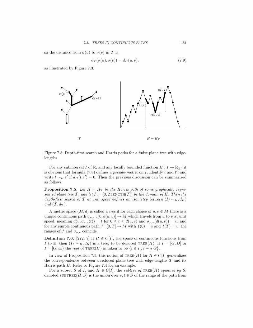
7.3. TREES IN CONTINUOUS PATHS 151

so the distance from σ(u) to σ(v) in T is

dT (σ(u), σ(v)) = dH(u, v), (7.9)

as illustrated by Figure 7.3.

uσ( )σ( )v

T

uH( )

H( )v

H( )u , v−

H = HT

Figure 7.3: Depth-first search and Harris paths for a finite plane tree with edge-lengths

For any subinterval I of R, and any locally bounded function H : I → R≥0 itis obvious that formula (7.8) defines a pseudo-metric on I . Identify t and t′, andwrite t ∼H t′ if dH(t, t′) = 0. Then the previous discussion can be summarizedas follows:

Proposition 7.5. Let H = HT be the Harris path of some graphically repre-sented plane tree T , and let I := [0, 2 length(T )] be the domain of H. Then thedepth-first search of T at unit speed defines an isometry between (I/∼H , dH )and (T , dT ).

A metric space (M,d) is called a tree if for each choice of u, v ∈M there is aunique continuous path σu,v : [0, d(u, v)]→M which travels from u to v at unitspeed, meaning d(u, σu,v(t)) = t for 0 ≤ t ≤ d(u, v) and σu,v(d(u, v)) = v, andfor any simple continuous path f : [0, T ]→M with f(0) = u and f(T ) = v, theranges of f and σu,v coincide.

Definition 7.6. [272, 7] If H ∈ C[I ], the space of continuous functions fromI to R, then (I/ ∼H , dH) is a tree, to be denoted tree(H). If I = [G,D] orI = [G,∞) the root of tree(H) is taken to be t ∈ I : t ∼H G.

In view of Proposition 7.5, this notion of tree(H) for H ∈ C[I ] generalizesthe correspondence between a reduced plane tree with edge-lengths T and itsHarris path H . Refer to Figure 7.4 for an example.

For a subset S of I , and H ∈ C[I ], the subtree of tree(H) spanned by S,denoted subtree(H ;S) is the union over s, t ∈ S of the range of the path from

152 Jim Pitman

s to t in tree(H), equipped with the tree metric dH . Let H ∈ C[I ] where I hasleft end 0. Assume for simplicity that 0 = H(0) ≤ H(t) for all t ∈ I . Let T1 > 0.Then subtree(H ; 0, T1) is isometric to a line segment of length H(T1). For0 < T1 < T2, let S1 be a time at which H attains its minumum on [T1, T2], andsuppose to avoid degenerate cases that H(S1) is strictly less than both H(T1)and H(T2). Then subtree(H ; 0, T1, T2) is isometric to a Y -shaped tree with 3edges of lengths H(S1), H(T1)−H(S1), and H(T2)−H(S1) respectively, whoseroot and leaves may be identified, in clockwise order from the bottom, as 0, T1

and T2 respectively, while the junction point is identified with S1. Continuingin this way, it is clear that for any finite sequence of sample times T1, . . . , Tn.the order and metric structure of subtree(H ; 0, T1, . . . , Tn) will be encodedby some plane tree. This can be made precise as follows, with some simplifyingassumptions to avoid annoying cases:

Lemma 7.7. Let X ∈ C[0, T ] and suppose X(t) ≥ X(0) = 0 for all t ∈ [0, T ].Let 0 < T1 < · · · < Tn ≤ T , and for 1 < m ≤ n let Si be a time in [Ti−1, Ti] atwhich X attains attains its minimum on [Ti−1, Ti], so

X(Si) := X[Ti−1, Ti],

and suppose that X(Si) < X(Ti−1)∧X(Ti). Then subtree(X ; 0, T1, . . . , Tn)is isometric to the unique reduced plane tree T whose 2n-step alternating excur-sion is

(0, X(T1), X(S2), X(T2), . . . , X(Sn), X(Tn), 0). (7.10)

Proof. It is easily seen that the assumptions on X and the Ti and Si implythat subtree(X ; 0, T1, . . . , Tn) has n leaves, that

0 < T1 < S2 < · · · < Tn

and that the lines joining consecutive points in the list

(0, X(0)), (T1, X(T1)), (S2, X(S2), (T2, X(T2)), . . . (Tn, X(Tn)). (7.11)

have slopes which are non-zero and alternate in sign. Let Y ∈ C[0, Tn] be thefunction whose graph is the broken-line joining the points (7.11). Then

subtree(X ; 0, T1, . . . , Tn)

is evidently isometric to tree(Y ), hence also to tree(H) where H is the uniquecontinuous time-change of Y whose graph has slopes of ±1. But this is the Harrispath whose 2n-step alternating excursion is (7.10), and the conclusion followsby Proposition 7.5.

Now consider the construction of tree(X) for a random function X ∈ C[I ],such as a Brownian path restricted to I . Intuitively, tree(X) should be regardedas a random metric space. Technically however, for purposes of measure theory,

7.4. BROWNIAN TREES AND EXCURSIONS 153

let us simply identify tree(X) with the random element dX of C[I × I ]. So for

instance tree(X)d= tree(Y ) means dX

d= dY which is the same as

(dX (u, v), u, v ∈ I)d= (dY (u, v), u, v ∈ I)

in the sense of equality of finite dimensional distributions. Now give the spaceof reduced plane trees the measurable structure it acquires when identified as asubset of C[0,∞) by using the Harris correspondence T ↔ HT . Here C[0, t] isregarded as a subset of C[0,∞), by stopping paths at time t. Then it is clearthat subtree(X ; 0, T1, . . . , Tn) may be regarded as a random reduced planetree for arbitrary I-valued random variables Ti defined on the same probabilityspace as a continuous path process X = (X(t), t ∈ I).

7.4. Brownian trees and excursions

Let B = (B(t), t ≥ 0) be a standard Brownian motion. An obvious geometricfeature of tree(B) is that this tree has a unique infinite branch, namely thedescending ladder set t : B(t) = B[0, t]. Except on an event with probabilityzero, this branch of tree(B), regarded as a subset of R≥0/∼B, is traversed atunit speed by the map `→ T`−, T` where

T` := inft : B(t) < −`.Let I` := [T`−, T`]. Then tree(B) is the union over ` ≥ 0 of subtree(B; I`),which is I` equipped with a tree structure isometric by a shift to tree(B[I`])on [0,∞), where

B[I`](t) := B((T`− + t) ∧ T`) (t ≥ 0).

Call the descending ladder set of B the floor line, to be identified with R≥0

by traversal at unit speed in tree(B), as above. Then tree(B) is identifiedby a forest of subtrees attached to the floor line, with a copy of tree(B[I`])attached to the point on the floor at distance ` from the root. Thus to de-scribe the structure of tree(B) it is enough to describe the forest of subtrees(tree(B[I`]), ` > 0).

Recall that if Bex is the standard excursion of length 1, then a Brownianexcursion Bex,t of length t can be defined by Brownian scaling. The distancefrom u to v in tree(Bex,t) is just

√t times the distance from u/t to v/t in Bex,

see Chapter 0.

Proposition 7.8. Let µ` := T`−T`−, which is the length of I`. Then the forestof Brownian subtrees (tree(B[I`]), ` > 0) is such that

(`, µ`,tree(B[I`])) : ` > 0, µ` > 0, (7.12)

is the set of points of a Poisson point process on R≥0×R≥0×C([0,∞)2) whoseintensity measure is

d`dt√

2πt3/2P(tree(Bex,t) ∈ dτ), (7.13)

154 Jim Pitman

where tree(Bex,t), the tree generated by a Brownian excursion of length t, isidentified by its distance function as a random element of C([0,∞)2).

Proof. According to the preceding discussion, tree(B[I`]) is a trivial treewith only one vertex unless T`− < T`, in which case tree(B[I`]) is the treegenerated by the excursion of B − B over the interval I`. So the statement ofthe proposition is just a push-forward of the Levy-Ito description of excursionsof B above B, which is reviewed in (0.17) .

To complete a description of the structure of tree(B), regarded as an infiniteforest of subtrees attached to the forest floor defined by the descending ladderset, it remains to describe tree(Bex). This is done by the following theorem.For ease of comparison with the work of Aldous [7], the theorem describestree(2Bex) = 2 tree(Bex), that is tree(Bex) with all distances doubled.

Theorem 7.9. Aldous [7]. Let U1, U2, . . . be a sequence of independent uniform[0, 1] variables, independent of Bex. For each n = 1, 2, . . ., let

Tn = subtree(2Bex; 0, U1, . . . , Un), (7.14)

regarded as a plane tree with edge-lengths, and let

Θn := length(Tn). (7.15)

Then (i)

Θn =√

2∑n

i=1 εi (7.16)

for a sequence of independent exponential(1) variables εi, and

Tn = ΘnBn,1 (7.17)

where (Θn, n ≥ 1) and (Bn,1, n ≥ 1) are independent, and Bn,1 has uniformdistribution on the set of planted binary plane trees whose total edge-length is 1,as defined by Lemma 7.4.

(ii) (Poisson line-breaking construction) The distribution of the se-quence of trees (Tn, n ≥ 1) is determined by the prescription (7.16) of theirlengths, and the following: for each n ≥ 1, conditionally given (Tj , 1 ≤ j ≤ n),the new segment of length Θn+1 − Θn, which is added to Tn to form Tn+1, isattached at a point of Tn picked independently of the new segment length ac-cording to the uniform distribution on edges of Tn, with equal probability to theleft or the right, independently of the point of attachment and the new segmentlength.

To rephrase the Poisson line-breaking construction: Let 0 < Θ1 < Θ2 < . . . bethe points of an inhomogenous Poisson process on R>0 of rate t dt. Break the line[0,∞) at points Θn. Grow trees Tn by letting T1 be a segment of length Θ1, thenfor n ≥ 2 attaching the segment (Θn−1,Θn] as a “twig” attached to a randompoint of the tree Tn−1 formed from the first n − 1 segments. Aldous [7, §4.3]

7.4. BROWNIAN TREES AND EXCURSIONS 155

discovered this result via weak convergence of combinatorially defined randomtrees, as indicated in Exercise 7.4.8 and Exercise 7.4.9 . This combinatorialapproach explains nicely why the Poisson line breaking construction of (Tn)implies (7.17), which is otherwise not very obvious. But Aldous’s argumentidentifying the laws of these trees with those embedded in Bex by (7.14) involvedan invariance principle implied by the invariance principle for conditioned Harriswalks Theorem 6.4 : Galton-Watson trees with Poisson offspring distribution orwith geometric offspring distribution converge in distribution to the same limit“continuum tree”; this limit was identified with tree(2Bex) in the geometriccase via the Harris bijection ( Exercise 7.4.15 ) while Poisson line-breakingarose in consideration of the Poisson offspring case ( Exercise 7.4.9 ). Le Gall[273] gave another proof of (7.17)-(7.16) based on calculations with Ito’s σ-finite excursion law. See also [275, Chapter 2]. A more elementary proof can begiven as follows, by relating Tn derived from Bex and U1, . . . , Un to the criticalbinary(0, 1

2 ) Galton-Watson tree with exponential edge-lengths conditioned tohave n leaves. Let Γr denote a gamma variable with parameter r > 0. Refer toFigure 7.5.

Lemma 7.10. Let T1 < T2 < . . . be the times of points of a Poisson processwith rate 1

2 on R≥0, assumed independent of B. Let [GT1 , DT1 ] be the excursioninterval of B −B straddling T1, and let

G := subtree(2B; GT1 , T1, . . . , TN) where N :=∞∑

i=1

1(Ti ≤ DT1) (7.18)

is the number of Ti which happen to fall in [GT1 , DT1 ]. Then(i) [399, 200] The tree G is a critical binary Galton-Watson tree, starting withone initial segment, in which each segment branches into either 0 or 2 segmentswith equal probability, and the segment lengths are independent exponential(1)variables.(ii) [355]

(G |N = n)d= Γ2n−1Bn,1 (7.19)

where Γ2n−1 is independent of Bn,1, which has uniform distribution on plantedbinary trees with n leaves and total edge-length 1.(iii) [355]

(G |N = n)d=√

2Γn− 12Tn (7.20)

where Γn− 12

is independent of Tn := subtree(2Bex; 0, U1, . . . , Un).

Proof. Part (i) is obtained by application of Lemmas 7.3 and 7.7, using thestrong Markov property of B at the times Ti, and the consequence of Williams’path decomposition of B at the time S1 ∈ [0, T1] when B(S1) = B[0, T1], that−B(S1) and B(T1)−B(S1) are independent exponential(1) variables. Part (ii)is then read from (7.5). As for (iii), it is clear by Brownian scaling that

(G |DT1 −GT1 = t,N = n)d=√t Tn.

156 Jim Pitman

From (7.13), the rate of excursions with length in dt which contain exactly nPoisson points is

1√2π

t−3/2dt e−t/2(t/2)n/n! = cntn− 1

2−1e−t/2dt.

This implies that (DT1 −GT1 |N = n)d= 2Γn− 1

2and the conclusion follows.

Proof of Theorem 7.9 This is a translation in terms of trees of an argumentgiven in [355] in terms of alternating walks: by consideration of moments andthe gamma duplication formula,

Γ2n−1d=√

2Γn−1/2

√

2Γ′n (7.21)

where Γ′n is assumed independent of Γn−1/2 with the same distribution as Γn.

Now (7.20) and (7.19) give√

2Γn− 12Tn

d=√

2Γn− 12

√

2Γ′n Bn,1.

It is easily argued that the common factor of√

2Γn− 12

can be cancelled [355,

Lemma 8] to yield (7.17) withd= instead of =. To check that the εi de-

fined implicitly by (7.17) are independent standard exponential, independentof (Bn,1, n ≥ 1), takes a bit more work. But this is essentially elementary, be-cause the conditional law of (Tj , 1 ≤ j ≤ n) given Tn is determined by a simpleprocess of random deletion of vertices and their incident edges. The same ele-mentary considerations yield (ii).

Alternative proof of Theorem 7.9(i) (Provided by J.-F. Le Gall.) LetT λ

1 < T λ2 < . . . be the times of points of a Poisson process with rate λ > 0,

independent of B, and

Gλ := subtree(2B; GT λ1, T λ

1 , . . . , TλNλ) where Nλ :=

∞∑

i=1

1(T λi ≤ DT λ

1).

By trivial extensions of (7.19)-(7.20),

(Gλ |N = n)d=

√

1

λΓn− 1

2Tn

and

(Gλ |N = n)d=

1√2λ

Γ2n−1Bn,1.

Thus, if F is any continuous function on the set of trees,

1

Γ(n− 12 )

∫ ∞

0

dt tn−3/2e−tE

[

F

(√

t

λTn

)]

=1

Γ(2n− 1)

∫ ∞

0

ds s2n−2e−sE

[

F

(s√2λBn,1

)]

.

7.4. BROWNIAN TREES AND EXCURSIONS 157

Make the changes of variables t = λt′, s =√

2λs′ and use the fact that

e−s√

2λ =

∫ ∞

0

dts√

2πt3e−s2/2te−λt.

It follows that

1

Γ(n− 12 )

∫ ∞

0

dt tn−3/2e−λtE

[

F(√

tTn

)]

=2n− 1

2

Γ(2n− 1)√

2π

∫ ∞

0

dt e−λtt−3/2

∫ ∞

0

ds s2n−1e−s2/2tE[F(sBn,1

)].

By injectivity of the Laplace transform

E

[

F(√

tTn

)]

=21−n

Γ(n)t−n

∫ ∞

0

ds s2n−1e−s2/2tE[F(sBn,1

)].

Take t = 1 to conclude.

Exercises

7.4.1. (Identification of paths in trees derived from continuous func-tions) Fix X ∈ C[I ]. Let t := u ∈ I : u ∼X t. Note that if t is the minimalelement of t, then t = u : X(u) = X[t, u] = X(t). For s, u ∈ I the unique pathfrom s to u at unit speed is determined by its range in I/∼X . This subset ofI/∼X is identified in the obvious way with a subset of [s, u], call it the segmentof tree(X) between s and u. This segment is the union of a falling segmentv ∈ [s, u] : X(v) = X[s, v], of length X(s) − X [s, u], and a rising segmentv ∈ [s, u] : X(v) = X [v, u] of length X(u)−X[s, u], these segments intersect-ing at the set of points v ∈ [s, u] : X(v) = X [s, u] where X attains its minimumon [s, u]. Each of these segments may also be regarded as a subset of I/ ∼X

which is isometrically parameterized by an interval. The falling segment is natu-rally parameterized by [X [s, u], X(s)], the rising segment by [X[s, u], X(t)], andthe whole segment by [0, dX(s, u)].

7.4.2. Let t be the equivalence class of t ∈ R≥0 equipped with the Browniantree metric dB . Deduce from the strong Markov property of B that

P( |t| = 1 or 2 or 3 for all t ≥ 0) = 1.

Check that t : t = 3 is a.s. equal to the countable set of all local minima of Bbesides those in the descending ladder set. See [324] for further analysis of localminima of B. Check that t : t = 2 is an uncountable set of Lebesgue measure0. This is essentially the skeleton of tree(B), as discussed in Chapter 10. Bothsets are a.s. dense in R≥0, both in the usual topology and in the topology oftree(B).

158 Jim Pitman

7.4.3. (Different processes with the same tree)

tree(B) = tree(B − 2B)d= tree(R3) (7.22)

where the first equality holds for every path B ∈ C[0,∞), and second equalityin distribution, read from [345] , assumes B is a standard Brownian motion andR3 is the 3-dimensional Bessel process. Hence for each fixed s,

(dB(s, s+ t), t ≥ 0)d= (R3(t), t ≥ 0)

but it seems there is no simple description of the joint law of dB(u, v) as bothu and v are allowed to vary. Note the implication of (7.22) that there is lossof information in passing from X to tree(X). Except if X(t) ≥ X(0) for allt ≥ 0, or if it is assumed that X has some particular distribution, the path ofX typically cannot be recovered from tree(X). Neither is the distribution ofX determined by that of tree(X).

7.4.4. (The filtration generated by the tree) Let Bt := σ(Bs, 0 ≤ s ≤ t)be the Brownian filtration, and let Rt be the σ-field generated by the restrictionof tree(B) to [0, t]. Check that Rt = σ(Rs, 0 ≤ s ≤ t) where Rt = dB(0, t) asin Exercise 7.4.3 , and hence that Bt is generated by Rt and B(t) where theconditional law of B(t) given Rt is uniform on [−R(t), 0], see [345].

7.4.5. (Processes generating Brownian trees) Show that for each proba-bility distribution F of a random variableM with values in [−∞, 0] there exists a

probability distribution on C[0,∞) for a processX such that tree(X)d= tree(B)

and X [0,∞)d= M . In particular, if M = −∞ then X

d= B, and if M = 0 then

Xd= R3. Describe the law of X by an explicit path decomposition in the case

M = m for some fixed m ∈ (−∞, 0), and hence give a construction of X corre-sponding to an arbitrary distribution of M .

7.4.6. (Trees derived from paths falling below their initial value) SeeFigure 7.4. Generalize Lemma 7.7 to the case when X may fall below its initialvalue, when the 2n-step alternating walk is not an excursion, by consideringexcursions of the alternating walk above its past minimum process. In general,the subtree of tree(X) spanned by 0, T1, . . . , Tn is determined by the 2n-stepalternating walk derived from the X(Ti) and intermediate X(Si), but not con-versely.

7.4.7. (Trees generated by bridges and meanders) Describe as explicitlyas possible the laws of the trees generated by each of the following processesindexed by [0, 1]: Brownian motion, Brownian bridge from 0 to x, Brownianmeander, Brownian meander from 0 to x. (Nasty descriptions in terms of alter-nating walks were given in [355]: there are much nicer descriptions, either in thestyle of the Poisson line-breaking construction, or in terms of forests of treesassociated with excursions).

7.4. BROWNIAN TREES AND EXCURSIONS 159

7.4.8. (Aldous’s proof of Theorem 7.9) Let UN have uniform distributionon the set of NN−1 rooted trees labeled by [N ]. For 1 ≤ n ≤ N let Un,N bethe subtree of UN spanned by the root and [n], let Tn,N be Un,N regarded asan ordered plane tree (e.g. by imposing a random order), and let Rn,N be thereduced plane tree derived from Tn,N by first giving each edge of Tn,N length

1/√N , then deleting all degree 2 vertices. Let Bn,N be the indicator of the

event that Rn,N is a planted binary tree with n leaves, and let Ln,N(i) be thelength of the ith branch of Rn,N , in order of depth first search. Check by directenumeration that for each fixed n, as N →∞,

(Ln,N(i), 1 ≤ i ≤ 2n− 1)1(Bn,N)d→ (Xi, 1 ≤ i ≤ 2n− 1)

where the right side is the sequence of lengths of branches of Tn in Theorem 7.9.Now deduce Theorem 7.9 from Theorem 6.4 . This method has proved effectivein characterizing other kinds of continuum random trees besides tree(Bex). See[20, 21].

7.4.9. (Combinatorial view of the line-breaking construction) (Aldous

[5, 6, 7]) Take (ξ(N)i , i ≥ 1) independent uniform on [N ]. Make a tree on [N ]

by declaring 1 to be the root and, for i = 2, 3, . . . , N , put an edge from i to

min(i− 1, ξ(N)i ). Apply a uniform random permutation to the vertex-labels [N ].

The resulting tree UN is uniform on allNN−1 rooted labeled trees, as in Exercise7.4.8 . (This fact is not obvious; it can be deduced from the Markov chain tree

theorem [292] applied to the Markov chain (ξ(N)i ); see also Definition 10.5 and

papers cited there). Let R(N)1 , R

(N)2 , . . . be the successive values of i for which

ξ(N)i ≤ i− 1. Show that

N−1(R(N)n , n ≥ 1)

d→ (Θn, n ≥ 1)

where the right side is defined by (7.16). Deduce that for fixed n, if we give length

N−1/2 to the edges of UN , then the subtrees comprised of the first R(N)n vertices

converge in distribution to Tn defined in the Poisson line-breaking construction(Theorem 7.9 (ii)).

7.4.10. (The Poisson line-breaking construction of Bex) Let (Tn)n=1,2,...

be the sequence of random trees defined by the Poisson line-breaking construc-tion, as in Theorem 7.9(ii), with Θn = length(Tn). Then there exists on thesame probability space an a.s. unique Brownian excursion Bex and a.s. uniqueindependent uniform Ui for 1 ≤ i ≤ n such that Tn is the subtree of tree(2Bex)spanned by 0, U1, . . . , Un. To be explicit, if Hn is the Harris path of Tn, then

Hn(2Θnu)→ 2Bex(u) (0 ≤ u ≤ 1) (7.23)

uniformly almost surely. Moreover, Un is the limiting fraction of times thatnew edges are added to the left of the nth edge that was added to the tree.

160 Jim Pitman

If (Wn,k , 0 ≤ k ≤ 2n) is the alternating excursion associated with Tn, then for1 ≤ m ≤ n

Wn,2m−1 = 2Bex(Un,m) (1 ≤ m ≤ n) (7.24)

where Un,m is the mth smallest among U1, . . . , Un, and for 1 ≤ m ≤ n− 1

Wn,2m = 2Bex[Un,m, Un,m+1]. (7.25)

7.4.11. (An urn-scheme construction of Bex) Let (Sn)n=1,2,... be the se-quence of shapes of the random trees (Tn)n=1,2,... defined by the Poisson line-breaking construction, as in Theorem 7.9 (ii). So Sn ∈ binaryn, the set ofn-leaf combinatorial planted binary plane trees. Let S[n] be Sn with its n leaveslabeled by [n], according to their order of addition in the growth process. SoS[n] ∈ binary[n], the set of n-leaf binary plane trees with leaves labeled by [n],with |binary[n]| = n!|binaryn|. Show that both (Sn)n=1,2,... and (S[n])n=1,2,...

are Markov chains, and describe their transition probabilities. Check in par-ticular that given S[n], the next tree S[n+1] is equally likely to be any of the2(2n − 1) trees which can be grown from S[n] by replacing one of the 2n − 1edges of S[n], say the edge a → b, by two edges and a new internal vertex c toform a→ c→ b, then attaching the leaf labeled (n+ 1) by an edge (n+ 1)→ c,on one side or the other of a → c → b. Note the byproduct of this argumentthat for n = 1, 2, . . .

|binary[n+1]| = 2n(1× 3× 5× · · · × (2n− 1)) =

(2n

n

)

n!, (7.26)

and hence:

|binaryn+1| =|binary[n+1]|

(n+ 1)!=

1

n+ 1

(2n

n

)

, (7.27)

which is the nth Catalan number Cn [407, Exercise 6.19]. Thus, a sequenceof trees distributed like (S[n])n=1,2,... can be grown by a simple urn schemeconstruction, similar to the Chinese Restaurant Process described in Chapter 3,and Sn is derived from S[n] by ignoring the labelling by [n]. Deduce from (7.23)

and Θn ∼√

2n a.s. that if HSnis the Harris path of Sn, then

HSn(2(2n− 1)u)√

2n→ 2Bex(u) (0 ≤ u ≤ 1) (7.28)

uniformly almost surely, where Bex is the same Brownian excursion as thatderived similarly from (Tn)n=1,2,... by (7.23). As a check on the normalization,

the weaker form of (7.28) withd→ instead of almost sure convergence is the

instance of Aldous’s result Theorem 6.4 for binary branching, due to Gutjahr-Pflug [181]. See also [261, 376, 418, 419, 247] for various other models for randomgrowth of binary trees.

7.4. BROWNIAN TREES AND EXCURSIONS 161

7.4.12. (Independent self-similar growth of subtrees) The combinatorialtree growth process (Sn)n=1,2,... embedded in Bex as in the previous exercisehas the following remarkable property. Suppose that e is one of the 2m − 1edges of Sm, for some fixed m. Then for each n ≥ m there is an obvious wayto identify a subtree of Sn formed by e and all its offshoots, which will be acombinatorial planted binary plane tree. If this sequence of offshoots grows byaddition of leaves at random times m < N1(e) < N2(e) < . . . say, then Nk(e)increases to∞ almost surely, and the sequence of offshoots of e, watched only atthe times m,N1(e), N2(e), . . ., and re-indexed by 1, 2, . . ., defines a tree growthprocess, call it the sub-process generated by e, which has the same distributionas the original growth process. Moreover, as e varies over the 2m − 1 edges ofTm, these 2m− 1 sub-processes are independent.

7.4.13. (Dirichlet distribution of proportions of subtrees) Continuingthe previous exercise, for each fixed m, as n varies over n ≥ m, the process ofallocation of new leaves to the offshoots of edges e of Sm is equivalent to Polya’surn scheme with 2m − 1 initial balls of different colors, governed by samplingwith double replacement. Hence, by Exercise 2.2.2 , as n→∞, the proportionsof edges in the 2m+ 1 subtrees converge almost surely to a random vector withthe symmetric Dirichlet distribution with 2m+ 1 parameters equal to 1

2 . Notethat the same is true of proportions of leaves, since a planted plane binary treewith 2n−1 edges has n leaves. Both processes may be regarded as developmentsof the Blackwell-MacQueen urn scheme [68, 350].

7.4.14. (An urn-scheme construction of Bbr) Recall that S[n] is Sn withthe leaves labeled by their order of appearance in the urn-scheme constructionof Bex. Let σ(t), 0 ≤ t ≤ 2(2n − 1) be the usual depth-first search of Sn, anddefine the trunk of Sn to be the path from its root to the vertex labeled 1in S[n]. For 0 ≤ u ≤ 1 let Rn(u) be the distance from σ(2(2n − 1)u) to thetrunk as measured along edges of Sn, and let Sn(u) be Rn(u) with a sign ±1according to whether σ(2(2n−1)u) is to the left or the right of the trunk. Then,as companions to (7.28), there is almost sure convergence of Sn/

√2n to 2Bbr

and Rn/√

2n to 2|Bbr|, where Bbr can be derived as a measurable functionof Bex and the independent uniform variable U1 which is the limiting fractionof leaves of S[n] which are to the left of leaf 1 at the top of the trunk. Thisis a variant of transformations between Bex and Bbr discussed in [53]. Notehow the uniform location of 1 among the leaves implies Levy’s theorem that∫ 1

01(Bbr

u > 0)du has uniform [0, 1] distribution. See Knight [257] and Kallenberg[229] for generalizations to bridges with exchangeable increments, and relatedresults.

7.4.15. (Weak convergence of conditioned Galton-Watson trees) Con-sider a critical Galton-Watson branching process with offspring variance σ2.Write TN for this tree conditioned to have exactly N vertices, with each edgegiven length N−1/2. Aldous [7] gave a sense, implied by Theorem Theorem 6.4,in which TN converges in distribution to tree(2σ−1Bex). Check the scaling con-stant 2/σ is consistent with what is known by other methods in the following

162 Jim Pitman

three special cases.

• (a) For Poisson(1) offspring distribution. Here shape(TN ) is obtained byrandomly ordering the branches of the uniform tree UN of Exercise 7.4.8.

• (b) For geometric(1/2) distribution. Here shape(TN ) is uniform on allcombinatorial plane trees, which by the Harris correspondence are bijectivewith simple walk-excursions of length 2N .

• (c) For binary offspring distribution, i.e. uniform on 0 and 2. Now shape(TN ),for N = 2M − 1, is uniform on binary plane trees with M leaves, as inExercise 7.4.11 .

Notes and comments

Neveu [320, 321] introduced a notion of marked trees, used also by Le Gall [273],which is essentially equivalent to the notion of plane trees considered here. Thestructure of subtree(B; T0, T1, . . . , TN) for suitable random T0, . . . , TN , wasfirst considered in [323, 324], where it was shown that some Ti defined in terms ofsuccessive upcrossings and downcrossings by B induce a critical binary Galton-Watson tree. Aldous ([7] and subsequent papers) calls tree(2Bex) the Browniancontinuum random tree (CRT). See also [8] regarding recursive self-similarityproperties of tree(2Bex), and random triangulations. Kersting [246] discussessymmetry properties of binary branching trees implicit in Aldous’s descriptionof tree(2Bex).

7.5. Plane forests with edge-lengths

The idea of this section is to consider the tree

F := subtree(B; 0, T1, T2, . . .)

for B a Brownian motion, and suitable increasing sequences of random times Ti,called sampling times. To avoid uninteresting complications, it will be assumedthroughout that

0 = T0 < T1 < T2 < · · · < Tn ↑ ∞ (7.29)

almost surely. The assumption that Tn ↑ ∞ implies infnB(Tn) = −∞, whichmeans that F will contain the entire infinite floor line of tree(B) correspondingto the descending ladder set of B. Thus F may be regarded as a random locallyfinite plane forest, that is an infinite sequence of plane trees, each with a finitenumber of edges of finite length, with the roots of these trees located at somestrictly increasing sequence of points

0 < L1 < L2 < · · · < Lk ↑ ∞

where Lk is the common value of −B(t) for t in the kth excursion interval ofB −B that contains at least one Ti. Moreover, it is clear that with probability

7.5. PLANE FORESTS WITH EDGE-LENGTHS 163

one, each of the tree components of F will be a planted binary plane tree, andthat F can be identified graphically when convenient as a subset of R2. Thedefinition of Harris paths is extended to such forests (including also subforestswith only a finite number of trees) as follows. If F0 is the trivial forest with notrees, then HF0 is the trivial path, starting at 0, with constant slope −1. Fora non-trivial locally finite plane forest F , let HF(·) be defined by inserting theHarris paths of the component subtrees of F into the trivial path, in such a waythat if Ti is the tree component of F whose root is located at `i, and

Ti := `i +∑

j<i

2length(Tj) = inft : HF (t) = −`i

thenHF (Ti + t) = HTi

(t) (0 ≤ t ≤ 2length(Ti))

and HF (·) is continuous with slope −1 on each of the intervals

(`i−1 +∑

j<i

2length(Ti), `i +∑

j<i

2length(Ti))

where `0 = 0 and `k =∞ if F has fewer than k trees. Refer to Figure 7.6.

Intuitively, for reasonable families of sampling times (Tmi , i ≥ 1) whose inter-

vals become small as m→∞, we expect the forests

Fm = subtree(B; 0, Tm1 , Tm

2 , . . .)

to converge to tree(B). It will be shown in Sections 7.6 and 7.7 that thereare two particular choices of sampling sequences for which the forest-valuedprocesses (Fm) have interesting autonomous descriptions, given in Definitions7.16 and 7.21. To get started, note that various results presented in terms oftrees in the previous sections now have analogs in terms of forests. For instance,here are the forest analogs of Proposition 7.5, Lemma 7.7, Definition 7.2, andLemma 7.3.

Proposition 7.11. Let H = HF be the Harris path of some locally finite graph-ically represented plane forest F . Then the depth-first search of F at unit speedinduces a bijection from [0,∞)/∼H to F whereby the metric space [0,∞)/∼H

is isometric to (F , dF ).

Lemma 7.12. For m = 1, 2, . . . let Sm be a time in [Tm−1, Tm] at which Battains its minimum on [Tm−1, Tm] so

B(Sm) := B[Tm−1, Tm].

Then subtree(B; 0, T1, T2, . . .) is isometric to the unique locally finite forestdefined by a sequence of reduced plane trees attached to points along a floorline, whose Harris path HF (·) is a time-change with alternating slopes ±1 ofthe broken line joining the sequence of points

(0, 0), (S1, B(S1)), (T1, B(T1), (S2, B(S2)), (T2, B(T2)), . . . .

164 Jim Pitman

The notation F(B; 0, T1, T2, . . .) may now be used either for the locallyfinite reduced plane forest defined by the Lemma, or for the isometric infinitesubtree of tree(B) spanned by the set of points 0, T1, T2, . . ..Definition 7.13. A binary(λ, µ) forest is a planted binary plane forest F withedge-lengths whose trees are a sequence of independent and identically dis-tributed binary(λ, µ) trees, which are rooted at the set of points of an indepen-dent Poisson process on [0,∞) with rate µ− λ.

Lemma 7.14. A locally finite forest F of reduced plane trees is a binary(λ, µ)forest if and only if the succession of falls and rises of its Harris path HF is asequence of independent exponential variables, with exponential(µ+λ) rises andexponential(µ− λ) falls.

Proof. This follows from Lemma 7.3 and the fact that the exponential rateµ − λ of the spacings between trees in a binary(λ, µ) forest is by definitionthe same as the rate of the exponential falls of the alternating random walkused to construct the binary(λ, µ) tree. This means that the absolute value ofthe overshoot of the alternating exponential walk used to make the ith tree ofthe forest has exactly the correct exponential(µ − λ) distribution to make thespacing on the forest floor between the ith and (i+ 1)th trees.

Note how the description of the binary(λ, µ) forest is simpler than the corre-sponding description of the binary(λ, µ) tree by stopping the associated alter-nating random walk when it first steps negative.

7.6. Sampling at downcrossing times

Throughout this section, let B denote a standard Brownian motion, with B0 = 0.Following [324], consider for each θ > 0 the sequence of downcrossing timesDθ

m defined inductively as follows. Let Dθ0 = 0. Given that Dθ

m has beendefined, let

Uθm+1 := inft : Bt −B[Dθ

m, t] = θ−1,Dθ

m+1 := inft : B[Uθm+1, t]−Bt = θ−1. (7.30)

In words, Uθm+1 is the first time after Dθ

m that B completes an upcrossing ofsome interval of length θ−1, and Dθ

m+1 is the next time after U θm+1 that B

completes a down-crossing of some interval of length θ−1. By construction, theDθ

m are stopping times relative to the filtration of B, and B[Dθm, D

θm+1) =

B(Uθm+1)−θ−1. The level θ−1 is chosen so that θ is the rate, per unit increment

of −B, of the Poisson process of excursions of B −B which reach level θ−1.

Theorem 7.15. [324] For each fixed θ > 0,

FθB := F(B; 0, Dθ

1, Dθ2 , . . .)

is a binary(0, θ) forest of critical binary trees, in which segments are attachedto the floor by a Poisson process with rate θ, each segment has either 0 or

7.6. SAMPLING AT DOWNCROSSING TIMES 165

2 children with equal probability, and the lengths of segments are independentexponential(2θ) variables.

Proof. This can be read from the Poisson character of Brownian excursions,as shown in [324].

Two alternative viewpoints are useful. Firstly, the forest F θB may be regarded

as an infinite subtree of tree(B). From this perspective, the process (F θB)θ≥0

is a forest growth process, meaning that FλB can be identified as a subforest of

FµB whenever λ < µ. Secondly, to regard (Fθ

B)θ≥0 as a forest-valued process, thespace of locally-finite plane forests is identified as a subset of C[0,∞) via theHarris correspondence, and C[0,∞) is given the topology of uniform convergenceon compacts. The forest growth process (Fθ

B)θ≥0 has the special property thatfor each fixed λ > 0 the entire path (Fθ

B)0<θ≤λ can be recovered as a measurable

function of FλB . Indeed, as h increases, the process (F1/h

B )h>0 is the deterministicprocess of continuous erasure of tips, described by Neveu [321]. The law of thewhole forest growth process (Fθ

B)θ≥0 is determined by this observation and thedistribution of Fθ

B for fixed θ given by Theorem 7.15. The following definitionis suggested by these considerations and the work of Abraham [1, p. 382]:

Definition 7.16. A tip-growth process is a time inhomogeneous forest-valuedMarkov process with continuous paths, (Fθ)θ≥0, which starts at the empty forestat time θ = 0, and develops as follows:

• at each time θ, along each side of each edge of F θ, new tips of length 0are born according to a Poisson process with unit rate per unit length ofside per unit time;

• each tip that is alive at time θ is growing away from the root of its tree atspeed θ−2.

In the description of these Poisson rates, each of the subintervals of [0,∞)between the roots of trees of Fθ, including the interval before the first root, isregarded as an edge of Fθ with only one (upward) side from which new tipscan sprout and then grow into larger trees by addition of further tips. All otheredges of Fθ are regarded as having two sides.

Now there is the following refinement of Theorem 7.15:

Corollary 7.17. The forest-valued process (F θB)θ≥0 is a tip-growth process such

that FθB is a binary(0, θ) forest of critical binary trees. Conversely, if (F θ)θ≥0 is

such a forest growth process, there exists on the same probability space a uniqueBrownian motion B such that (Fθ)θ≥0 = (Fθ

B)θ≥0 almost surely. Explicitly,

B(t) = limθ→∞

Hθ(θt) (0 ≤ t <∞) (7.31)

where Hθ is the Harris path associated with Fθ, and the convergence holds inC[0,∞) almost surely.

166 Jim Pitman

Proof. The first sentence can be read from the previous discussion, and Ito’sexcursion theory. See Abraham [1, p. 382], where the tip-growth evolution isdescribed just for a single tree born at time θ which is then destined to haveultimate maximum height θ−1. The proof of the converse is similar to the proofof the converse in Exercise 7.7.4 .See also Abraham [1, V], where a variant of (7.31) is given for recovery of asingle excursion of B from a growing family of subtrees.

To amplify the Brownian interpretation of the tip-growth process, a tip bornat time θ will have grown into a branch of total length θ−1−φ−1 at a subsequenttime φ, by which time other tips may have started growing from this branchaccording to the Poisson process of birth of new tips. Thus each tip born attime θ anticipates a local maximum of B at a level exactly θ−1 higher than thelevel where the tip is born. See also Abraham [1] for further discussion.

7.7. Sampling at Poisson times

Let N be a homogeneous Poisson point process on (0,∞)2, with unit rate perunit area, assumed independent of the Brownian motion B. Consider the forest-valued process

FθN,B := F(B; 0, T θ

1 , Tθ2 , . . .)

generated by sampling B at the times

T θm := inft : N([0, t]× [0, 1

2θ2]) = m. (7.32)

To match the parameterizations of the two forest growth processes describedby Corollary 7.17 and Theorem 7.18, the level 1

2θ2 is chosen in (7.32) because

θ is the rate per unit local time of Brownian excursions which contain at leastone point of N below 1

2θ2. It follows that sample times T θ

m and Dθm have the

same mean 2/θ2, but these sample times have different variances. From thedefinition (7.30), the distribution of Dθ

1 is that of the sum of two independentcopies of the first hitting time of θ−1 by |B|, whereas the distribution of T θ

1 isexponential( 1

2θ2).

Theorem 7.18. [399, §6.2],[200] For each fixed θ > 0, the infinite subtree FθN,B

of the Brownian tree, obtained by sampling at Poisson times with rate 12θ

2, is abinary(0, θ) forest of critical binary trees, hence identical in law to F θ

B obtainedby sampling at downcrossings of size θ−1.

Proof. In view of Lemma 7.3, and the coding of forests by alternating walksdiscussed in Section 7.1, part (i) follows from the strong Markov property of

B at the times T θm, and Williams’ decomposition of B at the time S

(θ)1 of its

minimum before the exponential( 12θ

2) time T θ1 , whereby the random variables

B(Sθ1 ) := B(T θ

1 ) and B(T θ1 )−B(Sθ

1 ) are independent exponential(θ) variables.See also [399, §6.2], [355], [200] for variations of this argument.

7.7. SAMPLING AT POISSON TIMES 167

The parallel between Theorems 7.15 and 7.18 invites an analysis of the for-est growth process (Fθ

N,B)θ≥0 analogous to Corollary 7.17. An analog for thePoisson-sampled Brownian forest of Neveu’s process of erasure of tips is pro-vided by the next lemma, which follows immediately from standard propertiesof Poisson processes:

Lemma 7.19. For Fθ := FθN,B, the forest growth process is such that for each

0 < λ < µ, conditionally given Fµ, the forest Fλ is derived from Fµ by takingthe subforest of Fµ spanned by a random set of leaves of Fµ picked by a processof independent Bernoulli trials so for each i the ith leaf of Fµ in order of depth-first search is put in the spanning set with probability λ2/µ2.

This lemma and Theorem 7.18 determine the joint distribution of Fλ andFµ for arbitrary 0 ≤ λ < µ. This in turn determines the distribution of thewhole forest-growth process (Fθ)θ≥0, because it turns out to be Markovian. ThisMarkov property is not obvious, but a consequence of the following theorem.

To formulate the theorem, consider more generally a forest growth process(Fθ)θ≥0. Then for each choice of λ and µ with 0 ≤ λ ≤ µ, there exists a jointgraphical representation of Fλ and Fµ, as unions of line segments in the plane,such that Fλ is contained in Fµ. The set-theoretic difference Fµ − Fλ is thena disjoint union of subtrees of Fµ, each attached to some point on the sides ofFλ. For each of these subtrees, if it is attached to point x on the side of Fλ, andx is reached at time t(x) in the depth-first search of Fλ at unit speed, let thesubtree be detached from x and then rerooted on an empty forest floor [0,∞)at distance t(x) from 0.

The result is a new forest Fλ→µ, the forest of innovations or increments inthe forest growth process between times λ and µ. Now Fλ can be understoodas derived from the earlier forest Fµ and the forest of innovations Fλ→µ by anoperation of composition of Fλ and Fλ→µ, whereby the forest Fλ→µ is wrappedaround the sides of Fλ according to the depth-first search of Fλ at unit speed.Refer to Figure 7.7.

In terms of Harris paths, this means that the Harris path of Fµ is obtainedby inserting excursions defined by the Harris path of Fλ→µ into the Harris pathof Fλ at appropriate times. Two precedents for construction of processes bythis kind of insertion of excursions are the approximation of continuous timecountable state space Markov chains with instantaneous states [157], and theconstruction of downwards skip free processes driven by a subordinator [3]. Saythat a forest growth process (Fθ)θ≥0 has independent growth increments if foreach choice of times 0 = θ0 < θ1 < . . . < θn the increments Fθi−1→θi for1 ≤ i ≤ n are independent. Obviously, such a process is Markovian.

Theorem 7.20. [364] The Poisson-sampled Brownian forest (F θ)θ≥0 := (FθN,B)θ≥0

has independent growth increments, such that for each 0 ≤ λ < µ the forestof increments Fλ→µ is a binary(λ, µ) forest as in Definition 7.13. Moreover,(Fθ)θ≥0 is a twig-growth process, in the sense of the following definition.

Proof. This is deferred to the next Section 7.8.

168 Jim Pitman

Definition 7.21. cf. [5, p. 2, Process 2] A twig-growth process is a forest-valuedprocess (Fθ)θ≥0 such that, with the conventions discussed in Definition 7.16

• (Fθ)θ≥0 is a time inhomogeneous forest-valued Markov process with cadlagpaths, which starts as the empty forest at time θ = 0, and develops as fol-lows:

• at each time θ, along each side of each edge of F θ, twigs are attached tothat side according to a Poisson process with rate 1 per unit length of sideper unit time;

• given that a twig is attached to a point x on some side of F θ at time θ,the length of that twig has exponential(2θ) distribution.

Note that the rule for generation of points of attachment of new twigs in thetwig-growth process is identical to the rule for generation of new tips in thetip-growth process, according to Definition 7.16. But a tip that appears in thetip-growth process at time θ grows continuously to an ultimate length of θ−1,whereas a twig appearing at time θ in the twig-growth process grows instanta-neously and hence discontinuously to its final length, which is exponential withmean 1

2θ−1.

The twig growth process is most easily motivated as the “local” (that is,near the root) variant of a process implicit in the Poisson line-breaking con-struction. To outline this connection, recall the description below Theorem 7.9in terms of the inhomogenous Poisson process (Θi), with intensity tdt. Fix anedge segment I of some initially fixed length ε near the root in some Tn, andconsider how twigs are subsequently attached to points within that edge seg-ment. The ith such twig to be attached will be an interval of [0,∞) of the form[Θi, Θi + η(Θi)), where by Poisson thinning the (Θi) are the points of a Pois-son process with constant rate ε, and η(θ) is approximately exponential(θ) forlarge θ. Now imagine traversing [0,∞) at speed 2/ε, so that at time θ we are atposition 2θ/ε, Then the times of attachments of twigs to segment I will be ap-proximately Poisson, rate 2, and a segment attached at time θ will have lengthwith approximately exponential(2θ/ε) distribution. Now magnify all lengths bya factor 1/ε; in particular the initial edge of T1 now has length of order 1/ε.The above definition of the twig growth process is identical to the ε → 0 limitof this process, except for the following subtle difference: Part of our conventionabout forests is that the floor has only one side, while the edges of trees havetwo sides. But in the above limiting argument, the floor arises as a limit of atree edge, so needs to be given two sides. Exercise 7.7.6 develops this variationof the twig growth process, as originally defined by Aldous [5, p. 2, Process 2].

Exercises

7.7.1. Explain why a twig-growth process has independent growth increments.

7.7.2. Show that the first sentence of Theorem 7.20 implies the second one.

7.7. SAMPLING AT POISSON TIMES 169

7.7.3. (Problem) Theorem 7.20 implies that if (Fθtwig)θ≥0 is a twig-growth

process, then

Fθtwig is a binary(0, θ) forest of critical binary trees. (7.33)

It must be possible to check this by showing that this family of laws satisfies asystem of Kolmogorov forwards equations generated by the jump-hold descrip-tion of suitable restrictions of the twig-growth process. Formulate the appropri-ate equations, and show they are uniquely solved by this family of laws. Thatdone, it should be possible to complete a proof of Theorem 7.20 by a repetitionof the argument to show that the forest of increments between times λ and µ isa binary(λ, µ) forest.

7.7.4. (Recovery of B and N from a twig-growth process) This corollaryof Theorem 7.20 sharpens the results of Aldous [5], who used the twig-growthprocess to construct a random metric space isometrically equivalent to the self-similar Brownian tree, without reference to Brownian motion. Given a twig-growth process (Fθ)θ≥0, there exists on the same probability space a uniquePoisson process N and a unique Brownian motion B such that (F θ)θ≥0 =(Fθ

N,B)θ≥0 almost surely. Moreover, both N and B are almost surely unique,

and they are independent. In particular, B(·) is recovered from (F θ)θ≥0 just asin (7.31), and for each fixed m and λ > 0 the time T λ

m of the mth point of N in(0,∞)× [0, 1

2λ2] is recovered as the almost sure limit

T λm = lim

θ→∞S(λ,θ)

m /θ (7.34)

where S(λ,θ)m is the a.s. unique time s at which the Harris path of Fθ has a local

maximum at the height above the forest floor of the mth leaf of Fλ.

7.7.5. (Almost sure identity of the two infinite forests) For each fixedλ > 0 and each fixed ` > 0, there exists an almost surely finite random timeΘ(λ, `) such that

FλB [0, `] ⊂ Fθ

N,B and FλN,B[0, `] ⊂ Fθ

B for all θ ≥ Θ(λ, `) (7.35)

where F [0, `], the restriction of F to [0, `], is obtained by clear-cutting all treesof F whose roots fall in (`,∞).

7.7.6. (The self-similar CRT) Write B± for two copies (B+(t), t ≥ 0) and(B−(t), t ≥ 0) of standard Brownian motion, or equivalently the two sided mo-tion (B±(t),−∞, t <∞). Interpret tree(B±) as the two-sided forest, in whichB+ defines trees “upwards” from the floor [0,∞) while B− defines trees “down-wards” from the floor [0,∞). This is the limit tree suggested by the discussionof Definition 7.21. The scaled tree tree(2B±), or equivalently the scaled treetree(2R±

3 ) for two-sided Bessel(3) R±3 (cf. Exercise 7.4.3 ) is what Aldous [12]

called the self-similar CRT.(a) Extend Bex to all real t by interpreting Bex(t) = Bex(t mod 1). Observe

that as ε ↓ 0

(ε−1/2Bex(εt),−∞ < t <∞)d→ (R±

3 (t),−∞ < t <∞).

170 Jim Pitman

In this sense, two-sided Bessel(3) is the “local limit” of Brownian excursion near0.

(b) Combine the discussion of Definition 7.21 with Exercise 7.4.9 to argueinformally the following. Let UN be uniform on all NN−1 rooted labeled trees.Let k(N)→ 0, k(N)/N−1/2 →∞. Give length k(N) to each edge of UN . ThenUN converges in distribution to the self-similar CRT [12].

7.7.7. (The forest generated by Brownian motion with drift.) For δ ∈ R

let Bδ(t) := B(t) + δt, t ≥ 0. This exercise is a reformulation in terms of treesof David Williams’ path decompositions for Bδ , and their explanation in termsof the transformation from Bδ to Bδ − 2Bδ. See [436, 270] for background.

• the distribution of tree(Bδ) depends only on |δ|.• for δ > 0 the process tree(Bδ) is independent of −Bδ(∞), which has

exponential(2δ) distribution.• for ` > 0 let T δ

` denote the subtree of tree(Bδ) which is attached to itsinfinite branch at distance ` from 0, let µδ

` be the mass of T δ` , meaning

the length of the corresponding excursion interval of Bδ, and identify T δ`

with the isometric tree structure on [0, µδ` ]. Then

(`, µδ` , T δ

` ) : µδ` > 0

is the set of points of a Poisson process with intensity

d`e−12 δ2t dt√

2πt3/2P(tree(Bex,t) ∈ dτ).

Notes and comments

Special thanks to David Aldous for help in writing this section, which bridgesthe gap between descriptions of the Brownian forest given by Neveu-Pitman[323, 324] and Aldous’s construction of a self-similar CRT by the twig growthprocess.

7.8. Path decompositions

Definition 7.22. Given a path B and sampling times T1, T2, . . ., the alternatinglower envelope of B derived from T1, T2, . . . is the process with locally boundedvariation At := At(B, T1, T2, . . .) defined as follows:

At =

B[Tm, t] if t ∈ [Tm, Sm+1]B[t, Tm+1] if t ∈ [Sm+1, Tm+1]

(7.36)

where T0 = 0 and Sm+1 is the time in [Tm, Tm+1] at which B attains its min-imum on that interval. Note that Sm+1 = Tm or Sm+1 = Tm+1 may occurhere, causing degeneracy in the sequel. We therefore assume throughout that B

7.8. PATH DECOMPOSITIONS 171

and Tm are such that this does not happen, as is the case almost surely in ourapplications to Poisson-sampled Brownian paths.

Call the reflected process Rt := Bt − At ≥ 0 the height of B above itsalternating lower envelope derived from T1, T2, . . . Define a random sign processσt, with σt = −1 if t is in one of the intervals [Tm, Sm+1) when A is decreasing,and σt = +1 if t is in one of the intervals [Sm+1, Tm+1) when A is increasing,so the process

Lt :=

∫ t

0

σsdAs

is a continuous increasing process, call it the increasing process derived from Band T1, T2, . . ..

Lemma 7.23. For an arbitrary continuous path B with inf tBt = −∞, let F bethe forest derived from B by sampling at some finite or infinite increasing se-quence of times Tm, and let F ′′ be the forest derived from B by sampling at somesequence of times T ′′

m, where T ′′m = Tm ∪ T ′

m for some finite or infiniteincreasing sequence of times T ′

m. Let At = At(B, T1, T2, . . .) be the alternatinglower envelope of B induced by the Tm, let Lt = Lt(B, T1, T2, . . .) be the in-creasing process derived from B and the Tm. Then the forest of innovationsgrown onto F to form F ′′ is identical to the forest derived from B − A − L bysampling at the times T ′

m.Proof. This is left as an exercise.

Theorem 7.20 now follows easily from the construction of the forest growthprocess (Fθ)θ≥0 by Poisson sampling of B, the previous Lemma, and the fol-lowing lemma.

Lemma 7.24. For δ ≥ 0 let P−δ govern (Bt, t ≥ 0) as a Brownian motion withdrift −δ, meaning that the P−δ distribution of (Bt, t ≥ 0) is the P0 distributionof (Bt − δt, t ≥ 0). Let P−δ also govern T θ

m for m = 1, 2, . . . as the points of aPoisson process with rate 1

2θ2 which is independent of B. For m = 1, 2, . . . let

F θm := B(T θ

m−1)− B(Sθm) be the mth fall and Hθ

m := B(T θm) − B(Sθ

m) the mthrise of the alternating walk defined by the values B(T θ

m) and the intermediateminima B(Sθ

m). Then under P−δ for each −δ ≤ 0:(i) the random variables F θ

m and Hθm are independent, with

F θm

d= exponential(

√

θ2 + δ2 − δ) (7.37)

Hθm

d= exponential(

√

θ2 + δ2 + δ). (7.38)

(ii) Let Lθ be the increasing process and Aθ the alternating lower envelope de-rived from B and the sample times T θ

m. Then the process B − Aθ − Lθ is aBrownian motion with drift −

√θ2 + δ2. Equivalently, B − Aθ is a Brownian

motion with drift −√θ2 + δ2 on (0,∞) and simple reflection at 0.

(iii) The Brownian motion B−Aθ−Lθ with drift −√θ2 + δ2 is independent of the

bivariate sequence of falls and rises (F θm, H

θm)m=1,2,..., hence also independent

of the Poisson-sampled Brownian forest F θN,B which they encode.

172 Jim Pitman

Proof. The independence assertions in (i), and the exponential form of thedistributions of the falls and rises follow from Williams’ path decomposition ofB at the time Sθ

1 of its minimum on the interval [0, T θ1 ], and repeated application

of the strong Markov property of B at the times T θm. See [436, 178]. Using

independence of F θ1 and Hθ

1 , the parameters of the exponential distributionsare easily derived from the the first two moments of B(T θ

1 ).

Or see [73]. Also according to Williams [436], conditionally given F(θ)1 = f

and H(θ)1 = h, the fragments of the path of B on the intervals [0, Sθ

1 ] and[Sθ

1 , Tθ1 ] are independent, the first fragment is distributed like a Brownian motion

with drift −√θ2 + δ2, started at 0 and run until it first hits −f , while the

second fragment reversed is like a Brownian motion with the same negativedrift started at h − f and run until it first hits −f . It follows that with thesame conditioning, the two reflected path fragments (Bt − Aθ

t , 0 ≤ t ≤ Sθ1) and

(BSθ1+u −Aθ

Sθ1+u

, 0 ≤ u ≤ T θ1 − Sθ

1) are independent, the first fragment being a

reflected BM with drift −√θ2 + δ2, run until its local time at 0 reaches f , and

the second fragment reversed being a reflected BM with drift −√θ2 + δ2, run

until its local time at 0 reaches h. But from this description, and the well-knownreversibility of a one-dimensional diffusion stopped at an inverse local time, stillconditioning on F θ

1 = f and Hθ1 = h, the process (Bt − Aθ

t , 0 ≤ t ≤ T θ1 ) is

identified as a reflected BM with drift −√θ2 + δ2 run until its local time at 0

first reaches f + h. Now by repeated use of this argument, the entire process(Bt − Aθ

t , t ≥ 0) conditional on all the rises and falls is a reflected BM withdrift −

√θ2 + δ2 run forever, independent of the given values of the rises and

falls, provided they sum to ∞ which they obviously do almost surely. SinceB − Aθ − Lθ is by construction the Brownian motion driving this reflectedprocess, the conclusions (ii) and (iii) are evident.

Exercises

7.8.1. (Proof of Lemma 7.23)

7.8.2. For 0 ≤ λ < µ let Fλ,µ be the forest derived from a BM with drift −λ byPoisson ( 1

2θ2) sampling with θ2 = µ2 − λ2. Then Fλ,µ is a binary(λ, µ) forest.

7.9. Further developments

Aldous [5, 6, 7] developed a general theory of continuum random trees, specialcases of which are the trees tree(B) and tree(Bex) discussed here. Aldous,Camarri and Pitman [21, 20, 82] studied a large family of such trees, calledinhomogeneous continuum random trees which arise as weak limits from a familyof combinatorial trees naturally associated with Cayley’s multinomial expansion,as discussed in Chapter 10.

Another interesting family of continuum random trees arises from the workof Le Gall, Le Jan and Duquesne [277], [119] on continuous state branching

processes. These authors have obtained results on the convergence of trees asso-ciated with a sequence of Galton-Watson processes with offspring distributionµn under the assumption that these processes, when suitably rescaled, convergein distribution towards a continuous-state branching process with branchingmechanism ψ. The corresponding Harris processes also converge in distributiontowards a limiting process called the ψ-height process. Informally, this meansthat whenever a sequence of rescaled Galton-Watson processes converges in dis-tribution, their genealogies also converge to a continuous branching structurecoded by the height process. The ψ-height process is constructed in [277, 119] asa local time functional of the Levy process with Laplace exponent ψ. It can beused to investigate various asymptotic properties of Galton-Watson trees, suchas the structure of reduced trees corresponding to ancestors of individuals aliveat a fixed (large) time [119]. In the quadratic case ψ(u) = u2 (correspondingto the case where µn = µ is critical with finite variance), the height process isreflected Brownian motion.

Specializing to the case where µn = µ is in the domain of attraction of a stablelaw, Duquesne [118] has shown that the contour process of the µ-Galton-Watsontree conditioned to have exactly n vertices converges after rescaling towards thenormalized excursion of the (stable) height process, which should be interpretedas coding a stable CRT. Finite-dimensional distributions of the stable CRT arecomputed in [119]. The lecture notes [275] provide a survey of these resultsand some applications to particle systems and models of statistical mechanics.Another reference on spatial branching processes, random snakes and partialdifferential equations is [274]. This work features Le Gall’s Brownian snake con-struction of Markovian superprocesses, which is a natural development of thebranching structure of Brownian trees which has found many applications in thederivation of sample properties of super-Brownian motion and its connectionswith partial differential equations. Analogously to the Brownian snake approachof quadratic superprocesses, the ψ-height process can be used to construct su-perprocesses with a general branching mechanism and to study their properties[119, 276]. For some other recent developments, see [94, 295, 217].

For different approaches to the forest growth procedure by sampling at Pois-son times and related results see [364]. This approach is extended by Duquesneand Winkel [121] to multiple branching and genealogies of general continuous-state branching processes, including the supercritical case. An appropriate tech-nical setup for tree-valued random processes was provided by Evans, Pitman andWinter [142] who represent trees as (equivalence classes of) certain metric spacesthat form a Polish space when equipped with the Gromov-Hausdorff topology.These ideas are applied and further developed in [120, 121, 142, 143].

173

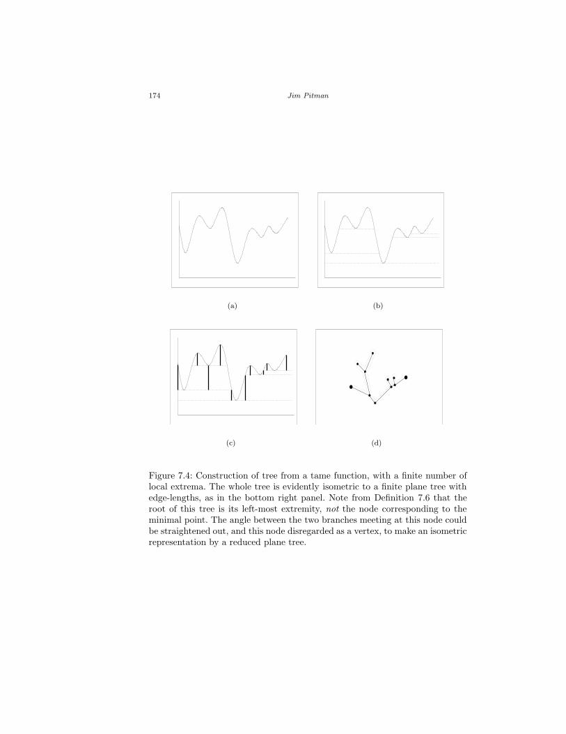
174 Jim Pitman

(a) (b)

(c) (d)

Figure 7.4: Construction of tree from a tame function, with a finite number oflocal extrema. The whole tree is evidently isometric to a finite plane tree withedge-lengths, as in the bottom right panel. Note from Definition 7.6 that theroot of this tree is its left-most extremity, not the node corresponding to theminimal point. The angle between the two branches meeting at this node couldbe straightened out, and this node disregarded as a vertex, to make an isometricrepresentation by a reduced plane tree.

7.9. FURTHER DEVELOPMENTS 175

T1 T2 T3 T1DT1

G

0

(a) (b)

Figure 7.5: subtree(2B; GT1 , T1, . . . , TN), as in Lemma 7.10

176 Jim Pitman

o

oo

o

o

oo

o

o

o

o

o

root 1

32

4

5

9 10

76

8

11

12

s t s t s t s t s t s t1 1 2 2 3 3 4 4 5 5 6 6

Figure 7.6: A forest subtree(B; 0, t1, t2, . . . , t6) and its Harris path. Notesi = arg minti−1≤s≤ti

B(s). Vertices of the forest are labeled in alternating order,so vertex 2n corresponds to time tn and vertex 2n− 1 to time sn.

7.9. FURTHER DEVELOPMENTS 177

(a)

(b)

(c)

Figure 7.7: Forest growth by wrapping one forest around another

178 Jim Pitman

Chapter 8

Brownian local times,

branching and Bessel

processes

It is well known that the random occupation measure induced by the samplepath of a Brownian motion B = (Bt, t ≥ 0) admits a jointly continuous localtime process (Lx

t (B);x ∈ R, t ≥ 0) such that∫ t

0

f(Bs)ds =

∫ ∞

−∞Lx

t (B)f(x)dx.

See [304, 255, 384]. This chapter reviews the basic descriptions of Brownianlocal times in terms of Bessel processes, due to Ray [381] and Knight [254],and interprets these results in terms of random trees and forests embedded inBrownian paths. Then various developments of these descriptions are discussed.

8.1. Stopping at first hitting times Here the Ray-Knight description ofthe process (Lx

T (B);x ∈ R) is recalled for T the first hitting time of a levelby either B or by (L0

t (B), t ≥ 0).8.2. Squares of Bessel processes These are involved in the Ray-Knight

theorems and their variants.8.3. Stopping at fixed times By suitable conditioning, the Ray-Knight the-

ory provides access to the law of (Lxt (B), x ∈ R) for fixed times t.

8.4. Time-changed local time processes Making a change of variable inthe space-parameter of these local time processes for fixed time t, so thatthe quadratic variation in x becomes a new time parameter, leads toJeulin’s identity relating Brownian excursion and its local time process.

8.5. Branching process approximations This section offers some furtherdescriptions of local time processes in terms of branching process approx-imations to squared Bessel processes and their bridges.

8.1. STOPPING AT AN INVERSE LOCAL TIME 179

8.1. Stopping at an inverse local time

Throughout this section let R denote a reflecting Brownian motion on [0,∞),which according to Levy’s theorem [384] may be constructed from a standardBrownian motion either as R = |B|, or as R = B−B, where Bt := inf0≤s≤tBs.Note that if R = |B| then for v ≥ 0

Lvt (R) = Lv

t (B) + L−vt (B) (8.1)

and in particular L0t (R) = 2L0

t (B). For ` ≥ 0 let

τ` := inft : L0t (R) > ` = inft : L0

t (B) > `/2. (8.2)

For 0 ≤ v < w let

D(v, w, t) := number of downcrossings of [v, w] by R before t

From the structure of the Brownian forest described in Section 7.6 there is thefollowing basic description of the process counting downcrossings of intervals upto an inverse local time. See also [426] for more about Brownian downcrossingsand their relation to the Ray-Knight theorems.

Corollary 8.1. [323] The process

(D(v, v + ε, τ`), v ≥ 0)

is a time-homogeneous Markovian birth and death process on 0, 1, 2 . . ., withstate 0 absorbing, transition rates

n− 1nε←− n

nε−→ n+ 1

for n = 1, 2, . . ., and initial state D(0, ε, τ`) which has Poisson(`/(2ε)) distribu-tion.

Proof. According to Theorem 7.15 , applied to R := B − B run until B firstreaches −`/2, the number D(v, v+ ε, τ`) is the number of branches at level v ina critical binary (0, ε) branching process started with a Poisson(`/(2ε)) numberof initial individuals, so the conclusion is immediate.

From the Poisson distribution of D(0, ε, τ`), and the law of large numbers,

limε↓0

εD(0, ε, τ`) = ` almost surely

and similarly, for each v > 0 and ` > 0, by consideration of excursions of Raway from level v

limε↓0

2εD(v, v + ε, τ`) = Lvτ`

(R) almost surely.

180 Jim Pitman

According to Corollary 8.1, this process (2εD(v, v + ε, τ`), v ≥ 0), which servesas an approximation to (Lv

τ`(R), v ≥ 0), is a Markov chain whose state space is

the set of integer multiples of 2ε, with transition rates

x− 2εx

2ε2←− xx

2ε2−→ x+ 2ε

for x = 2εn > 0. The generatorGε of this Markov chain acts on smooth functionsf on (0,∞) according to

(Gεf)(x) =x

2ε2f(x− 2ε) +

x

2ε2f(x+ 2ε)− x

ε2f(x)

= 4x1

(2ε)2[

12f(x− 2ε) + 1

2f(x+ 2ε)− f(x)]

→ 4x1

2

d2

dx2f as ε→ 0.

Hence, appealing to almost any result on approximation of diffusions by Markovchains [265, 264], we obtain:

Theorem 8.2. (Ray [381], Knight [254]) For each fixed ` > 0, and τ` := inft :L0

t (R) > `, where R = |B|,

(Lvτ`

(R), v ≥ 0)d= (Q

(0)`,v , v ≥ 0) (8.3)

where the process on the right hand side is the Feller diffusion on [0,∞) withabsorbtion at 0, and generator

4x1

2

d2

dx2(8.4)

acting on smooth functions vanishing in a neighbourhood of 0.

Exercises

8.1.1. (Ray-Knight) Let T` := τ2` := inft > 0 : L0t (B) = `. Then the pro-

cesses (LvT`

(B), v ≥ 0) and (L−vT`

(B), v ≥ 0) are two independent copies of

(Q(0)`,v , v ≥ 0).

Notes and comments

Many proofs and extensions of the basic Ray-Knight theorems can be found inthe literature. See for instance [233, 384, 348, 426, 219] and papers cited there.

8.2. SQUARES OF BESSEL PROCESSES 181

8.2. Squares of Bessel processes

The Feller diffusion appearing on the right side of (8.3) is the particular case

δ = 0 of a squared Bessel with parameter δ started at ` ≥ 0, denoted (Q(δ)`,v , v ≥

0). This Markov process with state space [0,∞) can be defined [384, Ch. XI]for each δ ≥ 0 as the unique non-negative strong solution of the Ito stochasticdifferential equation (SDE)

Q0 = `; dQv = δ dv + 2√

Qv dβv (8.5)

where (βv, v ≥ 0) is a BM. For δ < 0, such a process can be uniquely definedup to its hitting time of 0 as the solution of this SDE, with either killing or

absorbtion at 0. Denote the law of (Q(δ)`,v , v ≥ 0) by BESQ

(δ)` , and denote

by BESQ(δ) the Markov process with state space [0,∞) determined by this

collection of laws (BESQ(δ)` , ` ≥ 0). For an account of the basic properties of

these processes see [384]. The parameter δ, which simply represents a constantdrift coefficient, is often called the dimension of the squared Bessel process, dueto the following well known consequence of Ito’s formula: that if (Bi,v , v ≥ 0)for i = 1, 2, . . . is a sequence of independent standard Brownian motions, then

(Q(δ)`,v , v ≥ 0)

d=

(

(√`+B1,v)2 +

δ∑

i=2

B2i,v , v ≥ 0

)

(δ = 1, 2, . . .). (8.6)

The squared Bessel processes and their bridges, especially for δ = 0, 2, 4, areinvolved in the description of the local time processes of numerous Brownianpath fragments [254, 381, 436, 365]. For instance, if H1(X) := inft : Xt = 1,then according to Ray and Knight

(LvH1(B)(B), 0 ≤ v ≤ 1)

d= (Q

(2)0,1−v, 0 ≤ v ≤ 1). (8.7)

The appearance of BESQ(δ) processes embedded in the local times of Brown-ian motion is best understood in terms of the construction of these processesas weak limits of Galton-Watson branching processes with immigration, andtheir consequent interpretation as continuous state branching processes withimmigration [233].

For instance, there is the following expression of the Levy-Ito representa-tion of squared Bessel processes, and its interpretation in terms of Brownianexcursions [365], which are recalled in Exercise 8.2.4 .

Theorem 8.3. Le Gall-Yor [278] For R a reflecting Brownian motion on [0,∞),with R0 = 0, let

Y(δ)t := Rt + L0

t (R)/δ (t ≥ 0).

Then for δ > 0 the process of ultimate local times of Y (δ) is a copy of BESQ(δ)0 :

(Lv∞(Y (δ)), v ≥ 0)

d= (Q

(δ)0,v , v ≥ 0). (8.8)

182 Jim Pitman

This has an immediate interpretation in terms of Brownian trees [2]. If R isconstructed as R = B −B, so L0

t (R) = −2B(t), then

tree(B) = tree(B − 2B) = tree(Y (2))

where Y (2) is a copy of the three-dimensional Bessel process R3. Thus Lv∞(Y (2))

is the mass density of vertices in either tree(B) or tree(Y (2)) at distance vfrom the root 0, where mass refers to Lebesgue measure on R≥0. That thisprocess should be regarded as a continuous state branching process with immi-gration is intuitively obvious from the Poisson structure of the forest of subtreesof tree(B) attached to its infinite branch Proposition 7.8 . Similarly Lv

∞(Y (δ))is the mass density of vertices in tree(Y (δ)) at distance v from the root 0. Byconstruction of Y (δ), its tree is derived from tree(Y (2)) by simply stretchingdistances along the infinite branch of tree(Y (2)) by a factor of 2/δ, and leavingthe same Poisson forest of subtrees attached to this branch. Thus δ is simplya parameter governing the rate of appearance of Brownian subtrees of varioussizes along the infinite branch of Y (δ), that is to say a rate of immigration, orrate of generation of new Brownian subtrees, in a continous state branchingprocess.

Exercises

8.2.1. (Knight) Use the well known construction of a copy of R from B, bydeletion of all negative excursions of B, to show that the process (Lv

H1(R)(R), 0 ≤v ≤ 1) has the same distribution as the processes displayed in (8.7). See alsoKnight [255], McKean [304].

8.2.2. (Williams [436]) Deduce (8.7) from (8.8) for δ = 2, and vice-versa, usingWilliams’ time reversal identity [384] relating the path of B on [0, H1(B)] tothat of R3 on [0,K1], where K1 is the last time that R3 hits 1.

8.2.3. [384] Deduce from the SDE definition of BESQ(δ)` the additivity property

[401] that for all non-negative δ, δ′, ` and `′ the sum of a BESQ(δ)` process and

an independent BESQ(δ′)`′ process is a BESQ

(δ+δ′)`+`′ process. For positive integer

δ, δ′ this is obvious from (8.6). Show that the law of BESQ(δ)` for all δ ≥ 0 and

` ≥ 0 is uniquely determined by the additivity property and the prescription(8.6) for δ = 1.

8.2.4. [365] As a consequence of the additivity property, the family of BESQ(δ)`

processes can be constructed on a common probability space in such a way

that the path-valued process (Q(δ)`,v , v ≥ 0)δ≥0,`≥0 is increasing with stationary

independent increments. The C[0,∞)-valued processes

(Q(δ)0,v, v ≥ 0)δ≥0 and (Q

(0)`,v , v ≥ 0)`≥0 (8.9)

are then two independent increasing processes with stationary independent in-crements, the jumps of which are two independent Poisson processes of points

8.3. STOPPING AT FIXED TIMES 183

in C[0,∞) governed by two σ-finite Levy measures M and N , which may bedescribed as follows: M is the distribution of the ultimate local time process(L∞,v(X), v ≥ 0) for the co-ordinate process X on C[0,∞) subject to Ito’sσ-finite law ν of Brownian excursions, and N =

∫∞0Mudu where Mu is the

measure on C[0,∞) under which X [0, u] ≡ 0 and X [u,∞) has distribution M .Under M the co-ordinate process X is Markovian with the BESQ(0) semigroup,with almost every path starting at 0.

8.2.5. [278] (Proof of Theorem 8.3) Deduce (8.8) for general δ > 0 from its

special case δ = 2, using the additivity property of BESQ(δ)0 .

Notes and comments

See Le Gall [274] for developments of these ideas in the context of Markoviansuper-processes. See [365, 348, 384] for descriptions of the infinitely divisible

distribution of∫∞0Q

(δ)`,vµ(dv), for suitable measures µ, in terms of the solutions

of Sturm-Liouville equations associated with µ, and treatment of the same prob-lem for squared Bessel bridges. Carmona-Petit-Yor [86] found a construction of

BESQ(δ)x for δ < 0 < x which is similar to (8.8) See also [340, 343].

8.3. Stopping at fixed times

Features of the distribution of the Brownian local time process (Lxt (B), x ∈ R),

for a fixed time t, are of interest in a number of contexts. In principle, the familyof distributions of these local time processes is determined by the Ray-Knightdescription of the joint law of (Lx

T (B), x ∈ R) and BT for T an exponential timeindependent of B, as considered in [63]. In practice, it is hard work to invertthe implicit Laplace transform to gain anything explicit from this description,though this can certainly be done, as shown by Leuridan [283]. A simpler wayto access the structure of the process (Lx

t (B), x ∈ R) for fixed t is to exploitthe branching process approximation to do computations in a combinatorial set-ting without technical complication, then appeal to some general approximationtechnique to justify passage to the Brownian limit.

The effectiveness of this approach is well illustrated by the following prob-lem, which arises naturally from the asymptotics of random forests and ran-dom mappings. Let Bbr

` denote a standard Brownian bridge Bbr conditioned onL0

1(Bbr) = `. The problem is to describe the law of the process (Lv1(|Bbr

`/2|), v ≥0) as explicitly as possible. Note that the conditioning on L0

1(Bbr) = `/2 makesthe process (Lv

1(|Bbr`/2|), v ≥ 0) start at L0

1(|Bbr`/2|) = `. The structure of excur-

sions of |Bbr`/2| away from 0 can be described as follows: the excursion intervals

of |Bbr`/2| define an exchangeable interval partition of [0, 1], whose law is defined

by conditioning the ( 12 ,

12 ) partition generated by Bbr to have 1

2 -diversity equal

to `/√

2. By the switching identity (4.71) and the Ray-Knight description (8.3),

184 Jim Pitman

for each ` > 0

(Lv1(|Bbr

`/2|), v ≥ 0)d=

(

Q(0)`,v , v ≥ 0

∣∣∣∣

∫ ∞

0

Q(0)`,vdv = 1

)

(8.10)

Note that for ` = 0 the left side of (8.10) has direct meaning as the local timeprocess of Bex, but the right hand side does not because 0 is an absorbing statefor BESQ(0). We will return to this point after stating the following theorem.

Theorem 8.4. [358] For each t > 0 and ` ≥ 0, a process Q = (Q`,t,v, v ≥ 0)with continuous paths such that

(Lv1(|Bbr

`/2|), v ≥ 0)d= (Q`,1,v, v ≥ 0), (8.11)

can be defined as the unique strong solution of the Ito SDE

Q0 = `; dQv = δv(Q)dv + 2√

Qvdβv (8.12)

where β is a Brownian motion and

δv(Q) := 4−Q2v

(t−∫ v

0 Qudu)−1

(8.13)

with the convention that the equation for Q is to be solved only on [0, Vt(Q))and that Qv = 0 for v ≥ Vt(Q) where

Vt(Q) := infv :∫ v

0Qudu = t. (8.14)

Note that for each ` ≥ 0 and t > 0 the random time Vt(Q) is strictly positiveand finite a.s., and the left limit of Q at time Vt(Q) exists and equals 0 a.s..A proof of this theorem will be sketched in Section 8.5 , based on a branchingprocess approximation.

It is easily seen by Brownian scaling how to interpret the process (Q`,t,v, v ≥0) for all t > 0 and ` ≥ 0: if Bbr,t denotes a Brownian bridge from 0 to 0 oflength t, then

(Lvt (|Bbr,t|), v ≥ 0 |L0

t (|Bbr,t|) = `)d= (Q`,t,v, v ≥ 0). (8.15)

Provided ` > 0 this process may also be interpreted as a BESQ(0)` process

(Q(0)`,v , v ≥ 0) conditioned on

∫∞0 Q

(0)`,vdv = t. Call (8.15) the local time inter-

pretation of Q. The SDE (8.12) defining Q in (8.15) is a generalization of theBESQ(δ) SDE (8.5) in which the drift δv at level v is a path dependent functionof the unknown process Q, namely δv := 4 − Q2

v(t −∫ v

0 Qudu)−1, which maybe of either sign. It is well known that for fixed δ < 0 and any initial value` > 0 the BESQ(δ) SDE has a pathwise unique solution on a stochastic interval[0, V0) such that the solution approaches 0 at time V0. The BESQ(δ) process forδ ≤ 0 is known [365] to arise as a Doob h-process by conditioning a BESQ(4−δ)

process to hit 0. To get some feeling for the effect of the path dependent drift

8.3. STOPPING AT FIXED TIMES 185

δv, keep in mind that the local times process (Lvt (|Bbr,t|), v ≥ 0) is subject to

the constraint ∫ ∞

0

Lut (|Bbr,t|)du = t

so the random variable

t−∫ v

0

Lut (|Bbr,t|)du =

∫ ∞

v

Lut (|Bbr,t|)du,

representing the time spent by |Bbr,t| above v, is determined as a function ofthe local times of |Bbr,t| at levels below v. According to the theorem, giventhe local times at all levels below v, the local time process evolves over thenext infinitesimal level increment like a squared Bessel process of dimensionδv := 4− βv , where βv is the square of the local time at level v relative to thetime above v. Note that if the local time at level v is close to zero, but the timeabove v is not, then β is close to zero, so the local time process is forced away

from 0 in much the same way as a BESQ(4)0 escapes from 0. For ` > 0 it is

known [384] that the BESQ(δ)` process hits zero in finite time only if δ < 2.

So the expression δv = 4− βv implies that the local time process cannot reachzero before a level v such that βv > 2, meaning the square of the local time atv exceeds twice the time above v. Much sharper results could be given in thesame vein.

As remarked below (8.10), this formula has no direct meaning for ` = 0,and t > 0, even though the process (Q0,t,v, v ≥ 0) is a well defined processidentical in law to the process of local times of Bex,t, a Brownian excursion oflength t. However, formula (8.10) amounts to the following identity of probabilitymeasures on C[0,∞):

BESQ(0)` =

∫ ∞

0

BESQ(0)`,t P(τ` ∈ dt) (` > 0) (8.16)

where BESQ(0)` denotes the law of C[0,∞) of a BESQ

(0)` process (Q

(0)`,v , v ≥ 0),

τ` :=

∫ ∞

0

Q(0)`,vdv

d= (`/2)2/B2

1

and BESQ(0)`,t is the law of (Q

(0)`,v , v ≥ 0) given τ` = t. Here we exploit the

Ray-Knight theorem (8.3) to suppose for convenience that the entire family

of BESQ(0)` processes (Q

(0)`,v , v ≥ 0) is defined on the same probability space

(Ω,F ,P) as a basic Brownian motion B, according to the formulaQ(0)`,v := Lv

τ`(R)

where R = |B| and (τ`, ` ≥ 0) is the inverse local time process of R at 0, as in(8.2). If this form (8.16) of formula (8.10) is divided by `, and the limit taken as` ↓ 0, the result is the following formula for the Levy measureM of the increasingpath valued process with stationary independent increments (Q`,t,v, v ≥ 0)`≥0,as further interpreted in Exercise 8.2.4 :

M =

∫ ∞

0

BESQ(0)0,t

t−3/2dt√2π

(8.17)

186 Jim Pitman

where BESQ(0)0,t is the law on C[0,∞) of

(Q0,t,v, v ≥ 0)d= (Lv

t (Bex,t), v ≥ 0).

Thus M is in many respects like a law of excursions of BESQ(0) away from 0.But it is not possible to concatenate such excursions to form a process, becauseif µ denotes the M distribution of H0, the return time to 0, then µ fails to satisfythe necessary condition

∫∞0

(1 − e−x)µ(dx) < ∞ for µ to be the Levy measureof an inverse local time process.

Notes and comments

This section is based on [358].

8.4. Time-changed local time processes

Keep in mind that the “time” parameter of the local time process (Q`,t,v, v ≥ 0)is actually a level v, so perhaps we should speak instead of “space-changed”local time processes. Consider some reformulations of Theorem 8.4 which canbe made by stochastic calculus. For a non-negative process Y := (Ys, 0 ≤ s ≤ 1)admitting a continuous occupation density process (Lv

1(Y ), v ≥ 0), define a

process L(Y ) := (Lu(Y ), 0 ≤ u ≤ 1) by Lu(Y ) := Lv(u)1 (Y ) where v(u) :=

supy ≥ 0 :∫∞

y Lx1dx > u. So Lu(Y ) is the local time of Y at a level v(u)

above which Y spends time u. This definition is suggested by the remarkableresults of Jeulin [220, p. 264] that

L(Bex)d= 2Bex (8.18)

and Biane-Yor [61, Th. (5.3)] that

L(|Bbr|) d= 2Bme (8.19)

where Bex and Bme are standard Brownian bridge and meander, respectively.If we recall that Bme conditioned on Bme(1) = r is a BES(3) bridge from 0 tor, say R0→r

3 , then (8.19) implies

L(|Bbr`/2|)

d= 2R

0→`/23 . (8.20)

Conversely, (8.19) is recovered from (8.20) and the fact that L01(Bbr)

d= Bme(1).

Moreover, (8.18) is the special case ` = 0 of (8.20). Now either of the descriptions(8.20) and (8.11) can be derived from the other, using the fact that Rx→y

3 is thetime reversal of Ry→x

3 , the description of these bridges as solutions of an SDE,and the computation of Lemma 8.5 below, which transforms the SDE solved by(Lv

1(|Bbr`/2|), v ≥ 0) into that solved by (Lu(|Bbr

`/2|), 0 ≤ u ≤ 1).The transformation between the two SDEs is done by the following Lemma.

This corrects [358, Lemma 14], where the process R should obviously be startedat `/2 instead of `.

8.4. TIME-CHANGED LOCAL TIME PROCESSES 187

Lemma 8.5. For ` ≥ 0, t > 0 let R` be the process derived from (Q`,1,v, v ≥ 0)via the formula

2R`s := Q`,t,v for the least v :

∫ v

0

Q`,1,udu = s, where 0 ≤ s ≤ 1 (8.21)

Then R` d= R

`/2→03 and (Q`,1,v, v ≥ 0) can be recovered from R` via the formula

Q`,1,v = 2R`s for the least s :

∫ s

0

dr

2R`r

= v. (8.22)

Consequently, if R` d= R

`/2→03 , then Q defined by (8.22) has the same distribu-

tion as Q defined by the SDE (8.12).

Proof. Starting from three independent standard Brownian bridges Bbri , i =

1, 2, 3, for x, y ≥ 0 let

Rx→y3 (u) :=

√

(x+ (y − x)u+Bbr1,u)2 + (Bbr

2,u)2 + (Bbr3,u)2 (0 ≤ u ≤ 1).

(8.23)Ito’s formula implies that the process Rx→y

3 can be characterized for each x, y ≥0 as the solution over [0, 1] of the Ito SDE

R0 = x; dRs =

(1

Rs+

(y −Rs)

(1− s)

)

ds + dγs (8.24)

for a Brownian motion γ. The recipe (8.22) for inverting the time change (8.21)is easily checked, so it suffices to show that if R := (R`

s, 0 ≤ s ≤ 1) solvesthe SDE (8.24), for (x, y) = (`/2, 0) and some Brownian motion γ, then Q :=(Q`,1,v, v ≥ 0) defined by (8.22) solves the SDE (8.12) for some Brownian motionβ. But from (8.21) and (8.22)

dQv = 2 dRs where s =

∫ v

0

Qudu

A level increment dv for Q corresponds to a time increment ds = Qvdv for R,and Rs = Qv/2, so

dQv = 2

(

1

Qv/2− Qv/2

(1−∫ v

0 Qudu)

)

Qvdv + 2√

Qvdβv (8.25)

for some other Brownian motion β, where the factor√Qv appears in the diffu-

sion term due to Brownian scaling, and the equation (8.25) simplifies to (8.12).

As a technical point, the definition of β above the level∫ t

0dr/2R`,0,t

r when Qhits 0 may require enlargement of the probability space. See [384, Ch. V] for arigorous discussion of such issues.

188 Jim Pitman

Exercises

8.4.1. Show that

supv≥0

Lv1(|Bbr|) d

= 2 sup0≤u≤1

Bmeu

d= 4 sup

0≤u≤1|Bbr

u | (8.26)

where Bme is a Brownian meander of length 1, the second equality is due toKennedy [238], and the distribution of sup0≤u≤1 |Bbr

u | is given by the well knownKolmogorov-Smirnov formula. Also

(L01(|Bbr|), sup

v≥0Lv

1(|Bbr|)) d= 2(Bme

1 , sup0≤u≤1

Bmeu ) (8.27)

the joint density of which can be read from known results for the Brownianmeander [209].

8.4.2. [358, Corollary 18] Conditionally given

L01(Bbr) = ` and

∫ 1

0

1(Bbru > 0)du = a,

the processes (Lv1(Bbr), v ≥ 0) and (L−v

1 , v ≥ 0) are independent copies of(Q`,a,v, v ≥ 0) and (Q`,1−a,v, v ≥ 0) respectively.

Notes and comments

This section is based on [358]. Perkins [338] showed that for each fixed t > 0the process of local times of B at levels v up to time t is a semi-martingale as vranges over all real values, and he gave the semi-martingale decomposition of thisprocess. Jeulin [220] gave a version of Perkins results that allows conditioning onBt. See [167] and [168] for more information regarding the distribution of localtimes of Bex and |Bbr|. Knight [258, 259] treats the related problem of describing

the distribution of∫ 1

0 |Bbr` (u)|du. See also [342]. Norris-Rogers-Williams [326,

Th. 2]showed that the distribution of a local time process derived from anotherkind of perturbed Brownian motion, with a drift depending on its local timeprocess, can be characterized by a variation of the Bessel square SDE like (8.12),but with a different form of path dependent drift coefficient δv(Q). See also[438] and papers cited there for various other Ray-Knight type descriptions ofBrownian local time processes, and further references on this topic.

8.5. Branching process approximations

The following result in the theory of branching processes, first indicated byFeller [149] and further developed by Lamperti [269, 268] and Lindvall [285],

generalizes the approximation of (Q(0)`,v , v ≥ 0) by a continuous time branching

8.5. BRANCHING PROCESS APPROXIMATIONS 189

process which was made in the previous section. See also [386]. Let Zk(h) forh = 0, 1, 2, . . . be the number of individuals in generation h of a Galton-Watsonprocess started with k individuals in which the offspring distribution has mean1 and finite variance σ2 > 0, and let Zk(h) be defined for all h ≥ 0 by linearinterpolation between integers. Then as both m→∞ and k →∞

(2

σmZk(2mv/σ), v ≥ 0

)

d→ (Q(0)`,v , v ≥ 0) if

2k

σm→ `, (8.28)

where the limit is BESQ(0)` . To check the normalizations in (8.28), observe

that if the process on the left side has value x at v such that 2mv/σ equals aninteger h, then Zk(h) = xσm/2. The number Zk(h+1) in the next generation ofthe branching process therefore has variance (xσm/2)σ2. The increment of theprocess on the left side over the next v-increment of σ/(2m) has this variancemultiplied by (2/σm)2. So along the grid of multiples of σ/(2m), the varianceof increments of the normalized process on the left side per unit v-increment,from one grid point to the next, given the normalized process has value x at thefirst grid point, is

(xσm

2

)

σ2

(2

σm

)2 ( σ

2m

)−1

= 4x = (2√x)2

in accordance with the BESQ(0) SDE. Let (Zk,n(h), h ≥ 0) defined by condi-tioning (Zk(h), h ≥ 0) on the event that its total progeny

∑∞h=0 Zk(h) equals n,

so by definition

(Zk,n(h), h ≥ 0)d= (Zk(h), h ≥ 0 |∑∞

h=0 Zk(h) = n) (8.29)

where it is assumed now that the offspring distribution is aperiodic, so theconditioning event has strictly positive probability for all sufficiently large n.Then it is to be anticipated from (8.28) and (8.29) that as n→∞(

2

σ√nZk,n(2

√nv/σ), v ≥ 0

)

d→ (Q`,1,v, v ≥ 0) provided2k

σ√n→ ` (8.30)

for some ` ≥ 0 where (Q`,1,v, v ≥ 0) may be identified by conditioning the limit

BESQ(0)` process in (8.28) on its integral being equal to 1, as implied by (8.10),

and the definition is extended to ` = 0 by weak continuity. This intuitivelyobvious identification of the limit can be justified by regularity of the solutionof the basic SDE (8.12) as a function of its parameters, provided it is shown thatthe weak convergence (8.30) holds with the limit defined as the pathwise uniquesolution of the SDE (8.12). So let us now see how to derive the basic SDE (8.12)directly from combinatorial considerations. Note that if Zk,n(h) is interpretedas the number of vertices at level h in a forest with n vertices defined by acollection of k family trees, one for each initial individual in the Galton-Watsonprocess, then for h = 0, 1, . . . the random variable

Ak,n(h) := n−h∑

i=0

Zk,n(h) (8.31)

190 Jim Pitman

represents the number of vertices in the forest strictly above level h.

Lemma 8.6. Fix 1 ≤ k < n. A sequence (Z(h), h = 0, 1 . . .) has the samedistribution as a Galton-Watson process with a Poisson offspring distributionstarted with k individuals and conditioned on its total progeny being equal to n,if and only if the sequence evolves by the following mechanism: Z(0) = k andfor each h = 0, 1 . . .

(Z(h+1) |Z(i), 0 ≤ i < h, Z(h) = z, A(h) = a)d= 1+binomial(a−1, z/(a+z)),

(8.32)

where A(h) := n −∑hi=0 Z(i) and binomial(m, p) is a binomial(m, p) random

variable, with the conventions binomial(−1, p) = −1 and binomial(0, p) = 0.

See the exercises for a proof and variations of this lemma. Granted the lemma,consider the rescaled process on the left side of (8.30) in the Poisson case,so σ = 1, in an asymptotic regime with n → ∞ and 2k/

√n → ` for some

` ≥ 0. Let Wk,n(h) := (Zk,n(h), Ak,n(h)). From (8.32), in the limit as n, zand a tend to ∞ with 2z/

√n → x and a/n → p, for integer h the increment

∆k,n(h) := Zk,n(h + 1) − Zk,n(h) is such that the corresponding normalizedincrement ∆∗

k,n(h) := 2∆k,n(h)/√n has the following conditional mean and

variance given a history (Zk,n(i), 0 ≤ i ≤ h) with Wk,n(h) = (z, a):

E(∆∗k,n(h) |Wk,n(h) = (z, a)) =

2√n

(

1 +(a− 1)z

a+ z− z)

≈(

4− x2

p

)1

2√n

V ar(∆∗k,n(h) |Wk,n(h) = (z, a)) =

4

n

(a− 1)za

(a+ z)2≈ 4x

1

2√n

where the relative errors of approximation are negligible as n → ∞, uniformlyin h, provided x < 1/ε and p > ε which can be arranged by a localizationargument, stopping the normalized process when either its value exceeds x orits integral exceeds 1 − p. Since ∆∗

k,n(h) is the increment of the normalized

process over a time interval of length 1/(2√n), and the value of p ≈ Ak,n(h)/n

can be recovered from the path of the normalized process with a negligible errorvia

p ≈ Ak,n(h)

n= 1− 1

n

h∑

i=0

Zk,n(h) ≈ 1−∫ h/(2

√n)

0

2√nZk,n(2

√nv) (8.33)

these calculations show that the normalized process is governed asymptoticallyby the SDE (8.12)-(8.13) presented in Theorem (8.4). It can be shown by stan-dard arguments [384] that the SDE has a unique strong solution. So the pre-ceding argument, combined with known results regarding the approximation ofa Markov chain by the solution of an SDE [265] [264, Theorem 5.4], shows thatthe weak limit of the normalized and conditioned branching process solves theSDE (8.12)-(8.13).

8.5. BRANCHING PROCESS APPROXIMATIONS 191

Exercises

8.5.1. (Proof of Lemma 8.6) [358, Lemma 8] Let X1, X2, . . . be a sequenceof independent random variables with some distribution p on 0, 1, 2, . . ., andset Sj = X1 + · · · + Xj . Fix 1 ≤ k < n with P (Sn = n − k) > 0. Let(Zk,n(h), h = 0, 1, 2, . . .) be a Galton-Watson branching process with offspringdistribution p started with k individuals and conditioned to have total progenyn, and define Ak,n(h) by (8.31), and set Wk,n(h) := (Zk,n(h), Ak,n(h)). Showthat Wk,n(h), h = 0, 1, 2, . . . is a Markov chain, with initial state (k, n− k), andthe following transition probabilities which do not depend on n and k: givenWk,n(h) = (z, a) the distribution of Zk,n(h+1) is obtained by size-biasing of thedistribution of Sz given Sz+a = a, and Ak,n(h+1) = a−Zk,n(h+1). In particular,for a Poisson distribution the law of Sz given Sz+a = a is binomial(a, z/(z+a)).A size-biased binomial(n, p) variable is 1 plus a binomial(n− 1, p) variable, andLemma 8.6 follows.

8.5.2. (Combinatorial interpretation of Lemma 8.6) Fix k and n with1 ≤ k ≤ n and for h = 0, 1, . . . let Lh := Lh(Fk,n) be the number of vertices atlevel h of Fk,n, a uniformly distributed random forest of k rooted trees labeled by[n]. Then L0 = k and the distribution of the sequence L1, L2, . . . is determinedbe the following prescription of conditional laws: for each h = 0, 1, . . .

dist(Lh+1 |L0, . . . , Lh) = dist(1 + binomial(Ah − 1, Lh/(Ah + Lh) (8.34)

where Ah := n−∑hi=0 Li and binomial(n, u) denotes a binomial random variable

with parameters n and u ∈ (0, 1).

8.5.3. (Further combinatorial interpretation of Lemma 8.6) The pre-vious exercise shows that for each (k, n) the bivariate sequence ((Lh, Ah), h =0, 1, . . .) has the Markov property. The transition probabilities are inhomoge-neous, but they have a recursive property, reflecting the fact that for any givenh the random variable Ah represents the number of vertices of the forest strictlyabove level h, while Ah + Lh is the number of vertices at or above level h. Thesimplifying feature of a uniform forest that given the forest at levels up to andincluding h leaves room for Ah vertices above h, the number Lh+1 of these ver-tices at level h + 1 are selected as the children of Lh roots in a uniform forestof Lh trees with given roots in a set of size Lh +Ah. This basic recursive prop-erty, which can be seen by a direct combinatorial argument, can be expressedas follows. Let Ln,h denote the number of vertices at level h of a random forestwhich given Ln,0 = k is uniformly distributed on all forests of k trees labeled

by [n], and set An,h := n−∑hi=0 Ln,i Then for each h ≥ 0 and j ≥ 0

(Ln,h+j , j ≥ 0 |Ln,i, 0 ≤ i ≤ h with Ln,h = m,An,h = a)

has the same distribution as

(La+m,j , j ≥ 0 |La+m,0 = m).

8.5.4. [358] What is the Brownian analog of the property of uniform randomforests described in the previous exercise?

8.5.5. (Problem) Does (8.30) require any further conditions on the offspringdistribution of the critical branching process besides finite non-zero variance?

Notes and comments

The basic Ray-Knight theorems for Brownian local times have been extendedfrom Brownian motion to real-valued diffusions, using Feller’s representation ofsuch diffusions by space and time changes of Brownian motion. These resultswere extended in [131, 298] to a large class of Markov processes admitting localtimes. But for these extensions to discontinuous Markov processes, the Markovproperty of local times in the space variable is lost. See also [282, 348, 130]regarding local times of processes indexed by circles, trees, and graphs.

The properties of the local time processes of Brownian excursion and reflect-ing Brownian bridge discussed here are closely related to the interval fragmen-tation process (Yv, v ≥ 0) derived from one of the processes X = Bex, |Bbr| or|Bbr

` | by letting Yv be the collection of ranked lengths of the random open sett : Xt > v. It is clear from the present discussion that each of these processes(Yv , v ≥ 0) is Markovian, with the same transition mechanism, whereby differ-ent interval lengths are fragmented independently according to rescaled copiesof the interval fragmentation induced by a single excursion Bex. This processis a basic example of the general class of self-similar fragmentations studied byBertoin [46], which illustrates the phenomenon of “erosion” or loss of mass inthe fragmentation process, since the total mass of the process after time v is

∫ 1

0

1(Xt > v) dt =

∫ ∞

v

Lx1(X) dx.

Thus the local time Lv1(X), which is a measurable function of the sequence of

ranked lengths Yv, is the rate of erosion of mass at time v in the fragmentationprocess, and the SDE (8.12) may be interpreted as describing the dynamics oferosion in the fragmentation process. One can also think of Lv

1(X) as the densityof mass at level v in a forest of Brownian trees of mass

∫∞vLx

1(X)dx. As thelevel v rises, the fragmentation process describes how trees rooted on a valleyfloor disappear beneath a rising tide as the valley is flooded.

192

8.5. BRANCHING PROCESS APPROXIMATIONS 193

194 Jim Pitman

Chapter 9

Brownian bridge

asymptotics for random

mappings

This chapter reviews Brownian bridge asymptotics for random mappings, firstdescribed in 1994 by Aldous and Pitman. The limit distributions as n→∞, ofvarious functionals of a uniformly distributed random mapping from an n ele-ment set to itself, are those of corresponding functionals of a Brownian bridge.Similar results known to hold for various non-uniform models of random map-pings, according to a kind of invariance principle. A mapping Mn : [n] → [n]can be identified with its digraph i→Mn(i), i ∈ [n], as in Figure 1.

Note how the mapping digraph encodes various features of iterates of themapping. A mapping digraph can be decomposed as a collection of rooted treestogether with some extra structure (cycles, basins of attraction). If each rootedtree is regarded as a plane tree and encoded by its Harris walk, defined by depth-first search following Harris [193], then given some ordering of tree-components,one can concatenate these Harris walks to define a mapping-walk which encodesnumerous features of Mn.

From now on, we shall be interested in a uniformly distributed random map-ping Mn. The connection between random mappings and Brownian bridge, firstdeveloped in [17], can be summarized as follows.

• For a uniform random mapping, the induced distribution on tree-componentsis such that the tree-walks, suitably normalized, converge to Brownian ex-cursion as the tree size increases to infinity. So it is to be expected thatthe mapping-walks, suitably normalized, should converge to a limit processdefined by some concatenation of Brownian excursions.

• With an appropriate choice of ordering of tree components, the weak limitof normalized mapping walks is reflecting Brownian bridge.

Brownian bridge asymptotics for random mappings 195

49

32

12

43

21

10

36

47

05

11

25

02

39

4550

13

42

46

27

28

31

24

19

01

33

26

48

40

37

18

08

30 09 44

06 03 07 20 17 23

34 41 22 29

04

38 35

16 14 15

Figure 9.1: Digraph of a mapping M50 : [50]→ [50]

The subtle issue is how to order the tree components so that both

a) the mapping-walk encodes structure of cycles and basins of the mapping,and

b) the limit in distribution of the normalized mapping-walk can be explicitlyidentified.

How this can be done is discussed in some detail in the following sections,which are organized as follows:

9.1. Basins and trees deals with the definitions of basins and trees.9.2. Mapping walks introduces two variants of the mapping walk.9.3. Brownian asymptotics contains the main result: the scaled mapping-

walk derived from a uniform random mapping Mn, with 2n steps of size±1/√n per unit time, converges in distribution to 2|Bbr| where Bbr is a

standard Brownian bridge.9.4. The diameter As an application of the main result, the diameter of the

digraph of Mn, normalized by√n, is shown to converge in distribution to

an unusual functional of Bbr.9.5. The height profile The normalized height profile of the forest derived

from Mn converges weakly to the process of local times of |Bbr|.9.6. Non-uniform random mappings This section collects references to

extensions of these asymptotics to various kinds of non-uniform randommappings.

196 Jim Pitman

9.1. Basins and trees

Fix a mapping Mn. It has a set of cyclic points

Cn := i ∈ [n] : Mkn(i) = i for some k ≥ 1,

where Mkn is the kth iterate of Mn. Let Tn,c be the set of vertices of the tree

component of the digraph with root c ∈ Cn. Note that Tn,c might be a trivial treewith just a single root vertex. The tree components are bundled by the disjointcycles Cn,j ⊆ Cn to form the basins of attraction (connected components) of themapping digraph, say

Bn,j :=⋃

c∈Cn,j

Tn,c ⊇ Cn,j with⋃

j

Bn,j = [n] and⋃

j

Cn,j = Cn (9.1)

where all three unions are disjoint unions, and the Bn,j and Cn,j are indexed insome way by j = 1, . . . , |Cn|. Note that each tree component Tn,c is regarded herejust as a subset of [n], which is given the structure of a rooted tree by the actionof Mn. The precise meaning of Bn,j and Cn,j now depends on the conventionfor ordering the cycles, which turns out to be of some importance. Two possibleconventions are the cycles-first ordering, meaning the Cn,j are put in order oftheir least elements, and the basins-first ordering meaning the Bn,j are put inorder of their least elements. Rather than introduce two separate notations forthe two orderings, the same notation may be used for either ordering, with anindication of which is meant. Whichever ordering, the definitions of Bn,j andCn,j are always linked by Bn,j ⊇ Cn,j , and (9.1) holds.

The following basic facts are easily deduced from these definitions, and resultsof Sections Section 2.4 and Section 4.5.

Structure of the basin partition Let Πbasinsn be the random partition of

[n] whose blocks are the basins of attraction of uniform random mapping Mn.Then Πbasins

n is a Gibbs[n](1•, w•) partition, for wj the number of mappings of

[j] whose digraph is connected. As remarked below Theorem 2.4, that impliesthe result of Aldous [14] that

Πbasinsn

d→ Π(0, 1

2 )∞ (9.2)

where the limit is a (0, 12 ) partition of positive integers.

Structure of the tree partition Let Πtreesn be the random partition of [n]

whose blocks are the tree components of the uniform random mapping Mn.So Πtrees

n is a refinement of Πbasinsn , with each basin split into its tree compo-

nents. Note that the number of components of Πtreesn equals the the number

of cyclic points of Mn: |Πtreesn | = |Cn|. From the structure of a mapping di-

graph, Πtreesn is a Gibbs[n](v•, w•) partition for vk = k!, the number of different

ways that the restriction of Mn can act as a permutation of a given set of kcyclic points, and wj = jj−1 the number of rooted trees labeled by a set of

9.1. BASINS AND TREES 197

size j. Let qj := e−jjj−1/j!, so (qj , j = 0, 1, . . .) is the distribution of totalsize of a critical Galton-Watson tree with Poisson offspring distribution. Sinceqj ∼ (2π)−1/2j−3/2, Theorem 2.5 gives for each ` > 0, as n→∞

(Πtreesn given |Πtrees

n | = [`√n])

d→ Π( 12 |√

2`)∞ (9.3)

where the limit is the partition of positive integers generated by lengths ofexcursions of a standard Brownian bridge Bbr conditioned on Lbr

1 = `, whereLbr

1 := L01(Bbr). It is well known that Lbr

1 has the Rayleigh density

P(Lbr1 ∈ d`) = ` exp(− 1

2`2)d` (` > 0). (9.4)

As a consequence of Cayley’s result that knn−k−1 is the number of forests labeledby [n] with a specified set of k roots,

P(|Cn| = k) =k

n

k−1∏

i=1

(

1− i

n

)

(9.5)

and hence that

|Cn|/√n

d→ Lbr1 (9.6)

jointly with

Πtreesn

d→ Π( 12 , 1

2 )∞ (9.7)

where Π( 12 , 1

2 )∞ is the random partition of positive integers generated by sam-

pling from the interval partition defined by excursions of the standard Brownianbridge Bbr, whose distribution is defined by the ( 1

2 ,12 ) prediction rule. Recall

from (4.45) that Lbr1 is encoded in Π

( 12 , 1

2 )∞ as the almost sure limit as n → ∞

of |Πn( 12 ,

12 )|/√

2n, where |Πn( 12 ,

12 )| is the number of distinct excursions of Bbr

discovered by n independent uniform points on [0, 1].

Joint distribution of trees and basins As a check on (9.2) and (9.7), andto understand the joint structure of tree and basin partitions generated by auniform random mapping Mn, it is instructive to compute the joint law of therandom variables

#Tn(1) := size of the tree containing 1 in the digraph of Mn (9.8)

and

#Bn(1) := size of the basin containing 1 in the digraph of Mn. (9.9)

Note that #Tn(1) and #Bn(1) are size-biased picks from the block-sizes of Πtreesn

and Πbasinsn respectively. So their limit distributions as n → ∞, with normal-

ization by n, are the structural distributions of the weak limits of Πtreesn and

Πbasinsn respectively.

198 Jim Pitman

To expose the combinatorial structure underlying the joint law of #Tn(1)and #Bn(1), introduce new variables

Nn,1 := #Tn(1)− 1; Nn,2 := #Bn(1)−#Tn(1); Nn,3 := n−#Bn(1). (9.10)

Then for each possible vector of integers

(n1, n2, n3) with ni ≥ 0 and n1 + n2 + n3 = n− 1, (9.11)

there is the formula

P(Nn,i = ni, i = 1, 2, 3) =

(n− 1

n1, n2, n3

)(n1 + 1)n1nn2

2 nn33

nn. (9.12)

The multinomial coefficient appears here for obvious reasons. For each particularchoice n1 + 1 possible elements of the set Tn(1), the factor (n1 + 1)n1 is thenumber of possible rooted trees induced by the action of Mn on this set, byCayley’s formula (6.24). For each choice n3 possible elements of [n]\Bn(1), thefactor nn3

3 is the number of possible actions of Mn restricted to this set. Thisreflects part (i) of the following lemma. Part (ii) of the lemma explains thesymmetry of formula (9.12) in (n2, n3) for fixed n1. See also [359] for similarjoint distributions derived from random mappings, known as Abel multinomialdistributions.

Lemma 9.1. For a uniform random mapping Mn,(i) Conditionally given the restriction of Mn to Bn(1) with Bn(1) = B, the

restriction of Mn to [n]−B is a uniform random mapping from [n]−B to [n]−B.(ii) Conditionally given that Tn(1) is some subset T of [n] with 1 ∈ T , the

restriction of Πtreesn to Bn(1)\T and the restriction of Πtrees

n to [n]− Bn(1) areexchangeable.

Proof. The first statement is obvious. To clarify statement (ii), given Tn(1) =T , each restriction of Πtrees

n is regarded as a random partition of a random subsetof [n], with some notion of a trivial partition if the subset is empty. According to(i), given also Bn(1) = B, the restriction of Πtrees

n to [n]−B is the tree-partitiongenerated by a uniform random mapping from B to B. On the other hand, therestriction of Πtrees

n to B − T is the tree partition generated by a uniformlychosen composite structure on B − T , whereby B − T is partitioned into treecomponents, and the roots of these components are assigned a linear order. Butthis is bijectively equivalent to a mapping from B − T to B − T , hence theconclusion.

By Stirling’s formula, the probability in (9.12) is asymptotically equivalentto

1

n2

1

2π

1√

n1/n√

n2/n√

n3/nas ni →∞, i = 1, 2, 3, (9.13)

hence as n→∞

(Nn,1, Nn,2, Nn,3)/nd→ Dirichlet( 1

2 ,12 ,

12 ). (9.14)

9.2. MAPPING WALKS 199

Recalling the definitions (9.10) of the Nn,i, this implies

#Bn(1)

n

d→ β1, 12and

#Tn(1)

n

d→ β 12 ,1 (9.15)

where βa,b has beta(a, b) distribution. As a check, according to Theorem 3.2,β1, 12

and β 12 ,1 are the structural distributions of (0, 1

2 ) and ( 12 ,

12 ) partitions

respectively. So (9.15) agrees with (9.2) and (9.7). As indicated by Aldous [14],Lemma 9.1 (i) allows recursive application of the second convergence in (9.15)to show that the size-biased frequencies of Πbasins

n approach the GEM(0, 12 )

frequencies (3.8), hence the convergence (9.2) of Πbasinsn to a (0, 1

2 ) partition.

Exercises

9.1.1. Develop a variation of the above argument to show that the size-biasedfrequencies of Πtrees

n approach the GEM( 12 ,

12 ) frequencies, hence the convergence

(9.7) of Πtreesn to a ( 1

2 ,12 ) partition.

Notes and comments

This section is based on [17, 24]. The theory of random mappings has a longhistory. See [260, 17, 191] and papers cited there.

9.2. Mapping walks

The construction in [17] encodes the restriction of the digraph of Mn to eachtree component Tn,c of size k by the Harris walk of 2k steps associated with thistree, which was defined in Section 6.3. This tree-walk derived from Tn,c, withincrements of ±1 on the non-negative integers, makes an excursion which startsat 0 and returns to 0 for the first time after 2k steps, after reaching a maximumlevel 1 + hn(c), where hn(c) is the maximal height above c of all vertices of thetree Tn,c with root c, that is

hn(c) = maxh : ∃i ∈ [n] with Mhn (i) = c and M j

n(i) /∈ Cn for 0 ≤ j < h.(9.16)

Given that c is a cyclic point such that the set of vertices Tn,c equals K for somesubset K of [n] with c ∈ K and |K| = k, the restriction of the digraph of Mn toK has uniform distribution on the set of kk−1 trees labeled by K with root c.According to a basic result of Aldous, Theorem 6.4, as k →∞, the distributionof this tree-walk when scaled to have 2k steps of ±1/

√k per unit time, converges

to the distribution of 2Bex, for Bex a standard Brownian excursion.We now define a mapping-walk (to code Mn) as a concatenation of its tree-

walks, to make a walk of 2n steps starting and ending at 0 with exactly |Cn|returns to 0, one for each tree component of the mapping digraph. To concate-nate the tree-walks, an order of tree-components must be specified. To retain

200 Jim Pitman

useful information about Mn in the mapping-walk, we want the ordering oftree-walks to respect the cycle and basin structure of the mapping. Here aretwo orderings that do so.

Definition 9.2. (Cycles-first ordering) Fix a mapping Mn from [n] to [n].First put the cycles in increasing order of their least elements, say cn,1 < cn,2 <. . . < cn,|Cn|. Let Cn,j be the cycle containing cn,j , and let Bn,j be the basincontaining Cn,j . Within cycles, list the trees around the cycles, as follows. If theaction of Mn takes cn,j → cn,j,1 → · · · → cn,j for each 1 ≤ j ≤ |Cn|, the treecomponents Tn,c are listed with c in the order

(

Cn,1︷ ︸︸ ︷cn,1,1, . . . , cn,1,

Cn,2︷ ︸︸ ︷cn,2,1, . . . , cn,2, . . . . . . ,

Cn,|Cn|︷ ︸︸ ︷cn,|Cn|,1, . . . , cn,|Cn|). (9.17)

The cycles-first mapping-walk is obtained by concatenating the tree walks de-rived from Mn in this order. The cycles-first search of [n] is the permutationσ : [n]→ [n] where σj is the jth vertex of the digraph of Mn which is visited inthe corresponding concatenation of tree searches.

Definition 9.3. (Basins-first ordering)[17] First put the basins Bn,j in in-creasing order of their least elements, say 1 = bn,1 < bn,2 < . . . bn,|Cn|; letcn,j ∈ Cn,j be the cyclic point at the root of the tree component containingbn,j . Now list the trees around the cycles, just as in (9.17), but for the newlydefined cn,j and cn,j,i. Call the corresponding mapping-walk and search of [n]the basins-first mapping-walk and basins-first search.

Let us briefly observe some similarities between the two mapping-walks. Foreach given basin B of Mn with say b elements, the restriction of Mn to B isencoded in a segment of each walk which equals at 0 at some time, and returnsagain to 0 after 2b more steps. If the basin contains exactly c cyclic points, thiswalk segment of 2b steps will be a concatenation of c excursions away from 0.Exactly where this segment of 2b steps appears in the mapping-walk depends onthe ordering convention, as does the ordering of excursions away from 0 withinthe segment of 2b steps. However, many features of the action of Mn on thebasin B are encoded in the same way in the two different stretches of length2b in the two walks, despite the permutation of excursions. One example is thenumber of elements in the basin whose height above the cycles is h, which isencoded in either walk as the number of upcrossings from h to h + 1 in thestretch of walk of length 2b corresponding to that basin.

9.3. Brownian asymptotics

The idea now is that for either of the mapping walks derived above from a uni-form mapping Mn, a suitable rescaling converges weakly in C[0, 1] as n→∞ tothe distribution of the reflecting Brownian bridge defined by the absolute valueof a standard Brownian bridge Bbr with Bbr

0 = Bbr1 = 0 obtained by conditioning

a standard Brownian motion B on B1 = 0. Jointly with this convergence, re-sults of [17] imply that for a uniform random mapping, the basin sizes rescaled

9.3. BROWNIAN ASYMPTOTICS 201

by n, jointly with corresponding cycle sizes rescaled by√n, converge in dis-

tribution to a limiting bivariate sequence of random variables (λIj, Lbr

Ij)j=1,2,...

where (Ij)j=1,2,... is a random interval partition of [0, 1], with λIjthe length

of Ij and LbrIj

the increment of local time of Bbr at 0 over the interval Ij . For

the basins-first walk, the limiting interval partition is (Ij) = (IDj ), according to

the following definition. Here U,U1, U2, . . . denotes a sequence of independentuniform (0, 1) variables, independent of Bbr, and the local time process of Bbr

at 0 is assumed to be normalized as occupation density relative to Lebesguemeasure.

Definition 9.4. (The D-partition [17]) Let IDj := [DVj−1 , DVj

] where V0 =DV0 = 0 and Vj is defined inductively along with the DVj

for j ≥ 1 as follows:given that DVi

and Vi have been defined for 0 ≤ i < j, let

Vj := DVj−1 + Uj(1−DVj−1),

so Vj is uniform on [DVj−1 , 1] given Bbr and (Vi, DVi) for 0 ≤ i < j, and let

DVj:= inft ≥ Vj : Bbr

t = 0.

On the other hand, for the cycles-first walk, the limits involve a differentinterval partition. This is the partition (Ij) = (IT

j ) defined as follows using the

local time process (Lbru , 0 ≤ u ≤ 1) of Bbr at 0:

Definition 9.5. (The T -partition) Let ITj := [Tj−1, Tj ] where T0 := 0, V0 :=

0, and for j ≥ 1Vj := 1−∏j

i=1(1− Ui), (9.18)

so Vj is uniform on [Vj−1, 1] given Bbr and (Vi, Ti) for 0 ≤ i < j, and

Tj := infu : Lbru /L

br1 > Vj.

The main result can now be stated as follows:

Theorem 9.6. [24] The scaled mapping-walk (M[n]u , 0 ≤ u ≤ 1) derived from

a uniform random mapping Mn, with 2n steps of ±1/√n per unit time, for

either the cycles-first or the basins-first ordering of excursions corresponding totree components, converges in distribution to 2|Bbr| jointly with (9.6) and (9.7),

where (Lbru , 0 ≤ u ≤ 1) is the process of local time at 0 of Bbr, and Π

( 12 , 1

2 )∞ is

the random partition of positive integers generated by sampling from the intervalpartition defined by excursions Bbr. Moreover,(i) for the cycles-first ordering, with the cycles Bn,j in order of their least ele-ments, these two limits in distribution hold jointly with

( |Bn,j |n

,|Cn,j |√n

)

d→ (λIj, Lbr

Ij) (9.19)

as j varies, where the limits are the lengths and increments of local time of Bbr

at 0 associated with the interval partition (Ij) := (ITj ); whereas

202 Jim Pitman

(ii) [17] for the basins-first ordering, with the basins Bn,j listed in order oftheir least elements, the same is true, provided the limiting interval partition isdefined instead by (Ij) := (ID

j ).

The result for basins-first ordering is part of [17, Theorem 8]. The variantfor cycles-first ordering can be established by a variation of the argument in[17], exploiting the exchangeability of the tree components in the cycles-firstordering. See also [58] and [15] for alternate approaches to the basic result of[17].

The random set of pairs (|Bn,j |/n, |Cn,j |/√n) , 1 ≤ j ≤ |Cn| is the same,

no matter what ordering convention is used. So Theorem 9.6 implies that thedistribution of the random set of limit points, (λIj

, LbrIj

), j ≥ 1, regarded as

a point process on R2>0, is the same for (Ij) = (ID

j ) or (Ij) = (ITj ). This fact

about Brownian bridge is not at all obvious, but can be verified by applicationof Brownian excursion theory. See [24] for further discussion.

To gain useful information about large random mappings from Theorem 9.6,it is necessary to understand well the joint law of Bbr and one or other of thelimiting interval partitions (Ij) whose definition depends on the path of Bbr. Tobe definite, assume from now on that the ordering convention is basins first. Onefeature of natural interest is the maximal height above the cycle of the tallesttree in the basin. Let this maximal height be Hn,j for the jth basin. Theorem9.6 implies

( |Bn,j |n

,|Cn,j |√n,Hn,j√n

)

d→ (λj , Lj , 2M j)j=1,2,... (9.20)

where we abbreviate λj := λIj, Lj := Lbr

Ij, and M j := |Bbr|(DVj−1 , DVj

) is the

maximal value of |Bbr| on Ij . It follows easily from Definition 9.4, the strongMarkov property of Bbr at the times DVj

, and Brownian scaling, that

λj = Wj

j−1∏

i=1

(1−Wi) (9.21)

for a sequence of independent random variables Wj with beta(1, 12 ) distribution,

and that(Lj ,M j) =

√

λj(Lj , Mj) (9.22)

for a sequence of independent and identically distributed random pairs (Lj , Mj),

independent of (λj). The common distribution of (Lj , Mj) is that of

(L1, M1) :=

(

LbrDU√DU

,Mbr

DU√DU

)

(9.23)

where DU is the time of the first zero of Bbr after a uniform[0, 1] random time Uwhich is independent of Bbr, Lbr

t := L0t (Bbr), and and Mbr

t := max0≤u≤t |Bbru |

for 0 ≤ t ≤ 1. It is known [341] that for (λj) as in (9.21), assumed indepen-dent of B1, the B2

1λj are the points (in size-biased random order) of a Poisson

9.3. BROWNIAN ASYMPTOTICS 203

process on R>0 with intensity measure 12 t

−1e−t/2dt which is the Levy measureof the infinitely divisible gamma( 1

2 ,12 ) distribution of B2

1 . Together with stan-dard properties of Poisson processes, this observation and the previous formulae(9.21) to (9.23) yield the following lemma. See also [24] for related results.

Lemma 9.7. If B1 is a standard Gaussian variable independent of the sequenceof triples (λj , Lj ,Mj)j=1,2,... featured in (9.20), then the random vectors

(B21λj , |B1|Lj , |B1|M j)

are the points of a Poisson point process on R3>0 with intensity measure µ defined

by

µ(dt d` dm) =e−t/2 dt

2tP (√tL1 ∈ d`,

√tM1 ∈ dm) (9.24)

for t, `,m > 0, where (L1, M1) is the pair of random variables derived from aBrownian bridge by (9.23).

For a process X := (Xt, t ∈ J) parameterized by an interval J , and I =[GI , DI ] a subinterval of J with length λI := DI −GI > 0, we denote by X [I ]or X [GI , DI ] the fragment of X on I , that is the process

X [I ]u := XGI+u (0 ≤ u ≤ λI). (9.25)

Denote by X∗[I ] or X∗[GI , DI ] the standardized fragment of X on I , defined bythe Brownian scaling operation

X∗[I ]u :=XGI+uλI

−XGI√λI

( 0 ≤ u ≤ 1). (9.26)

The process Bbr := B∗[0, τ1], where τ1 is an inverse local time at 0 for theunconditioned Brownian motion B, is known as a Brownian pseudo-bridge, andthere is the following absolute continuity relation between the laws of Bbr andBbr found in [59]: for each non-negative measurable function g on C[0, 1],

E[g(Bbr)] =

√

2

πE[g(Bbr)/Lbr

1 ].

See Exercise 4.5.2 . It follows from [366, Theorem 1.3] and [17, Proposition 2]that the process Bbr

∗ [0, DU ], obtained by rescaling the path of Bbr on [0, D1] tohave length 1 by Brownian scaling, has the same distribution as a rearrangementof the path of the pseudo-bridge Bbr. Neither the maximum nor the local timeat 0 are affected by such a rearrangement, so there is the equality in distribution

(L1, M1)d= (Lbr

1 , Mbr1 ) (9.27)

where Lbr1 := L0

1(Bbr) Mbr1 := max0≤u≤1 |Bbr

u |. So (9.27) yields the formula

P (√tL1 ∈ d`,

√tM1 ≤ y) =

√

2

π

√t

`P (√tLbr

1 ∈ d`,√tMbr

1 ≤ y), (9.28)

204 Jim Pitman

for t, `, y > 0. Now the joint law of Lbr1 and Mbr

1 is characterized by the followingidentity: for all ` > 0 and y > 0

∫ ∞

0

e−t/2

√2πt

dt P (√tLbr

1 ∈ d`,√tMbr

1 ≤ y) = e−`d` exp

( −2`

e2y − 1

)

(9.29)

which can be read from [374, Theorem 3, Lemma 4 and (36) ], with the followinginterpretation. Let (Lt, t ≥ 0) be the local time process of the Brownian motionB at 0, let T be an exponential random variable with mean 2 independent of B,and let GT be the time of the last 0 of B before time T . Then (9.29) providestwo expressions for

P

(

LT ∈ d`, sup0≤u≤GT

|Bu| ≤ y)

,

on the left side by conditioning on GT , and on the right side by conditioning onLT . See also [384, Chapter XII, Exercise (4.24)].

Using (9.24), (9.28) and (9.29), we deduce that in the Poisson point processof Lemma 9.7,

E[number of points (|B1|Lj , |B1|Mj) with |B1|Lj ∈ d` and |B1|Mj ≤ y] =(9.30)

∫ ∞

0

e−t/2 dt

2tP (√tL1 ∈ d`,

√tM1 ≤ y) = `−1e−`d` exp

( −2`

e2y − 1

)

. (9.31)

A significant check on these calculations can be made as follows. By furtherintegration, the expected number of points j with |B1|Mj greater than y is

η(y) :=

∫ ∞

0

`−1e−`d`

[

1− exp

( −2`

e2y − 1

)]

. (9.32)

Now the probability of no point greater than y is e−η(y), so

P(|B1|maxjM j ≤ y) = e−η(y). (9.33)

But the event (|B1|maxj Mj ≤ y) is identical to the event (Mbr1 ≤ y), where

Mbr1 := max0≤u≤1 |Bbr

u |. And e−η(y) = 11+2/(e2y−1) = tanh y by application of

the Levy-Khintchine formula for the exponential distribution, that is

1

1 + λ= exp

[

−∫ ∞

0

`−1e−`(1− e−λ`)d`

]

,

for λ = 2/(e2y − 1). Thus for B1 standard Gaussian independent of Bbr andy > 0, there is the remarkable formula

P(|B1|Mbr1 ≤ y) = tanh y (y ≥ 0) (9.34)

which is a known equivalent of Kolmogorov’s formula

P(Mbr1 ≤ x) =

∞∑

n=−∞(−1)ne−2n2x2

(x ≥ 0) (9.35)

9.4. THE DIAMETER 205

As observed in [60], formula (9.34) allows the Mellin transform of Mbr1 to be

expressed in terms of the Riemann zeta function. See also [339, 371, 373] forclosely related Mellin transforms obtained by the technique of multiplicationby a suitable independent random factor to introduce Poisson or Markovianstructure.

Notes and comments

This section is based on [17] and [24].

9.4. The diameter

The diameter of Mn is the random variable

∆n := maxi∈[n]

Tn(i)

where Tn(i) is the number of iterations of Mn starting from i until some valueis repeated:

Tn(i) := minj ≥ 1 : M jn(i) = Mk

n(i) for some 0 ≤ k < j

where M0n(i) = i and M j

n(i) := Mn(M j−1n (i)) is the image of i under j-fold

iteration of Mn for j ≥ 1. Since by definition ∆n = maxj(|Cn,j | + Hn,j), itfollows from (9.20) that as n→∞

∆n√n

d→ ∆ := maxj

(Lj + 2M j). (9.36)

So we obtain the following corollary of Theorem 9.6:

Corollary 9.8. [22] Let B1 be a standard Gaussian variable independent of ∆.Then the distribution of ∆ in (9.36) is characterized by

P (|B1|∆ ≤ v) = e−E1(v)−I(v) (v ≥ 0) (9.37)

where

E1(v) :=

∫ ∞

v

u−1e−udu

I(v) :=

∫ v

0

u−1e−u

[

1− exp

( −2u

ev−u − 1

)]

du.

Proof. From (9.36) and Lemma 9.7, the event |B1|∆ ≤ v is the event thatthere is no j with |B1|Lj + 2|B1|Mj > v. But from (9.30) - (9.31), E1(v) is theexpected number of j with |B1|Lj ≥ v, while I(v) is the expected number of jwith |B1|Lj < v and |B1|Lj + 2|B1|Mj > v.

206 Jim Pitman

Integration of (9.37) gives a formula for E(∆p) for arbitrary p > 0, which iseasily shown to be the limit as n→∞ of E((∆n/

√n)p). This formula was first

found for p = 1 by Flajolet-Odlyzko [156, Theorem 7] using singularity analysisof generating functions. See also [408, 289, 97] for related asymptotic studies ofthe diameter of undirected random trees and graphs.

Exercises

9.4.1. (Problem: the diameter of a Brownian tree) Szekeres [408] foundan explicit formula for the asymptotic distribution of the diameter of a uniformrandom tree labeled by [n], with normalization by

√n. Aldous [6, 3.4] observed

that this is the distribution of the diameter of T (2Bex), and raised the followingproblem, which is still open: can this distribution be characterized directly inthe Brownian world?

Notes and comments

This section is based on [22]. The technique of characterizing the law of someBrownian functional X by first considering the law of |B1|X for B1 a standardGaussian variable independent of X , and the related idea of random Brownianscaling have found numerous applications [439, 374, 372].

9.5. The height profile

We continue to suppose that Mn is a uniform random mapping from [n] to [n].For v ∈ [n] let h(v,Mn) be the least m ≥ 0 such that Mm

n (v) ∈ Cn. So h(v,Mn)is the height of v in the forest derived from Mn whose set of roots is the randomset Cn of cyclic points of Mn. For h = 0, 1, 2, . . . let Z∗,n(h) be the number ofv ∈ [n] such that h(v,Mn) = h. Call this process (Z∗,n(h), h ≥ 0) the heightprofile of the mapping forest. Let (Zk,n(h), h ≥ 0) be the height profile of themapping forest conditioned on the event (Z∗,n(0) = k) that Mn has exactlyk cyclic points. Then (Zk,n(h), h ≥ 0) has the same distribution as the heightprofile generated by a uniform random forest of k rooted trees labeled by [n],to which the limit theorem (8.30) applies, by inspection of (8.34) and (4.9). Toreview:

Lemma 9.9. If (Zk,n(h), h ≥ 0) is either(i) the height profile of a uniform random forest of k rooted trees labeled by [n],or(ii) the height profile of the forest derived from a random mapping from [n] to[n] conditioned to have k cyclic points,then the distribution of the sequence (Zk,n(h), h ≥ 0) is that described by Lemma8.6, and in the limit regime as n→∞ and 2k/

√n→ ` ≥ 0

(2√nZk,n(2

√nv), v ≥ 0

)

d→ (Q`,1,v, v ≥ 0) (9.38)

where the law of (Q`,1,v, v ≥ 0) is defined by Theorem 8.4.

The following result is now obtained by mixing the result of the previouslemma with respect to the distribution of the number Z∗,n(0) = |Cn| of cyclic

points of Mn. According to (9.6), |Cn|/√n

d→ L01(Bbr), so the result is:

Theorem 9.10. Drmota-Gittenberger [116] The normalized height profile ofthe forest derived from a uniform random mapping Mn converges weakly to theprocess of local times of a reflecting Brownian bridge of length 1:

(2√nZ∗,n(2

√nv), v ≥ 0

)

d→ (Lv1(|Bbr|, v ≥ 0) (9.39)

Notes and comments

This section is based on [358]. Presumably the convergence in distribution ofheight profiles (9.39) holds jointly with all the convergences in distribution de-scribed in Theorem 9.6. This must be true, but seems difficult to establish.Corresponding results of joint convergence in distribution of occupation timeprocesses and unconditioned walk paths to their Brownian limits, for simplerandom walks, can be read from Knight [254]. Presumably corresponding re-sults are known for simple random walks with bridges or excursions as limits,but I do not know a reference.

9.6. Non-uniform random mappings

Definition 9.11. Let p be a probability distribution on [n]. Call Mn p-mappingfrom [n] to [n] if the images Mn(i) of points i ∈ [n] are independent and iden-tically distributed according to p.

Combinatorial properties of p-mappings, and some elementary asymptoticsare reviewed in [359]. Further asymptotic features of p-mappings were studiedin [327]. In [23, 16] it is shown that Brownian bridge asymptotics apply formodels of random mappings more general than the uniform model, in particularfor p-mapping model under suitable conditions. Proofs are simplified by use ofJoyal’s bijection between mappings and trees, discussed in Exercise 10.1.4 .Another important result on p-mappings is Burtin’s formula which is presentedin Exercise 10.1.5 . But these results for p-mappings are best considered inconnection with p-trees and p-forests, which are the subject of Chapter 10.

207

208 Jim Pitman

Chapter 10

Random forests and the

additive coalescent

This chapter reviews how various representations of additive coalescent pro-cesses, whose state space may be either finite or infinite partitions, can be con-structed from random trees and forests. These constructions establish deep con-nections between the asymptotic behaviour of additive coalescent processes andthe theory of Brownian trees and excursions. There are some close parallels withthe theory of multiplicative coalescents and the asymptotics of critical randomgraphs, described in Section 6.4.

10.1. Random p-forests and Cayley’s multinomial expansion For eachprobability distribution p on a set S of n elements, Cayley’s multinomialexpansion allows the definition of a random p-forest Fn,k of k trees labeledby S. There is a natural way to realize these forests as a forest-valuedfragmentation process (Fn,k, 1 ≤ k ≤ n) where one edge of the forest islost at each step by uniform random selection from all remaining edges.Time-reversal of this process yields a forest-valued coalescent process. Thecorresponding sequence of random partitions of S coalesces in such a waythat two blocks Ai and Aj merge at each step with probability propor-tional to p(Ai) + p(Aj).

10.2. The additive coalescent A continuous time variant of this construc-tion yields a partition-valued additive coalescent process in which blocksAi and Aj merge at rate p(Ai) + p(Aj). This is compared with otherconstructions of additive coalescent processes with various state spaces.

10.3. The standard additive coalescent This continuous time process, pa-rameterized by R, with state space the set P↓

1 of sequences x = (xi)i≥1

with x1 ≥ x2 ≥ · · · ≥ 0 and∑

i xi = 1, is obtained as the limit in distri-bution as n→∞ of a time-shifted sequence of ranked additive coalescentprocesses, starting with n equal masses of size 1/n at time − 1

2 logn. It isknown that there are many other such “eternal” additive coalescents.

10.1. RANDOM P -FORESTS AND CAYLEY’S MULTINOMIAL EXPANSION 209

10.4. Poisson cutting of the Brownian tree An explicit construction ofthe standard additive coalescent is obtained by cutting the branches ofa Brownian tree by a Poisson point process of cuts along the skeleton ofthe tree at rate one per unit time per unit length of skeleton. This yieldsthe Brownian fragmentation process, from which the standard additivecoalescent is recovered by a non-linear time reversal.

10.1. Random p-forests and Cayley’s multinomial expansion

It is hard to overemphasize the importance of Cayley’s discovery that in theexpansion of (x1 + · · · + xn)n−2 the multinomial coefficient of

∏

i xni

i is thenumber of unrooted trees labeled by [n] in which each vertex i has degree ni−1.Many variations of Cayley’s expansion are known. One of the most useful can bepresented as follows. For a finite set S and R ⊆ S, let for(S,R) be the set of allforests labeled by S, whose set of roots is R. And for F ∈ for(S,R) and s ∈ Slet Fs denote the set of children of s in F . So |Fs| is the number of children, orin-degree of s in F . Recall that edges of F are assumed to be directed towardsthe roots, and note that for each F ∈ for(S,R) the sets Fs as s ranges over Sare disjoint, possibly empty sets, whose union is S−R. Then there is the forestvolume formula

∑

F∈for(S,R)

∏

s∈S

x|Fs|s =

(∑

r∈R

xr

) (∑

s∈S

xs

)|S|−|R|−1

. (10.1)

For |R| = 1 this amounts to Cayley’s expansion of (∑

s∈S xs)|S|−2, and forxs ≡ 1 it yields Cayley’s formula

|for(S,R)| = |R| |S||S|−|R|−1. (10.2)

See [360] for various proofs of the forest volume formula (10.1), and [359] for anumber of probabilistic applications. Taking S = [n] and summing (10.1) overall subsets R of [n] with |R| = k gives the cruder identity

∑

F∈for[n,k]

n∏

s=1

x|Fs|s =

(n− 1

k − 1

)( n∑

s=1

xs

)n−k

(10.3)

where for[n, k] is the set of all forests of k trees labeled by [n]. This was ob-tained earlier in formula (6.22) as one of several enumerations equivalent to theLagrange inversion formula Section 6.1.

Take xs = ps for a probability distribution p := (ps) on [n], or any other setS with |S| = n, to see that for each k ∈ [n] the formula

P(Fn,k = F ) =

(n− 1

k − 1

)−1 ∏

s∈S

p|Fs|s (10.4)

210 Jim Pitman

defines the distribution for a random forest Fn,k of k trees labeled by S with|S| = n, call it a p-forest of k trees labeled by S. In particular, call Fn,1 a p-tree.Several natural constructions of p-trees from a sequence of independent andidentically distributed random variables with distribution p are recalled in theexercises. The next theorem is fundamental to everything which follows.

Theorem 10.1. [356, Theorem 11] Let p be a probability distribution on S with|S| = n, and let (Fn,k, 1 ≤ k ≤ n) be a sequence of random forests labeled by S.The following two descriptions are equivalent, and imply that Fn,k is a p-forestof k trees labeled by S with distribution (10.4):

• Fn,1 is a p-tree labeled by S, and given Fn,1, for each 1 ≤ k ≤ n − 1 theforest Fn,k+1 is derived from Fn,k by deletion of a single edge ek, wherewhere (ek, 1 ≤ k ≤ n− 1) is a uniform random permutation of the set ofn− 1 edges of Fn,1;

• Fn,n is the trivial forest with n roots and no edges, and for each n ≥ k ≥ 2,given Fn,j for n ≥ j ≥ k, the forest Fn,k−1 is derived from Fn,k by additionof a single directed edge Xk−1 → Yk−1, where Yk−1 has distribution p, andgiven also Yk−1 the vertex Xk−1 is picked uniformly at random from the setof k−1 roots of the tree components of Fn,k other than the one containingYk−1.

Proof. Starting from either description of the sequence, the formula (10.4) forthe distribution of Fn,k can be established by induction. Then the time-reverseddescription follows by Bayes rule.

Corollary 10.2. For a forest-valued process (Fn,k, 1 ≤ k ≤ n) as in Theorem10.1, let Πn,k be the partition of S with |S| = n generated by the k tree compo-nents of Fn,k. Then the sequence (Πn,n,Πn,n−1, . . . ,Πn,1) develops according tothe following dynamics: given Πn,n,Πn,n−1, . . . ,Πn,k with Πn,k = A1, . . . , Aksay, the next partition Πn,k−1 is obtained from A1, . . . , Ak by merging blocksAi and Aj with probability (p(Ai) + p(Aj))/(k − 1).

Exercises

10.1.1. (A probabilistic derivation of Cayley’s expansion) [356] In Theo-rem 10.1, starting from Description 2 of a sequence of coalescent random forests,the proof shows that formula (10.4) defines a probability distribution on forestsof k trees labeled by S with |S| = n, which is equivalent to the form (10.3) ofCayley’s multinomial expansion.

10.1.2. (Cayley’s expansion over rooted trees.) According to (10.3) fork = 1, in the expansion of (x1 + · · · + xn)n−1, the multinomial coefficient of∏

i xni

i is the number of rooted trees labeled by [n], with edges directed towardsthe root, in which vertex i has in-degree ni for all i ∈ [n]. Deduce (10.3) forgeneral k from this special case of (10.3). Harder [360]: deduce the forest volumeformula (10.1) from this case of (10.3).

10.1. RANDOM P -FORESTS AND CAYLEY’S MULTINOMIAL EXPANSION 211

10.1.3. (Distribution of the root of a p-tree). Show that the root of ap-tree has distribution p.

10.1.4. (Joyal’s bijection and p-mappings) [223], [359, §4.1] In the expan-sion of (x1 + · · · + xn)n, the multinomial coefficient of

∏

i xni

i is the numberof mappings from [n] to [n] in whose digraph vertex i has in-degree ni for alli ∈ [n]. Deduce Cayley’s expansion over rooted trees from this, by a suitablebijection between mappings m and marked rooted trees (t, i), where t is a rootedtree labeled by [n] and i ∈ [n]. To construct the bijection, observe that if therange of the directed path from i to the root of t is a set C of c elements, thepath defines a map from [c] to C, which is bijectively equivalent to one fromC to C; now rearrange the digraph of t to make a mapping digraph whose setof cyclic points is C. Deduce that if Fn,1 is a p-tree, and X is independent ofFn,1 with distribution p, then the number of vertices of Fn,1 on the path fromX to the root of Fn,1 has the same distribution as the number of cyclic pointsof a p-mapping Mn : [n]→ [n] where the Mn(i) are independent and identicallydistributed according to p. See [82, 359] for more in this vein.

10.1.5. (Burtin’s formula for p-mappings) [80, 25, 359] Derive the followingprobabilistic equivalent of the forest volume formula: if Mn is a p-mapping from[n] to [n], as defined in the previous exercise, then for each subset R of [n], theprobability that [n]−R contains no cycle of Mn is p(R).

10.1.6. (Restrictions of p-forests) [359, Theorem 19] Let a random forest Flabeled by S be a p-forest, meaning that F is a p-forest of k trees given thatF has k trees. For each non-empty subset B of F , the restriction of F to Bis a p(·|B) forest. Find an explicit formula for the distribution of the numberof edges of the restricted forest in terms of |S|, |B|, p(B) and the distributionof the number of edges of F . In particular, if the number of edges of F hasbinomial(|S| − 1, q) distribution, then the number of edges of F contained in Bhas binomial(|S| − 1, p(B)q) distribution. Note the special case q = 1, when Fis a p-tree.

10.1.7. (A symmetry of uniform random forests) [356] Starting with aforest of m + 1 trees defined by random deletion of m edges from a uniformrandom tree over [n], given that the tree containing vertex 1 has a particular setV of j vertices, the remaining random forest labelled by [n] − V has the samedistribution as if m edges were deleted at random from a uniformly distributedrandom tree labelled by [n]− V .

Notes and comments

This section is based on [356, 359, 360]. See [34, 359] for further properties ofp-forests, p-mappings, and connections with other polynomial expansions dueto Hurwitz. See [93, 92] for another representation of the additive coalescentrelated to parking functions.

212 Jim Pitman

10.2. The additive coalescent

This section assumes some familiarity with the notion of a coalescent process,as introduced in Section 5.1. Let P↓

1 denote the space of sequences x = (xi)i≥1

with x1 ≥ x2 ≥ · · · ≥ 0 and∑

i xi = 1. Think of each x ∈ P↓1 as describing

the ranked masses in some unlabeled collection of masses. Let D(R≥0,P↓1 ) be

the Skorokhod space for P↓1 -valued cadlag processes (with the l1 metric on P↓

1 )

For x ∈ P↓1 let µK(x, dx′) be the σ-finite discrete measure on P↓

1 with a weightof K(xi, xj) at x⊕(i,j), where x⊕(i,j) is derived from x by first merging the twomasses xi and xj to form a single mass of size xi + xj , then re-ranking. Writeµ+ instead of µK for the additive kernel K(x, y) = x+ y.

Theorem 10.3. [141] There exists a unique family (Px, x ∈ P↓1 ) of distributions

on D(R≥0,P↓1 ) and a unique transition semigroup (Pt, t ≥ 0) on P↓

1 , such that if

Px governs (Xxt , t ≥ 0) as the Markov process with Xx

0 = x ∈ P↓1 and semigroup

(Pt, t ≥ 0), called the ranked additive coalescent, then

• If x is a finite partition of 1 then the process (Xxt , t ≥ 0) is the additive

coalescent defined as a jump-hold process with transition rates µ+(x, dx′).• Xx is a binary coalescent, meaning that collisions of more than two clus-

ters at one time do not occur.• µ+(x, dx′) is a jump kernel for Xx, in the usual sense of a Levy system.• Xx is a cadlag Hunt process and both x 7→ Pt(x, ·) and x 7→ Px are weakly

continuous mappings from P↓1 to the spaces of probability measures on P↓

1

and D(R≥0,P↓1 ) respectively.

Intuitively, it is to be expected that a result like this should hold for moregeneral collision kernels than the additive kernel K(x, y) = x + y. But thisdoes not seem easy to prove. Aldous [9] gave a variant of this result for themultiplicative kernel K(xy) = xy, working in the larger statespace of rankeddecreasing square-summable sequences. As discussed in [356], both the additiveand multiplicative kernels have natural interpretations in terms of the evolutionof random graphs. This means that the existence and uniqueness of both addi-tive and multiplicative coalescents, with very general initial conditions, can beestablished by direct combinatorial constructions. Such constructions also allowa much deeper analysis of these coalescents than has yet been provided for anyother stochastic coalescent processes.

The essentially combinatorial nature of the additive coalescent is exposed bythe following continuous time variant of Theorem 10.1 and Corollary 10.2:

Theorem 10.4. [356] Let p be a probability distribution on S with |S| = n. Letεi, 1 ≤ i ≤ n−1 be a sequence of independent standard exponential variables. Let(Fn(t), t ≥ 0) be the forest-valued process, with state-space the set of all forestslabeled by S, whose jump times are the εi, and which may be described in eitherof the following equivalent ways, according to whether time is run forwards orbackwards:

10.2. THE ADDITIVE COALESCENT 213

• Fn(0) is the forest of n trivial trees with n root vertices, and Fn(εi) isderived from and Fn(εi−) for each 1 ≤ i ≤ n − 1 by adding an edgeRi → Xi, where X1, X2, , Xn−1 are independent random variables withdistribution p on [n], independent of ε1, ε2, , εn−1, and conditionally givenFn(t), 0 ≤ t < εi the vertex Ri is picked uniformly at random from the setof root vertices of trees of Fn(εi−) other than the tree that contains Xi;

• Fn(∞) is a p-tree, and Fn(εi−) is derived from Fn(εi) for each i by delet-ing an edge Ri → Xi, which conditionally given εi and Fn(t), t ≥ εi, ispicked uniformly at random from the edges of Fn(εi).

Let Πn(t) be the partition of [n] generated by components of Fn(t). Then theprocess (Πn(t), t ≥ 0) an additive coalescent with mass distribution p, meaningthat at each time t, each pair of blocks say A and B of Πn(t) is merging to forma block A ∪ B at transition rate p(A) + p(B), as in Definition 5.2

Observe that the forest Fn(t) constructed in the above theorem containsprecisely those edges Ri → Xi of Fn(∞) whose birth times εi are such thatεi ≤ t. To generalize this construction to yield a ranked additive coalescentwhose initial state is some infinite partition (pi) of 1, the idea is to derivea similar family of coalescing random forests by cutting up a suitable infiniterandom tree whose distribution is determined by p. The key is to find a definitionof p-trees which makes sense for infinitely supported p, and which reduces tothe previous definition for finitely supported p. The definition which works isthe following:

Definition 10.5. [141, 82] Let p = (pj , j ∈ J) be a non-degenerate probabilitydistribution on a finite or infinite set J . Call a random directed graph T withvertex set J a p-tree if the random set of edges of T has the same distributionas those of the birthday tree

T (Y0, Y1, . . .) := Yn → Yn−1 : Yn /∈ Y0, . . . , Yn−1 ⊆ J × Jderived from a sequence of independent and identically distributed random vari-ables Yn with distribution p on J , where i→ j := (i, j) ∈ J × J .

By construction, the root of the birthday tree is Y0, which has distribu-tion p on J . The term birthday tree is suggested by the close relation betweenT (Y0, Y1, . . .) and the classical birthday problem, concerning the number of re-peated values among the first n values of an independent and identically dis-tributed sequence Y0, . . . , Yn−1. For instance, the construction of the birthdaytree starts with a line of n− 1 edges directed from Yn−1 towards the root Y0 iffthere are no repeated values in the first n terms Y0, . . . , Yn−1. Thinking of J asthe set of days of the year, and pj the probability that someone has day j as theirbirthday, the first n− 1 edges of the construction of the birthday tree fall in aline iff no repeat birthday is observed in a sample of n individuals. The fact thatT (Y0, Y1, . . .) is just a p-tree according to the previous definition (10.4) when Jis finite is not obvious, but it is a consequence of the Markov chain tree theorem[76, Theorem 1],[292] which identifies the distribution of T (Y0, Y1, . . .) for a sta-tionary ergodic Markov chain (Yn) with finite state space, up to a normalization

214 Jim Pitman

constant. For an independent and identically distributed sequence, the fact thatthe normalization constant is 1 is equivalent to Cayley’s multinomial expansionover trees.

A ranked additive coalescent with arbitrary initial state can now be con-structed according to the following consequence of Theorem 10.3 and Definition10.5:

Corollary 10.6. [141, Corollary 20] Let x ∈ P↓1 have x1 < 1, and let T =

T (Y0, Y1, . . .) be the p-tree derived from independent random variables Yn withsome distribution p on a countable set, such that the sequence of ranked atomsof p is x. Let (Wi → Xi, i = 1, 2, . . .) be a list of the directed edges of T , let(εi)i≥1 be a sequence of independent standard exponential variables independentof (Yn)n≥0, let F(t) be the random forest

F(t) := Wi → Xi : εi ≤ t, i = 1, 2, . . . (10.5)

and let X(t) be the ranked p-masses of tree components of F(t). Then (X(t), t ≥0) is a realization of the ranked additive coalescent with initial state X(0) = xand cadlag paths.

Exercises

10.2.1. (Semi-group of the additive coalescent) [356, 141] Let (Π(t), t ≥ 0)be the P[n]-valued additive coalescent starting with the partition into singletons,with masses p1, . . . , pn. Then the distribution of |Π(t)| − 1 is binomial withparameters n− 1 and e−t:

P(|Π(t)| = k) =

(n− 1k − 1

)

(1− e−t)n−ke−(k−1)t (1 ≤ k ≤ n) (10.6)

and for any partition A1, . . . , Ak of [n],

P (Π(t) = A1, . . . , Ak) = e−(k−1)t(1− e−t)n−kk∏

i=1

p|Ai|−1Ai

(10.7)

where pA =∑

i∈A pi.

10.3. The standard additive coalescent

A process of particular interest is the additive coalescent started with an ini-tial mass distribution that is uniform over n possible values. Recall that P[n]

denotes the set of partitions of [n] := 1, . . . , n. If we consider the P[n]-valuedadditive coalescent process (Πn(t), t ≥ 0), with uniform mass distribution on[n], it is obvious that Πn(t) is an exchangeable random partition of [n]. Moreprecisely, using notation from Section 1.5, we read from (10.7) and (10.6) that

10.3. THE STANDARD ADDITIVE COALESCENT 215

Πn(t) is a Gibbs (v(n,t)• , w•) distribution on partitions of [n], with weight se-

quences wj = jj−1, the number of ways to assign a rooted tree structure to

a set of j elements, and the weight sequence v(n,t)• is such that the distribu-

tion of |Πn(t)| − 1 binomial(n − 1, 1 − e−t). It is easily seen that for fixed t,these Gibbs distributions on partitions of [n] are not consistent as n varies. So,unlike the situation for Kingman’s coalescent with constant collision kernel, de-scribed in Section 5.1, these P[n]-valued additive coalescents processes are notjust projections of some process with values in the set of partitions of positiveintegers.

According to the Gibbs distribution of Πn(t), given |Πn(t)| = k the sizesof the k components of Πn(t), presented in exchangeable random order, are

distributed like (X1, . . . , Xk) given∑k

i=1Xi = n where the Xi are independentand identically distributed with the Borel distribution

P(Xi = m) =e−mmm−1

m!

of the total progeny of a critical Poisson branching process. By Stirling’s formula

P(Xi = m) ∼ 1√2πm3

as m→∞. (10.8)

Hence, according to Theorem 2.5, if

k →∞ and n→∞ withk√n→ λ (10.9)

the ranked sequence derived from

(Xi/n, 1 ≤ i ≤ k) givenk∑

i=1

Xi = n

converges in distribution to the sequence of ranked jumps of (Ts, 0 ≤ s ≤ λ)given Tλ = 1, where (Ts, s ≥ 0) is the stable( 1

2 ) subordinator with E(e−ξTs) =

exp(−s√2ξ), so Tsd= s2/B2

1 for B1 standard Gaussian. To abbreviate, denote

the distribution of this sequence on P↓1 by PD( 1

2 ||λ), and recall from SectionSection 4.5 that this is the law of ranked lengths of excursions of Bbr

λ , where Bbrλ

is a standard Brownian bridge Bbr conditioned on L01(Bbr) = λ, where L0

1(Bbr)is the local time of Bbr at level 0 and time 1, with the usual normalization ofoccupation density relative to Lebesgue measure. To get a weak limit for thenormalized ranked component sizes as n →∞, the process (Πn(t), t ≥ 0) mustbe run long enough so that |Πn(t)| is of order

√n. Let

hn := 12 logn.

Since |Πn(t)| − 1 has binomial(n− 1, e−t) distribution, if we take t = hn + r forsome r ∈ R we find that E(|Πn(hn + r)|) ∼ √ne−r and the variance is of thesame order, so that

|Πn(hn + r)|/√n d→ e−r. (10.10)

This brings us to:

216 Jim Pitman

Theorem 10.7. [141], [18, Proposition 2] Let Xn(t) ∈ P↓1 be the sequence of

masses at time t in a ranked additive coalescent process started with n equalmasses of 1/n at time t = 0. Then as n→∞

(Xn(hn + r),−hn ≤ r) d→ (X∞(r), r ∈ R)

in the sense of convergence in distribution on the Skorokhod space of cadlagpaths, with P↓

1 given the l1 metric, where the limit process is the unique ad-ditive coalescent parameterized by r ∈ R such that X∞(r) has the PD( 1

2 ||e−r)distribution of ranked lengths of excursions of Bbr given given L0

1(Bbr) = e−r.

Proof. The convergence in distribution of Xn(hn +r) to X∞(r) for each fixed rwas just argued. Convergence in the Skorokhod space then follows immediatelyfrom the last regularity property of the ranked additive coalescent process listedin Theorem 10.3.

The process X∞ defined by Theorem 10.7 is called the standard additive co-alescent. Compare with the standard multiplicative coalescent defined by The-orem 6.13. Theorem 10.7 immediately raises the question of whether there existany other eternal additive coalescents besides time shifts of the standard one.The answer, given in [21], is yes, there are rather a lot of them, but the extremeones can all be constructed by a natural generalization of the construction ofthe standard additive coalescent considered in the next section. See also Bertoin[44] for another approach to the solution of this problem, based on processeswith exchangeable increments instead of random trees.

10.4. Poisson cutting of the Brownian tree

According to Theorem 10.1, the additive coalescent started with uniform distri-bution on n masses can be represented in reversed time by successively cuttingthe edges of a random tree with uniform distribution over the nn−1 rooted treeslabeled by [n]. According to a basic result of Aldous (Theorem 6.4) the structureof this tree, suitably normalized, converges to tree(Bex), the tree in a standardBrownian excursion. Moreover, the scaling involved in Theorem 10.7 makes theprocess of cutting edges of a uniform random tree converge to a Poisson processof cuts along the skeleton of the limiting Brownian tree, with intensity λ perunit length in the limit as k/

√n → λ, where k is the number of trees in the

forest, corresponding to the number of steps backward in time from the terminalstate of the discrete coalescent process derived by cutting the uniform tree withn vertices.

This line of reasoning suggests it should be possible to construct the standardadditive coalescent by a process of cutting up the branches of a Brownian tree bya Poisson point process along the skeleton of the tree, and keeping track of theranked masses of tree components so formed. This was shown in [18], along withvarious other regularity properties of the standard additive coalescent whichfollow from this construction.

10.4. POISSON CUTTING OF THE BROWNIAN TREE 217

To make this construction, let T := tree(2Bex) be the random tree struc-ture put on [0, 1] by a standard Brownian excursion Bex, with all edge-lengthsmultiplied by 2. As in Theorem 7.9, let U1, U2, . . . be a sequence of independentuniform variables, independent of Bex, and for n ≥ 0 let

Tn := subtree(2Bex; 0, U1, . . . , Un), (10.11)

regarded as a subset of [0, 1] equipped with the pseudo-metric of tree(2Bex).According to Theorem 7.9, the tree Tn is isometric to a plane tree which canbe made by the Poisson line-breaking construction. Define the skeleton T † of Tto be random subset of [0, 1] which is the union over leaves u and v of T of theopen path from u to v in T , meaning the usual closed path from u to v, withendpoints excluded. Note that T † is almost surely dense in [0, 1], both in theusual topology, and in the tree topology of T . Moreover, T † = ∪nT †

n almostsurely, where T †

n := Tn−0, U1, . . . Un where u is the T equivalence class of u.In fact 0 = 0, 1 and Ui = Ui for all i almost surely. The construction of thesequence of trees Tn induces a natural skeleton search map

σ† : R>0 − |T1|, |T2|, . . . → T †

whereby for each n ≥ 1 the open interval (|Tn|, |Tn+1|) is mapped by depth-firstsearch to the branch in Tn+1 which leads from Tn to Un+1. Here T0 := 0, 1,|T0| = 0, and |Tn| for n ≥ 1 is the total length of the plane tree which isisometric to Tn regarded as a subset of tree(2Bex). The length measure onT † is Lebesgue measure on R>0 pushed onto T † by the skeleton search. Thereare now two measures on [0, 1], which are almost surely mutually singular, andwhich it is essential to distinguish carefully:

• ordinary Lebesgue measure on [0, 1], to be called the mass measure, whichis concentrated on the random set of leaves of T .

• length measure on the skeleton which is an infinite random measure con-centrated on the random subset T † of [0, 1], which is disjoint from therandom set of leaves of T .

Now, independent of the lengths |Tn|,n ≥ 1 which are the points of a Poissonprocess on R>0 with intensity t dt, let N be a Poisson point process in R2

>0.For λ > 0 let 0 < T1,λ < T2,λ < · · · be the successive points t such that there

is a point (t, u) of N with u ≤ λ, and let T †1,λ, T

†2,λ, · · · be the images of these

points via the skeleton search, call them the λ-cuts on the skeleton of T . So byconstruction, conditionally given T , the λ-cuts are the points of a Poisson pointprocess with intensity λ per unit length on the skeleton of T , and as λ increasesthe set of λ-cuts increases. Now we can formulate:

Theorem 10.8. [18, Theorem 3] Let Fλ be the random forest whose tree com-ponents are the Borel subsets of [0, 1] defined to be the equivalence classes forthe random equivalence relation u ∼λ v iff the path from u to v in T does notcontain any λ-cut, where the λ-cuts fall on the skeleton of T according to aPoisson process of rate λ per unit length on the skeleton, which intensifies as λ

218 Jim Pitman

increases. Let Y (λ) be the sequence of ranked masses of tree components of Fλ.

Then Y (λ) ∈ P↓1 for all λ > 0 almost surely, and the process (Y (e−r), r ≥ 0)

admits a cadlag modification which is a realization of the ranked additive coa-lescent.

Some technical points had to be dealt with in [18] to prove this result, but theintuitive idea should be clear: after passage to the limit from a uniform randomtree on n vertices, call it un-tree,

• the length measure on the skeleton of T should be regarded as the con-tinuum limit of length measure on the branches of the un-tree, with nor-malization by

√n;

• the mass measure on the leaves of T should be regarded as the continuumlimit of counting measure on the leaves of the un-tree, with normalizationby n.

Thus the continuum analog of cutting edges by a process of Bernoulli trialswith some probability p is a Poisson process of cuts along the skeleton at someconstant rate λ per unit length. Note from Lemma 4.10 and Lemma 3.11 thatYm(λ), the mth term of Y (λ), which is the mth largest mass, is such that

Ym(λ) ∼ 2

π

λ2

m2almost surely as m→∞ for each λ > 0 (10.12)

so the Poisson intensity parameter λ is encoded almost surely in the state Y (λ).

In particular, for λ 6= λ′ the laws of Y (λ) and Y (λ′) on P↓1 are mutually singular,

though the laws of the first m components of Y (λ) and Y (λ′) on [0, 1]m aremutually absolutely continuous for every m.

Definition 10.9. Call the P↓1 -valued process (Y (λ), λ > 0) the Brownian frag-

mentation process.

The distribution of (Y (λ), λ > 0) for each fixed λ > 0 is the distributionof ranked lengths of excursions of a Brownian bridge Bbr given L0

1(Bbr) = λ.So a considerable amount of information about this process can be read fromthe results of Section 4.5. Following is a selection of such results, with newinterpretations.

Moment formulae Let Y∗(λ) be a size-biased pick from Y (λ), which may beunderstood as the size of the tree component of the forest Fλ which contains Upicked uniformly at random from [0, 1] independently of Bex. (One could justas well take the component containing 0, by an obvious symmetry of uniformtrees, and passage to the Brownian limit.) Let fλ denote the density of Y∗(λ),which can be read from (4.7), as in [18, (8)]:

fλ(y) = (2π)−1/2λy−1/2(1−y)−3/2 exp(− 12λ

2y/(1−y)) (0 ≤ y < 1). (10.13)

Then there is the basic identity (2.23)

E

(∑

i

g(Yi(λ))

)

= E

(g(Y∗(λ))

Y∗(λ)

)

=

∫ 1

0

y−1g(y)fλ(y)dy (10.14)

10.4. POISSON CUTTING OF THE BROWNIAN TREE 219

which is valid for all λ ≥ 0 and all non-negative measurable functions g. Forq ∈ R define

µq(λ) := E

(∑

i

Y q+1i (λ)

)

= E [(Y∗(λ))q(λ)] =

∫ 1

0

yqfλ(y)dy. (10.15)

For n a positive integer, µn(λ) can be interpreted as follows. Let U1, U2, . . .be independent uniform (0, 1) variables independent of the Brownian tree T :=tree(2Bex). Given the sequence Y (λ) of masses of tree components of the forestFλ derived by cutting the skeleton of T at rate λ, the event that 0, U1, . . . , Un

all fall in the same component of Fλ has probability∑

i Yn+1i (λ). So the un-

conditional probability of this event is µn(λ). On the other hand, this eventoccurs if and only if the Poisson cut process has no points up to time λ inTn := subtree(2Bex; 0, U1, . . . , Un), as in Theorem 7.9. Given the totallength Θn := |Tn| of this subtree, the event occurs with probability e−λΘn .But according to the Poisson line-breaking construction of Theorem 7.9, Θn isthe time of the nth arrival of an inhomogeneous Poisson process on (0,∞) withrate t at time t. Thus

µn(λ) = E(e−λΘn) (n = 1, 2, . . .)

where for t > 0

P(Θn ∈ dt) = e−12 t2 ( 1

2 t2)n−1

(n− 1)!t dt (10.16)

It follows that for n = 1, 2 . . .

µn(λ) =21−n

(n− 1)!

∫ ∞

0

t2n−1e−12 t2−λtdt =

21−n

(n− 1)!Ψ2n(λ) (10.17)

where in terms of a standard Gaussian random variable B1 with density ϕ(z) :=

1√2πe−

12 z2

, for x real and p > 0

Ψp(x)ϕ(x) = E[(B1 − x)p−11(B1 > x)] =1

pE[B1(B1 − x)p1(B1 > x)] (10.18)

where the first equality is read from (10.17) by a change of variable, and the sec-ond equality, obtained by integration by parts, is an instance of Stein’s identityE[f ′(B1)] = E[B1f(B1)] which is valid for all sufficiently smooth f vanishing at±∞. It is also known [280] that

Ψp(z) = Γ(p)h−p(z) (<p > 0) (10.19)

where hν is the Hermite function defined by a different integral representationin (4.59) . The agreement of formulae (10.17) and (4.59) provides a substantialcheck on the entire circle of results related to the Brownian asymptotics offragmentation of a uniform random tree by random deletion of edges.

220 Jim Pitman

Self-similarity of Brownian fragmentation Brownian scaling yields thefollowing lemma:

Lemma 10.10. For 0 < t < ∞ let T (t) := tree(2Bex,t) where Bex,t is aBrownian excursion of length t. Then cutting the skeleton of T (t) according toa Poisson process of rate λ per unit length creates a forest whose componentmasses are distributed as tY (t1/2λ).

Consider a uniform random tree on j(n) vertices. When we assign each vertexmass 1/j(n) and each edge length 1/

√

j(n), then the random tree converges indistribution to T in the sense of [18, Lemma 9] If instead we assign each ver-tex mass 1/n and each edge length 1/

√n, where j(n)/n→ t, then the random

tree converges in distribution to T (t). Now consider the discrete random forestFn(n−m) obtained by deleting m random edges from the uniform random treeon n vertices. Conditional on the vertex-sets (Vj , j = 1, 2, . . .) of the compo-nents of the forest, each component is a uniform random tree on vertex-set Vj ,independently as j varies. Because Y (µ) arises as a limit of relative sizes of thecomponents of Fn(n−m(n)) as m(n)/n1/2 → µ, we deduce:

Lemma 10.11. Given Y (µ) = (t1, t2, . . .), the tree components Ti of Fµ canbe identified modulo isometry as a sequence of independent copies of T (ti), i =1, 2, . . . .

Combining with Lemmas 10.10 and 10.11 gives the following statement of aself-similar Markov branching property of the Brownian fragmentation process.

Proposition 10.12. For each µ > 0, the conditional distribution of Y (µ + λ)given Y (µ) = y is the distribution of the decreasing reordering of

yiY(i)j (y

1/2i λ); i, j ≥ 1

where (Y (i)(·), i ≥ 1) are independent copies of Y (·).Thus the Brownian fragmentation process is an instance of the general kind

of self-similar fragmentation process studied by Bertoin [46].

Bertoin’s representation of the Brownian fragmentation process Start-ing from the standard Brownian excursion Bex, for each λ ≥ 0 let Bex

λ ∈ C[0, 1]be the excursion dragged down by drift λ, that is

Bexλ (u) := Bex(u)− uλ (0 ≤ u ≤ 1),

letBex

λ (u) := inf0≤t≤u

Bexλ (t)

and let Y ex(λ) be the sequence of ranked lengths of excursions away from 0 ofthe process (Bex

λ (u)−Bexλ (u), 0 ≤ u ≤ 1). Note that these are the ranked masses

of subtrees of tree(Bexλ ), regarded as a forest of subtrees attached to a forest

floor of length λ defined by the branch of tree(Bexλ ) of length λ which joins 0

to 1.

10.4. POISSON CUTTING OF THE BROWNIAN TREE 221

Theorem 10.13. Bertoin [42]. The process (Y ex(λ), λ ≥ 0) is another realiza-tion of the Brownian fragmentation process.

It can be argued that each excursion of Bexλ above its past minimum process

of duration t is simply a Brownian excursion of duration t, and that theseexcursions are conditionally independent given their lengths. The self-similarfragmentation property of (Y ex(λ), λ ≥ 0) follows by Brownian scaling. So to

prove Theorem 10.13, the main thing to check is that Y ex(λ)d= Y (λ) for each

fixed λ > 0, which is not so obvious. A subtle feature here is the order structureof the sequence of excursion intervals whose ranked lengths is Y ex(λ). See [397]and [91] for further discussion.

Exercises

10.4.1. (Evolution of the mass containing 0) [18] Let Y∗(λ) be the massof the tree component of Fλ that contains 0. Then Y∗(λ) is a size-biased pickfrom the components of Y (λ), and

(Y∗(λ), λ ≥ 0)d= (1/(1 + Tλ), λ ≥ 0) (10.20)

where (Tλ, λ ≥ 0) is the stable( 12 ) subordinator with Tλ

d= λ2/B2

1 . The sameconclusion holds in Bertoin’s model, for Y∗(λ)(λ) the return time to 0 of Bex

λ .See [42].

10.4.2. (Deletion of a size-biased component) [18, Theorem 4 and Lemma12] Let Y∗(λ) be a size-biased pick from the components of Y (λ). The conditionaldistribution of Y (λ) given Y∗(λ) = y is the unconditional distribution of thedecreasing reordering of y ∪ (1− y)Yi((1− y)−1/2λ), i ≥ 1.10.4.3. (A check on the moment formula) Verify that the moment for-mula (10.17) is consistent with the self-similar Markov branching property of(Y (λ), λ ≥ 0) described in Proposition 10.12.

10.4.4. (Partition probabilities) Fix n ≥ 2. Let Y[n](λ) := (Y(1), . . . , Y(n)(λ))where Y(i)(λ) is the mass of the tree-component of Fλ containing Ui where theUi are independent and uniform on (0, 1), independent of Fλ. Note that theY(i)(λ) are exchangeable random variables, all distributed like Y(1) = Y∗(λ)which is a size-biased pick from the components of Y (λ). Write Πn(λ) for thepartition of [n] generated by the values of Y(i)(λ), i ∈ [n] and write Y ∗

j (λ), j =1, 2, · · · for the sequence of distinct values of Y(i)(λ), i ≥ 1. Observe that givenΠn(λ) = B1, . . . , Bk say, where the Bj for 1 ≤ j ≤ k are arranged in orderof their least elements, Y(i)(λ) = Y ∗

j (λ) for all i ∈ Bj . The joint distribution of(Y(1)(λ), . . . , Y(n)(λ)) for each fixed λ > 0 is determined by the following formula:for each partition B1, . . . , Bk of [n] such that #Bi = ni for 1 ≤ i ≤ k, wherethe ni are arbitrary positive integers with sum n, and for y1, . . . , yk with yj > 0and σ :=

∑

j yj < 1 ,

P (Πn(λ) = B1, . . . , Bk and Y ∗j (λ) ∈ dyj , for all 1 ≤ j ≤ k) (10.21)

222 Jim Pitman

=λk

(2π)k/2

k∏

j=1

ynj−3/2j dyj

(1− σ)−3/2 exp

(

− λ2

2

σ

1− σ

)

. (10.22)

For n = 1 this reduces to (10.13). Deduce the previous formula (4.67) for theEPPF of a ( 1

2 ||λ) partition by integration of (10.21)-(10.22).

10.4.5. (The splitting time) Consider Y[2](λ) = (Y(1)(λ), Y(2)(λ)), the sizesof tree components of Fλ containing independent uniform variables U1 andU2. There is a splitting time S defined as the smallest λ for which these treecomponents are distinct. Then the joint density of (S, Y(1)(S), Y(2)(S)) is

f(s, y1, y2) =s

2πy−1/21 y

−1/22 (y1 + y2)(1− y1 − y2)−3/2 exp

(

− s2

2

y1 + y21− y1 − y2

)

.

Notes and comments

As a generalization of results of this chapter, a class of inhomogeneous contin-uum random trees arises naturally from asymptotics of p trees for non-uniformp. References, with applications to the entrance boundary of the additive coa-lescent, are [82], [21] and [20]. See also [44] and [309] for related work.

Bibliography

[1] R. Abraham. Un arbre aleatoire infini associe a l’excursion brownienne. InSeminaire de Probabilites, XXVI, pages 374–397. Springer, Berlin, 1992.

[2] R. Abraham and L. Mazliak. Branching properties of Brownian paths andtrees. Exposition. Math., 16(1):59–73, 1998.

[3] A. Adhikari. Skip free processes. PhD thesis, University of California,Berkeley, 1986. Department of Statistics.

[4] D. Aldous. A random tree model associated with random graphs. RandomStructures Algorithms, 1:383–402, 1990.

[5] D. Aldous. The continuum random tree I. Ann. Probab., 19:1–28, 1991.[6] D. Aldous. The continuum random tree II: an overview. In M. Barlow

and N. Bingham, editors, Stochastic Analysis, pages 23–70. CambridgeUniversity Press, 1991.

[7] D. Aldous. The continuum random tree III. Ann. Probab., 21:248–289,1993.

[8] D. Aldous. Recursive self-similarity for random trees, random triangula-tions and Brownian excursion. Ann. Probab., 22:527–545, 1994.

[9] D. Aldous. Brownian excursions, critical random graphs and the multi-plicative coalescent. Ann. Probab., 25:812–854, 1997.

[10] D. Aldous. Brownian excursion conditioned on its local time. Elect.Comm. in Probab., 3:79–90, 1998.

[11] D. Aldous. Deterministic and stochastic models for coalescence (aggrega-tion and coagulation): a review of the mean-field theory for probabilists.Bernoulli, 5:3–48, 1999.

[12] D. Aldous, B. Fristedt, P. Griffin, and W. Pruitt. The number of extremepoints in the convex hull of a random sample. J. Appl. Probab., 28:287–304, 1991.

[13] D. Aldous and V. Limic. The entrance boundary of the multiplicativecoalescent. Electron. J. Probab., 3:1–59, 1998.

[14] D. J. Aldous. Exchangeability and related topics. In P. Hennequin, edi-tor, Ecole d’ete de probabilites de Saint-Flour, XIII—1983, pages 1–198.Springer, Berlin, 1985. Lecture Notes in Mathematics 1117.

[15] D. J. Aldous, G. Miermont, and J. Pitman. Brownian bridge asymptoticsfor random p-mappings. Electron. J. Probab., 9:37–56, 2004. MR2041828

[16] D. J. Aldous, G. Miermont, and J. Pitman. Weak convergence of ran-

223

224 BIBLIOGRAPHY

dom p-mappings and the exploration process of inhomogeneous contin-uum random trees. Probab. Th. and Rel. Fields., 129:182–218, 2005.arXiv:math.PR/0401115

[17] D. J. Aldous and J. Pitman. Brownian bridge asymptotics for ran-dom mappings. Random Structures and Algorithms, 5:487–512, 1994.MR1293075

[18] D. J. Aldous and J. Pitman. The standard additive coalescent. Ann.Probab., 26:1703–1726, 1998. MR1675063

[19] D. J. Aldous and J. Pitman. Tree-valued Markov chains derived fromGalton-Watson processes. Ann. Inst. Henri Poincare, 34:637–686, 1998.MR1641670

[20] D. J. Aldous and J. Pitman. A family of random trees with randomedge lengths. Random Structures and Algorithms, 15:176–195, 1999.MR1704343

[21] D. J. Aldous and J. Pitman. Inhomogeneous continuum random trees andthe entrance boundary of the additive coalescent. Probab. Th. Rel. Fields,118:455–482, 2000. MR1808372

[22] D. J. Aldous and J. Pitman. The asymptotic distribution of the diameterof a random mapping. C.R. Acad. Sci. Paris, Ser. I, 334:1021–1024, 2002.MR1913728

[23] D. J. Aldous and J. Pitman. Invariance principles for non-uniform ran-dom mappings and trees. In V. Malyshev and A. M. Vershik, editors,Asymptotic Combinatorics with Applications in Mathematical Physics,pages 113–147. Kluwer Academic Publishers, 2002. MR1999358

[24] D. J. Aldous and J. Pitman. Two recursive decompositions of Brownianbridge. Technical Report 595, Dept. Statistics, U.C. Berkeley, 2002. Toappear in Seminaire de Probabilites XXXIX . arXiv:math.PR/0402399

[25] S. Anoulova, J. Bennies, J. Lenhard, D. Metzler, Y. Sung, and A. Weber.Six ways of looking at Burtin’s lemma. Amer. Math. Monthly, 106(4):345–351, 1999. MR1682373

[26] C. Antoniak. Mixtures of Dirichlet processes with applications to Bayesiannonparametric problems. Ann. Statist., 2:1152–1174, 1974.

[27] R. Arratia, A. D. Barbour, and S. Tavare. Logarithmic combinatorialstructures: a probabilistic approach. EMS Monographs in Mathematics.European Mathematical Society (EMS), Zurich, 2003. MR2032426

[28] J. Baik and E. M. Rains. Symmetrized random permutations. In Randommatrix models and their applications, volume 40 of Math. Sci. Res. Inst.Publ., pages 1–19. Cambridge Univ. Press, Cambridge, 2001. MR1842780

[29] A.-L. Basdevant. Ruelle’s probability cascades seen as a fragmentationprocess.

[30] M. Bayewitz, J. Yerushalmi, S. Katz, and R. Shinnar. The extent ofcorrelations in a stochastic coalescence process. J. Atmos. Sci., 31:1604–1614, 1974.

[31] E. A. Bender. Central and local limit theorems applied to asymptoticenumeration. J. Combin. Theory Ser. A, 15:91–111, 1973.

[32] E. A. Bender. Asymptotic methods in enumeration. SIAM Rev., 16:485–

BIBLIOGRAPHY 225

515, 1974.[33] J. Bennies and G. Kersting. A random walk approach to Galton-Watson

trees. J. Theoret. Probab., 13(3):777–803, 2000. MR1785529[34] J. Bennies and J. Pitman. Asymptotics of the Hurwitz binomial distri-

bution related to mixed Poisson Galton-Watson trees. Combinatorics,Probability and Computing, 10:203–211, 2001. MR1841640

[35] J. Berestycki. Ranked fragmentations. ESAIM Probab. Statist., 6:157–175(electronic), 2002. MR1943145 (2004d:60196)

[36] J. Berestycki. Exchangeable fragmentation-coalescence processes and theirequilibrium measures. Electronic Journal of Probability, 9:770–824, 2004.

[37] F. Bergeron, G. Labelle, and P. Leroux. Theorie des especes et combi-natoire des structures arborescentes, volume 19 of Publ. du Lab. de Com-binatoire et d’Informatique Mathematique. Univ de Quebec, Montreal,1994.

[38] F. Bergeron, G. Labelle, and P. Leroux. Combinatorial species and tree-like structures. Cambridge University Press, Cambridge, 1998. Translatedfrom the 1994 French original by Margaret Readdy, With a foreword byGian-Carlo Rota. MR1629341

[39] J. Bertoin. An extension of Pitman’s theorem for spectrally positive Levyprocesses. Ann. of Probability, 20:1464 – 1483, 1992.

[40] J. Bertoin. Levy processes. Cambridge University Press, Cambridge, 1996.MR1406564

[41] J. Bertoin. Subordinators: examples and applications. In Lectures onprobability theory and statistics (Saint-Flour, 1997), pages 1–91. Springer,Berlin, 1999. 1 746 300

[42] J. Bertoin. A fragmentation process connected to Brownian motion.Probab. Theory Related Fields, 117(2):289–301, 2000. MR1771665

[43] J. Bertoin. The asymptotic behaviour of self-similar fragmentations.Prepublication du Laboratoire de Probabilites et modeles aleatoires, Uni-versite Paris VI. Available via http://www.proba.jussieu.fr, 2001.

[44] J. Bertoin. Eternal additive coalescents and certain bridges with exchange-able increments. Ann. Probab., 29(1):344–360, 2001. MR1825153

[45] J. Bertoin. Homogeneous fragmentation processes. Probab. Theory RelatedFields, 121(3):301–318, 2001. MR1867425

[46] J. Bertoin. Self-similar fragmentations. Ann. Inst. H. Poincare Probab.Statist., 38(3):319–340, 2002. MR1899456

[47] J. Bertoin. The asymptotic behavior of fragmentation processes. J. Eur.Math. Soc. (JEMS), 5(4):395–416, 2003. MR2017852

[48] J. Bertoin, L. Chaumont, and J. Pitman. Path transformations of firstpassage bridges. Electronic Comm. Probab., 8:155–166, 2003. MR2042754

[49] J. Bertoin and C. Goldschmidt. Dual random fragmentation and coagula-tion and an application to the genealogy of Yule processes. In Mathemat-ics and computer science. III, Trends Math., pages 295–308. Birkhauser,Basel, 2004. MR2090520

[50] J. Bertoin and J.-F. Le Gall. The Bolthausen-Sznitman coalescent andthe genealogy of continuous-state branching processes. Probab. Theory

226 BIBLIOGRAPHY

Related Fields, 117(2):249–266, 2000. MR1771663[51] J. Bertoin and J.-F. Le Gall. Stochastic flows associated to coalescent pro-

cesses. Probab. Theory Related Fields, 126(2):261–288, 2003. MR1990057[52] J. Bertoin and J.-F. Le Gall. Stochastic flows associated to coalescent

processes ii : Stochastic differential equations, 2004. MR2086161[53] J. Bertoin and J. Pitman. Path transformations connecting Brownian

bridge, excursion and meander. Bull. Sci. Math. (2), 118:147–166, 1994.MR1268525

[54] J. Bertoin and J. Pitman. Two coalescents derived from the ranges of sta-ble subordinators. Electron. J. Probab., 5:no. 7, 17 pp., 2000. MR1768841

[55] J. Bertoin, J. Pitman, and J. R. de Chavez. Constructions of a brownianpath with a given minimum. Electronic Comm. Probab., 4:Paper 5, 1–7,1999. MR1703609

[56] J. Bertoin and A. Rouault. Additive martingales and probability tiltingfor homogeneous fragmentations, 2003. Preprint.

[57] P. Biane. Relations entre pont et excursion du mouvement Brownien reel.Ann. Inst. Henri Poincare, 22:1–7, 1986.

[58] P. Biane. Some comments on the paper: “Brownian bridge asymptotics forrandom mappings” by D. J. Aldous and J. W. Pitman. Random Structuresand Algorithms, 5:513–516, 1994.

[59] P. Biane, J.-F. L. Gall, and M. Yor. Un processus qui ressemble au pontbrownien. In Seminaire de Probabilites XXI, pages 270–275. Springer,1987. Lecture Notes in Math. 1247. 0941990.

[60] P. Biane, J. Pitman, and M. Yor. Probability laws related to the Jacobitheta and Riemann zeta functions, and Brownian excursions. Bull. Amer.Math. Soc., 38:435–465, 2001. arXiv:math.PR/9912170 MR1848256

[61] P. Biane and M. Yor. Valeurs principales associees aux temps locauxBrowniens. Bull. Sci. Math. (2), 111:23–101, 1987.

[62] P. Biane and M. Yor. Quelques precisions sur le meandre brownien. Bull.Sci. Math., 112:101–109, 1988.

[63] P. Biane and M. Yor. Sur la loi des temps locaux Browniens pris en untemps exponentiel. In Seminaire de Probabilites XXII, pages 454–466.Springer, 1988. Lecture Notes in Math. 1321.

[64] P. Billingsley. Probability and Measure. Wiley, New York, 1995. 3rd ed.[65] P. Billingsley. Convergence of probability measures. John Wiley & Sons

Inc., New York, second edition, 1999. A Wiley-Interscience Publication.MR1700749

[66] N. H. Bingham, C. M. Goldie, and J. L. Teugels. Regular variation, vol-ume 27 of Encyclopedia of Mathematics and its Applications. CambridgeUniversity Press, Cambridge, 1989. 90i:26003

[67] M. Birkner, J. Blath, M. Capaldo, A. Etheridge, M. Mhle, J. Schweins-berg, and A. Wakolbinger. Alpha-stable branching and beta-coalescents.Electronic Journal of Probability, 10:303–325, 2005.

[68] D. Blackwell and J. MacQueen. Ferguson distributions via Polya urnschemes. Ann. Statist., 1:353–355, 1973.

[69] R. M. Blumenthal. Weak convergence to Brownian excursion. Ann.

BIBLIOGRAPHY 227

Probab., 11:798–800, 1983.[70] B. Bollobas. Random Graphs. Academic Press, London, 1985.[71] E. Bolthausen. On a functional central limit theorem for random walks

conditioned to stay positive. Ann. Probab., 4:480–485, 1976.[72] E. Bolthausen and A.-S. Sznitman. On Ruelle’s probability cascades and

an abstract cavity method. Comm. Math. Phys., 197(2):247–276, 1998.[73] A. N. Borodin and P. Salminen. Handbook of Brownian motion – facts

and formulae, 2nd edition. Birkhauser, 2002.[74] K. Borovkov and Z. Burq. Kendall’s identity for the first crossing time re-

visited. Electron. Comm. Probab., 6:91–94 (electronic), 2001. MR1871697[75] P. Bougerol and T. Jeulin. Paths in Weyl chambers and random matrices.

Probab. Theory Related Fields, 124(4):517–543, 2002. MR1942321[76] A. Broder. Generating random spanning trees. In Proc. 30’th IEEE Symp.

Found. Comp. Sci., pages 442–447, 1989.[77] B. M. Brown. Moments of a stopping rule related to the central limit

theorem. Ann. Math. Statist., 40:1236–1249, 1969. MR0243689[78] W. Brown. Historical note on a recurrent combinatorial problem. Amer.

Math. Monthly, 72:973–977, 1965.[79] E. Buffet and J. Pule. Polymers and random graphs. J. Statist. Phys.,

64:87–110, 1991.[80] Y. D. Burtin. On a simple formula for random mappings and its applica-

tions. J. Appl. Probab., 17:403 – 414, 1980.[81] G. S. C. Banderier, P. Flajolet and M. Soria. Random maps, coalescing

saddles, singularity analysis, and Airy phenomena. Random Structures Al-gorithms, 19(3-4):194–246, 2001. Analysis of algorithms (Krynica Morska,2000). MR1871555

[82] M. Camarri and J. Pitman. Limit distributions and random trees de-rived from the birthday problem with unequal probabilities. Electron. J.Probab., 5:Paper 2, 1–18, 2000. MR1741774

[83] E. Canfield. Central and local limit theorems for the coefficients of poly-nomials of binomial type. J. Comb. Theory A, 23:275–290, 1977.

[84] C. Cannings. The latent roots of certain Markov chains arising in genetics:a new approach, I. Haploid model. Adv. Appl. Prob., 6:260–290, 1974.

[85] P. Carmona, F. Petit, J. Pitman, and M. Yor. On the laws of homogeneousfunctionals of the Brownian bridge. Studia Sci. Math. Hungar., 35:445–455, 1999. MR1762255

[86] P. Carmona, F. Petit, and M. Yor. Some extensions of the arc sine law aspartial consequences of the scaling property of Brownian motion. Probab.Th. Rel. Fields, 100:1–29, 1994.

[87] P. Carmona, F. Petit, and M. Yor. Beta-gamma random variables andintertwining relations between certain Markov processes. Rev. Mat.Iberoamericana, 14(2):311–367, 1998.

[88] A. Cayley. A theorem on trees. Quarterly Journal of Pure and AppliedMathematics, 23:376–378, 1889. (Also in The Collected Mathematical Pa-pers of Arthur Cayley. Vol XIII, 26-28, Cambridge University Press, 1897).

[89] C. A. Charalambides and J. Singh. A review of the Stirling numbers, their

228 BIBLIOGRAPHY

generalizations and statistical applications. Commun. Statist.-TheoryMeth., 17:2533–2595, 1988.

[90] K. Chase and A. Mekjian. Nuclear fragmentation and its parallels. Phys.Rev. C, 49:2164–2176, 1994.

[91] P. Chassaing and S. Janson. A Vervaat-like path transformation for thereflected Brownian bridge conditioned on its local time at 0. Ann. Probab.,29(4):1755–1779, 2001. MR1880241

[92] P. Chassaing and G. Louchard. Phase transition for parking blocks, Brow-nian excursion and coalescence. Random Structures Algorithms, 21:76–119, 2002. MR1913079

[93] P. Chassaing and J.-F. Marckert. Parking functions, empirical processes,and the width of rooted labeled trees. Electron. J. Combin., 8(1):ResearchPaper 14, 19 pp. (electronic), 2001. MR1814521

[94] P. Chassaing and G. Schaeffer. Random planar lattices and integratedsuperbrownian excursion. In B. Chauvin, P. Flajolet, D. Gardy, andA. Mokkadem, editors, Mathematics and Computer Science II, pages 127–145. Birkhauser, Basel, 2002. MR1940133

[95] L. Chaumont. Excursion normalisee, meandre et pont pour les processusde Levy stables. Bull. Sci. Math., 121(5):377–403, 1997. MR1465814

[96] L. Chaumont. An extension of Vervaat’s transformation and its conse-quences. J. Theoret. Probab., 13(1):259–277, 2000. MR1744984

[97] F. Chung and L. Lu. The diameter of sparse random graphs. Adv. inAppl. Math., 26:257–279, 2001.

[98] K. L. Chung. Excursions in Brownian motion. Arkiv fur Matematik,14:155–177, 1976.

[99] K. J. Compton. Some methods for computing component distributionprobabilities in relational structures. Discrete Math., 66(1-2):59–77, 1987.MR900930

[100] L. Comtet. Advanced Combinatorics. D. Reidel Pub. Co., Boston, 1974.(translated from French).

[101] R. Cori. Words and Trees. In M. Lothaire, editor, Combinatorics onWords, volume 17 of Encyclopedia of Mathematics and its Applications,pages 215–229. Addison-Wesley, Reading, Mass., 1983.

[102] E. Csaki and G. Mohanty. Excursion and meander in random walk. Canad.J. Statist., 9:57–70, 1981.

[103] L. de Lagrange. Nouvelle methode pour resoudre des equations litteralespar le moyen des series. Mem. Acad. Roy. Sci. Belles-Lettres de Berlin,24, 1770.

[104] A. Dembo, A. Vershik, and O. Zeitouni. Large deviations for integer par-titions. Markov Process. Related Fields, 6(2):147–179, 2000. MR1778750

[105] B. Derrida. Random-energy model: an exactly solvable model of disor-dered systems. Phys. Rev. B (3), 24(5):2613–2626, 1981. MR627810

[106] B. Derrida. From random walks to spin glasses. Phys. D, 107(2-4):186–198, 1997. Landscape paradigms in physics and biology (Los Alamos, NM,1996). MR1491962

[107] A. Di Bucchianico. Probabilistic and analytical aspects of the umbral cal-

BIBLIOGRAPHY 229

culus. Stichting Mathematisch Centrum, Centrum voor Wiskunde en In-formatica, Amsterdam, 1997. MR1431509

[108] P. Diaconis and D. Freedman. Partial exchangeability and sufficiency. InJ. K. Ghosh and J. Roy, editors, Statistics Applications and New Direc-tions; Proceedings of the Indian Statistical Institute Golden Jubilee In-ternational Conference; Sankhya A. Indian Statistical Institute, 205-236,1984.

[109] P. Diaconis and J. Kemperman. Some new tools for Dirichlet priors.In J. Bernardo, J. Berger, A. Dawid, and A. Smith, editors, BayesianStatistics, pages 95–104. Oxford Univ. Press, 1995.

[110] P. Diaconis, E. Mayer-Wolf, O. Zeitouni, and M. P. W. Zerner. ThePoisson-Dirichlet law is the unique invariant distribution for uniform split-merge transformations. Ann. Probab., 32(1B):915–938, 2004. MR2044670

[111] G. Dobinski. Summirung der Reihe∑nm/n! fur m = 1, 2, 3, 4, 5, . . ..

Grunert Archiv (Arch. fur Mat. und Physik), 61:333–336, 1877.[112] G. Doetsch. Theorie und Anwendung der Laplace-Transformation. Berlin,

1937.[113] R. Dong, C. Goldschmidt, and J. B. Martin. Coagulation-fragmentation

duality, Poisson-Dirichlet distributions and random recursive trees, 2005.arXiv:math.PR/0507591

[114] P. Donnelly and P. Joyce. Consistent ordered sampling distributions:characterization and convergence. Adv. Appl. Prob., 23:229–258, 1991.

[115] P. Donnelly and S. Tavare. The ages of alleles and a coalescent. Adv.Appl. Probab., 18:1–19 & 1023, 1986.

[116] M. Drmota and B. Gittenberger. Strata of random mappings—a com-binatorial approach. Stochastic Process. Appl., 82(2):157–171, 1999.MR1700003

[117] D. Dufresne. Algebraic properties of beta and gamma distributions, andapplications. Adv. in Appl. Math., 20(3):285–299, 1998. MR1618423

[118] T. Duquesne. A limit theorem for the contour process of conditionedGalton-Watson trees. Ann. Probab., 31(2):996–1027, 2003. MR1964956

[119] T. Duquesne and J.-F. Le Gall. Random trees, Levy processes and spatialbranching processes. Asterisque, (281):vi+147, 2002. MR1954248

[120] T. Duquesne and J.-F. Le Gall. Probabilistic and fractal aspects of Levytrees. To appear in Probab. Theory and Rel. Fields, 2004.

[121] T. Duquesne and M. Winkel. Growth of Levy forests, 2005.[122] R. Durrett. Probability: theory and examples. Duxbury Press, Belmont,

CA, second edition, 1996.[123] R. Durrett, B. L. Granovsky, and S. Gueron. The equilibrium behavior

of reversible coagulation-fragmentation processes. J. Theoret. Probab.,12(2):447–474, 1999. MR1684753

[124] R. Durrett, D. L. Iglehart, and D. R. Miller. Weak convergence to Brow-nian meander and Brownian excursion. Ann. Probab., 5:117–129, 1977.

[125] R. Durrett, H. Kesten, and E. Waymire. On weighted heights of randomtrees. J. Theoret. Probab., 4:223–237, 1991.

[126] R. Durrett and J. Schweinsberg. A coalescent model for the effect

230 BIBLIOGRAPHY

of advantageous mutations on the genealogy of a population, 2004.arXiv:math.PR/0411071

[127] M. Dwass. The total progeny in a branching process. J. Appl. Probab.,6:682–686, 1969.

[128] M. Dwass and S. Karlin. Conditioned limit theorems. Ann. Math. Stat.,34:1147–1167, 1963.

[129] E. B. Dynkin. Representation for functionals of superprocesses by multiplestochastic integrals, with applications to self-intersection local times. InColloque Paul Levy sur les Processus Stochastiques, pages 147–171, 1988.Asterisque 157-158.

[130] N. Eisenbaum and H. Kaspi. On the Markov property of local time forMarkov processes on graphs. Stochastic Process. Appl., 64:153–172, 1996.

[131] N. Eisenbaum, H. Kaspi, M. B. Marcus, J. Rosen, and Z. Shi. ARay-Knight theorem for symmetric Markov processes. Ann. Probab.,28(4):1781–1796, 2000. MR1813843

[132] S. Engen. Stochastic Abundance Models with Emphasis on Biological Com-munities and Species Diversity. Chapman and Hall Ltd., 1978.

[133] A. Erdelyi and I. Etherington. Some problems of non-associative combi-nations (2). Edinburgh Math. Notes, 32:7–12, 1940.

[134] P. Erdos and A. Renyi. On the evolution of random graphs. Publ. Math.Inst. Hungar. Acad. Sci., 5:17–61, 1960.

[135] P. Erdos, R. Guy, and J. Moon. On refining partitions. J. London Math.Soc. (2), 9:565–570, 1970.

[136] A. M. Etheridge. An introduction to superprocesses. American Mathe-matical Society, Providence, RI, 2000. MR1779100

[137] I. Etherington. Some problems of non-associative combinations (1). Ed-inburgh Math. Notes, 32:1–6, 1940.

[138] S. N. Evans. Kingman’s coalescent as a random metric space. In Stochas-tic models (Ottawa, ON, 1998), pages 105–114. Amer. Math. Soc., Provi-dence, RI, 2000. MR1765005

[139] S. N. Evans and E. Perkins. Absolute continuity results for superprocesseswith some applications. Trans. Amer. Math. Soc., 325(2):661–681, 1991.MR1012522

[140] S. N. Evans and E. A. Perkins. Collision local times, historical stochasticcalculus, and competing superprocesses. Electron. J. Probab., 3:No. 5, 120pp. (electronic), 1998. MR1615329

[141] S. N. Evans and J. Pitman. Construction of Markovian coalescents. Ann.Inst. Henri Poincare, 34:339–383, 1998. MR1625867

[142] S. N. Evans, J. Pitman, and A. Winter. Rayleigh processes, real trees,and root growth with re-grafting. Technical Report 654, Dept. Statis-tics, U.C. Berkeley, 2004. To appear in Probab. Th. and Rel. Fields.arXiv:math.PR/0402293

[143] S. N. Evans and A. Winter. Subtree prune and re-graft: a reversible realtree valued Markov process. Technical Report 685, Dept. Statistics, U.C.Berkeley. arXiv:math.PR/0502226

[144] W. Ewens. The sampling theory of selectively neutral alleles. Theor.

BIBLIOGRAPHY 231

Popul. Biol., 3:87 – 112, 1972.[145] W. J. Ewens and S. Tavare. The Ewens sampling formula. In N. S. John-

son, S. Kotz, and N. Balakrishnan, editors, Multivariate Discrete Distri-butions. Wiley, New York, 1995.

[146] P. Feinsilver. Special Functions, Probability Semigroups, and HamiltonianFlows, volume 696 of Lecture Notes in Math. Springer, New York, 1978.

[147] P. Feinsilver and R. Schott. Algebraic structures and operator calculus.Vol. I. Kluwer Academic Publishers Group, Dordrecht, 1993. Represen-tations and probability theory. MR1227095

[148] W. Feller. The fundamental limit theorems in probability. Bull. Amer.Math. Soc., 51:800–832, 1945.

[149] W. Feller. The asymptotic distribution of the range of sums of independentrandom variables. Ann. Math. Stat., 22:427–432, 1951.

[150] W. Feller. An Introduction to Probability Theory and its Applications, Vol1, 3rd ed. Wiley, New York, 1968.

[151] W. Feller. An Introduction to Probability Theory and its Applications, Vol2, 2nd ed. Wiley, New York, 1971.

[152] S. Feng and F. M. Hoppe. Large deviation principles for some random com-binatorial structures in population genetics and Brownian motion. Ann.Appl. Probab., 8(4):975–994, 1998. MR1661315

[153] T. Ferguson. A Bayesian analysis of some nonparametric problems. Ann.Statist., 1:209–230, 1973.

[154] A. F. Filippov. On the distribution of the sizes of particles which undergosplitting. Th. Probab. Appl, 6:275–293, 1961.

[155] P. Fitzsimmons, J. Pitman, and M. Yor. Markovian bridges: construc-tion, palm interpretation, and splicing. In E. Cinlar, K. Chung, andM. Sharpe, editors, Seminar on Stochastic Processes, 1992, pages 101–134. Birkhauser, Boston, 1993. MR1278079

[156] P. Flajolet and A. M. Odlyzko. Random mapping statistics. In Advances incryptology—EUROCRYPT ’89 (Houthalen, 1989), volume 434 of LectureNotes in Comput. Sci., pages 329–354. Springer, Berlin, 1990. MR1083961

[157] D. Freedman. Approximating Countable Markov Chains. Holden-Day, SanFrancisco, 1972.

[158] D. Freedman. Another note on the Borel-Cantelli lemma and the stronglaw, with the Poisson approximation as a by-product. The Annals ofProbability, 1:910 – 925, 1973.

[159] B. Fristedt. The structure of partitions of large integers. T.A.M.S.,337:703–735, 1993.

[160] J. Fulman. Random matrix theory over finite fields. Bull. Amer. Math.Soc. (N.S.), 39(1):51–85 (electronic), 2002. MR1864086

[161] J. Geiger. Contour processes in random trees. In A. Etheridge, editor,Stochastic Partial Differential Equations, volume 216 of London Math.Soc. Lect. Notes, pages 72–96. Cambridge Univ. Press, Cambridge, 1995.

[162] J. Geiger. Size-biased and conditioned random splitting trees. StochasticProcess. Appl., 65:187–207, 1996.

[163] J. Geiger. Growing conditioned Galton-Watson trees from the top. Tech-

232 BIBLIOGRAPHY

nical report, Fac. Math., Univ. Frankfurt, 1997.[164] J. Geiger. Poisson point process limits in size-biased Galton-Watson trees.

Electron. J. Probab., 5:no. 17, 12 pp. (electronic), 2000. MR1800073[165] J. Geiger and G. Kersting. Depth-first search of random trees, and Poisson

point processes. In K. B. Athreya and P. Jagers, editors, Classical andModern Branching Processes, volume 84 of IMA Volumes in Mathematicsand its Applications, pages 111–126. Springer, Berlin, 1996.

[166] S. Ghirlanda and F. Guerra. General properties of overlap probabilitydistributions in disordered spin systems. Towards Parisi ultrametricity. J.Phys. A, 31(46):9149–9155, 1998. MR1662161

[167] B. Gittenberger and G. Louchard. The Brownian excursion multidimen-sional local time density. J. Appl. Probab., 36:350–373, 1999.

[168] B. Gittenberger and G. Louchard. On the local time density of the re-flecting Brownian bridge. J. Appl. Math. Stochastic Anal., 13:125–136,2000.

[169] A. Gnedin and S. Kerov. A characterization of GEM distributions. Com-bin. Probab. Comput., 10(3):213–217, 2001. MR1841641

[170] A. Gnedin and J. Pitman. Regenerative composition structures. Ann.Probab., 33(2):445–479, 2005. arXiv:math.PR/0307307 MR2122798

[171] A. Gnedin, J. Pitman, and M. Yor. Asymptotic laws for compositionsderived from transformed subordinators, 2004. To appear in Ann. Probab.arXiv:math.PR/0403438

[172] A. V. Gnedin. The representation of composition structures. Ann. Probab.,25(3):1437–1450, 1997. MR1457625

[173] A. V. Gnedin. On convergence and extensions of size-biased permutations.J. Appl. Probab., 35(3):642–650, 1998. MR1659532

[174] W. Goh and E. Schmutz. Random set partitions. SIAM J. Discrete Math.,7:419–436, 1994.

[175] C. M. Goldie. Records, permutations and greatest convex minorants.Math. Proc. Cambridge Philos. Soc., 106(1):169–177, 1989. MR994088

[176] C. Goldschmidt and J. B. Martin. Random recursive trees and theBolthausen-Sznitman coalescent, 2005. To appear in Electron. J. Probab.arXiv:math.PR/0502263

[177] V. Goncharov. On the field of combinatory analysis. Amer. Math. Soc.Transl., 19:1–46, 1962.

[178] P. Greenwood and J. Pitman. Fluctuation identities for Levy processesand splitting at the maximum. Advances in Applied Probability, 12:893–902, 1980. MR588409

[179] R. Greenwood. The number of cycles associated with the elements of apermutation group. Amer. Math. Monthly, 60:407–409, 1953.

[180] W. Gutjahr. Expectation transfer between branching processes and ran-dom trees. Random Structures and Algorithms, 4:447–467, 1993.

[181] W. Gutjahr and G. C. Pflug. The asymptotic contour process of a binarytree is Brownian excursion. Stochastic Process. Appl., 41:69–90, 1992.

[182] B. Haas. Equilibrium for fragmentation with immigration. to appear inAnn. App. Probab.

BIBLIOGRAPHY 233

[183] B. Haas. Loss of mass in deterministic and random fragmentations.Stochastic Process. Appl., 106(2):245–277, 2003. MR1989629

[184] B. Haas. Regularity of formation of dust in self-similar fragmentations.Ann. Inst. H. Poincare Probab. Statist., 40(4):411–438, 2004. MR2070333

[185] B. Haas and G. Miermont. The genealogy of self-similar fragmentationswith negative index as a continuum random tree. Electron. J. Probab.,9:no. 4, 57–97 (electronic), 2004. 2 041 829

[186] A. Hald. The early history of the cumulants and the Gram-Charlier series.International Statistical Review, 68:137–153, 2000.

[187] W. J. Hall. On Wald’s equations in continuous time. J. Appl. Probability,7:59–68, 1970. MR0258115

[188] B. M. Hambly, J. B. Martin, and N. O’Connell. Pitman’s 2M−X theoremfor skip-free random walks with Markovian increments. Electron. Comm.Probab., 6:73–77 (electronic), 2001. MR1855343

[189] J. Hansen. Order statistics for decomposable combinatorial structures.Rand. Struct. Alg., 5:517–533, 1994.

[190] L. H. Harper. Stirling behavior is asymptotically normal. Ann. Math.Stat., 38:410–414, 1966.

[191] B. Harris. A survey of the early history of the theory of random mappings.In Probabilistic methods in discrete mathematics (Petrozavodsk, 1992),pages 1–22. VSP, Utrecht, 1993. MR1383124

[192] T. Harris. The Theory of Branching Processes. Springer-Verlag, NewYork, 1963.

[193] T. E. Harris. First passage and recurrence distributions. Trans. Amer.Math. Soc., 73:471–486, 1952.

[194] W. Hayman. A generalization of Stirling’s formula. Journal fur die reineund angewandte Mathematik, 196:67–95, 1956.

[195] E. Hendriks, J. Spouge, M. Eibl, and M. Shreckenberg. Exact solutions forrandom coagulation processes. Z. Phys. B - Condensed Matter, 58:219–227, 1985.

[196] F. Hiai and D. Petz. The semicircle law, free random variables and en-tropy. American Mathematical Society, Providence, RI, 2000. MR1746976

[197] P. Hilton and J. Pedersen. Catalan numbers, their generalization, andtheir uses. Math. Intelligencer, 13:64–75, 1991.

[198] U. Hirth and P. Ressel. Random partitions by semigroup methods. Semi-group Forum, 59(1):126–140, 1999. MR1847948

[199] U. Hirth and P. Ressel. Exchangeable random orders and almost uniformdistributions. J. Theoret. Probab., 13(3):609–634, 2000. MR1785522

[200] D. G. Hobson. Marked excursions and random trees. In Seminaire deProbabilites, XXXIV, pages 289–301. Springer, Berlin, 2000. MR1768069

[201] L. Holst. On numbers related to partitions of unlike objects and occupancyproblems. European J. Combin., 2(3):231–237, 1981. MR633118

[202] F. M. Hoppe. Size-biased filtering of Poisson-Dirichlet samples with anapplication to partition structures in genetics. Journal of Applied Proba-bility, 23:1008 – 1012, 1986.

[203] L. C. Hsu and P. J.-S. Shiue. A unified approach to generalized Stirling

234 BIBLIOGRAPHY

numbers. Adv. in Appl. Math., 20(3):366–384, 1998. MR1618435[204] I. Ibragimov and Y. V. Linnik. Independent and Stationary Sequences

of Random Variables. Groningen, Wolthers-Noordhof, 1971. [Translatedfrom original in Russian (1965), Nauka, Moscow].

[205] D. Iglehart. Functional central limit theorems for random walks condi-tioned to stay positive. Ann. Probab., 2:608–619, 1974.

[206] T. Ignatov. On a constant arising in the theory of symmetric groups andon Poisson-Dirichlet measures. Theory Probab. Appl., 27:136–147, 1982.

[207] Z. Ignatov. Point processes generated by order statistics and their applica-tions. In Point processes and queuing problems (Colloq., Keszthely, 1978),pages 109–116. North-Holland, Amsterdam-New York, 1981. MR617405

[208] J. P. Imhof. Density factorizations for Brownian motion, meander andthe three-dimensional Bessel process, and applications. J. Appl. Probab.,21:500–510, 1984.

[209] J. P. Imhof and P. Kummerling. Operational derivation of some Brownianmotion results. International Statistical Review, 54:327–341, 1986.

[210] H. Ishwaran and L. F. James. Generalized weighted Chinese restaurantprocesses for species sampling mixture models. Statist. Sinica, 13(4):1211–1235, 2003. MR2026070

[211] K. Ito and H. P. McKean. Diffusion Processes and their Sample Paths.Springer, 1965.

[212] L. F. James. Poisson process partition calculus with applica-tions to exchangeable models and Bayesian nonparametrics. 2002.arXiv:math.PR/0205093

[213] L. F. James. Bayesian calculus for gamma processes with applica-tions to semiparametric intensity models. Sankhya, 65(1):179–206, 2003.MR2016784

[214] S. Janson. Gaussian Hilbert Spaces. Number 129 in Cambridge Tracts inMathematics. Cambridge University Press, 1997.

[215] S. Janson, D. E. Knuth, T. Luczak, and B. Pittel. The birth of thegiant component. Random Structures and Algorithms, 4:233–358, 1993.MR1220220

[216] S. Janson, T. Luczak, and A. Rucinski. Random graphs. Wiley-Interscience, New York, 2000. MR1782847

[217] S. Janson and J. F. Marckert. Weak convergence of discrete snakes, 2004.arXiv:math.PR/0403398

[218] I. Jeon. Stochastic fragmentation and some sufficient conditions for shat-tering transition. J. Korean Math. Soc., 39(4):543–558, 2002. MR1898911

[219] T. Jeulin. Ray-Knight’s theorem on Brownian local times and Tanaka’sformula. In Seminar on stochastic processes, 1983 (Gainesville, Fla.,1983), volume 7 of Progr. Probab. Statist., pages 131–142. BirkhauserBoston, Boston, MA, 1984. 88j:60134

[220] T. Jeulin. Temps local et theorie du grossissement: application de latheorie du grossissement a l’etude des temps locaux browniens. InGrossissements de filtrations: exemples et applications. Seminaire de Cal-cul Stochastique, Paris 1982/83, pages 197–304. Springer-Verlag, 1985.

BIBLIOGRAPHY 235

Lecture Notes in Math. 1118.[221] N. L. Johnson and S. Kotz. Continuous Univariate Distributions, volume

2. Wiley, 1970.[222] C. Jordan. Calculus of Finite Differences. Rotting and Romwalter, Sorron,

Hungary, 1939. Reprod. Chelsea, New York, 1947.[223] A. Joyal. Une theorie combinatoire des series formelles. Adv. in Math.,

42:1–82, 1981. 0633783.[224] P. Joyce and S. Tavare. Cycles, permutations and the structure of the Yule

process with immigration. Stochastic Process. Appl., 25:309–314, 1987.[225] W. D. Kaigh. An invariance principle for random walk conditioned by a

late return to zero. Ann. Probab., 4:115 – 121, 1976.[226] O. Kallenberg. Canonical representations and convergence criteria for

processes with interchangeable increments. Z. Wahrsch. Verw. Gebiete,27:23–36, 1973.

[227] O. Kallenberg. The local time intensity of an exchangeable interval par-tition. In A. Gut and L. Holst, editors, Probability and Statistics, Essaysin Honour of Carl-Gustav Esseen, pages 85–94. Uppsala University, 1983.

[228] O. Kallenberg. One-dimensional uniqueness and convergence criteria forexchangeable processes. Stochastic Process. Appl., 28(2):159–183, 1988.MR952828

[229] O. Kallenberg. Ballot theorems and sojourn laws for stationary processes.Ann. Probab., 27(4):2011–2019, 1999. MR1742898

[230] O. Kallenberg. Foundations of modern probability. Springer-Verlag, NewYork, second edition, 2002. MR1876169

[231] O. Kallenberg. Paintbox representations of random partitions with gen-eral symmetries. To appear as a chapter in the forthcoming monographSymmetries in Probability, 2004.

[232] S. Karlin. Central limit theorems for certain infinite urn schemes. J. Math.Mech., 17:373–401, 1967.

[233] K. Kawazu and S. Watanabe. Branching processes with immigration andrelated limit theorems. Theory Probab. Appl., 16:36 – 54, 1971.

[234] J. Kemperman. The general one-dimensional random walk with absorbingbarriers. Thesis, Excelsior, The Hague, 1950.

[235] J. Kemperman. The Passage Problem for a Stationary Markov Chain.University of Chicago Press, 1961.

[236] D. Kendall. Some problems in the theory of queues. J.R.S.S. B, 13:151–185, 1951.

[237] D. G. Kendall. Some problems in theory of dams. J. Roy. Statist. Soc.Ser. B., 19:207–212; discussion 212–233, 1957. MR0092290

[238] D. P. Kennedy. The distribution of the maximum Brownian excursion. J.Appl. Prob., 13:371–376, 1976.

[239] S. Kerov. The asymptotics of interlacing sequences and the growth ofcontinual Young diagrams. Technical report, Inst. Electricity and Com-munications, St Petersburg, 1993.

[240] S. Kerov. Coherent random allocations and the Ewens-Pitman formula.PDMI Preprint, Steklov Math. Institute, St. Petersburg, 1995.

236 BIBLIOGRAPHY

[241] S. Kerov. The boundary of Young lattice and random Young tableaux.In Formal power series and algebraic combinatorics (New Brunswick, NJ,1994), volume 24 of DIMACS Ser. Discrete Math. Theoret. Comput. Sci.,pages 133–158. Amer. Math. Soc., Providence, RI, 1996. MR1363510

[242] S. Kerov, A. Okounkov, and G. Olshanski. The boundary of the Younggraph with Jack edge multiplicities. Internat. Math. Res. Notices, 4:173–199, 1998. MR1609628

[243] S. Kerov, G. Olshanski, and A. Vershik. Harmonic analysis onthe infinite symmetric group. Invent. Math., 158(3):551–642, 2004.arXiv:math.RT/0312270 MR2104794

[244] S. V. Kerov. Asymptotic representation theory of the symmetric groupand its applications in analysis, volume 219 of Translations of Mathemat-ical Monographs. American Mathematical Society, Providence, RI, 2003.Translated from the Russian manuscript by N. V. Tsilevich, With a fore-word by A. Vershik and comments by G. Olshanski. MR1984868

[245] S. V. Kerov and A. M. Vershik. Characters of infinite symmetricgroups and probability properties of Robinson-Shenstead-Knuth’s algo-rithm. SIAM J. Algebraic Discrete Methods, 7:116–124, 1986.

[246] G. Kersting. Symmetry properties of binary branching trees. Preprint,Fachbereich Mathematik, Univ. Frankfurt, 1997.

[247] I. Kessler and M. Sidi. Growing binary trees in a random environment.IEEE Trans. Inform. Theory, 39(1):191–194, 1993. MR1211495

[248] H. Kesten. Subdiffusive behavior of random walk on a random cluster.Ann. Inst. H. Poincare Probab. Statist., 22:425–487, 1987.

[249] J. F. C. Kingman. Random discrete distributions. J. Roy. Statist. Soc.B, 37:1–22, 1975.

[250] J. F. C. Kingman. Random partitions in population genetics. Proc. R.Soc. Lond. A., 361:1–20, 1978.

[251] J. F. C. Kingman. The representation of partition structures. J. LondonMath. Soc., 18:374–380, 1978.

[252] J. F. C. Kingman. The Mathematics of Genetic Diversity. SIAM, 1980.[253] J. F. C. Kingman. The coalescent. Stochastic Processes and their Appli-

cations, 13:235–248, 1982.[254] F. B. Knight. Random walks and a sojourn density process of Brownian

motion. Trans. Amer. Math. Soc., 107:36–56, 1963.[255] F. B. Knight. Essentials of Brownian Motion and Diffusion. American

Math. Soc., 1981. Math. Surveys 18.[256] F. B. Knight. On the duration of the longest excursion. In E. Cinlar,

K. L. Chung, and R. K. Getoor, editors, Seminar on Stochastic Processes,pages 117–148. Birkhauser, 1985.

[257] F. B. Knight. The uniform law for exchangeable and Levy process bridges.Asterisque, (236):171–188, 1996. Hommage a P. A. Meyer et J. Neveu.97j:60137

[258] F. B. Knight. The moments of the area under reflected Brownian bridgeconditional on its local time at zero. J. Appl. Math. Stochastic Anal.,13(2):99–124, 2000. MR1768498

BIBLIOGRAPHY 237

[259] F. B. Knight. On the path of an inert object impinged on one side bya Brownian particle. Probab. Theory Related Fields, 121:577–598, 2001.MR1872429

[260] V. F. Kolchin. Random mappings. Translation Series in Mathematics andEngineering. Optimization Software Inc. Publications Division, New York,1986. MR865130

[261] G. Konheim, A and D. J. Newman. A note on growing binary trees.Discrete Math., 4:57–63, 1973. MR0313095

[262] W. Konig, N. O’Connell, and S. Roch. Non-colliding random walks, tan-dem queues, and discrete orthogonal polynomial ensembles. Electron. J.Probab., 7:no. 5, 24 pp. (electronic), 2002. MR1887625

[263] R. M. Korwar and M. Hollander. Contributions to the theory of Dirichletprocesses. Ann. Prob., 1:705–711, 1973.

[264] T. G. Kurtz and P. Protter. Weak limit theorems for stochastic integralsand stochastic differential equations. Ann. Probab., 19:1035 – 1070, 1991.

[265] H. J. Kushner. On the weak convergence of interpolated Markov chainsto a diffusion. Ann. Probab., 2:40 – 50, 1974.

[266] G. Labelle. Une nouvelle demonstration combinatoire des formulesd’inversion de Lagrange. Adv. in Math., 42:217–247, 1981.

[267] J. Lamperti. An invariance principle in renewal theory. Ann. Math. Stat.,33:685–696, 1962.

[268] J. Lamperti. Limiting distributions for branching processes. In L. L. Camand J. Neyman, editors, Proceedings of the fifth Berkeley Symposium, VolII, Part 2, pages 225–241. U. C. Press, Berkeley, 1967.

[269] J. Lamperti. The limit of a sequence of branching processes. Z. Wahrsch.Verw. Gebiete, 7:271 – 288, 1967.

[270] J.-F. Le Gall. Une approche elementaire des theoremes de decompositionde Williams. In Seminaire de Probabilites XX, pages 447–464. Springer,1986. Lecture Notes in Math. 1204.

[271] J.-F. Le Gall. Marches aleatoires, mouvement Brownien et processusde branchement. In Seminaire de Probabilites XXIII, pages 258–274.Springer, 1989. Lecture Notes in Math. 1372.

[272] J.-F. Le Gall. Brownian excursions, trees and measure-valued branchingprocesses. Ann. Probab., 19:1399 – 1439, 1991.

[273] J.-F. Le Gall. The uniform random tree in a Brownian excursion. Probab.Th. Rel. Fields, 96:369–383, 1993.

[274] J.-F. Le Gall. Spatial branching processes, random snakes and partialdifferential equations. Birkhauser Verlag, Basel, 1999. MR1714707

[275] J.-F. Le Gall. Random Trees and Spatial Branching Processes, volume 9of Maphysto Lecture Notes Series. University of Aarhus, 2000. Availableat http://www.maphysto.dk/publications/MPS-LN/2000/9.pdf.

[276] J.-F. Le Gall and Y. Le Jan. Branching processes in Levy pro-cesses: Laplace functionals of snakes and superprocesses. Ann. Probab.,26(4):1407–1432, 1998. MR1675019

[277] J. F. Le Gall and Y. Le Jan. Branching processes in Levy processes: theexploration process. Ann. Probab., 26:213–252, 1998.

238 BIBLIOGRAPHY

[278] J.-F. Le Gall and M. Yor. Excursions browniennes et carres de processusde Bessel. C. R. Acad. Sc. Paris, Serie I, 303:73–76, 1986.

[279] M. R. Leadbetter, G. Lindgren, and H. Rootzen. Extremes and relatedproperties of random sequences and processes. Springer-Verlag, New York,1983. MR691492

[280] N. N. Lebedev. Special Functions and their Applications. Prentice-Hall,Englewood Cliffs, N.J., 1965.

[281] S. J. Lee and A. Z. Mekjian. Canonical studies of the cluster distribution,dynamical evolution, and critical temperature in nuclear multifragmenta-tion processes. Phys. Rev. C, 45:1284–1310, 1992.

[282] C. Leuridan. Les theoremes de Ray-Knight et la mesure d’Ito pour lemouvement brownien sur le tore R/Z. Stochastics and Stochastic Reports,53:109–128, 1995.

[283] C. Leuridan. Le theoreme de Ray-Knight a temps fixe. In J. Azema,M. Emery, M. Ledoux, and M. Yor, editors, Seminaire de ProbabilitesXXXII, pages 376–406. Springer, 1998. Lecture Notes in Math. 1686.

[284] P. Levy. Sur certains processus stochastiques homogenes. CompositioMath., 7:283–339, 1939. 0000919.

[285] T. Lindvall. Convergence of critical Galton-Watson branching processes.J. Appl. Probab., 9:445 – 450, 1972.

[286] P. Littelmann. Paths and root operators in representation theory. Ann.of Math. (2), 142(3):499–525, 1995. MR1356780

[287] A. Lo, L. Brunner, and A. Chan. Weighted Chinese restaurant processesand Bayesian mixture models. Research report. Hong Kong University ofScience and Technology, 1996.

[288] L. Lovasz. Combinatorial Problems and Exercises, 2nd ed. North-Holland,Amsterdam, 1993.

[289] T. Luckzak. Random trees and random graphs. Random Structures andAlgorithms, 13:485–500, 1998. 1662797.

[290] E. Lukacs. Applications of Faa di Bruno’s formula in mathematical statis-tics. Amer. Math. Monthly, 62:340–348, 1955. MR0069438

[291] A. Lushnikov. Coagulation in finite systems. J. Colloid and InterfaceScience, 65:276–285, 1978.

[292] R. Lyons and Y. Peres. Probability on trees and networks. Cam-bridge University Press. In preparation. Current version available athttp://php.indiana.edu/˜rdlyons/, 2003.

[293] J.-F. Marckert and A. Mokkadem. The depth first processes of Galton-Watson trees converge to the same Brownian excursion. Ann. Probab.,31(3):1655–1678, 2003. MR1989446

[294] J.-F. Marckert and A. Mokkadem. Ladder variables, internal structure ofGalton-Watson trees and finite branching random walks. J. Appl. Probab.,40(3):671–689, 2003. MR1993260

[295] J.-F. Marckert and A. Mokkadem. States spaces of the snake and its tour—convergence of the discrete snake. J. Theoret. Probab., 16(4):1015–1046(2004), 2003. MR2033196

[296] A. Marcus. Stochastic coalescence. Technometrics, 10:133 – 143, 1968.

BIBLIOGRAPHY 239

[297] M. B. Marcus and J. Rosen. Sample path properties of the local timesof strongly symmetric Markov processes via Gaussian processes. Ann.Probab., 20:1603–1684, 1992.

[298] M. B. Marcus and J. Rosen. New perspectives on Ray’s theorem for thelocal times of diffusions. Ann. Probab., 31(2):882–913, 2003. MR1964952

[299] H. Matsumoto and M. Yor. A version of Pitman’s 2M − X theoremfor geometric Brownian motions. C. R. Acad. Sci. Paris Ser. I Math.,328(11):1067–1074, 1999.

[300] R. D. Mauldin, W. D. Sudderth, and S. C. Williams. Polya trees andrandom distributions. Ann. Statist., 20(3):1203–1221, 1992. MR1186247

[301] E. Mayer-Wolf, O. Zeitouni, and M. P. W. Zerner. Asymptotics of certaincoagulation-fragmentation processes and invariant Poisson-Dirichlet mea-sures. Electron. J. Probab., 7:no. 8, 25 pp. (electronic), 2002. MR1902841

[302] J. W. McCloskey. A model for the distribution of individuals by speciesin an environment. Ph. D. thesis, Michigan State University, 1965.

[303] H. P. McKean. Excursions of a non-singular diffusion. Z. Wahrsch. Verw.Gebiete, 1:230–239, 1963.

[304] H. P. McKean. Brownian local times. Advances in Mathematics, 16:91 –111, 1975.

[305] A. Meir and J. Moon. On the altitude of nodes in random trees. Canad.J. Math., 30:997–1015, 1978.

[306] A. Mekjian and K. Chase. Disordered systems, power laws and randomprocesses. Phys. Letters A, 229:340–346, 1997.

[307] A. Z. Mekjian. Cluster distributions in physics and genetic diversity. Phys.Rev. A, 44:8361–8374, 1991.

[308] A. Z. Mekjian and S. J. Lee. Models of fragmentation and partitioningphenomena based on the symmetric group Sn and combinatorial analysis.Phys. Rev. A, 44:6294–6312, 1991.

[309] G. Miermont. Ordered additive coalescent and fragmentations associatedto Levy processes with no positive jumps. Electron. J. Probab., 6:no. 14,33 pp. (electronic), 2001. MR1844511

[310] G. Miermont. Self-similar fragmentations derived from the stable tree. I.Splitting at heights. Probab. Theory Related Fields, 127(3):423–454, 2003.MR2018924

[311] G. Miermont. Self-similar fragmentations derived from the stable tree. II.Splitting at nodes. Probab. Theory Related Fields, 131(3):341–375, 2005.MR2123249

[312] G. Miermont and J. Schweinsberg. Self-similar fragmentations and stablesubordinators. In Seminaire de Probabilites XXXVII, volume 1832 of Lec-ture Notes in Math., pages 333–359. Springer, Berlin, 2003. MR2053052

[313] M. Mohle and S. Sagitov. A classification of coalescent processes forhaploid exchangeable population models. Ann. Probab., 29(4):1547–1562,2001. MR1880231

[314] S. A. Molchanov and E. Ostrovski. Symmetric stable processes as tracesof degenerate diffusion processes. Theor. Prob. Appl., 14, No. 1:128–131,1969.

240 BIBLIOGRAPHY

[315] J. Moon. Various proofs of Cayley’s formula for counting trees. InF. Harary, editor, A Seminar on Graph Theory, pages 70–78. Holt, Rine-harte and Winston, New York, 1967.

[316] C. N. Morris. Natural exponential families with quadratic variance func-tions. Ann. Statist., 10(1):65–80, 1982.

[317] L. R. Mutafchiev. Local limit theorems for sums of power series distributedrandom variables and for the number of components in labelled relationalstructures. Random Structures and Algorithms, 3:403 – 426, 1992.

[318] S. Nacu. Increments of random partitions, 2003. arXiv:math.PR/0310091[319] J. Neveu. Martingales a temps discret. Masson et Cie, editeurs, Paris,

1972. MR0402914[320] J. Neveu. Arbres et processus de Galton-Watson. Ann. Inst. H. Poincare

Probab. Statist., 22:199 – 207, 1986.[321] J. Neveu. Erasing a branching tree. In Analytic and Geometric Stochastics:

Papers in Honour of G. E. H. Reuter (Special supplement to Adv. Appl.Probab.), pages 101 – 108. Applied Probability Trust, 1986.

[322] J. Neveu. A continuous state branching process in relation with the GREMmodel of spin glasses theory. Rapport Interne No. 267, Ecole Polytech-nique, Centre de Mathematiques Appliquees, Palaiseau, France, 1989.

[323] J. Neveu and J. Pitman. The branching process in a Brownian excur-sion. In Seminaire de Probabilites XXIII, volume 1372 of Lecture Notesin Math., pages 248–257. Springer, 1989. MR1022915

[324] J. Neveu and J. Pitman. Renewal property of the extrema and tree prop-erty of a one-dimensional Brownian motion. In Seminaire de ProbabilitesXXIII, volume 1372 of Lecture Notes in Math., pages 239–247. Springer,1989. MR1022914

[325] M. Nordborg. Coalescent theory. In D. J. Balding, M. J. Bishop, andC. Cannings, editors, Handbook of Statistical Genetics, pages 179–208.John Wiley & Sons, Inc., New York, New York, 2001.

[326] J. R. Norris, L. C. G. Rogers, and D. Williams. Self-avoiding randomwalk: A Brownian motion model with local time drift. Probability Theoryand Related Fields, 74:271–287, 1987.

[327] C. A. O’Cinneide and A. V. Pokrovskii. Nonuniform random transforma-tions. Ann. Appl. Probab., 10(4):1151–1181, 2000. MR1810869

[328] N. O’Connell. Conditioned random walks and the RSK correspondence.J. Phys. A, 36(12):3049–3066, 2003. Random matrix theory. MR1986407

[329] N. O’Connell. A path-transformation for random walks and the Robinson-Schensted correspondence. Trans. Amer. Math. Soc., 355(9):3669–3697(electronic), 2003. 2004f:60109

[330] N. O’Connell. Random matrices, non-colliding processes and queues. InSeminaire de Probabilites, XXXVI, volume 1801 of Lecture Notes in Math.,pages 165–182. Springer, Berlin, 2003. 2004g:15038

[331] N. O’Connell and M. Yor. Brownian analogues of Burke’s theorem.Stochastic Process. Appl., 96(2):285–304, 2001. MR1865759

[332] N. O’Connell and M. Yor. A representation for non-colliding randomwalks. Electron. Comm. Probab., 7:1–12 (electronic), 2002. MR1887169

BIBLIOGRAPHY 241

[333] A. Odlyzko. Asymptotic enumeration methods. In R. Graham,M. Grotschel, and L. Lovasz, editors, Handbook of Combinatorics Vol.II, pages 1063–1229. Elsevier, New York, 1995.

[334] R. Otter. The multiplicative process. Ann. Math. Statist., 20:206–224,1949.

[335] Y. L. Pavlov. The asymptotic distribution of maximum tree size in arandom forest. Theory of Probability and its Applications, 22:509–520,1977.

[336] Y. L. Pavlov. Limit distributions for the maximum size of a tree in arandom forest. Diskret. Mat., 7(3):19–32, 1995. MR1361491

[337] Y. L. Pavlov. Random Forests. VSP, Leiden, The Netherlands, 2000.[338] E. Perkins. Local time is a semimartingale. Z. Wahrsch. Verw. Gebiete,

60:79–117, 1982.[339] M. Perman. Order statistics for jumps of normalized subordinators. Stoch.

Proc. Appl., 46:267–281, 1993. 1226412.[340] M. Perman. An excursion approach to Ray-Knight theorems for perturbed

Brownian motion. Stochastic Process. Appl., 63(1):67–74, 1996.[341] M. Perman, J. Pitman, and M. Yor. Size-biased sampling of Poisson

point processes and excursions. Probab. Th. Rel. Fields, 92:21–39, 1992.MR1156448

[342] M. Perman and J. A. Wellner. On the distribution of Brownian areas.Ann. Appl. Probab., 6:1091–1111, 1996.

[343] M. Perman and W. Werner. Perturbed Brownian motions. Probab. Th.Rel. Fields, 108:357–383, 1997.

[344] J. Pitman. Uniform rates of convergence for Markov chain transitionprobabilities. Z. Wahrsch. Verw. Gebiete, 29:193–227, 1974. MR0373012

[345] J. Pitman. One-dimensional Brownian motion and the three-dimensionalBessel process. Advances in Applied Probability, 7:511–526, 1975.MR0375485

[346] J. Pitman. The two-parameter generalization of Ewens’ random partitionstructure. Technical Report 345, Dept. Statistics, U.C. Berkeley, 1992.

[347] J. Pitman. Exchangeable and partially exchangeable random partitions.Probab. Th. Rel. Fields, 102:145–158, 1995. MR1337249

[348] J. Pitman. Cyclically stationary brownian local time processes. Probab.Th. Rel. Fields, 106:299–329, 1996. MR1418842

[349] J. Pitman. Random discrete distributions invariant under size-biased per-mutation. Adv. Appl. Prob., 28:525–539, 1996. MR1387889

[350] J. Pitman. Some developments of the Blackwell-MacQueen urn scheme.In T. F. et al., editor, Statistics, Probability and Game Theory; Papers inhonor of David Blackwell, volume 30 of Lecture Notes-Monograph Series,pages 245–267. Institute of Mathematical Statistics, Hayward, California,1996. MR1481784

[351] J. Pitman. Partition structures derived from Brownian motion and stablesubordinators. Bernoulli, 3:79–96, 1997. MR1466546

[352] J. Pitman. Probabilistic bounds on the coefficients of polynomials withonly real zeros. J. Comb. Theory A., 77:279–303, 1997. MR1429082

242 BIBLIOGRAPHY

[353] J. Pitman. Some probabilistic aspects of set partitions. Amer. Math.Monthly, 104:201–209, 1997. MR1436042

[354] J. Pitman. Enumerations of trees and forests related to branching pro-cesses and random walks. In D. Aldous and J. Propp, editors, Microsur-veys in Discrete Probability, number 41 in DIMACS Ser. Discrete Math.Theoret. Comp. Sci, pages 163–180, Providence RI, 1998. Amer. Math.Soc. MR1630413

[355] J. Pitman. Brownian motion, bridge, excursion and meander characterizedby sampling at independent uniform times. Electron. J. Probab., 4:Paper11, 1–33, 1999. MR1690315

[356] J. Pitman. Coalescent random forests. J. Comb. Theory A., 85:165–193,1999. MR1673928

[357] J. Pitman. Coalescents with multiple collisions. Ann. Probab., 27:1870–1902, 1999. MR1742892

[358] J. Pitman. The SDE solved by local times of a Brownian excursion orbridge derived from the height profile of a random tree or forest. Ann.Probab., 27:261–283, 1999. MR1681110

[359] J. Pitman. Random mappings, forests and subsets associated with Abel-Cayley-Hurwitz multinomial expansions. Seminaire Lotharingien de Com-binatoire, 46:45 pp., 2001. MR1877634

[360] J. Pitman. Forest volume decompositions and Abel-Cayley-Hurwitz multi-nomial expansions. J. Comb. Theory A., 98:175–191, 2002. MR1897932

[361] J. Pitman. Poisson-Dirichlet and GEM invariant distributions for split-and-merge transformations of an interval partition. Combinatorics, Prob-ability and Computing, 11:501–514, 2002. MR1930355

[362] J. Pitman. Poisson-Kingman partitions. In D. R. Goldstein, editor, Sci-ence and Statistics: A Festschrift for Terry Speed, volume 30 of LectureNotes – Monograph Series, pages 1–34. Institute of Mathematical Statis-tics, Hayward, California, 2003. arXiv:math.PR/0210396

[363] J. Pitman and R. Stanley. A polytope related to empirical distribu-tions, plane trees, parking functions and the associahedron. Discrete andComputational Geometry, 27:603–634, 2002. arXiv:math.CO/9908029MR1902680

[364] J. Pitman and M. Winkel. Growth of the Brownian forest, 2004. Toappear in Ann. Probab. arXiv:math.PR/0404199

[365] J. Pitman and M. Yor. A decomposition of Bessel bridges. Z. Wahrsch.Verw. Gebiete, 59:425–457, 1982. MR656509

[366] J. Pitman and M. Yor. Arcsine laws and interval partitions derived froma stable subordinator. Proc. London Math. Soc. (3), 65:326–356, 1992.MR1168191

[367] J. Pitman and M. Yor. Decomposition at the maximum for excursionsand bridges of one-dimensional diffusions. In N. Ikeda, S. Watanabe,M. Fukushima, and H. Kunita, editors, Ito’s Stochastic Calculus and Prob-ability Theory, pages 293–310. Springer-Verlag, 1996. MR1439532

[368] J. Pitman and M. Yor. Random discrete distributions derived fromself-similar random sets. Electron. J. Probab., 1:Paper 4, 1–28, 1996.

BIBLIOGRAPHY 243

MR1386296[369] J. Pitman and M. Yor. On the lengths of excursions of some Markov

processes. In Seminaire de Probabilites XXXI, volume 1655 of LectureNotes in Math., pages 272–286. Springer, 1997. MR1478737

[370] J. Pitman and M. Yor. On the relative lengths of excursions derived froma stable subordinator. In Seminaire de Probabilites XXXI, volume 1655of Lecture Notes in Math., pages 287–305. Springer, 1997. MR1478738

[371] J. Pitman and M. Yor. The two-parameter Poisson-Dirichlet distribu-tion derived from a stable subordinator. Ann. Probab., 25:855–900, 1997.MR1434129

[372] J. Pitman and M. Yor. Random Brownian scaling identities and splicingof Bessel processes. Ann. Probab., 26:1683–1702, 1998. MR1675059

[373] J. Pitman and M. Yor. The law of the maximum of a Bessel bridge.Electron. J. Probab., 4:Paper 15, 1–35, 1999. MR1701890

[374] J. Pitman and M. Yor. On the distribution of ranked heights of excursionsof a Brownian bridge. Ann. Probab., 29:361–384, 2001. MR1825154

[375] J. Pitman and M. Yor. Infinitely divisible laws associated with hyper-bolic functions. Canadian Journal of Mathematics, 53(581):292–330, 2003.MR1969794

[376] B. Pittel. On growing random binary trees. J. Math. Anal. Appl.,103(2):461–480, 1984. MR762569

[377] H. Pollard. The representation of e−xλ

as a Laplace integral. Bull. Amer.Math. Soc., 52:908–910, 1946.

[378] H. Prufer. Neuer Beweis eines Satzes uber Permutationen. Archiv furMathematik und Physik, 27:142–144, 1918.

[379] G. Raney. A formal solution of∑∞

i=1 aieBiX = x. Canad. J. Math.,

16:755–762, 1964.[380] G. N. Raney. Functional composition patterns and power series reversion.

Trans. Amer. Math. Soc., 94:441–451, 1960.[381] D. B. Ray. Sojourn times of a diffusion process. Ill. J. Math., 7:615–630,

1963.[382] A. Renyi. Probabilistic methods in combinatorial mathematics. In R. Bose

and T. Dowling, editors, Combinatorial Mathematics and its Applications,pages 1–13. Univ. of North Carolina Press, Chapel Hill, 1969.

[383] A. Renyi. On the enumeration of trees. In R. Guy, H. Hanani, N. Sauer,and J. Schonheim, editors, Combinatorial Structures and their Applica-tions, pages 355–360. Gordon and Breach, New York, 1970.

[384] D. Revuz and M. Yor. Continuous martingales and Brownian motion.Springer, Berlin-Heidelberg, 1999. 3rd edition. 1725357.

[385] J. Riordan. An Introduction to Combinatorial Analysis. Wiley, New York,1958.

[386] L. C. G. Rogers. Brownian local times and branching processes. In Sem-inar on probability, XVIII, volume 1059 of Lecture Notes in Math., pages42–55. Springer, Berlin, 1984. MR770947

[387] L. C. G. Rogers and J. Pitman. Markov functions. Annals of Probability,

244 BIBLIOGRAPHY

9:573–582, 1981. MR624684[388] J. Rosen. Renormalization and limit theorems for self-intersections of

superprocesses. Ann. Probab., 20(3):1341–1368, 1992. MR1175265[389] M. Rosenblatt. Random Processes. Springer-Verlag, New York, 1974.[390] G.-C. Rota, D. Kahaner, and A. Odlyzko. On the foundation of com-

binatorial theory VIII: Finite operator calculus. J. Math. Anal. Appl.,42:684–760, 1973.

[391] G.-C. Rota and R. Mullin. On the foundation of combinatorial theory III:Theory of binomial enumeration. In B. Harris, editor, Graph Theory andits Applications, pages 167–213. Academic Press, New York, 1970.

[392] A. Rouault. Lois de Zipf et sources markoviennes. Ann. de l’Inst. HenriPoincare B, 14:169 – 188, 1978.

[393] S. Sagitov. The general coalescent with asynchronous mergers of ancestrallines. J. Appl. Probab., 36(4):1116–1125, 1999. MR1742154

[394] P. Salminen. Brownian excursions revisited. In Seminar on StochasticProcesses 1983, pages 161–187. Birkhauser Boston, 1984.

[395] J. Schweinsberg. A necessary and sufficient condition for the Λ-coalescentto come down from infinity. Electron. Comm. Probab., 5:1–11 (electronic),2000. MR1736720

[396] J. Schweinsberg. Coalescents with simultaneous multiple collisions. Elec-tron. J. Probab., 5:Paper no. 12, 50 pp. (electronic), 2000. MR1781024

[397] J. Schweinsberg. Applications of the continuous-time ballot theorem tobrownian motion and related processes. Stochastic Process. Appl., 95:151–176, 2001.

[398] J. Schweinsberg. Coalescent processes obtained from supercritical Galton-Watson processes. Stochastic Process. Appl., 106(1):107–139, 2003.MR1983046

[399] J. W. Shapiro. Capacity of Brownian trace and level sets. Ph. D. thesis,University of California, Berkeley, 1995.

[400] L. A. Shepp and S. P. Lloyd. Ordered cycle lengths in a random permu-tation. Trans. Amer. Math. Soc., 121:340–357, 1966.

[401] T. Shiga and S. Watanabe. Bessel diffusions as a one-parameter family ofdiffusion processes. Z. Wahrsch. Verw. Gebiete, 27:37–46, 1973.

[402] P. Shor. A new proof of Cayley’s formula for counting labelled trees. J.Combinatorial Theory A., 71:154–158, 1995.

[403] A. Stam. Cycles of random permutations. Ars Combinatorica, 16:43–48,1983.

[404] A. J. Stam. Polynomials of binomial type and compound Poisson pro-cesses. Journal of Mathematical Analysis and Applications, 130:151, 1988.

[405] A. J. Stam. Some stochastic processes in a random permutation. Journalof Statistical Planning and Inference, 19:229 – 244, 1988.

[406] R. Stanley. Enumerative Combinatorics, Vol. 1. Cambridge UniversityPress, 1997.

[407] R. Stanley. Enumerative Combinatorics, Vol. 2. Cambridge UniversityPress, 1999.

[408] G. Szekeres. Distribution of labelled trees by diameter. In Combinatorial

BIBLIOGRAPHY 245

mathematics, X (Adelaide, 1982), volume 1036 of Lecture Notes in Math.,pages 392–397. Springer, Berlin, 1983. MR731595

[409] L. Takacs. A generalization of the ballot problem and its application tothe theory of queues. J. Amer. Stat. Assoc., 57:154–158, 1962.

[410] L. Takacs. Queues, random graphs and branching processes. J. AppliedMathematics and Simulation, 1:223–243, 1988.

[411] L. Takacs. Counting forests. Discrete Mathematics, 84:323–326, 1990.[412] M. Talagrand. Spin glasses: a challenge for mathematicians, volume 46

of Ergebnisse der Mathematik und ihrer Grenzgebiete. 3. Folge. A Se-ries of Modern Surveys in Mathematics. Springer-Verlag, Berlin, 2003.MR1993891

[413] S. Tavare. Line-of-descent and genealogical processes and their applica-tions in population genetics. Theoret. Population Biol., 26:119–164, 1984.

[414] S. Tavare. The birth process with immigration, and the genealogical struc-ture of large populations. J. Math. Biol., 25:161–171, 1987.

[415] L. Toscano. Numeri di Stirling generalizzati operatori differenziali e poli-nomi ipergeometrici. Commentationes Pontificia Academica Scientarum,3:721–757, 1939.

[416] N. Tsilevich, A. Vershik, and M. Yor. An infinite-dimensional analogue ofthe Lebesgue measure and distinguished properties of the gamma process.J. Funct. Anal., 185(1):274–296, 2001. MR1853759

[417] K. van Harn and F. W. Steutel. Infinite divisibility and the waiting-time paradox. Comm. Statist. Stochastic Models, 11(3):527–540, 1995.MR1340971

[418] J. van Pelt and R. W. H. Verwer. Growth models (including terminaland segmental branching) for topological binary trees. Bull. Math. Biol.,47(3):323–336, 1985. MR803398

[419] J. van Pelt and R. W. H. Verwer. Topological properties of binary treesgrown with order-dependent branching probabilities. Bull. Math. Biol.,48(2):197–211, 1986. MR845637

[420] A. Vershik and S. Kerov. Asymptotics of the Plancherel measure of thesymmetric group and the limiting form of Young tables. Soviet Math.Dokl., 18:527–531, 1977. Translation of Dokl. Acad. Nauk. SSSR 233(1977) 1024-1027.

[421] A. Vershik and S. Kerov. Asymptotic behavior of the maximum andgeneric dimensions of irreducible representations of the symmetric group.Functional Anal. Appl., 19:21–31, 1985.

[422] A. Vershik and A. Shmidt. Limit measures arising in the theory of groups,I. Theor. Prob. Appl., 22:79–85, 1977.

[423] A. Vershik and A. Shmidt. Limit measures arising in the theory of sym-metric groups, II. Theor. Prob. Appl., 23:36–49, 1978.

[424] A. Vershik and Y. Yakubovich. The limit shape and fluctuations of randompartitions of naturals with fixed number of summands. Mosc. Math. J.,1(3):457–468, 472, 2001. MR1877604

[425] W. Vervaat. A relation between Brownian bridge and Brownian excursion.Ann. Probab., 7:143–149, 1979.

246 BIBLIOGRAPHY

[426] J. Walsh. Downcrossings and the Markov property of local time. In TempsLocaux, volume 52-53 of Asterisque, pages 89–116. Soc. Math. de France,1978.

[427] J. Warren and M. Yor. The Brownian burglar: conditioning Brownianmotion by its local time process. In J. Azema, M. Emery, , M. Ledoux,and M. Yor, editors, Seminaire de Probabilites XXXII, pages 328–342.Springer, 1998. Lecture Notes in Math. 1686.

[428] G. A. Watterson. The stationary distribution of the infinitely-many neu-tral alleles diffusion model. J. Appl. Probab., 13:639–651, 1976.

[429] G. A. Watterson. Lines of descent and the coalescent. Theoret. PopulationBiol., 10:239–253, 1984.

[430] J. Wendel. Left continuous random walk and the Lagrange expansion.Amer. Math. Monthly, 82:494–498, 1975.

[431] J. G. Wendel. Zero-free intervals of semi-stable Markov processes. Math.Scand., 14:21 – 34, 1964.

[432] P. Whittle. The equilibrium statistics of a clustering process in the un-condensed phase. Proc. Roy. Lond. Soc. A, 285:501–519, 1965.

[433] P. Whittle. Statistical processes of aggregation and polymerisation. Proc.Camb. Phil. Soc., 61:475–495, 1965.

[434] P. Whittle. Systems in Stochastic Equilibrium. Wiley, 1986.[435] D. Williams. Decomposing the Brownian path. Bull. Amer. Math. Soc.,

76:871–873, 1970.[436] D. Williams. Path decomposition and continuity of local time for one

dimensional diffusions I. Proc. London Math. Soc. (3), 28:738–768, 1974.[437] D. Williams. Diffusions, Markov Processes, and Martingales, Vol. 1: Foun-

dations. Wiley, Chichester, New York, 1979.[438] M. Yor. Some Aspects of Brownian Motion, Part I: Some Special Func-

tionals. Lectures in Math., ETH Zurich. Birkhauser, 1992.[439] M. Yor. Random Brownian scaling and some absolute continuity rela-

tionships. In E. Bolthausen, M. Dozzi, and F. Russo, editors, Seminaron Stochastic Analysis, Random Fields and Applications. Centro StefanoFranscini, Ascona, 1993, pages 243–252. Birkhauser, 1995.

[440] J. E. Young. Partition-valued stochastic processes with applications. Ph.D. thesis, University of California, Berkeley, 1995.

[441] S. Zabell. The continuum of inductive methods revisited. In J. Earmanand J. D. Norton, editors, The Cosmos of Science, Pittsburgh-KonstanzSeries in the Philosophy and History of Science, pages 351–385. Universityof Pittsburgh Press/Universitatsverlag Konstanz, 1997.

Index

Abel multinomial distributions, 198Alternating excursions, 147Alternating lower envelope, 170Arcsine law, 91

Bell numbersasymptotic formula, 25Dobinski formula, 22Renyi’s formula, 25

Bell polynomial, 17partial Bell polynomial, 17

BES(3) bridges, 9Bessel process, 136, 158

squared, 181, 182, 184Birth and death process, 150Birthday tree, 213Blackwell-MacQueen urn scheme, 46Borel distribution, 215Branching

binary, 133Poisson, 133

branching process construction, 74Breadth first

breadth first search, 126breadth first walk, 129, 137, 139

Brownian bridge, 5, 119, 183, 186urn-scheme construction, 161

Brownian bridges, conditioned, 92Brownian excursion, 6, 8, 91

Poisson line-breaking construc-tion, 159

urn-scheme construction, 160Brownian excursion partition, 91Brownian forests

Poisson-sampled, 167Brownian fragmentation process, 218Brownian local time, 179, 186

Brownian meander, 6, 186Brownian motion

downcrossing times, 164Brownian motion and related pro-

cesses, 5Brownian pseudo-bridge, 95, 203Brownian scaling, 6Brownian snake, 173Brownian trees, 153

filtration, 158floor line, 153Poisson description, 153processes generated by, 158

Burtin’s formula, 211

Cannings’ model, 105Catalan numbers, 24, 131, 147, 160Cayley

Cayley’s formula, 30, 197expansion over rooted forest, 210multinomial expansion, 130, 172,

209Chinese restaurant process, 57, 59

for exchangeable partition, 59for partially exchangeable par-

tition, 60for two-parameter model, 62

Coagulation operator, 103, 113Coagulation/fragmentation duality,

117Coalescent

additive coalescent, 101, 212binary coalescent, 212Bolthausen-Sznitman coalescent,

103, 115, 121coming down from infinity, 107

247

248 INDEX

extreme multiplicative coalescent,141

Kingman’s coalescent, 99, 100,103

Λ-coalescent, 102, 104multiplicative coalescent, 101, 137,

140ranked additive coalescent, 212with collision kernel K, 100with simultaneous multiple col-

lisions, 105Composite structure, 16Composition, 16Continuum random tree, 159, 162

inhomogeneous, 172, 222self-similar, 169

Critical random graphs, 137Cutting a rooted random segment,

29Cutting a rooted random tree, 30Cyclic points, 196Cyclic shifts, 123Cyclically exchangeable, 123

D-partition, 201Depth first

depth first search, 126, 146depth first walk, 129

Derrida’s random energy model, 85Dirichlet distribution, 13, 161Dirichlet Process, 13

Enumerationlabeled forests, 129plane forests, 129

Ewens sampling formula, 47Exchangeable interval partitions, 112Exchangeable random discrete dis-

tribution, 110Exchangeable random partitions, 38,

43consistency, 43EPPF, 39Kingman’s representation, 44size-biased order, 40

Excursions, 89

of Bessel bridge, 90of Bessel process, 90

Exponential generating function, 18

Faa di Bruno formula, 18Feynman diagrams, 24Finite plane tree

as metric space, 146definition, 145depth-first search, 146graphical representation, 145Harris path, 146

Forest growth process, 165with independent growth incre-

ments, 167Forest volume formula, 209Fragmentation

Ewens fragmentation process, 109homogeneous fragmentation pro-

cess, 108interval fragmentation process,

192self-similar fragmentation pro-

cess, 108, 192Fragmentation operator, 107

Galton-Watson branching process, 173limit, 181, 188

Galton-Watson forest, 130Galton-Watson tree, 147, 155, 197

lifeline representation, 149Poisson, 138, 142weak convergence, 161

GEM distribution, 63, 199Gibbs partition, 25

Kolchin’s representation, 26limits, 51physical interpretation, 27representation, 86

Harper’s method, 34Harris walk, 130

concatenated, 133Height process, 134, 135, 173Height profile of the mapping forest,

206

INDEX 249

Hermite function, 219

Joyal’s bijection, 211

Kemperman’s formula, 123

Lagrange inversion formula, 123Lah numbers, 29Lattice walk, 128Length measure, 217Levy measure, 79Local time process, 113

Mapping digraph, 194basins of attraction, 196

Mapping walk, 199basins-first search, 200basins-first walk, 200cycles-first search, 200cycles-first walk, 200definition, 199

Markov chain tree theorem, 213Mass measure, 217Mellin transform, 132Mittag-Leffler density, 70

Palm measure, 80Partially exchangeable random par-

tition, 60Partition, 15

interval partition, 111real partition, 110

Plane forests, 126, 162binary (λ, µ) forest, 164locally finite, 162

Poisson line-breaking construction,154

combinatorial view, 159of Brownian excursion, 159

Poisson-Dirichlet distribution, 59, 63,72, 83, 89, 90, 113, 115

duality, 119Prediction rule, 60Process with exchangeable increments,

111

Random binary tree

binary (λ, µ) tree, 148uniformly distributed, 148

Random forests, 122, 209Random graph process, 137Random mappings, 33

generated partitions, 118basin partition, 196Brownian asymptotics, 200diameter, 205p-mappings, 207tree partition, 196

Random permutations, 28random scaling, 59Random walks, 122Ray-Knight theorem, 136, 180, 183Rayleigh distribution, 92, 197Rooted ordered spanning forest, 137

Self similarityBrownian fragmentation, 220Markov branching property, 220

Semi-groupadditive coalescent, 214

Size-biased sampling, 80Skeleton, 217

length measure, 217search map, 217

Splitting time, 222Stirling numbers

generalized, 20of the second kind, 19Stirling numbers of the first kind,

19, 28Stirling numbers of the second

kind, 28Structural distributions, 47Subordination, 114Subordination identity, 115Subordinator, 11, 89

gamma process, 11, 52, 58, 72,82, 113

stable subordinator, 12, 53, 72,82, 89, 113, 115

T-partition, 201Thiele’s recursion, 23

250 INDEX

Three-dimensional Bessel process, 7Tip-growth process, 165Trees generated by Brownian bridge

and meander, 158Trees in continuous paths, 150

construction from a random func-tion, 152

definition, 151Twig-growth process, 168Two-parameter model, 62, 113

characterizations, 64Poisson representation, 82

two-parameter modelasymptotics, 69

Uniform random set partitions, 28Uniform stick-breaking sequence, 58

Vervaat’s transformation, 125

Yule process, 74