Combinatorial Problems in

Compiler Optimization

by

Mirza O Beg

A thesis

presented to the University of Waterloo

in fulfillment of the

thesis requirement for the degree of

Doctor of Philosophy

in

Computer Science

Waterloo, Ontario, Canada, 2013

c© Mirza O Beg 2013

I hereby declare that I am the sole author of this thesis. This is a true copy of the thesis,

including any required final revisions, as accepted by my examiners.

I understand that my thesis may be made electronically available to the public.

ii

Abstract

Several important compiler optimizations such as instruction scheduling and register al-

location are fundamentally hard and are usually solved using heuristics or approximate

solutions. In contrast, this thesis examines optimal solutions to three combinatorial prob-

lems in compiler optimization. The first problem addresses instruction scheduling for

clustered architectures, popular in embedded systems. Given a set of instructions the op-

timal solution gives the best possible schedule for a given clustered architectural model.

The problem is solved using a decomposition technique applied to constraint programming

which determines the spatial and temporal schedule using an integrated approach. The

experiments show that our solver can tradeoff some compile time efficiency to solve most in-

stances in standard benchmarks giving significant performance improvements. The second

problem addresses instruction selection in the compiler code generation phase. Given the

intermediate representation of code the optimal solution determines the sequence of equiv-

alent machine instructions as it optimizes for code size. This thesis shows that a large

number of benchmark instances can be solved optimally using constraint programming

techniques. The third problem addressed is the placement of data in memory for efficient

cache utilization. Using the data access patterns of a given program, our algorithm deter-

mines a placement to reorganize data in memory which would result in fewer cache misses.

By focusing on graph theoretic placement techniques it is shown that there exist, in spe-

cial cases, efficient and optimal algorithms for data placement that significantly improve

cache utilization. We also propose heuristic solutions for solving larger instances for which

provably optimal solutions cannot be determined using polynomial time algorithms. We

demonstrate that cache hit rates can be significantly improved by using profiling techniques

over a wide range of benchmarks and cache configurations.

iii

Acknowledgements

I would like to thank all the people who made this thesis possible and helped me during

my time in Waterloo.

iv

Dedication

I dedicate this thesis to loved ones.

v

Table of Contents

List of Tables ix

List of Figures x

1 Introduction 1

1.1 Motivation . . . . . . . . . . . . . . . . . . . . . . . . . . . . . . . . . . . . 2

1.2 Problems and Questions . . . . . . . . . . . . . . . . . . . . . . . . . . . . 2

1.3 Thesis Organization . . . . . . . . . . . . . . . . . . . . . . . . . . . . . . . 5

2 Scheduling for Clustered Architectures 7

2.1 Motivation . . . . . . . . . . . . . . . . . . . . . . . . . . . . . . . . . . . . 8

2.2 Background . . . . . . . . . . . . . . . . . . . . . . . . . . . . . . . . . . . 10

2.2.1 Clustered Architectures . . . . . . . . . . . . . . . . . . . . . . . . . 10

2.2.2 Instruction Scheduling . . . . . . . . . . . . . . . . . . . . . . . . . 12

2.2.3 Constraint Modeling . . . . . . . . . . . . . . . . . . . . . . . . . . 15

2.3 Constraint Programming Approach . . . . . . . . . . . . . . . . . . . . . . 17

2.3.1 Symmetry Breaking . . . . . . . . . . . . . . . . . . . . . . . . . . . 19

2.3.2 Branch and Bound . . . . . . . . . . . . . . . . . . . . . . . . . . . 21

2.3.3 Connected Structures . . . . . . . . . . . . . . . . . . . . . . . . . . 22

vi

2.3.4 Solving an Instance . . . . . . . . . . . . . . . . . . . . . . . . . . . 25

2.4 Experimental Evaluation . . . . . . . . . . . . . . . . . . . . . . . . . . . . 28

2.4.1 Experimental Setup . . . . . . . . . . . . . . . . . . . . . . . . . . . 28

2.4.2 Experimental Results & Analysis . . . . . . . . . . . . . . . . . . . 30

2.5 Related Work . . . . . . . . . . . . . . . . . . . . . . . . . . . . . . . . . . 40

2.6 Summary . . . . . . . . . . . . . . . . . . . . . . . . . . . . . . . . . . . . 43

3 Exact Instruction Selection 45

3.1 Motivation . . . . . . . . . . . . . . . . . . . . . . . . . . . . . . . . . . . . 45

3.2 Background . . . . . . . . . . . . . . . . . . . . . . . . . . . . . . . . . . . 48

3.3 Constraint Programming Approach . . . . . . . . . . . . . . . . . . . . . . 52

3.3.1 Selection Algorithm . . . . . . . . . . . . . . . . . . . . . . . . . . . 54

3.3.2 Constraint Propagation . . . . . . . . . . . . . . . . . . . . . . . . . 56

3.3.3 Branch and Bound . . . . . . . . . . . . . . . . . . . . . . . . . . . 58

3.4 Experimental Evaluation . . . . . . . . . . . . . . . . . . . . . . . . . . . . 59

3.4.1 Implementation Framework . . . . . . . . . . . . . . . . . . . . . . 59

3.4.2 Experimental Setup . . . . . . . . . . . . . . . . . . . . . . . . . . . 60

3.4.3 Experimental Results & Analysis . . . . . . . . . . . . . . . . . . . 60

3.5 Related Work . . . . . . . . . . . . . . . . . . . . . . . . . . . . . . . . . . 66

3.6 Summary . . . . . . . . . . . . . . . . . . . . . . . . . . . . . . . . . . . . 69

4 Cache-Conscious Data Placement 70

4.1 Motivation . . . . . . . . . . . . . . . . . . . . . . . . . . . . . . . . . . . . 71

4.2 Background . . . . . . . . . . . . . . . . . . . . . . . . . . . . . . . . . . . 73

4.2.1 Processor Cache Optimization . . . . . . . . . . . . . . . . . . . . . 74

4.2.2 Graph Theory . . . . . . . . . . . . . . . . . . . . . . . . . . . . . . 76

vii

4.3 Data Assignment to Cache . . . . . . . . . . . . . . . . . . . . . . . . . . . 79

4.3.1 Conflict Graph Construction . . . . . . . . . . . . . . . . . . . . . . 79

4.3.2 Conflict Graph Classification . . . . . . . . . . . . . . . . . . . . . . 82

4.3.3 Data Placement . . . . . . . . . . . . . . . . . . . . . . . . . . . . . 84

4.4 Experimental Evaluation . . . . . . . . . . . . . . . . . . . . . . . . . . . . 87

4.4.1 Experimental Setup . . . . . . . . . . . . . . . . . . . . . . . . . . . 87

4.4.2 Experimental Results & Analysis . . . . . . . . . . . . . . . . . . . 90

4.5 Related Work . . . . . . . . . . . . . . . . . . . . . . . . . . . . . . . . . . 94

4.6 Discussion . . . . . . . . . . . . . . . . . . . . . . . . . . . . . . . . . . . . 97

4.7 Summary . . . . . . . . . . . . . . . . . . . . . . . . . . . . . . . . . . . . 99

5 Conclusions and Future Work 100

APPENDICES 103

A ILP formulation in Koes and Goldstein (2008) 104

B Suboptimality of Dynamic Programming on DAGs 107

References 109

viii

List of Tables

2.1 Table of notations for the scheduling problem . . . . . . . . . . . . . . . . 14

2.2 Table of architectural models . . . . . . . . . . . . . . . . . . . . . . . . . 29

2.3 Table of scheduling results . . . . . . . . . . . . . . . . . . . . . . . . . . . 37

2.4 Table of frequency based scheduling results . . . . . . . . . . . . . . . . . . 39

3.1 Table of notations for the instruction selection problem . . . . . . . . . . . 52

3.2 Table of instruction selection results with −Os flag . . . . . . . . . . . . . 61

3.3 Table of instruction selection results for the epic benchmark . . . . . . . . 62

3.4 Table of instruction selection results with −O3 flag . . . . . . . . . . . . . 64

3.5 Table of results for epic benchmark on various architectures . . . . . . . . 66

4.1 Table of benchmark descriptions . . . . . . . . . . . . . . . . . . . . . . . . 88

4.2 Table of various cache configurations . . . . . . . . . . . . . . . . . . . . . 89

4.3 Table of results for the bisort benchmark . . . . . . . . . . . . . . . . . . . 96

4.4 Table of results for the mst benchmark . . . . . . . . . . . . . . . . . . . . 97

ix

List of Figures

2.1 Model of a dual-cluster processor . . . . . . . . . . . . . . . . . . . . . . . 9

2.2 Illustrated example of the temporal/spatial scheduling problem . . . . . . . 13

2.3 Constraint programming example . . . . . . . . . . . . . . . . . . . . . . . 16

2.4 Example basic block and search tree . . . . . . . . . . . . . . . . . . . . . 18

2.5 Search tree for the improved constraint model . . . . . . . . . . . . . . . . 20

2.6 An example of inconsistent assignment in the constraint model . . . . . . . 21

2.7 Examples of connected structures . . . . . . . . . . . . . . . . . . . . . . . 23

2.8 Scheduling results for a 2-cluster 2-issue architecture . . . . . . . . . . . . 31

2.9 Scheduling results for a 4-cluster 2-issue architecture . . . . . . . . . . . . 32

2.10 Scheduling results on average . . . . . . . . . . . . . . . . . . . . . . . . . 33

2.11 Scheduling results for the applu benchmark . . . . . . . . . . . . . . . . . . 34

2.12 Scheduling results for the gzip benchmark . . . . . . . . . . . . . . . . . . 35

2.13 Superblocks from applu and gzip benchmarks . . . . . . . . . . . . . . . . 36

3.1 Instruction selection in a typical compiler . . . . . . . . . . . . . . . . . . . 46

3.2 Running example for the instruction selection problem . . . . . . . . . . . 49

3.3 Example tiles from the PowerPC architecture . . . . . . . . . . . . . . . . 50

3.4 Two different tilings for the running example . . . . . . . . . . . . . . . . . 51

3.5 Constraint propagation illustrated . . . . . . . . . . . . . . . . . . . . . . . 58

x

3.6 Inconsistencies detected by constraint propagation . . . . . . . . . . . . . . 59

3.7 Results for the instruction selection problem with −Os flag . . . . . . . . . 63

3.8 Percentage improvement for the instruction selection problem with −Os flag 63

3.9 Results for the instruction selection problem with −O3 flag . . . . . . . . . 65

3.10 Percentage improvement for the instruction selection problem with −Os flag 65

4.1 Irregularities in the performance of modulo cache assignment . . . . . . . . 74

4.2 A set of intervals and its associated interval graph . . . . . . . . . . . . . . 76

4.3 Perfect elimination order of an interval graph . . . . . . . . . . . . . . . . 77

4.4 Example of a perfect elimination order and coloring . . . . . . . . . . . . . 78

4.5 The conflict graph for an example access sequence . . . . . . . . . . . . . . 79

4.6 Performance results for direct mapped cache vs 2-way set associative cache 91

4.7 Performance results for 4-way set associative cache vs 8-way set associative

cache . . . . . . . . . . . . . . . . . . . . . . . . . . . . . . . . . . . . . . . 92

4.8 Performance results for the fir benchmark . . . . . . . . . . . . . . . . . . 93

4.9 Performance results for the llu benchmark . . . . . . . . . . . . . . . . . . 94

4.10 Performance results for the cachekiller benchmark . . . . . . . . . . . . . . 95

B.1 An example DAG and available tiles . . . . . . . . . . . . . . . . . . . . . 107

B.2 A dynamic programming solution for instruction selection . . . . . . . . . 108

xi

Chapter 1

Introduction

This thesis demonstrates that difficult combinatorial problems that arise in optimizing

compilers can be practically solved using techniques in mathematical optimization. Com-

piler optimizations attempt to minimize the resource consumption of the compiled code

such as the execution time or memory usage. Compiler optimization is a well studied area

and multitudes of techniques for optimizing compilers have been developed and improved

upon for several decades.

Several problems in compiler optimization have been shown to be NP-complete or NP-

hard. This implies that no algorithm currently exists that can solve worst case instances

of the problem in a reasonable length of time. Therefore, compiler programmers as well

as compiler researchers have invested an enormous amount of time and effort to develop

heuristics and approximate solutions for problems such as instruction selection, instruc-

tion scheduling and register allocation. However, the worst case instances rarely occur in

practice. In this work we demonstrate that it is possible to solve difficult compiler prob-

lems more precisely than existing heuristic solutions. This thesis examines combinatorial

solutions for spatial and temporal scheduling, instruction selection and cache optimization.

We show that the problems can be solved efficiently and accurately for several benchmark

instances representing commonly used computer programs.

In this chapter we discuss the motivation for selecting the three compiler optimization

problems and we highlight the questions posed by the problems studied in this thesis. A

brief outline of the rest of the thesis is then provided.

1

1.1 Motivation

The tasks computers perform are a consequence of software programs. Each program is

written in a specific programming language which is then transformed by a compiler into

machine understandable code. This means that the performance of programs is heavily

dependent on the quality of code that compilers generate. Many problems that a compiler

solves during the different stages of program transformation are fairly complex.

Compiler writers have long been aware of the hardness of several compiler optimiza-

tion problems. Problems such as instruction selection, instruction scheduling and register

allocation are examples of a few hard problems that the compiler has to handle during

the code generation phase. In practice, compilers employ heuristics that efficiently solve

these problems but give no guarantees on the quality of the solution. However, in many

instances, these problems can be solved precisely within reasonable compile times. We are

interested in solving compiler optimization problems accurately. Combinatorial optimiza-

tion techniques provide tools that not only can be used to solve these problems precisely

but also provide guarantees on the solution quality and produce better results, in most

cases, as compared to heuristic techniques.

Until recently, combinatorial optimization techniques were not considered practical for

solving difficult compiler optimization problems because of unreasonably long computation

times as compared to their heuristic counterparts. However, recent advances in combina-

torial optimization techniques along with advances in CPU technology and the availability

of more memory has decreased the computation time for exact solutions to within tolerable

limits. It is worth mentioning here that most programs are compiled once before being

deployed and executed repeatedly, sometimes for years. This means that a compile time

extending over a few days is not out of the question for a release version of a program if it

results in a better performing executable.

1.2 Problems and Questions

Code generation refers to the last phase of compiler optimizations that includes instruction

selection, instruction scheduling and register allocation. Code generation has been studied

extensively and a large body of research exists that studies both the practical aspects as

well as computational complexity of the problems in this phase of compilation. The first

2

problem addressed in this thesis is spatial and temporal scheduling for clustered architec-

tures, commonly featured in embedded processor designs. Clustered architectures feature

groups of functional units grouped together to form individual processing units with the

ability to communicate with other clusters on the same chip. The problem differs from

other scheduling problems in that scheduling for space and time requires distribution of

instructions over the clusters as well as obtaining the best schedule given the resource and

communication constraints. However, like regular instruction scheduling, this problem is

known to be NP-hard.

Besides being an interesting combinatorial problem, scheduling for clustered architec-

tures is of practical interest since these architectures feature in commonly used embedded

processors such as the TMS320C64x digital signal processor family. Earlier works have pro-

posed greedy approaches based on list scheduling [Nagpal and Srikant, 2008], and phased

approaches based on graph partitioning [Chu et al., 2003]. These methods employ heuris-

tics and can produce results which differ significantly from the optimal solution. Other

than improving the quality of the solution, another interesting research question is whether

a given schedule is provably optimal or not and whether there is any benefit in applying

further optimizations.

The initial phase of code generation is known as instruction selection. In this phase

of optimization the compiler transforms the intermediate representation of code to archi-

tecture specific machine instructions. Later phases in code generation use the same set of

instructions determined by instruction selection. Optimal algorithms that can solve the

problem in polynomial time exist if the intermediate code representation is in the form of

a tree. In practice, however, the compiler intermediate representation is given by directed

acyclic graphs on which instruction selection is known to be NP-complete. Production

compilers employ heuristic solutions to solve instruction selection. However, given its im-

pact on the later stages of compiler optimization, specifically scheduling, it is interesting

to determine how the current techniques compare with exact selection algorithms.

The study of instruction selection has focused on swift code transformation. Techniques

that attempt to solve or model the problem exactly either do so for unconventional archi-

tectures [Bashford and Leupers, 1999][Bashford and Leupers, 1999] or falter by describing

an erroneous ILP formalization [Koes and Goldstein, 2008](see Appendix A). The reason

for examining this problem is to determine how combinatorial optimization performs in

solving instruction selection accurately for practical programs and architectures. Another

3

aspect of studying exact instruction selection is to see the practical viability of the optimal

techniques. Even if the solution quality does not improve significantly in many cases, as

shown later, there is a benefit for compiler writers in knowing which algorithms are very

close to optimal and further efforts can be diverted to other optimizations.

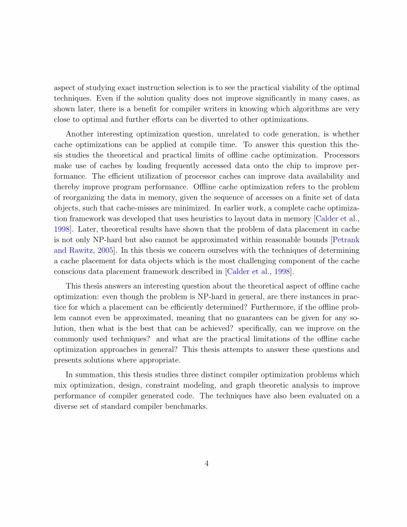
Another interesting optimization question, unrelated to code generation, is whether

cache optimizations can be applied at compile time. To answer this question this the-

sis studies the theoretical and practical limits of offline cache optimization. Processors

make use of caches by loading frequently accessed data onto the chip to improve per-

formance. The efficient utilization of processor caches can improve data availability and

thereby improve program performance. Offline cache optimization refers to the problem

of reorganizing the data in memory, given the sequence of accesses on a finite set of data

objects, such that cache-misses are minimized. In earlier work, a complete cache optimiza-

tion framework was developed that uses heuristics to layout data in memory [Calder et al.,

1998]. Later, theoretical results have shown that the problem of data placement in cache

is not only NP-hard but also cannot be approximated within reasonable bounds [Petrank

and Rawitz, 2005]. In this thesis we concern ourselves with the techniques of determining

a cache placement for data objects which is the most challenging component of the cache

conscious data placement framework described in [Calder et al., 1998].

This thesis answers an interesting question about the theoretical aspect of offline cache

optimization: even though the problem is NP-hard in general, are there instances in prac-

tice for which a placement can be efficiently determined? Furthermore, if the offline prob-

lem cannot even be approximated, meaning that no guarantees can be given for any so-

lution, then what is the best that can be achieved? specifically, can we improve on the

commonly used techniques? and what are the practical limitations of the offline cache

optimization approaches in general? This thesis attempts to answer these questions and

presents solutions where appropriate.

In summation, this thesis studies three distinct compiler optimization problems which

mix optimization, design, constraint modeling, and graph theoretic analysis to improve

performance of compiler generated code. The techniques have also been evaluated on a

diverse set of standard compiler benchmarks.

4

1.3 Thesis Organization

The rest of this thesis is organized as follows:

• Chapter 2 examines the problem of spatial and temporal scheduling for clustered

architectures. An integrated constraint programming approach is presented that

employs problem decomposition techniques for solving the two problems in tandem.

A basic model is presented which is later extended, allowing the solver to scale the

solution for practical benchmark instances. Scalability of the constraint programming

solution is also examined by comparing the performance results with traditionally

used techniques.

Some of the results in this chapter appear in the following publications.

Beg, M., and van Beek, P. 2011. A constraint programming approach to

instruction assignment. The 15th Annual Workshop on the Interaction between

Compilers and Computer Architecture (INTERACT’15). San Antonio, Texas.

Beg, M., and van Beek, P. 2013. A Constraint Programming Approach for

Integrated Spatial and Temporal Scheduling for Clustered Architectures. ACM

Transactions on Embedded Computing Systems, To appear.

• Chapter 3 studies the problem of instruction selection in code generation optimiza-

tions. This chapter presents a constraint programming model for selecting the best

sequence of machine instructions for a given program. Having presented the basic

model, an application of existing and novel enhancements to the model are introduced

for improving the performance of the solver.

• Chapter 4 starts by demonstrating that traditionally used techniques for mapping

data to cache have a fickle effect on cache performance. The improvements made by

recent cache optimizations are then examined. Furthermore, this chapter presents a

theoretical analysis of data interaction with cache utilization and presents the details

of a profile-driven approach towards cache optimization. The practical implications

of the approach are then detailed and discussed.

5

Some of the results in this chapter appear in the following publication.

Beg, M. and van Beek, P. 2010. A graph theoretic approach to cache-

conscious placement of data for direct mapped caches. In Proceedings of the

2010 International Symposium on Memory Management (ISMM ’10). Toronto,

113–120.

• Chapter 5 concludes this thesis by giving an overview of our findings and results.

In particular, this chapter discusses the practicality of the results given in the other

chapters. In addition, we also suggest areas of future research, particularly related

to cache utilization.

6

Chapter 2

Scheduling for Clustered

Architectures

Many embedded processors use clustering to scale up instruction level parallelism in a cost

effective manner. In a clustered architecture, the registers and functional units are parti-

tioned into small clusters that communicate through register-to-register copy operations.

Texas Instruments, for example, has a series of architectures for embedded processors

which are clustered. Such an architecture places a heavier burden on the compiler, which

must now assign instructions to clusters (spatial scheduling), assign instructions to cycles

(temporal scheduling), and schedule copy operations to move data between clusters. We

consider the problem of scheduling instructions in superblocks on clustered architectures

to improve performance. Scheduling for space and time is known to be a hard problem.

Previous work has proposed greedy approaches based on list scheduling to simultaneously

perform spatial and temporal scheduling, and phased approaches based on first partitioning

a block of code to do spatial assignment and then performing temporal scheduling. Greedy

approaches risk making mistakes that are then costly to recover from and partitioning ap-

proaches suffer from the well-known phase ordering problem. In this chapter, we present

a constraint programming approach for scheduling instructions on clustered architectures.

We employ a problem decomposition technique that solves spatial and temporal scheduling

in an integrated manner. We analyze the effect of different hardware parameters—such

as the number of clusters, issue-width and inter-cluster communication cost—on applica-

tion performance. We found that our approach was able to achieve an improvement of

7

up to 26%, on average, over state-of-the-art techniques on superblocks from SPEC 2000

benchmarks.

2.1 Motivation

Optimizing code for embedded processors is becoming increasingly important because of

their pervasive use in consumer electronics. For example, millions of cellular phones are

powered by members of the ARM11 processor family. Similar processors are widely used

in consumer, home and embedded applications. Their low-power and speed optimized

designs (350MHz−1GHz) make them feasible for mobile devices, media processing and

real-time applications. Billions of the ARM processors are shipped each year by various

semiconductor manufacturers [ARM, 2011].

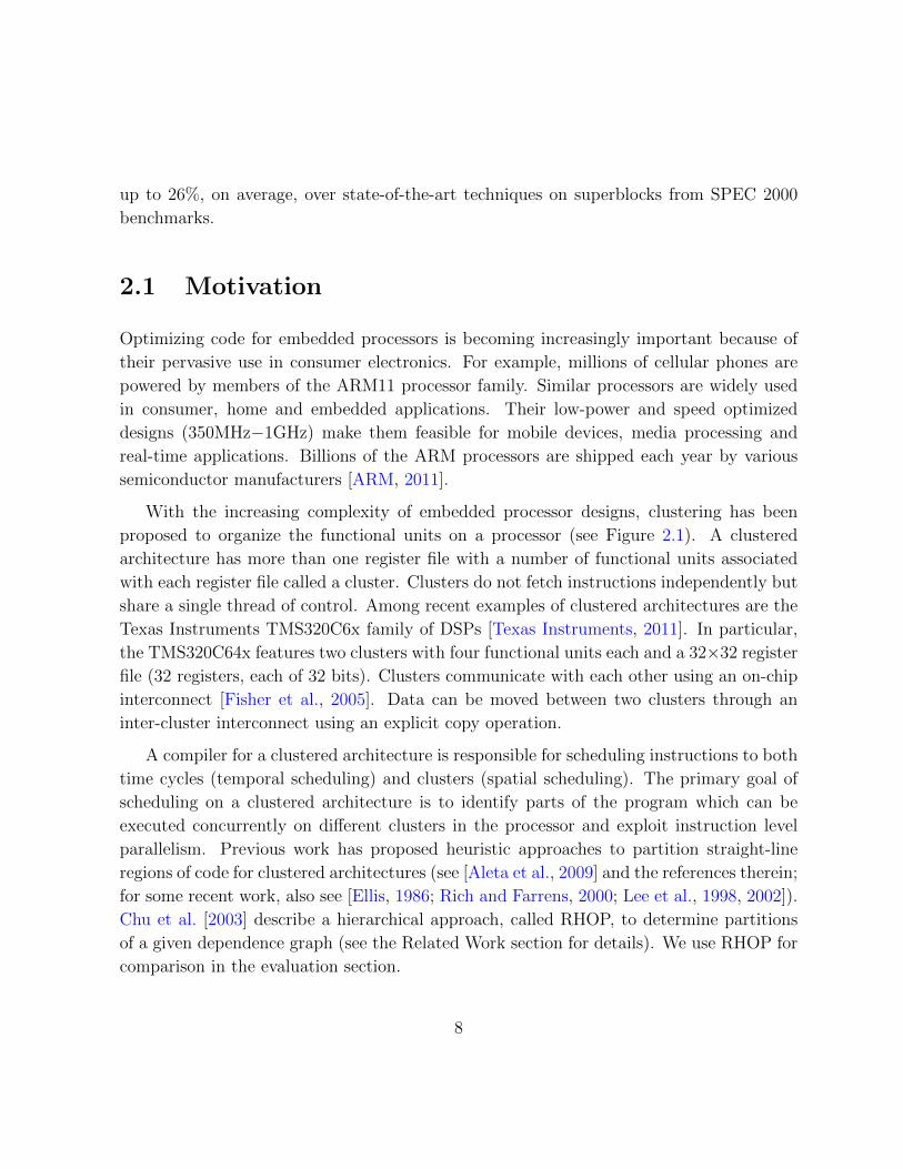
With the increasing complexity of embedded processor designs, clustering has been

proposed to organize the functional units on a processor (see Figure 2.1). A clustered

architecture has more than one register file with a number of functional units associated

with each register file called a cluster. Clusters do not fetch instructions independently but

share a single thread of control. Among recent examples of clustered architectures are the

Texas Instruments TMS320C6x family of DSPs [Texas Instruments, 2011]. In particular,

the TMS320C64x features two clusters with four functional units each and a 32×32 register

file (32 registers, each of 32 bits). Clusters communicate with each other using an on-chip

interconnect [Fisher et al., 2005]. Data can be moved between two clusters through an

inter-cluster interconnect using an explicit copy operation.

A compiler for a clustered architecture is responsible for scheduling instructions to both

time cycles (temporal scheduling) and clusters (spatial scheduling). The primary goal of

scheduling on a clustered architecture is to identify parts of the program which can be

executed concurrently on different clusters in the processor and exploit instruction level

parallelism. Previous work has proposed heuristic approaches to partition straight-line

regions of code for clustered architectures (see [Aleta et al., 2009] and the references therein;

for some recent work, also see [Ellis, 1986; Rich and Farrens, 2000; Lee et al., 1998, 2002]).

Chu et al. [2003] describe a hierarchical approach, called RHOP, to determine partitions

of a given dependence graph (see the Related Work section for details). We use RHOP for

comparison in the evaluation section.

8

Figure 2.1: Datapath model of a dual-cluster processor. The functional units are clus-

tered into two identical sets each having a separate set of registers. In the given model,

communication between clusters is through an interconnect. (Adapted from [Fisher et al.,

2005].)

In this chapter, we present a constraint programming approach for spatial scheduling

for clustered processors where clusters can communicate with each other using a cluster

interconnect with some non-zero cost. Our approach is robust and searches for an opti-

mal solution. In a constraint programming approach, a problem is modeled by stating

constraints on acceptable solutions, where a constraint defines a relation among variables,

each taking a value in a given domain. The constraint model is usually solved using back-

tracking search. The novelty of our approach lies in the decomposition of the problem and

our improvements to the constraint model in order to reduce the effort required to search

for the optimal solution. Our approach is applicable when larger compile times are accept-

able. In contrast to previous work we assume a more realistic instruction set architecture

containing non-fully pipelined and serializing instructions.

9

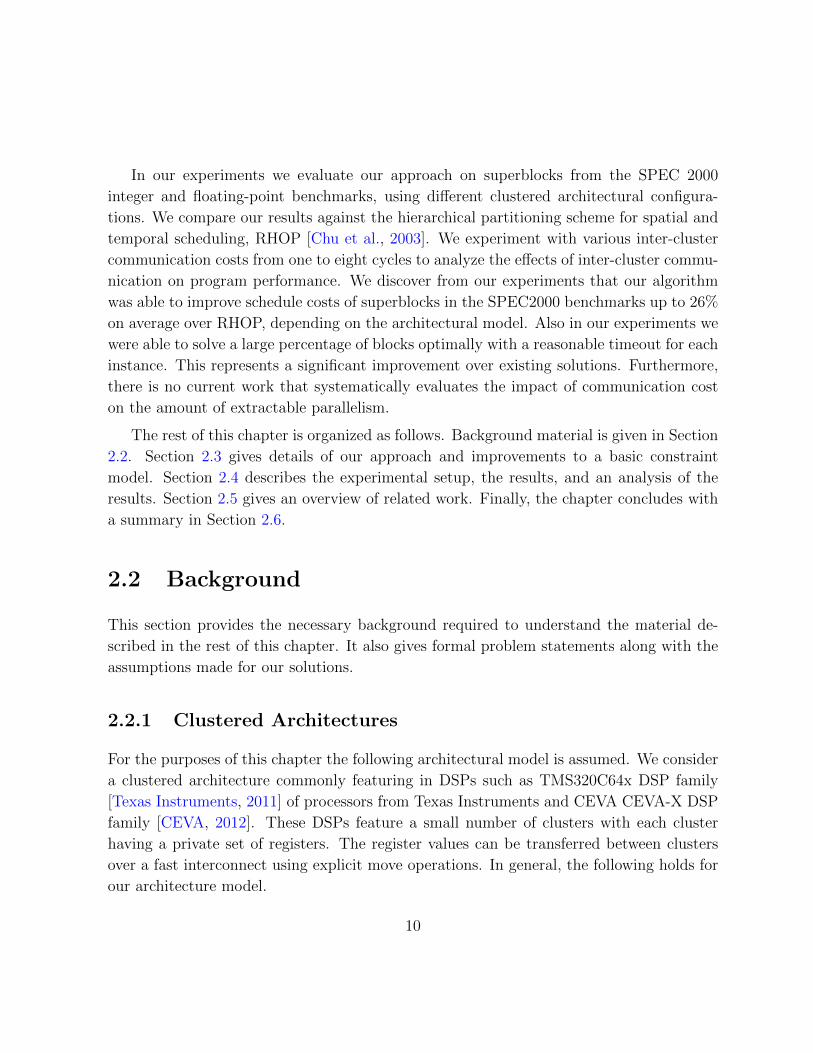
In our experiments we evaluate our approach on superblocks from the SPEC 2000

integer and floating-point benchmarks, using different clustered architectural configura-

tions. We compare our results against the hierarchical partitioning scheme for spatial and

temporal scheduling, RHOP [Chu et al., 2003]. We experiment with various inter-cluster

communication costs from one to eight cycles to analyze the effects of inter-cluster commu-

nication on program performance. We discover from our experiments that our algorithm

was able to improve schedule costs of superblocks in the SPEC2000 benchmarks up to 26%

on average over RHOP, depending on the architectural model. Also in our experiments we

were able to solve a large percentage of blocks optimally with a reasonable timeout for each

instance. This represents a significant improvement over existing solutions. Furthermore,

there is no current work that systematically evaluates the impact of communication cost

on the amount of extractable parallelism.

The rest of this chapter is organized as follows. Background material is given in Section

2.2. Section 2.3 gives details of our approach and improvements to a basic constraint

model. Section 2.4 describes the experimental setup, the results, and an analysis of the

results. Section 2.5 gives an overview of related work. Finally, the chapter concludes with

a summary in Section 2.6.

2.2 Background

This section provides the necessary background required to understand the material de-

scribed in the rest of this chapter. It also gives formal problem statements along with the

assumptions made for our solutions.

2.2.1 Clustered Architectures

For the purposes of this chapter the following architectural model is assumed. We consider

a clustered architecture commonly featuring in DSPs such as TMS320C64x DSP family

[Texas Instruments, 2011] of processors from Texas Instruments and CEVA CEVA-X DSP

family [CEVA, 2012]. These DSPs feature a small number of clusters with each cluster

having a private set of registers. The register values can be transferred between clusters

over a fast interconnect using explicit move operations. In general, the following holds for

our architecture model.

10

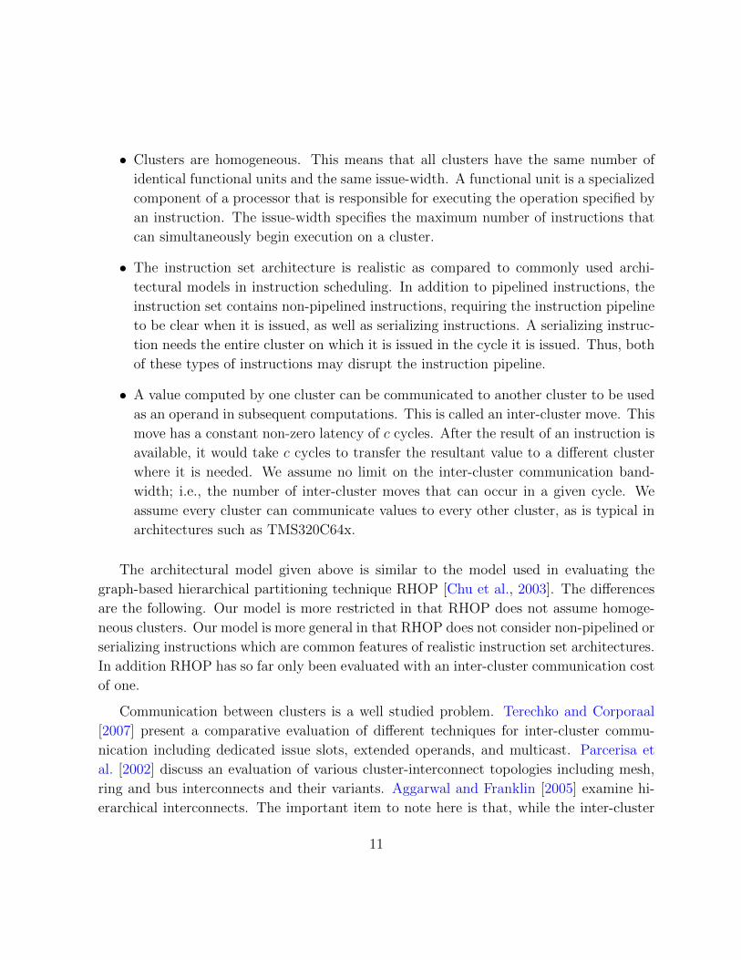
• Clusters are homogeneous. This means that all clusters have the same number of

identical functional units and the same issue-width. A functional unit is a specialized

component of a processor that is responsible for executing the operation specified by

an instruction. The issue-width specifies the maximum number of instructions that

can simultaneously begin execution on a cluster.

• The instruction set architecture is realistic as compared to commonly used archi-

tectural models in instruction scheduling. In addition to pipelined instructions, the

instruction set contains non-pipelined instructions, requiring the instruction pipeline

to be clear when it is issued, as well as serializing instructions. A serializing instruc-

tion needs the entire cluster on which it is issued in the cycle it is issued. Thus, both

of these types of instructions may disrupt the instruction pipeline.

• A value computed by one cluster can be communicated to another cluster to be used

as an operand in subsequent computations. This is called an inter-cluster move. This

move has a constant non-zero latency of c cycles. After the result of an instruction is

available, it would take c cycles to transfer the resultant value to a different cluster

where it is needed. We assume no limit on the inter-cluster communication band-

width; i.e., the number of inter-cluster moves that can occur in a given cycle. We

assume every cluster can communicate values to every other cluster, as is typical in

architectures such as TMS320C64x.

The architectural model given above is similar to the model used in evaluating the

graph-based hierarchical partitioning technique RHOP [Chu et al., 2003]. The differences

are the following. Our model is more restricted in that RHOP does not assume homoge-

neous clusters. Our model is more general in that RHOP does not consider non-pipelined or

serializing instructions which are common features of realistic instruction set architectures.

In addition RHOP has so far only been evaluated with an inter-cluster communication cost

of one.

Communication between clusters is a well studied problem. Terechko and Corporaal

[2007] present a comparative evaluation of different techniques for inter-cluster commu-

nication including dedicated issue slots, extended operands, and multicast. Parcerisa et

al. [2002] discuss an evaluation of various cluster-interconnect topologies including mesh,

ring and bus interconnects and their variants. Aggarwal and Franklin [2005] examine hi-

erarchical interconnects. The important item to note here is that, while the inter-cluster

11

communication cost is small on some popular architectures, it is not always negligible in

practical clustered architectures.

2.2.2 Instruction Scheduling

A compiler schedules instructions to take advantage of the features of the architecture and

exploit instruction level parallelism in the code. Instruction scheduling is performed on

certain regions of a program. A basic block is a region of straight-line code with a single

entry point and a single exit. A superblock is a sequence of instructions with a single entry

point and multiple possible exits. We use the directed acyclic graph (DAG) representation

for basic blocks and superblocks. In our evaluation a DAG represents a superblock. Each

vertex in the DAG corresponds to an instruction and there is an edge from vertex i to

vertex j if instruction j uses the result of instruction i. The edge is labeled with a non-

negative integer l(i, j) which represents the delay or latency between when the instruction

is issued and when the result of instruction i is available for instruction j.

The critical path distance from a vertex i to vertex j in a DAG is the maximum sum

of the latencies along any path from i to j. The earliest start time of a vertex i is a lower

bound on the earliest cycle in which the instruction i can be scheduled; i.e., the minimum

number of time cycles needed for the execution of the instructions on which i depends.

Exit vertices are special nodes in a DAG representing branch instructions in superblocks.

Each exit vertex i is associated with a weight w(i) representing the probability that the

flow of control will leave the block through this exit point. These have been calculated

through profiling. See Figure 2.2(a) for a DAG representing a superblock.

With the given architectural model and the dependency DAG for a basic block or a

superblock, the spatial scheduling problem can be described as an optimization problem

where each instruction has to be assigned to a clock cycle and also assigned to a cluster

such that the latency and resource constraints are satisfied.

Definition 2.2.1 (Temporal Schedule) A temporal schedule S for a block is a mapping

of each instruction in a DAG to a start time measured in processor clock cycles.

Definition 2.2.2 (Weighted Completion Time) The weighted completion time for a

superblock schedule is given by the summation∑n

i=1w(i)S(i), where n is the number of

12

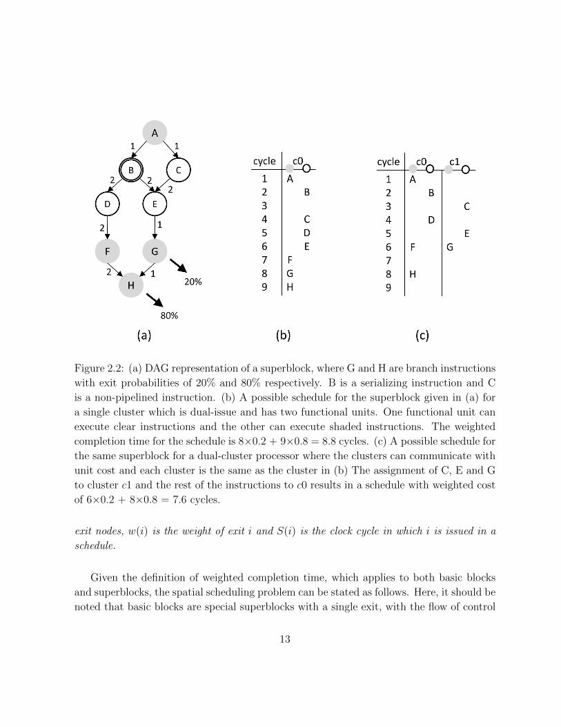
Figure 2.2: (a) DAG representation of a superblock, where G and H are branch instructions

with exit probabilities of 20% and 80% respectively. B is a serializing instruction and C

is a non-pipelined instruction. (b) A possible schedule for the superblock given in (a) for

a single cluster which is dual-issue and has two functional units. One functional unit can

execute clear instructions and the other can execute shaded instructions. The weighted

completion time for the schedule is 8×0.2 + 9×0.8 = 8.8 cycles. (c) A possible schedule for

the same superblock for a dual-cluster processor where the clusters can communicate with

unit cost and each cluster is the same as the cluster in (b) The assignment of C, E and G

to cluster c1 and the rest of the instructions to c0 results in a schedule with weighted cost

of 6×0.2 + 8×0.8 = 7.6 cycles.

exit nodes, w(i) is the weight of exit i and S(i) is the clock cycle in which i is issued in a

schedule.

Given the definition of weighted completion time, which applies to both basic blocks

and superblocks, the spatial scheduling problem can be stated as follows. Here, it should be

noted that basic blocks are special superblocks with a single exit, with the flow of control

13

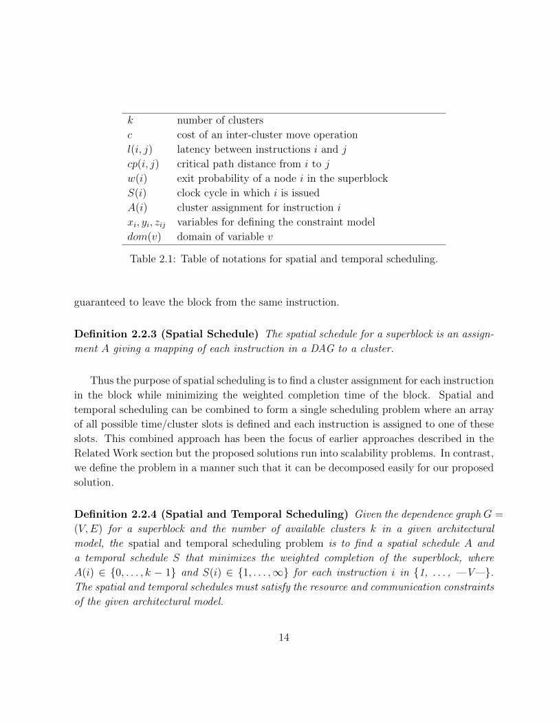
k number of clusters

c cost of an inter-cluster move operation

l(i, j) latency between instructions i and j

cp(i, j) critical path distance from i to j

w(i) exit probability of a node i in the superblock

S(i) clock cycle in which i is issued

A(i) cluster assignment for instruction i

xi, yi, zij variables for defining the constraint model

dom(v) domain of variable v

Table 2.1: Table of notations for spatial and temporal scheduling.

guaranteed to leave the block from the same instruction.

Definition 2.2.3 (Spatial Schedule) The spatial schedule for a superblock is an assign-

ment A giving a mapping of each instruction in a DAG to a cluster.

Thus the purpose of spatial scheduling is to find a cluster assignment for each instruction

in the block while minimizing the weighted completion time of the block. Spatial and

temporal scheduling can be combined to form a single scheduling problem where an array

of all possible time/cluster slots is defined and each instruction is assigned to one of these

slots. This combined approach has been the focus of earlier approaches described in the

Related Work section but the proposed solutions run into scalability problems. In contrast,

we define the problem in a manner such that it can be decomposed easily for our proposed

solution.

Definition 2.2.4 (Spatial and Temporal Scheduling) Given the dependence graph G =

(V,E) for a superblock and the number of available clusters k in a given architectural

model, the spatial and temporal scheduling problem is to find a spatial schedule A and

a temporal schedule S that minimizes the weighted completion of the superblock, where

A(i) ∈ {0, . . . , k − 1} and S(i) ∈ {1, . . . ,∞} for each instruction i in {1, . . . , —V—}.The spatial and temporal schedules must satisfy the resource and communication constraints

of the given architectural model.

14

Temporal scheduling on realistic multiple issue processors is known to be NP-hard and

compilers use heuristic approaches to schedule instructions. On clustered architectures

the compiler has an additional task of spatial scheduling, partitioning instructions across

the available computing resources. The compiler has to carefully consider the tradeoffs

between parallelism and locality because a small mistake in spatial scheduling is more

costly than a small mistake in temporal scheduling. For example, if a critical instruction is

scheduled one cycle late then only a single cycle is lost. But if the same is scheduled on a

different cluster then multiple cycles may be lost from unnecessary communication delays

and resource contention. The combination of spatial and temporal scheduling is a much

harder problem than the temporal scheduling problem. In our approach we partition the

DAG and schedule each partition on a cluster. To overcome the well-known phase ordering

problem; i.e. determining the order in which a particular set of optimizations should be

applied, we backtrack over the possible partitions, searching for a partition that leads to an

optimal schedule. The distinguishing feature of our solution is the collection of techniques

for accelerating the search which makes our approach useful in practice.

Definition 2.2.5 (Balanced Graph Partitioning) The balanced graph partitioning prob-

lem consists of splitting a graph G into k disjoint components of roughly equal size such

that the number of edges between different components is minimized.

When k = 2, the problem is also referred to as the graph bisection problem. Balanced

graph partitioning is known to be NP-hard for k ≥ 2 [Andreev and Racke, 2004]. In

practice, however, the spatial scheduling problem described above can be even harder than

balanced graph partitioning because the optimal partitions of the DAG can also be fewer

than k (so it would need to consider solutions with number of partitions from 1 to k).

2.2.3 Constraint Modeling

We use constraint programming to model and solve the integrated spatial and temporal

scheduling problem. Constraint programming is a methodology for solving hard combina-

torial problems, where a problem is modeled in terms of variables, values and constraints

(see [Rossi et al., 2006]).

15

Definition 2.2.6 (Constraint Model) A constraint model consists of a finite set of

variables X = {x1, · · · , xn}, a finite domain of values dom(xi) that each variable xi ∈ Xcan take and a set of constraints C = {C1, · · · , Cm} where each constraint is defined over

a subset of variables in X. A solution to the constraint model is an assignment of a value

to each variable in X such that all of the constraints in C are satisfied.

Once the problem has been modeled such that the variables along with their domains

have been identified and the constraints specified, backtracking over the variables is em-

ployed to search for a solution. At every stage of the backtracking search, there is some

current partial solution that the algorithm attempts to extend to a full solution by as-

signing a value to an uninstantiated variable. One of the reasons behind the success of

constraint programming is the idea of constraint propagation. During the backtracking

search when a variable is assigned a value, the constraints are used to reduce the domains

of the uninstantiated variables by ensuring that the values in their domains are consistent

with the constraints. Given sufficient time the constraint programming backtracking ap-

proach is guaranteed to find a solution if one exists. If running time is a constraint, then

the solver uses a timeout for the search algorithm and returns the best solution that was

found before search is terminated without any guarantees for the quality of the solution.

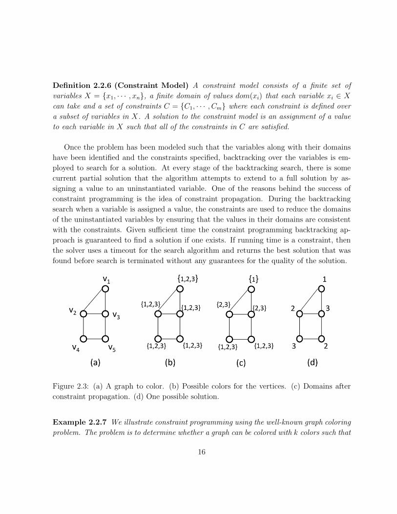
Figure 2.3: (a) A graph to color. (b) Possible colors for the vertices. (c) Domains after

constraint propagation. (d) One possible solution.

Example 2.2.7 We illustrate constraint programming using the well-known graph coloring

problem. The problem is to determine whether a graph can be colored with k colors such that

16

adjacent vertices are assigned different colors. In one possible constraint formulation of the

problem there is a variable for each vertex, v1, . . ., vn, the domains of the variables are the

possible colors {1, . . . , k} and the binary constraints are that two adjacent vertices should

not have the same color; i.e., vi 6= vj if vi and vj are adjacent. Consider the constraint

formulation for the graph with five vertices shown in Figure 2.3(a), where k is 3. Each of

the five vertices can be assigned one of the three colors {1, 2, 3}. In constraint programming,

instantiating one of the variables, such as v1 to 1 adds an additional constraint to the model

and results in the removal of some values from the domains of some other variables; i.e.,

v2 and v3 can no longer be assigned the color 1. This is called constraint propagation (see

Figure 2.3(b)). A partial solution is consistent if the values in the domains of variables

have support. A value having support means that it can be a part of a solution given the

set of constraints. For example, given that v1 is 1, the color 1 no longer has support in v2.

Backtracking search traverses the search tree by examining alternate values for the variables

in the constraint model in order to find a solution. Backtracking algorithms maintain a

level of consistency using constraint propagation.

2.3 Constraint Programming Approach

In this section we present a constraint model for the spatial scheduling problem. A block

of code given by either a basic block or superblock is represented by a DAG where each

node is an instruction and the edges represent the dependency between instructions. Each

node i in the graph is represented by two variables in the model, xi and yi. The variable

xi ∈ {1, . . . ,m} is the temporal variable representing the cycle in which the instruction is

to be issued. The upper-bound m to these variables can be calculated using a heuristic

scheduling method for a single cluster. The variable yi ∈ {0, . . . , k − 1} is the spatial

variable that identifies the cluster to which instruction i is to be assigned. The key is to

scale up to large problem sizes. In developing an optimal solution to the spatial schedul-

ing problem we have applied and adapted several techniques from the literature including

symmetry breaking, branch and bound [Rossi et al., 2006] and structure based decompo-

sition techniques [Benders, 1962]. It should be noted here that spatial scheduling cannot

be feasibly and reliably solved independently as it heavily relies on temporal scheduling to

determine the cost of a given cluster assignment. This leads us to an integrated solution

design.

17

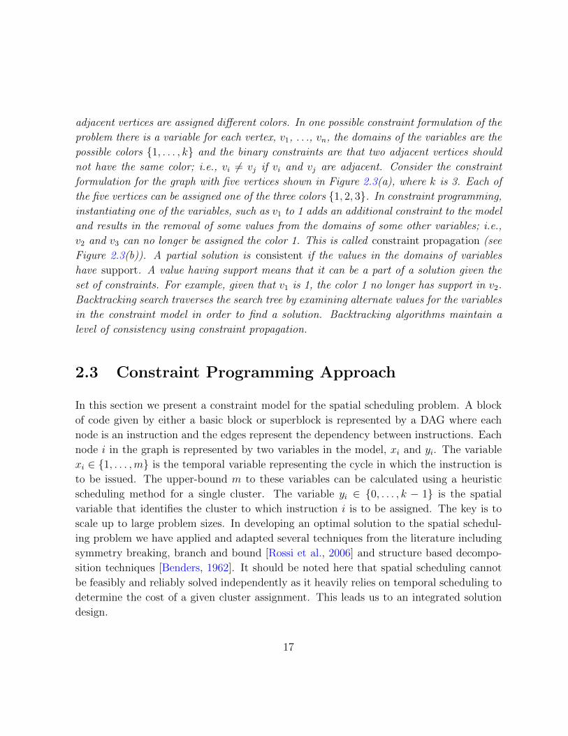
Figure 2.4: (a) Example basic block. (b) Search tree for the simple constraint model

associated with the basic block. Each level in the search tree corresponds to assigning a

value to a variable; i.e., a partial solution is constructed. For example, at a depth of one,

the assignment yA = 0 corresponds to assigning instruction A to cluster 0. At a leaf, all of

the variables have been assigned.

The main technique is to solve the problem using a master-slave decomposition which

preserves optimality makes our solution scale to large problem sizes. We solve spatial

scheduling as the master problem. Once a probable spatial schedule is determined the

temporal scheduler solves for the optimal schedule of instructions for the given cluster

assignment. The master problem determines the assignment to the y variables (i.e., the

cluster assignment to each instruction) and the slave problem schedules each instruction

to a time cycle.

Example 2.3.1 (Example Basic Block) Figure 2.4(a) shows a simple dependency DAG

for a basic block. The search tree for a simple constraint model for a 4-cluster architecture

is shown in Figure 2.4(b) where the assignment of each instruction to a cluster is deter-

mined at the leaf nodes and the optimal scheduler is used to calculate the temporal schedule

for the given assignment. We use this as our running example.

18

The design of our solution was inspired by [Benders, 1962] and [Dantzig and Wolfe, 1960]

decomposition techniques in integer programming, where an integer program is decomposed

into a master-slave problem and the master problem generates many subproblems (or slave

problems) which are solved hierarchically.

2.3.1 Symmetry Breaking

Symmetry can be exploited to reduce the amount of search needed to solve the problem.

Backtracking over symmetric states does not improve the solution and consumes valuable

computation time. If the search algorithm is repeatedly visiting similar states then rec-

ognizing and excluding equivalent states can significantly reduce the size of the search

space. Using the technique of symmetry breaking, we aim to remove provably symmetric

assignments to instructions. An example of symmetry breaking would be assigning the

first instruction to the first cluster and thus discarding all the solutions where the first in-

struction is on any other cluster. This approach guarantees the preservation of at least one

optimal assignment. This is because only redundant solutions are removed from the search.

Thus, an optimal solution is removed using symmetry breaking only if an equivalent but

symmetric solution has been evaluated earlier.

Our approach to symmetry breaking is to reformulate the problem such that the algo-

rithm does not revisit symmetric states repeatedly. We model the problem such that each

edge (vi, vj) in the DAG is represented by a variable zij ∈ {=, 6=}. The z variables are

introduced to express whether a pair of instructions should be executed on the same clus-

ter or on different clusters. Our model inherently breaks symmetry by using backtracking

search to assign values to the z variables, which represent the edges in the blocks. For a

variable zij, assigning a value of = means that variables yi and yj must take the same value

and assigning a value of 6= means that yi and yj must take different values.

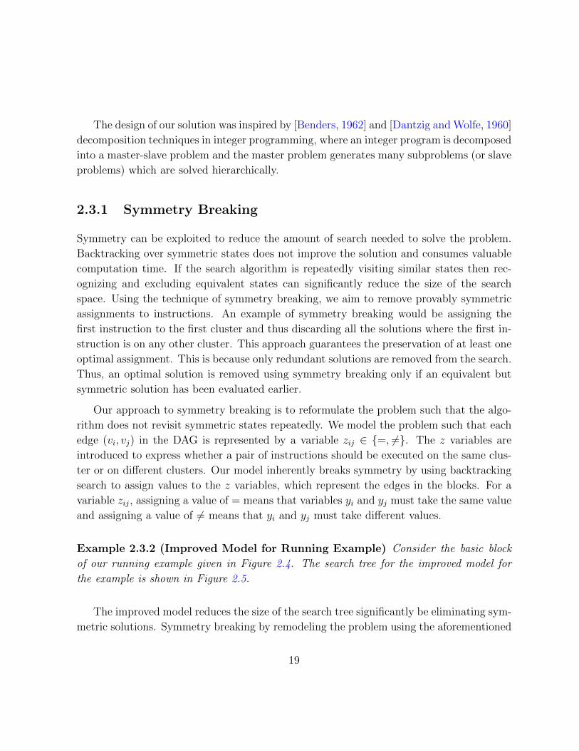
Example 2.3.2 (Improved Model for Running Example) Consider the basic block

of our running example given in Figure 2.4. The search tree for the improved model for

the example is shown in Figure 2.5.

The improved model reduces the size of the search tree significantly be eliminating sym-

metric solutions. Symmetry breaking by remodeling the problem using the aforementioned

19

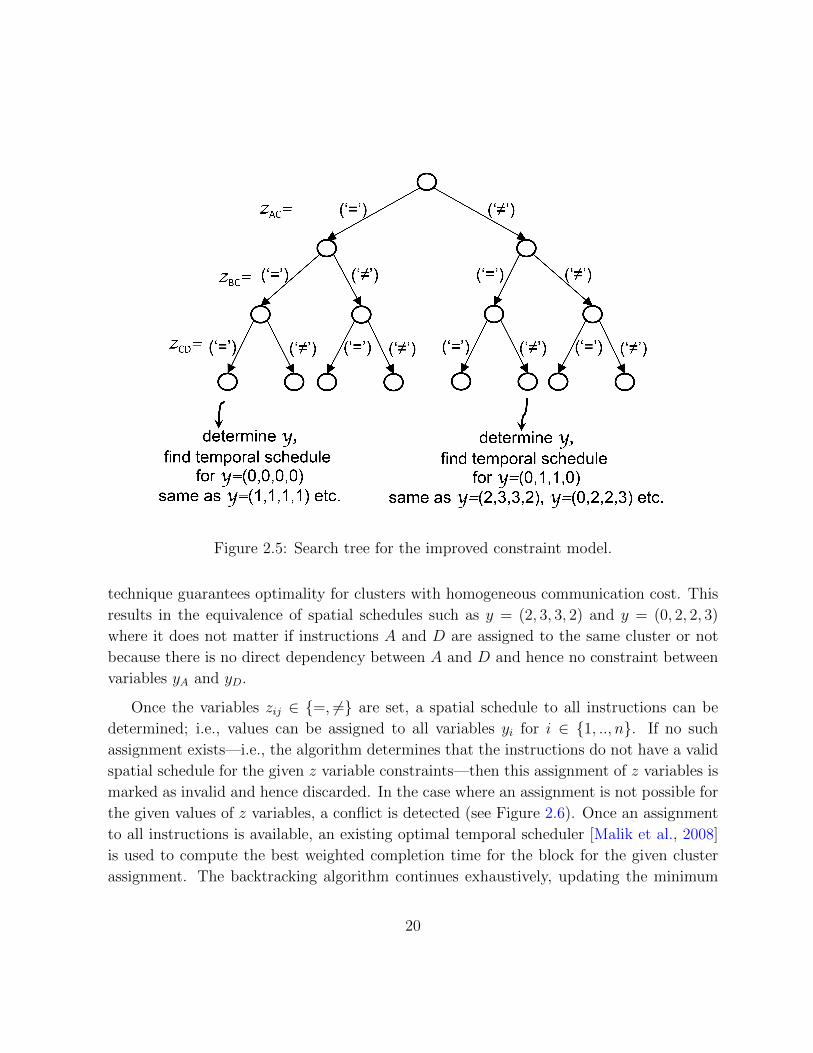
Figure 2.5: Search tree for the improved constraint model.

technique guarantees optimality for clusters with homogeneous communication cost. This

results in the equivalence of spatial schedules such as y = (2, 3, 3, 2) and y = (0, 2, 2, 3)

where it does not matter if instructions A and D are assigned to the same cluster or not

because there is no direct dependency between A and D and hence no constraint between

variables yA and yD.

Once the variables zij ∈ {=, 6=} are set, a spatial schedule to all instructions can be

determined; i.e., values can be assigned to all variables yi for i ∈ {1, .., n}. If no such

assignment exists—i.e., the algorithm determines that the instructions do not have a valid

spatial schedule for the given z variable constraints—then this assignment of z variables is

marked as invalid and hence discarded. In the case where an assignment is not possible for

the given values of z variables, a conflict is detected (see Figure 2.6). Once an assignment

to all instructions is available, an existing optimal temporal scheduler [Malik et al., 2008]

is used to compute the best weighted completion time for the block for the given cluster

assignment. The backtracking algorithm continues exhaustively, updating the minimum

20

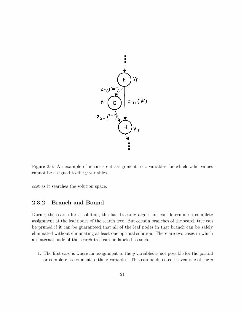
Figure 2.6: An example of inconsistent assignment to z variables for which valid values

cannot be assigned to the y variables.

cost as it searches the solution space.

2.3.2 Branch and Bound

During the search for a solution, the backtracking algorithm can determine a complete

assignment at the leaf nodes of the search tree. But certain branches of the search tree can

be pruned if it can be guaranteed that all of the leaf nodes in that branch can be safely

eliminated without eliminating at least one optimal solution. There are two cases in which

an internal node of the search tree can be labeled as such.

1. The first case is where an assignment to the y variables is not possible for the partial

or complete assignment to the z variables. This can be detected if even one of the y

21

variables cannot be assigned a value in {0, ..., k−1} without violating the constraints

given by the z variables. An example of such a violation is given in Figure 2.6. In

the example, consider instructions F and G. Since zFG is = they are assigned to

the same cluster, say c0. Now H cannot be correctly assigned to either c0 or any

other cluster since yH should be different from yF but the same as yG which is not

possible. To discover such violations early in the search, the z variables are assigned

in a fixed order that corresponds to a breadth-first traversal of the DAG. Breadth-

first traversal detects triangular patterns such as the ones given in Figure 2.6 faster

than other possible orderings such as depth-first.

2. The second case is where the partial assignment to the y variables can be proven

to only result in a temporal schedule with a cost greater than the established upper

bound. Proving that such a case holds is done by adding the cost of the temporal

schedule of the instructions assigned to clusters with a lower bound on the cost

of a temporal schedule of the instructions not yet assigned to clusters. Thus, any

assignment that contains the given subset of cluster assignment cannot result in

a better temporal schedule. The search space can be reduced by eliminating all

such assignments containing this sub-assignment. Also note that the upper bound is

gradually improved upon as better solutions are found.

In both the above mentioned cases the backtracking algorithm does not descend further

in the search tree. Branch and bound continuously prunes the search during the execution

of the algorithm as upper-bounds are improved upon.

2.3.3 Connected Structures

The amount of search done by the algorithm can be reduced if it can be pre-determined

that a subset of instructions in a block are tightly coupled and would be assigned to the

same cluster in at least one optimal solution to the scheduling problem. Recall that the

earliest start time of an instruction is the earliest possible cycle in which an instruction

can be issued. Given a set C of such instructions in a block, an outgoing edge e is an edge

for which one of the nodes connected to e is in C and the other one is not in C. Similarly,

an incoming edge is an edge from an instruction on which the current instruction depends.

Using these definitions we define a connected structure as follows.

22

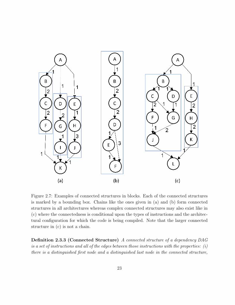
Figure 2.7: Examples of connected structures in blocks. Each of the connected structures

is marked by a bounding box. Chains like the ones given in (a) and (b) form connected

structures in all architectures whereas complex connected structures may also exist like in

(c) where the connectedness is conditional upon the types of instructions and the architec-

tural configuration for which the code is being compiled. Note that the larger connected

structure in (c) is not a chain.

Definition 2.3.3 (Connected Structure) A connected structure of a dependency DAG

is a set of instructions and all of the edges between those instructions with the properties: (i)

there is a distinguished first node and a distinguished last node in the connected structure,

23

where first and last is determined by considering the edges in the connected structure as a

partial order; (ii) there is a path from the first node to the last node; (iii) all incoming edges

are incident with the first node; (iv) all outgoing edges are incident with the last node; and

(v) the set of instructions can be scheduled on a single cluster such that the latency and

resource constraints are satisfied and each instruction can be scheduled at its earliest start

time.

The definition implies that the given set of instructions in a connected structure, if

considered separately, cannot have a better schedule even if there are more functional

units in the cluster or if there are more clusters. Some examples of connected structures

are given in Figure 2.7. For example, in Figure 2.7(a) the three connected structures in

the block are identified with boxes form chains. A chain is a totally ordered set of three

or more instructions in the dependency DAG.

Lemma 2.3.4 A chain is a connected structure in our architectural model.

Proof: A chain consists of a set of totally ordered instructions which means that the

second instruction in the chain cannot be executed until the result of the first is avail-

able. Similarly, the third instruction cannot begin execution until the second instruction

has completed execution and so forth. The simplest architectural model is a single issue

clustered architecture having a single functional unit. The instructions in the chain can

be executed on this functional unit one by one. Now consider that the number of func-

tional units on this cluster are increased along with the issue-width. There is no better

schedule for the chain compared to the previous architecture since there is no instruction

level parallelism (ILP) that can be exploited by extending the architecture. Similarly, if

we increase the number of clusters, there is no more ILP that can be exploited by the

additional clusters. Hence the number of cycles required to execute the chain remain the

same regardless of the architectural model. �

Once the connected structures in a superblock have been identified, the superblock

can be decomposed if there are no dependency edges between these structures and each in-

struction, other than distinguished source and sink nodes, belongs to a connected structure.

For example, all of the superblocks shown in Figure 2.7 are decomposable into connected

structures.

24

Theorem 2.3.5 Given a superblock that can be decomposed into one or more chains, if the

number of chains is less than or equal to the number of available clusters, the instructions

within each chain can be assigned to the same cluster without eliminating at least one

optimal assignment of the instructions to clusters.

Proof: By Definition 2.3.3, each instruction in a chain can be scheduled at its earliest start

time. As the number of chains is less than or equal to the number of available clusters, no

instruction can be issued earlier than the resulting schedule. �

For the purpose of the experiments reported in this chapter we only consider chains as

connected structures. The solver still finds the optimal solution but recognizing the non-

chain connected structures would have reduced the amount of search needed to compute

the solution.

2.3.4 Solving an Instance

Given an architectural model which consists of the number of clusters k, the communication

cost c, the issue width, and the number and type of the functional units, solving an instance

of the spatial scheduling problem proceeds with the following steps (see Algorithm 1). First,

a constraint model for edge assignment is constructed. The lower-bound and the upper-

bound on the cost of the schedule on the given number of clusters is established. The

lower-bound is computed using the optimal temporal scheduler [Malik et al., 2008]. To

compute the lower-bound for the given clustered architectural model, we schedule for a

simpler architecture that has no serializing instructions and a single cluster. The single

cluster has the same total number and types of functional units as all of the clusters in

the given architectural model combined. Effectively this simulates a communication cost

of zero between clusters and gives us a lower bound on the true cost of the schedule. The

upper-bound is initially established using an extension to the list-scheduling algorithm.

The extension to the list scheduler consists of a fast greedy heuristic to assign superblock

instructions to clusters. The algorithm greedily assigns instructions to clusters as soon as

the dependency, resource and communication constraints are satisfied. These sophisticated

methods are employed to compute tight lower and upper bounds so that the algorithm does

not spend valuable compile time in search. The lower and upper-bounds are passed on to

the backtracking algorithm along with the constraint model.

25

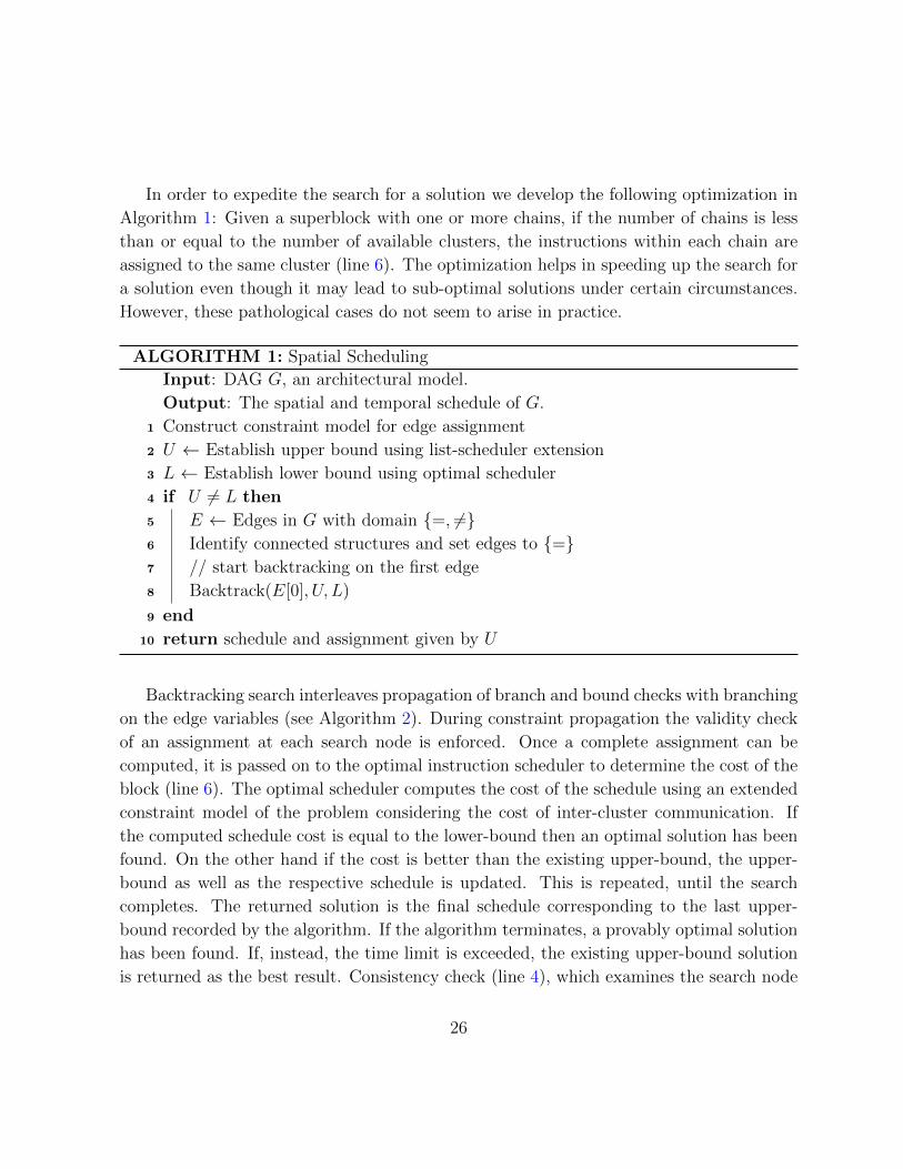
In order to expedite the search for a solution we develop the following optimization in

Algorithm 1: Given a superblock with one or more chains, if the number of chains is less

than or equal to the number of available clusters, the instructions within each chain are

assigned to the same cluster (line 6). The optimization helps in speeding up the search for

a solution even though it may lead to sub-optimal solutions under certain circumstances.

However, these pathological cases do not seem to arise in practice.

ALGORITHM 1: Spatial Scheduling

Input: DAG G, an architectural model.

Output: The spatial and temporal schedule of G.

1 Construct constraint model for edge assignment

2 U ← Establish upper bound using list-scheduler extension

3 L ← Establish lower bound using optimal scheduler

4 if U 6= L then

5 E ← Edges in G with domain {=, 6=}6 Identify connected structures and set edges to {=}7 // start backtracking on the first edge

8 Backtrack(E[0], U, L)

9 end

10 return schedule and assignment given by U

Backtracking search interleaves propagation of branch and bound checks with branching

on the edge variables (see Algorithm 2). During constraint propagation the validity check

of an assignment at each search node is enforced. Once a complete assignment can be

computed, it is passed on to the optimal instruction scheduler to determine the cost of the

block (line 6). The optimal scheduler computes the cost of the schedule using an extended

constraint model of the problem considering the cost of inter-cluster communication. If

the computed schedule cost is equal to the lower-bound then an optimal solution has been

found. On the other hand if the cost is better than the existing upper-bound, the upper-

bound as well as the respective schedule is updated. This is repeated, until the search

completes. The returned solution is the final schedule corresponding to the last upper-

bound recorded by the algorithm. If the algorithm terminates, a provably optimal solution

has been found. If, instead, the time limit is exceeded, the existing upper-bound solution

is returned as the best result. Consistency check (line 4), which examines the search node

26

ALGORITHM 2: BacktrackInput: E[i] the current edge, architectural model, an upper bound on the

schedule cost U , and a lower bound on the schedule cost L.

Output: Spatial and temporal schedule associated with U .

1 for all values that can be assigned to the current edge do

2 n← search node corresponding to the current assignment of variables

3 if n is a leaf node of search tree then

4 if ConsistencyCheck( n ) then

5 A ← generate assignment for n

6 S ← determine schedule for assignment A

7 U ← Update(U) using S

8 end

9 end

10 if n is an internal node of search tree then

11 if ConsistencyCheck( n ) && BoundsCheck( n ) then

12 // continue onto the next edge

13 Backtrack(E[i+ 1], U, L)

14 end

15 end

16 if U = L then

17 return A, S for the upper bound U as solution

18 end

19 end

20 return A, S for the upper bound U as solution

for the first case in sub-section 2.3.2 and bounds check (line 11) are intended to prune

the search tree and save computation time. The following step-by-step execution on the

running example provides a better description of the algorithms.

Example 2.3.6 (Solving the Running Example) Consider the basic block DAG from

our running example given in Figure 2.4(a) on a 4-cluster 1-issue architecture with inter-

cluster communication cost of 1. Spatial scheduling (Algorithm 1) proceeds by creating a

constraint model. Determining the upper bound U on the schedule length yields 4 (i.e.,

27

U ← 4) and lower bound (L) is determined to be 3 (L← 3). Since there are no connected

structures in the DAG, the algorithm proceeds by backtracking on the edges (AC,BC and

CD). Algorithm 2 iteratively assigns {=, 6=} to the z variables. For example, initially zAC

is assigned =. Then a consistency check is run to make sure that it is possible to assign

the y variables valid values if zAC ←= constraint is added to the model. This corresponds

to the first case in subsection 2.3.2. Since the current search node (n) is an internal node

of the search tree (corresponding to the left child of the root in the search tree shown in

Figure 2.5) the second condition starting at line 10 is executed. It runs a bounds check

on n which computes a lower bound for a partial assignment (which is 2) where yA = yCmaking sure that it does not exceed U . Backtracking continues recursively on the edges.

Consider the search node where {zAC ←=, zBC ←6=, zCD ←=}. The algorithm finds it to

be consistent, generates an assignment (0,1,0,0), and determines the optimal schedule for

the given spatial assignment (lines 5, 6). The optimal scheduler uses an extended model

with the inter-cluster communication constraints for instructions which are scheduled on

different clusters. The condition on line 16 determines that since U = L the assignment is

an optimal solution and hence returns it without searching the entire tree.

2.4 Experimental Evaluation

In this section, we present an empirical evaluation of our scheduler for clustered architec-

tures.

2.4.1 Experimental Setup

We evaluated our integrated solution to the spatial and temporal scheduling problem on

superblocks from the SPEC 2000 integer and floating point benchmarks. Our approach

is equally applicable to basic blocks, but we present only the results for superblocks as

these consistently show better improvements than the basic blocks. Our approach per-

forms better on the superblocks because superblocks are more complex and hence more

challenging to schedule for heuristic approaches. Also, our constraint programming so-

lution has a global view of the problem as compared to heuristic approaches which tend

to have a local view. The benchmark suite consists of source code for software packages

chosen to represent a variety of programming languages and types of applications. The

28

results given in this chapter are for superblocks. The benchmarks were compiled using the

IBM Tobey compiler [Blainey, 1994] targeted towards the PowerPC processor [Hoxey et

al., 1996], and the superblocks were captured as they were passed to Tobey’s instruction

scheduler. The compiler also marks serializing instructions and non-pipelined instructions.

Note that on the PowerPC, for example, 15% of the instructions in the superblocks are

serializing instructions.

issue width integer units memory units branch units floating point units

1-issue 1

2-issue 1 1 1 1

4-issue 2 1 1 1

Table 2.2: Architectural models and their composition in terms of the number and types

of functional units.

The compilations were done using Tobey’s highest level of optimization, which includes

aggressive optimization techniques such as software pipelining and loop unrolling. The

Tobey compiler performs instruction scheduling once before global register allocation and

once again afterward. Spatial scheduling is performed on the superblocks after register

allocation. The results given are for the most frequently executed superblocks in the

benchmarks—superblocks that executed at least 100,000 times during profiling. Experi-

ments were also performed that included less frequently executed superblocks (not shown)

but the overall results were qualitatively similar. Following Faraboschi et al. [1998], in the

experiments we present our results relative to a baseline configuration which is an archi-

tecture with a single cluster having the same number of functional units and same issue

width as a single cluster in the multi-cluster configuration being experimented with.

We compare against two versions of the graph-based hierarchical partitioning tech-

nique RHOP [Chu et al., 2003] (see Related Work, Section 2.5 for a detailed description

of RHOP). The first version of RHOP—a reimplementation of the version that appears in

the Trimaran compiler [Chakrapani et al., 2009]—uses a regular list scheduler for instruc-

tion scheduling (denoted here as rhop-ls). The second version of RHOP uses an optimal

instruction scheduler [Malik et al., 2008] (denoted here as rhop-opt).

We conducted our evaluation using the three architectural models which are similar

to real clustered architectures. The configuration for each cluster is shown in Table 2.2.

29

We experimented with 2-8 fully connected, homogeneous clusters [Terechko, 2007] with

issue widths ranging from 1 to 4 on each cluster. In these architectures, the functional

units are not fully pipelined, the issue width of the cluster is not always equal to the

number of functional units, and there are serializing instructions. We run our experiments

for homogeneous clusters; i.e., all clusters have exactly the same number and type of

functional units. Additionally, clusters can communicate with each other with a non-

zero latency. In our model, communication between clusters happens via an inter-cluster

interconnect which is an explicit copy operation. A realistic communication model has a

4-cycle latency on a four cluster and 6-cycles on an eight cluster processor [Parcerisa et

al., 2002]. We also study the impact of various communication latencies on performance.

We measure the speedup by computing the cycle count improvements over the baseline.

The experiments were run on the whale cluster of the Sharcnet systems (www.sharcnet.ca).

Each node of the whale cluster is equipped with four Opteron CPUs at 2.2 GHz and 4.0 GB

memory.

2.4.2 Experimental Results & Analysis

In this section we present the results of our experiments. We structure the presentation

of the results and our analysis as follows. First, we perform a general comparison of

our constraint-programming-based integrated spatial and temporal scheduler, referred to

as cp, with two versions of RHOP: RHOP using the regular list scheduler for scheduling

(rhop-ls) and RHOP using the optimal instruction scheduler (rhop-opt), which is also

being used by our algorithm. Second, we perform a detailed comparison that examines the

impact of the number of clusters on the performance of the algorithms. Third, we perform

a detailed comparison that examines the impact of the communication cost due to the

different cluster-interconnect topologies on the performance of the algorithms. Finally, as

our integrated scheduler is more costly in terms of scheduling time, we examine the time

taken to schedule the superblocks in the various benchmarks.

A general comparison of our integrated spatial and temporal scheduler with RHOP. In

Figures 2.8 and 2.9 we present detailed performance results for the constraint programming

algorithm cp as compared to the two flavors of the RHOP algorithm, rhop-ls and rhop-

opt where rhop-ls is the original approach presented in [Chu et al., 2003] and that our

results for rhop-ls closely match the experimental results presented therein. We include

rhop-opt to factor out the contribution of the optimal instruction scheduler and examine

30

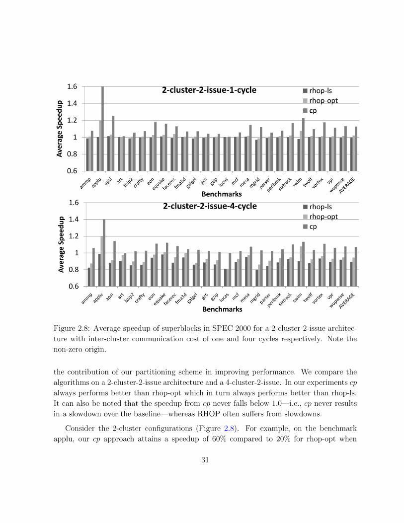
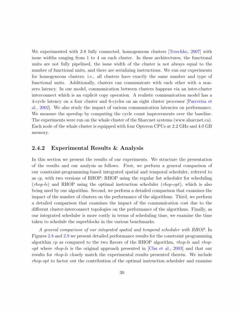
Figure 2.8: Average speedup of superblocks in SPEC 2000 for a 2-cluster 2-issue architec-

ture with inter-cluster communication cost of one and four cycles respectively. Note the

non-zero origin.

the contribution of our partitioning scheme in improving performance. We compare the

algorithms on a 2-cluster-2-issue architecture and a 4-cluster-2-issue. In our experiments cp

always performs better than rhop-opt which in turn always performs better than rhop-ls.

It can also be noted that the speedup from cp never falls below 1.0—i.e., cp never results

in a slowdown over the baseline—whereas RHOP often suffers from slowdowns.

Consider the 2-cluster configurations (Figure 2.8). For example, on the benchmark

applu, our cp approach attains a speedup of 60% compared to 20% for rhop-opt when

31

Figure 2.9: Average speedup of superblocks in SPEC 2000 for a 4-cluster 2-issue architec-

ture with inter-cluster communication cost of one and four cycles respectively. Note the

non-zero origin.

the inter-cluster communication cost is one cycle, a performance gap of 40%, and our

cp approach attains a speedup of 40% compared to 20% for rhop-opt when the inter-

cluster communication cost is four cycles, a performance gap of 20%. On average across

all 26 benchmarks the performance gap between cp and rhop-opt is close to 15% when the

communication cost is one cycle and approximately 10% when the communication cost is

four cycles.

32

1 3

1.5

1.7

up

average‐2‐cycle rhop‐lsrhop‐optcp

1 3

1.5

1.7

up

average‐1‐cycle rhop‐lsrhop‐optcp

0.9

1.1

1.3

verage Spe

edu

0.9

1.1

1.3

verage Spe

edu

0.5

0.7

0.9

Av

0.5

0.7

0.9

Av

2―1, 4―1, 8―1 2―2, 4―2, 8―2 2―4, 4―4, 8―4

Architectural Model1.7

average‐4‐cycle rhop‐lsrhop opt

1.7average‐8‐cycle rhop‐ls

rhop opt

2―1, 4―1, 8―1 2―2, 4―2, 8―2 2―4, 4―4, 8―4

Architectural Model

1 1

1.3

1.5

Speedu

p

rhop‐optcp

1 1

1.3

1.5Speedu

prhop‐optcp

0.7

0.9

1.1

Average S

0.7

0.9

1.1

Average S

0.52―1,4―1, 8―1 2―2,4―2, 8―2 2―4,4―4, 8―4

Architectural Model

0.52―1, 4―1, 8―1 2―2, 4―2, 8―2 2―4, 4―4, 8―4

Architectural Model

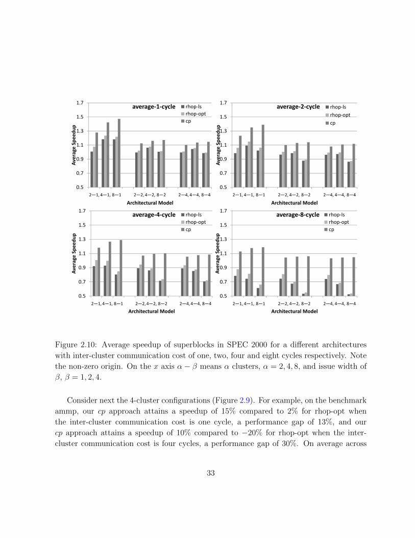
Figure 2.10: Average speedup of superblocks in SPEC 2000 for a different architectures

with inter-cluster communication cost of one, two, four and eight cycles respectively. Note

the non-zero origin. On the x axis α− β means α clusters, α = 2, 4, 8, and issue width of

β, β = 1, 2, 4.

Consider next the 4-cluster configurations (Figure 2.9). For example, on the benchmark

ammp, our cp approach attains a speedup of 15% compared to 2% for rhop-opt when

the inter-cluster communication cost is one cycle, a performance gap of 13%, and our

cp approach attains a speedup of 10% compared to −20% for rhop-opt when the inter-

cluster communication cost is four cycles, a performance gap of 30%. On average across

33

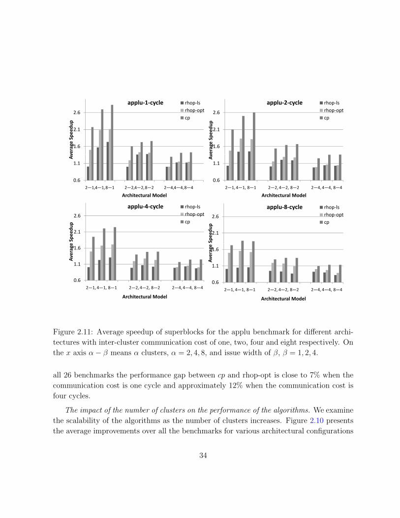
2.6

up

applu‐1‐cycle rhop‐lsrhop‐optcp

2.6

up

applu‐2‐cycle rhop‐lsrhop‐optcp

1.6

2.1

verage Spe

edu

1.6

2.1

verage Spe

edu

0.6

1.1

Av

0.6

1.1

Av

2―1,4―1,8―1 2―2,4―2,8―2 2―4,4―4,8―4

Architectural Model

2―1, 4―1, 8―1 2―2, 4―2, 8―2 2―4, 4―4, 8―4

Architectural Model

2 6

applu‐4‐cycle rhop‐lsrhop opt

applu‐8‐cycle rhop‐lsrhop opt

2.1

2.6

e Speedu

p

rhop‐optcp

2.1

2.6Speedu

prhop‐optcp

1.1

1.6

Average

1.1

1.6

Average 

0.62―1, 4―1, 8―1 2―2, 4―2, 8―2 2―4, 4―4, 8―4

Architectural Model

0.62―1, 4―1, 8―1 2―2, 4―2, 8―2 2―4, 4―4, 8―4

Architectural Model

Figure 2.11: Average speedup of superblocks for the applu benchmark for different archi-

tectures with inter-cluster communication cost of one, two, four and eight respectively. On

the x axis α− β means α clusters, α = 2, 4, 8, and issue width of β, β = 1, 2, 4.

all 26 benchmarks the performance gap between cp and rhop-opt is close to 7% when the

communication cost is one cycle and approximately 12% when the communication cost is

four cycles.

The impact of the number of clusters on the performance of the algorithms. We examine

the scalability of the algorithms as the number of clusters increases. Figure 2.10 presents

the average improvements over all the benchmarks for various architectural configurations

34

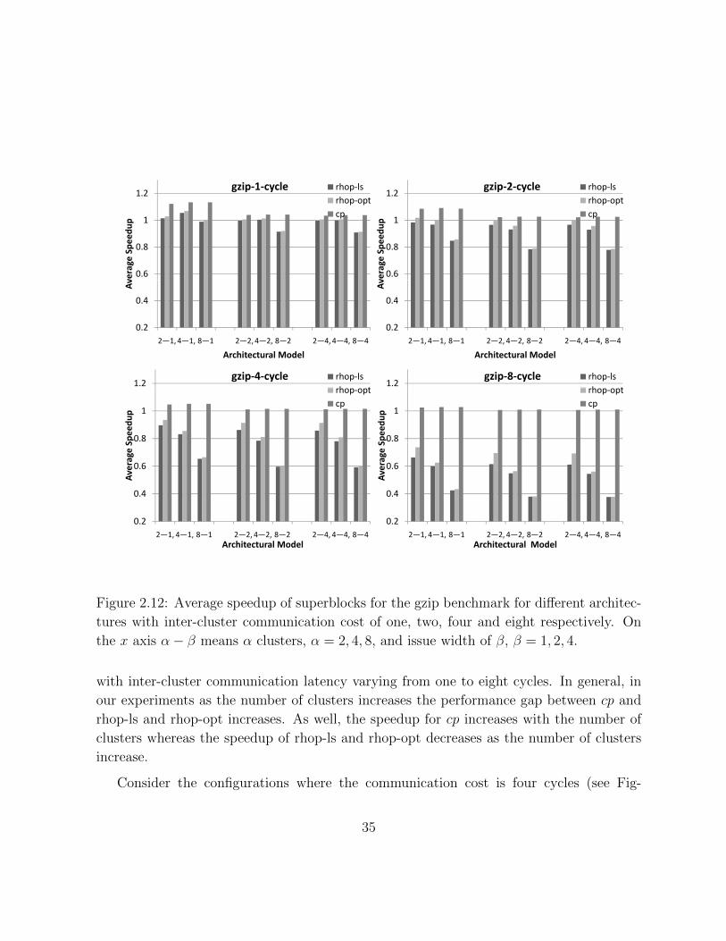
1

1.2

up

gzip‐2‐cycle rhop‐lsrhop‐optcp

1

1.2

up

gzip‐1‐cycle rhop‐lsrhop‐optcp

0.6

0.8

verage Spe

edu

0.6

0.8

verage Spe

edu

0.2

0.4

Av

0.2

0.4

Av

2―1, 4―1, 8―1 2―2, 4―2, 8―2 2―4, 4―4, 8―4

Architectural Model

1.2gzip‐4‐cycle rhop‐ls

rhop opt1.2

gzip‐8‐cycle rhop‐lsrhop opt

2―1,4―1, 8―1 2―2, 4―2, 8―2 2―4,4―4, 8―4

Architectural Model

0.8

1

Speedu

p

rhop‐optcp

0.8

1

Speedu

prhop‐optcp

0.4

0.6

Average S

0.4

0.6

Average S

0.22―1, 4―1, 8―1 2―2, 4―2, 8―2 2―4, 4―4, 8―4

Architectural Model

0.22―1, 4―1, 8―1 2―2, 4―2, 8―2 2―4, 4―4, 8―4

Architectural  Model

Figure 2.12: Average speedup of superblocks for the gzip benchmark for different architec-

tures with inter-cluster communication cost of one, two, four and eight respectively. On

the x axis α− β means α clusters, α = 2, 4, 8, and issue width of β, β = 1, 2, 4.

with inter-cluster communication latency varying from one to eight cycles. In general, in

our experiments as the number of clusters increases the performance gap between cp and

rhop-ls and rhop-opt increases. As well, the speedup for cp increases with the number of

clusters whereas the speedup of rhop-ls and rhop-opt decreases as the number of clusters

increase.

Consider the configurations where the communication cost is four cycles (see Fig-

35

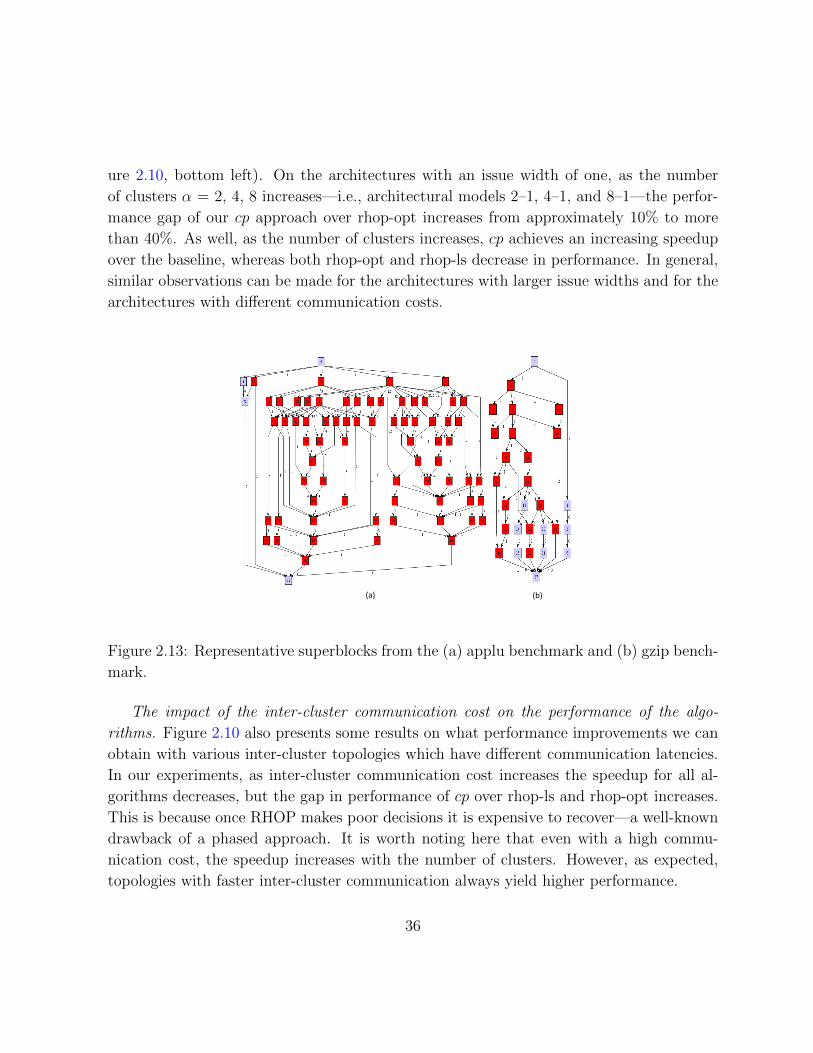
ure 2.10, bottom left). On the architectures with an issue width of one, as the number

of clusters α = 2, 4, 8 increases—i.e., architectural models 2–1, 4–1, and 8–1—the perfor-

mance gap of our cp approach over rhop-opt increases from approximately 10% to more

than 40%. As well, as the number of clusters increases, cp achieves an increasing speedup

over the baseline, whereas both rhop-opt and rhop-ls decrease in performance. In general,

similar observations can be made for the architectures with larger issue widths and for the

architectures with different communication costs.

(a) (b)

Figure 2.13: Representative superblocks from the (a) applu benchmark and (b) gzip bench-

mark.

The impact of the inter-cluster communication cost on the performance of the algo-

rithms. Figure 2.10 also presents some results on what performance improvements we can

obtain with various inter-cluster topologies which have different communication latencies.

In our experiments, as inter-cluster communication cost increases the speedup for all al-

gorithms decreases, but the gap in performance of cp over rhop-ls and rhop-opt increases.

This is because once RHOP makes poor decisions it is expensive to recover—a well-known

drawback of a phased approach. It is worth noting here that even with a high commu-

nication cost, the speedup increases with the number of clusters. However, as expected,

topologies with faster inter-cluster communication always yield higher performance.

36

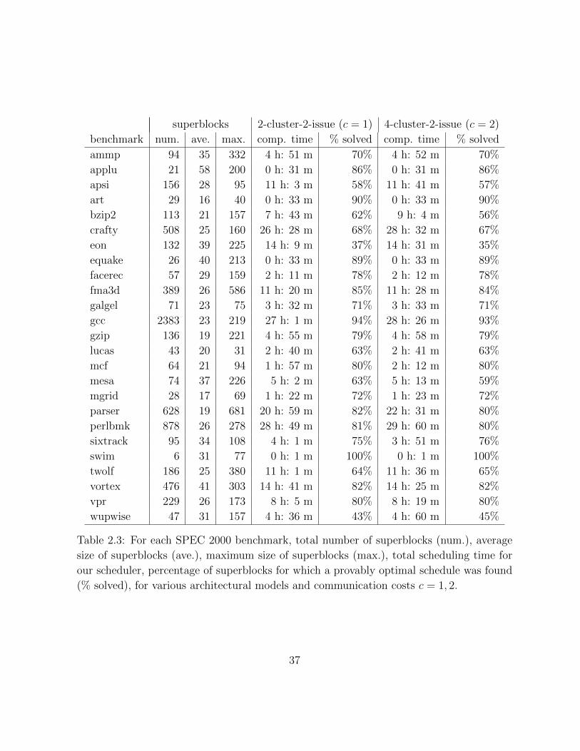
superblocks 2-cluster-2-issue (c = 1) 4-cluster-2-issue (c = 2)

benchmark num. ave. max. comp. time % solved comp. time % solved

ammp 94 35 332 4 h: 51 m 70% 4 h: 52 m 70%

applu 21 58 200 0 h: 31 m 86% 0 h: 31 m 86%

apsi 156 28 95 11 h: 3 m 58% 11 h: 41 m 57%

art 29 16 40 0 h: 33 m 90% 0 h: 33 m 90%

bzip2 113 21 157 7 h: 43 m 62% 9 h: 4 m 56%

crafty 508 25 160 26 h: 28 m 68% 28 h: 32 m 67%

eon 132 39 225 14 h: 9 m 37% 14 h: 31 m 35%

equake 26 40 213 0 h: 33 m 89% 0 h: 33 m 89%

facerec 57 29 159 2 h: 11 m 78% 2 h: 12 m 78%

fma3d 389 26 586 11 h: 20 m 85% 11 h: 28 m 84%

galgel 71 23 75 3 h: 32 m 71% 3 h: 33 m 71%

gcc 2383 23 219 27 h: 1 m 94% 28 h: 26 m 93%

gzip 136 19 221 4 h: 55 m 79% 4 h: 58 m 79%

lucas 43 20 31 2 h: 40 m 63% 2 h: 41 m 63%

mcf 64 21 94 1 h: 57 m 80% 2 h: 12 m 80%

mesa 74 37 226 5 h: 2 m 63% 5 h: 13 m 59%

mgrid 28 17 69 1 h: 22 m 72% 1 h: 23 m 72%

parser 628 19 681 20 h: 59 m 82% 22 h: 31 m 80%

perlbmk 878 26 278 28 h: 49 m 81% 29 h: 60 m 80%

sixtrack 95 34 108 4 h: 1 m 75% 3 h: 51 m 76%

swim 6 31 77 0 h: 1 m 100% 0 h: 1 m 100%

twolf 186 25 380 11 h: 1 m 64% 11 h: 36 m 65%

vortex 476 41 303 14 h: 41 m 82% 14 h: 25 m 82%

vpr 229 26 173 8 h: 5 m 80% 8 h: 19 m 80%

wupwise 47 31 157 4 h: 36 m 43% 4 h: 60 m 45%

Table 2.3: For each SPEC 2000 benchmark, total number of superblocks (num.), average

size of superblocks (ave.), maximum size of superblocks (max.), total scheduling time for

our scheduler, percentage of superblocks for which a provably optimal schedule was found

(% solved), for various architectural models and communication costs c = 1, 2.

37

Consider the configurations with four clusters and an issue width of one (see Fig-

ure 2.10). As expected, as the communication cost increases the performance of all of the

schedulers cp, rhop-opt, and rhop-ls decreases. More surprisingly, as the communication

cost c increases, the gap between the performance of cp and rhop-opt increases from 20%

when c = 1 to more than 35% when c = 8 (see architectural model 4–1 in Figure 2.10, for

c = 1 top left, c = 2 top right, c = 4 bottom left, and c = 8 bottom right). In general,

similar observations can be made for the architectures with larger issue widths and for the

architectures with different numbers of clusters.

Figures 2.11 and 2.12 present the breakdown of performance improvements for two spe-

cific benchmarks—applu and gzip, respectively—for various architectural configurations.

The applu benchmark (a floating point benchmark) is an example for which cp gets the

best speedup that approach a factor of 2.8 on an eight cluster architecture. Conversely, the

gzip benchmark (an integer benchmark) is an example where the speedup is more modest

and approach 15% on an eight cluster architecture, which is due to the lack of instruction-

level parallelism (ILP) in most SPEC integer benchmarks. For example, Figure 2.13 shows

two representative superblocks from the applu and gzip benchmarks, respectively. Of note

is the width of these graphs; i.e., there is much more available instruction level parallelism

in applu than in gzip.

The scheduling time and percentage of provably optimal schedules. Table 2.3 lists the

time it takes for the benchmarks to compile on two architectural configurations along with

the percentage of superblocks on which our algorithm proved optimality within the ten

minute timeout. The good news is that for almost all benchmarks cp can solve a majority

of the superblocks in the SPEC benchmarks to optimality. However this comes at a cost of

increased compilation time with some benchmarks requiring more than a day to schedule

all the superblocks in the benchmark. It is worth noting that even in the case where most

of the schedules are not provably optimal, we still get a speedup. In such cases we may well

have an optimal schedule but not provably so because the search algorithm timed out. For

example, for the benchmark eon (see Table 2.3), only 37% of the superblocks are solved

optimally yet cp yields a speedup of 15% on eon (see Figure 2.8). The scheduling times for

RHOP alone are not given as they are negligible and the scheduling times for RHOP-opt

are similar to the scheduling times for the optimal temporal scheduler alone (see [Malik et

al., 2008]).

38

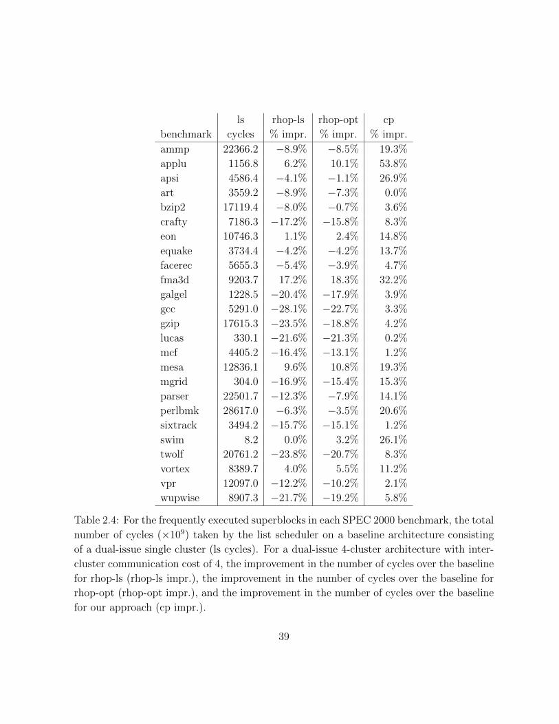
ls rhop-ls rhop-opt cp

benchmark cycles % impr. % impr. % impr.

ammp 22366.2 −8.9% −8.5% 19.3%

applu 1156.8 6.2% 10.1% 53.8%

apsi 4586.4 −4.1% −1.1% 26.9%

art 3559.2 −8.9% −7.3% 0.0%

bzip2 17119.4 −8.0% −0.7% 3.6%

crafty 7186.3 −17.2% −15.8% 8.3%

eon 10746.3 1.1% 2.4% 14.8%

equake 3734.4 −4.2% −4.2% 13.7%

facerec 5655.3 −5.4% −3.9% 4.7%

fma3d 9203.7 17.2% 18.3% 32.2%

galgel 1228.5 −20.4% −17.9% 3.9%

gcc 5291.0 −28.1% −22.7% 3.3%

gzip 17615.3 −23.5% −18.8% 4.2%

lucas 330.1 −21.6% −21.3% 0.2%

mcf 4405.2 −16.4% −13.1% 1.2%

mesa 12836.1 9.6% 10.8% 19.3%

mgrid 304.0 −16.9% −15.4% 15.3%

parser 22501.7 −12.3% −7.9% 14.1%

perlbmk 28617.0 −6.3% −3.5% 20.6%

sixtrack 3494.2 −15.7% −15.1% 1.2%

swim 8.2 0.0% 3.2% 26.1%

twolf 20761.2 −23.8% −20.7% 8.3%

vortex 8389.7 4.0% 5.5% 11.2%

vpr 12097.0 −12.2% −10.2% 2.1%

wupwise 8907.3 −21.7% −19.2% 5.8%

Table 2.4: For the frequently executed superblocks in each SPEC 2000 benchmark, the total

number of cycles (×109) taken by the list scheduler on a baseline architecture consisting

of a dual-issue single cluster (ls cycles). For a dual-issue 4-cluster architecture with inter-

cluster communication cost of 4, the improvement in the number of cycles over the baseline

for rhop-ls (rhop-ls impr.), the improvement in the number of cycles over the baseline for

rhop-opt (rhop-opt impr.), and the improvement in the number of cycles over the baseline

for our approach (cp impr.).

39

The weighted scheduling time and percentage improvement. Table 2.4 shows the fre-

quency based scheduling results for the frequently executed superblocks. A percentage

improvement is determined as follows. Each superblock in a benchmark is scheduled by

the given algorithm and the expected number of cycles for that superblock is computed

by multiplying the weighted completion time by the frequency of execution (as determined

by profiling). The total number of cycles is the sum of the expected number of cycles over

all superblocks. We then determine the percentage improvement over the baseline. For

example, for the benchmark ammp, rhop-ls achieves a percentage improvement of −8.9%

(i.e., it degrades performance by 8.9%), rhop-opt achieves a percentage improvement of

−8.5%, and cp achieves a percentage improvement of 19.3% (i.e., it improves performance

by 19.3%).

Overall, our experimental results show that our constraint programming approach pro-

duces better results than RHOP, as the number of clusters increases and also as the inter-

cluster latency increases. RHOP sometimes partitions the superblocks more aggressively

than necessary which results in a slowdown instead of a speedup, whereas our approach

always results in a speedup. The application of constraint programming to the spatial

scheduling problem has enabled us to solve the problem to near optimality for a significant

number of code blocks. Solving the spatial scheduling problem with constraint program-

ming has an added value over heuristic approaches in instances where longer compilation

time is tolerable or the code-base is not very large. This approach can be successfully

used in practice for software libraries, digital signal processing in addition to embedded

applications—domains where longer compile times are tolerable and the code is frequently

executed. Our approach can also be used to evaluate the performance of heuristic tech-

niques.

2.5 Related Work

Traditionally, instruction scheduling has been employed by compilers to exploit instruction

level parallelism in straight-line code in the form of basic blocks [Heffernan and Wilken,

2005; Malik et al., 2008] and superblocks [Heffernan et al., 2006; Malik et al., 2008]. In this

section we review the different approaches towards solving the spatial scheduling problem.

The most well known solutions for spatial scheduling are greedy and hierarchical par-

titioning algorithms which assign the instructions before the scheduling phase in the com-

40

piler. The bottom-up greedy, or BUG algorithm [Ellis, 1986], which is the earliest among

spatial scheduling algorithms, proceeds by recursing depth first along the data dependence

graph, assigning the critical paths first. It assigns each instruction to a cluster based on es-

timates of when the instruction and its predecessors can complete execution at the earliest.

These values are computed using the resource requirement information for each instruction.

The algorithm queries this information before and after the assignment to effectively assign

instructions to the available clusters. This technique works well for simple graphs, but as

the graphs become more complex the greedy nature of the algorithm directs it to make

decisions that negatively affect future decisions. Chung et al. [1995] also gave an early so-

lution to spatial scheduling for distributed memory multiprocessors based on heuristics for

list scheduling algorithms. Leupers [2000] present a combined partitioning and scheduling

technique using simulated annealing. Lapinskii et al. [2002] propose a binding algorithm

for instructions which relies on list scheduling to carry out temporal scheduling.

Lee et al. [2002] present a multi-heuristic framework for scheduling basic blocks, su-

perblocks and traces. The technique is called convergent scheduling. The scheduler main-

tains a three dimensional weight matrix Wi,c,t, where the ith dimension represents the

instructions, c spans over the number of clusters and t spans over possible time slots. The

scheduler iteratively executes multiple scheduling phases, each one of which heuristically

modifies the matrix to schedule each instruction on a cluster for a specific time slot, ac-

cording to a specific constraint. The main constraints are pre-placement, communication

minimization and load balancing. After several passes the weights are expected to converge.

The resultant matrix is used by a traditional scheduler to assign instructions to clusters.

The framework has been implemented on two different spatial architectures, RAW and

Chorus clustered VLIW infrastructure. The framework was evaluated on standard bench-

marks, mostly the ones with dense matrix code. An earlier attempt was made by the same

group for scheduling basic blocks in the Raw compiler [Lee et al., 1998]. Inter-cluster moves

on RAW take 3 or more cycles and the Chorus infrastructure assumes single cycle moves

in its simulation. This technique iteratively grouped together instructions with little or no

parallelism and then assigned them to the available clusters. A similar approach was used

to schedule instructions on a decoupled access/execute architectures [Rich and Farrens,

2000]. These techniques seem to work well on selective benchmark suites with fine tuned

system parameters which are configured using trial and error. It is difficult to evaluate the

actual effectiveness of these techniques mainly because they attempt to solve the temporal

and spatial scheduling intermittently. In contrast our approach attempts to solve spatial

41

scheduling first. In an earlier attempt on spatial scheduling [Amarasinghe et al., 2002]

presented integer linear formulations of the problem as well as an 8-approximation algo-

rithm for it. The evaluation in the unpublished report only included results from heuristic

algorithms and were from a simulation over a select group of benchmarks.

Chu et al. [2003] describe a region-based hierarchical operation partitioning algorithm

(RHOP), which is a pre-scheduling method to partition operations on multiple clusters. In

order to produce a partition that can result in an efficient schedule, RHOP uses schedule

estimates and a multilevel graph partitioner to generate cluster assignments. This approach

partitions a data dependence graph based on weighted vertices and edges. The algorithm

uses a heuristic to assign weights to the vertices to reflect their resource usage and to the

edges to reflect the cost of inter-cluster communication in case the two vertices connected

by an edge are assigned to different clusters. In the partitioning phase, vertices are grouped

together by two processes called coarsening and refinement [Hendrickson and Leland, 1995;

Karypis and Kumar, 1998]. Coarsening uses edge weights to group together operations by

iteratively pairing them into larger groups while targeting heavy edges first. The coarsening

phase ends when the number of groups is equal to the number of desired clusters for the

machine. The refinement phase improves the partition produced by the coarsening phase

by moving vertices from one partition to another. The goal of this phase is to improve the

balance between partitions while minimizing the overall communication cost. The moves

are considered feasible if there is an improvement in the gain from added parallelism minus

the cost of additional inter-cluster communications. The algorithm has been implemented

in the Trimaran compiler and simulation framework. The framework has the capability

to model homogeneous as well as heterogeneous architectures and assumes a single cycle

cost for inter-cluster moves. Their technique was evaluated on the SPEC benchmark and

compared against BUG, which RHOP always outperforms. Subsequent work using RHOP

partitions data over multi-core architectures with a more complex memory hierarchy [Chu

et al., 2007; Chu and Mahlke, 2006]. Unlike other approaches which are mostly evaluated

on basic blocks, RHOP has also been evaluated over hyperblocks.

Nagpal and Srikant [2004, 2008] give an integrated approach to spatial and tempo-

ral scheduling by binding the instructions to functional units in clusters. The approach

extends the list scheduling algorithm to incorporate a resource need vector for effective

functional unit binding. Their scheme utilizes the exact information about the available

communication requirements, functional units and the load on different clusters in addition

to the constraints imposed by the architecture to prioritize instructions that are ready to

42

be scheduled. The algorithm and its variations have been implemented for Texas Instru-

ments VelociTI architecture using the SUIF compiler framework. They evaluated their

technique using the TI simulator for TMS320C6X on the most frequently executed bench-

mark kernels from MediaBench and report a speedup of up to 19% over Lapinskii et al.

[2002].

In contrast to our work, which presents an optimal integrated approach for spatial

and temporal scheduling, Kessler, Bednarski, and Eriksson [Bednarski and Kessler, 2006;

Kessler and Bednarski, 2006; Eriksson and Kessler, 2009] pursue a much more ambitious

agenda of integrating spatial and temporal scheduling with instruction selection, register

allocation, and software pipelining. Although successful on smaller basic blocks, their fully

integrated approaches, which use dynamic programming and integer linear programming,

do not scale beyond blocks of size 20–40 instructions using a timeout of one hour (our

constraint programming technique scales consistently to blocks with up to 100 instructions

using a timeout of 10 minutes).

Other related works have also dealt with software pipelining for clustered architectures

[Nystrom and Eichenberger, 1998; Sanchez and Gonzalez, 2000; Codina et al., 2001]. Most

of these techniques extend the greedy scheduling algorithms and apply them after unrolling

frequently executed loops.

2.6 Summary

This chapter presents a constraint programming approach for spatial and temporal schedul-

ing problem for taking advantage of instruction level parallelism in clustered architectures.

We also study the effect of different hardware parameters including issue-width and cost

of inter-cluster communication performance.

Our approach takes advantage of the problem decomposition technique to solve spatial

scheduling in two stages, yet it is integrated with temporal scheduling. We also employ

various constraint programming techniques including symmetry breaking and branch-and-

bound to reduce the time in searching for a solution. Reformulation of the problem model in

terms of the edges of the DAG instead of the vertices breaks the symmetry nicely to reduce

the search space. In addition we also use techniques from graph theory to predetermine

instructions which can be grouped together before the search algorithm starts.

43

We compared our implementation against RHOP on various architectural configura-

tions. We found that our approach was able to achieve an improvement of up to 26%, on

average, over the state-of-the-art techniques on superblocks from SPEC 2000 benchmarks.

Clustered architectures are becoming increasingly important because they are a natural

way to extend the embedded processors without significant increase in power utilization,

which is vital for these architectures. Also many of the applications which run on em-

bedded devices are compiled once and usually run throughout the lifetime of the device

without recompilation and hence reasonably long compile times are also acceptable.

44

Chapter 3

Exact Instruction Selection

In this chapter we study the problem of instruction selection. Instruction selection is an

important phase in code generation that transforms the intermediate representation of code

to architecture specific machine instructions. It is a well studied problem and polynomial

time exact solutions have been proposed for instances where the intermediate representa-

tion is in the form of a tree. However, in most production compilers, intermediate code is

represented by directed acyclic graphs. Instruction selection is known to be NP-complete

on directed acyclic graphs. Production compilers employ graph heuristics incorporated into

dynamic programming algorithms to solve the problem approximately. In this chapter we

use constraint programming to model and solve the instruction selection problem. Previous

attempts at solving the problem optimally have not been general purpose or scale only to

basic blocks of size 40. Our constraint programming approach can solve basic blocks of size

100. We evaluate the constraint programming technique with two LLVM implementations

of carefully hand-tuned instruction selection algorithms. The results suggest that even

though the current state-of-the-art techniques have left little room for improvement, our

technique can be used to evaluate the accuracy of selection in different compilers.

3.1 Motivation

Advances in semiconductor technology and the pervasive use of consumer electronics have

fueled the advancement of general purpose computing as well as application specific devices

45

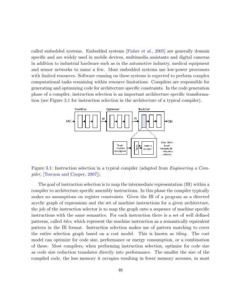
called embedded systems. Embedded systems [Fisher et al., 2005] are generally domain

specific and are widely used in mobile devices, multimedia assistants and digital cameras

in addition to industrial hardware such as in the automotive industry, medical equipment

and sensor networks to name a few. Most embedded systems use low-power processors

with limited resources. Software running on these systems is expected to perform complex

computational tasks remaining within resource limitations. Compilers are responsible for

generating and optimizing code for architecture specific constraints. In the code generation

phase of a compiler, instruction selection is an important architecture specific transforma-

tion (see Figure 3.1 for instruction selection in the architecture of a typical compiler).

Figure 3.1: Instruction selection in a typical compiler (adapted from Engineering a Com-

piler, [Torczon and Cooper, 2007]).

The goal of instruction selection is to map the intermediate representation (IR) within a

compiler to architecture specific assembly instructions. In this phase the compiler typically

makes no assumptions on register constraints. Given the IR of a program as a directed

acyclic graph of expressions and the set of machine instructions for a given architecture,

the job of the instruction selector is to map the graph onto a sequence of machine specific

instructions with the same semantics. For each instruction there is a set of well defined

patterns, called tiles, which represent the machine instruction as a semantically equivalent

pattern in the IR format. Instruction selection makes use of pattern matching to cover

the entire selection graph based on a cost model. This is known as tiling. The cost

model can optimize for code size, performance or energy consumption, or a combination

of these. Most compilers, when performing instruction selection, optimize for code size

as code size reduction translates directly into performance. The smaller the size of the

compiled code, the less memory it occupies resulting in fewer memory accesses, in most

46

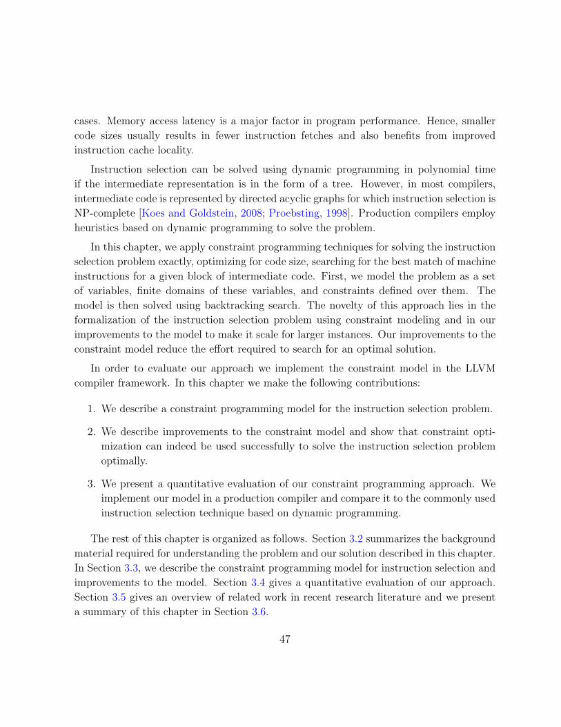
cases. Memory access latency is a major factor in program performance. Hence, smaller

code sizes usually results in fewer instruction fetches and also benefits from improved

instruction cache locality.

Instruction selection can be solved using dynamic programming in polynomial time

if the intermediate representation is in the form of a tree. However, in most compilers,

intermediate code is represented by directed acyclic graphs for which instruction selection is

NP-complete [Koes and Goldstein, 2008; Proebsting, 1998]. Production compilers employ

heuristics based on dynamic programming to solve the problem.

In this chapter, we apply constraint programming techniques for solving the instruction

selection problem exactly, optimizing for code size, searching for the best match of machine

instructions for a given block of intermediate code. First, we model the problem as a set

of variables, finite domains of these variables, and constraints defined over them. The

model is then solved using backtracking search. The novelty of this approach lies in the

formalization of the instruction selection problem using constraint modeling and in our

improvements to the model to make it scale for larger instances. Our improvements to the

constraint model reduce the effort required to search for an optimal solution.

In order to evaluate our approach we implement the constraint model in the LLVM

compiler framework. In this chapter we make the following contributions:

1. We describe a constraint programming model for the instruction selection problem.

2. We describe improvements to the constraint model and show that constraint opti-

mization can indeed be used successfully to solve the instruction selection problem

optimally.

3. We present a quantitative evaluation of our constraint programming approach. We

implement our model in a production compiler and compare it to the commonly used

instruction selection technique based on dynamic programming.

The rest of this chapter is organized as follows. Section 3.2 summarizes the background

material required for understanding the problem and our solution described in this chapter.

In Section 3.3, we describe the constraint programming model for instruction selection and

improvements to the model. Section 3.4 gives a quantitative evaluation of our approach.

Section 3.5 gives an overview of related work in recent research literature and we present

a summary of this chapter in Section 3.6.

47

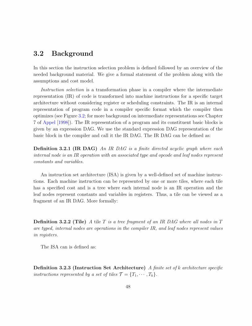
3.2 Background

In this section the instruction selection problem is defined followed by an overview of the

needed background material. We give a formal statement of the problem along with the

assumptions and cost model.

Instruction selection is a transformation phase in a compiler where the intermediate

representation (IR) of code is transformed into machine instructions for a specific target

architecture without considering register or scheduling constraints. The IR is an internal

representation of program code in a compiler specific format which the compiler then

optimizes (see Figure 3.2; for more background on intermediate representations see Chapter

7 of Appel [1998]). The IR representation of a program and its constituent basic blocks is

given by an expression DAG. We use the standard expression DAG representation of the

basic block in the compiler and call it the IR DAG. The IR DAG can be defined as:

Definition 3.2.1 (IR DAG) An IR DAG is a finite directed acyclic graph where each

internal node is an IR operation with an associated type and opcode and leaf nodes represent

constants and variables.

An instruction set architecture (ISA) is given by a well-defined set of machine instruc-

tions. Each machine instruction can be represented by one or more tiles, where each tile

has a specified cost and is a tree where each internal node is an IR operation and the

leaf nodes represent constants and variables in registers. Thus, a tile can be viewed as a

fragment of an IR DAG. More formally:

Definition 3.2.2 (Tile) A tile T is a tree fragment of an IR DAG where all nodes in T

are typed, internal nodes are operations in the compiler IR, and leaf nodes represent values

in registers.

The ISA can is defined as:

Definition 3.2.3 (Instruction Set Architecture) A finite set of k architecture specific

instructions represented by a set of tiles T = {T1, · · · , Tk}.

48

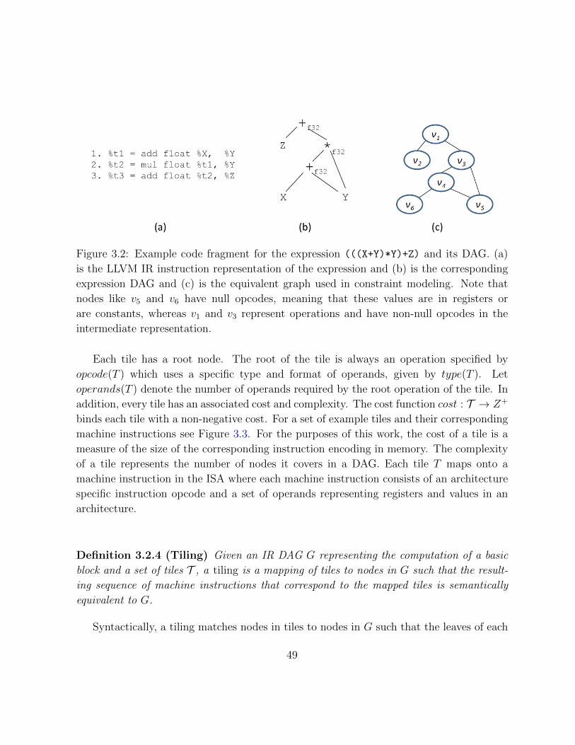
Figure 3.2: Example code fragment for the expression (((X+Y)*Y)+Z) and its DAG. (a)

is the LLVM IR instruction representation of the expression and (b) is the corresponding

expression DAG and (c) is the equivalent graph used in constraint modeling. Note that

nodes like v5 and v6 have null opcodes, meaning that these values are in registers or

are constants, whereas v1 and v3 represent operations and have non-null opcodes in the

intermediate representation.

Each tile has a root node. The root of the tile is always an operation specified by

opcode(T ) which uses a specific type and format of operands, given by type(T ). Let

operands(T ) denote the number of operands required by the root operation of the tile. In

addition, every tile has an associated cost and complexity. The cost function cost : T → Z+

binds each tile with a non-negative cost. For a set of example tiles and their corresponding

machine instructions see Figure 3.3. For the purposes of this work, the cost of a tile is a

measure of the size of the corresponding instruction encoding in memory. The complexity

of a tile represents the number of nodes it covers in a DAG. Each tile T maps onto a

machine instruction in the ISA where each machine instruction consists of an architecture

specific instruction opcode and a set of operands representing registers and values in an

architecture.

Definition 3.2.4 (Tiling) Given an IR DAG G representing the computation of a basic

block and a set of tiles T , a tiling is a mapping of tiles to nodes in G such that the result-

ing sequence of machine instructions that correspond to the mapped tiles is semantically

equivalent to G.

Syntactically, a tiling matches nodes in tiles to nodes in G such that the leaves of each

49

Figure 3.3: A subset of relevant tiles for a PowerPC architecture and the corresponding

instructions. The first instruction adds the two values in the given floating point registers

($FRA and $FRB), whereas the second multiplies the two register values. The result is

stored in the target register ($FRT). The third instruction multiplies its first two operand

and adds the result to the third. The register values are marked with an r with the

subscript showing that it is of floating point type.

tile are either available as the roots of other tiles or they are available as register values,

and each operation node in G is uniquely mapped to an internal node of a tile. For a tile

to match, two constraints must hold. First, the type constraints enforce that the type of

each tile node must be the same as the type of the corresponding node in G. Second, the

structural constraints enforce that the number of successors of each tile node must be the

same as the number of successors of the corresponding node in G. Additionally, a tiling

must satisfy a coverage constraint that enforces that every node in G is covered; i.e., there

are no nodes in G that are not mapped by some tile. For an example of tiling see Figure

3.4.

Example 3.2.5 Consider the example given in Figure 3.2 which shows an IR DAG for

the given intermediate code. Given a set of tiles for a specific architecture given in Figure

3.3, the IR DAG can be tiled in different ways as shown in Figure 3.4. The better tiling

(b) requires only two tiles with a cost of 8 whereas the alternate tiling requires three tiles

with a cost of 9.

The optimal tiling of an IR DAG is the tiling with the smallest cost. The goal of this

work is to generate a tiling such that the tiling cost is minimized. The instruction selection

problem can be defined formally as:

50

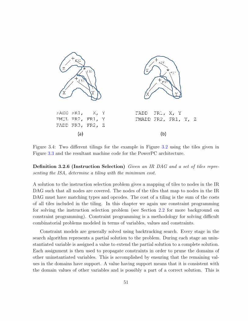
Figure 3.4: Two different tilings for the example in Figure 3.2 using the tiles given in

Figure 3.3 and the resultant machine code for the PowerPC architecture.

Definition 3.2.6 (Instruction Selection) Given an IR DAG and a set of tiles repre-

senting the ISA, determine a tiling with the minimum cost.

A solution to the instruction selection problem gives a mapping of tiles to nodes in the IR

DAG such that all nodes are covered. The nodes of the tiles that map to nodes in the IR

DAG must have matching types and opcodes. The cost of a tiling is the sum of the costs

of all tiles included in the tiling. In this chapter we again use constraint programming

for solving the instruction selection problem (see Section 2.2 for more background on

constraint programming). Constraint programming is a methodology for solving difficult

combinatorial problems modeled in terms of variables, values and constraints.

Constraint models are generally solved using backtracking search. Every stage in the

search algorithm represents a partial solution to the problem. During each stage an unin-

stantiated variable is assigned a value to extend the partial solution to a complete solution.

Each assignment is then used to propagate constraints in order to prune the domains of

other uninstantiated variables. This is accomplished by ensuring that the remaining val-

ues in the domains have support. A value having support means that it is consistent with

the domain values of other variables and is possibly a part of a correct solution. This is

51

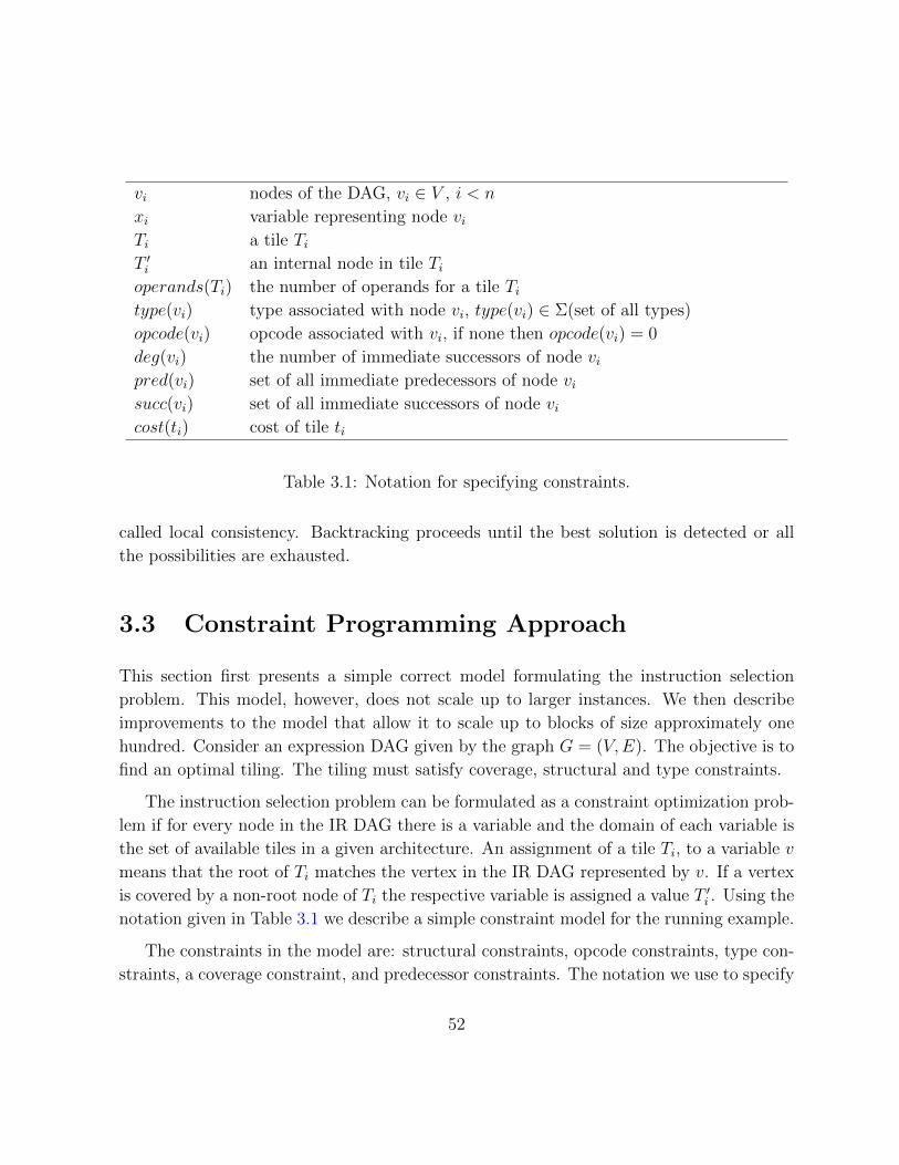
vi nodes of the DAG, vi ∈ V , i < n

xi variable representing node viTi a tile TiT ′i an internal node in tile Tioperands(Ti) the number of operands for a tile Titype(vi) type associated with node vi, type(vi) ∈ Σ(set of all types)

opcode(vi) opcode associated with vi, if none then opcode(vi) = 0

deg(vi) the number of immediate successors of node vipred(vi) set of all immediate predecessors of node visucc(vi) set of all immediate successors of node vicost(ti) cost of tile ti

Table 3.1: Notation for specifying constraints.

called local consistency. Backtracking proceeds until the best solution is detected or all

the possibilities are exhausted.

3.3 Constraint Programming Approach

This section first presents a simple correct model formulating the instruction selection

problem. This model, however, does not scale up to larger instances. We then describe

improvements to the model that allow it to scale up to blocks of size approximately one

hundred. Consider an expression DAG given by the graph G = (V,E). The objective is to

find an optimal tiling. The tiling must satisfy coverage, structural and type constraints.

The instruction selection problem can be formulated as a constraint optimization prob-

lem if for every node in the IR DAG there is a variable and the domain of each variable is

the set of available tiles in a given architecture. An assignment of a tile Ti, to a variable v

means that the root of Ti matches the vertex in the IR DAG represented by v. If a vertex

is covered by a non-root node of Ti the respective variable is assigned a value T ′i . Using the

notation given in Table 3.1 we describe a simple constraint model for the running example.

The constraints in the model are: structural constraints, opcode constraints, type con-

straints, a coverage constraint, and predecessor constraints. The notation we use to specify

52

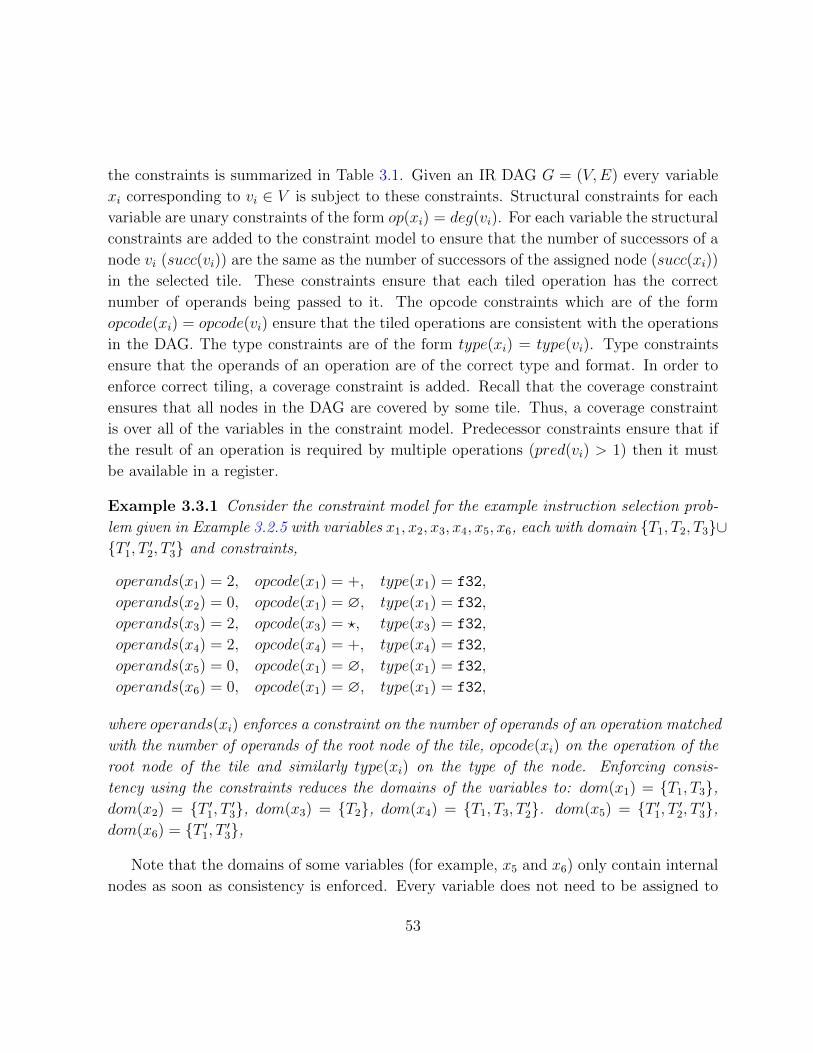
the constraints is summarized in Table 3.1. Given an IR DAG G = (V,E) every variable

xi corresponding to vi ∈ V is subject to these constraints. Structural constraints for each

variable are unary constraints of the form op(xi) = deg(vi). For each variable the structural

constraints are added to the constraint model to ensure that the number of successors of a

node vi (succ(vi)) are the same as the number of successors of the assigned node (succ(xi))

in the selected tile. These constraints ensure that each tiled operation has the correct

number of operands being passed to it. The opcode constraints which are of the form

opcode(xi) = opcode(vi) ensure that the tiled operations are consistent with the operations

in the DAG. The type constraints are of the form type(xi) = type(vi). Type constraints

ensure that the operands of an operation are of the correct type and format. In order to

enforce correct tiling, a coverage constraint is added. Recall that the coverage constraint

ensures that all nodes in the DAG are covered by some tile. Thus, a coverage constraint

is over all of the variables in the constraint model. Predecessor constraints ensure that if

the result of an operation is required by multiple operations (pred(vi) > 1) then it must

be available in a register.

Example 3.3.1 Consider the constraint model for the example instruction selection prob-

lem given in Example 3.2.5 with variables x1, x2, x3, x4, x5, x6, each with domain {T1, T2, T3}∪{T ′1, T ′2, T ′3} and constraints,

operands(x1) = 2, opcode(x1) = +, type(x1) = f32,

operands(x2) = 0, opcode(x1) = ∅, type(x1) = f32,

operands(x3) = 2, opcode(x3) = ?, type(x3) = f32,

operands(x4) = 2, opcode(x4) = +, type(x4) = f32,

operands(x5) = 0, opcode(x1) = ∅, type(x1) = f32,

operands(x6) = 0, opcode(x1) = ∅, type(x1) = f32,

where operands(xi) enforces a constraint on the number of operands of an operation matched

with the number of operands of the root node of the tile, opcode(xi) on the operation of the

root node of the tile and similarly type(xi) on the type of the node. Enforcing consis-

tency using the constraints reduces the domains of the variables to: dom(x1) = {T1, T3},dom(x2) = {T ′1, T ′3}, dom(x3) = {T2}, dom(x4) = {T1, T3, T ′2}. dom(x5) = {T ′1, T ′2, T ′3},dom(x6) = {T ′1, T ′3},

Note that the domains of some variables (for example, x5 and x6) only contain internal

nodes as soon as consistency is enforced. Every variable does not need to be assigned to

53

be the root of a tile. A solution is valid as long as all nodes in the IR DAG are covered by

some tile.

We model each node vi ∈ V , of the IR DAG with a variable xi. The domain of each

variable is dom(xi) = {T1, . . . , Tk} ∪ {T ′1, . . . , T ′k}, which is the set of available tiles in a

given target set architecture. Assigning a tile Ti to a variable xj has the intended meaning

that the node vj in the DAG will be covered by tile Ti.

What has been described above is the minimal correct model for the instruction selec-

tion problem. It is well known that adding implied constraints, symmetry breaking and

preprocessing techniques can greatly improve the efficiency of the search for a solution.

Without these improvements the search does not scale beyond DAGs of size 30 to 40.

With the improved model the search scales up to instances of size 100 to 200 and is able

to get the optimal solutions for a vast majority of benchmark blocks.

3.3.1 Selection Algorithm

Given an instance of the instruction selection problem, the solution proceeds in two phases.

The first phase consists of constructing a constraint model and some preprocessing to refine

the model by pruning the domains. The second phase consists of backtracking search with

constraint propagation.

A sketch of the selection algorithm is given as Algorithm 3. The first phase consists

of constructing the constraint model by setting up the variables, their domains as being

the set of all tiles, and constraints. It proceeds with domain preprocessing where the

domain of each variable is pruned as described earlier. An upper bound on selection cost

is established using a dynamic programming algorithm [Appel, 1998, p.197]. The tiling

from the dynamic programming algorithm which corresponds to the upper bound is used

as the seed tiling in the search and is used to prune the search. If the cost of a partial

tiling exceeds the cost of the current upper bound the search tree is pruned. The constraint

model and the upper bound are passed onto the backtracking algorithm.

The second phase consists of backtracking search over the refined model. Backtrack-

ing search interleaves constraint propagation along with branch and bound checks as it

branches over the variable assignments (see Algorithm 4). Once an unassigned variable

is selected (line 9), matching tiles are iteratively assigned to the selected variable if the

match is found to be consistent with the current partial tiling.

54

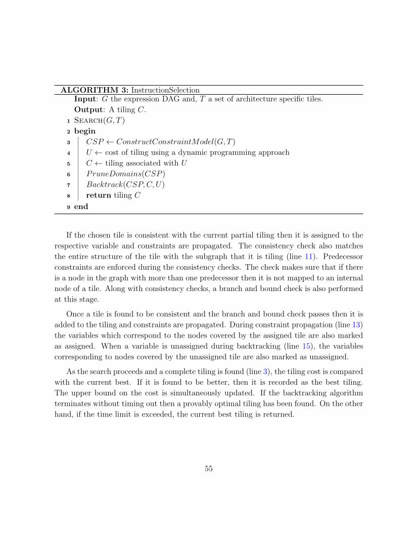
ALGORITHM 3: InstructionSelectionInput: G the expression DAG and, T a set of architecture specific tiles.

Output: A tiling C.

1 Search(G, T )

2 begin

3 CSP ← ConstructConstraintModel(G, T )

4 U ← cost of tiling using a dynamic programming approach

5 C ← tiling associated with U

6 PruneDomains(CSP )

7 Backtrack(CSP,C, U)

8 return tiling C

9 end

If the chosen tile is consistent with the current partial tiling then it is assigned to the

respective variable and constraints are propagated. The consistency check also matches

the entire structure of the tile with the subgraph that it is tiling (line 11). Predecessor

constraints are enforced during the consistency checks. The check makes sure that if there

is a node in the graph with more than one predecessor then it is not mapped to an internal

node of a tile. Along with consistency checks, a branch and bound check is also performed

at this stage.

Once a tile is found to be consistent and the branch and bound check passes then it is

added to the tiling and constraints are propagated. During constraint propagation (line 13)

the variables which correspond to the nodes covered by the assigned tile are also marked

as assigned. When a variable is unassigned during backtracking (line 15), the variables

corresponding to nodes covered by the unassigned tile are also marked as unassigned.

As the search proceeds and a complete tiling is found (line 3), the tiling cost is compared

with the current best. If it is found to be better, then it is recorded as the best tiling.

The upper bound on the cost is simultaneously updated. If the backtracking algorithm

terminates without timing out then a provably optimal tiling has been found. On the other

hand, if the time limit is exceeded, the current best tiling is returned.

55

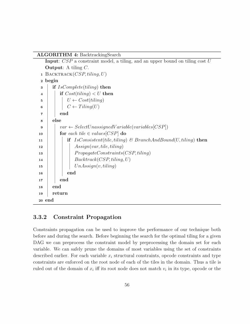
ALGORITHM 4: BacktrackingSearch

Input: CSP a constraint model, a tiling, and an upper bound on tiling cost U

Output: A tiling C.

1 Backtrack(CSP, tiling, U)

2 begin

3 if IsComplete(tiling) then

4 if Cost(tiling) < U then

5 U ← Cost(tiling)

6 C ← Tiling(U)

7 end

8 else

9 var ← SelectUnassignedV ariable(variables[CSP ])

10 for each tile ∈ values[CSP ] do

11 if IsConsistent(tile, tiling) & BranchAndBound(U, tiling) then

12 Assign(var, tile, tiling)

13 PropagateConstraints(CSP, tiling)

14 Backtrack(CSP, tiling, U)

15 UnAssign(v, tiling)

16 end

17 end

18 end

19 return

20 end

3.3.2 Constraint Propagation

Constraints propagation can be used to improve the performance of our technique both

before and during the search. Before beginning the search for the optimal tiling for a given

DAG we can preprocess the constraint model by preprocessing the domain set for each

variable. We can safely prune the domains of most variables using the set of constraints

described earlier. For each variable xi structural constraints, opcode constraints and type

constraints are enforced on the root node of each of the tiles in the domain. Thus a tile is

ruled out of the domain of xi iff its root node does not match vi in its type, opcode or the

56

number of successors. This significantly reduces the size of the domains for each variable.

Example 3.3.2 Consider Example 3.3.1 which describes the constraint model for our run-

ning example. Simply enforcing the three constraints reduces dom(x3) to {T2} and the

domains of x2, x5 and x6 to internal nodes of tiles only. In the case of x3, the only tile

among {T1, T2, T3} whose opcode at the root node (opcode(x3) = ?) matches the node v3’s

opcode is T2 and hence the other tiles are pruned from the domain of x3. A domain with

only internal nodes means that there are no tiles in the domain set which can be rooted at

that node. The coverage constraint ensures that all nodes in the DAG are covered.

After the preprocessing phase, the domain of each variable has been pruned to a subset

of tiles which can be rooted at the corresponding node in the DAG. Pruning only removes

domain values that cannot be part of a solution. Using the root of a tile for matching

ensures that if a node in the IR DAG can be matched to a node in a tile, that tile is in the

domain of the variable where it should be rooted if it is included in a tiling.

During the search, constraints are propagated as variables are assigned values. Once a

tile is assigned to a variable all the nodes in the DAG that match the tile nodes are marked

as covered and corresponding variables in the model are marked as assigned. This means

that these variables are not considered as the search progresses down the tree which results

in fewer branches on the path to the leaf nodes (i.e., solutions).

Constraint propagation also handles over-tiling. Over-tiling refers to operation nodes

being covered by multiple tiles. Over-tiling may not result in incorrect code, but can delay

the search for the optimal solution. The following example highlights how over-tiling is

handled by our approach.

Example 3.3.3 Consider the example given in Figure 3.5 which illustrates constraint

propagation during the tiling of the running example. If x3 is the first variable to be

assigned a value, i.e. T2, the partial tiling looks like Figure 3.5(a). Subsequently when x1is assigned the tile T3, the partial tiling looks like Figure 3.5(b) which means that v3 is

now over-tiled. This over-tiling may not result in incorrect code but the cost of this par-

tial tiling is eight. When the constraints are propagated, this over-tiling is detected as the

cost exceeds the current upper bound. Thus, the value of T2 is removed from the domain

of x3—as illustrated in Figure 3.5(c)—bringing down the cost of the partial tiling to five.

This partial tiling is part of the optimal solution in this case.

57

Figure 3.5: (a) Tile T2 assigned to variable x3 in the constraint model. (b) later in the

search tile T3 is assigned to variable x1 in the constraint model. (c) Propagating constraints

prunes the domain of x3 as it handles over-tiling.

Constraint propagation not only reduces the search space but also enforces consistency

of the tiling by propagating predecessor constraints. Predecessor constraints ensure that if

the result of an operation is required by more than one operation then its result is available

as a register value (see Figure 3.3). Recall that once an operation instruction is executed

its result is available in a register. During constraint propagation it is made sure that when

such nodes are tiled the operation is covered by the root of a tile. See Figure 3.6 for an

example.

3.3.3 Branch and Bound

Branch and bound refers to a check at each assignment during the backtracking algorithm

to recognize early in the search whether the solutions within the sub tree would be optimally

feasible or not. A fast dynamic programming solution for selecting instructions is used to

obtain a solution which is recorded as the best initial solution and its cost is recorded as

the upper bound on the cost of tiling. As the search progresses during backtracking the

upper bound is updated.

The update happens as we find better solutions during the search and the upper bound

reflects the cost of the best solution so far. The cost of each partial tiling is compared with

this upper bound at each internal node in the search tree. If the cost is found to be above

the upper bound the search does not descend the tree any further.

58

Figure 3.6: (a) Tile T3 is assigned to a variable in the constraint model. (b) Another

variable assigned tile to T1. Due to a predecessor constraint, this is inconsistent as one of

the operands of T1 is not available as a register value. (c) T2 would be the correct tile to

choose in this case.

3.4 Experimental Evaluation

In this section we present the performance results of our constraint programming approach

for the instruction selection problem. We describe the implementation framework, experi-

mental setup and a quantitative analysis of the results in the following subsections.

3.4.1 Implementation Framework

The constraint programming model has been implemented in the LLVM 3.0 [Lattner and

Avde, 2004] compiler infrastructure. We modified the common code selection algorithm to

incorporate our constraint programming approach. LLVM provides a hand-tuned dynamic

programming selection algorithm as well as a greedy selector based on BURG [Fraser

et al., 1992] (see the Related Work, Section 3.5 for a description of these approaches).

We compare the performance of our approach primarily with the default LLVM selection

algorithm which is an implementation of the dynamic programming solution. In addition

we compare the effect of all three approaches on code size.

59

3.4.2 Experimental Setup

We evaluated the constraint programming implementation on C and C++ benchmarks

from the MiBench [MiBench, 2001], MediaBench [MediaBench, 1997] and VersaBench

[VersaBench, 2004]. The benchmarks were compiled using the LLVM compiler frame-

work. The compilations were done at two different levels of optimizations, −Os which

aggressively optimizes for code size and −O3 which includes more complex optimization

techniques such as loop unrolling but may result in larger code. Some of the benchmarks

like ghostscript, mpeg2, pegwit, and pgp from MediaBench have been omitted because

LLVM fails to compile them completely with issues unrelated to instruction selection.

Our algorithm works on basic block expression DAGs also known as Selection DAGs in

LLVM. It is worth noting that instruction selection is practically the first phase in backend

compiler optimizations and precedes both instruction scheduling and register allocation.

3.4.3 Experimental Results & Analysis

In this section we present the results of our experiments. First, we compare the cost of

tiling of our constraint programming algorithm with the tiling cost of the better of the

two LLVM selection algorithms which is also the LLVM default: dynamic programming

selector (DP). Second, we compare the impact on code size for our optimal tiling approach

against the dynamic programming approach. Third, we examine the impact of the more

aggressive optimization level, −O3, on selection cost and code size. Finally, as our optimal

selector is more costly in terms of selection time, we examine the additional time taken to

perform instruction selection on the benchmarks. All of the results presented are for the

x86 architecture unless specified otherwise.

Improvements in selection cost and percentage of provably optimal tilings. Performance

results for our instruction selection algorithm are given in Table 3.2. Our algorithm is able

to solve more than 90% of the basic blocks within each benchmark optimally. However,

the average improvements in selection cost do not exceed 4% for any benchmark even with

the increased compilation time. For some smaller benchmarks there is no improvement at

all (for example, crc32 and qsort) even though all the blocks were solved optimally. This

is partly due to the small size and fewer basic blocks in the benchmark and partly due to

the highly optimized nature of dynamic programming selector of LLVM which does not

produce provably optimal solutions but appears to be close to optimal in practice.

60

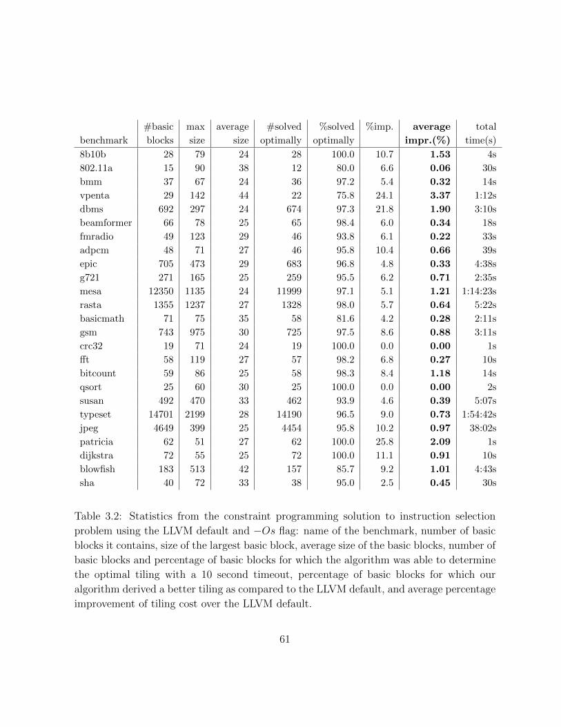
#basic max average #solved %solved %imp. average total

benchmark blocks size size optimally optimally impr.(%) time(s)

8b10b 28 79 24 28 100.0 10.7 1.53 4s

802.11a 15 90 38 12 80.0 6.6 0.06 30s

bmm 37 67 24 36 97.2 5.4 0.32 14s

vpenta 29 142 44 22 75.8 24.1 3.37 1:12s

dbms 692 297 24 674 97.3 21.8 1.90 3:10s

beamformer 66 78 25 65 98.4 6.0 0.34 18s

fmradio 49 123 29 46 93.8 6.1 0.22 33s

adpcm 48 71 27 46 95.8 10.4 0.66 39s

epic 705 473 29 683 96.8 4.8 0.33 4:38s

g721 271 165 25 259 95.5 6.2 0.71 2:35s

mesa 12350 1135 24 11999 97.1 5.1 1.21 1:14:23s

rasta 1355 1237 27 1328 98.0 5.7 0.64 5:22s

basicmath 71 75 35 58 81.6 4.2 0.28 2:11s

gsm 743 975 30 725 97.5 8.6 0.88 3:11s

crc32 19 71 24 19 100.0 0.0 0.00 1s

fft 58 119 27 57 98.2 6.8 0.27 10s

bitcount 59 86 25 58 98.3 8.4 1.18 14s

qsort 25 60 30 25 100.0 0.0 0.00 2s

susan 492 470 33 462 93.9 4.6 0.39 5:07s

typeset 14701 2199 28 14190 96.5 9.0 0.73 1:54:42s

jpeg 4649 399 25 4454 95.8 10.2 0.97 38:02s

patricia 62 51 27 62 100.0 25.8 2.09 1s

dijkstra 72 55 25 72 100.0 11.1 0.91 10s

blowfish 183 513 42 157 85.7 9.2 1.01 4:43s

sha 40 72 33 38 95.0 2.5 0.45 30s

Table 3.2: Statistics from the constraint programming solution to instruction selection

problem using the LLVM default and −Os flag: name of the benchmark, number of basic

blocks it contains, size of the largest basic block, average size of the basic blocks, number of

basic blocks and percentage of basic blocks for which the algorithm was able to determine

the optimal tiling with a 10 second timeout, percentage of basic blocks for which our

algorithm derived a better tiling as compared to the LLVM default, and average percentage

improvement of tiling cost over the LLVM default.

61

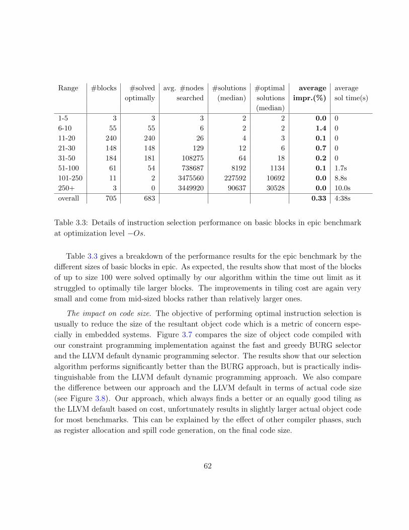
Range #blocks #solved avg. #nodes #solutions #optimal average average

optimally searched (median) solutions impr.(%) sol time(s)

(median)

1-5 3 3 3 2 2 0.0 0

6-10 55 55 6 2 2 1.4 0

11-20 240 240 26 4 3 0.1 0

21-30 148 148 129 12 6 0.7 0

31-50 184 181 108275 64 18 0.2 0

51-100 61 54 738687 8192 1134 0.1 1.7s

101-250 11 2 3475560 227592 10692 0.0 8.8s

250+ 3 0 3449920 90637 30528 0.0 10.0s

overall 705 683 0.33 4:38s

Table 3.3: Details of instruction selection performance on basic blocks in epic benchmark

at optimization level −Os.

Table 3.3 gives a breakdown of the performance results for the epic benchmark by the

different sizes of basic blocks in epic. As expected, the results show that most of the blocks

of up to size 100 were solved optimally by our algorithm within the time out limit as it

struggled to optimally tile larger blocks. The improvements in tiling cost are again very

small and come from mid-sized blocks rather than relatively larger ones.

The impact on code size. The objective of performing optimal instruction selection is

usually to reduce the size of the resultant object code which is a metric of concern espe-

cially in embedded systems. Figure 3.7 compares the size of object code compiled with

our constraint programming implementation against the fast and greedy BURG selector

and the LLVM default dynamic programming selector. The results show that our selection

algorithm performs significantly better than the BURG approach, but is practically indis-

tinguishable from the LLVM default dynamic programming approach. We also compare

the difference between our approach and the LLVM default in terms of actual code size

(see Figure 3.8). Our approach, which always finds a better or an equally good tiling as

the LLVM default based on cost, unfortunately results in slightly larger actual object code

for most benchmarks. This can be explained by the effect of other compiler phases, such

as register allocation and spill code generation, on the final code size.

62

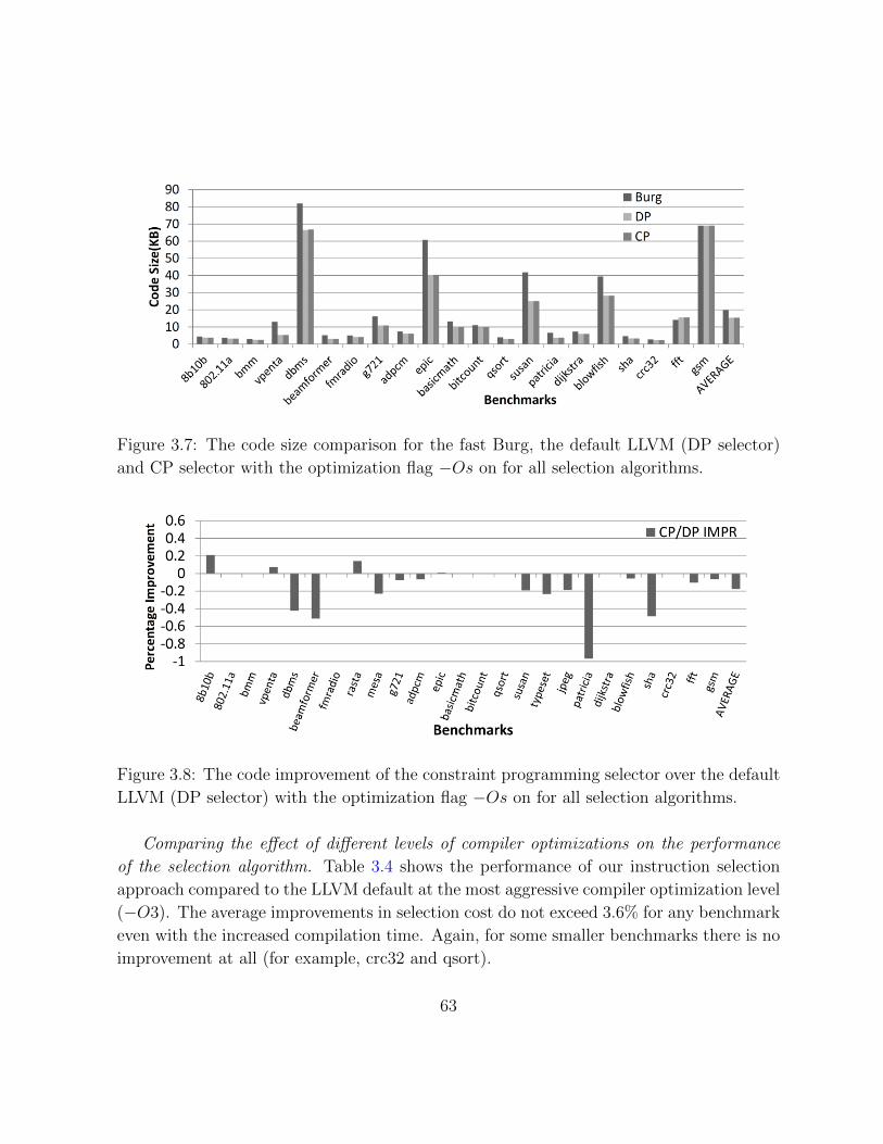
Figure 3.7: The code size comparison for the fast Burg, the default LLVM (DP selector)

and CP selector with the optimization flag −Os on for all selection algorithms.

Figure 3.8: The code improvement of the constraint programming selector over the default

LLVM (DP selector) with the optimization flag −Os on for all selection algorithms.

Comparing the effect of different levels of compiler optimizations on the performance

of the selection algorithm. Table 3.4 shows the performance of our instruction selection

approach compared to the LLVM default at the most aggressive compiler optimization level

(−O3). The average improvements in selection cost do not exceed 3.6% for any benchmark

even with the increased compilation time. Again, for some smaller benchmarks there is no

improvement at all (for example, crc32 and qsort).

63

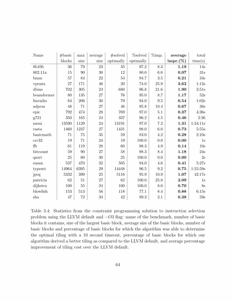
Name #basic max average #solved %solved %imp. average total

blocks size size optimally optimally impr.(%) time(s)

8b10b 36 79 23 35 97.2 8.3 1.19 14s

802.11a 15 90 38 12 80.0 6.6 0.07 31s

bmm 57 84 22 54 94.7 3.5 0.21 34s

vpenta 27 171 46 20 74.0 25.9 3.62 1:12s

dbms 702 305 24 680 96.8 21.6 1.90 3:51s

beamformer 80 135 27 76 95.0 8.7 1.17 52s

fmradio 84 206 30 79 94.0 9.5 0.54 1:02s

adpcm 48 71 27 46 95.8 10.4 0.67 38s

epic 792 474 28 769 97.0 5.1 0.37 4:36s

g721 350 165 24 337 96.2 4.5 0.46 2:36

mesa 13590 1129 24 13191 97.0 7.2 1.31 1:24:11s

rasta 1460 1237 27 1431 98.0 6.0 0.73 5:55s

basicmath 71 75 35 59 83.0 4.2 0.28 2:10s

crc32 19 71 24 19 100.0 0.0 0.00 1s

fft 61 119 28 60 98.3 4.9 0.14 10s

bitcount 59 90 27 58 98.3 8.4 1.18 24s

qsort 25 60 30 25 100.0 0.0 0.00 2s

susan 537 470 32 505 94.0 4.6 0.41 5:27s

typeset 14964 6395 29 14448 96.5 9.2 0.75 1:55:59s

jpeg 5332 399 25 5116 95.9 10.9 1.07 42:17s

patricia 62 51 27 62 100.0 25.8 2.09 1s

dijkstra 100 55 24 100 100.0 8.0 0.70 8s

blowfish 153 513 56 118 77.1 8.4 0.88 6:15s

sha 47 72 34 42 89.3 2.1 0.38 59s

Table 3.4: Statistics from the constraint programming solution to instruction selection

problem using the LLVM default and −O3 flag: name of the benchmark, number of basic

blocks it contains, size of the largest basic block, average size of the basic blocks, number of

basic blocks and percentage of basic blocks for which the algorithm was able to determine

the optimal tiling with a 10 second timeout, percentage of basic blocks for which our

algorithm derived a better tiling as compared to the LLVM default, and average percentage

improvement of tiling cost over the LLVM default.

64

Figure 3.9: The code size comparison for the different fast Burg, the default LLVM (DP

selector) and CP selector with the −O3 flag on for all selection algorithms.

The impact on code size with −O3 flag. Figures 3.9 and 3.10 show the effect of our

instruction selection algorithm on code size at optimization level −O3. The results show

that our selection algorithm performs significantly better than the BURG approach, but

is practically indistinguishable from the LLVM default dynamic programming approach,

even with all of the additional optimizations. It should be noted here that the dynamic

programming solution for instruction selection is fast and tiles each block within one second.

Figure 3.10: The code improvement of CP selector over the default LLVM (DP selector)

with the −O3 flag on for all selection algorithms.

65

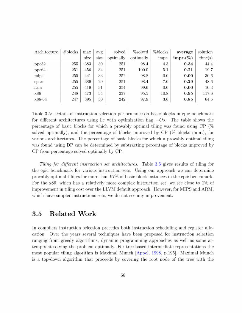
Architecture #blocks max avg solved %solved %blocks average solution

size size optimally optimally impr. impr.(%) time(s)

ppc32 255 383 30 251 98.4 4.3 0.34 44.4

ppc64 251 456 34 251 100.0 5.1 0.21 19.7

mips 255 441 33 252 98.8 0.0 0.00 30.6

sparc 255 389 29 251 98.4 7.0 0.29 48.6

arm 255 419 31 254 99.6 0.0 0.00 10.3

x86 248 473 34 237 95.5 10.8 0.95 117.6

x86-64 247 395 30 242 97.9 3.6 0.85 64.5

Table 3.5: Details of instruction selection performance on basic blocks in epic benchmark

for different architectures using llc with optimization flag −Os. The table shows the

percentage of basic blocks for which a provably optimal tiling was found using CP (%

solved optimally), and the percentage of blocks improved by CP (% blocks impr.), for

various architectures. The percentage of basic blocks for which a provably optimal tiling

was found using DP can be determined by subtracting percentage of blocks improved by

CP from percentage solved optimally by CP.

Tiling for different instruction set architectures. Table 3.5 gives results of tiling for

the epic benchmark for various instruction sets. Using our approach we can determine

provably optimal tilings for more than 97% of basic block instances in the epic benchmark.

For the x86, which has a relatively more complex instruction set, we see close to 1% of

improvement in tiling cost over the LLVM default approach. However, for MIPS and ARM,

which have simpler instructions sets, we do not see any improvement.

3.5 Related Work

In compilers instruction selection precedes both instruction scheduling and register allo-

cation. Over the years several techniques have been proposed for instruction selection

ranging from greedy algorithms, dynamic programming approaches as well as some at-

tempts at solving the problem optimally. For tree-based intermediate representations the

most popular tiling algorithm is Maximal Munch [Appel, 1998, p.195]. Maximal Munch

is a top-down algorithm that proceeds by covering the root node of the tree with the

66

largest possible tile leaving several subtrees. Each subtree is then tiled in a similar man-

ner. BURG [Fraser et al., 1992] is an early instruction selection algorithm which applies

graph matching techniques on selection trees. It decomposes the graph into trees and

applies graph grammar parsing to instruction selection by associating constant costs with

each production rule. Dynamic programming is used for optimum tiling of tree based IRs

[Appel, 1998, p.197]. The dynamic programming algorithm proceeds bottom up, finding

the cost of all children and choosing the tiling with the minimum cost. In general, least

cost instruction selection is known to be NP-complete for directed acyclic graphs [Koes and

Goldstein, 2008; Proebsting, 1998]. Thus, dynamic programming applied to DAGs does

not guarantee an optimal solution to the instruction selection problem (see Appendix B

for an example).

Among optimal approaches, Liao et al. [1995] use binate covering. Ertl [1999] presents

DBurg which is an extension of tree parsing algorithm that operates on DAGs. Bashford

and Leupers [1999][2000] present an integer linear program for code selection for multimedia

processors exploiting SIMD instructions and also a constraint logic programming formal-

ization that works on data flow graphs. The approach trades off compile time for better

code quality and works well for small instances. Kremer [1997] gives a general approach

for solving hard compiler optimization problems using integer programming. Kessler and

Bednarski [2001] present an exhaustive search method for optimal instruction selection as

an integrated approach to solve scheduling and register allocation as well. Kessler and

Bednarski [2002][2006] also present an integrated approach using integer programming to

solve instruction selection, register allocation and instruction scheduling. Their approach

scales for relatively smaller blocks of up to size forty. A related body of research integrating

several compiler optimizations yields similar results [Bednarski and Kessler, 2006; Eriksson

et al., 2008; Eriksson and Kessler, 2008]. Naik and Palsberg [2004] also present an inte-

ger linear programming approach to solving instruction selection for an embedded Ziglog

micro controller. They solve the combined problem of instruction selection and register

allocation giving an exhaustive ILP formulation for minimizing code size. Their solution

is customized for ZIL language and Z86 architecture.

Eckstein et al. [2003] present a technique which maps the instruction selection problem

for SSA graphs to partitioned Boolean quadratic problem (PBQP). The algorithm takes

into account the computational flow of the whole function. Once the SSA graph has been

mapped onto PBQP, the PBQP solver computes its grammar with minimal costs and

based on this grammar the code is generated. Tiles are defined as graph grammar rules.

67

The concept has been integrated with the CC77050 C-Compiler for NEC DSP family

which features VLIW architectures for mobile multimedia applications. The evaluation

measures the number of nodes which can be eliminated by this technique as compared to a

conventional tree pattern matcher. Schafer [2007] present a technique which uses chain-rule

matching on SSA graphs. The technique updates the control flow graph to match types

in the DAG so that the instruction selector can correctly identify matching tiles. Another

group of researchers have recently presented a combined approach for instruction selection

and register allocation [von Koch et al., 2010]. They show a size reduction of 16% and

performance improvement of 17% for a relatively uncommon ISA and the unconventional

CoSy compiler.

Koes and Goldstein [2008] present a linear-time dynamic programming algorithm which

they name NOTLIS. The algorithm operates on the expression DAG of basic blocks tiling

the nodes and computes the best choice instructions for each node in terms of the cost

function. They also present a 0-1 integer programming formulation of the problem to com-

pute the nearness to optimality of NOTLIS. The ILP formulation is incorrect as it does

not account for matching constraints (see Appendix A). Hence the conclusions based on

the results presented in their paper are not reliable. They implement NOTLIS in LLVM

2.1 compiler infrastructure targeting Intel x86 architecture and evaluate it on basic blocks

in SPEC2006, MediaBench, MiBench and VersaBench. NOTLIS optimizes for code size

and gives average improvements of 1%. Ebner et al. [2008] employ the partitioned Boolean

quadratic problem(PBQP) (known to be NP-complete) for solving the instruction selection

problem. The paper extends the instruction selector [Eckstein et al., 2003] and is primarily

concerned with identifying complex tiles within basic blocks using the SSA properties of

the intermediate representation. The implementation is done in LLVM 2.1 for an embed-

ded ARMv5 architecture and evaluated MiBench and SPECINT 2000 benchmarks. The

experiments compare the execution cycles for the object code produced by gcc, LLVM

original and the approach given by the authors and report performance improvements of

up to 10% for the SPEC benchmarks. However, the experiments were performed only

against the BURG approach, and not the newer dynamic programming approach. Our

experimental results against the BURG approach are consistent with these experimental

results.

Buchwald and Zwinkau [2010] reformulate the instruction selection problem based on

graph transformation and identify and resolve known problems with PBQP-based ap-

proaches. They also present formal foundations to verify the correctness of generated

68

code. They implement their approach within the LIBFIRM compiler and evaluate their

technique on the SPECINT 2000 benchmarks. They compare the execution times of the

benchmarks compiled with GCC 4.2.1 with their implementation and find that their tech-

nique improves execution time of the benchmarks up to 7%.

The current implementation of the instruction selector in LLVM Lattner and Avde

[2004] consists of two algorithms. The first is based on BURG and the other is a dynamic

programming instruction selection implementation. LLVM uses the SSA graphs to build

BURG trees. A BURG tree is a tree of instructions, where the children of an instruction,

I, are those that compute the operands of I, and the parent (if any) is some instruction

that uses the result of I. In the SSA graph and in real code, however, an instruction may

have multiple users, and at most one user can be represented in the tree. The need for

trees in pattern-matching rather than DAGs is one of the major limitations of the BURG

approach.

3.6 Summary

In this chapter we present a constraint programming approach for the instruction selection

problem. Our approach is optimal and scales to basic blocks of size approximately one

hundred. We implement our approach in the LLVM compiler and perform an extensive

experimental evaluation of our technique on a variety of benchmarks. The evaluation

compares the results of our optimal technique with the state-of-the-art tiling technique

implemented in LLVM, a highly tuned dynamic programming based instruction selector.

The results demonstrate that our approach slightly improves the selection cost as compared

to the state-of-the-art approach and would be feasible if where slight improvements in

selection quality improve the performance significantly.

69

Chapter 4

Cache-Conscious Data Placement

Processors make use of on-chip memory in the form of caches to improve program perfor-

mance. Caches are designed to transparently hide the latency of accessing main memory.

The effective utilization of caches requires that cache misses be minimized. A cache miss

occurs when the desired object is not found in the cache and has to be fetched from main

memory. Numerous hardware and software techniques have been proposed to minimize

the number of misses. Among the software proposals are profile-driven data placement

techniques, which carefully place data objects in memory. Optimally placing data objects

in memory to minimize cache misses is known to be NP-hard and thus assumed to be

intractable in the worst-case. Furthermore, it cannot even be approximated within reason-

able bounds. However, previous work has presented data placement algorithms that can

be effective in practice. In this chapter we use results from the theory of interval graphs

to show that it is possible to identify instances where data objects can be arranged in

memory such that there are no avoidable cache misses. Any miss that is not compulsory

or results due to the capacity of the cache is considered avoidable. For instances where a

placement is possible such that there are no avoidable misses, the placement can be de-

termined in polynomial time. We present a general algorithm for placing data in memory.

The algorithm is optimal if there exists a placement such that cache misses can be avoided

altogether. For the general case, the algorithm uses a novel graph reduction technique

to determine a good layout of the objects. On a variety of realistic cache configurations

and benchmarks, our graph-theoretic approach improves the cache hit ratio over the best

previous techniques by 9% to 21% on average.

70

4.1 Motivation

Latencies from the memory hierarchy have a significant impact on program performance.

Caches are designed to improve memory access times by copying frequently accessed data

into relatively smaller on-chip storage that is readily accessible to the processor. Since

caches are relatively much smaller in comparison to memory, cache performance is sensitive

to the layout of data and the replacement policy. Cache performance is measured as the

ratio of the number of misses—where needed objects are not in the cache—to the total

number of accesses. A cache miss can increase the latency of a memory load by an order

of magnitude.

In reality, the number and kind of cache misses depends heavily on the pattern in which

the data in memory is laid out and accessed. One kind of cache miss occurs when an object

is accessed for the first time by a program and that object had not been previously loaded

into the cache. This is called a compulsory miss. Prefetching techniques can be employed

to avoid the miss penalty resulting from compulsory misses. When an object in the cache

is replaced by another object mapped to the same set in the cache and the original object

is accessed again, a conflict miss occurs. A conflict miss can be avoided if the object had

not been evicted from the cache earlier. Capacity misses occur due to the finite size of the

cache regardless of associativity or set size. This means that when an object is accessed,

it cannot be loaded into the cache without evicting a frequently accessed object residing

in the cache. Note that conflict misses and capacity misses are not mutually exclusive.

Our focus is on improving cache performance by using profile information to determine

a placement of data objects in memory such that conflict misses can be avoided and capac-

ity misses minimized. The problem of optimally placing data in memory to minimize cache

misses is known to be intractable in the worst-case, both to solve exactly and to approxi-

mate within reasonable bounds [Petrank and Rawitz, 2002]. Bixby et al. [1994] present a

framework to find an exact placement using integer programming, but the approach does

not scale. Calder et al. [1998] present a comprehensive framework for cache conscious

data placement that utilizes a heuristic data placement algorithm. Their framework is a

proposal to modify the memory manager to make use of program profile information to

carefully lay out data in memory. The algorithm described in this thesis can replace their

technique of determining a data placement (Phase 6 in [Calder et al., 1998]).

Previous studies on data access patterns in general-purpose programs have shown that

71

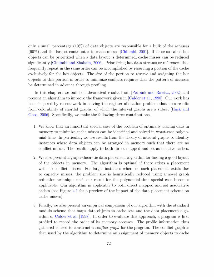
only a small percentage (10%) of data objects are responsible for a bulk of the accesses

(90%) and the largest contributor to cache misses [Chilimbi, 2001]. If these so called hot

objects can be prioritized when a data layout is determined, cache misses can be reduced

significantly [Chilimbi and Shaham, 2006]. Prioritizing hot data streams or references that

frequently repeat in the same order can be accomplished by reserving a portion of the cache

exclusively for the hot objects. The size of the portion to reserve and assigning the hot

objects to this portion in order to minimize conflicts requires that the pattern of accesses

be determined in advance through profiling.

In this chapter, we build on theoretical results from [Petrank and Rawitz, 2002] and

present an algorithm to improve the framework given in [Calder et al., 1998]. Our work has

been inspired by recent work in solving the register allocation problem that uses results

from colorability of chordal graphs, of which the interval graphs are a subset [Hack and

Goos, 2006]. Specifically, we make the following three contributions.

1. We show that an important special case of the problem of optimally placing data in

memory to minimize cache misses can be identified and solved in worst-case polyno-

mial time. In particular, we use results from the theory of interval graphs to identify

instances where data objects can be arranged in memory such that there are no

conflict misses. The results apply to both direct mapped and set associative caches.

2. We also present a graph-theoretic data placement algorithm for finding a good layout

of the objects in memory. The algorithm is optimal if there exists a placement

with no conflict misses. For larger instances where no such placement exists due

to capacity misses, the problem size is heuristically reduced using a novel graph

reduction technique until our result for the polynomial-time special case becomes

applicable. Our algorithm is applicable to both direct mapped and set associative

caches (see Figure 4.1 for a preview of the impact of the data placement scheme on

cache misses).

3. Finally, we also present an empirical comparison of our algorithm with the standard

modulo scheme that maps data objects to cache sets and the data placement algo-

rithm of Calder et al. [1998]. In order to evaluate this approach, a program is first

profiled to record the order of its memory accesses. The profile information thus

gathered is used to construct a conflict graph for the program. The conflict graph is

then used by the algorithm to determine an assignment of memory objects to cache

72

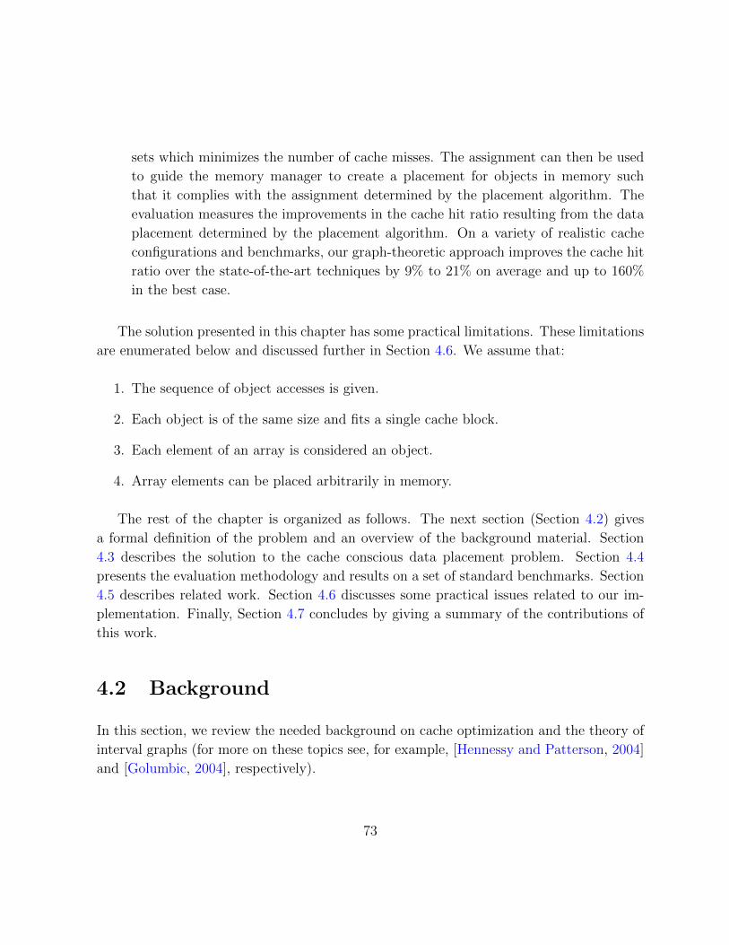
sets which minimizes the number of cache misses. The assignment can then be used

to guide the memory manager to create a placement for objects in memory such

that it complies with the assignment determined by the placement algorithm. The

evaluation measures the improvements in the cache hit ratio resulting from the data

placement determined by the placement algorithm. On a variety of realistic cache

configurations and benchmarks, our graph-theoretic approach improves the cache hit

ratio over the state-of-the-art techniques by 9% to 21% on average and up to 160%

in the best case.

The solution presented in this chapter has some practical limitations. These limitations

are enumerated below and discussed further in Section 4.6. We assume that:

1. The sequence of object accesses is given.

2. Each object is of the same size and fits a single cache block.

3. Each element of an array is considered an object.

4. Array elements can be placed arbitrarily in memory.

The rest of the chapter is organized as follows. The next section (Section 4.2) gives

a formal definition of the problem and an overview of the background material. Section

4.3 describes the solution to the cache conscious data placement problem. Section 4.4

presents the evaluation methodology and results on a set of standard benchmarks. Section

4.5 describes related work. Section 4.6 discusses some practical issues related to our im-

plementation. Finally, Section 4.7 concludes by giving a summary of the contributions of

this work.

4.2 Background

In this section, we review the needed background on cache optimization and the theory of

interval graphs (for more on these topics see, for example, [Hennessy and Patterson, 2004]

and [Golumbic, 2004], respectively).

73

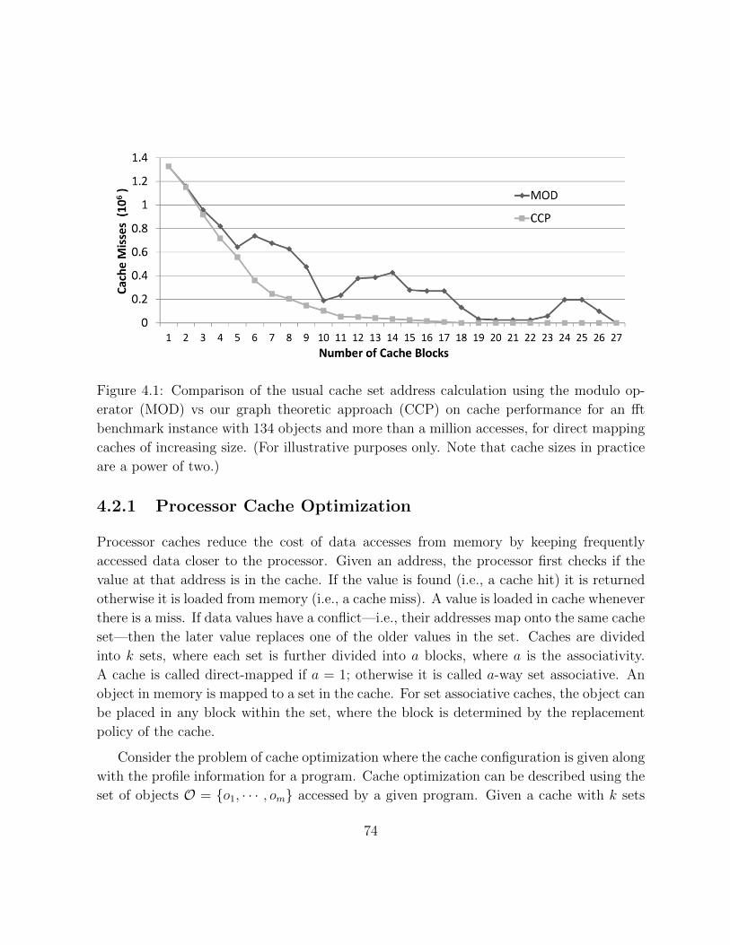
Figure 4.1: Comparison of the usual cache set address calculation using the modulo op-

erator (MOD) vs our graph theoretic approach (CCP) on cache performance for an fft

benchmark instance with 134 objects and more than a million accesses, for direct mapping

caches of increasing size. (For illustrative purposes only. Note that cache sizes in practice

are a power of two.)

4.2.1 Processor Cache Optimization

Processor caches reduce the cost of data accesses from memory by keeping frequently

accessed data closer to the processor. Given an address, the processor first checks if the

value at that address is in the cache. If the value is found (i.e., a cache hit) it is returned

otherwise it is loaded from memory (i.e., a cache miss). A value is loaded in cache whenever

there is a miss. If data values have a conflict—i.e., their addresses map onto the same cache

set—then the later value replaces one of the older values in the set. Caches are divided

into k sets, where each set is further divided into a blocks, where a is the associativity.

A cache is called direct-mapped if a = 1; otherwise it is called a-way set associative. An

object in memory is mapped to a set in the cache. For set associative caches, the object can

be placed in any block within the set, where the block is determined by the replacement

policy of the cache.

Consider the problem of cache optimization where the cache configuration is given along

with the profile information for a program. Cache optimization can be described using the

set of objects O = {o1, · · · , om} accessed by a given program. Given a cache with k sets

74

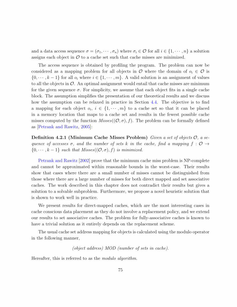
and a data access sequence σ = (σ1, · · · , σn) where σi ∈ O for all i ∈ {1, · · · , n} a solution

assigns each object in O to a cache set such that cache misses are minimized.

The access sequence is obtained by profiling the program. The problem can now be

considered as a mapping problem for all objects in O where the domain of oi ∈ O is

{0, · · · , k − 1} for all oi where i ∈ {1, · · · ,m}. A valid solution is an assignment of values

to all the objects in O. An optimal assignment would entail that cache misses are minimum

for the given sequence σ. For simplicity, we assume that each object fits in a single cache

block. The assumption simplifies the presentation of our theoretical results and we discuss

how the assumption can be relaxed in practice in Section 4.4. The objective is to find

a mapping for each object oi, i ∈ {1, · · · ,m} to a cache set so that it can be placed

in a memory location that maps to a cache set and results in the fewest possible cache

misses computed by the function Misses((O, σ), f). The problem can be formally defined

as [Petrank and Rawitz, 2005]:

Definition 4.2.1 (Minimum Cache Misses Problem) Given a set of objects O, a se-

quence of accesses σ, and the number of sets k in the cache, find a mapping f : O →{0, · · · , k − 1} such that Misses((O, σ), f) is minimized.

Petrank and Rawitz [2002] prove that the minimum cache miss problem is NP-complete

and cannot be approximated within reasonable bounds in the worst-case. Their results

show that cases where there are a small number of misses cannot be distinguished from

those where there are a large number of misses for both direct mapped and set associative

caches. The work described in this chapter does not contradict their results but gives a

solution to a solvable subproblem. Furthermore, we propose a novel heuristic solution that

is shown to work well in practice.

We present results for direct-mapped caches, which are the most interesting cases in

cache conscious data placement as they do not involve a replacement policy, and we extend

our results to set associative caches. The problem for fully-associative caches is known to

have a trivial solution as it entirely depends on the replacement scheme.

The usual cache set address mapping for objects is calculated using the modulo operator

in the following manner,

(object address) MOD (number of sets in cache).

Hereafter, this is referred to as the modulo algorithm.

75

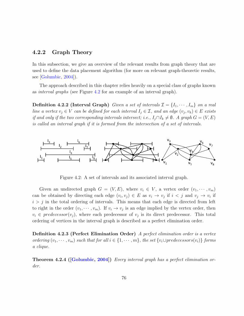
4.2.2 Graph Theory

In this subsection, we give an overview of the relevant results from graph theory that are

used to define the data placement algorithm (for more on relevant graph-theoretic results,

see [Golumbic, 2004]).

The approach described in this chapter relies heavily on a special class of graphs known

as interval graphs (see Figure 4.2 for an example of an interval graph).

Definition 4.2.2 (Interval Graph) Given a set of intervals I = {I1, · · · , Im} on a real

line a vertex vj ∈ V can be defined for each interval Ij ∈ I, and an edge (vj, vk) ∈ E exists

if and only if the two corresponding intervals intersect; i.e., Ij∩Ik 6= ∅. A graph G = (V,E)

is called an interval graph if it is formed from the intersection of a set of intervals.

Figure 4.2: A set of intervals and its associated interval graph.

Given an undirected graph G = (V,E), where vi ∈ V , a vertex order (v1, · · · , vm)

can be obtained by directing each edge (vi, vj) ∈ E as vi → vj if i < j and vj → vi if

i > j in the total ordering of intervals. This means that each edge is directed from left

to right in the order (v1, · · · , vm). If vi → vj is an edge implied by the vertex order, then

vi ∈ predecessor(vj), where each predecessor of vj is its direct predecessor. This total

ordering of vertices in the interval graph is described as a perfect elimination order.

Definition 4.2.3 (Perfect Elimination Order) A perfect elimination order is a vertex

ordering (v1, · · · , vm) such that for all i ∈ {1, · · · ,m}, the set {vi∪predecessors(vi)} forms

a clique.

Theorem 4.2.4 ([Golumbic, 2004]) Every interval graph has a perfect elimination or-

der.

76

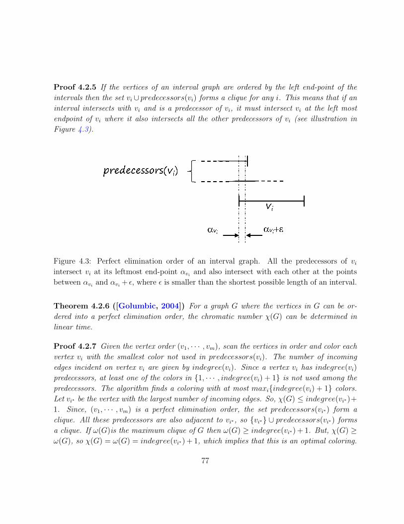
Proof 4.2.5 If the vertices of an interval graph are ordered by the left end-point of the

intervals then the set vi ∪ predecessors(vi) forms a clique for any i. This means that if an

interval intersects with vi and is a predecessor of vi, it must intersect vi at the left most

endpoint of vi where it also intersects all the other predecessors of vi (see illustration in

Figure 4.3).

Figure 4.3: Perfect elimination order of an interval graph. All the predecessors of viintersect vi at its leftmost end-point αvi and also intersect with each other at the points

between αvi and αvi + ε, where ε is smaller than the shortest possible length of an interval.

Theorem 4.2.6 ([Golumbic, 2004]) For a graph G where the vertices in G can be or-

dered into a perfect elimination order, the chromatic number χ(G) can be determined in

linear time.

Proof 4.2.7 Given the vertex order (v1, · · · , vm), scan the vertices in order and color each

vertex vi with the smallest color not used in predecessors(vi). The number of incoming

edges incident on vertex vi are given by indegree(vi). Since a vertex vi has indegree(vi)

predecessors, at least one of the colors in {1, · · · , indegree(vi) + 1} is not used among the

predecessors. The algorithm finds a coloring with at most maxi{indegree(vi) + 1} colors.

Let vi∗ be the vertex with the largest number of incoming edges. So, χ(G) ≤ indegree(vi∗)+

1. Since, (v1, · · · , vm) is a perfect elimination order, the set predecessors(vi∗) form a

clique. All these predecessors are also adjacent to vi∗, so {vi∗} ∪ predecessors(vi∗) forms

a clique. If ω(G)is the maximum clique of G then ω(G) ≥ indegree(vi∗) + 1. But, χ(G) ≥ω(G), so χ(G) = ω(G) = indegree(vi∗) + 1, which implies that this is an optimal coloring.

77

Figure 4.4: Example of a perfect elimination order and coloring.

Example 4.2.8 Consider the interval graph shown in Figure 4.2. A perfect elimination

for this graph is shown in Figure 4.4; i.e., v1, v2, . . . , v8. A coloring for this graph is also

shown in Figure 4.4. For example, v1 is receives color 1 and v5 receives color 3.

Theorem 4.2.9 ([Golumbic, 2004]) For a graph G where the vertices in G can be or-

dered into a perfect elimination order, the maximal cliques can be found in linear time.

The proof of this theorem is given in [Golumbic, 2004] which gives an algorithm to find

all the maximal cliques in the graph.

Definition 4.2.10 (Edge Contraction) Given an edge e = (u, v) in graph G, contract-

ing the edge e results in an induced subgraph G′ in which the edge e is removed and the

two vertices u and v are merged. All edges incident to u and v in G become incident to the

merged vertex.

Theorem 4.2.11 ([Golumbic, 2004]) An induced subgraph G′ of an interval graph G,

resulting from contracting an edge, is also an interval graph.

Proof 4.2.12 Let (u, v) be the edge to be contracted in G. Consider the interval represen-

tation of G where Iu and Iv represent the two intervals corresponding to u and v. Replace

the intervals Iu and Iv with Iuv where the left end-point of Iuv is the left-most point in Iuor Iv and the right-most end point of Iuv is the right-most point in Iu or Iv. Now remove

Iu and Iv and add Iuv to the interval representation. The intersection graph of the new set

of intervals is G′.

78

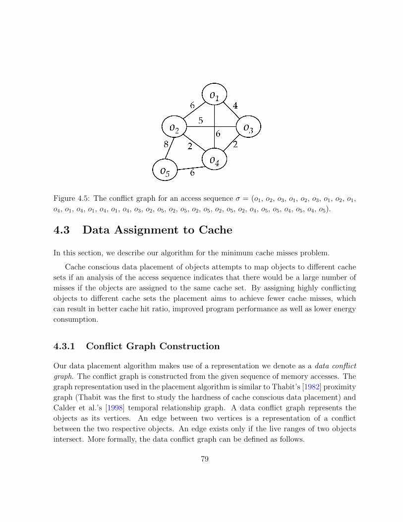
Figure 4.5: The conflict graph for an access sequence σ = (o1, o2, o3, o1, o2, o3, o1, o2, o1,

o4, o1, o4, o1, o4, o1, o4, o3, o2, o5, o2, o5, o2, o5, o2, o5, o2, o4, o5, o5, o4, o5, o4, o5).

4.3 Data Assignment to Cache

In this section, we describe our algorithm for the minimum cache misses problem.

Cache conscious data placement of objects attempts to map objects to different cache

sets if an analysis of the access sequence indicates that there would be a large number of

misses if the objects are assigned to the same cache set. By assigning highly conflicting

objects to different cache sets the placement aims to achieve fewer cache misses, which

can result in better cache hit ratio, improved program performance as well as lower energy

consumption.

4.3.1 Conflict Graph Construction

Our data placement algorithm makes use of a representation we denote as a data conflict

graph. The conflict graph is constructed from the given sequence of memory accesses. The

graph representation used in the placement algorithm is similar to Thabit’s [1982] proximity

graph (Thabit was the first to study the hardness of cache conscious data placement) and

Calder et al.’s [1998] temporal relationship graph. A data conflict graph represents the

objects as its vertices. An edge between two vertices is a representation of a conflict

between the two respective objects. An edge exists only if the live ranges of two objects

intersect. More formally, the data conflict graph can be defined as follows.

79

Definition 4.3.1 (Data Conflict Graph) Let O = {o1, · · · , om} be the set of objects

referenced in a program. For a sequence of accesses σ = (σ1, · · · , σn), where σi ∈ O for

all i ∈ {1, · · · , n}, the data conflict graph can be given by an undirected graph G = (V,E)

where |V | = m and each vertex vi ∈ V represents the memory object oi and an edge

(vi, vj) ∈ E exists if and only if mapping oi and oj to the same cache block results in one

or more conflict misses.

An edge between two vertices vi and vj means that there is a subsequence in σ of

the form σi = (oi, · · · , oj, · · · , oi) or σj = (oj, · · · , oi, · · · , oj). A data conflict graph is

an undirected graph where the labels on the edges are weights representing the degree of

conflict between the connected objects.

Definition 4.3.2 (Conflict Graph Edge Weight) Each edge (vi, vj) ∈ E in the data

conflict graph is assigned a weight which is one less than the number of unique transitions

of the form (oi, · · · , oj) or (oj, · · · , oi) in the sequence σ, where oi and oj exist only at the

start and end of the subsequences.

Example 4.3.3 Consider the edge between o1 and o3 in the conflict graph shown in Figure

4.5. If the instances of all objects other than o1 and o3 are removed from the access sequence

σ we get a subsequence (o1, o3, o1, o3, o1, o1, o1, o1, o1, o3). Now assume that both objects o1and o3 are mapped to the same cache block and no other objects are mapped to that block.

The first access of o1 results in a compulsory miss and so does the first access of o3. The

second access of o1 results in the first conflict miss. The subsequent access of o3 results in

another conflict miss making it two conflict misses. The next access of o1 results in another

conflict miss increasing the total to three. The next four accesses of o1 do not result in any

misses. The last access of o3 results in another conflict miss, resulting in a total of four

conflicts between o1 and o3.

The edge weight of (vi, vj) represents the number of times the two objects will be

swapped out of the cache if they are assigned to the same cache block and no other object

is assigned to that block. The weight of each edge is intended to capture the number of

conflict misses of the two objects represented by the vertices if the conflict was allowed to

exist during execution of the program. Alternatively, but equivalently, the weight is the

number of alternating occurrences of oi and oj in σ, other than the first occurrence, which

80

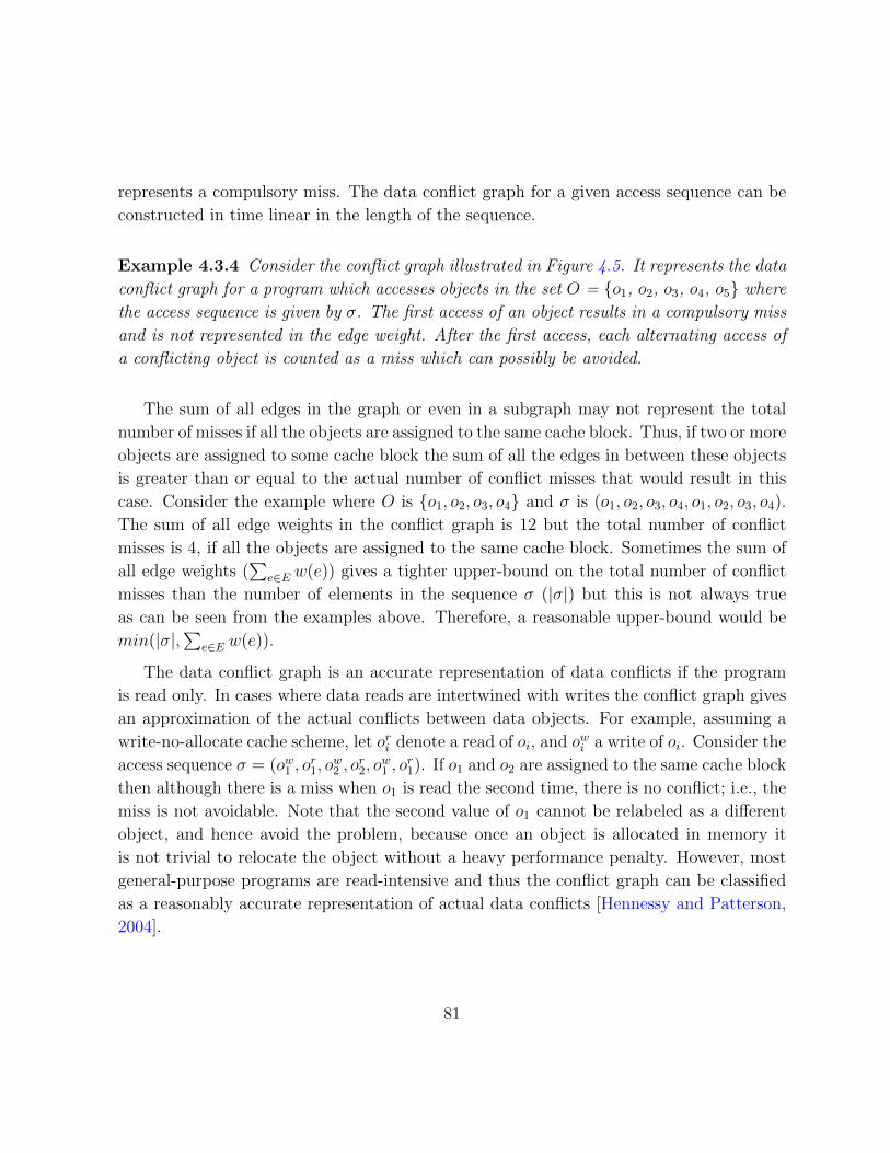
represents a compulsory miss. The data conflict graph for a given access sequence can be

constructed in time linear in the length of the sequence.

Example 4.3.4 Consider the conflict graph illustrated in Figure 4.5. It represents the data

conflict graph for a program which accesses objects in the set O = {o1, o2, o3, o4, o5} where

the access sequence is given by σ. The first access of an object results in a compulsory miss

and is not represented in the edge weight. After the first access, each alternating access of

a conflicting object is counted as a miss which can possibly be avoided.

The sum of all edges in the graph or even in a subgraph may not represent the total

number of misses if all the objects are assigned to the same cache block. Thus, if two or more

objects are assigned to some cache block the sum of all the edges in between these objects

is greater than or equal to the actual number of conflict misses that would result in this

case. Consider the example where O is {o1, o2, o3, o4} and σ is (o1, o2, o3, o4, o1, o2, o3, o4).

The sum of all edge weights in the conflict graph is 12 but the total number of conflict

misses is 4, if all the objects are assigned to the same cache block. Sometimes the sum of

all edge weights (∑

e∈E w(e)) gives a tighter upper-bound on the total number of conflict

misses than the number of elements in the sequence σ (|σ|) but this is not always true

as can be seen from the examples above. Therefore, a reasonable upper-bound would be

min(|σ|,∑

e∈E w(e)).

The data conflict graph is an accurate representation of data conflicts if the program

is read only. In cases where data reads are intertwined with writes the conflict graph gives

an approximation of the actual conflicts between data objects. For example, assuming a

write-no-allocate cache scheme, let ori denote a read of oi, and owi a write of oi. Consider the

access sequence σ = (ow1 , or1, o

w2 , o

r2, o

w1 , o

r1). If o1 and o2 are assigned to the same cache block

then although there is a miss when o1 is read the second time, there is no conflict; i.e., the

miss is not avoidable. Note that the second value of o1 cannot be relabeled as a different

object, and hence avoid the problem, because once an object is allocated in memory it

is not trivial to relocate the object without a heavy performance penalty. However, most

general-purpose programs are read-intensive and thus the conflict graph can be classified

as a reasonably accurate representation of actual data conflicts [Hennessy and Patterson,

2004].

81

4.3.2 Conflict Graph Classification

Our central insight is that the data conflict graph represents an intersection of intervals.

Consider an interval beginning from the first occurrence of an object in the data access

sequence and ending at its last occurrence. We call it the live range of the object. Now

consider the set of intervals for all objects representing the live ranges of the respective

objects. A conflict can only occur if two objects are alive at the same time during program

execution; i.e., their live ranges intersect. The data conflict graph can now be formally

classified as an interval graph. This classification can then be used to simplify the problem

of data placement.

Theorem 4.3.5 Given a sequence of data accesses, the data conflict graph of a program

is an interval graph.

Proof 4.3.6 Given that σ is a finite and totally ordered sequence, each object has a well

defined first and last occurrence in σ. Also given that exactly one object occupies each

position in the sequence σ, each object can be represented by a unique interval from the

first to the last occurrence of that object in σ. Since each object can be represented by an

interval given an access sequence σ and a conflict miss only occurs if two intervals intersect,

the data conflict graph is an intersection graph of intervals.

Once it is established that the data conflict graph is an interval graph, the results

which are applicable to interval graphs can also be applied to the data conflict graph.

The immediate consequences are that problems such as colorability and max-clique can be

computed in linear time for the data conflict graph. Colorability of a conflict graph can

be defined as follows.

Corollary 4.3.7 Colorability of a data conflict graph of any program can be determined

in linear time.

Proof 4.3.8 By Theorem 4.3.5 the data conflict graph is an intersection graph of intervals.

By Theorem 4.2.4 interval graphs can be represented by a perfect elimination order. Finally,

by Theorem 4.2.6 the chromatic number for a graph represented by a perfect elimination

order can be determined in linear time.

82

Corollary 4.3.9 Maximal cliques of a data conflict graph can be listed in linear time.

Proof 4.3.10 Proof is similar to Corollary 4.3.7, but using Theorem 4.2.9.

Corollary 4.3.11 Size of the maximum clique of a data conflict graph can be determined

in linear time.

Proof 4.3.12 For interval graphs the size of the maximum clique is equal to its chromatic

number. Since the chromatic number of the data conflict graph can be determined in linear

time by Corollary 4.3.7, so can the size of the maximum clique.

We next apply our results on conflict graphs to the minimum cache misses problem.

Theorem 4.3.13 The chromatic number for the conflict graph gives the minimum number

of cache sets required to achieve zero conflict misses for a given sequence.

Proof 4.3.14 The chromatic number gives the minimum number of colors needed to color

the conflict graph such that no two adjacent vertices have the same color. If all vertices

having the same color are considered, and the respective objects are placed in the same

cache set, since there are no edges between vertices of the same color, no conflict misses

would result. Similarly, if all vertices are placed in a cache with at least χ(G) sets, the

result is zero conflict misses.

A consequence of the theorem is that if a placement results in zero conflict misses, there

are no edges between objects which have been assigned to the same cache block.

Example 4.3.15 Consider once again Example 4.3.4 and the conflict graph shown in

Figure 4.5. The chromatic number of the conflict graph is four. Thus, if there are four

blocks to assign the five objects a placement can be found which would result in zero conflict

misses. For example, consider a direct mapped cache with four blocks. If o1, o2, o3, and o4are all mapped to different blocks and o5 is placed either with o1 or o3, this would result in

zero conflict misses.

83

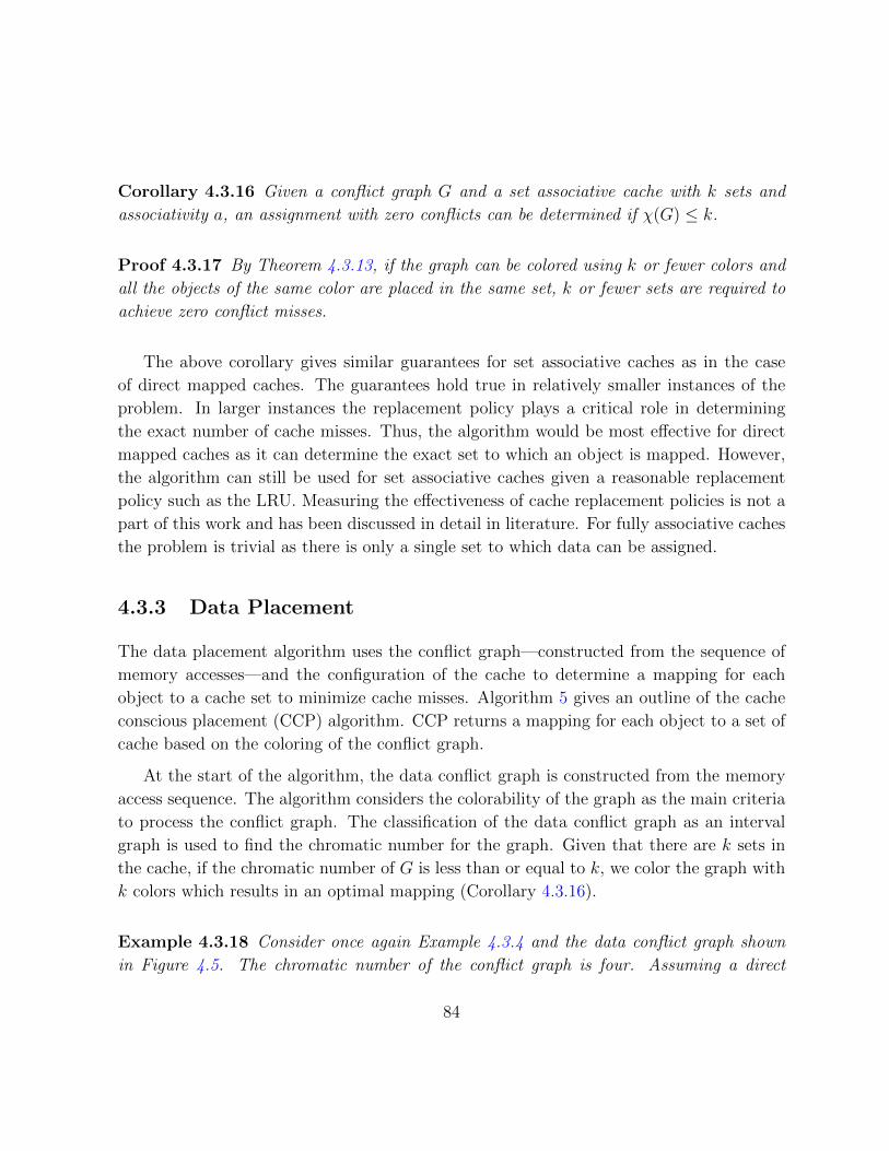
Corollary 4.3.16 Given a conflict graph G and a set associative cache with k sets and

associativity a, an assignment with zero conflicts can be determined if χ(G) ≤ k.

Proof 4.3.17 By Theorem 4.3.13, if the graph can be colored using k or fewer colors and

all the objects of the same color are placed in the same set, k or fewer sets are required to

achieve zero conflict misses.

The above corollary gives similar guarantees for set associative caches as in the case

of direct mapped caches. The guarantees hold true in relatively smaller instances of the

problem. In larger instances the replacement policy plays a critical role in determining

the exact number of cache misses. Thus, the algorithm would be most effective for direct

mapped caches as it can determine the exact set to which an object is mapped. However,

the algorithm can still be used for set associative caches given a reasonable replacement

policy such as the LRU. Measuring the effectiveness of cache replacement policies is not a

part of this work and has been discussed in detail in literature. For fully associative caches

the problem is trivial as there is only a single set to which data can be assigned.

4.3.3 Data Placement

The data placement algorithm uses the conflict graph—constructed from the sequence of

memory accesses—and the configuration of the cache to determine a mapping for each

object to a cache set to minimize cache misses. Algorithm 5 gives an outline of the cache

conscious placement (CCP) algorithm. CCP returns a mapping for each object to a set of

cache based on the coloring of the conflict graph.

At the start of the algorithm, the data conflict graph is constructed from the memory

access sequence. The algorithm considers the colorability of the graph as the main criteria

to process the conflict graph. The classification of the data conflict graph as an interval

graph is used to find the chromatic number for the graph. Given that there are k sets in

the cache, if the chromatic number of G is less than or equal to k, we color the graph with

k colors which results in an optimal mapping (Corollary 4.3.16).

Example 4.3.18 Consider once again Example 4.3.4 and the data conflict graph shown

in Figure 4.5. The chromatic number of the conflict graph is four. Assuming a direct

84

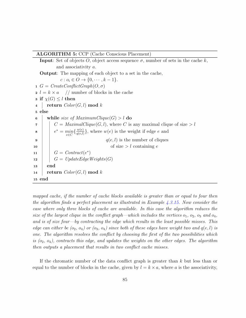
ALGORITHM 5: CCP (Cache Conscious Placement)

Input: Set of objects O, object access sequence σ, number of sets in the cache k,

and associativity a.

Output: The mapping of each object to a set in the cache,

c : oi ∈ O → {0, · · · , k − 1}.1 G = CreateConflictGraph(O, σ)

2 l = k × a // number of blocks in the cache

3 if χ(G) ≤ l then

4 return Color(G, l) mod k

5 else

6 while size of MaximumClique(G) > l do

7 C = MaximalClique(G, l), where C is any maximal clique of size > l

8 e∗ = mine∈C{ w(e)q(e,l)}, where w(e) is the weight if edge e and

9 q(e, l) is the number of cliques

10 of size > l containing e

11 G = Contract(e∗)

12 G = UpdateEdgeWeights(G)

13 end

14 return Color(G, l) mod k

15 end

mapped cache, if the number of cache blocks available is greater than or equal to four then

the algorithm finds a perfect placement as illustrated in Example 4.3.15. Now consider the

case where only three blocks of cache are available. In this case the algorithm reduces the

size of the largest clique in the conflict graph—which includes the vertices o1, o2, o3 and o4,

and is of size four—by contracting the edge which results in the least possible misses. This

edge can either be (o2, o4) or (o3, o4) since both of these edges have weight two and q(e, l) is

one. The algorithm resolves the conflict by choosing the first of the two possibilities which

is (o2, o4), contracts this edge, and updates the weights on the other edges. The algorithm

then outputs a placement that results in two conflict cache misses.

If the chromatic number of the data conflict graph is greater than k but less than or

equal to the number of blocks in the cache, given by l = k×a, where a is the associativity,

85

CCP colors the graph using l or fewer colors and the final mapping to cache sets is de-

termined by taking the l-coloring and applying the mod operator to distribute the objects

equally over cache sets. This gives a better placement than reducing the size of the graph

to make it k-colorable which is also an alternative heuristic but is worse in terms of time

complexity than the constant time mod. The coloring algorithm has linear time complexity

(see Algorithm 6). If the chromatic number of the data conflict graph is greater than the

number of cache blocks l, the algorithm heuristically selects vertices of the conflict graph

to merge until the graph becomes l-colorable. The objective of this exercise is to merge

vertices connected by the least-weighted edges.

In order to make the graph colorable the size of large cliques is systematically decreased.

This is because the chromatic number of an interval graph is equal to the size of the largest

clique in the graph. Decreasing the size of the largest clique decreases the chromatic number

of the graph. A list of all the maximal cliques that are of size greater than the number

of blocks in the cache l is determined and iteratively reduced by merging vertices in each

one of these cliques until the maximum clique in the reduced graph is of size l. A maximal

clique is not the maximum clique in the graph but it is not a part of a larger clique. The

maximal cliques in an interval graph can be listed in linear time (see Theorem 4.2.9).

Once a clique of size greater than the number of blocks in the cache l has been identified,

the next step is to choose the best possible edge to contract (merge the two vertices

connected by it) and reduce the size of the clique by one. To find the edge which would be

the overall optimal choice is a hard problem if there are two or more overlapping cliques

of size greater than l in the data conflict graph. In such cases the idea is to reduce the

size of as many maximal cliques as possible by contracting edges with the least combined

weight (Contract(e∗)). To that end, an edge e∗ is selected for contraction which minimizes

the fraction w(e)q(e,l)

where w(e) is the weight of the edge and q(e, l) are the number of cliques

larger than size l that include e as an edge. Once the edge is contracted the weights of all

the edges adjacent to the contracted edges are recomputed (UpdateEdgeWeights(G)). This

recomputation reflects the change in the number of misses between the newly combined

objects and other objects. The resulting graph is still an interval graph, as contracting an

edge can be seen as merging two intervals. The process is repeated by choosing another

edge until the size of the reduced clique is equal to l.

After all the large cliques have been reduced to size l, the resulting graph (which is still

an interval graph, see Theorem 4.2.11) can be colored using the interval graph coloring

86

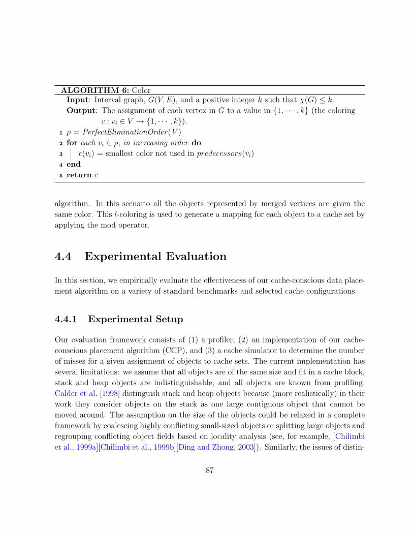
ALGORITHM 6: ColorInput: Interval graph, G(V,E), and a positive integer k such that χ(G) ≤ k.

Output: The assignment of each vertex in G to a value in {1, · · · , k} (the coloring

c : vi ∈ V → {1, · · · , k}).1 ρ = PerfectEliminationOrder(V )

2 for each vi ∈ ρ; in increasing order do

3 c(vi) = smallest color not used in predecessors(vi)

4 end

5 return c

algorithm. In this scenario all the objects represented by merged vertices are given the

same color. This l-coloring is used to generate a mapping for each object to a cache set by

applying the mod operator.

4.4 Experimental Evaluation

In this section, we empirically evaluate the effectiveness of our cache-conscious data place-

ment algorithm on a variety of standard benchmarks and selected cache configurations.

4.4.1 Experimental Setup

Our evaluation framework consists of (1) a profiler, (2) an implementation of our cache-

conscious placement algorithm (CCP), and (3) a cache simulator to determine the number

of misses for a given assignment of objects to cache sets. The current implementation has

several limitations: we assume that all objects are of the same size and fit in a cache block,

stack and heap objects are indistinguishable, and all objects are known from profiling.

Calder et al. [1998] distinguish stack and heap objects because (more realistically) in their

work they consider objects on the stack as one large contiguous object that cannot be

moved around. The assumption on the size of the objects could be relaxed in a complete

framework by coalescing highly conflicting small-sized objects or splitting large objects and

regrouping conflicting object fields based on locality analysis (see, for example, [Chilimbi

et al., 1999a][Chilimbi et al., 1999b][Ding and Zhong, 2003]). Similarly, the issues of distin-

87

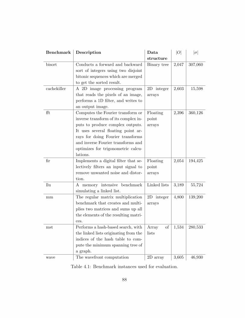
Benchmark Description Data

structure

|O| |σ|

bisort Conducts a forward and backward

sort of integers using two disjoint

bitonic sequences which are merged

to get the sorted result.

Binary tree 2,047 307,060

cachekiller A 2D image processing program

that reads the pixels of an image,

performs a 1D filter, and writes to

an output image.

2D integer

arrays

2,603 15,598

fft Computes the Fourier transform or

inverse transform of its complex in-

puts to produce complex outputs.

It uses several floating point ar-

rays for doing Fourier transforms

and inverse Fourier transforms and

optimizes for trigonometric calcu-

lations.

Floating

point

arrays

2,396 360,126

fir Implements a digital filter that se-

lectively filters an input signal to

remove unwanted noise and distor-

tion.

Floating

point

arrays

2,054 194,425

llu A memory intensive benchmark

simulating a linked list.

Linked lists 3,189 55,724

mm The regular matrix multiplication

benchmark that creates and multi-

plies two matrices and sums up all

the elements of the resulting matri-

ces.

2D integer

arrays

4,800 139,200

mst Performs a hash-based search, with

the linked lists originating from the

indices of the hash table to com-

pute the minimum spanning tree of

a graph.

Array of

lists

1,534 280,533

wave The wavefront computation 2D array 3,605 46,930

Table 4.1: Benchmark instances used for evaluation.

88

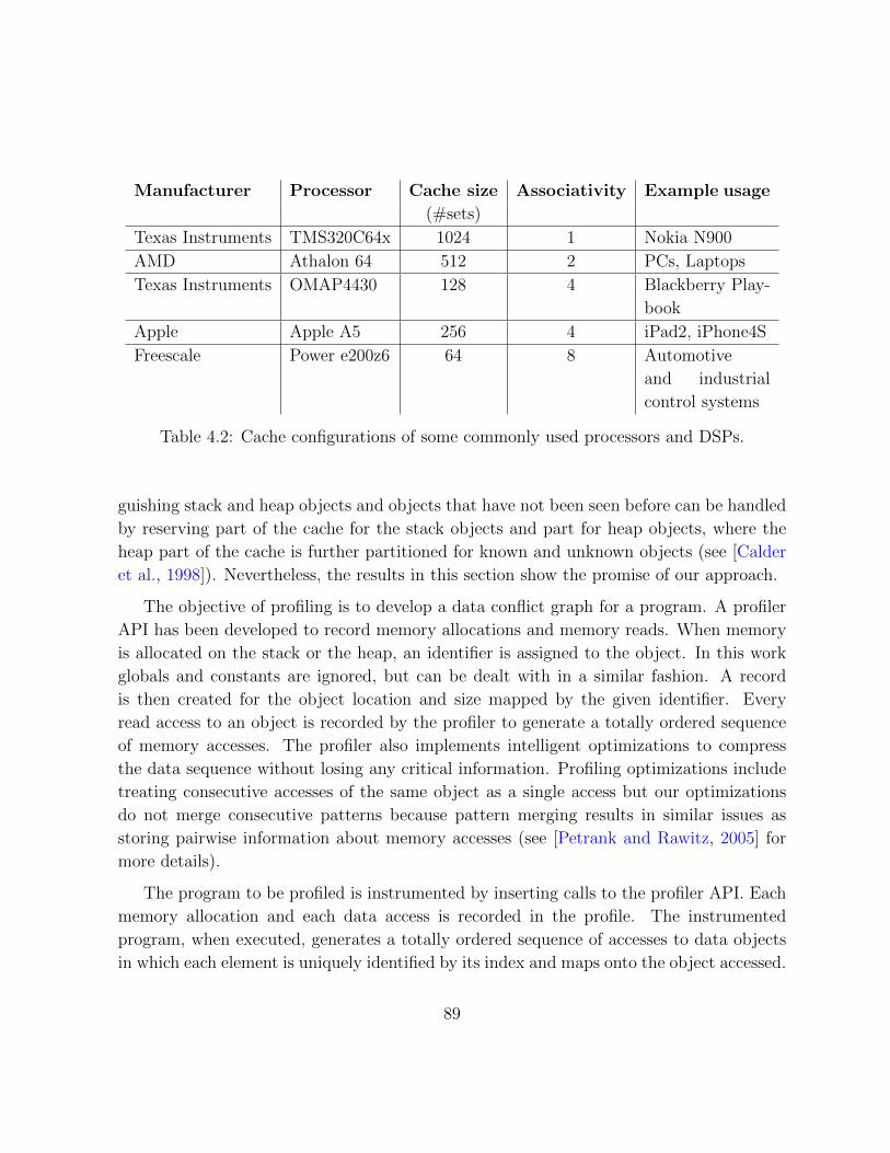
Manufacturer Processor Cache size Associativity Example usage

(#sets)

Texas Instruments TMS320C64x 1024 1 Nokia N900

AMD Athalon 64 512 2 PCs, Laptops

Texas Instruments OMAP4430 128 4 Blackberry Play-

book

Apple Apple A5 256 4 iPad2, iPhone4S

Freescale Power e200z6 64 8 Automotive

and industrial

control systems

Table 4.2: Cache configurations of some commonly used processors and DSPs.

guishing stack and heap objects and objects that have not been seen before can be handled

by reserving part of the cache for the stack objects and part for heap objects, where the

heap part of the cache is further partitioned for known and unknown objects (see [Calder

et al., 1998]). Nevertheless, the results in this section show the promise of our approach.

The objective of profiling is to develop a data conflict graph for a program. A profiler

API has been developed to record memory allocations and memory reads. When memory

is allocated on the stack or the heap, an identifier is assigned to the object. In this work

globals and constants are ignored, but can be dealt with in a similar fashion. A record

is then created for the object location and size mapped by the given identifier. Every

read access to an object is recorded by the profiler to generate a totally ordered sequence

of memory accesses. The profiler also implements intelligent optimizations to compress

the data sequence without losing any critical information. Profiling optimizations include

treating consecutive accesses of the same object as a single access but our optimizations

do not merge consecutive patterns because pattern merging results in similar issues as

storing pairwise information about memory accesses (see [Petrank and Rawitz, 2005] for

more details).

The program to be profiled is instrumented by inserting calls to the profiler API. Each

memory allocation and each data access is recorded in the profile. The instrumented

program, when executed, generates a totally ordered sequence of accesses to data objects

in which each element is uniquely identified by its index and maps onto the object accessed.

89

A cache simulator was developed to accurately compute the cache hit ratio. The cache

simulator accepts a memory access sequence, a cache configuration and a mapping of

objects to sets in the cache and outputs the number of misses resulting from the given

assignment. The simulator computes the misses for each cache block by looking up the

objects assigned to the block and traversing the data access sequence. The summation of

misses from all cache sets determines the total number of misses.

In our experiments, the least recently used (LRU) cache block replacement policy was

used for set associative caches, as LRU outperforms other popular replacement policies

[Hennessy and Patterson, 2004, p. 400]. In the LRU policy, when all blocks in a cache set

are occupied and a memory access causes a data load into the cache, the block in the set

whose last occurrence appears earliest in the access sequence is replaced.

We evaluated our CCP algorithm (Algorithm 5) for cache hit ratio and compared

our algorithm to the standard modulo algorithm that maps data objects to cache sets,

denoted here as MOD, and the data placement algorithm of Calder et al. [1998], denoted

here as CKJA. MOD evenly distributes objects over the cache blocks simply by a modulo

operation on the virtual address of the location of an object in memory. MOD was chosen

for comparison as it (or its variants) is the algorithm of choice in most cache system

implementations and is easy to implement in hardware. CKJA was chosen for comparison

as, to the best of our knowledge, it represents the state-of-the-art in software approaches

using profile-driven data placement. Both CCP and CKJA use profiling to create a graph

that represents memory objects and conflicts between these objects. However, the way the

algorithms process the graphs differs significantly. CCP coalesces vertices to put objects

into the same cache block until the meta-vertices can be assigned to the cache with zero

conflicts, whereas CKJA coalesces vertices to put objects into different cache blocks until

the graph is a single meta-vertex. As well, CKJA is designed for direct mapped caches,

whereas CCP has also been extended to set associative caches.

4.4.2 Experimental Results & Analysis

Eight benchmarks from a variety of benchmark suites have been selected for evaluating

the effectiveness of CCP. These benchmarks are selected because of their intensive use of

memory and a diverse set of data access patterns. Two of these benchmarks, bisort and mst,

are part of the Olden benchmark suite which has been popular for data structure layout

90

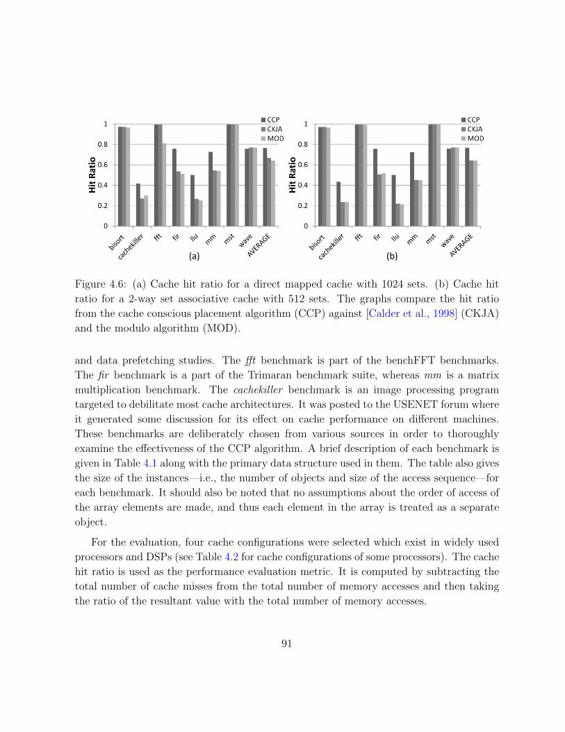
Figure 4.6: (a) Cache hit ratio for a direct mapped cache with 1024 sets. (b) Cache hit

ratio for a 2-way set associative cache with 512 sets. The graphs compare the hit ratio

from the cache conscious placement algorithm (CCP) against [Calder et al., 1998] (CKJA)

and the modulo algorithm (MOD).

and data prefetching studies. The fft benchmark is part of the benchFFT benchmarks.

The fir benchmark is a part of the Trimaran benchmark suite, whereas mm is a matrix

multiplication benchmark. The cachekiller benchmark is an image processing program

targeted to debilitate most cache architectures. It was posted to the USENET forum where

it generated some discussion for its effect on cache performance on different machines.

These benchmarks are deliberately chosen from various sources in order to thoroughly

examine the effectiveness of the CCP algorithm. A brief description of each benchmark is

given in Table 4.1 along with the primary data structure used in them. The table also gives

the size of the instances—i.e., the number of objects and size of the access sequence—for

each benchmark. It should also be noted that no assumptions about the order of access of

the array elements are made, and thus each element in the array is treated as a separate

object.

For the evaluation, four cache configurations were selected which exist in widely used

processors and DSPs (see Table 4.2 for cache configurations of some processors). The cache

hit ratio is used as the performance evaluation metric. It is computed by subtracting the

total number of cache misses from the total number of memory accesses and then taking

the ratio of the resultant value with the total number of memory accesses.

91

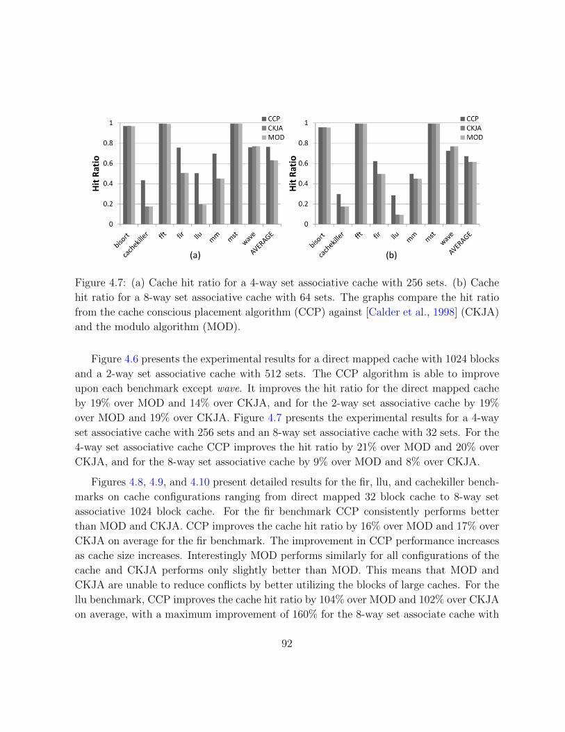
Figure 4.7: (a) Cache hit ratio for a 4-way set associative cache with 256 sets. (b) Cache

hit ratio for a 8-way set associative cache with 64 sets. The graphs compare the hit ratio

from the cache conscious placement algorithm (CCP) against [Calder et al., 1998] (CKJA)

and the modulo algorithm (MOD).

Figure 4.6 presents the experimental results for a direct mapped cache with 1024 blocks

and a 2-way set associative cache with 512 sets. The CCP algorithm is able to improve

upon each benchmark except wave. It improves the hit ratio for the direct mapped cache

by 19% over MOD and 14% over CKJA, and for the 2-way set associative cache by 19%

over MOD and 19% over CKJA. Figure 4.7 presents the experimental results for a 4-way

set associative cache with 256 sets and an 8-way set associative cache with 32 sets. For the

4-way set associative cache CCP improves the hit ratio by 21% over MOD and 20% over

CKJA, and for the 8-way set associative cache by 9% over MOD and 8% over CKJA.

Figures 4.8, 4.9, and 4.10 present detailed results for the fir, llu, and cachekiller bench-

marks on cache configurations ranging from direct mapped 32 block cache to 8-way set

associative 1024 block cache. For the fir benchmark CCP consistently performs better

than MOD and CKJA. CCP improves the cache hit ratio by 16% over MOD and 17% over

CKJA on average for the fir benchmark. The improvement in CCP performance increases

as cache size increases. Interestingly MOD performs similarly for all configurations of the

cache and CKJA performs only slightly better than MOD. This means that MOD and

CKJA are unable to reduce conflicts by better utilizing the blocks of large caches. For the

llu benchmark, CCP improves the cache hit ratio by 104% over MOD and 102% over CKJA

on average, with a maximum improvement of 160% for the 8-way set associate cache with

92

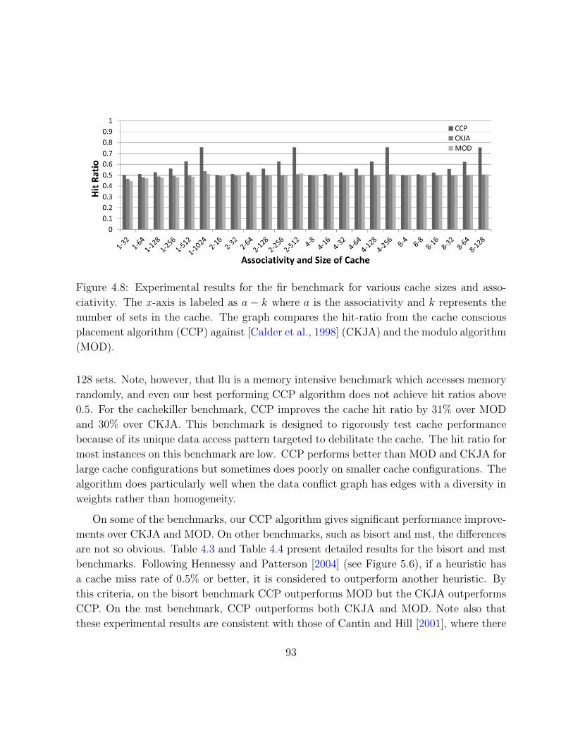
Figure 4.8: Experimental results for the fir benchmark for various cache sizes and asso-

ciativity. The x-axis is labeled as a − k where a is the associativity and k represents the

number of sets in the cache. The graph compares the hit-ratio from the cache conscious

placement algorithm (CCP) against [Calder et al., 1998] (CKJA) and the modulo algorithm

(MOD).

128 sets. Note, however, that llu is a memory intensive benchmark which accesses memory

randomly, and even our best performing CCP algorithm does not achieve hit ratios above

0.5. For the cachekiller benchmark, CCP improves the cache hit ratio by 31% over MOD

and 30% over CKJA. This benchmark is designed to rigorously test cache performance

because of its unique data access pattern targeted to debilitate the cache. The hit ratio for

most instances on this benchmark are low. CCP performs better than MOD and CKJA for

large cache configurations but sometimes does poorly on smaller cache configurations. The

algorithm does particularly well when the data conflict graph has edges with a diversity in

weights rather than homogeneity.

On some of the benchmarks, our CCP algorithm gives significant performance improve-

ments over CKJA and MOD. On other benchmarks, such as bisort and mst, the differences

are not so obvious. Table 4.3 and Table 4.4 present detailed results for the bisort and mst

benchmarks. Following Hennessy and Patterson [2004] (see Figure 5.6), if a heuristic has

a cache miss rate of 0.5% or better, it is considered to outperform another heuristic. By

this criteria, on the bisort benchmark CCP outperforms MOD but the CKJA outperforms

CCP. On the mst benchmark, CCP outperforms both CKJA and MOD. Note also that

these experimental results are consistent with those of Cantin and Hill [2001], where there

93

Figure 4.9: Experimental results for the llu benchmark for various cache sizes and asso-

ciativity. The x-axis is labeled as a − k where a is the associativity and k represents the

number of sets in the cache. The graph compares the hit-ratio from the cache conscious

placement algorithm (CCP) against [Calder et al., 1998] (CKJA) and the modulo algorithm

(MOD).

are small improvements in miss rates as associativity is increased and more significant

improvements in miss rates as cache size is increased.

4.5 Related Work

A significant amount of research has been done to optimize caches. Both hardware and

software techniques have been employed for improving cache utilization. Hardware en-

hancements to caches include increased associativity for reducing conflicts between objects

mapped to the same set, multibanked caches to increase cache bandwidth and multi-level

caches to reduce miss penalty, among others (see, e.g., [Hennessy and Patterson, 2004]).

Software techniques, including compile-time optimizations as well as run-time optimiza-

tions, have also been useful in reducing cache misses. Among the most well known ones

are prefetching [Jula and Rauchwerger, 2009], loop interchange [Wolf et al., 1998], code

and data rearrangement [Ding and Kennedy, 1999; Prokopski and Verbrugge, 2008], block-

ing [Jin et al., 2001], and structure splitting [Chilimbi and Larus, 1998; Chilimbi et al.,

1999a; Chilimbi and Hirzel, 2002; Chilimbi et al., 1999b; Lattner and Adve, 2005]. Re-

94

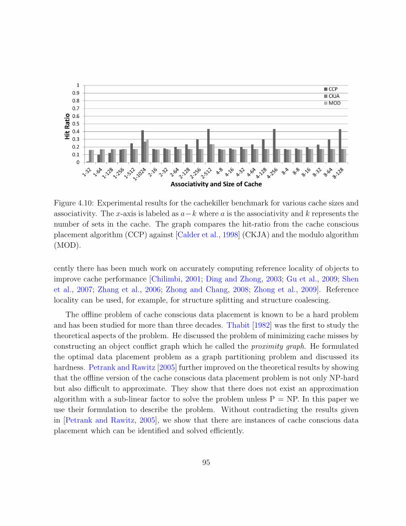
Figure 4.10: Experimental results for the cachekiller benchmark for various cache sizes and

associativity. The x-axis is labeled as a−k where a is the associativity and k represents the

number of sets in the cache. The graph compares the hit-ratio from the cache conscious

placement algorithm (CCP) against [Calder et al., 1998] (CKJA) and the modulo algorithm

(MOD).

cently there has been much work on accurately computing reference locality of objects to

improve cache performance [Chilimbi, 2001; Ding and Zhong, 2003; Gu et al., 2009; Shen

et al., 2007; Zhang et al., 2006; Zhong and Chang, 2008; Zhong et al., 2009]. Reference

locality can be used, for example, for structure splitting and structure coalescing.

The offline problem of cache conscious data placement is known to be a hard problem

and has been studied for more than three decades. Thabit [1982] was the first to study the

theoretical aspects of the problem. He discussed the problem of minimizing cache misses by

constructing an object conflict graph which he called the proximity graph. He formulated

the optimal data placement problem as a graph partitioning problem and discussed its

hardness. Petrank and Rawitz [2005] further improved on the theoretical results by showing

that the offline version of the cache conscious data placement problem is not only NP-hard

but also difficult to approximate. They show that there does not exist an approximation

algorithm with a sub-linear factor to solve the problem unless P = NP. In this paper we

use their formulation to describe the problem. Without contradicting the results given

in [Petrank and Rawitz, 2005], we show that there are instances of cache conscious data

placement which can be identified and solved efficiently.

95

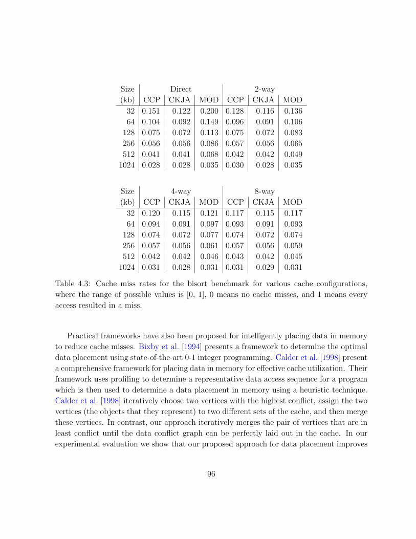
Size Direct 2-way

(kb) CCP CKJA MOD CCP CKJA MOD

32 0.151 0.122 0.200 0.128 0.116 0.136

64 0.104 0.092 0.149 0.096 0.091 0.106

128 0.075 0.072 0.113 0.075 0.072 0.083

256 0.056 0.056 0.086 0.057 0.056 0.065

512 0.041 0.041 0.068 0.042 0.042 0.049

1024 0.028 0.028 0.035 0.030 0.028 0.035

Size 4-way 8-way

(kb) CCP CKJA MOD CCP CKJA MOD

32 0.120 0.115 0.121 0.117 0.115 0.117

64 0.094 0.091 0.097 0.093 0.091 0.093

128 0.074 0.072 0.077 0.074 0.072 0.074

256 0.057 0.056 0.061 0.057 0.056 0.059

512 0.042 0.042 0.046 0.043 0.042 0.045

1024 0.031 0.028 0.031 0.031 0.029 0.031

Table 4.3: Cache miss rates for the bisort benchmark for various cache configurations,

where the range of possible values is [0, 1], 0 means no cache misses, and 1 means every

access resulted in a miss.

Practical frameworks have also been proposed for intelligently placing data in memory

to reduce cache misses. Bixby et al. [1994] presents a framework to determine the optimal

data placement using state-of-the-art 0-1 integer programming. Calder et al. [1998] present

a comprehensive framework for placing data in memory for effective cache utilization. Their

framework uses profiling to determine a representative data access sequence for a program

which is then used to determine a data placement in memory using a heuristic technique.

Calder et al. [1998] iteratively choose two vertices with the highest conflict, assign the two

vertices (the objects that they represent) to two different sets of the cache, and then merge

these vertices. In contrast, our approach iteratively merges the pair of vertices that are in

least conflict until the data conflict graph can be perfectly laid out in the cache. In our

experimental evaluation we show that our proposed approach for data placement improves

96

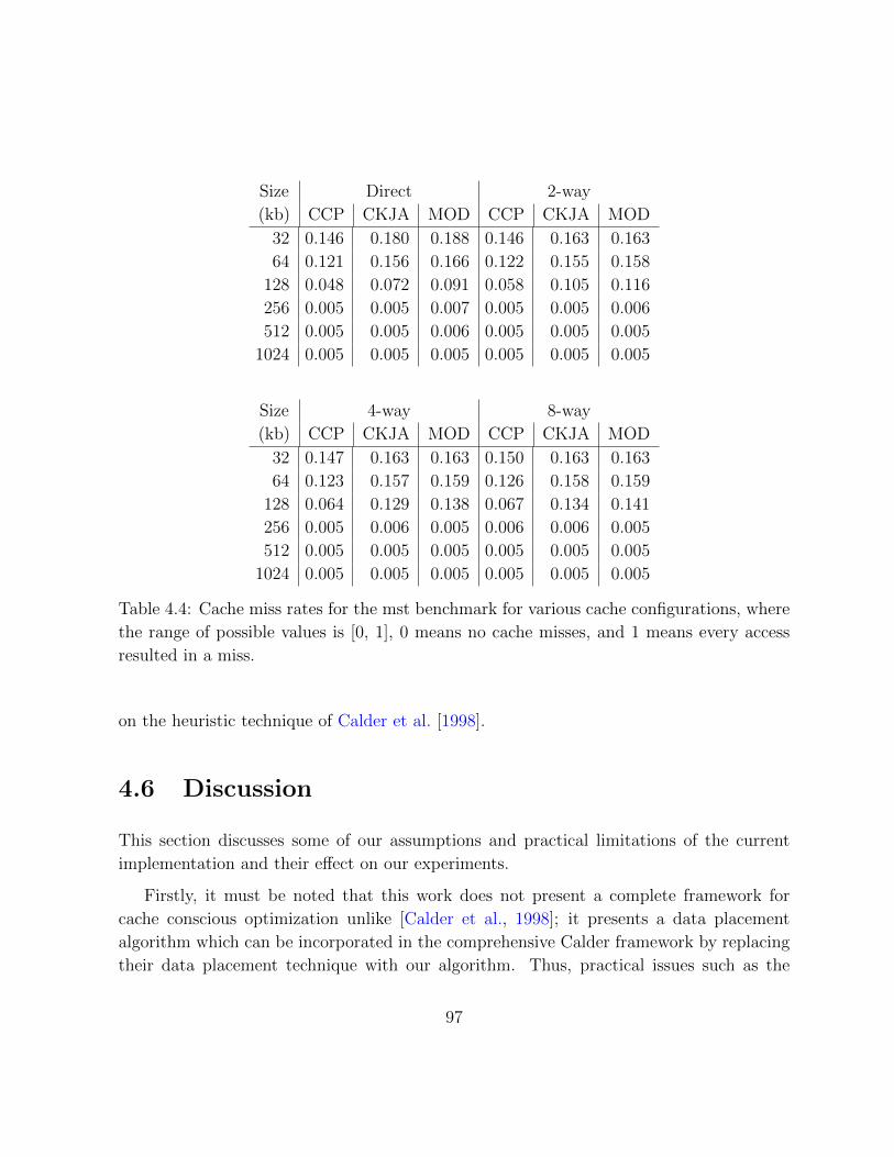
Size Direct 2-way

(kb) CCP CKJA MOD CCP CKJA MOD

32 0.146 0.180 0.188 0.146 0.163 0.163

64 0.121 0.156 0.166 0.122 0.155 0.158

128 0.048 0.072 0.091 0.058 0.105 0.116

256 0.005 0.005 0.007 0.005 0.005 0.006

512 0.005 0.005 0.006 0.005 0.005 0.005

1024 0.005 0.005 0.005 0.005 0.005 0.005

Size 4-way 8-way

(kb) CCP CKJA MOD CCP CKJA MOD

32 0.147 0.163 0.163 0.150 0.163 0.163

64 0.123 0.157 0.159 0.126 0.158 0.159

128 0.064 0.129 0.138 0.067 0.134 0.141

256 0.005 0.006 0.005 0.006 0.006 0.005

512 0.005 0.005 0.005 0.005 0.005 0.005

1024 0.005 0.005 0.005 0.005 0.005 0.005

Table 4.4: Cache miss rates for the mst benchmark for various cache configurations, where

the range of possible values is [0, 1], 0 means no cache misses, and 1 means every access

resulted in a miss.

on the heuristic technique of Calder et al. [1998].

4.6 Discussion

This section discusses some of our assumptions and practical limitations of the current

implementation and their effect on our experiments.

Firstly, it must be noted that this work does not present a complete framework for

cache conscious optimization unlike [Calder et al., 1998]; it presents a data placement

algorithm which can be incorporated in the comprehensive Calder framework by replacing

their data placement technique with our algorithm. Thus, practical issues such as the

97

distinction between stack and heap objects, and handling unknown objects which do not

appear in the profile have been discussed thoroughly by [Calder et al., 1998]. In future

work we will address some of these issues by creating the conflict graph from a small set of

data access profiles for each program and reserving a small number of sets in the cache to

handle objects for which a reasonable placement cannot be determined from the training

profiles. This would allow us to test our algorithm for arbitrary data access sequences for

a program once it has been profiled.

Secondly, the assumption that all objects are of the same size and fit a single cache

block does not hold true for most programs. This assumption does have an impact on

the evaluation of our approach, but does not affect the theoretical results presented in

this chapter. In a complete evaluation framework this assumption can be relaxed by

integrating existing split and merge techniques such as the ones given in [Chilimbi et al.,

1999a][Chilimbi et al., 1999b][Ding and Zhong, 2003] in order to improve the utilization

of cache blocks by coalescing conflicting objects or splitting large objects and regroup

conflicting fields. Since objects rarely fit a single block in the cache, coalescing and splitting

of objects is expected to dramatically reduce the size of the data conflict graph and hence

the runtime of the algorithm in practice.

Lastly, our approach does not cleanly address contiguous memory structures such as

arrays. We assume that each element of the array is an independent object which can be

mapped to any set in the cache. However, in reality, such an implementation would require

hardware support using mapping tables to map array elements to cache sets. Software

solutions may include introducing an additional level of indirection for array elements

based on the indices but may result in eliminating all performance gains achieved through

data placement. In order to extend the current solution we propose to handle array objects

as contiguous chunks of memory in future work.

In this work we highlight some of the theoretical issues related to cache-conscious

data placement. Although we acknowledge that more work needs to be done to make

our approach of practical interest, it contributes to our understanding of cache conscious

optimizations and allows us to appreciate the difficulty of the problem.

98

4.7 Summary

This study highlights the theoretical aspects of cache conscious data placement of objects

in memory. Cache conscious placement of data in memory is known to be intractable in

the worst-case, both to solve exactly and to approximate within reasonable bounds. The

main theoretical contribution of this chapter is the classification of data conflict graph as

an interval graph. This classification allows graph-theoretic results for interval graphs to be

applied to conflict graphs and to solve a special case of the cache conscious data placement

problem. We also present a cache conscious placement algorithm for finding a layout of the

objects in memory that is optimal if there exists a placement with no conflict misses. Fur-

ther, graph-theoretic techniques are used to heuristically reduce larger instances until the

optimization results can be applied. In summary, our graph-theoretic algorithm performed

well on most instances. On a variety of realistic cache configurations and benchmarks, our

approach improves the cache hit ratio over the best previous techniques by 9% to 21% on

average.

99

Chapter 5

Conclusions and Future Work

This thesis examined three different compiler optimization problems. The first problem

was spatial and temporal scheduling for clustered architectures and we presented a solution

using decomposition techniques and constraint programming. The second problem was the

selection of architecture specific instructions in the compiler code generation phase. A con-

straint programming approach was proposed to identify the exact solution for transforming

compiler specific code to machine instructions. The third problem was the offline version

of cache optimization and was solved using graph theoretic optimization techniques.

In further detail, for the first problem we extended and improved upon a constraint

programming solution for temporal scheduling. Specifically, instructions are assigned to

different clusters in addition to assigning them to clock cycles. We applied problem decom-

position techniques to solve spatial and temporal scheduling in an integrated manner and

to scale the solution to large problem sizes. The effect of different hardware parameters

has been analyzed—such as the number of clusters, issue-width and inter-cluster communi-

cation cost—on application performance. The inclusion of symmetry breaking constraints

and the detection of connected structures reduces the scheduling time considerably. The

results of the experiments show that the constraint programming approach is able to im-

prove the schedule quality by up to 26% on average. The algorithm successfully solved

more than 80% of the benchmarks optimally with a few additional hours of compile time.

The second problem addressed in this thesis is instruction selection in the code gener-

ation phase of the compiler. Instruction selection is an interesting problem as it has an

impact on the other phases of code generation including instruction scheduling and register

100

allocation. To solve the instruction selection problem, we again employed techniques from

constraint modeling along with constraint propagation to improve the quality of compiled

code and scale the solution to large problem sizes. The experimental evaluation that uses

an implementation of the constraint satisfaction problem integrated into the LLVM com-

piler, shows that the exact algorithm can solve over 95% of all benchmarks. However,

the resultant performance improvements in selection cost as compared to the hand-tuned

LLVM selector are less than 4% on average. The algorithm results in an improvement of

about 1% in terms of code size.

The third problem addressed in this thesis is that of offline cache optimization. Using

a graph theoretic framework, we showed that certain instances can be identified such that

the generally hard cache optimization problem can be solved accurately and efficiently.

For such instances, we propose a cache placement algorithm that is optimal and conflict

misses can be avoided altogether. We also propose a second algorithm that employs graph

theoretic techniques to solve the memory data layout problem for larger instances where the

size of the cache forces conflict misses. On a variety of benchmark instances the algorithm

has been shown to improve cache hit rates by up to 21% on average.

All together, our results show that exact solutions for difficult combinatorial problems

in compilers can be found. Here, exact solutions were obtained through the application

and development of theoretical and constraint programming techniques. These problem-

solving techniques are effective for compiler optimization in that they lead to significant

improvements.

For future work, several improvements can be identified to improve the current state

of the solutions proposed in this thesis. In regard to the spatial and temporal scheduling

problem, it can be further improved upon by identifying implied constraints and improving

the detection mechanism for complex connected structures that are not chains. The in-

struction selection problem can be extended to integrate other compiler optimizations. For

example, our experimental results suggest that register allocation can have a significant

impact on the code size. Hence, a combined solution for instruction selection, instruction

scheduling and register allocation could be a topic for future work. The offline problem of

cache optimization can be extended in several ways. One avenue for future work that our

current solution and previous work does not adequately address is the issue of contiguous

memory structures like arrays. A second, potentially promising, avenue for future work

is the investigation of whether structure splitting and coalescing techniques can be used

101

within our proposals to significantly reduce the size of the conflict graph. Smaller problem

instances could then be solved using optimal techniques to find a more accurate placement

of data in memory.

102

APPENDICES

103

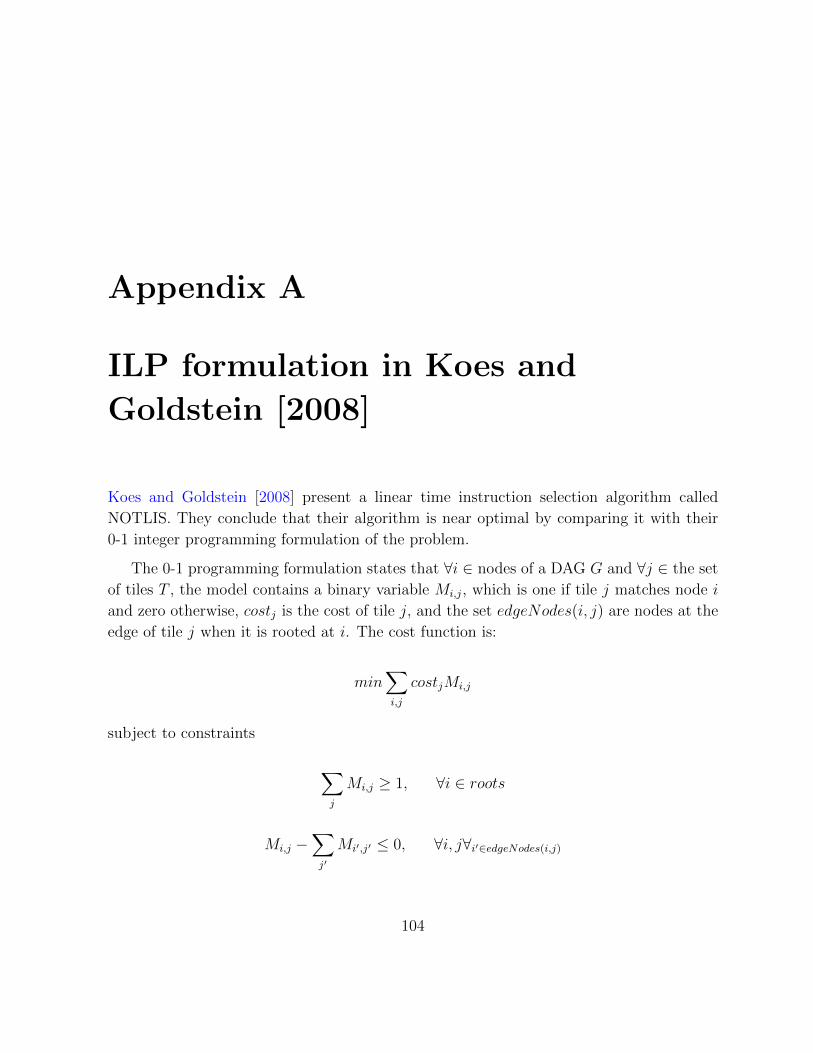
Appendix A

ILP formulation in Koes and

Goldstein [2008]

Koes and Goldstein [2008] present a linear time instruction selection algorithm called

NOTLIS. They conclude that their algorithm is near optimal by comparing it with their

0-1 integer programming formulation of the problem.

The 0-1 programming formulation states that ∀i ∈ nodes of a DAG G and ∀j ∈ the set

of tiles T , the model contains a binary variable Mi,j, which is one if tile j matches node i

and zero otherwise, costj is the cost of tile j, and the set edgeNodes(i, j) are nodes at the

edge of tile j when it is rooted at i. The cost function is:

min∑i,j

costjMi,j

subject to constraints

∑j

Mi,j ≥ 1, ∀i ∈ roots

Mi,j −∑j′

Mi′,j′ ≤ 0, ∀i, j∀i′∈edgeNodes(i,j)

104

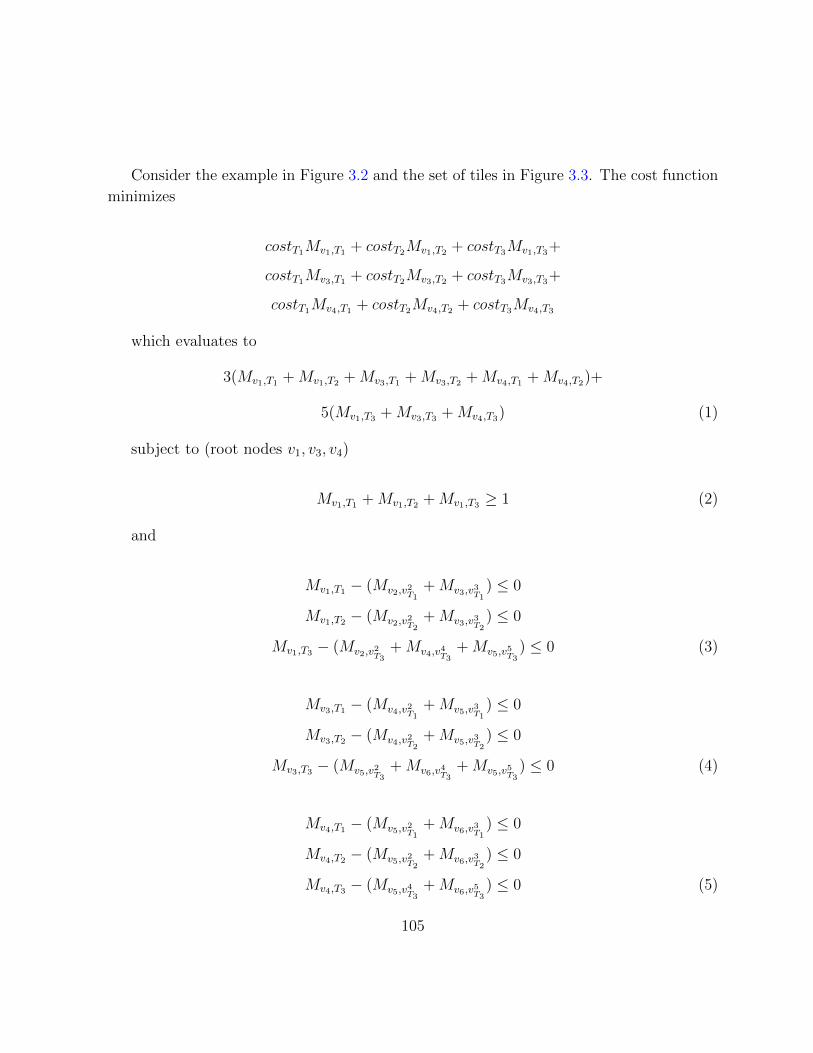
Consider the example in Figure 3.2 and the set of tiles in Figure 3.3. The cost function

minimizes

costT1Mv1,T1 + costT2Mv1,T2 + costT3Mv1,T3+

costT1Mv3,T1 + costT2Mv3,T2 + costT3Mv3,T3+

costT1Mv4,T1 + costT2Mv4,T2 + costT3Mv4,T3

which evaluates to

3(Mv1,T1 +Mv1,T2 +Mv3,T1 +Mv3,T2 +Mv4,T1 +Mv4,T2)+

5(Mv1,T3 +Mv3,T3 +Mv4,T3) (1)

subject to (root nodes v1, v3, v4)

Mv1,T1 +Mv1,T2 +Mv1,T3 ≥ 1 (2)

and

Mv1,T1 − (Mv2,v2T1+Mv3,v3T1

) ≤ 0

Mv1,T2 − (Mv2,v2T2+Mv3,v3T2

) ≤ 0

Mv1,T3 − (Mv2,v2T3+Mv4,v4T3

+Mv5,v5T3) ≤ 0 (3)

Mv3,T1 − (Mv4,v2T1+Mv5,v3T1

) ≤ 0

Mv3,T2 − (Mv4,v2T2+Mv5,v3T2

) ≤ 0

Mv3,T3 − (Mv5,v2T3+Mv6,v4T3

+Mv5,v5T3) ≤ 0 (4)

Mv4,T1 − (Mv5,v2T1+Mv6,v3T1

) ≤ 0

Mv4,T2 − (Mv5,v2T2+Mv6,v3T2

) ≤ 0

Mv4,T3 − (Mv5,v4T3+Mv6,v5T3

) ≤ 0 (5)

105

Note that matching v4 with T3 is not possible as the number of edge nodes in T3 are

more than what can be matched when T3 is rooted at v4. So in the last constraint Mv4,T3

is only matching the internal operation in T3 with v4.

As is evident from equation (1), the cost is between 9 and 15 given only constraints in

equations (2). Constraints (3) to (5) attempt to match the tiles but only are able to match

the structure and not the types and can possibly result in a flawed solution.

The flaw in the formulation is that the Mi,j are decision variables assigned values by

the solver which can assign Mv1,T1 = 1 as well as Mv1,T2 = 1 and the constraints would

still hold. This is because the constraints do not handle the mismatch of opcodes or types.

Thus, the 0-1 programming model presented is incomplete and Mv1,T1 = 1, Mv3,T3 = 1 and

Mv4,T3 = 1 would be regarded as a correct solution by the solver. In this instance its cost

is equal to the correct optimal solution, but the resultant tiling is incorrect.

106

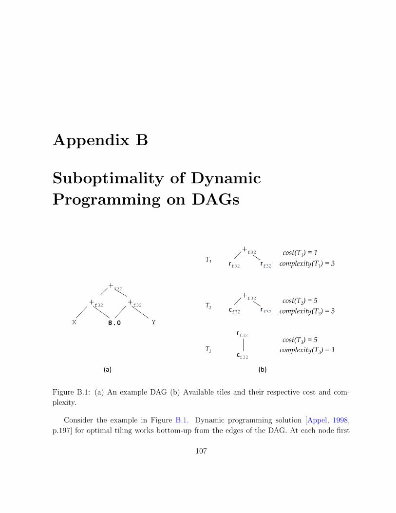
Appendix B

Suboptimality of Dynamic

Programming on DAGs

Figure B.1: (a) An example DAG (b) Available tiles and their respective cost and com-

plexity.

Consider the example in Figure B.1. Dynamic programming solution [Appel, 1998,

p.197] for optimal tiling works bottom-up from the edges of the DAG. At each node first

107

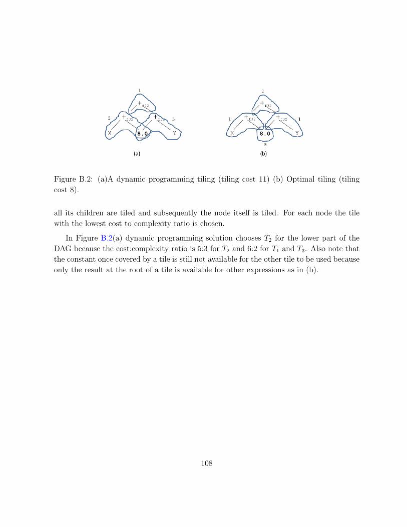
Figure B.2: (a)A dynamic programming tiling (tiling cost 11) (b) Optimal tiling (tiling

cost 8).

all its children are tiled and subsequently the node itself is tiled. For each node the tile

with the lowest cost to complexity ratio is chosen.

In Figure B.2(a) dynamic programming solution chooses T2 for the lower part of the

DAG because the cost:complexity ratio is 5:3 for T2 and 6:2 for T1 and T3. Also note that

the constant once covered by a tile is still not available for the other tile to be used because

only the result at the root of a tile is available for other expressions as in (b).

108

References

Aggarwal, A., and Franklin, M. 2005. Scalablility aspects of instruction distribu-

tion algorithms for clustered processors. IEEE Transactions on Parallel and Distributed

Systems, 16, 10, 944–955.

Aleta, A., Codina, J. M., Sanchez, J., Gonzalez, A., and Kaeli, D. 2009. AG-

AMOS: A graph-based approach to modulo scheduling for clustered microarchitectures.

IEEE Transactions on Computers, 58, 6, 770–783.

Amarasinghe, S., Karger, D. R., Lee, W., and Mirrokni, V. S. 2002. A theoreti-

cal and practical approach to instruction scheduling on spatial architectures. Laboratory

of Computer Science, MIT, Tech. Report.

Andreev, K., and Racke, H. 2004. Balanced graph partitioning. In Proceedings of

the Sixteenth Annual ACM Symposium on Parallelism in Algorithms and Architectures,

120–124.

Appel, A. W. 1998. Modern Compiler Implementation in C. Cambridge University Press.

1998.

ARM, The architecture for the digital world. http://www.arm.com. Retrieved June, 2011.

Baek, W., and Chilimbi, T. M. 2010. Green: a framework for supporting energy-

conscious programming using controlled approximation. In Proceedings of the 2010 ACM

SIGPLAN Conference on Programming Language Design and Implementation (PLDI

’10), 198–209.

Bashford, S., and Leupers, R. 1999. Phase-coupled mapping of data flow graphs to

irregular data paths. In Design Automation for Embedded Systems 4, 119–165.

109

Bashford, S., and Leupers, R. 1999. Constraint driven code selection for fixed-point

DSPs. In 36th ACM Design Automation Conference 4, 119–165.

Bednarski, A. and Kessler, C. W. 2006. Optimal integrated VLIW code generation

with integer linear programming. In Euro-Par ’06, 461–472.

Beg, M. 2010. Instruction scheduling for multi-cores. Student Research Competition at

the Conference on Programming Language Design and Implementation.

Beg, M., and van Beek, P. 2011. A constraint programming approach to instruc-

tion assignment. The 15th Annual Workshop on the Interaction between Compilers and

Computer Architecture (INTERACT’15).

Beg, M., and van Beek, P. 2013. A constraint programming approach for integrated

spatial and temporal scheduling for clustered architectures. ACM Transactions on Em-

bedded Computing Systems, To appear.

Beg, M. and van Beek, P. 2010. A graph theoretic approach to cache-conscious place-

ment of data for direct mapped caches. In Proceedings of the 2010 International Sym-

posium on Memory Management (ISMM ’10), 113–120.

Benders, J. F. 1962. Partitioning procedures for solving mixed-variables programming

problems. Numerische Mathematik 4, 238–252.

Bixby, R. E., Kennedy, K., and Kremer, U. 1994. Automatic data layout using

0-1 integer programming. In Proceedings of the IFIP WG10.3 Working Conference on

Parallel Architectures and Compilation Techniques (PACT ’94), 111–122.

Bjerregaard, T., and Mahadevan, S. 2006. A survey of research and practices of

network-on-chip. ACM Computing Surveys, 38, 1, 1–51.

Blainey, R. J. 1994. Instruction scheduling in the TOBEY compiler. IBM J. Res. De-

velop., 38, 5, 577–593.

Buchwald, S. and Zwinkau, A. 2010. Instruction selection by graph transformation.

In Proceedings of the 2010 International Conference on Compilers, Architectures and

Synthesis for Embedded Systems (CASES ’10), 31–40.

110

Calder, B., Krintz, C., John, S., and Austin, T. 1998. Cache-conscious data place-

ment. In Proceedings of the Eighth International Conference on Architectural Support

for Programming Languages and Operating Systems (ASPLOS-VIII), 139–149.

Cantin, J. F. and Hill, M. D. 2001. Cache performance for selected SPEC CPU 2000

benchmarks. http://research.cs.wisc.edu/multifacet/misc/spec2000cache-data

CEVA. CEVA-X Architecture CEVA-X 1620/1622. http://www.ceva-dsp.com. Retrieved

December, 2012.

Chakrapani, L., Gyllenhaal, J., Hwu, W.-M., Mahlke, S. A., Palem, K. V.

and Rabbah, R. M. 2005. Trimaran: An infrastructure for research in instruction-level

parallelism. Proceedings of Languages and Compilers for High Performance Computing,

32–41.

Chilimbi, T. M. and Larus, J. R. 1998. Using generational garbage collection to imple-

ment cache-conscious data placement. In Proceedings of the 1st International Symposium

on Memory Management (ISMM ’98), 37–48.

Chilimbi, T. M., Davidson, B., and Larus, J. R. 1999. Cache-conscious structure

definition. In Proceedings of the ACM SIGPLAN 1999 Conference on Programming

Language Design and Implementation (PLDI ’99), 13–24.

Chilimbi, T. M., Hill, M. D., and Larus, J. R. 1999. Cache-conscious structure lay-

out. In Proceedings of the ACM SIGPLAN 1999 Conference on Programming Language

Design and Implementation (PLDI ’99), 1–12.

Chilimbi, T. M. 2001. Efficient representations and abstractions for quantifying and

exploiting data reference locality. In Proceedings of the ACM SIGPLAN 2001 Conference

on Programming Language Design and Implementation (PLDI ’01), 191–202.

Chilimbi, T. M. and Hirzel, M. 2002. Dynamic hot data stream prefetching for

general-purpose programs. In Proceedings of the ACM SIGPLAN 2002 Conference on

Programming Language Design and Implementation (PLDI ’02), 199–209.

Chilimbi, T. M. and Shaham, R. 2006. Cache-Conscious Coallocation of Hot Data

Streams. In Proceedings of the ACM SIGPLAN 2006 Conference on Programming Lan-

guage Design and Implementation (PLDI ’06), 252–263.

111

Chu, M., Fan, K., and Mahlke, S. 2003. Region-based hierarchical operation parti-

tioning for multicluster processors. In Proceedings of the ACM SIGPLAN 2003 Confer-

ence on Programming Language Design and Implementation (PLDI’03), 300–311.

Chu, M., and Mahlke, S. 2006. Compiler-directed data partitioning for multiclus-

ter processors. In Proceedings of the International Symposium on Code Generation and

Optimization (CGO’06), 208–220.

Chu, M., Ravindran, R., and Mahlke, S. 2007. Data access partitioning for

fine-grain parallelism on multicore architectures. In Proceedings of the 40th Annual

IEEE/ACM International Symposium on Microarchitecture (Micro’07), 369–380.

Chung, Y. C., Liu, C. C., and Liu, J. S. 1995. Applications and performance anal-

ysis of an optimization approach for list scheduling algorithms on distributed memory

multiprocessors. Journal of Information Science and Engineering, 11, 2, 155–181.

Codina, J. M., Sanchez, J. F, and Gonzalez, A. 2001. A unified modulo schedul-

ing and register allocation technique for clustered processors. In Proceedings of the

10th International Conference on Parallel Architectures and Compilation Techniques

(PACT’01), 175–184.

Dantzig, G. B., and Wolfe, P. 1960. Decomposition principle for linear programs.

Operations Research, 8, 101–111.

Deville, Y. Dooms, G. Zampelli, S. and Dupont, P. 2005. CP(Graph+Map) for

approximate graph matching. In 1st International Workshop on Constraint Programming

Beyond Finite Integer Domains, at CP2005, 31–47.

Ding, C. and Kennedy, K. 1999. Improving cache performance in dynamic applica-

tions through data and computation reorganization at run time. In Proceedings of the

ACM SIGPLAN 1999 Conference on Programming Language Design and Implementa-

tion (PLDI ’99), 229–241.

Ding, C. and Zhong, Y. 2003. Predicting whole-program locality through reuse dis-

tance analysis. In Proceedings of the ACM SIGPLAN 2003 Conference on Programming

Language Design and Implementation (PLDI ’03), 245–257.

112

Dooms, G. Deville, Y. and Dupont, P. 2005. CP(Graph): Introducing a graph com-

putation domain in constraint programming. In Principles and Practice of Constraint

Programming (CP 2005), 211–225.

Ebner, D., Brandner, F., Scholz, B., Krall, A., Wiedermann, P., and

Kadlec, A. 2008. Generalized instruction selection using SSA-graphs. In Proceed-

ings of the 2008 ACM SIGPLAN-SIGBED Conference on Languages, Compilers, and

Tools for Embedded Systems (LCTES ’08), 31–40.

Eckstein, E., Konig, O., and Scholz, B. 2003. Code instruction selection based on

SSA-graphs. In Proceedings of the Workshop on Software and Compilers for Embedded

Systems (SCOPES ’03), 49–65.

Ellis, J. R. 1986. Bulldog: A compiler for VLSI architectures. MIT Press.

Eriksson, M. V. and Kessler, C. W. 2009. Integrated modulo scheduling for clus-

tered VLIW architectures. In Proceedings of the 4th International Conference on High

Performance Embedded Architectures and Compilers (HiPEAC’09), 65–79.

Eriksson, M. V. and Kessler, C. W. 2008. Integrated modulo scheduling for clus-

tered VLIW architectures. In Proceedings of the 4th International Conference on High

Performance Embedded Architectures and Compilers (HiPEAC ’09), 65–79.

Eriksson, M. V.,Skoog, O., and Kessler, C. W. 2008. Optimal vs. heuristic in-

tegrated code generation for clustered VLIW architectures. In Proceedings of the 11th

International Workshop on Software and Compilers for Embedded Systems (SCOPES

’08), 11–20.

Ertl, M. A. 1999. Optimal code selection in DAGs. In Proceedings of the 26th ACM

SIGPLAN-SIGACT Symposium on Principles of Programming Languages (POPL ’99),

242–249.

Faraboschi, P., Desoli, G., and Fisher, J. A. 1998. Clustered instruction-level

parallel processors. HP Labs Technical Report HPL-98-204, 1–29.

Fisher, J. A., Faraboschi, P., and Young, C. 2005. Embedded Computing: A VLIW

Approach to Architecture, Compilers, and Tools. Morgan Kaufmann, Menlo Park, USA.

113

Fraser, C. W., Henry, R. R., and Proebsting, T. A. 2008. BURG: fast optimal

instruction selection and tree parsing. In SIGPLAN Notices, 27, 4:68–76.

Golumbic, M. C. 2004. Algorithmic Graph Theory and Perfect Graphs (Annals of Dis-

crete Mathematics, Vol 57). North-Holland Publishing Co., Amsterdam, The Nether-

lands.

Gu, X., Christopher, I., Bai, T., Zhang, C., and Ding, C. 2009. A component

model of spatial locality. In Proceedings of the 2009 International Symposium on Memory

Management (ISMM ’09), 99–108.

Hack, S. and Goos, G. 2006. Optimal register allocation for SSA-form programs in

polynomial time. Information Processing Letters 98, 150–155.

Heffernan, M., and Wilken, K. 2005. Data-dependency graph transformations for

instruction scheduling. Journal of Scheduling, 8, 427–451.

Heffernan, M., Wilken, K., and Shobaki, G. 2006. Data-dependency graph trans-

formations for superblock scheduling. In Proceedings of the 39th Annual IEEE/ACM

International Symposium on Microarchitecture (Micro’06), 77–88.

Hendrickson, B., and Leland, R. 1995. A multilevel algorithm for partitioning

graphs. In Proceedings of the 1995 ACM/IEEE Conference on Supercomputing (Super-

computing’95), 28.

Hennessy, J. L. and Patterson, D. A. 2004. Computer Architecture; A Quantitative

Approach 4th Ed. Morgan Kaufmann, San Francisco, USA.

Hoffmann, H., Sidiroglou, S., Carbin, M., Misailovic, S., Agarwal, A., and

Rinard, M. 2011. Dynamic knobs for responsive power-aware computing. In Proceed-

ings of the sixteenth International Conference on Architectural Support for Programming

Languages and Operating Systems (ASPLOS ’11), 199–212.

Hoxey, S., Karim, F., Hay, B., and Warren, H. 1996. The PowerPC Compiler

Writers Guide, Warthman Associates.

Jin, G., Mellor-Crummey, J., and Fowler, R. 2001. Increasing temporal locality

with skewing and recursive blocking. In Proceedings of the 2001 ACM/IEEE Conference

on Supercomputing (Supercomputing ’01), 43–43.

114

Jula, A. and Rauchwerger, L. 2009. Two memory allocators that use hints to improve

locality. In Proceedings of the 2009 International Symposium on Memory Management

(ISMM ’09), 109–118.

Karypis, G. and Kumar, V. 1998. A fast and high quality multilevel scheme for

partitioning irregular graphs. SIAM Journal on Scientific Computing, 20, 1, 359–392.

Kessler, C. W. and Bednarski, A. 2006. Optimal integrated code generation for

VLIW architectures. Concurrency and Computation: Practice and Experience, 18, 11,

1353–1390.

Kessler, C., and Bednarski, A. 2001. A Dynamic Programming Approach to Opti-

mal Integrated Code Generation. In Proceedings of the 2001 ACM SIGPLAN-SIGBED

Conference on Languages, Compilers, and Tools for Embedded Systems (LCTES ’01),

163–174.

Kessler, C., and Bednarski, A. 2002. Optimal integrated code generation for clus-

tered VLIW architectures. In Proceedings of the joint Conference on Languages, Com-

pilers and Tools for Embedded Systems: Software and Compilers for Embedded Systems

(LCTES/SCOPES ’02), 102–111.

Kessler, C., and Bendnarski, A. 2006. Optimal integrated code generation for VLIW

architectures. In Concurrency and Computation: Practice and Experience, John Wiley

& Sons, Ltd. 18, 11:1353–1390.

von Koch, T. E., Bhm, I., and Franke, B. 2010. Integrated instruction selection and

register allocation for compact code generation exploiting freeform mixing of 16- and

32-bit instructions. Proceedings of the 8th annual IEEE/ACM international symposium

on Code Generation and Optimization (CGO ’10).

Koes, D. R., and Goldstein, S. C. 2008. Near-optimal instruction selection on dags In

Proceedings of the 6th annual IEEE/ACM International Symposium on Code Generation

and Optimization (CGO ’08), 45–54.

Ulrich Kremer 1997. Optimal and near-optimal solutions for hard compilation prob-

lems. In Parallel Processing Letters 7, 4:371–378.

115

Lapinskii, V. S., Jacome, M. F., and De Veciana, G. A. 2002. Cluster assign-

ment for high-performance embedded VLIW processors. ACM Transactions on Design

Automation of Electronic Systems, 7, 430–454.

Lattner, C., and Adve, V. 2004. LLVM: A compilation framework for lifelong program

analysis & transformation. In Proceedings of the International Symposium on Code

generation and Optimization (CGO ’04), 75–86.

Lattner, C. and Adve, V. 2005. Automatic pool allocation: improving performance by

controlling data structure layout in the heap. In Proceedings of the 2005 ACM SIGPLAN

Conference on Programming Language Design and Implementation (PLDI ’05), 129–142.

Lee, W., Barua, R., Frank, M., Srikrishna, D., Babb, J., Sarkar, V., and

Amarasinghe, S. 1998. Space-time scheduling of instruction-level parallelism on a

RAW machine. In Proceedings of the Eighth International Conference on Architectural

Support for Programming Languages and Operating Systems (ASPLOS-VIII), 46–57.

Lee, W., Puppin, D., Swenson, S., and Amarasinghe, S. 2002. Convergent schedul-

ing. In Proceedings of the 35th annual ACM/IEEE International Symposium on Microar-

chitecture (Micro’35), 111–122.

Leupers, R. 2000. Instruction Scheduling for Clustered VLIW DSPs. In Proceedings of

IEEE International Conference on Parallel Architectures and Compilation Techniques

(PACT’00), 291–300.

Leupers, R., and Bashford, S. 2000. Graph-based code selection techniques for em-

bedded processors. In ACM Transactions on Design Automation of Electronic Systems

(TODEAS) 5, 4:794–814.

Liao, S. Y., Devadas, S., Keutzer, K., and Tjiang, S. W. K. 2008. Instruction

selection using binate covering for code size optimization. In Proceedings of the 1995

IEEE/ACM International Conference on Computer-Aided Design (ICCAD ’95), 393–

399.

Luo, C., Bai, Y., Xu, C., and Zhang, L. 2009. FCCM: A novel inter-core commu-

nication mechanism in multi-core platform. In Proceedings of International Conference

on Science and Engineering, 215–218.

116

Malik, A. M., McInnes, J., and van Beek, P. 2008. Optimal basic block instruc-

tion scheduling for multiple-issue processors using constraint programming. International

Journal on Artificial Intelligence Tools, 17, 1, 37–54.

Malik, A. M., Chase, M., Russell, T., and van Beek, P. 2008. An application of

constraint programming to superblock instruction scheduling. In Proceedings of the Four-

teenth International Conference on Principles and Practice of Constraint Programming

(CP’08), 97–111.

Lee, C., Potkonjak, M. and Manginoe-Smith, W. 1997. MediaBench: A tool for

evaluating and synthesizing multimedia and communications. Proceedings of the 30th

Annual IEEE/ACM International Symposium on Microarchitecture (Micro-30), 330–335.

Guthaus, M. R., Ringenberg, J. S., Ernst, D., Austin, T. M., Mudge, T.,

and Brown, R. B. 2001. MiBench: A free, commercially representative embedded

benchmark suite. Proceedings of the IEEE International Workshop on Workload Char-

acterization (WWC-4), 3–14.

Naik, M., and Palsberg, J. 2004. Compiling with code-size constraints. In ACM

Transactions on Embedded Computing Systems (TECS) 3, 1:163–181.

Nagpal, R., and Srikant, Y. N. 2004. Integrated temporal and spatial scheduling

for extended operand clustered VLIW processors. Conference on Computing Frontiers,

457–470.

Nagpal, R., and Srikant, Y. N. 2011. Compiler-assisted power optimization for

clustered VLIW architectures. In Parallel Computing, 37, 1:42–59.

Nagpal, R., and Srikant, Y. N. 2008. Pragmatic integrated scheduling for clustered

VLIW architectures. Software Practice and Experience, 38, 227–257.

Ramsey, N., and Dias, J. 2011. Resourceable, retargetable, modular instruction selec-

tion using a machine-independent, type-based tiling of low-level intermediate code. In

Proceedings of the 38th annual ACM SIGPLAN-SIGACT Symposium on Principles of

Programming Languages (POPL ’11). 575–586.

Nystrom, E., and Eichenberger, A. E. 1998. Effective cluster assignment for modulo

scheduling. In Proceedings of the 31st Annual ACM/IEEE International Symposium on

Microarchitecture (Micro’98).

117

Owens, J. D., Dally, W. J., Ho, R., Jayasimha, D. N., Keckler, S. W. and

Peh, L. 2007. Research challenges for on-chip interconnection networks. IEEE Micro,

27, 5, 96–108.

Parcerisa, J-M., Sahuqillo, J., Gonzalez, A., and Duato, J. 2002. Efficient

interconnects for clustered microarchitectures. In Proceedings of the 2002 International

Conference on Parallel Architectures and Compilation Techniques (PACT’02), 291–300.

Proebsting, T. 1998. Least-cost instruction selection in DAGs is NP-

complete. In Privately Published Online, http://research.microsoft.com/en-

us/um/people/toddpro/papers/proof.htm.

Petrank, E. and Rawitz, D. 2002. The hardness of cache conscious data placement.

In Proceedings of the 29th ACM SIGPLAN-SIGACT Symposium on Principles of Pro-

gramming Languages (POPL ’02), 101–112.

Petrank, E. and Rawitz, D. 2005. The hardness of cache conscious data placement.

Nordic Journal of Computing 12, 275–307.

Prokopski, G. B. and Verbrugge, C. 2008. Analyzing the performance of code-

copying virtual machines. In Proceedings of the 23rd ACM SIGPLAN Conference on

Object-Oriented Programming Systems Languages and Applications (OOPSLA ’08), 403–

422.

Rich, K. and Farrens, M. 2000. Code partitioning in decoupled compilers. In Pro-

ceedings from the 6th International Euro-Par Conference on Parallel Processing (Euro-

Par’00), 1008–1017.

Russell, T., Malik, A., Chase, M., and van Beek, P. 2009. Learning heuristics for

the superblock instruction scheduling problem. IEEE Transactions on Knowledge and

Data Engineering, 21, 10, 1489–1502.

Rossi, F., van Beek, P., and Walsh, T. (Ed). 2006. Handbook of Constraint Pro-

gramming. Elsevier.

Sanchez, J., and Gonzalez, A. 2000. Modulo scheduling for a fully-distributed clus-

tered VLIW architecture. In Proceedings of the 33th Annual IEEE/ACM International

Symposium on Microarchitecture (Micro’00), 124–133

118

Sanchez, J., and Gonzalez, A. 2000. Instruction scheduling for clustered VLIW

architectures. In Proceedings of the 13th International Symposium on System Synthesis

(ISSS’00), 41–46.

Schafer, S., and Scholz, B. 2007. Optimal chain rule placement for instruction

selection based on SSA graphs. In Proceedings of the 10th international workshop on

Software & compilers for embedded systems (SCOPES ’07), 91–100.

Shen, X., Shaw, J., Meeker, B., and Ding, C. 2007. Locality approximation us-

ing time. In Proceedings of the 34th Annual ACM SIGPLAN-SIGACT Symposium on

Principles of Programming Languages (POPL ’07), 55–61.

Shobaki, G. and Wilken, K. 2004. Optimal superblock scheduling using enumeration.

In Proceedings of the 37th Annual IEEE/ACM International Symposium on Microarchi-

tecture (Micro’04), 283–293.

Terechko, A. S., and Corporaal, H. 2007. Inter-cluster communication in VLIW

architectures. Transactions on Architecture and Code Optimization (TACO), 4, 2, 1–38.

Terechko, A. S. 2007. Clustered VLIW architectures: a quantitative approach. Doctoral

Thesis, Technischie Universiteit Eindhoven.

Texas Instruments. http://www.ti.com. Retrieved June, 2011.

Thabit, K. O. 1982. Cache management by the compiler. PhD thesis, Rice University,

Houston, USA.

Torczon, L., and Cooper, K. 2007. Engineering a compiler. Morgan Kaufmann

Publishers.

Rabbah, R. M., Bratt, I., Asanovic, K. and Agarwal, A. 2004. Versatility and

versabench: A new metric and a benchmark suite for flexible architectures. Computer

Science and Artifical Intelligence Laboratory, MIT, Tech. Report.

Wolf, M. E., Maydan, D. E., and Chen, D.-K. 1998. Combining loop transformations

considering caches and scheduling. International Journal of Parallel Programming 26,

479–503.

119

Zampelli, S., Deville, Y., and Dupont, P. 2005. Approximate Constrained Sub-

graph Matching. In Principles and Practice of Constraint Programming, Lecture Notes

in Computer Science (CP 2005), 832–836.

Zampelli, S., Deville, Y., and Dupont, P. 2005. Declarative Approximate Graph

Matching Using a Constraint Approach. In Second International Workshop on Con-

straint Propagation and Implementation, 109–124.

Zhang, C., Ding, C., Ogihara, M., Zhong, Y., and Wu, Y. 2006. A hierarchical

model of data locality. In Conference Record of the 33rd ACM SIGPLAN-SIGACT

Symposium on Principles of Programming Languages (POPL ’06), 16–29.

Zhong, Y. and Chang, W. 2008. Sampling-based program locality approximation. In

Proceedings of the 7th International Symposium on Memory Management (ISMM ’08),

91–100.

Zhong, Y., Shen, X., and Ding, C. 2009. Program locality analysis using reuse dis-

tance. ACM Transactions on Programming Languages and Systems (TOPLAS) 31, 20:1–

20:39.

120