Combinations of Local Search and Constraint...
124
Combinations of Local Search and Constraint Programming Masterclass on Hybrid Methods, Toulouse, 4-5 June 2018 Paul Shaw IBM Analytics, France Paul Shaw Combinations of Local Search and Constraint Programming
Transcript of Combinations of Local Search and Constraint...

Combinations of Local Search and ConstraintProgramming
Masterclass on Hybrid Methods, Toulouse, 4-5 June 2018
Paul Shaw
IBM Analytics, France
Paul Shaw Combinations of Local Search and Constraint Programming

Why?
Local SearchProvides good solutions quicklyGood for pure problems with few constraintsScales well
Constraint ProgrammingComplete, can provide proofsGood for problems with lots of constraints
Paul Shaw Combinations of Local Search and Constraint Programming

Source text
Constraint Programming and Local Search Hybrids in
Paul Shaw Combinations of Local Search and Constraint Programming

Outline
Constraint-based local searchLocal search on the decision pathExploring neighborhoods using CPLarge neighborhood searchLocal search for pruning and propagationLocal search and dominance
Paul Shaw Combinations of Local Search and Constraint Programming
Constraint-based LocalSearch
Paul Shaw Combinations of Local Search and Constraint Programming

Constraint-based Local Search
By “constraint-based local search”, I mean using local searchon CSP-type models. This type of approach was born in theearly 1990s. For example:
Min-conflicts (Minton et al., 1992)Breakout (Morris, 1993), GENET (Davenport et al. 1994)GSAT (Selman et al., 1992)
Paul Shaw Combinations of Local Search and Constraint Programming

Constraint-based Local Search
Min-conflicts
Paul Shaw Combinations of Local Search and Constraint Programming

Constraint-based Local Search
Min-conflicts
Of course, can fall foul of local minima.
A,B,C ∈ {0, 1}
A+B + C ≥ 1 A 6= C B 6= C
Start at A = 1, B = 0, C = 0(Only solution is A = 0, B = 0, C = 1)
Paul Shaw Combinations of Local Search and Constraint Programming

Constraint-based Local Search
Min-conflicts
Of course, can fall foul of local minima.
Paul Shaw Combinations of Local Search and Constraint Programming

Constraint-based Local Search
Min-conflicts
Of course, can fall foul of local minima.
GENET and “breakout” took the same approach:
- At a local minimum, increase the violation weights of theconstraints in conflict
Paul Shaw Combinations of Local Search and Constraint Programming

Constraint-based Local Search
GSAT
To fight against local minima:
- Makes a random move among the best- Restarts the search
Paul Shaw Combinations of Local Search and Constraint Programming

Constraint-based Local Search
Systems
The main CBLS systems are Localizer and COMET
They are toolkits which provide efficient primitives allowing auser to write a model and custom local search procedure.
Paul Shaw Combinations of Local Search and Constraint Programming
Constraint-based Local Search
Systems: Localizer
Localizer uses a declarative language to define move selectionrules.
Central to this is the idea of invariants and incrementality.
Invariants are efficiently and incrementally updated whendecision variables change their value.
No real concept of constraints or violation
Paul Shaw Combinations of Local Search and Constraint Programming

Constraint-based Local Search
Systems: Localizer
Localizer uses a declarative language to define move selectionrules.
Paul Shaw Combinations of Local Search and Constraint Programming

Constraint-based Local Search
Systems: COMET
COMET uses an essentially imperative language and embedsinside primitives which make it easier to build a local search.
Concept of constraint violation
Paul Shaw Combinations of Local Search and Constraint Programming
Constraint-based Local Search
Solvers
Recently some solvers based on CBLS have been developed.In the Minizinc 2017 challenge:
OscaR/CBLS G. Bjordal, J.-N. Monette, P. Flener, and J.Pearson. A constraint-based local search backend forMiniZinc. Constraints, journal fast track of CP-AI-OR 2015,20(3):325-345, July 2015.Yuck https://github.com/informarte/yuck
Paul Shaw Combinations of Local Search and Constraint Programming

Local Search on theDecision Path
Paul Shaw Combinations of Local Search and Constraint Programming

Local Search on the Decision Path
Although local search on constraint models can give goodresults, it seems a shame not to benefit from the principles oflocality and constraint propagation.
Some attempts to do this use an essentially local searchtechnique to influence the value heuristic in a constructivesearch approach.
I’ll look at three examples:Decision Repair (Jussien and Lhomme)Incomplete Dynamic Backtracking (Prestwich)Disco-Novo-Gogo (Sellmann and Ansotegui)
Paul Shaw Combinations of Local Search and Constraint Programming
Local Search on the Decision Path
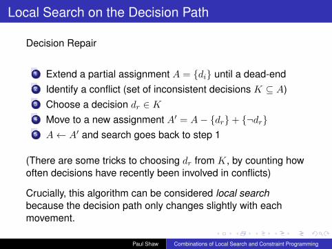
Decision Repair
1 Extend a partial assignment A = {di} until a dead-end2 Identify a conflict (set of inconsistent decisions K ⊆ A)3 Choose a decision dr ∈ K4 Move to a new assignment A′ = A− {dr}+ {¬dr}5 A← A′ and search goes back to step 1
(There are some tricks to choosing dr from K, by counting howoften decisions have recently been involved in conflicts)
Crucially, this algorithm can be considered local searchbecause the decision path only changes slightly with eachmovement.
Paul Shaw Combinations of Local Search and Constraint Programming

Local Search on the Decision Path
Depth-First Search compared to Decision Repair
In tree search, to get to the “goal path”, we must move awayfrom the heuristic search path
- In DFS, this is done bottom-up- In DR, this can be done everywhere on the path
Depth-First Decision Repair
time
initia
l
goal
time
initia
l
goal
Paul Shaw Combinations of Local Search and Constraint Programming

Local Search on the Decision Path
Incomplete Dynamic Backtracking
1 Extend a partial assignment A = {di} until a dead-end2 Choose a subset of decisions D ⊆ A, |D| = b
3 Move to a new smaller assignment A′ = A−D4 A← A′ and search goes back to step 1
Very much like decision repair, but does it act like local search?(The extension in step 1 is done by a value heuristic, soshouldn’t IDS stick closely to the heuristic?)
“We have found that a different type of value ordering heuristic denoted byVH often enhances performance. Instead of finding the best value, itassigns each variable to its last assigned value where possible, withrandom initial values. This speeds the rediscovery of consistentassignments to subsets of variables. However, IDB attempts to use adifferent (randomly-chosen) value for one variable each time a dead-endoccurs; this appears to help by introducing a little variety.” — S. Prestwich
Paul Shaw Combinations of Local Search and Constraint Programming

Local Search on the Decision Path
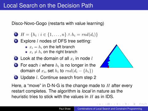
Disco-Novo-Gogo (restarts with value learning)
1 H = {hi : i ∈ {1, . . . , n} ∧ hi = rnd(di)}2 Explore l nodes of DFS tree setting:
xi = hi on the left branchxi 6= hi on the right branch
3 Look at the domain of all xi in node l4 For each i where hi is no longer in the
domain of xi, set hi to rnd(di − {hi})5 Update l. Continue search from step 2
Paul Shaw Combinations of Local Search and Constraint Programming
Local Search on the Decision Path
Disco-Novo-Gogo (restarts with value learning)
1 H = {hi : i ∈ {1, . . . , n} ∧ hi = rnd(di)}2 Explore l nodes of DFS tree setting:
xi = hi on the left branchxi 6= hi on the right branch
3 Look at the domain of all xi in node l4 For each i where hi is no longer in the
domain of xi, set hi to rnd(di − {hi})5 Update l. Continue search from step 2
Here, a “move” in D-N-G is the change made to H after everyrestart completes. The algorithm is local in nature as theheuristic tries to stick with the values in H as in IDS.
Paul Shaw Combinations of Local Search and Constraint Programming
Local Search on the Decision Path
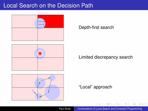
These methods share the ability to allow the current “preferredpath” to creep towards some ideal where conflicts, backtracks,or right branches are avoided as much as possible.
Contrary to chronological backtracking-type methods differentparts of the “preferred path” can be moved towards the idealroughly fairly throughout the search.
Limited Discrepancy Search, although fair in which branchescan be taken to the right, doesn’t have the same ability to“creep” towards an ideal path as it has no notion of a currentpreference.
Paul Shaw Combinations of Local Search and Constraint Programming

Local Search on the Decision Path
Paul Shaw Combinations of Local Search and Constraint Programming
Local Search on the Decision Path
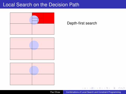
Depth-first search
Paul Shaw Combinations of Local Search and Constraint Programming

Local Search on the Decision Path
Depth-first search
Limited discrepancy search
Paul Shaw Combinations of Local Search and Constraint Programming
Local Search on the Decision Path
Depth-first search
Limited discrepancy search
“Local” approach
Paul Shaw Combinations of Local Search and Constraint Programming

Exploring Neighborhoodsusing CP
Paul Shaw Combinations of Local Search and Constraint Programming
Exploring Neighborhoods using CP
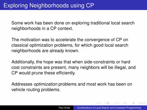
Some work has been done on exploring traditional local searchneighborhoods in a CP context.
The motivation was to accelerate the convergence of CP onclassical optimization problems, for which good local searchneighborhoods are already known.
Additionally, the hope was that when side-constraints or hardcost constraints are present, many neighbors will be illegal, andCP would prune these efficiently.
Addresses optimization problems and most work has been onvehicle routing problems.
Paul Shaw Combinations of Local Search and Constraint Programming

Exploring Neighborhoods using CP
Simple Example - a “change one variable” neighborhood
Given a constraint programming (minimization) problem P with- variables x = 〈x0, . . . , xn〉- Assume w.l.o.g. that x0 is the objective variable- Current solution s = 〈s0, . . . , sn〉
Find best change Minimize x0 subject to
P ∧
(n∑i=1
[xi 6= si] = 1
)
Find any improving change
P ∧ (x0 < s0) ∧
(n∑i=1
[xi 6= si] = 1
)
Paul Shaw Combinations of Local Search and Constraint Programming
Exploring Neighborhoods using CP
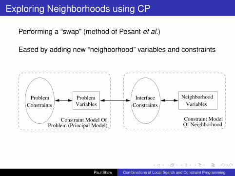
Performing a “swap” (method of Pesant et al.)
Eased by adding new “neighborhood” variables and constraints
Problem Interface Neighborhood
VariablesConstraints Constraints
Problem
Variables
Of NeighborhoodConstraint ModelConstraint Model Of
Problem (Principal Model)
Paul Shaw Combinations of Local Search and Constraint Programming

Exploring Neighborhoods using CP
Performing a “swap” (method of Pesant et al.)
Eased by adding new “neighborhood” variables and constraints
a and b are two new variables with domains {1, . . . , n}. Theyrepresent the indices of the two x variables which swap values.
Neighborhood modela, b ∈ {1, . . . , n}
a < b
Activity constraintsx[a] = s[x[b]]x[b] = s[x[a]]
Quiescence constraints(a = i) ∨ (b = i) ∨ (xi = si) ∀ i ∈ {1, . . . , n}
Paul Shaw Combinations of Local Search and Constraint Programming

Exploring Neighborhoods using CP
Another example: 3-rotation
A B C D E F
Neighborhood modela, b, c ∈ {1, . . . , n}
s[a] < s[b], s[a] < s[c], s[b] 6= s[c]
Activity constraintsx[a] = s[x[b]]x[b] = s[x[c]]x[c] = s[x[a]]
Quiescence constraints(a = i) ∨ (b = i) ∨ (c = i) ∨ (xi = si) ∀ i ∈ {1, . . . , n}
Paul Shaw Combinations of Local Search and Constraint Programming
Exploring Neighborhoods using CP
Generalized TSP insertions (GENIUS-CP)
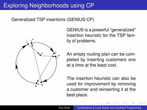
GENIUS is a powerful “generalized”insertion heuristic for the TSP fam-ily of problems.
An empty routing plan can be com-pleted by inserting customers oneat a time at the least cost.
The insertion heuristic can also beused for improvement by removinga customer and reinserting it at thebest place.
Paul Shaw Combinations of Local Search and Constraint Programming

Exploring Neighborhoods using CP
Generalized TSP insertions (GENIUS-CP)
The CP-based neighborhoodmodel allows LS to be carriedout on the CP model, boostingconvergence speed.
Allows great flexibility in the modelcompared to hand coding (e.g.MTW, PDP), so great for trying outnew ideas.
Can be 10x slower than a non-CPhand coded search (GENIUS-TW)
Paul Shaw Combinations of Local Search and Constraint Programming

Exploring Neighborhoods using CP
What causes the inefficiency?
1 CP is quite a heavy deductive technique to use especiallywhen most variables will take a previously known value.
2 The search trees created for most neighborhoods don’thave many branches (and many variables are fixed on thelast branch), so the it is rare to be able to discount a largenumber of illegal neighbors with a single prune.
3 Most “standard” depth-first search explorations of theneighborhood will produce more variable fixings than isstrictly necessary.
Paul Shaw Combinations of Local Search and Constraint Programming

Exploring Neighborhoods using CP
What happens when exploring a neighborhood? Let’s take thesimplest one: changing the value of one of n 0-1 variables.Current solution is A . . .H = 0
A=0
D..H = 0
E..H = 0
F..H = 0
G,H = 0
C..H = 0
B..H = 0
H=1 H = 0
B=1
A=1
C=1
D=1
E=1
F=1F=0
E=0
D=0
C=0
B=0
G=0 G=1
FLIP-8 needs 43 variable fixingsFLIP-n needs n(n+ 3)/2− 1 fixings
Paul Shaw Combinations of Local Search and Constraint Programming
Exploring Neighborhoods using CP
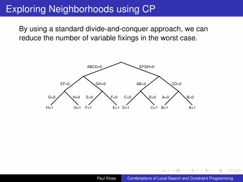
By using a standard divide-and-conquer approach, we canreduce the number of variable fixings in the worst case.
ABCD=0 EFGH=0
EF=0
G=0 H=0
H=1 G=1
GH=0
E=0 F=0
E=1F=1
AB=0 CD=0
A=0 B=0
B=1 A=1
C=0 D=0
D=1 C=1
Paul Shaw Combinations of Local Search and Constraint Programming
Exploring Neighborhoods using CP
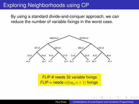
By using a standard divide-and-conquer approach, we canreduce the number of variable fixings in the worst case.
ABCD=0 EFGH=0
EF=0
G=0 H=0
H=1 G=1
GH=0
E=0 F=0
E=1F=1
AB=0 CD=0
A=0 B=0
B=1 A=1
C=0 D=0
D=1 C=1
FLIP-8 needs 32 variable fixingsFLIP-n needs n(log2 n+ 1) fixings
Paul Shaw Combinations of Local Search and Constraint Programming

Exploring Neighborhoods using CP
By using a standard divide-and-conquer approach, we canreduce the number of variable fixings in the worst case.
ABCD=0 EFGH=0
EF=0
G=0 H=0
H=1 G=1
GH=0
E=0 F=0
E=1F=1
AB=0 CD=0
A=0 B=0
B=1 A=1
C=0 D=0
D=1 C=1
In general, when changing a constant number of variables,complexity can be improved from O(nk) to O(nk−1 log n)
Paul Shaw Combinations of Local Search and Constraint Programming

Exploring Neighborhoods using CP
The main advantage to exploring traditional neighborhoodsusing CP is that it is easy to study the behavior of differentneighborhoods on different models, since both models andneighborhoods are simple to create in a CP framework.
But there are practical issues when using it for local search:
When there are few side constraints, a non-CP approach isgenerally less expensive as constraints play a minor roleWhen there are many side constraints, most traditionalneighborhoods get easily stuck in local minimaCP is often too heavy to be competitive without specificoptimizations (even with the above exploration tree)
So...
Paul Shaw Combinations of Local Search and Constraint Programming

Large NeighborhoodSearch
Paul Shaw Combinations of Local Search and Constraint Programming

Large Neighborhood Search
What’s the idea?
(a) Solution (b) Choose (c) Relax (d) Reoptimize
Paul Shaw Combinations of Local Search and Constraint Programming

Large Neighborhood Search
What’s the idea?
(a) Solution (b) Choose (c) Relax (d) Reoptimize
Paul Shaw Combinations of Local Search and Constraint Programming

Large Neighborhood Search
The Basic Algorithm
1 Choose a fragment (mutable elements of the currentsolution)
2 Decide on the “acceptance” criterion3 Use a resource-limited search to try find new values of the
mutable elements under the acceptance criterion4 If a new solution was found, it becomes the current solution5 Go to step 1
Paul Shaw Combinations of Local Search and Constraint Programming

Large Neighborhood Search
LNS is a primarily a local search methodAs such it shares with local search:
AdvantagesTends to find good solutions quicklyHas good scaling propertiesCan exploit meta-heuristic methods
DisadvantagesNot guaranteed to find the optimal (local minima)Needs an initial solution to startDoes not (directly) apply to decision problems
Paul Shaw Combinations of Local Search and Constraint Programming

Large Neighborhood Search
Some particular properties of LNSWith respect to standard local search methods
Is less affected by the local minima problemWhen the problem is constrained, can more easily stay inthe feasible regionIf you have a complete solver already, easy to implement
With respect to complete (CP) methodsVery large problems can be tackled (memory)Less dependent on a good branching heuristicReduces the “horizon” problem of propagationNeeds a neighborhood definition
Paul Shaw Combinations of Local Search and Constraint Programming
Large Neighborhood Search
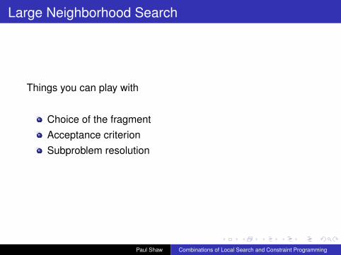
Things you can play with
Choice of the fragmentAcceptance criterionSubproblem resolution
Paul Shaw Combinations of Local Search and Constraint Programming

Large Neighborhood Search
Things you can play with
Choice of the fragmentAcceptance criterionSubproblem resolution
Paul Shaw Combinations of Local Search and Constraint Programming

Large Neighborhood Search
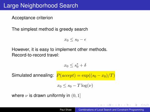
Acceptance criterion
The simplest method is greedy search
x0 ≤ s0 − ε
However, it is easy to implement other methods.Record-to-record travel:
x0 ≤ s∗0 + δ
Simulated annealing:
x0 ≤ s0 − T log(ν)
where ν is drawn uniformly in (0, 1]
Paul Shaw Combinations of Local Search and Constraint Programming
Large Neighborhood Search
Acceptance criterion
The simplest method is greedy search
x0 ≤ s0 − ε
However, it is easy to implement other methods.Record-to-record travel:
x0 ≤ s∗0 + δ
Simulated annealing:
x0 ≤ s0 − T log(ν)
where ν is drawn uniformly in (0, 1]
P (accept) = exp((s0 − x0)/T )
Paul Shaw Combinations of Local Search and Constraint Programming

Large Neighborhood Search
Things you can play with
Choice of the fragmentAcceptance criterionSubproblem resolution
Paul Shaw Combinations of Local Search and Constraint Programming
Large Neighborhood Search
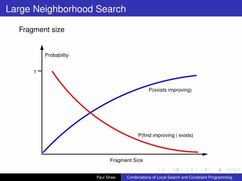
Fragment size
Probability
Fragment Size
1
P(find improving | exists)
P(exists improving)
Paul Shaw Combinations of Local Search and Constraint Programming
Large Neighborhood Search
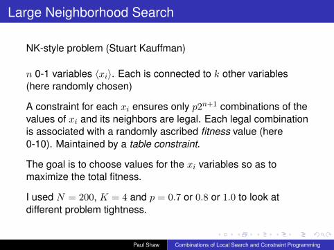
NK-style problem (Stuart Kauffman)
n 0-1 variables 〈xi〉. Each is connected to k other variables(here randomly chosen)
A constraint for each xi ensures only p2n+1 combinations of thevalues of xi and its neighbors are legal. Each legal combinationis associated with a randomly ascribed fitness value (here0-10). Maintained by a table constraint.
The goal is to choose values for the xi variables so as tomaximize the total fitness.
I used N = 200, K = 4 and p = 0.7 or 0.8 or 1.0 to look atdifferent problem tightness.
Paul Shaw Combinations of Local Search and Constraint Programming

Large Neighborhood Search
800
900
1000
1100
1200
1300
1400
1500
0.01 0.1 1 10 100 1000
Fitn
ess
Time (s)
4 variables / 2008 variables / 200
12 variables / 20016 variables / 20020 variables / 20030 variables / 20040 variables / 20060 variables / 20080 variables / 200
Unconstrained (p = 1). Works well from 12-40 variables.
Paul Shaw Combinations of Local Search and Constraint Programming

Large Neighborhood Search
950
1000
1050
1100
1150
1200
1250
1300
1350
0.01 0.1 1 10 100 1000
Fitn
ess
Time (s)
20 variables / 20040 variables / 20060 variables / 20080 variables / 200
100 variables / 200120 variables / 200
Moderately constrained (p = 0.8) Best value looks to be around60 variables
Paul Shaw Combinations of Local Search and Constraint Programming
Large Neighborhood Search
900
950
1000
1050
1100
1150
1200
1250
0.01 0.1 1 10 100 1000
Fitn
ess
Time (s)
20 variables / 20040 variables / 20060 variables / 20080 variables / 200
100 variables / 200120 variables / 200140 variables / 200160 variables / 200
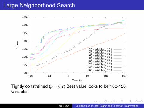
Tightly constrained (p = 0.7) Best value looks to be 100-120variables
Paul Shaw Combinations of Local Search and Constraint Programming

Large Neighborhood Search
Choosing the fragment shape
Simplest method:- Choose the fragment randomly- Can actually work quite well in practice- Easy!
Use problem knowledge (especially when problem structure iswell-known and/or problem is very large compared to thefragment size):
- Try to create “coherent” fragments- Requires a bit more thought- But, beware of bias. Randomize!
Portfolios can be used (see ALNS)
Paul Shaw Combinations of Local Search and Constraint Programming

Large Neighborhood Search
Random selection vs “informed” selection
Random Selection Informed Selection
Paul Shaw Combinations of Local Search and Constraint Programming
Large Neighborhood Search
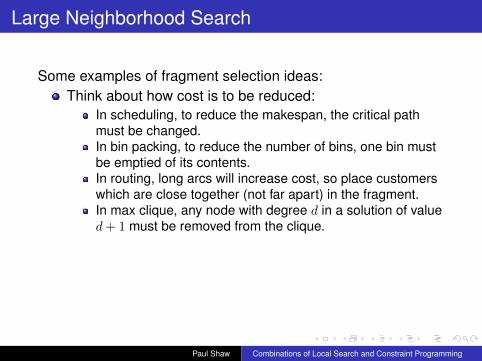
Some examples of fragment selection ideas:Think about how cost is to be reduced:
In scheduling, to reduce the makespan, the critical pathmust be changed.In bin packing, to reduce the number of bins, one bin mustbe emptied of its contents.In routing, long arcs will increase cost, so place customerswhich are close together (not far apart) in the fragment.In max clique, any node with degree d in a solution of valued+ 1 must be removed from the clique.
Paul Shaw Combinations of Local Search and Constraint Programming

Large Neighborhood Search
Some examples of fragment selection ideas:Think about constraints and structure:
Models often have “helper” variables whose values dependon the basic decision variables (e.g. area = wid× height)We must let the values of these variables change!In a constraint
∑i bi = 1, one must include the variable at
value 1 in the fragment.On a timeline, place all elements in a particular timewindow in the fragment.In timetabling or matrix-like problems, relax variablesrelated to one dimension: rooms, resources, days.
Paul Shaw Combinations of Local Search and Constraint Programming
Large Neighborhood Search
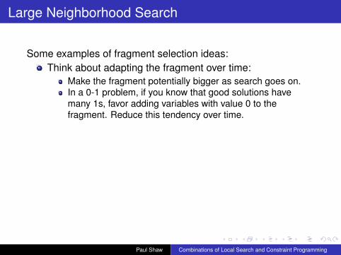
Some examples of fragment selection ideas:Think about adapting the fragment over time:
Make the fragment potentially bigger as search goes on.In a 0-1 problem, if you know that good solutions havemany 1s, favor adding variables with value 0 to thefragment. Reduce this tendency over time.
Paul Shaw Combinations of Local Search and Constraint Programming
Large Neighborhood Search
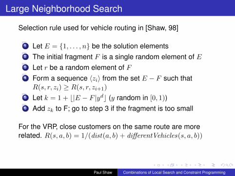
Selection rule used for vehicle routing in [Shaw, 98]
1 Let E = {1, . . . , n} be the solution elements2 The initial fragment F is a single random element of E3 Let r be a random element of F4 Form a sequence 〈zi〉 from the set E − F such thatR(s, r, zi) ≥ R(s, r, zi+1)
5 Let k = 1 + b|E − F |ydc (y random in [0, 1))6 Add zk to F; go to step 3 if the fragment is too small
For the VRP, close customers on the same route are morerelated. R(s, a, b) = 1/(dist(a, b) + differentVehicles(s, a, b))
Paul Shaw Combinations of Local Search and Constraint Programming
Large Neighborhood Search
Things you can play with
Choice of the fragmentAcceptance criterionSubproblem resolution
Paul Shaw Combinations of Local Search and Constraint Programming

Large Neighborhood Search
Subproblem resolution
In a CP context, this is a tree search with propagation.
Typically, depth-first search is used, although other methodslike limited discrepancy search are possible.
The resource limit is normally based on a number of backtracks.- Normally “not too big” values are fine
Variable and value selection rules tend to be a bit lessimportant than in complete search, but if you have good rulesfor the entire problem, you should re-use them here!
- Again, beware of bias. Randomize!
Again, portfolios can be used (see ALNS)
Paul Shaw Combinations of Local Search and Constraint Programming

Large Neighborhood Search
Subproblem resolution
Additional things to consider:Should you take the first improving solution, or find thebest solution in the fragment?To create the fragment, should you build a sub-modelcorresponding to the fragment from scratch? Or have acomplete model, and fix all variables not in the fragment.Impose additional constraints? Say cost = mkspan + late.Then insist cost reduced but mkspan not degraded. Canincrease P (find improving | exist)
In scheduling, although start/end times should be relaxed,we wish to maintain relative order for many tasks: imposethis by adding precedence constraints in the subproblem
Paul Shaw Combinations of Local Search and Constraint Programming

Large Neighborhood Search
What’s the effect of propagation strength on LNS?
I changed the basic NK constraint computing the fitnessfunction at each node from a global table constraintestablishing domain consistency to one expressed indisjunctive form (much weaker)
Paul Shaw Combinations of Local Search and Constraint Programming

Large Neighborhood Search
850
900
950
1000
1050
1100
1150
1200
0.01 0.1 1 10 100 1000
Fitn
ess
Time (s)
20 variables / 20040 variables / 20060 variables / 20080 variables / 200
100 variables / 200120 variables / 200140 variables / 200160 variables / 200
Different fragment sizes with a lower level of consistency.
Paul Shaw Combinations of Local Search and Constraint Programming
Large Neighborhood Search
850
900
950
1000
1050
1100
1150
1200
1250
0.01 0.1 1 10 100 1000
Fitn
ess
Time (s)
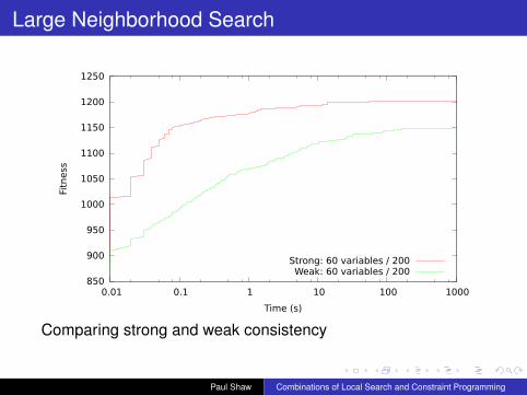
Strong: 60 variables / 200Weak: 60 variables / 200
Comparing strong and weak consistency
Paul Shaw Combinations of Local Search and Constraint Programming

Large Neighborhood Search
850
900
950
1000
1050
1100
1150
1200
1250
0.01 0.1 1 10 100 1000
Fitn
ess
Time (s)
Strong: 100 variables / 200Weak: 100 variables / 200
Comparing strong and weak consistency
Paul Shaw Combinations of Local Search and Constraint Programming
Large Neighborhood Search
850
900
950
1000
1050
1100
1150
1200
1250
0.01 0.1 1 10 100 1000
Fitn
ess
Time (s)
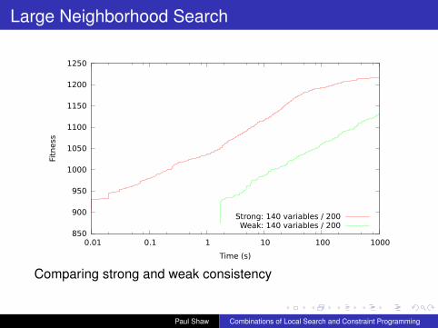
Strong: 140 variables / 200Weak: 140 variables / 200
Comparing strong and weak consistency
Paul Shaw Combinations of Local Search and Constraint Programming

Large Neighborhood Search
Meta-strategies: are they useful for LNS? In particular, canrestarting help?
Paul Shaw Combinations of Local Search and Constraint Programming

Large Neighborhood Search
Meta-strategies: are they useful for LNS? In particular, canrestarting help?
(Maxima are the best of 10 runs)p fragment Fmed Fmax Fmax
size @ 1000s @ 100s @ 10s1.0 30 1422 1431 14290.8 60 1315.5 1337 13140.7 100 1231 1229 1219
Yes! Clearly even a simple restart strategy would help LNS onthe less constrained instances.
Paul Shaw Combinations of Local Search and Constraint Programming

Large Neighborhood Search
Important things about using LNS
The most important thing is the fragment selection. Try tofind the sweet spot. Use domain knowledge it you have it.Use random selection as a baseline. Consider portfolios.The subproblem resolution tends to be less important, butuse a good branching heuristic if you have it. Keep theresource limit reasonable e.g. 100 backtracks.You may be able to apply avoid creating “trivial” fragments.Look out for search stagnation and apply meta-strategies.Easiest is multi-restart.Have some level of randomness everywhere. The benefitof randomness tends increase as search goes on.
Paul Shaw Combinations of Local Search and Constraint Programming

Large Neighborhood Search
Introductory material:
Using constraint programming and local search methods tosolve vehicle routing problems. Paul Shaw. Proceedings ofCP-98, 1998.An adaptive large neighborhood search heuristic for thepickup and delivery problem with time windows. StefanRopke and David Pisinger. Transportation Science, 2006.Large Neighborhood Search. David Pisinger and StefanRopke. Handbook of Metaheuristics, 2010.
Paul Shaw Combinations of Local Search and Constraint Programming
Large Neighborhood Search
Future directions?
LNS for decision problemsConstraining the sub-problemMeta-heuristics adapted to LNSProblem reformulation for LNS suitabilityMachine learning
Paul Shaw Combinations of Local Search and Constraint Programming

Local Search for Pruningand Propagation
Paul Shaw Combinations of Local Search and Constraint Programming

Using Local Search for Pruning and Propagation
Basic idea here is to find a witness which serves as anexistence proof of a result which can be used in pruning orpropagation.
I’ll look at three examples:Prove that certain values cannot be domain-filtered(Galinier et al.)Prove that the current branch cannot lead to a solution(Harvey and Sellmann)Prove that the current branch is dominated by another andcan be pruned (Focacci and Shaw)
Paul Shaw Combinations of Local Search and Constraint Programming

Support Discovery in Some-Different
All-different and some-differentAn “all-different” constraint enforces difference between allpairs of variablesA “some-different” constraint enforces difference betweena specifiable subset of pairs of variablesDomain consistency of “some-different” is NP-complete(equivalent to graph coloring)
Paul Shaw Combinations of Local Search and Constraint Programming

Support Discovery in Some-Different
Let N = {1, 2, . . . , n}, C ⊆ {〈i, j〉 : i, j ∈ N ∧ i < j}, andD = {di : i ∈ N ∧ di ⊂ K} K is a color set.
Some-different can be considered as the domain consistency ofthe coloring problem P :
Find x = 〈x1, . . . , xn〉 such that
∀i∈N xi ∈ di
∀〈i,j〉∈C xi 6= xj
The domain consistency problem DC(P ) is then to either provethat P has no solution or to find reduced domainsd′ = 〈d′1, . . . , d′n〉 such that d′i ⊆ di and k ∈ d′i if and only if thereis a solution x to P with xi = k.
Paul Shaw Combinations of Local Search and Constraint Programming
Support Discovery in Some-Different
Each complete coloring x gives a point coloring 〈i, xi〉 for eachnode i.
By finding as many complete colorings as possible, we hope tocheaply identify many unique point colorings and thus requiredvalues ri for each node i.
The reduced domain will be contained between these requiredvalues and the initial domain: ri ⊆ d′i ⊆ di.
Complete colorings are found using tabu search which stopswhen either we know that ∀i∈N d′i = di or when a number ofiterations pass without finding any new required member.
Paul Shaw Combinations of Local Search and Constraint Programming

Support Discovery in Some-Different
The tabu search process tries to minimize two differentobjectives which are blended together.
Let L ⊆ {〈i, k〉 : i ∈ N ∧ k ∈ d′j} be the set of point coloringsfound up to the current point in the algorithm. The cost functionused is:
f(x) =
α ∑〈i,j〉∈C
[xi = xj ]
+ |L ∩ {〈i, xi〉 : i ∈ N}|
α is adjusted according to the difficulty of finding completeassignments.
Paul Shaw Combinations of Local Search and Constraint Programming

Support Discovery in Some-Different
After tabu search, if ∃i∈N ri 6= di, then for each k ∈ (di − ri), xiis fixed to k and a complete search determines if the remainingproblem can be colored
If the subproblem cannot be colored, k 6∈ d′i
If the subproblem can be colored, k ∈ d′i and the coloring isused to enrich 〈ri〉.
Paul Shaw Combinations of Local Search and Constraint Programming

Social Golfers: Pruning and propagation
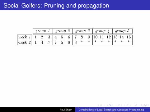
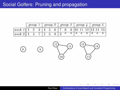
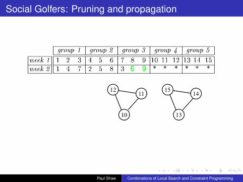
How can nm golfers play in m groups of n golfers each weekover p weeks such that no golfer plays with another more thanonce?
Solution to a 5-3-7 problem.
group 1 group 2 group 3 group 4 group 5week 1 1 2 3 4 5 6 7 8 9 10 11 12 13 14 15week 2 1 4 8 2 5 11 3 9 15 6 12 14 7 10 13week 3 1 5 13 2 8 14 3 7 11 4 9 12 6 10 15week 4 1 6 9 2 12 15 3 8 10 4 11 13 5 7 14week 5 1 7 12 2 4 10 3 6 13 5 8 15 9 11 14week 6 1 10 14 2 9 13 3 5 12 4 7 15 6 8 11week 7 1 11 15 2 6 7 3 4 14 5 9 10 8 12 13
Paul Shaw Combinations of Local Search and Constraint Programming
Social Golfers: Pruning and propagation
Paul Shaw Combinations of Local Search and Constraint Programming
Social Golfers: Pruning and propagation
Paul Shaw Combinations of Local Search and Constraint Programming

Social Golfers: Pruning and propagation
6
DummyDummyDummy
Paul Shaw Combinations of Local Search and Constraint Programming
Social Golfers: Pruning and propagation
6 9
Dummy DummyDummy
Paul Shaw Combinations of Local Search and Constraint Programming

Social Golfers: Pruning and propagation
6 9
The clique 10-11-12needs three opengroups
10 1112?
Paul Shaw Combinations of Local Search and Constraint Programming
Social Golfers: Pruning and propagation
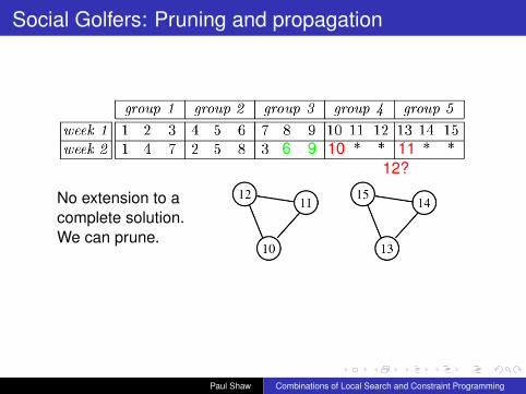
6 9
No extension to acomplete solution.We can prune.
10 1112?
Paul Shaw Combinations of Local Search and Constraint Programming
Social Golfers: Pruning and propagation
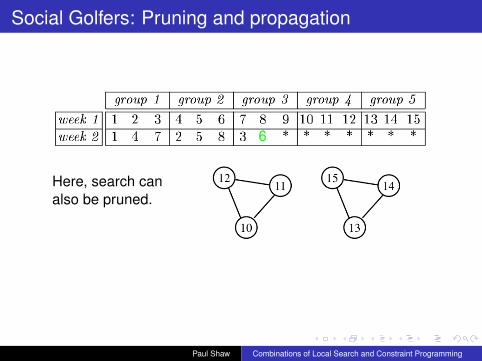
6
Here, search canalso be pruned.
Paul Shaw Combinations of Local Search and Constraint Programming

Social Golfers: Pruning and propagation
6
Here, search canalso be pruned.Group 3 needs tohave two emptyplaces, one for each3-clique
10 11 13 12 1415?
Paul Shaw Combinations of Local Search and Constraint Programming

Social Golfers: Pruning and propagation
Even here we cando something.Propagate!
Paul Shaw Combinations of Local Search and Constraint Programming

Social Golfers: Pruning and propagation
6= 6, 6= 9
Members of the two3-cliques take up thetwo remaining slotsin the third group.Therefore, neithergolfer 6 nor golfer 9can be assigned tothe third group.
Paul Shaw Combinations of Local Search and Constraint Programming

Social Golfers: Pruning and propagation
6= 6, 6= 9
Cliques arediscovered by localsearch through anoscillation-basedprocess ofexpanding andcontracting apotential clique.
Paul Shaw Combinations of Local Search and Constraint Programming
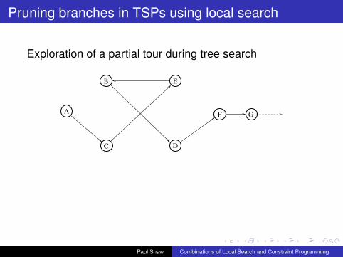
Pruning branches in TSPs using local search
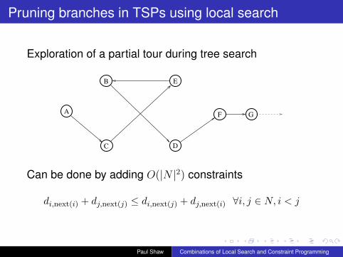
Exploration of a partial tour during tree search
B
C
A
E
D
F G
Paul Shaw Combinations of Local Search and Constraint Programming

Pruning branches in TSPs using local search
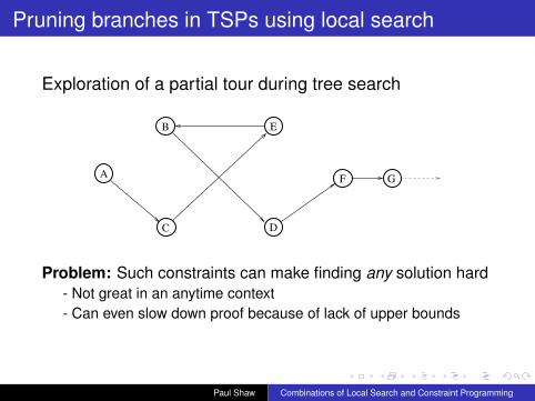
Exploration of a partial tour during tree search
B
C
A
E
D
F G
We would like to avoid partial tours like this!
Reasoning: Tours with crossed arcs are not locally optimalAnd locally optimal solutions cannot be globally optimal
Paul Shaw Combinations of Local Search and Constraint Programming
Pruning branches in TSPs using local search
Exploration of a partial tour during tree search
B
C
A
E
D
F G
Can be done by adding O(|N |2) constraints
di,next(i) + dj,next(j) ≤ di,next(j) + dj,next(i) ∀i, j ∈ N, i < j
Paul Shaw Combinations of Local Search and Constraint Programming
Pruning branches in TSPs using local search
Exploration of a partial tour during tree search
B
C
A
E
D
F G
Problem: Such constraints can make finding any solution hard- Not great in an anytime context- Can even slow down proof because of lack of upper bounds
Paul Shaw Combinations of Local Search and Constraint Programming

Pruning branches in TSPs using local search
Exploration of a partial tour during tree search
B
C
A
E
D
F G
Basic idea: Disallow the current partial tour if it is not locallyoptimal and the improved tour has already been exploredearlier in the search tree
Paul Shaw Combinations of Local Search and Constraint Programming

Pruning branches in TSPs using local search
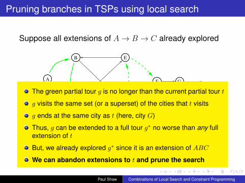
Suppose all extensions of A→ B → C already explored
B
C
A
E
D
F G
Paul Shaw Combinations of Local Search and Constraint Programming

Pruning branches in TSPs using local search
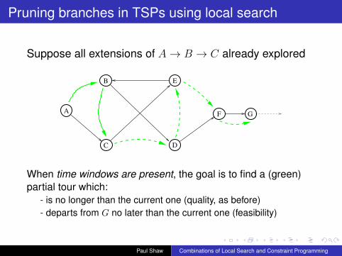
Suppose all extensions of A→ B → C already explored
B
C
A
E
D
F G
Add cities in the current tour not in ABC to the green tour- In any order, ensuring that G (last city) remains last- Now, the green tour has at least all the cities of the current partial
tour
Paul Shaw Combinations of Local Search and Constraint Programming

Pruning branches in TSPs using local search
Suppose all extensions of A→ B → C already explored
B
C
A
E
D
F G
Perform local search on the green partial tour, but don’t moveABC or G
Paul Shaw Combinations of Local Search and Constraint Programming

Pruning branches in TSPs using local search
Suppose all extensions of A→ B → C already explored
B
C
A
E
D
F G
Perform local search on the green partial tour, but don’t moveABC or G
The goal is to find a partial tour shorter than the current one
Paul Shaw Combinations of Local Search and Constraint Programming
Pruning branches in TSPs using local search
Suppose all extensions of A→ B → C already explored
B
C
A
E
D
F G
The green partial tour g is no longer than the current partial tour t
g visits the same set (or a superset) of the cities that t visits
g ends at the same city as t (here, city G)
Thus, g can be extended to a full tour g∗ no worse than any fullextension of t
But, we already explored g∗ since it is an extension of ABC
We can abandon extensions to t and prune the search
Paul Shaw Combinations of Local Search and Constraint Programming
Pruning branches in TSPs using local search
Suppose all extensions of A→ B → C already explored
B
C
A
E
D
F G
When time windows are present, the goal is to find a (green)partial tour which:
- is no longer than the current one (quality, as before)- departs from G no later than the current one (feasibility)
Paul Shaw Combinations of Local Search and Constraint Programming

Local Search andDominance
Paul Shaw Combinations of Local Search and Constraint Programming

Local Search and Dominance
Let’s look at this again
B
C
A
E
D
F G
We can add constraints to avoid crossed arcs (although it mightbe a bad idea in that particular case).
Is there a generalization?
This idea has been used for a long time. A formalism waspublished by Chu and Stuckey at CP 2012.
Paul Shaw Combinations of Local Search and Constraint Programming

Local Search and Dominance
The idea itself is really simple: we don’t want to exploreassignments which can be bettered via a local search move, solet’s add constraints which disallow these assignments
The move considered must preserve feasibility too. We need toensure that if the assignment before the move was feasible,then so will the assignment after the move.
Essentially:
If then new assignment is strictly better and at least asfeasible as the original assignment, the original assign-ment should be forbidden.
Paul Shaw Combinations of Local Search and Constraint Programming

Local Search and Dominance
Method:
Assume a problem P , a function f to minimize and anassignment sΘ is a set of transformations likely to map solutions tobetter solutionsFor each θ ∈ Θ
Find constraint κF obeying (P (s) ∧ κF (s))⇒ P (θ(s))
Find constraint κI obeying (P (s) ∧ κI(s))⇒ f(θ(s)) < f(s)
Add the constraint ¬κF ∧ ¬κI
Paul Shaw Combinations of Local Search and Constraint Programming

Local Search and Dominance
ExamplesKnapsackBin packingMaximum independent setMax-cut
Paul Shaw Combinations of Local Search and Constraint Programming
Local Search and Dominance
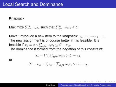
Knapsack
Maximize∑n
i=1 vixi such that∑n
i=1wixi ≤ C
Move: introduce a new item to the knapsack: xk = 0→ xk = 1The new assignment is of course better if it is feasible. It isfeasible if xk = 0 ∧
∑i 6=k wixi ≤ C − wk.
The dominance if formed from the negation of this constraint:
xk = 1 ∨∑
i 6=k wixi > C − wkor
(C − wk + 1)xk +∑
i 6=k wixi > C − wk
Paul Shaw Combinations of Local Search and Constraint Programming

Local Search and Dominance
Knapsack II
Maximize∑n
i=1 vixi such that∑n
i=1wixi ≤ C
Move: Swap the positions (in/out) of two objects j and k
Better if value goes up:vjxk + vkxj > vjxj + vkxk
Definitely feasible if weight does not go up:wjxk + wkxj ≤ wjxj + wkxk
Taking the combination and negating (new configuration mustbe no better or less feasible than previous), we get:
wi ≥ wj ∧ vi < vj ⇒ xi ≤ xj
Paul Shaw Combinations of Local Search and Constraint Programming
Local Search and Dominance
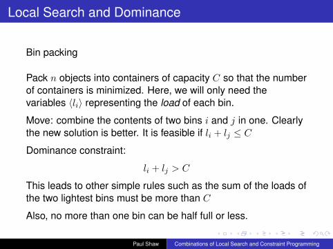
Bin packing
Pack n objects into containers of capacity C so that the numberof containers is minimized. Here, we will only need thevariables 〈li〉 representing the load of each bin.
Move: combine the contents of two bins i and j in one. Clearlythe new solution is better. It is feasible if li + lj ≤ C
Dominance constraint:
li + lj > C
This leads to other simple rules such as the sum of the loads ofthe two lightest bins must be more than C
Also, no more than one bin can be half full or less.
Paul Shaw Combinations of Local Search and Constraint Programming

Local Search and Dominance
Maximum independent set
Maximize∑n
i=1 xi with xi ∈ {0, 1} and ∀〈j, k〉 ∈ E, xi + xj ≤ 1
Paul Shaw Combinations of Local Search and Constraint Programming

Local Search and Dominance
Maximum independent set
Maximize∑n
i=1 xi with xi ∈ {0, 1} and ∀〈j, k〉 ∈ E, xi + xj ≤ 1
Move: add a new node k to the independent set. The movenecessarily leads to a better solution. It is feasible if it does notconflict with another node in the independent set.
(xk = 0) ∧∑{j:〈j,k〉∈E} xj = 0
Negating, the dominance constraint becomes:
xk +∑{j:〈j,k〉∈E} xj ≥ 1
Paul Shaw Combinations of Local Search and Constraint Programming
Local Search and Dominance
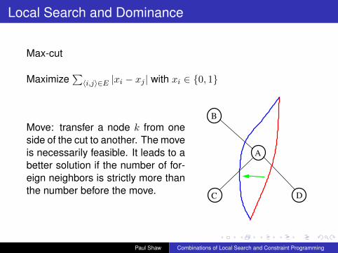
Max-cut
Maximize∑〈i,j〉∈E |xi − xj | with xi ∈ {0, 1}
Move: transfer a node k from oneside of the cut to another. The moveis necessarily feasible. It leads to abetter solution if the number of for-eign neighbors is strictly more thanthe number before the move.
B
C
A
D
Paul Shaw Combinations of Local Search and Constraint Programming

Local Search and Dominance
Max-cut
Maximize∑〈i,j〉∈E |xi − xj | with xi ∈ {0, 1}
Let νi be an integer set containing the neighbors of node i andthe number of “right” neighbors is σi =
∑j∈νi xj
The move is better if:((xi = 0) ∧ σj < |νi|
2 ) ∨ ((xi = 1) ∧ σj > |νi|2 )
Negating, the dominance constraint is:((xi = 0)⇒ σi ≥ |νi|2 ) ∧ ((xi = 1)⇒ σi ≤ |νi|2 )
Which reduces to:|νi|2 ≤
|νi|2 xi + σi ≤ |νi|
B
C
A
D
Paul Shaw Combinations of Local Search and Constraint Programming
Local Search and Dominance
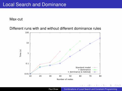
Max-cut
Different runs with and without different dominance rules
0.01
0.1
1
10
100
10 20 30 40 50 60 70 80
Tim
e (
s)
Number of nodes
Standard model+ dominance
+ dominance & tiebreak
Paul Shaw Combinations of Local Search and Constraint Programming

Combinations of Local Search and ConstraintProgramming
Masterclass on Hybrid Methods, Toulouse, 4-5 June 2018
Paul Shaw
IBM Analytics, France
Paul Shaw Combinations of Local Search and Constraint Programming