1Si“ambpp Hsdemaa WctfcrS Tbir

A. Yanagawa, S.-F. Chang, L. Kennedy, and W. Hsu ”Columbia University’s Baseline detectors for 374 LSCOMSemantic Visual Concepts,” Columbia University ADVENT Technical Report # 222-2006-8, March 20, 2007.

Columbia University’s Baseline Detectors for 374 LSCOM Semantic Visual Concepts

Akira Yanagawa, Shih-Fu Chang, Lyndon Kennedy and Winston Hsu

{akira, sfchang, lyndon and winston@ee.columbia.edu} Columbia University ADVENT Technical Report # 222-2006-8

March 20, 2007

(Download site- http://www.ee.columbia.edu/dvmm/columbia374)

. Introduction emantic concept detection represents a key requirement in accessing large collections of digital

mages/videos. Automatic detection of presence of a large number of semantic concepts, such as person,” or “waterfront,” or “explosion”, allows intuitive indexing and retrieval of visual content t the semantic level. Development of effective concept detectors and systematic evaluation ethods has become an active research topic in recent years. For example, a major video retrieval

enchmarking event, NIST TRECVID[1], has contributed to this emerging area through (1) the rovision of large sets of common data and (2) the organization of common benchmark tasks to erform over this data.

owever, due to limitations on resources, the evaluation of concept detection is usually much maller in scope than is generally thought to be necessary for effectively leveraging concept etection for video search. In particular, the TRECVID benchmark has typically focused on valuating, at most, 20 visual concepts, while providing annotation data for 39 concepts. Still, any researchers believe that a set of hundreds or thousands of concept detectors would be more

ppropriate for general video retrieval tasks. To bridge this gap, several efforts have developed nd released annotation data for hundreds of concepts [2, 5, 6].

hile such annotation data is certainly valuable, it should also be noted that building automatic oncept detectors is a complicated and computationally expensive process. Research results over he last few years have converged on the finding that an approach using grid- and global-level eature representations of keyframes from a video shot and a support vector machine (SVM) lassifier provide an adequate baseline for building a strong concept detection system [8, 3]. The esulting situation is many research groups investing serious effort in replicating these baseline VM-based methods, which leaves little time for investigating new and innovative approaches.

he Mediamill Challenge dataset [2] helped address much of this replication-of-effort problem y releasing detectors for 101 semantic concepts over the TRECVID2005/2006 dataset[1], ncluding the ground truth, the features, and the results of the detectors. This dataset is useful for educing the large computational costs in concept detection and allowing for a focus on

1

innovative new approaches. In this same spirit, we are releasing a set of 374 semantic concept detectors (called “Columbia374”) with the ground truth, the features, and the results of the detectors based on our baseline detection method in TRECVID2005/2006 [3, 4], with the goal of fostering innovation in concept detection and enabling the exploration of the use of a large set of concept detectors for video search. When future datasets become available (e.g., TRECVID 2007), we will also release features and detection results over the new data set. The 374 concepts are selected from the LSCOM ontology [6], which includes more than 834 visual concepts jointly defined by researchers, information analysts, and ontology specialists according to the criteria of usefulness, feasibility, and observability. These concepts are related to events, objects, locations, people, and programs that can be found in general broadcast news videos. The definition of the LSCOM concept list and the annotation of its subset (449 concepts) may be found on [5]. Columbia374 employs a simple baseline method, composed of three types of features, individual SVMs [7] trained independently over each feature space, and a simple late fusion of the SVMs. Such an approach is rather light-weight, when compared to top-performing TRECVID submissions. Nonetheless, running even such a light-weight training process for all 374 concepts takes approximately 3 weeks using 20 machines in parallel, or roughly more than a year of machine time. Clearly this is not an effort that needs to be duplicated at dozens of research groups around the world. Despite the simple features and classification methods used for the Columbia374 detectors, the resulting baseline models achieve very good performance in the TRECVID2006 concept detection benchmark and, therefore, provides a strong baseline platform for researchers to expand upon. The remainder of the paper is structured as follows. In Section 2, we discuss the details of the design and implementation of the concept detection models. In Section 3, we give detailed information about the contents of the Columbia374 distribution, which includes all features and annotations used, as well as the resulting SVM models and the scores on the test data. Finally, in Section 4, we provide some evaluation of the Columbia374 models directly for concept detection as well as for providing context in concept detection and automatic search. 2. Model Development 2.1. Experimental Data The Columbia374 concept detectors are developed and tested using the TRECVID2005 and 2006 data sets, which contain a combined total of nearly 330 hours of broadcast news video gathered from more than a dozen news programs in three different languages. The TRECVID2005 set is composed of 277 video clips. They were separated into two main groups by NIST: (1) the development set, for which many ground-truth annotations are available for system development, and (2) the test set, which system developers are not supposed to view prior to testing their system (in order to avoid bias in development. The TRECVID2006 dataset comes as one large test set, relying on the TRECVID2005 data for system development. Since only the TRECVID2005 development set contains annotations, it needs to be further sub-divided into sections for developing and validating learning-based models for concept detection. We adopt

2

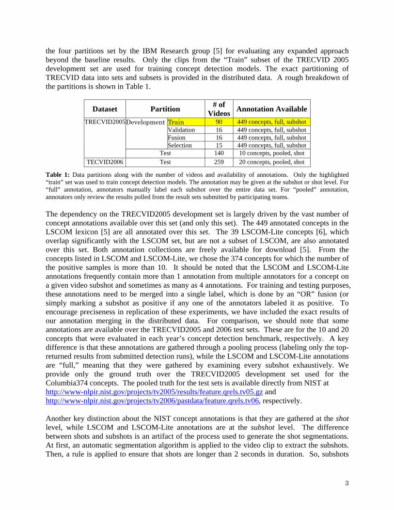
the four partitions set by the IBM Research group [5] for evaluating any expanded approach beyond the baseline results. Only the clips from the “Train” subset of the TRECVID 2005 development set are used for training concept detection models. The exact partitioning of TRECVID data into sets and subsets is provided in the distributed data. A rough breakdown of the partitions is shown in Table 1.

Dataset Partition # of Videos Annotation Available

Train 90 449 concepts, full, subshot Validation 16 449 concepts, full, subshot Fusion 16 449 concepts, full, subshot

Development

Selection 15 449 concepts, full, subshot

TRECVID2005

Test 140 10 concepts, pooled, shot TECVID2006 Test 259 20 concepts, pooled, shot

Table 1: Data partitions along with the number of videos and availability of annotations. Only the highlighted “train” set was used to train concept detection models. The annotation may be given at the subshot or shot level. For “full” annotation, annotators manually label each subshot over the entire data set. For “pooled” annotation, annotators only review the results polled from the result sets submitted by participating teams. The dependency on the TRECVID2005 development set is largely driven by the vast number of concept annotations available over this set (and only this set). The 449 annotated concepts in the LSCOM lexicon [5] are all annotated over this set. The 39 LSCOM-Lite concepts [6], which overlap significantly with the LSCOM set, but are not a subset of LSCOM, are also annotated over this set. Both annotation collections are freely available for download [5]. From the concepts listed in LSCOM and LSCOM-Lite, we chose the 374 concepts for which the number of the positive samples is more than 10. It should be noted that the LSCOM and LSCOM-Lite annotations frequently contain more than 1 annotation from multiple annotators for a concept on a given video subshot and sometimes as many as 4 annotations. For training and testing purposes, these annotations need to be merged into a single label, which is done by an “OR” fusion (or simply marking a subshot as positive if any one of the annotators labeled it as positive. To encourage preciseness in replication of these experiments, we have included the exact results of our annotation merging in the distributed data. For comparison, we should note that some annotations are available over the TRECVID2005 and 2006 test sets. These are for the 10 and 20 concepts that were evaluated in each year’s concept detection benchmark, respectively. A key difference is that these annotations are gathered through a pooling process (labeling only the top-returned results from submitted detection runs), while the LSCOM and LSCOM-Lite annotations are “full,” meaning that they were gathered by examining every subshot exhaustively. We provide only the ground truth over the TRECVID2005 development set used for the Columbia374 concepts. The pooled truth for the test sets is available directly from NIST at http://www-nlpir.nist.gov/projects/tv2005/results/feature.qrels.tv05.gz and http://www-nlpir.nist.gov/projects/tv2006/pastdata/feature.qrels.tv06, respectively. Another key distinction about the NIST concept annotations is that they are gathered at the shot level, while LSCOM and LSCOM-Lite annotations are at the subshot level. The difference between shots and subshots is an artifact of the process used to generate the shot segmentations. At first, an automatic segmentation algorithm is applied to the video clip to extract the subshots. Then, a rule is applied to ensure that shots are longer than 2 seconds in duration. So, subshots

3

which are longer than 2 seconds become shots, while subshots shorter than two seconds are merged with adjacent subshots to compose a shot. A shot may contain only one or many subshots. A keyframe (or a still image to represent the segment) is extracted for each subshot and shot using the I-frame closest to the center of the segment. The shot segmentation and formatting are contributed by Christian Petersohn at the Fraunhofer (Heinrich Hertz) Institute in Berlin [9] and the Dublin City University team. For more details about the segmentation, refer to the guidelines for the TRECVID 2006 Evaluation at http://www-nlpir.nist.gov/projects/tv2006/tv2006.html. Figure 1 shows an overview of the composition of shots and subshots.

Subshot1 Subshot2 Subshot3 Subshot4

1sec 2.5sec 1sec 1.5sec

Shot1 Shot4

3.5sec 2.5sec

Subshot1 Subshot2 Subshot3 Subshot4

1sec 2.5sec 1sec 1.5sec

Subshot1 Subshot2 Subshot3 Subshot4

1sec 2.5sec 1sec 1.5sec

Shot1 Shot4

3.5sec 2.5sec

Shot1 Shot4

3.5sec 2.5sec Fig. 1: Visualization of the composition of shots and subshots in TRECVID data.

In the Columbia374 models, the ground truth, the visual features, the trained SVM models and the result of the detectors are provided based on the keyframes of subshots; however, the official TRECVID evaluations are based on shot level labels. Therefore, when we evaluate the accuracy of Columbia374 using TRECVID procedures, we aggregated the results of various subshots in a single shot by using max fusion: simply taking the maximum score of all subshots within a shot to be the score for the shot. 2.2. Visual Features The Columbia374 models are trained using three visual features: edged direction histogram (EDH), Gabor (GBR), and grid color moment (GCM). For information about these features in detail, please refer to [10]. 2.3. Concept Models The Columbia374 models are implemented by training SVM classifiers individually over each of the three feature spaces described in Section 2.2 and averaging the resulting scores from each model. The SVMs are implemented using LIBSVM (Version 2.81) [7] and the resulting support vectors and parameters are provided in the data distribution. This process of training models for 374 concepts took twenty days, using all keyframes in “train” partition and 20 single CPU computers (2.6Ghz Pentium4). In the following section, the training procedure is discussed in detail.

4

2.3.1. Training Procedure Our training procedure accounts for a number of factors, including the distribution of training examples, the normalization of the input feature space, and the selection of model parameters. 2.3.1.1. Choosing Training Examples When training SVM models, it is important to maintain balance between the number of positive and negative examples provided. In general, however, the annotations in the LSCOM and LSCOM-Lite lexicons are highly skewed towards negative examples (on average: 2% positive examples and 98% negative). In our implementation, we utilized all available positive examples and randomly sampled the negative examples. There are three procedures for selecting negative samples, which rely on the natural distribution of positive and negative examples for a given concept. The procedures are as follows: Take 20 % of negative samples randomly. Then

i. If the number of examples in the 20% negative set is more than the number of positive examples, the 20% negative samples were used for training.

ii. If the number of examples in the 20% negative set is less than the number of positive examples, and the total number of negative examples is greater than the number of positive samples, we randomly chose a set of negative examples equal in size to the number of positive examples.

iii. If the number of negative examples is less than the number of positive examples, we chose all available negative samples.

2.3.1.2. Feature Normalization SVMs work best with features that are roughly in the same dynamic range, which is not typically the case with the raw features that we have chosen. To address this, we have normalized the features using statistical normalization: using the sample mean (µ ) and standard deviation (σ ) to adjust each feature dimension to have zero-valued mean and unit standard deviation. Consider a feature vector (with m dimensions): ( )imiiii xxxxx ,,,, 321 L= . The sample mean vector (µ ) and the standard deviation vector (σ ) are:

∑=

=N

iix

N 1

1µ , ( )∑=

−=N

iix

N 1

21 µσ

To acquire normalized feature vectors ( ), we plugged feature vectors into: Nx

( )σµ−

=xxN

The division operation above is applied to each element of the vector respectively.

5

2.3.1.3. Parameter Selection The reliability of learned SVM models can be highly subject to the selection of model parameters. In our models, we used RBF kernels, which have to primary parameters: C (the cost parameter in soft-margin SVMs) and γ (the width of the RBF function). To set these parameters, we conducted a grid search with k-fold cross validation, wherein we trained a model on part of the “train” and tested the learned model on the left-out set. This process was repeated 5 times, with a different portion of the train set left out for testing on each iteration. From this process, we determined which parameter settings gave the best performance. Finally we retrained a model using the entire Train partition with the best parameter set and applied the learned model to all other sets. Figure 2 shows the general flow of this cross-validation parameter search process. Therefore, users of these resulting models and scores should note that for each concept, scores on all sets (except for “train”) are generated using the same model, and, therefore, scores on different subshots within these sets should be comparable. Please note that scores are also provided over the “train” partition. But note these scores are obtained from the model learned from the “train” partition itself mentioned earlier. Therefore, such scores should be used differently from the test scores from other sets. The resulting models and scores are all included in the distributed data.

Train Validation Fusion SelectionTrain

1Train

2Train

3Train

4Train

5

Train1

Train2

Train3

Train4

Train5

TrainingValidation

Randomly divide into 5 subsets

With varying C and γ

DevelopmentTRECVID2005

Select the Best (C,γ)

Based on Average Precision

Train2

Train3

Train4

Train5

Train1

With varying C and γ

Train3

Train4

Train5

Train1

Train2

With varying C and γ

Train4

Train5

Train1

Train2

Train3

With varying C and γ

Train5

Train1

Train2

Train3

Train4

With varying C and γ

Train1

Train2

Train3

Train4

Train5

Train Validation Fusion SelectionTrain

1Train

2Train

3Train

4Train

5

Train1

Train2

Train3

Train4

Train5

Train2

Train3

Train4

Train5

TrainingValidation

Randomly divide into 5 subsets

With varying C and γ

DevelopmentTRECVID2005

Select the Best (C,γ)

Based on Average Precision

Retrain on Train partition with the Best (C,γ)

Train2

Train3

Train4

Train5

Train1

Train3

Train4

Train5

Train1

With varying C and γ

Train3

Train4

Train5

Train1

Train2

Train4

Train5

Train1

Train2

With varying C and γ

Train4

Train5

Train1

Train2

Train3

Train5

Train1

Train2

Train3

With varying C and γ

Train5

Train1

Train2

Train3

Train4

Train1

Train2

Train3

Train4

With varying C and γ

Train1

Train2

Train3

Train4

Train5

Train1

Train2

Train3

Train4

Train5

Retrain on Train partition with the Best (C,γ)

Fig. 2: Parameter selection process, using 5-fold cross-validation over the “train” partition.

2.3.2. Detection Scores and Late Fusion As noted above, we have learned separate models for each feature (grid color moments, edge direction histogram, and texture); however, we would like to combine all of these resulting models to give a fused score. In [11], late fusion (the combination of separate scores) was shown

6

to perform favorably when compared to early fusion (the combination of many features into one large feature vector. Therefore, we adopt a late fusion approach for generating fused scores. To fuse the results, we simply average the scores resulting from each classifier. This is shown in Figure 3. This averaging approach is, of course, subject to the comparability in dynamic ranges between the outputs of various SVM classifiers. To address this, we normalize the scores through the sigmoid function as shown in [12], i.e.

( )BAfSN ++

=exp1

1

Where, and are normalized score and raw scores respectively, and A, B are the parameters to control the shape of the sigmoid function. In our approach we used 1 and 0 for A and B respectively in order to avoid over-fitting.

NS f

Average Fusion

Texture Color Edge

Classifier Classifier Classifier

Scores Scores Scores

Average Fusion

Texture Color Edge

Classifier Classifier Classifier

Scores Scores Scores

Fig. 3: Late fusion of multiple classifiers.

3. Performance Evaluation and Applications As of this writing, the Columbia374 models have been used and evaluated in a number of applications. They have been directly evaluated for detection accuracy in the TRECVID2006 benchmark and indirectly evaluated for their utility in providing context for improving concept detection and search applications. 3.1. TRECVID2006 Evaluation We apply the Columbia374 models to the TRECVID2006 test set for each of the 20 concepts officially evaluated in the benchmark. The models were also used as a baseline to be improved upon by adding in additional new methods. Figure 4 shows the resulting performance of the Columbia374 models (in green), along with the improved runs (in red, which were all reinforced by the Columbia374 models) as well as all official TRECVID submissions (in Pale Blue). The performance scores are shown in inferred Average Precision, which is an adaptation of Average Precision and a method for estimating the area underneath the precision-recall curve. This is the official metric used in the TRECVID2006 evaluation. For more details, see http://www-nlpir.nist.gov/projects/tv2006/infAP.html.

7

0

0.02

0.04

0.06

0.08

0.1

0.12

0.14

0.16

0.18

0.2

Run

Mean A

vera

ge P

recis

ion

A_CL1_1

A_CL2_2

A_CL3_3

A_CL4_4

A_CL5_5

A_CL6_6

Columbia374

Fig. 4: Performance of the Columbia374 models, Columbia official runs, and all official TRECVID2006 concept

detection systems. Table 2 lists each of the methods used to improve upon the Columbia374 baseline. Results from these methods constitute the six official runs (A_CL1_1 to A_CL6_6) we submitted to the TRECVID evaluation task of high-level feature detection. Each of these methods is discussed in greater detail in [4]. Note the last run (A_CL6_6) implements the same baseline approach as that used in developing Columbia 374. Minor differences between the two are the expanded size of negative data sets (40% instead of 20%) used in A_CL6_6 and its fusion with another baseline model using a single SVM over a long feature vector aggregating all three features (color, texture, and edge). These various approaches add up to roughly a 40% relative improvement in detection performance and demonstrate the power of testing new approaches on top of a strong baseline. The “Boosted Conditional Random Field” method [13] is unique among these methods in that it incorporates the detection scores from all 374 baseline models (instead of just the one score for the concept being detected). We will discuss this approach further in the following section.

Run Description

A_CL1_1 Choose the best-performing classifier for each concept from all the following runs and an event detection method (Event Detection utilizing Earth Mover's Distance [15]).

A_CL2_2 Choose the best-performing visual-based classifier for each concept from runs A_CL4_4, A_CL5_5, and A_CL6_6. (Best Visual Only)

A_CL3_3 Weighted average fusion of visual-based classifier A_CL4_4 with a text classifier. (Visual + Text)

A_CL4_4 Average fusion of A_CL5_5 with a lexicon-spatial pyramid matching approach that incorporates local feature and pyramid matching (Lexicon-Spatial Pyramid Match Kernel).

A_CL5_5 Average fusion of A_CL6_6 with a context-based concept fusion approach that incorporates inter-conceptual relationships to help detect individual concepts (Boosted Conditional Random Field).

8

A_CL6_6

Average fusion of two SVM baseline classification results for each concept: (1) a fused classification result by averaging 3 single SVM classification results. Each SVM classifier uses one type of color/texture/edge features and is trained on the whole training set with 40% negative samples; (2) a single SVM classifier using color and texture trained on the whole training set (90 videos) with 20% negative samples(Columbia374 + Another Baseline).

Table 2: Description of each of Columbia’s TRECVID 2006 submitted runs built on top of the Columbia 374 baseline.

3.2. Applications in Extracting Context from Concept Detectors An additional benefit of a large collection of concept detectors, such as the Columbia374 set, is that the resulting detection scores can provide many semantic cues about the contents of images and videos, which can be further used to add context for concept detection or automatic search. In the Boosted Conditional Random Field (BCRF) model [13], the entire collection of 374 detection scores are applied to provide context and help in the detection of individual concepts. For example, the “boat” concept is likely to occur in the same video shots as the “sky,” “water,” and “outdoor” concepts, but not in shots with the “news anchor” or “violence” concepts. The BCRF model learns these interrelationships between concepts via a conditional random field, where each concept is a node and the edges between the nodes are the degree of the relationship between the concepts. The structure of the graph is learned through the Real AdaBoost algorithm. It is found that such an approach, incorporating many concept detectors to aid in the detection of a single concept, can improve average detection performance by 6.8%. In search, it has been observed that concept detectors can give a strong semantic-level representation of an image, such that if a user wanted to issue a text query to find images containing “boats,” the system could answer such a query as easily as simply returning a list of shots ordered according to their concept detection scores for the “boat” concept. Such concept-based search methods rely on two key factors: (1) the ability to map from the user’s text queries to the proper combination of concept detectors and (2) the quality and quantity of the available concept detectors. Early work has shown that simple keyword matching can provide satisfactory results for mapping queries to concepts. In [4], we have examined the effects of using a large set of concepts (the Columbia374 set) in the place of a standard-sized set of concepts (the 39 LSCOM-Lite concepts commonly used in TRECVID). We found that such an increase in lexicon size increases the number of queries that are answerable via this method by 50% and improves retrieval performance in terms of average precision by as much as 100%. One drawback of the above-mentioned concept-based search methods is the conservative usage of only a few concepts to answer queries. Intuitively, we should be able to incorporate many concept detection scores to provide a greater context for the desired content of the image. In [14], we observe that since the exact semantics of queries for search are not known in advance, we can not uncover rich contextual connections between queries and concepts through annotated training data (unlike concept detection, where concepts are pre-defined and annotations are available). Instead, we see that initial search methods, such as text-based search over speech recognition transcripts or a simple concept-based search can provide an initial hypothesis about the semantics of the shots that might match the query. We can mine such initial results to uncover concepts

9

which are either related or unrelated to the target query and use this information to rerank and refine the initial results. For example, a text search for “Saddam Hussein” over the TRECVID2006 test set, will yield plenty of shots of Saddam Hussein; however, it will also show that in the particular time frame of the available videos, Saddam Hussein is highly correlated with courtroom scenes, since there are many news stories about his trial. The algorithm can discover, then, that “court,” “lawyer,” and “judge” are all highly related to this query topic and those concepts can be used to improve the retrieval results. Similarly, a search for “boats” over the TRECVID2005 test set will return many shots of boats, but it will also be apparent that there are many news stories about a boat fire, so the “explosion” and “fire” concepts will be highly related. The method will be able to uncover this relationship despite the fact that there’s no co-occurrence between these concepts in the training set. On average, we see that such context-based reranking can improve average precision in search tasks by 15-25%. 4. Data Structure The features, models, scores, and annotations described in Section 2 are all included in the distribution of the Columbia374 detectors, which is available for download at (http://www.ee.columbia.edu/dvmm/columbia374). Figure 5 shows the folder structure of the data contained in the distribution. Under the columbia374 folder, there are two folders: TRECVID2005 and TRECVID2006. Each folder includes subfolders corresponding to the features, the models, the scores, annotations and the lists are stored. In this section, we describe the structure of the data contained in each of these subfolders.

features

models

scores

columbia374

TRECVID2005

TRECVID2006

lists

…..

annotation

featuresfeatures

modelsmodels

scoresscores

columbia374columbia374

TRECVID2005TRECVID2005

TRECVID2006TRECVID2006

listslists

…..

annotationannotation

Fig. 5: Structure of the data contained in the Columbia374 distribution. 4.1. Features Folder Structure and the File Format The “features” folder contains data files with the features that we have used. Under “features” folder, there are three folders named “edh”, “gbr”, and “gcm,” which contain data files for the

10

edge direction histogram (EDH), Gabor texture (GBR), and grid color moment (GCM) features, respectively, as shown in Figure 6. The file names for the visual features are as follows: TRECVIDxxx_yyy.fff xxx: TRECVID dataset (i.e. 2005 or 2006) yyy: Sequential number (1-277 in TRECVID2205 and 1-259 in TRECVID2006) fff: Visual feature (i.e. edh, gbr, or gcm) e.g. TRECVID2005_92.edh, TRECVID2006_3.gbr, TRECVID2005_201.gcm

features

subshot_gcm

…..subshot_edh

subshot_gbr

TRECVIDxxx_yyy.edh

TRECVIDxxx_yyy.gbr

TRECVIDxxx_yyy.gcm

featuresfeatures

subshot_gcm

…..subshot_edh

subshot_gbr

TRECVIDxxx_yyy.edh

TRECVIDxxx_yyy.gbr

TRECVIDxxx_yyy.gcm

Fig. 6: Structure of the data files containing the features used to train the models.

In the file, feature vectors are sorted row-wise by subshot, and are sorted column-wise by element. This is shown in Figure 7. The number of the elements depends on the number of the dimensions of the feature, shown in Table 3.

The element of the features

Element1[tab]Element2[tab]……[tab]% subshot name

Fig. 7: Features are stored in a tab-delimited file, with each row corresponding to a single subshot.

The Name of Features The Number of Dimensions Edge Direction Histogram (EDH) 73

Gabor Texture (GBR) 48 Grid Color Moment (GCM) 225

Table 3: Dimensionality of each feature.

Element1[tab]Element2[tab]……[tab]% subshot name Element1[tab]Element2[tab]……[tab]% subshot name Element1[tab]Element2[tab]……[tab]% subshot name

Subshot

11

4.2. Models Folder Structure and the File Format The “models” folder contains the models learned for each of the 374 concepts. Under the “models” folder, there are 374 folders, each one containing the models for that concept. Each concept folder contains three subfolders: subshot_edh, subshot_gbr, and subshot_gcm, which contain the models over edge direction histogram (EDH), Gabor textures (GBR), and grid color moments (GCM) features, respectively, as shown in Figure 8. The file name of the models is simply “model.mat” and it is a MATLAB 7.1 binary data file. In this file, the variables shown in Table 4 are stored. It should be noted that models are all stored in the “TRECVID2005” set, as this is the only set with annotations available.

Variable Description model The structure of the model learned by LIBSVM

C The cost parameter for the soft margin gamma The parameter for RBF kernel

mu The mean of the feature vectors in the “Train” partition sigma The standard deviation of the feature vectors in the “Train” partition

Table 4: Variables stored in each model file.

models

….. subshot_edh

model.mat

model.mat

model.mat

subshot_gbr

subshot_gcm

374 concepts

modelsmodels

….. subshot_edhsubshot_edh

model.mat

model.mat

model.mat

subshot_gbrsubshot_gbr

subshot_gcmsubshot_gcm

374 concepts

Fig. 8: Structure of the data files containing in the SVM models learned for each of the 374 concepts.

4.3. Scores Folder Structure and the File Format The “scores” folder contains the resulting detection scores for each of the models on each of the subshots in the data set. Under the “scores” folder, there are 374 folders for each of the concepts in the set. The models of a concept are stored under the folder named after the concept (e.g the model of “car” is under the “car” folder). Each of the 374 folders has four subfolders: subshot_edh, subshot_gbr, subshot_gcm and subshot_ave. The results of the SVM classifier trained by using edge direction histograms (EDH), gabor textures (GBR), and grid color moments (GCM) are placed in the “subshot_edh”, “subshot_gbr”, and “subshot_gcm” folders respectively. In addition, we provide the average of these three results (late fusion) in “subshot_ave” folder, as shown in Figure 9.

12

scores

….. subshot_edh

TRECVIDxxx_yyy.res

TRECVIDxxx_yyy.res

TRECVIDxxx_yyy.res

subshot_gbr

subshot_gcm

374 concepts

TRECVIDxxx_yyy.ressubshot_ave

scoresscores

….. subshot_edhsubshot_edh

TRECVIDxxx_yyy.res

TRECVIDxxx_yyy.res

TRECVIDxxx_yyy.res

subshot_gbrsubshot_gbr

subshot_gcmsubshot_gcm

374 concepts

TRECVIDxxx_yyy.ressubshot_avesubshot_ave

Fig. 9: Structure of the data files containing the resulting detection scores for each of the models over 374 concepts. The file names for the score features are as follows: TRECVIDxxx_yyy.res xxx: TRECVID dataset (i.e. 2005 or 2006) yyy: Sequential number (1-277 in TRECVID2205 and 1-259 in TRECVID2006) e.g. TRECVID2005_92.res In the file, scores are sorted row-wise by subshot. Each row contains the raw score (the distance between the decision boundary and the feature vector in kernel space) and the normalized score (the raw score normalized by the sigmoid function). The format of the files is shown in Figure 10.

Raw Score[tab]Normalized Score[tab]% subshot name Subshot

Raw Score[tab]Normalized Score[tab]% subshot name Raw Score[tab]Normalized Score[tab]% subshot name Raw Score[tab]Normalized Score[tab]% subshot name

Fig. 10: The scores are stored in raw and normalized formats in tab-delimited files with each row corresponding to a subshot.

4.4. Annotation Folder Structure and the File Format As mentioned in Section 2.1, the annotations from LSCOM and LSCOM-Lite may contain several labels from different annotators for a single concept on a single subshot, which required us to merge these labels into a single label for each concept on each subshot. These resulting merged annotations are included in the distribution under the “annotation” folder. Under the “annotation” folder, there are 374 folders. The annotation of a concept is stored in a folder named after the concept (e.g. the annotations for “car” are under the “car” folder), as shown in Figure 11. Please note that only the subshots included in the development set of TRECVID2005 (137 videos) have the annotation.

13

annotation

…..

374 concepts

annotationannotation

…..

374 concepts

Fig. 11: The structure of the data files containing the merged annotations for each concept.

The file names for the annotation are as follows: TRECVID2005_yyy.ann yyy: Sequential number (141-277) e.g. TRECVID2005_143.ann In the file, annotations are sorted row-wise by subshot. Each row contains a merged annotation, which is either -1, 0, or 1, denoting “negative,” “no-label,” or “positive,” respectively. An annotation of “0” or “no-label” occurs when the concept was either inadvertently or purposely left un-labeled by the annotator. Figure 12 shows the format of the annotation files.

{-1,0, or 1}[tab]% [tab]subshot name Subshot

{-1,0, or 1}[tab]% [tab]subshot name {-1,0, or 1}[tab]% [tab]subshot name {-1,0, or 1}[tab]% [tab]subshot name

Fig. 12: The annotations are stored in tab-delimited files with each row corresponding to a single subshot. 4.5. Lists Folder Structure and the File Format As discussed in Section 2.1, we partitioned the dataset into several subsets. Each video (i.e., program) and thus all subshots contained in the video are assigned entirely to one partition. Information about grouping of videos into partitions is contained under the “lists” folder. There are two types of list files: a partition file and a program file. A partition file, which has the extension, “pat,” stores the list of the videos which belong to a specific partition. A program file, which has the extension, “prg,” stores the list of the subshots which belong to a video program. Figure 13 shows how to use these files. If you want to get the subshot names belonging to the “test” partition in TRECVID2006, at first, access the partition file (i.e. Trecvid2006_test.pat), then, iterate through the program names in the file, reading the program files for each program, which will give you the subshot names. Similarly, if you want to get the edge direction histogram (EDH) feature vectors for every subshot in the test partition in TRECVID2006, again, at first, access the partition file (i.e. Trecvid2006_test.pat), then, iterate through the program names in the file, reading the corresponding EDH files for each program, which will give you all of the edge direction histogram features. Please note that as in Figure 13, the ordering of the rows containing

14

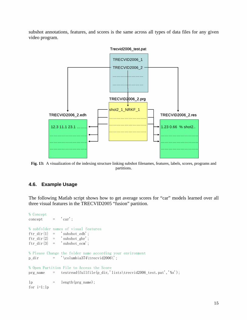
subshot annotations, features, and scores is the same across all types of data files for any given video program.

TRECVID2006_2

TRECVID2006_1

……………………

……………………

TRECVID2006_2.edh

12.3 11.1 23.1 ……..

………………………..

………………………..

………………………..

………………………..

………………………..

………………………..

Trecvid2006_test.pat

TRECVID2006_2.prg

1.23 0.66 % shot2..

………………………..

………………………..

………………………..

TRECVID2006_2.resshot2_1_NRKF_1

TRECVID2006_2

TRECVID2006_1

……………………

……………………

TRECVID2006_2.edh

12.3 11.1 23.1 ……..

………………………..

………………………..

………………………..

………………………..

………………………..

………………………..

Trecvid2006_test.pat

TRECVID2006_2.prg

1.23 0.66 % shot2..

………………………..

………………………..

………………………..

TRECVID2006_2.resshot2_1_NRKF_1

Fig. 13: A visualization of the indexing structure linking subshot filenames, features, labels, scores, programs and

partitions.

4.6. Example Usage The following Matlab script shows how to get average scores for “car” models learned over all three visual features in the TRECVID2005 “fusion” partition. % Concept concept = 'car'; % subfolder names of visual features ftr_dir{1} = 'subshot_edh'; ftr_dir{2} = 'subshot_gbr'; ftr_dir{3} = 'subshot_ecm'; % Please Change the folder name according your environment p_dir = '\columbia374\trecvid2006\'; % Open Partition File to Access the Score prg_name = textread(fullfile(p_dir,'lists\trecvid2006_test.pat','%s'); lp = length(prg_name); for i=1:lp

15

n_score = []; for j=1:3 % Make the feature file name with full path. score_file = fullfile(p_dir,'scores',concept,ftr_dir{j},[prg_name{i},'.res']); % Read only a normalized score n_t_score = textread(score_file,'*%f%f*%c*%s'); n_score = [n_score, n_t_score]; end % Take mean n_res = mean(n_score,2); % Store the result in xxx_tst.txt fid = fopen('test.txt','w'); lpj = length(n_res); for j=1:lpj fprintf(fid,'%f\n',n_res(j)); end fclose(fp); end

5. References [1] NIST, "TREC video retrieval evaluation (TRECVID)," 2001-2006.

[2] C. G. M. Snoek, M. Worring, J. C. v. Gemert, J.-M. Geusebroek, and A. W. M. Smeulders, "The challenge problem for automated detection of 101 semantic concepts in multimedia," in Proceedings of the 14th annual ACM international conference on Multimedia Santa Barbara, CA, USA 2006.

[3] S.-F. Chang, W. Hsu, L. Kennedy, L. Xie, A. Yanagawa, E. Zavesky, and D.-Q. Zhang, "Columbia University TRECVID-2005 Video Search and High-Level Feature Extraction," in NIST TRECVID workshop Gaithersburg, MD, 2005.

[4] S.-F. Chang, W. Jiang, W. Hsu, L. Kennedy, D. Xu, A. Yanagawa, and E. Zavesky, "Columbia University TRECVID-2006 Video Search and High-Level Feature Extraction," in NIST TRECVID workshop Gaithersburg, MD, 2006.

[5] "LSCOM Lexicon Definitions and Annotations Version 1.0, DTO Challenge Workshop on Large Scale Concept Ontology for Multimedia," Columbia University ADVENT Technical Report #217-2006-3, March 2006. Data set download site: http://www.ee.columbia.edu/dvmm/lscom/

[6] M. Naphade, J. R. Smith, J. Tesic, S.-F. Chang, W. Hsu, L. Kennedy, A. Hauptmann, J. Curtis, "Large-Scale Concept Ontology for Multimedia," IEEE Multimedia Magazine, 13(3), 2006.

[7] C.-C. Chang and C.-J. Lin, "LIBSVM: a Library for Support Vector Machines," 2001.

[8] A. Amir, J. Argillander, M. Campbell, A. Haubold, G. Iyengar, S. Ebadollahi, F. Kang, M. R. Naphade A. P. Natsev, John R. Smith, J. Tesic, and T. Volkmer, "IBM Research TRECVID-2005 Video Retrieval System," in NIST TRECVID workshop Gaithersburg, MD, 2005.

[9] C. Petersohn, "Fraunhofer HHI at TRECVID 2004: Shot Boundary Detection System," in TREC Video Retrieval Evaluation Online Proceedings: NIST, 2004.

[10] A. Yanagawa, W. Hsu, and S.-F. Chang, "Brief Descriptions of Visual Features for Baseline TRECVID Concept Detectors," Columbia University ADVENT Technical Report #219-2006-5, July 2006.

[11] B. L. Tseng, C.-Y. Lin, M. Naphade, A. Natsev, and J. R. Smith, "Normalized classifier fusion for semantic visual concept detection," in Proceedings of IEEE ICIP, 2003.

16

[12] J. C. Platt, "Probabilistic Outputs for Support Vector Machines and Comparisons to Regularized Likelihood Methods," in Advances in Large Margin Classifiers, 1999.

[13] W. Jiang, S.-F. Chang, and A. C. Loui, "Context-Based Concept Fusion with Boosted Conditional Random Fields," in IEEE International Conference on Acoustics, Speech, and Signal Processing (ICASSP) Hawaii, USA, 2007.

[14] L. Kennedy and S.-F. Chang, "A Reranking Approach for Context-based Concept Fusion in Video Indexing and Retrieval," ACM International Conference on Image and Video Retrieval (CIVR), Amsterdam, July 2007.

[15] D. Xu and S.-F. Chang, "Visual Event Recognition in News Video Using Kernel Methods with Multi-Level Temporal Alignment," IEEE CVPR, Minneapolis, June 2007.

17