Colorization as a Proxy Task for Visual Understanding · 2017-08-15 · Colorization as a Proxy...
10
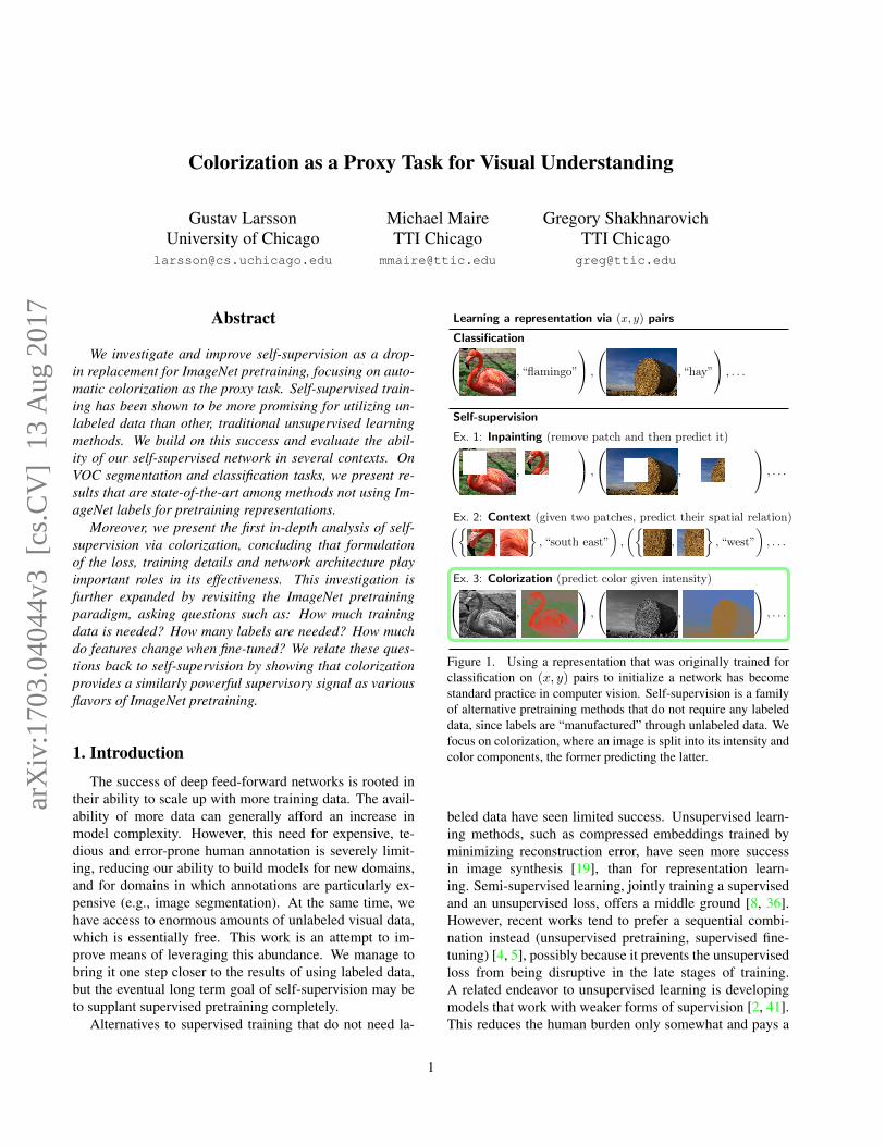
Colorization as a Proxy Task for Visual Understanding Gustav Larsson University of Chicago [email protected] Michael Maire TTI Chicago [email protected] Gregory Shakhnarovich TTI Chicago [email protected] Abstract We investigate and improve self-supervision as a drop- in replacement for ImageNet pretraining, focusing on auto- matic colorization as the proxy task. Self-supervised train- ing has been shown to be more promising for utilizing un- labeled data than other, traditional unsupervised learning methods. We build on this success and evaluate the abil- ity of our self-supervised network in several contexts. On VOC segmentation and classification tasks, we present re- sults that are state-of-the-art among methods not using Im- ageNet labels for pretraining representations. Moreover, we present the first in-depth analysis of self- supervision via colorization, concluding that formulation of the loss, training details and network architecture play important roles in its effectiveness. This investigation is further expanded by revisiting the ImageNet pretraining paradigm, asking questions such as: How much training data is needed? How many labels are needed? How much do features change when fine-tuned? We relate these ques- tions back to self-supervision by showing that colorization provides a similarly powerful supervisory signal as various flavors of ImageNet pretraining. 1. Introduction The success of deep feed-forward networks is rooted in their ability to scale up with more training data. The avail- ability of more data can generally afford an increase in model complexity. However, this need for expensive, te- dious and error-prone human annotation is severely limit- ing, reducing our ability to build models for new domains, and for domains in which annotations are particularly ex- pensive (e.g., image segmentation). At the same time, we have access to enormous amounts of unlabeled visual data, which is essentially free. This work is an attempt to im- prove means of leveraging this abundance. We manage to bring it one step closer to the results of using labeled data, but the eventual long term goal of self-supervision may be to supplant supervised pretraining completely. Alternatives to supervised training that do not need la- Learning a representation via (x, y) pairs Classification , “flamingo” , , “hay” ,... Self-supervision Ex. 1: Inpainting (remove patch and then predict it) , , , ,... Ex. 2: Context (given two patches, predict their spatial relation) , , “south east” , , , “west” ,... Ex. 3: Colorization (predict color given intensity) , , , ,... Figure 1. Using a representation that was originally trained for classification on (x, y) pairs to initialize a network has become standard practice in computer vision. Self-supervision is a family of alternative pretraining methods that do not require any labeled data, since labels are “manufactured” through unlabeled data. We focus on colorization, where an image is split into its intensity and color components, the former predicting the latter. beled data have seen limited success. Unsupervised learn- ing methods, such as compressed embeddings trained by minimizing reconstruction error, have seen more success in image synthesis [19], than for representation learn- ing. Semi-supervised learning, jointly training a supervised and an unsupervised loss, offers a middle ground [8, 36]. However, recent works tend to prefer a sequential combi- nation instead (unsupervised pretraining, supervised fine- tuning) [4, 5], possibly because it prevents the unsupervised loss from being disruptive in the late stages of training. A related endeavor to unsupervised learning is developing models that work with weaker forms of supervision [2, 41]. This reduces the human burden only somewhat and pays a 1 arXiv:1703.04044v3 [cs.CV] 13 Aug 2017
Transcript of Colorization as a Proxy Task for Visual Understanding · 2017-08-15 · Colorization as a Proxy...
Colorization as a Proxy Task for Visual Understanding
Gustav LarssonUniversity of Chicago
Michael MaireTTI Chicago
Gregory ShakhnarovichTTI [email protected]
Abstract
We investigate and improve self-supervision as a drop-in replacement for ImageNet pretraining, focusing on auto-matic colorization as the proxy task. Self-supervised train-ing has been shown to be more promising for utilizing un-labeled data than other, traditional unsupervised learningmethods. We build on this success and evaluate the abil-ity of our self-supervised network in several contexts. OnVOC segmentation and classification tasks, we present re-sults that are state-of-the-art among methods not using Im-ageNet labels for pretraining representations.
Moreover, we present the first in-depth analysis of self-supervision via colorization, concluding that formulationof the loss, training details and network architecture playimportant roles in its effectiveness. This investigation isfurther expanded by revisiting the ImageNet pretrainingparadigm, asking questions such as: How much trainingdata is needed? How many labels are needed? How muchdo features change when fine-tuned? We relate these ques-tions back to self-supervision by showing that colorizationprovides a similarly powerful supervisory signal as variousflavors of ImageNet pretraining.
1. IntroductionThe success of deep feed-forward networks is rooted in
their ability to scale up with more training data. The avail-ability of more data can generally afford an increase inmodel complexity. However, this need for expensive, te-dious and error-prone human annotation is severely limit-ing, reducing our ability to build models for new domains,and for domains in which annotations are particularly ex-pensive (e.g., image segmentation). At the same time, wehave access to enormous amounts of unlabeled visual data,which is essentially free. This work is an attempt to im-prove means of leveraging this abundance. We manage tobring it one step closer to the results of using labeled data,but the eventual long term goal of self-supervision may beto supplant supervised pretraining completely.
Alternatives to supervised training that do not need la-
Learning a representation via (x, y) pairs
Classification , “flamingo”
,
, “hay”
, . . .
Self-supervision
Ex. 1: Inpainting (remove patch and then predict it) ,
,
,
, . . .
Ex. 2: Context (given two patches, predict their spatial relation)({,
}, “south east”
),
({,
}, “west”
), . . .
Ex. 3: Colorization (predict color given intensity) ,
,
,
, . . .
Figure 1. Using a representation that was originally trained forclassification on (x, y) pairs to initialize a network has becomestandard practice in computer vision. Self-supervision is a familyof alternative pretraining methods that do not require any labeleddata, since labels are “manufactured” through unlabeled data. Wefocus on colorization, where an image is split into its intensity andcolor components, the former predicting the latter.
beled data have seen limited success. Unsupervised learn-ing methods, such as compressed embeddings trained byminimizing reconstruction error, have seen more successin image synthesis [19], than for representation learn-ing. Semi-supervised learning, jointly training a supervisedand an unsupervised loss, offers a middle ground [8, 36].However, recent works tend to prefer a sequential combi-nation instead (unsupervised pretraining, supervised fine-tuning) [4, 5], possibly because it prevents the unsupervisedloss from being disruptive in the late stages of training.A related endeavor to unsupervised learning is developingmodels that work with weaker forms of supervision [2, 41].This reduces the human burden only somewhat and pays a
1
arX
iv:1
703.
0404
4v3
[cs
.CV
] 1
3 A
ug 2
017
price in model performance.Recently, self-supervision has emerged as a new flavor of
unsupervised learning [4, 39]. The key observation is thatperhaps part of the benefit of labeled data is that it leadsto using a discriminative loss. This type of loss may bebetter suited for representation learning than, for instance,a reconstruction or likelihood-based loss. Self-supervisionis a way to use a discriminative loss on unlabeled data bypartitioning each input sample in two, predicting the parts’association. We focus on self-supervised colorization [21,43], where each image is split into its intensity and its color,using the former to predict the latter.
Our main contributions to self-supervision are:
• State-of-the-art results on VOC 2007 Classificationand VOC 2012 Segmentation, among methods that donot use ImageNet labels.
• The first in-depth analysis of self-supervision via col-orization. We study the impact of loss, network ar-chitecture and training details, showing that there aremany important aspects that influence results.
• An empirical study of various formulations of Im-ageNet pretraining and how they compare to self-supervision.
2. Related workIn our work on replacing classification-based pretrain-
ing for downstream supervised tasks, the first thing to con-sider is clever network initializations. Networks that are ini-tialized to promote uniform scale of activations across lay-ers, converge more easily and faster [7, 10]. The uniformscale however is only statistically predicted given broaddata assumptions, so this idea can be taken one step fur-ther by looking at the activations of actual data and normal-izing [24]. Using some training data to initialize weightsblurs the line between initialization and unsupervised pre-training. For instance, using layer-wise k-means cluster-ing [3, 20] should be considered unsupervised pretraining,even though it may be a particularly fast one.
Unsupervised pretraining can be used to facilitate op-timization or to expose the network to orders of magni-tude larger unlabeled data. The former was once a popu-lar motivation, but fell out of favor as it was made unnec-essary by improved training techniques (e.g. introductionof non-saturating activations [28], better initialization [7]and training algorithms [33, 18]). The second motivation ofleveraging more data, which can also be realized as semi-supervised training, is an open problem with current bestmethods rarely used in competitive vision systems.
Recent methods on self-supervised feature learning haveseen several incarnations, broadly divided into methods thatexploit temporal or spatial structure in natural visual data:
Temporal. There have been a wide variety of meth-ods that use the correlation between adjacent video framesas a learning signal. One way is to try to predict futureframes, which is an analogous task to language model-ing and often uses similar techniques based on RNNs andLSTMs [37, 34]. It is also possible to train an embed-ding where temporally close frames are considered similar(using either pairs [26, 15, 16] or triplets [39]). Anothermethod that uses a triplet loss presents three frames andtries to predict if they are correctly ordered [25]. Pathak etal. [31] learn general-purpose representation by predictingsaliency based on optical flow. Owens et al. [30], some-what breaking from the temporal category, operate on a sin-gle video frame to predict a statistical summary of the audiofrom the entire clip. The first video-based self-supervisionmethods were based on Independent Component Analysis(ICA) [38, 11]. Recent follow-up work generalizes this to anonlinear setting [12].
Spatial. Methods that operate on single-frame input typ-ically use the spatial dimensions to divide samples for self-supervision. Given a pair of patches from an image, Do-erch et al. [4] train representations by predicting which ofeight possible spatial compositions the two patches have.Noroozi & Favaro [29] take this further and learns a rep-resentation by solving a 3-by-3 jigsaw puzzle. The task ofinpainting (remove some pixels, then predict them) is uti-lized for representation learning by Pathak et al. [32]. Therehas also been work on using bi-directional Generative Ad-versarial Networks (BiGAN) to learn representations [5, 6].This is not what we typically regard as self-supervision, butit does similarly pose a supervised learning task (real vs.synthetic) on unlabeled data to drive representation learn-ing.
Colorization. Lastly there is colorization [21, 43, 44].Broadly speaking, the two previous categories split inputsamples along a spatio-temporal line, either predicting onegiven the other or predicting the line itself. Automatic col-orization departs from this as it asks to predict color over thesame pixel as its center of input, without discarding any spa-tial information. We speculate that this may make it moresuitable to tasks of similar nature, such as semantic segmen-tation; we demonstrate strong results on this benchmark.
Representation learning via colorization was first pre-sented as part of two automatic colorization papers [21, 43].Zhang et al. [43] present results across all PASCAL tasksand show colorization as a front-runner of self-supervision.However, like most self-supervision papers, it is restrictedto AlexNet and thus shows modest results compared to re-cent supervised methods. Larsson et al. [21] present state-of-the-art results on PASCAL VOC semantic segmenta-tion, which we improve by almost 10 points from 50.2%to 60.0% mIU. Both papers present the results with littleanalysis or investigation.
2
Dog Dog
ρ = .68
Athlete Athlete
.56Building Dome/Building
.42Monitor TV/Monitor
.28Red Car
.17Jack-o’-lantern Dog
.12
Before fine-tuning After fine-tuning
Fea
ture
sta
bili
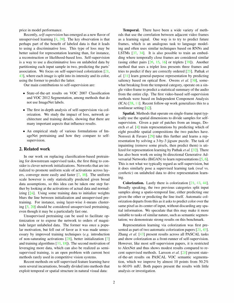
ty
Figure 2. Feature reuse/repurpose. The left column visualizestop activations from the colorization network (same as in Fig. 5).The right column visualizes the corresponding feature after thenetwork has been fine-tuned for semantic segmentation. Featuresare either re-used as is (top), specialized (middle), or scrapped andreplaced (bottom). See Fig. 3 for a quantitative study.
conv1_1 conv2_1 conv3_1 conv4_1 conv5_1 fc6 fc70.0
0.2
0.4
0.6
0.8
1.0
Corr
ela
tion m
edia
n
Col. Cls.
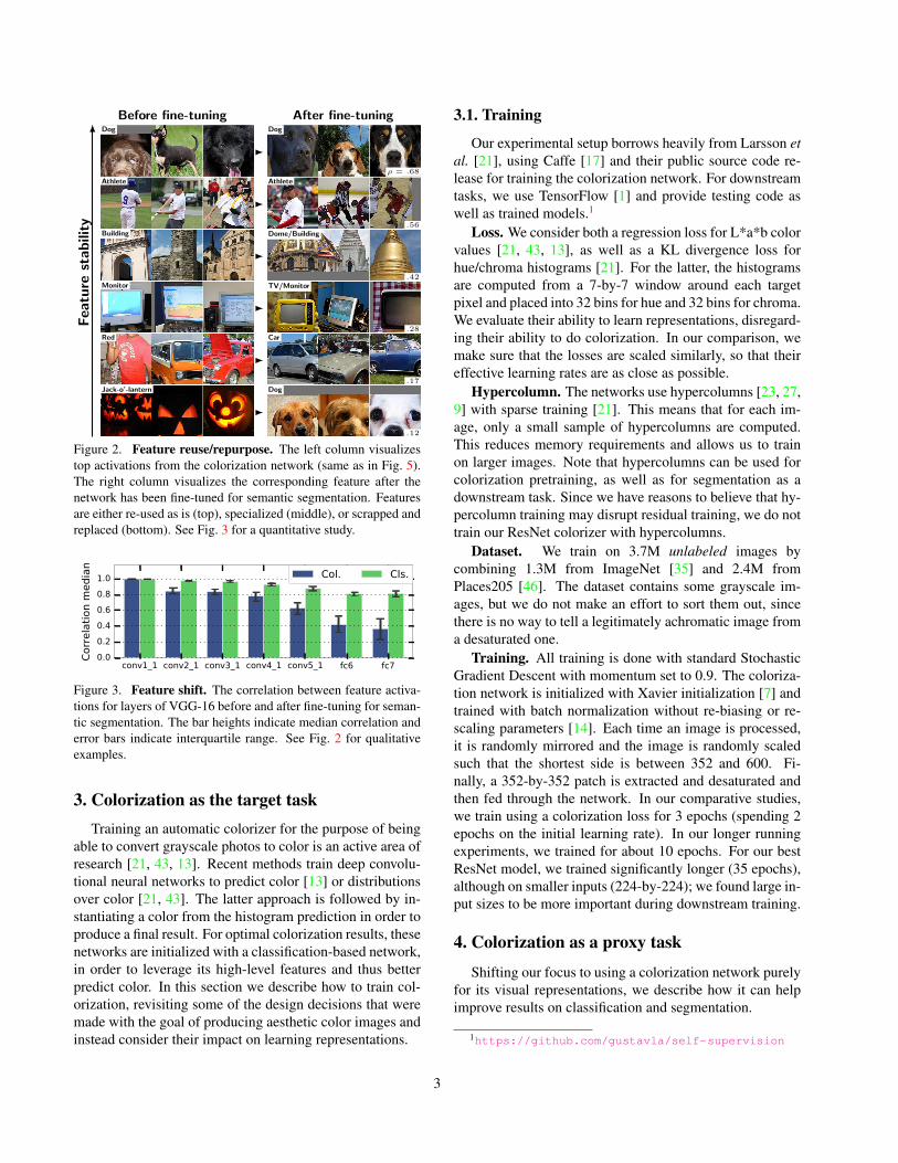
Figure 3. Feature shift. The correlation between feature activa-tions for layers of VGG-16 before and after fine-tuning for seman-tic segmentation. The bar heights indicate median correlation anderror bars indicate interquartile range. See Fig. 2 for qualitativeexamples.
3. Colorization as the target taskTraining an automatic colorizer for the purpose of being
able to convert grayscale photos to color is an active area ofresearch [21, 43, 13]. Recent methods train deep convolu-tional neural networks to predict color [13] or distributionsover color [21, 43]. The latter approach is followed by in-stantiating a color from the histogram prediction in order toproduce a final result. For optimal colorization results, thesenetworks are initialized with a classification-based network,in order to leverage its high-level features and thus betterpredict color. In this section we describe how to train col-orization, revisiting some of the design decisions that weremade with the goal of producing aesthetic color images andinstead consider their impact on learning representations.
3.1. Training
Our experimental setup borrows heavily from Larsson etal. [21], using Caffe [17] and their public source code re-lease for training the colorization network. For downstreamtasks, we use TensorFlow [1] and provide testing code aswell as trained models.1
Loss. We consider both a regression loss for L*a*b colorvalues [21, 43, 13], as well as a KL divergence loss forhue/chroma histograms [21]. For the latter, the histogramsare computed from a 7-by-7 window around each targetpixel and placed into 32 bins for hue and 32 bins for chroma.We evaluate their ability to learn representations, disregard-ing their ability to do colorization. In our comparison, wemake sure that the losses are scaled similarly, so that theireffective learning rates are as close as possible.
Hypercolumn. The networks use hypercolumns [23, 27,9] with sparse training [21]. This means that for each im-age, only a small sample of hypercolumns are computed.This reduces memory requirements and allows us to trainon larger images. Note that hypercolumns can be used forcolorization pretraining, as well as for segmentation as adownstream task. Since we have reasons to believe that hy-percolumn training may disrupt residual training, we do nottrain our ResNet colorizer with hypercolumns.
Dataset. We train on 3.7M unlabeled images bycombining 1.3M from ImageNet [35] and 2.4M fromPlaces205 [46]. The dataset contains some grayscale im-ages, but we do not make an effort to sort them out, sincethere is no way to tell a legitimately achromatic image froma desaturated one.
Training. All training is done with standard StochasticGradient Descent with momentum set to 0.9. The coloriza-tion network is initialized with Xavier initialization [7] andtrained with batch normalization without re-biasing or re-scaling parameters [14]. Each time an image is processed,it is randomly mirrored and the image is randomly scaledsuch that the shortest side is between 352 and 600. Fi-nally, a 352-by-352 patch is extracted and desaturated andthen fed through the network. In our comparative studies,we train using a colorization loss for 3 epochs (spending 2epochs on the initial learning rate). In our longer runningexperiments, we trained for about 10 epochs. For our bestResNet model, we trained significantly longer (35 epochs),although on smaller inputs (224-by-224); we found large in-put sizes to be more important during downstream training.
4. Colorization as a proxy task
Shifting our focus to using a colorization network purelyfor its visual representations, we describe how it can helpimprove results on classification and segmentation.
1https://github.com/gustavla/self-supervision
3
4.1. Training
The downstream task is trained by initializing weightsfrom the colorization-from-scratch network. Some key con-siderations follow:
Early stopping. Training on a small sample size is proneto overfitting. We have found that the most effective methodof preventing this is carefully cross validating the learningrate schedule. Models that initialize differently (random,colorization, classification), need very different early stop-ping schedules. Finding a method that works well in allthese settings was key to our study. We split the trainingdata 90/10 and only train on the 90%; the rest is used tomonitor overfitting. Each time the 10% validation score(not surrogate loss) stops improving, the learning rate isdropped. After this is done twice, the training is concluded.For our most competitive experiments (Tab. 1), we then re-train using 100% of the data with the cross-validated learn-ing rate schedule fixed.
Receptive field. Previous work on semantic segmenta-tion has shown the importance of large receptive fields [27,42]. One way of accomplishing this is by using dilatedconvolutions [42, 40], however this redefines the interpre-tation of filters and thus requires re-training. Instead, weadd two additional blocks (2-by-2 max pooling of stride 2,3-by-3 convolution with 1,024 features) at the top of thenetwork, each expanding the receptive field with 160 pixelsper block. We train on large input images (448-by-448) inorder to fully appreciate the enlarged receptive field.
Hypercolumn. Note that using a hypercolumn when thedownstream task is semantic segmentation is a separate de-sign choice that does not need to be coupled with the useof hypercolumns during colorization pretraining. In eithercase, the post-hypercolumn parameter weights are never re-used. For ResNet, we use a subset of the full hypercolumn.2
Batch normalization. The models trained from scratchuse parameter-free batch normalization. However, fordownstream training, we absorb the mean and variance intothe weights and biases and train without batch normaliza-tion (with the exception of ResNet, where in our experienceit helps). For networks that were not trained with batch nor-malization and are not well-balanced in scale across layers(e.g. ImageNet pretrained VGG-16), we re-balance the net-work so that each layer’s activation has unit variance [21].
Padding. For our ImageNet pretraining experiments,we observe that going from a classification network to afully convolutional network can introduce edge effects dueto each layer’s zero padding. A problem not exhibited bythe original VGG-16, leading us to suspect that it may bedue to the introduction of batch normalization. For thenewly trained networks, activations increase close to the
2ResNet-152 hypercolumn: conv1, res2{a,b,c},res3b{1,4,7}, res4b{5,10,15,20,25,30,35}, res5c
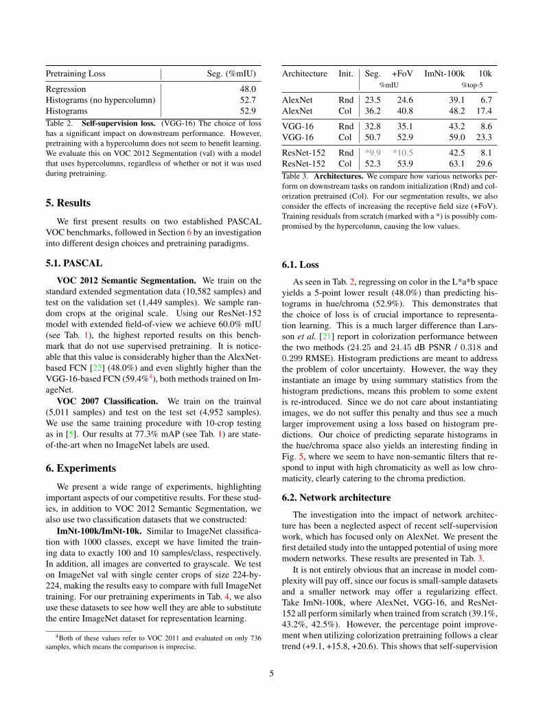
Initialization Architecture Class. Seg.%mAP %mIU
ImageNet (+FoV) VGG-16 86.9 69.5
Random (ours) AlexNet 46.2 23.5Random [32] AlexNet 53.3 19.8k-means [20, 5] AlexNet 56.6 32.6k-means [20] VGG-16 56.5 -k-means [20] GoogLeNet 55.0 -
Pathak et al. [32] AlexNet 56.5 29.7Wang & Gupta [39] AlexNet 58.7 -Donahue et al. [5] AlexNet 60.1 35.2Doersch et al. [4, 5] AlexNet 65.3 -Zhang et al. (col) [43] AlexNet 65.6 35.6Zhang et al. (s-b) [44] AlexNet 67.1 36.0Noroozi & Favaro [29] Mod. AlexNet 68.6 -Larsson et al. [21] VGG-16 - 50.2
Our method AlexNet 65.9 38.4(+FoV) VGG-16 77.2 56.0(+FoV) ResNet-152 77.3 60.0
Table 1. VOC Comparison. Comparison with other initializa-tion and self-supervision methods on VOC 2007 Classification(test) and VOC 2012 Segmentation (val). Note that our base-line AlexNet results (38.4%) are also the most competitive amongAlexNet models. The use of a hypercolumn instead of FCNis partly responsible: running Zhang et al.’s colorization modelwith a hypercolumn yields 36.4%, only a slight improvement over35.6%. Switching to ResNet, adding a larger FoV, and trainingeven longer yields a significantly higher result at 60.0% mIU.Note, the “+FoV” only affects the segmentation results. The mod-ified AlexNet used by Noroozi & Favaro has the same number ofparameters as AlexNet, with a spatial reduction of 2 moved fromconv1 to pool5, increasing the size of the intermediate activations.
edge, even though the receptive fields increasingly hangover the edge of the image, reducing the amount of seman-tic information. Correcting for this3 makes activations well-behaved, which was important in order to appropriately vi-sualize top activations. However, it does not offer a measur-able improvement on downstream tasks, which means thenetwork can correct for this during the fine-tuning stage.
Color. Since the domain of a colorization networkis grayscale, our downstream experiments operate ongrayscale input unless otherwise stated. When coloriza-tion is re-introduced, we convert the grayscale filters inconv1 1 to RGB (replicate to all three channels, divideby three) and let them fine-tune on the downstream task.
3We pad with the bias from the previous layer, instead of with zeros.This is an estimate of the expectation value, since we use a parameter-freebatch normalization with zero mean, leaving only the bias.
4
Pretraining Loss Seg. (%mIU)
Regression 48.0Histograms (no hypercolumn) 52.7Histograms 52.9Table 2. Self-supervision loss. (VGG-16) The choice of losshas a significant impact on downstream performance. However,pretraining with a hypercolumn does not seem to benefit learning.We evaluate this on VOC 2012 Segmentation (val) with a modelthat uses hypercolumns, regardless of whether or not it was usedduring pretraining.
5. Results
We first present results on two established PASCALVOC benchmarks, followed in Section 6 by an investigationinto different design choices and pretraining paradigms.
5.1. PASCAL
VOC 2012 Semantic Segmentation. We train on thestandard extended segmentation data (10,582 samples) andtest on the validation set (1,449 samples). We sample ran-dom crops at the original scale. Using our ResNet-152model with extended field-of-view we achieve 60.0% mIU(see Tab. 1), the highest reported results on this bench-mark that do not use supervised pretraining. It is notice-able that this value is considerably higher than the AlexNet-based FCN [22] (48.0%) and even slightly higher than theVGG-16-based FCN (59.4%4), both methods trained on Im-ageNet.
VOC 2007 Classification. We train on the trainval(5,011 samples) and test on the test set (4,952 samples).We use the same training procedure with 10-crop testingas in [5]. Our results at 77.3% mAP (see Tab. 1) are state-of-the-art when no ImageNet labels are used.
6. Experiments
We present a wide range of experiments, highlightingimportant aspects of our competitive results. For these stud-ies, in addition to VOC 2012 Semantic Segmentation, wealso use two classification datasets that we constructed:
ImNt-100k/ImNt-10k. Similar to ImageNet classifica-tion with 1000 classes, except we have limited the train-ing data to exactly 100 and 10 samples/class, respectively.In addition, all images are converted to grayscale. We teston ImageNet val with single center crops of size 224-by-224, making the results easy to compare with full ImageNettraining. For our pretraining experiments in Tab. 4, we alsouse these datasets to see how well they are able to substitutethe entire ImageNet dataset for representation learning.
4Both of these values refer to VOC 2011 and evaluated on only 736samples, which means the comparison is imprecise.
Architecture Init. Seg. +FoV ImNt-100k 10k%mIU %top-5
AlexNet Rnd 23.5 24.6 39.1 6.7AlexNet Col 36.2 40.8 48.2 17.4
VGG-16 Rnd 32.8 35.1 43.2 8.6VGG-16 Col 50.7 52.9 59.0 23.3
ResNet-152 Rnd *9.9 *10.5 42.5 8.1ResNet-152 Col 52.3 53.9 63.1 29.6Table 3. Architectures. We compare how various networks per-form on downstream tasks on random initialization (Rnd) and col-orization pretrained (Col). For our segmentation results, we alsoconsider the effects of increasing the receptive field size (+FoV).Training residuals from scratch (marked with a *) is possibly com-promised by the hypercolumn, causing the low values.
6.1. Loss
As seen in Tab. 2, regressing on color in the L*a*b spaceyields a 5-point lower result (48.0%) than predicting his-tograms in hue/chroma (52.9%). This demonstrates thatthe choice of loss is of crucial importance to representa-tion learning. This is a much larger difference than Lars-son et al. [21] report in colorization performance betweenthe two methods (24.25 and 24.45 dB PSNR / 0.318 and0.299 RMSE). Histogram predictions are meant to addressthe problem of color uncertainty. However, the way theyinstantiate an image by using summary statistics from thehistogram predictions, means this problem to some extentis re-introduced. Since we do not care about instantiatingimages, we do not suffer this penalty and thus see a muchlarger improvement using a loss based on histogram pre-dictions. Our choice of predicting separate histograms inthe hue/chroma space also yields an interesting finding inFig. 5, where we seem to have non-semantic filters that re-spond to input with high chromaticity as well as low chro-maticity, clearly catering to the chroma prediction.
6.2. Network architecture
The investigation into the impact of network architec-ture has been a neglected aspect of recent self-supervisionwork, which has focused only on AlexNet. We present thefirst detailed study into the untapped potential of using moremodern networks. These results are presented in Tab. 3.
It is not entirely obvious that an increase in model com-plexity will pay off, since our focus is small-sample datasetsand a smaller network may offer a regularizing effect.Take ImNt-100k, where AlexNet, VGG-16, and ResNet-152 all perform similarly when trained from scratch (39.1%,43.2%, 42.5%). However, the percentage point improve-ment when utilizing colorization pretraining follows a cleartrend (+9.1, +15.8, +20.6). This shows that self-supervision
5

Pretraining Samples Epochs Seg. (%mIU)
None - - 35.1
C1000 1.3M 80 66.5C1000 1.3M 20 62.0C1000 100k 250 57.1C1000 10k 250 44.4
E10 (1.17M) 1.3M 20 61.8E50 (0.65M) 1.3M 20 59.4
H16 1.3M 20 60.0H2 1.3M 20 46.1
R50 1.3M 20 57.340 59.4
R16 1.3M 20 42.640 53.5
Example: H3 (3 hierarchical label buckets)
Label #1 Label #2 Label #3
Example: R3 (3 random label buckets)
Label #1 Label #2 Label #3
Table 4. ImageNet pretraining. We evaluate how useful variousmodifications of ImageNet are for VOC 2012 Segmentation (val-gray). We create new datasets either by reducing sample size orby reducing the label space. The former is done simply by reduc-ing sample size or by introducing 10% (E10) or 50% (E50) labelnoise. The latter is done using hierarchical label buckets (H16 andH2) or random label buckets (R50 and R16). The model trainedfor 80 epochs is the publicly available VGG-16 (trained for 76epochs) that we fine-tuned for grayscale for 4 epochs. The rest ofthe models were trained from scratch on grayscale images.
allows us to benefit from higher model complexity even insmall-sample regimes. Compare this with k-means initial-ization [20], which does not show any improvements whenincreasing model complexity (Tab. 1).
Training ResNet from scratch for semantic segmentationis an outlier value in the table. This is the only experimentthat trains a residual network from scratch together with ahypercolumn; this could be a disruptive combination as thelow numbers suggest.
Initialization Grayscale input Color input
Classification 66.5 69.5Colorization 56.0 55.9Table 5. Color vs. Grayscale input. (VOC 2012 Segmentation,%mIU) Even though our classification-based model does 3 pointsbetter using color, re-introducing color yields no benefit.
6.3. ImageNet pretraining
We relate self-supervised pretraining to ImageNet pre-training by revisiting and reconsidering various aspects ofthis paradigm (see Tab. 4). First of all, we investigate theimportance of 1000 classes (C1000). To do this, we join Im-ageNet classes together based on their place in the WordNethierarchy, creating two new datasets with 16 classes (H16)and only two classes (H2). We show that H16 performsonly slightly short of C1000 on a downstream task with 21classes, while H2 is significantly worse. If we compare thisto our colorization pretraining, it is much better than H2 andonly slightly worse than H16.
Next, we study the impact of sample size, using thesubsets ImNt-100k and ImNt-10k described in Section 6.ImNt-100k does similarly well as self-supervised coloriza-tion (57.1% vs. 56.0% for VGG-16), suggesting that ourmethod has roughly replaced 0.1 million labeled sampleswith 3.7 million unlabeled samples. Reducing samples to10 per class sees a bigger drop in downstream results. Thisresult is similar to H2, which is somewhat surprising: col-lapsing the label space to a binary prediction is roughly asbad as using 1/100th of the training data. Recalling the im-provements going from regression to histogram predictionfor colorization, the richness of the label space seems criti-cal for representation learning.
We take the 1000 ImageNet classes and randomly placethem in 50 (R50) or 16 (R16) buckets that we dub our newlabels. This means that we are training a highly complexdecision boundary that may dictate that a golden retrieverand a minibus belong to the same label, but a golden re-triever and a border collie do not. We consider this analo-gous to self-supervised colorization, since the supervisorysignal similarly considers a red car arbitrarily more simi-lar to a red postbox than to a blue car. Not surprisingly,our contrived dataset R50 results in a 5-point drop on ourdownstream task, and R16 even more so with a 20-pointdrop. However, we noticed that the training loss was stillactively decreasing after 20 epochs. Training instead for 40epochs showed an improvement by about 2 points for R50,while 11 points for R16. In other words, complex classescan provide useful supervision for representation learning,but training may take longer. This is consistent with ourimpression of self-supervised colorization; although it con-verges slowly, it keeps improving its feature generality with
6
0.0 0.5 1.0 1.5 2.0 2.5 3.0 10.0
Epochs
2.2
2.3
2.4
2.5
2.6
2.7
2.8
2.9
Tra
inin
g L
oss
Col.
30
35
40
45
50
55
60
65
%m
IU
Seg.
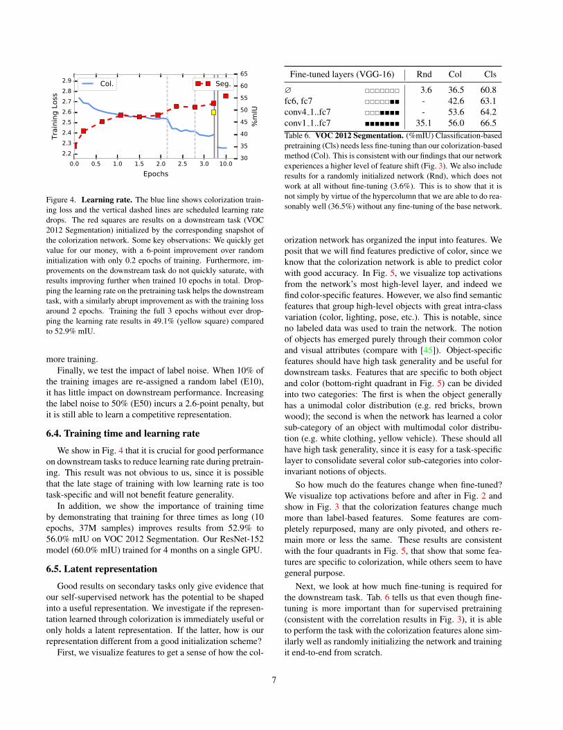
Figure 4. Learning rate. The blue line shows colorization train-ing loss and the vertical dashed lines are scheduled learning ratedrops. The red squares are results on a downstream task (VOC2012 Segmentation) initialized by the corresponding snapshot ofthe colorization network. Some key observations: We quickly getvalue for our money, with a 6-point improvement over randominitialization with only 0.2 epochs of training. Furthermore, im-provements on the downstream task do not quickly saturate, withresults improving further when trained 10 epochs in total. Drop-ping the learning rate on the pretraining task helps the downstreamtask, with a similarly abrupt improvement as with the training lossaround 2 epochs. Training the full 3 epochs without ever drop-ping the learning rate results in 49.1% (yellow square) comparedto 52.9% mIU.
more training.Finally, we test the impact of label noise. When 10% of
the training images are re-assigned a random label (E10),it has little impact on downstream performance. Increasingthe label noise to 50% (E50) incurs a 2.6-point penalty, butit is still able to learn a competitive representation.
6.4. Training time and learning rate
We show in Fig. 4 that it is crucial for good performanceon downstream tasks to reduce learning rate during pretrain-ing. This result was not obvious to us, since it is possiblethat the late stage of training with low learning rate is tootask-specific and will not benefit feature generality.
In addition, we show the importance of training timeby demonstrating that training for three times as long (10epochs, 37M samples) improves results from 52.9% to56.0% mIU on VOC 2012 Segmentation. Our ResNet-152model (60.0% mIU) trained for 4 months on a single GPU.
6.5. Latent representation
Good results on secondary tasks only give evidence thatour self-supervised network has the potential to be shapedinto a useful representation. We investigate if the represen-tation learned through colorization is immediately useful oronly holds a latent representation. If the latter, how is ourrepresentation different from a good initialization scheme?
First, we visualize features to get a sense of how the col-
Fine-tuned layers (VGG-16) Rnd Col Cls
∅ ������� 3.6 36.5 60.8fc6, fc7 ������� - 42.6 63.1conv4 1..fc7 ������� - 53.6 64.2conv1 1..fc7 ������� 35.1 56.0 66.5Table 6. VOC 2012 Segmentation. (%mIU) Classification-basedpretraining (Cls) needs less fine-tuning than our colorization-basedmethod (Col). This is consistent with our findings that our networkexperiences a higher level of feature shift (Fig. 3). We also includeresults for a randomly initialized network (Rnd), which does notwork at all without fine-tuning (3.6%). This is to show that it isnot simply by virtue of the hypercolumn that we are able to do rea-sonably well (36.5%) without any fine-tuning of the base network.
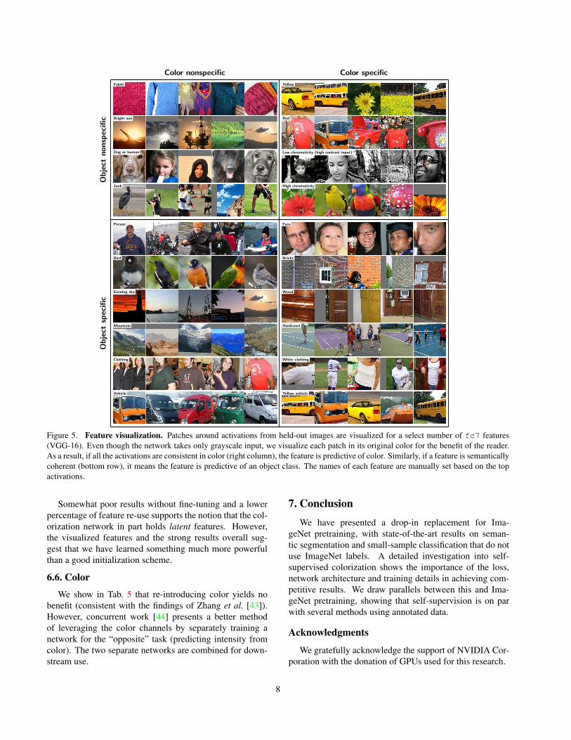
orization network has organized the input into features. Weposit that we will find features predictive of color, since weknow that the colorization network is able to predict colorwith good accuracy. In Fig. 5, we visualize top activationsfrom the network’s most high-level layer, and indeed wefind color-specific features. However, we also find semanticfeatures that group high-level objects with great intra-classvariation (color, lighting, pose, etc.). This is notable, sinceno labeled data was used to train the network. The notionof objects has emerged purely through their common colorand visual attributes (compare with [45]). Object-specificfeatures should have high task generality and be useful fordownstream tasks. Features that are specific to both objectand color (bottom-right quadrant in Fig. 5) can be dividedinto two categories: The first is when the object generallyhas a unimodal color distribution (e.g. red bricks, brownwood); the second is when the network has learned a colorsub-category of an object with multimodal color distribu-tion (e.g. white clothing, yellow vehicle). These should allhave high task generality, since it is easy for a task-specificlayer to consolidate several color sub-categories into color-invariant notions of objects.
So how much do the features change when fine-tuned?We visualize top activations before and after in Fig. 2 andshow in Fig. 3 that the colorization features change muchmore than label-based features. Some features are com-pletely repurposed, many are only pivoted, and others re-main more or less the same. These results are consistentwith the four quadrants in Fig. 5, that show that some fea-tures are specific to colorization, while others seem to havegeneral purpose.
Next, we look at how much fine-tuning is required forthe downstream task. Tab. 6 tells us that even though fine-tuning is more important than for supervised pretraining(consistent with the correlation results in Fig. 3), it is ableto perform the task with the colorization features alone sim-ilarly well as randomly initializing the network and trainingit end-to-end from scratch.
7
Fabric
Bright sun
Dog or human
Junk
Yellow
Red
Low chromaticity (high contrast input)
High chromaticity
Person
Bird
Evening sky
Mountain
Clothing
Vehicle
Face
Bricks
Wood
Hardcourt
White clothing
Yellow vehicle
Color nonspecific Color specific
Ob
ject
no
nsp
ecifi
cO
bje
ctsp
ecifi
c
Figure 5. Feature visualization. Patches around activations from held-out images are visualized for a select number of fc7 features(VGG-16). Even though the network takes only grayscale input, we visualize each patch in its original color for the benefit of the reader.As a result, if all the activations are consistent in color (right column), the feature is predictive of color. Similarly, if a feature is semanticallycoherent (bottom row), it means the feature is predictive of an object class. The names of each feature are manually set based on the topactivations.
Somewhat poor results without fine-tuning and a lowerpercentage of feature re-use supports the notion that the col-orization network in part holds latent features. However,the visualized features and the strong results overall sug-gest that we have learned something much more powerfulthan a good initialization scheme.
6.6. Color
We show in Tab. 5 that re-introducing color yields nobenefit (consistent with the findings of Zhang et al. [43]).However, concurrent work [44] presents a better methodof leveraging the color channels by separately training anetwork for the “opposite” task (predicting intensity fromcolor). The two separate networks are combined for down-stream use.
7. Conclusion
We have presented a drop-in replacement for Ima-geNet pretraining, with state-of-the-art results on seman-tic segmentation and small-sample classification that do notuse ImageNet labels. A detailed investigation into self-supervised colorization shows the importance of the loss,network architecture and training details in achieving com-petitive results. We draw parallels between this and Ima-geNet pretraining, showing that self-supervision is on parwith several methods using annotated data.
Acknowledgments
We gratefully acknowledge the support of NVIDIA Cor-poration with the donation of GPUs used for this research.
8

References[1] TensorFlow: Large-scale machine learning on heteroge-
neous systems, 2015. Software available from tensor-flow.org. 3
[2] A. Bearman, O. Russakovsky, V. Ferrari, and L. Fei-Fei.What’s the Point: Semantic Segmentation with Point Super-vision. In ECCV, 2016. 1
[3] A. Coates, H. Lee, and A. Y. Ng. An analysis of single-layer networks in unsupervised feature learning. In AISTATS,2011. 2
[4] C. Doersch, A. Gupta, and A. A. Efros. Unsupervised vi-sual representation learning by context prediction. In ICCV,2015. 1, 2, 4
[5] J. Donahue, P. Krahenbuhl, and T. Darrell. Adversarial fea-ture learning. In ICLR, 2017. 1, 2, 4, 5
[6] V. Dumoulin, I. Belghazi, B. Poole, A. Lamb, M. Arjovsky,O. Mastropietro, and A. Courville. Adversarially learned in-ference. arXiv preprint arXiv:1606.00704, 2016. 2
[7] X. Glorot and Y. Bengio. Understanding the difficulty oftraining deep feedforward neural networks. In AISTATS,2010. 2, 3
[8] Y. Grandvalet and Y. Bengio. Semi-supervised learning byentropy minimization. In NIPS, 2004. 1
[9] B. Hariharan, P. A. an R. Girshick, and J. Malik. Hyper-columns for object segmentation and fine-grained localiza-tion. CVPR, 2015. 3
[10] K. He, X. Zhang, S. Ren, and J. Sun. Delving deep intorectifiers: Surpassing human-level performance on imagenetclassification. CoRR, abs/1502.01852, 2015. 2
[11] J. Hurri and A. Hyvarinen. Simple-cell-like receptive fieldsmaximize temporal coherence in natural video. Neural Com-putation, 15(3):663–691, 2003. 2
[12] A. Hyvarinen and H. Morioka. Unsupervised feature extrac-tion by time-contrastive learning and nonlinear ica. In NIPS,2016. 2
[13] S. Iizuka, E. Simo-Serra, and H. Ishikawa. Let there beColor!: Joint End-to-end Learning of Global and Local Im-age Priors for Automatic Image Colorization with Simulta-neous Classification. ACM Transactions on Graphics (Proc.of SIGGRAPH 2016), 35(4), 2016. 3
[14] S. Ioffe and C. Szegedy. Batch normalization: Acceleratingdeep network training by reducing internal covariate shift. InICML, 2015. 3
[15] P. Isola, D. Zoran, D. Krishnan, and E. H. Adelson. Learningvisual groups from co-occurrences in space and time. arXivpreprint arXiv:1511.06811, 2015. 2
[16] D. Jayaraman and K. Grauman. Slow and steady featureanalysis: higher order temporal coherence in video. InCVPR, 2016. 2
[17] Y. Jia, E. Shelhamer, J. Donahue, S. Karayev, J. Long, R. Gir-shick, S. Guadarrama, and T. Darrell. Caffe: Convolu-tional architecture for fast feature embedding. arXiv preprintarXiv:1408.5093, 2014. 3
[18] D. P. Kingma and J. Ba. Adam: A method for stochasticoptimization. In ICLR, 2015. 2
[19] D. P. Kingma and M. Welling. Auto-encoding variationalbayes. In ICLR, 2014. 1
[20] P. Krahenbuhl, C. Doersch, J. Donahue, and T. Darrell. Data-dependent initializations of convolutional neural networks.In ICLR, 2016. 2, 4, 6
[21] G. Larsson, M. Maire, and G. Shakhnarovich. Learning rep-resentations for automatic colorization. In ECCV, 2016. 2,3, 4, 5
[22] J. Long, E. Shelhamer, and T. Darrell. Fully convolutionalnetworks for semantic segmentation. In CVPR, 2015. 5
[23] M. Maire, S. X. Yu, and P. Perona. Reconstructive sparsecode transfer for contour detection and semantic labeling. InACCV, 2014. 3
[24] D. Mishkin and J. Matas. All you need is a good init. arXivpreprint arXiv:1511.06422, 2015. 2
[25] I. Misra, C. L. Zitnick, and M. Hebert. Unsupervised learn-ing using sequential verification for action recognition. 2016.2
[26] H. Mobahi, R. Collobert, and J. Weston. Deep learning fromtemporal coherence in video. In ICML, 2009. 2
[27] M. Mostajabi, P. Yadollahpour, and G. Shakhnarovich. Feed-forward semantic segmentation with zoom-out features. InCVPR, 2015. 3, 4
[28] V. Nair and G. E. Hinton. Rectified linear units improverestricted boltzmann machines. In ICML, pages 807–814,2010. 2
[29] M. Noroozi and P. Favaro. Unsupervised learning of visualrepresentations by solving jigsaw puzzles. In ECCV, 2016.2, 4
[30] A. Owens, J. Wu, J. H. McDermott, W. T. Freeman, andA. Torralba. Ambient sound provides supervision for visuallearning. In ECCV, 2016. 2
[31] D. Pathak, R. B. Girshick, P. Dollar, T. Darrell, and B. Hari-haran. Learning features by watching objects move. CoRR,abs/1612.06370, 2016. 2
[32] D. Pathak, P. Krahenbuhl, J. Donahue, T. Darrell, andA. Efros. Context encoders: Feature learning by inpainting.In CVPR, 2016. 2, 4
[33] N. Qian. On the momentum term in gradient descent learningalgorithms. Neural networks, 12(1):145–151, 1999. 2
[34] M. Ranzato, A. Szlam, J. Bruna, M. Mathieu, R. Collobert,and S. Chopra. Video (language) modeling: a baselinefor generative models of natural videos. arXiv preprintarXiv:1412.6604, 2014. 2
[35] O. Russakovsky, J. Deng, H. Su, J. Krause, S. Satheesh,S. Ma, Z. Huang, A. Karpathy, A. Khosla, M. Bernstein,A. C. Berg, and L. Fei-Fei. ImageNet Large Scale VisualRecognition Challenge. International Journal of ComputerVision (IJCV), 115(3), 2015. 3
[36] M. Sajjadi, M. Javanmardi, and T. Tasdizen. Regularizationwith stochastic transformations and perturbations for deepsemi-supervised learning. NIPS, 2016. 1
[37] N. Srivastava, E. Mansimov, and R. Salakhutdinov. Unsu-pervised learning of video representations using lstms. InICML, 2015. 2
[38] J. H. van Hateren and D. L. Ruderman. Independent com-ponent analysis of natural image sequences yields spatio-temporal filters similar to simple cells in primary visual cor-tex. Proceedings of the Royal Society of London B: Biologi-cal Sciences, 265(1412):2315–2320, 1998. 2
9
[39] X. Wang and A. Gupta. Unsupervised learning of visual rep-resentations using videos. In ICCV, 2015. 2, 4
[40] Z. Wu, C. Shen, and A. van den Hengel. High-performancesemantic segmentation using very deep fully convolutionalnetworks. CoRR, abs/1604.04339, 2016. 4
[41] J. Xu, A. G. Schwing, and R. Urtasun. Learning to segmentunder various forms of weak supervision. In CVPR, 2015. 1
[42] F. Yu and V. Koltun. Multi-scale context aggregation by di-lated convolutions. In ICLR, 2016. 4
[43] R. Zhang, P. Isola, and A. A. Efros. Colorful image coloriza-tion. In ECCV, 2016. 2, 3, 4, 8
[44] R. Zhang, P. Isola, and A. A. Efros. Split-brain autoen-coders: Unsupervised learning by cross-channel prediction.In CVPR, 2017. 2, 4, 8
[45] B. Zhou, A. Khosla, A. Lapedriza, A. Oliva, and A. Torralba.Object detectors emerge in deep scene cnns. In ICLR, 2015.7
[46] B. Zhou, A. Lapedriza, J. Xiao, A. Torralba, and A. Oliva.Learning deep features for scene recognition using placesdatabase. In NIPS, pages 487–495, 2014. 3
A. Document changelogOverview of document revisions:
v1 Initial release.
v2 CVPR 2017 camera-ready release. Updated ResNet-152 results in Tab. 1 due to additional training for VOC2007 Classification (76.9 → 77.3) and VOC 2012Segmentation (59.0 → 60.0). Added label noise ex-periments (E10, E50). Renamed C2/C16 to H2/H16.Added references to concurrent work.
v3 Added overlooked reference.
10