Colorado State UniversityFt. Collins, CO 80523

and

Institute for Computational StudiesP.O. Box 1852

Ft. Collins, CO 80522

(NASA-CR- 177020}-- R E M O T E ACCESS TOR MAS: H86-30370 •'•SUPESCOMPUTING IN A U N I V E R S I T Y ENVIRONMENTFinal Report, 1 Apr. , ,1S85 - 31 Har. ,1986(Colorado State Univ. ) 60 p CSCL 09B Unclas

G3/6 "

Remote Access for NAS: Supercomputing in a University Environment

Final Report, covering the period April 1, 1985 through March 31, 1986

Cooperative Agreement NCC2-344

Gary Johnson - Principal InvestigatorBecky OlsonJulie SwisshelmDan PryorJohn Ziebarth

https://ntrs.nasa.gov/search.jsp?R=19860020898 2020-03-28T23:59:27+00:00Z

The experiment was designed to assist the NAS (Numerical Aerodynamic Simulation)Project Office in the testing and evaluation of long haul communications for remoteusers. The objectives of this work were to:

(1) Use foreign workstations to remotely access the NAS system. In this way problems associated withinterfacing equipment commonly used by university and industrial investigators to the NAS facility canbe identified and solutions to these problems found.

(2) Provide NAS with a link to a large university-based computing facility which can serve as a modelfor a regional node of the Long-Haul Communications Subsystem (LHCS).

(3) Provide a tail circuit to the University of Colorado at Boulder thereby simulating the complete com-munications path from NAS through a regional node to an end-user.

To meet these objectives the Institute for Computational Studies (ICS) took deliveryof a Sun-2 160 color workstation in the first part of June. Another Sun-2 160 colorworkstation arrived in early July.

The first problem encountered by NAS/ICS was the inability of the Sun workstationto run a graphics software package (PLOT3D) available on NASA's Silicon GraphicsIRIS workstation. Becky Olson spent a week at NASA/Ames in May learning aboutthe graphics package and the IRIS. She spent the next month converting it to the SUNworkstation so the communication experiment could take place. The modified sourcecode for the Sun version of PLOT3D is listed in Appendix I.

The 56 kilobaud line and the data service unit were installed during the week of July29. By August 1, NASA/Ames and ICS were communicating through the 56 kilobaudline, providing NAS with a link to a university.

The next phase of the experiment was to determine if the 56 kilobaud line was ade-quate for actual development work and data and graphic file transfers. JulieSwisshelm spent the week of August 19 through 23 conducting Computational FluidDynamics (CFD) runs at NASA/Ames to have a base in determining the time it takesto run a CFD problem and transfer files locally at NASA Ames.

The next week (August 26 through August 30) the CFD runs were done at ICSthrough the 56 kilobaud line with statistical data accumulated to see if the line speedwas acceptable. This data is being processed by NASA/Ames to evaluate thedifference between on-site users and remote users. In September, ICS took deliveryof a Silicon Graphics IRIS workstation. This was added to our local area network andused also to access the Cray X-MP/12 and Cray-2 at NASA/Ames.

By October most of the problems associated with the long haul communications ex-periment, such as the instability of Vitalink and the response time of Amelia, hadbeen fixed and a test production mode was begun.

- 2-

During the next few months, an efficient algorithm (CNS3D) to be used for Navier-Stokes simulations of complex aircraft and turbomachinery geometries, wasdeveloped. The paper describing the results of this algorithm development has beenaccepted for presentation in the Tenth International Conference on NumericalMethods in Fluid Dynamics to be held in Beijing, China on June 23-27,1986. Includ-ed as Appendix II to this report is the extended abstract for this conference. A codeto do the embedded multigridding for use in the algorithm was developed on the Sunworkstations/CSU Cyber 205 for a rectilinear cascade of finite-span, swept bladesmounted between endwalls. This code was made operational on the NAS system.This allowed the code to use the large memory capability so that realistically finemeshes for this current turbomachinery test geometry can be generated and will allowextensions of the code to include complete aircraft and turbomachinery geometries.Other code was developed and old code converted to run on the Cray-2. So far wehave converted a library of i/o routines that we have found helpful in debugging codeon both the Cray XMP and the CYBER 205. Unfortunately, all of them use featuresnot currently supported by the Cray-2 FORTRAN compiler. In addition to that li-brary, a set of routines that interpolate efficiently between grid levels in multiple gridproblems has been developed, with the Cray-2 as the target machine. That is, wehave been careful to build into the code several parameters that can be adjusted if thelong memory access time becomes a problem. A code to do three-dimensional in-compressible viscous calculations has also been implemented on the Cray-2.

The first two objectives of the experiment have been met. We discovered that theresearchers preferred to do most of the editing on the local workstations and ship thecode over as opposed to doing it at the remote site. This was due to the familiarity ofthe editor on the local workstation and the response time and convenience of a fullscreen editor. Utilities were created that allowed the researchers to bypass any in-teraction with Amelia and move files directly from the local workstation to the Cray-2,and from the Cray-2 to our local workstations. These utilities are available from ICS,on request. The researchers preferred to use the local workstations and just submitfiles to the Cray-2. However, this preference could switch if a user friendly full screeneditor were available on the Cray-2. It was discovered that 56 kilobaud was an ade-quate line speed for transferring source codes and small to medium size data sets. Forvery large data sets 56 kilobaud can create very long transfer times. Our timings andcalculations demonstrate a 56 kilobaud connection to Amelia takes about 8 minutes totransfer a 3,055,850 byte file from our SUN to Amelia using the command 'rep'. Thecommand 'ftp' is much slower, taking 11 minutes to transfer the same size file. Usingrep and the 'to2' command to transfer that same file from our SUN to the Cray-2takes 11 minutes. Finally, the researchers preferred to generate the graphics files onthe workstations as opposed to generating them on the remote machine. This was duein part to the size of a meta file that would have to be shipped back and also the in-teractive capability of changing the characteristics of the graphics file at the localworkstation.

- 3-

The third objective, that of providing a tail circuit to Boulder, has not yet been accom-plished. Completion of this circuit has been delayed by slippage in the schedules forLAN interconnections at both CU Boulder and CSU and by slippage in the schedulefor the reconfiguration of the Colorado Advanced Technology Institute (CATI) fund-ed 56Kb link between the CU Boulder and CSU computing centers. To date, we haveno indication that these delays are anything more than normal schedule slippage.Work is continuing, beyond the period of performance of the present grant, andshould be complete by mid-summer.

Recommendations

A couple of items would enhance the convenience of the current configuration. First,it would be helpful at times to be able to submit batch jobs to the Cray-2 from the lo-cal workstations, and have the job output automatically returned to the local worksta-tion or LAN, without the user having to log into any other machine. This would beparticularly helpful when doing production runs, where there is no real need to be in-teractively logged into the Cray-2. We developed this capability for the NAS ProjectCray X-MP 12, and found it to be a very valuable tool. Incidentally, such a situationwould also relieve the problem of line contention on the Cray-2 which, though notcritical now, may become so in time. On the workstation side, a job queuing mechan-ism would be nice, so that jobs could be submitted to the Cray-2, and eventually run,even when one or more of the links in the path to the machine are temporarily down.

Second, we realize that the software on the Cray-2 is as yet unfinished, but we feelthat in time the machine environment ought to be made entirely compatible with thatof other Cray models. The need for total portability of FORTRAN code and a Craycompatible version of Update are noteworthy. There are products on the market,such as Historian from Opcode Inc., that emulate and extend the features of Update.Perhaps the NAS project could develop a version of Update, or at least an Updatesubset that would handle Update source files from other Cray environments.

- 4-

Appendix I

Page 1

/* .disspla lookalike library

*/f include <usercore.h>§ include <sun/fbio.h>| include "disspla.h"

/, ------------------------------------------- «/sun2 ()/* ~

initialize sun core and screen

set up core2();/*set up random generator for segment numbers*/

srand(l);/*set up color table*/

def ine_color_indices(&vsurf , 0, MAPSIZE, red, green, blue);

/«, ------------------------------------------- ,/sun3 ()/* ~

initialize sun core and screen

*'

int i;extern TWODIM;set up coreS ();TWflJllTs FALSE;

/* -set up random generator for segment numbers

*/ srand(l);/•set up color table

*/ define color indices(ftvsurf , 0, MAPSIZE, red, green, blue);

set up core2(){ ~ ~extern struct vwsurf vsurf;

get_v i ew_surf ace (Avsurf , NULL) ;vsurf .cmapsize = MAPSIZE;vsurf .cmapnarae[0] = '\0';

/*pump to full capability

if (initialize_core(DYNAMICC, SYNCHRONOUS, TWOD)) exit(O);

x Page 2

if (initialize_view_surface(ftvsurf, FALSE)) exit(O);/*set ndc to default

*/set ndc space 2(1.0,0.75);

/* - - -initialize devices

*/i n i tdev () ;

/* . 7set clipping capability

*/set_w i ndow_cIi pp i ng(TRUE);set_output_cIi pp i ng(TRUE);select view surface(Avsurf);

/* " "set up transformation types

*/set__i mage_transf ormat i on_type (XFORM2);

/, . */set up coreSQ{ ~ ~extern struct vwsurf vsurf;

get_v i ew_surface(Avsurf,NULL);vsurf.cmapsize = MAPSIZE;vsurf.cmapname[0] = '\0';

/*pump to full capability

*/if (initialize_core(DYNAMICC, SYNCHRONOUS, THREED)) exit(O);if (initialize view surface(&vsurf, FALSE)) exit(O);

/ * . . . . ~ "initialize devices

*/i n i tdev () ;

/*set clipping capability

*/set_window_cIi pp i ng(TRUE);set_output_cIi pp i ng(TRUE);select view surface(&vsurf);

/* ~ "set transformation capability

*/set_image_transformation_type(XFORM3);

/* . . */initdev (){

/*initialize input devices

*/initialize_device( BUTTON, 1); /* initialize input devices */

Page 3

initialize_device( BUTTON, 2); /* initialize input devices */initialize_device( BUTTON, 3); /* initialize input devices */initialize_device( LOCATOR, 1);initialize_device( PICK, 1);set_echo_position( LOCATOR, 1, 0., 0.);set_echo_surface( LOCATOR, l,&vsurf);set_echo surface( PICK, 1, ftvsurf);set_pickll,0.001);

/, . ,/grafSd (x3min,x3stp,x3max,y3min,y3stp,y3max,z3min,z3stp,z3max)/* ".

3d window set, no axis drawn on 3d*/float *x3min,*x3stp,*x3max;float *y3min,*y3stp,*y3max;float *z3min,*z3stp,*z3max;

{float xndccharl, xndcchar2, yndccharl, yndcchar2;float xwldcharl, xwldchar2, ywldcharl, ywldchar2;float zndccharl, zndcchar2;float zwldcharl, zwldchar2;float xndc, yndc, xct, yet;

xmin = *x3min;xstp = *x3stp;xmax = *x3max;ymin = *y3min;ystp = *y3stp;ymax = *y3max;zmin = *z3min;zstp = *z3stp;zmax = *z3max;zndccharl = 0.;zndcchar2 =0.;set_viewport_3(.0,l.,.0,.75,.0,.75);xct = (xmax ~ xmin) / 10.;yet » (ymax - ymin) / 10.;set_window(xmin-xct,xmax+xct,ymin,ymax+yct);xndccharl = .2;yndccharl = .2;xndcchar2 = .27;yndcchar2 = .27;map_ndc__to_world 3(xndccharl,yndccharl,zndccharl,

~ &xwlcTcharl,&ywldcharl,&zwldcharl);map_ndc__to_world 3(xndcchar2,yndcchar2,zndcchar2,

"~ &xwl'?char2,&ywldchar2,&zwldchar2);charwiddef = xwldchar2 - xwldcharl;charheidef = ywldchar2 - ywldcharl;if (charwiddef < 0)

charwiddef = -1 * charwiddef;if (charheidef < 0)

charheidef = -1 * charheidef; 'charheinew = charheidef;charwidnew = charwiddef;

Page 4

/*set type of character ie font and set height and width forlabels

*/set charprec i s i on (CHARACTER) ;set_font (STICK);set_charsize(charwiddef ,charheidef) ;

/* -------------------------- . ---------------- ,/ftoa (r, whole)/*

change from a real number to character*/

float r;char whole [20];

float rent, fnum;int num, neg, cnt;i nt i ;char c;char str[20];

if (r < 0.) {neg = TRUE;r *« -1 . ;

}else

neg = FALSE;cnt =0;num = i = r;fnum = i ;rem = r - fnum;if (rem > 0.)

str[cnt++] = '.';while ( rem > 0.) {

rem *= 10.;i = rem;itoa (i,&c);str[cnt++] = c;fnum = i ;rem -= fnum;

}str[cnt] = '\0';if (neg) {

whole[0] a '-';i toa_(num , ftwho I e [1] ) ;

else {whole[0] a » »;itoa_(num lAwhole[l]);

strcat (who I e, str) ;

Page 5

itoa (n,sti)/*change integer to a string

*/

char sti [] ;int n;

int i, sign;

if ((sign = n) < 0 )n = n;

i =0;do {

sti[i++] = n X 10 + '0';} whi le ((n /= 10) > 0);if (sign < 0)

i[i] = '\0';reverse (sti) ;

reverse (srev)/*reverse the order of a string

*/

char srev[];

• «_ • •int c, i, j;

for (i = 0, j = strlen(srev) -1; i < j; i++, j— ) {c = srev[i];srev[i] = srevfj];srev[j] = c;

/* ------- . ----------------------------------- */messag_(string,xpos,ypos)/*put a text string on screen starting at xpos, ypos

*/char string[];float *xpos, *ypos;

float x, y;

x = *xpos;y = *ypos;

set_charsize(charwiddef ,charheidef) ;mov'e abs 2(x,y);text̂ strTng) ;

Page 6

/„ . ,/headin_(title,hei,num)

I*write a title or label, letting the mouseprompt for the position

*/

char title[];int *num;float *hei;

float xpos, ypos;float xndc, yndc;float xs,xe;float heig;int butnum;heig = *hei;

/* •set character type to character do can be manipulated ierotated etc

*/set charprecision(CHARACTER);set~font(STICK);charwidnew = charwiddef * heig;charheinew = charheidef * heig;set charsizefcharwidnew,charheinew);

/**/ ~butnum = 0;

/*wait for mouse click to determine location

*/set_echo(LOCATOR,1,1);pri"ntf(" click a mouse button at the position the title should begin\n");do {

await anyjbutton__get locator_2(10000000,l,&butnum,&xndc,&yndc);} whi Ie ̂butnum < 1~| | ¥utnum > 3) ;

/*write text

*/map_ndc_to world_2(xndc,yndc,&xpostftypos);move abs 2~£xpos,ypos);textTtitTe);

/*reset character size

*/set_charsize(charwiddef,charheidef);

/* */xSname (title,ten)/*

print x axis label*/

char titleQ;

Page 7

int *len;

{float xpos, ypos;float xndc, yndc;float xs,xe;int titlen;int butnum;

titlen = *len;/*set chars ize

*/set_charsize(charwidnew,charheinew) ;charwidnew = charwiddef ;charheinew = charheidef;

/*create segment for x axis label

*/segnum = randQ;createjreta i nedjsegment (segnum) ;butnum = 0;

/*wait for mouse button for location

*/set_echo (LOCATOR, 1,1);printf(" click a mouse button at the position the x label should begin\n");do {

await any_button_get I ocator_2 (10000000, 1, fcbutnum, &xndc, ftyndc) ;} whi I e "{butnum < 1 || "Eutnum > 3) ;

/*write out text*/

map_ndc_to world_2(xndc,yndc,ftxpos,&ypos) ;move abs 2~{xpos,ypos) ;text(titTe);c I ose reta i ned segment () ;set cftars i ze (cliarw i ddef , char he i def ) ;

ySname (title, ten)/* ~

print y axis label*/

char titlef];int *len;

float xpos, ypos;float xndc, yndc;float xs,xe;int titlen;int butnum;

Page 8

titlen = *len;set_charsize(charheinew,charwidnew);charwidnew = charwiddef;charheinew = charheidef;

/*create segment for y axis

*/segnum = randQ;create retained segment(segnum);

/*make sure it is going up y axis

*/set_charup_2(-1.,0.);set_cha rpath_2(0.,1.);butnum = 0; .

/*wait for mouse button for location

*/setjecho(LOCATOR,1,1);printf(" click a mouse button at the position the y label should begin\n");do {

await any__button_get locator_2(10000000,l,&butnum,&xndc,&yndc);} whi le "^butnum < 1 || T>utnum > 3);

/*write out text

*/map_ndc_to world_2(xndc,yndc,&xpos,&ypos);move abs 2̂ xpos,ypos);textTtitTe);

/*revert character direction back to normal

*/set_charup_2(0.,1.);set_charpath_2 (1.,0.);close retained segment();set_ch~arsize(ch~arwiddef, charheidef);

/* _ ,/z3name (title,len)/* "

print y axis label*/

char title[];int *len;

{float xpos, ypos;float xndc, yndc;float xs,xe;int titlen;int butnum;

titlen = *len;

Page 9

set_charsize(charheinew,charwidnew);charwidnew = charwiddef;charheinew = charheidef;

/*create segment for y axis

*/segnum = randQ;create retained segment(segnum);

/*make sure it is going up y axis

*/set_charup_2(-1.,0.);set_charpath_2(0.,1.);butnum = 0;

/*wait for mouse button for location

*/set_echo(LOCATOR,1,1);printf(" click a mouse button at the position the y label should begin\nn);do {

await any_button_get locator_2(10000000,l,&butnum,&xndc,&yndc);} wh i I e Butnum < 1 11 T>utnum > 3);

/*write out text

*/map__ndc_to world_2(xndc,yndc,&xpos,&ypos);move abs 2~[xpos,ypos);textTtitTe);

/*revert character direction back to normal

*/set_charup_2(0.,1.);set__charpath_2(1.,0.) ;cIose reta i ned segment();set_ch~arsi ze(cKa rwi ddef,cha rhe idef);

/* . ,/curve (xaray, yaray, npnts, imark)/* ~actually plots the data, ie xaray by yaray

*/float *xaray, *yaray;int *imark, *npnts;

fI oat xvaI[NUMELEMENTS], yvaI[NUMELEMENTS];int num, mark, posmark;int sym;int i, j;

num = *npnts;mark = *imark;

set_w i ndow_clipping(TRUE);set_output_cIi pp i ng(TRUE);

Page 10

posmark = mark;if (mark < 0 )

posmark *= -1;for (i = 0; i. < num+1; i

xval [i] = *xaray++;yval [i] = *yaray++;

segnum = randQ;create retained segment (segnum) ;if (mark != 0) T

if (ISETSYMBOL) {i nqu i re_marker_symbo I (sym) ;sym += 1;if (sym > 18)

sym = 1;j = marksym[sym-l] ;set marker symbol(j);

}for (i = 0; i < num+1; i += posmark)

marker abs 2 (xval [i] ,yval [i]) ;SETSYMBOL = FALSE;

}move abs_2(xva I [0] ,yva I [0]) ;if (mark >= 0)

po I y I i ne_abs_2 (x va I , y va I , num) ;c I ose_reta i ned__segment () ;

/? ----------------------------------- .Iine3 (npnts, xaray, yaray, zaray)/* ~actually plots the data, ie xaray by yaray*/float *xaray, *yaray, *zaray;int *npnts;

f I oat xva I [NUMELEMENTS] , y va I [NUMELEMENTS] , zva I [NUMELEMENTS] ;int num;int sym;

num = * npnts;

for (i =0; i < num+1; i++) {xval [i] = *xaray++;yval [i] = *yaray++;zval[ i ] = *zaray++;

move abs_3(xval [0] ,yval [0] ,zval [0]);polyTine~abs 3 (xva I ,yval ,zval ,num) ;" "

Page 11

Iine2 (npnts, xaray, yaray)/* "actually plots the data, ie xaray by yaray*/float * xaray, *yaray;int * npnts;

f I oat xva I [NUMELEMENTS] , y va I [NUMELEMENTS] ;int num;int sym;int i, j;

num = *npnts;

for (i « 0; i < num+1; i++) {xval[ i ] = *xaray++;yval [i] = *yaray++;

move abs_2(xval [0],yval [0]);polyTine~abs_2(xval ,yval , num) ;

/* --------------------------------------------rlvec (xpntl, ypntl, xpnt2, ypnt2, ivec)/* "actual ly plots a I ine*/float *xpntl, oypntl;float *xpnt2, *ypnt2;int *ivec;

float xfrom, yfrom, xto, yto;int num, mark, posmark;int isym;

xfrom = oxpntl;yfrom = *ypntl;xto = *xpnt2;yto s *ypnt2;

segnum % rand();create retained_segment(segnum);move_a¥s_2(xfrom,yfrom);I i ne__abs_2 (xto, yto) ;c I ose"_reta i ned__segment ();

/* */vectoS (xpntl, ypntl, zpntl, xpnt2, ypnt2, zpnt2)/* " .actually plots a 3-d line'

Page 12

float *xpntl, *ypntl, *zpntl;float *xpnt2, *ypnt2, *zpnt2;

float xfrom, yfrom, zfrom, xto, yto, zto;int arrsym;

xfrom = *xpntl;yfrom = *ypntl;zfrom = *zpntl;xto = *xpnt2;yto = *ypnt2;zto = *zpnt2;

arrsym = 62;move_abs_3(xfrom,yfrom,zfrom);Ii ne_abs_3(xto,yto,zto);

/*object (array)/* ~open a segment

*/char *array;

segnum = randQ;create_retai ned_segment(segnum);

endobj ()/* ~close a segment

*/

popatt_();cIose_retai ned_segment();

strtpt (xpntl, ypntl)/* "p I ots a po i nt*/float *xpntl, *ypntl;

float xfrom, yfrom;xfrom = *xpntl;yfrom = *ypntl;

Page 13

move_abs_2(xf rom, yfrom) ;

/* ------------------------------------------- */strtptS (xpntl, ypntl, zpntl)/*plots a point*/float *xpntl, *ypntl, *zpntl;

{float xfrora, yfrom, zfrora;xfrom = *xpntl;yfrom = *ypntl;zfrom = *zpntl;

move__abs_3 (xfrom, yfrom, zf rom) ;

/* ---------------------- --------------------- ,yconnpt (xpntlj ypntl)/* "actually plots a line*/float *xpntl, *ypntl;

float xfrom, yfrom;xfrom = *xpntl;yfrom = *ypntl;

I i ne__abs_2(xf rom, yfrom) ;

/*connptS (xpntl, ypntl, zpntl)/•actual ly plots a I ine•/float *xpntl, *ypntl, *zpntl;

{float xfrom, yfrom, zfrom;xfrom = *xpntl;yfrom = *ypntl;zfrom = *zpntl;

I ine_̂ abs_3(xf rom, yfrom, zfrom) ;

/,marker_(isym)/*define a marker symbol

int *isym;

Page 14

int sym, j;

sym = *isym;

SETSYMBOL = TRUE;j = sym - 1;set_marker_symbol (marksymfj]) ;

/, ------------------------------------------- */endpl (iplot)/* ~end a plot nothing to do

*/

int * iplot;</* color (1);

clear_0; */

/* ------------------------------------------- */donp 1 1 ()/*" ~

total ly finished plotting*/

extern struct vwsurf vsurf ;

deselect_view_surface(&vsurf) ;term! nate_core() ;

/* ... -------------------------------------- .-,/gethe i ()/* ~sets character size of text, default set in setup at .014of a inch

*/

float hite2;

hite2 = charheidef;

return *((i nt*)&hite2) ;

/*savescreen (f i lenam, I en)/*save a screen in a file

*/

char f i lenam[] ;int * I en;

struct {int width, height, depth;

Page 15

short *bits;} raster;

struct {int type;int nbytes;char *data;

} map;

char filetit[20];int rasfid;int rep Iicate;int strlen;i nt i;float wx, wy;

/*save color map

*//* coImap

co I map [1]co I map [2]

[0] = &red[0];= ftgreen[0];= &blue[0];

*/strlen = *len;for (i = 0; i <= strlen; i

filetit[i] = filenam[i];filetit[i] * *\0';rep Iicate = 2;

/*get starting location for save

*/map_ndc_to world 2( .0, .0, &wx, &wy);move abs 2̂ wx, wy);

/*make sure memory is allocated*/

size_raster(&vsurf,.0,1.,.0,.75,&raster);a 11ocate raster(&raster);if (raster.bits = NULL) {

printf ("failed to allocate raster\n");}else {

get raster(ftvsurf,.0,1.,.0,.75,0,0,&raster);/*save it

*/if( (rasfid = open( filetit, 1)) = -1) { /+ open the disk file */

if (rasfid != -1) {map.type = 1; map.nbytes = 0;raster to_file( ftraster, &map, rasfid, replicate);close("rasfid);

free raster(ftraster);

Page 16

color (index)/*sets the color and f i l l and text

*/int * index;

int ind;

ind = * index;set_l i ne__i ndex ( i nd) ;set~f i I l~i ndex ( i nd) ;set text i ndex ( i nd) ;

settex (index)/*sets the color of the text

*/int # index;

int ind;

ind = * index;set̂ text̂ ndex ( i nd) ;

/* ------------- . ----------- . ---------------- .*/polf i I ( index)/*sets the color of the f i l l area

*/int * index;

int ind;

ind = * index;set__f i I l_i ndex ( i nd) ;

/«, --------------------- . -------------- . ------ «/clear_()/*clear screen

*/

de I ete_a 1 1 reta i ned_segments () ;new_f rame(7»

/, ------------------------------------------- */I i nsty (sty I e)/* ~

set I i nesty I e for the I i ne i estyle (dot dash etc )

*/

Page 17

int *style;

int Iinesty;

Iinesty = *style;Ii nesty = Ii nesty - 1;

if (Iinesty > 5)Ii nesty = 0.;

set_li nestyIe(Ii nesty);Ii nestyIe = Iinesty;

/, -*/linwid (thick)/* "

set width for the line ie*/

float *thick;

float thickness;int width;

thickness = *thick;if (thickness <= 1.)

width = 0;else

width = 1;

set_J i new i dth (w i dth) ;

/, .. . ,/Ii neatt (sty Ie,thick)/*

set attributes for the line iestyle (dot dash etc and the thickness)

*/

float *style;int *thick;

int thickness;float I inesty I e;

I inesty I e = *style;thickness = * thick;

if (I inesty Ie > 3)I inesty I e = 0.;

set_l i nesty I e ( I i nesty I e) ;

"•• '"• Page 18

set_l i new! dth (thickness) ;

setco I (redva I , grnva I , b I uva I , I oc)/* "sets color in rgb mode

*/float *redval, *grnval, tbluval;int *loc;

float redcol, grncol, blucol;int ict;

redcol = * redva I;grncol = *grnval;blucol = *bluval;

ict = *loc;

red [ i ct] = redco I ;green [ict] = grncol;blue[ict] = blucol;

/,' -------- -rgbcol_(r,g,b)/*set a color and then change to it

*/float *r, *g, *b;

red[255] = *r;green[255] = *g;blue[255] = *b;

define color indices(&vsurf, 0, MAPSIZE , red, green, blue);}

getrgb (icol,rval,grnvaI,bluval)

/*get rgb values for index in color map

*/float rval, grnvaI, bluval;int *icol;

int index;

i ndex = * i coI;

rval = red[index];grnvaI = green[index];bluval = blue[index];

}

Page 19

po I sur (proper , i proper)/* "set shading properties

*/float *proper[];int *i proper [] ;

float ambient, diffuse, secular, flood, bump;int hue, style;

ambient = *proper[0];diffuse = oproper [1] ;secular = *proper[2];flood = *proper[3];bump = ^proper [4] ;hue = 1;sty I e = * i proper [1] ;

poly2 (num,xarr,yarr)/• "

draw a polygon*/

float *xarr[], *yarr[];int *num;

float x[], y[];int numb;

x[0] = *xarr[0];y[0] = *yarr[0];

numb = *num;

polygon__abs_2(x,y,numb) ;

polf (num^arr^arr^arr)/* ~draw a polygon

*/float *xarr[], *yarr[], *zarr[];int *num;{

float x[], y[], zQ;int numb;

0] = *xarr[0];] = *yarr[0];

[0] = *zarr[0];

numb = *num;

Page 20

po I ygon_abs_3 (x , y , z , numb) ;

mapco I ( i ndex, rdva I , grnva I , b I uva I )/* ~create color map

*/.int * index;float *rdval,*grnval ,*bluval;

float redrgb, grnrgb, blurgb;int count;

count = * index;

red [count] = *rdval;blue [count] = fbluval;green [count] ~ *grnval;

/* -------------------------------- .vecto2_(xstart,ystart,xend,yend)/*draw a 2 d vector

*/

float oxstart, *ystart, *xend, *yend;

float xs, ys, xe, ye;

xs = *xstart;ys = *ystart;xe = *xend;ye = *yend;

move__abs_2(xs,ys) ;I ine abs 2(xe,ye);~ ~

point3_(x,y,z)/*make a point at the given coordinates

*/float *x, *y, *z;

float xpos, ypos, zpos;int dot;

dot =46;xpos = *x;ypos = *y;zpos = *z;

set marker_symbol (dot);marker abs 3 (xpos, ypos, zpos) ;~ ~

Page 21

point2_(x,y)/*make a point at the given coordinates

*/float *x, *y;{float xpos, ypos;int dot;

dot =46;xpos = *x;ypos = *y;

set marker_symbol(dot);marker abs 2(xpos,ypos);} " "pushma (){

popatt_()

}tmpf i I e (){

popmat (){

/, . .height (num)/* "change height of numbers

*/float *num;{

float multiple;

multiple = *num;charheidef = charheidef * multiple;charwiddef = charwiddef * multiple;

Appendix II

ABSTRACT

MULTITASKED EMBEDDED MULTIGRID FORTHREE-DIMENSIONAL FLOW SIMULATION

by

Gary M. JohnsonJulie M. Swiaahelm

Daniel V. PryorJohn P. Ziebarth

Institute for Computational StudiesPO Box 1852

Fort Collins, Colorado 80522U.S.A.

Accepted for Presentation at theTenth International Conference on Numerical

Methods in Fluid DynamicsBeijing, China

23-27 June 1986

SUMMARY

An efficient algorithm designed to be used for Navier-Stokes simulations of com-plex flows over complete configurations is presented and evaluated. The algorithm in-corporates a number of elements, including an explicit three-dimensional flow solver,embedded mesh refinements, a model equation hierarchy ranging from the Eulerequations through the full Navier-Stokes equations, multiple-grid convergence ac-celeration and extensive vectorization and multitasking for efficient execution onparallel-processing supercomputers. Results are presented for a problem representa-tive of turbomachinery applications. Based on the performance data available at thiswriting, it is expected that the final version of this paper will report overall speedupsranging as high as 100.

INTRODUCTION

Numerical flow simulation is becoming indispensible in aerodynamic design.

Because of the large economic benefit resultant from the intelligent use of com-

putational aerodynamics, significant resources are being committed to its appli-

cation to component design and integration. A recent survey [1] of the work

that led to the Boeing 757 and 767 aircraft reveals that computational methodscontributed to the design of nearly every aerodynamic component.

The successes attained thus far have raised expectations and established thenumerical simulation of complex flows over complete configurations as the nextobjective. Such capability will permit the design of aerodynamic devices asentire entities, rather than as individual components with their interactionstaken into account only through a-posteriori modification and integration tech-niques, as is current practice. This latest goal of computational aerodynamics isbeing actively pursued. In fact, a first attempt at solving the Navier-Stokesequations for the flowfield around a complete aircraft has already been reported

[2].

It is generally recognized that a comprehensive approach to the simulation

of flows involving both complex geometries and complex physics will requirepowerful advanced-architecture supercomputers with very large memories.

Machines capable of producing solutions to Reynolds-averaged Navier-Stokesflows over complex geometries within computing times short enough to be ofdesign interest are expected to be available by the end of this decade [3]. Inorder to use these parallel-processing supercomputers effectively, algorithms

must be adapted to focus the power of multiple processing units on a singleflow simulation. Furthermore, the history of computational aerodynamicsteaches that the pace of progress in this field is set by the synergism between

improved computers and better algorithms. In the past 15 years, improvedcomputers have reduced the cost of computation by a factor of about 100.

Over the same period, better algorithms have reduced the cost of computationon a given computer by a factor of almost 1000 [4]. Thus, it is to be expectedthat the need for faster algorithms will not be diminished by the availability offaster and larger computers.

The purpose of the present work is to contribute to the development of

algorithms appropriate for the simulation of complex flows over completeconfigurations. Such algorithms must be efficient and must map readily onto

the architectures of parallel-processing supercomputers. The approach selected

enhances the efficiency of a robust and flexible solution procedure by imple-menting it on a collection of local meshes embedded in a global mesh. Eitherthe Euler, thin-layer Navier-Stokes or full Navier-Stokes equations are solvedon each mesh. The choice of model equations is determined by the nature ofthe flow physics to be resolved on a particular mesh. When the requirementfor time accuracy is relaxed, a convergence acceleration procedure is applied

simultaneously to all meshes and all model equations. The entire algorithm is

explicit and is designed to perform well on computers consisting of multipleprocessing units, each having vector processing capability. Examples of suchmachines are the Cray X-MP and Cray 2.

Three-dimensional Navier-Stokes simulations using implicit methods havebeen reported recently by several investigators. These include: Aki andYamada [5], Deiwert, et al. [6], Flores [7], Fujii and Obayashi [8], Hoist, et al.[9], Hung [10], Kordulla [ll] and Li [12]. Recent 3-D Navier-Stokes simula-tions using explicit methods include the work of: Johnson and Swisshelm [13],Mikartarian, et al. [14], Roger, et al. [15] and Shang and Scherr [2]. Interest-ing 3-D Euler calculations include publications by Koeck and Chattot [16] andRizzi and Purcell [17]. Some form of three-dimensional zonal gridding or gridembedding has been emphasized in [7], [9] and by Benek, et al. [18]. Interest-ing work on grid embedding in two dimensions has been carried out by Usab[19] and Eberhardt and Baganoff [20]. Convergence acceleration has been

stressed in [7], [13], [16] and [19]. The implementation of Navier-Stokes algo-rithms on parallel-processing supercomputers has been discussed by Johnson,

etal. [21] and Stevens [22].

It thus appears that the time is ripe for the introduction of a solution

methodology for complex, three-dimensional viscous flows which embodies thefollowing elements: a robust basic flow solver, embedded meshes, a hierarchy

of physical flow models, convergence acceleration and multitasking for efficientexecution on parallel-processing supercomputers. Such a methodology is

described in this paper. Computational results are presented for a three-dimensional flow problem related to turbomachinery applications.

EQUATIONS OF MOTION

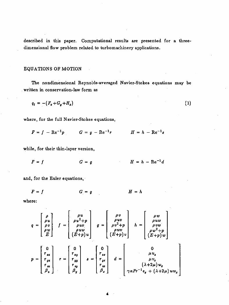
The nondimensional Reynolds-averaged Navier-Stokes equations may bewritten in conservation-law form as

= -(Fs+G,+Hg) (1)

where, for the full Navier-Stokes equations,

F = f - Re-1p G = g - Re-1r H = h -

while, for their thin-layer version,

F = f H = h -

and, for the Euler equations,

F = / G = g H = h

where:

9 =

P -

PpupvpwE .

0

TyxTa

. P* .

f =

r =

pu '

puvpuw

(E+p}u

0JCW

wr«y

. f t , .

9 =

s =

0 '

TyzTzz

. P > .

pv pwpuv puw

pvz+p h = pvwpwv pw2+p

(E+p)v (E+p)w

d =

0

£"*

(\+2n)wg

1KPr-le, +(X+2n)ww g

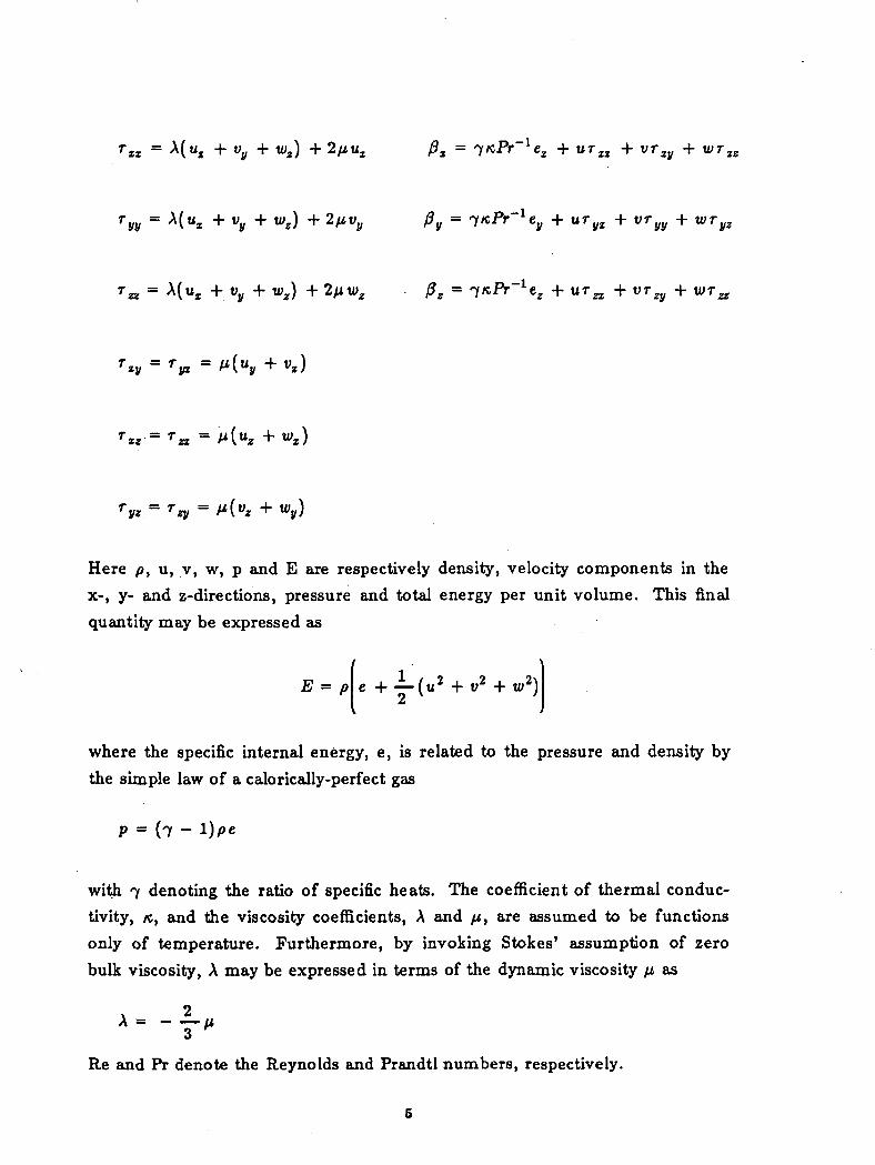
= A(u, + vy + wg) + 2/zuz ft, = 7/cJV lez

ryy = A(u z + vy + wg) + 2ftvy py = ~/KPr ley + ury x + vryy + wryz

vrzy

Here p, u, y, w, p and E are respectively density, velocity components in the

x-, y- and z-directions, pressure and total energy per unit volume. This final

quantity may be expressed as

E = p\t +4-("2 + v* +

where the specific internal energy, e, is related to the pressure and density by

the simple law of a calorically-perfect gas

p = (7 - l)pe

with 7 denoting the ratio of specific heats. The coefficient of thermal conduc-

tivity, /c, and the viscosity coefficients, A and /z, are assumed to be functions

only of temperature. Furthermore, by invoking Stokes' assumption of zero

bulk viscosity, A may be expressed in terms of the dynamic viscosity /z as

Re and Pr denote the Reynolds and Prandtl numbers, respectively.

Although, for simplicity, the equations of motion are presented here writtenin Cartesian coordinates, it is well known that their strong conservation lawform may be maintained under an arbitrary time-dependent transformation ofcoordinates. Explicit detail concerning the generalized-coordinate version ofthese equations, which is employed in the computations to be discussed subse-quently is available in [23].

Note that, in practice, the thin-layer assumption is implemented by using abody-fitted coordinate system and neglecting the viscous terms in the coordi-nate directions along the body. For Cartesian coordinates, with x and yrepresenting the body-conforming coordinates, the thin-layer version of theNavier-Stokes equations is as given above.

The effects of turbulence are simulated by means of a two-layer algebraiceddy viscosity model. In the stress terms of the Navier-Stokes equations, thecoefficient of dynamic viscosity, //, is replaced by //+/*,, where p, is thecoefficient of eddy viscosity. Similarly, in the heat flux terms, the coefficientof thermal conductivity, /c, is replaced by /c+ c //,/Pr,, where Pr, is the tur-p t t \ibulent Prandtl number. The eddy viscosity is determined by the method of

Baldwin and Lomax [24].

SOLUTION METHODOLOGY

In order to minimize the cost of simulating complex, three-dimensionalviscous flow over complete configurations, the following strategy has beendeveloped:

a. Use a robust and flexible explicit flow solver capable of simulating eithersteady or unsteady flow with the Euler, thin-layer Navier-Stokes or fullNavier-Stokes equations.

b. Distribute grid points optimally by making use of locally-embedded gridrefinements.

c. Make use of a flow simulation hierarchy ranging from the Euler equations

6

through the full Navier-Stokes equations in order to minimize the computa-

tional work per grid point.

d. Accelerate the convergence of steady flow simulations by means of an expli-

cit multiple-grid technique which may be applied, without modification, to

the entire hierarchy of model equations.

e. Take advantage of the explicit nature of the algorithm by mapping it onto a

supercomputer architecture consisting of multiple vector-processing CPU's

and thus enhance its performance by means of both vectorization and mul-

titasking.

Further detail concerning this strategy is provided below.

Basic Flow Solver

The integration scheme used here is the two-step Lax-Wendroff method

due to MacCormack [25]. The forward predictor - backward corrector version

of this method may be written as

At („„ „„ \~ ~A7l '';''*+1 ~ '•'•*/

At2Ay

At2Az

where:

First derivatives in the viscous terms are backward differenced in the predictor

and forward differenced in the corrector.

This version of MacCormack's scheme is used here for convenience. Any

of its many variants could also be used, as could any other one- or two-step

Lax-Wendroff scheme [26]. In fact, the class of fine-grid methods with which

the convergence acceleration technique described below may be applied appears

to be quite large, including schemes not of Lax-Wendroff type [27].

The advantages of MacCormack's method, in the present context, are its

explicit nature, simplicity and low operations count. A disadvantage is its con-

ditional stability and the severe time-step size limitation which this imposes for

viscous flows, in particular. The ill effects of conditional stability are mitigated

through the use of embedded grid refinements and convergence acceleration.

Embedded Meshes

The embedded-mesh technique developed for the present application is a

generalization of that employed in [19] to obtain two-dimensional Euler solu-

tions. The computational domain is divided into regions requiring grids of

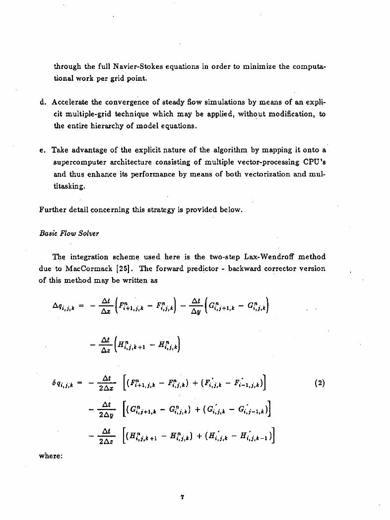
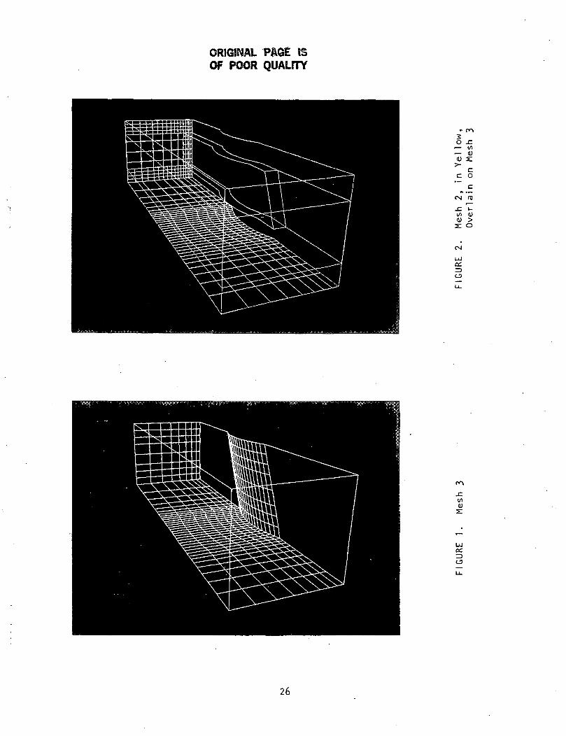
differing fineness and the resolution of different flow physics. At present, forsimplicity, this partitioning is done a-priori. However, solution-adaptive grid-ding based on this technique is possible. Figures 1 through 5 show typical loca-

tions for the mesh regions employed in the computations described subse-

quently in this paper. Note that, where mesh lines are illustrated, their spacing

is much coarser than that employed in the computations. This has been done

for clarity of illustration. Figure 1 shows mesh 3, in white. This mesh covers

the entire computational domain. Figure 2 overlays, in yellow, the regions col-lectively referred to as mesh 2. Figure 3 shows, in cyan, the mesh-1 regions

projected onto mesh 3. In Figure 4, meshes 1 through 3 are assembled into a

single illustration. Figure 5 simply adds wing surface grid lines to this assem-

blage. The mesh-1 regions contain the finest grids. Mesh-2 regions are coarserby a factor of 2 in each dimension. Mesh 3 is coarser again by a factor of 2 in

each dimension. From this example, it is easy to see that quite general collec-

tions of embedded meshes may be constructed in this manner. The embedded

meshes are not disjoint. Rather, given a mesh labelled m, all coarser meshes

from m+ 1 through the coarsest mesh used in the computation underlie it.

This property, together with the coarsening factor of 2, facilitate the use of the

multiple-grid convergence technique described below.

Points on a boundary between two mesh regions belong to the coarser

region. Where mesh regions reach the boundaries of the computational

domain, boundary conditions are applied consistent with the finest mesh reach-

ing the boundary segment in question. The flowfield updating begins with

mesh 1. After one timestep on mesh 1, mesh 2 is updated exterior to mesh 1

while convergence acceleration is applied at the mesh-2 points interior to mesh1. Next, mesh 3 is updated exterior to mesh 2 while convergence acceleration

is applied at the mesh-3 points interior to mesh 2. Updating proceeds in this

fashion until the global mesh has been advanced by one timestep. Then the

updating cycle is completed by applying convergence acceleration to coarsenings

of the global grid. This cycle is repeated until the desired measure of conver-

gence is satisfied.

Simulation Hierarchy

In order to minimize the computational work to obtain a flowfield solution

of specified accuracy and physical resolution, different approximations to the

Navier-Stokes equations are used in different mesh regions. In the example

illustrated in Figures 1 through 5, the full Navier-Stokes equations are solved

on mesh 1, the thin-layer Navier-Stokes equations are solved on mesh 2 and

the Euler equations are solved on mesh 3. In this way the physics contained in

the model equations and the resolving power of the various meshes are

matched to each other.

9

Convergence Acceleration

Given the fine-grid corrections, 5q, we wish to use successively coarser

grids to propagate this information throughout the computational domain, thus

accelerating convergence to the steady state while maintaining the accuracy

determined by the fine-grid discretization. Given a basic fine grid with the

number of points in each direction expressible as n(2*j+ 1 for p and n integers

such that p ^ 0 and n ^ 2, where p is the number of grid coarsenings and n is

the number of coarsest-grid intervals, let successively coarser grids be defined

by successive deletion of every other point in each coordinate direction.

Although it is quite probable that a large variety of coarse-grid accelerationschemes may be constructed, we limit our attention here to those explicit

schemes based on Lax-Wendroff methods. Such an acceleration scheme maybe expressed as

By introducing Eqn.(l), this may be rewritten as

At*^co«r« = -*(P, + Gy + HM) - ^-(Fx + Gy + H,)t

Observing that

A9 --A*(i; +Gy +H,)

we obtain

(J, + Gy + H,)t (3)

Various acceleration schemes may now be derived, according to the .way inwhich the second term on the right-hand side of Eqn.(3) is treated.

10

If we let

-(F, + G y + H t ) t = [A(F t +G,+HJ] , + (B(F, + G, + H,)],

+ ( C ( F t + G y + H z ) ] z

where A, B and C are the Jacobian matrices

A = d F f i q , B = d G f i q a n d C = d H / d q

we obtain the class of Jacobian-based acceleration schemes, of which the

method due to Ni [28] is a member.

If, on the other hand, we let

(F, + Gy + H,}t « ±-[ (F. + G y + F.)"*1 - (F, +G,+H.

where

Fn = F(qn) , Gn = G(g n ) , Hn = H ( q n )

Fn+l = F(qn + Ag) , Gn+l = G(q n + A?) , Hn+l = H(q n + Ag)

we obtain the class of flux-based schemes introduced in [29].

In both classes of schemes, Aq is approximated by a restriction of the fine-

grid value of 6q and second-order accurate spatial differencing is used. For

example, a simple Jacobian-based acceleration scheme may be written as

This scheme is contrasted in Fig. 6 with its one-step Lax-Wendroff analog, writ-

ten on the fine grid. That one-step scheme may be written as

11

*»-f E 2 E '-<-£-"-./=±1 n»=±l n=±l

where Aq is not approximated as a restriction of some £q, as in the coarse-gridscheme, but is rather computed as

A*4Az

Af

4 Ay

~ G i , J ,k

All results reported in this paper use flux-based convergence acceleration.

In the sequential grid updating algorithm, illustrated in Fig. 7a, the solutionis advanced over one multiple-grid cycle as follows. First a fine-grid correction,tfq,, is computed. Then £q, is restricted to the next-coarser grid, where £q« is

12

computed. The £q~ correction is both restricted to grid 3 and prolonged to grid1, where it provides an additional update to the fine-grid solution. On grids 3through N-l the procedure is analogous to that on grid 2. When Sq^ has been

thcomputed and prolonged to grid 1 to provide the N update to the fine-gridsolution, the next multiple-grid cycle is ready to begin.

Observe that when the components of the sequential grid updating algo-rithm (namely, the fine- and coarse-grid schemes) are both explicit, it is partic-

ularly easy to vectorize. However, the effectiveness of vectorizing the coarse-

grid scheme is limited by the progressively shorter vectors which may be con-structed on the successively coarser grids. Such an explicit sequential algorithmmay also be run on a Multiple Instruction-Multiple Data (MIMD) machine bysplitting each grid, in turn, across the total number of processors available. An

implicit sequential grid updating algorithm would probably not vectorize as welland also require additional redesign to run on a parallel processor.

The parallel coarse-grid algorithm, illustrated in Fig. 7b, removes thedependence of grids 3 through N upon their immediate predecessors. In partic-ular, <5q, is now restricted to each of grids 2 through N. All of these coarsegrids may then be updated simultaneously and independently of each other.This allows the mesh points on grids 2 through N to be assembled into onevector in order to improve performance on a Single Instruction-Multiple Data

(SIMD) computer. Alternatively, the coarse grids could each be updatedsimultaneously on separate processors of an MIMD machine. This would beattractive, for example, if the coarse-grid scheme were implicit.

A further possibility is the fully parallel algorithm, illustrated in Fig. 7c.Here £q, from the previous cycle is restricted to each of the coarse grids. Thismakes all of the grids 1 through N independent of each other and allows their

simultaneous update.

Observe that dissipative effects have a local character and their influence

need not be taken into account in the construction of acceleration schemes.

Rather, it is the convective terms, with their global character, which are the keyelement in coarse-grid propagation. Hence, acceleration schemes for viscous

is

flow computations may be formulated on the basis of the inviscid equations of

motion. Such a scheme leads to a convergence acceleration procedure which is

independent of the nature of the dissipative terms retained in the viscous

model equations. That is to say: a scheme based on the Euler equations may

be employed, without modification, to accelerate the convergence of viscous

flow computations based on the Navier-Stokes equations, the thin-layer equa-

tions, or any other viscous model equations which contain the full inviscid

Euler equations.

Boundary conditions are not updated during convergence acceleration. This

has the advantage of decoupling the acceleration scheme from both the physical

and numerical nature of these boundary conditions. That is to say: theacceleration scheme always sees a Dirichlet problem. Any numerical damping

terms which may be necessary are also omitted during convergence accelera-

tion. This enhances the modularity of the acceleration scheme.

For all of the results to be discussed subsequently, linear interpolation hasbeen used as the prolongation operator. For the sequential grid updating algo-

rithm, injection is used as the restriction operator. The parallel coarse-grid

algorithm introduces averaging into the restriction operator for grids 3 through

N. The fully parallel algorithm further employs underretaxation of the fine-grid

information restricted from the previous cycle.

Finally, note that, while in this paper multiple-grid convergence acceleration

is applied only to steady flow simulations, it appears that the technique may

extend to the time-accurate computation of some unsteady flows [30, 31].

Multitasking

When attempting to multitask an algorithm for execution on an MIMDmachine, we are concerned with multitasking overhead and algorithm granular-ity. By granularity we mean the time required to execute a multitaskable seg-

ment of the algorithm on a single processor [32]. For a given multitasking

overhead, the best speedup is obtained when algorithm granularity is maximal.Large granularity is usually introduced by top-down programming which

14

exploits global parallelism in the algorithm. Bottom-up programming, on theother hand, exploits algorithm parallelism at a low level by making many parti-tion ings, each on small code segments, such as DO loops containing indepen-

dent statements [33].

The sequential multigrid algorithm contains many opportunities for creating

small granularity parallelism but relatively few opportunities for the sort of

large granularity necessary to produce good multitasking speedup in the face of

non-trivial multitasking overhead. This observation, together with the desira-

bility of non-sequential multigrid schemes for reasons of algorithm flexibility,

led to the construction of the parallel multigrid algorithms described above. Inthese algorithms, grids which are independent of one another may be updatedsimultaneously on separate processors. In fact, such a simple strategy mayresult in a poor load balance across processors because of the differing amounts

of work inherent in updating grids of different coarseness. However, morerefined strategies are possible. Grids may, for example, be grouped togetherinto tasks of approximately equal work, or they may be melded into tasks withother large-grained multitaskable code segments in order to equilibrate proces-sor loading. Notice further that, by multitasking large-grained structures, thevectorization potential of code within these structures remains intact.

NUMERICAL SIMULATION

At present, all of the elements discussed in the section on solution metho-

dology have been encoded and computationally verified in either two or threedimensions, or both. These elements are now being assembled into acomprehensive three-dimensional algorithm. Performance evaluation of thisalgorithm will be completed in March 1986 and reported in the final version of

this paper. For this abstract, although the three-dimensional model problemdesigned to exercise all aspects of the completed algorithm is described, onlyinterim results are discussed. The expected variance between interim and finalresults is indicated, where possible.

15

Physical Problem

As the algorithm described in this paper is designed to efficiently simulate

complex flows over complete configurations, it should be tested under condi-

tions which fully exercise its capabilities. On the other hand, excessive com-

plexity would serve no useful purpose in the initial testing phases of the algo-

rithm. With these considerations in mind, three-dimensional computations are

being carried out for the geometry illustrated in Fig. 8, a rectilinear cascade of

finite-span, swept blades mounted between ehdwalls. The sweep angle ranges

from 0 to 26 degrees. The blade thickness to chord ratio ranges from 0.0 to

0.2. The subcritical computations are performed at an isentropic inlet Mach

number of 0.5. The Mach number for the supercritical computations is 0.675.In the viscous cases, the Reynolds numbers, based on cascade gap and critical

3 5speed, span the approximate range from 8.4 x 10 to 2.0 x 10 .

At the upstream domain boundary, total pressure, total temperature and

flow angle are specified. At the downstream boundary, the static pressure is

fixed. Along inviscid lateral boundaries, the tangency condition is applied,

while, along solid walls, the no-slip condition is applied and the temperature

specified. Symmetry and periodicity are invoked to limit the size of the compu-

tational domain. Uniform flow at the isentropic inlet Mach number is used as

an initial state.

Algorithm Implementation

The mesh structure on which the computations are performed is illustrated

in Figs. 1 through 5. The full Navier-Stokes equations are solved on mesh 1.

The thin-layer Navier-Stokes equations are solved on mesh 2. The Euler equa-

tions are solved on mesh 3. Only steady flows are computed and convergenceacceleration, as described previously, is applied. The entire algorithm is vector-

ized and multitasked to run on a four-processor Cray X-MP or Cray 2.

Computational Results

Sample flowfield results obtained using the basic flow solver with

16

convergence acceleration but without embedded mesh refinements are shownin Figs. 9 through 12. The use of embedded meshes causes no deterioration ofthese results, assuming that the meshes are positioned properly. The final ver-

sion of this paper will contain much more elaborate flowfield results, includingdepiction of corner vortices.

Comparison of the embedded-mesh algorithm with a single-mesh algorithmyields the following general result: the accuracy of the embedded-mesh resultsis essentially that of a global finest mesh, while the convergence rate is like thatof a global coarsest mesh. This observation is consistent with [19]. Thus far,in two-dimensional computations using the Euler and thin-layer Navier-Stokes

equations and three mesh regions, embedding speedups as high as 30 in com-

parison to a single-mesh algorithm have been obtained. Some interim two-dimensional embedding speedups are reported in Table I. Three-dimensional

embeddings using Euler, thin-layer and full Navier-Stokes regions should pro-duce substantially larger speedups.

Multiple-grid convergence acceleration applied to three-dimensional cases,in the absence of mesh embedding, has yielded speedups ranging from 2.5 to

4.7 (see Table II). It is expected that there will be some tradeoff betweenembedding speedup and multigrid speedup in the complete algorithm.

Vectorization of the three-dimensional algorithm without embedded meshesresults in speedups ranging from 3.6 to 5.7 (see Table III). This range shouldremain about the same in the final algorithm.

Using a top-down multitasking approach, the parallel coarse-grid algorithmhas been implemented on a four processor Cray X-MP, for two-dimensionalcases without mesh embedding. Initially, only the coarse grids were multi-tasked so that the performance of parallel grids on a multiprocessor could beevaluated. Then the fine-grid computations were partitioned and multitasked,

and the resultant code was integrated with the parallelized coarse grids. Loadbalancing of the entire scheme completed the study of performance resulting

from the top-down approach.

17

Multitasking results are shown in Table IV. The performance measures arebased on a comparison of xnultitasked code segments with their unitasked ana-logs. The parallel coarse-grid scheme results contained in Table IVa wereobtained with a five-grid multigrid sequence length. Observe that an efficiencyof nearly 90% has been obtained using two processors, but that efficiencydeteriorates to 77% when four processors are used. This deterioration is aresult of distributing multigrid structures containing unequal amounts of workacross four processors, which creates a less than ideal load balance. Table IVb

shows results obtained from multitasking the fine-grid scheme. The fine-gridtasks are fairly evenly balanced, and this code segment performs well on bothtwo and four processors. Processor utilization of 90% or better is achieved.When the four-processor case is recomputed using the low-overhead version ofmultitasking known as microtasking [34], efficiency is improved to 95%. Thefully multitasked multigrid algorithm performance is shown in Table IVc. Ontwo processors, 94% efficiency is obtained, while on four processors, withspeedup by a factor of 3.3 over the unitasked code, efficiency is 83%. Multi-tasking speedups are expected to improve for the complete three-dimensionalcode.

Given that the speedups from the various categories described above aregenerally multiplicative in effect, it is to be conservatively estimated that thecompleted algorithm to be reported in the final version of this paper will pro-duce overall speedups ranging as high as 100.

CONCLUSIONS

An efficient algorithm designed to be used for Navier-Stokes simulations of

complex flows over complete configurations has been presented.

The algorithm makes use of several elements:

A robust explicit basic flow solver

Locally-embedded mesh refinements

A flow simulation hierarchy ranging from the Eulerequations through the full Navier-Stokes equations

18

An explicit multiple-grid convergence accelerationtechnique

Both vectorization and multitasking for efficientexecution on parallel-processing supercomputers

Results are presented for a problem representative of turbomachinery appli-cations. These results validate the algorithm and provide grounds for optimism

regarding its future application to more challenging internal and external flows.

Based on the interim performance data available at this writing, it is

estimated that the completed algorithm to be reported in the final version of

this paper will produce overall speedups ranging as high as 100.

ACKNOWLEDGEMENTS

The research reported here is funded in part by the NASA Ames Research

Center (Grant No. NCC-2-344) and the Air Force Office of Scientific Research

(Grant No. AFOSR-85-289). Some of the computing time has been contri-

buted by Cray Research, Inc. All of this support is gratefully acknowledged.

19

REFERENCES

1. Rubbert, P.E.: The Emergence of Advanced Computational Methods in theAerodynamic Design of Commercial Transport Aircraft. Proceedings of theInternational Symposium on Computational Fluid Dynamics, Sponsored bythe Japan Society of Computational Fluid Dynamics, Tokyo, 1985.

2. Shang, J.S. and Scherr, S.J.: Navier-Stokes Solution of the Flow FieldAround a Complete Aircraft. AIAA Paper 85-1509, 1985.

3. Bailey, F.R.: Overview of NASA's Numerical Aerodynamic Simulation Pro-gram. Proceedings of the International Symposium on Computational FluidDynamics, Sponsored by the Japan Society of Computational Fluid Dynam-ics, Tokyo, 1985.

4. Peterson, V.L.: Impact of Computers on Aerodnamics Research andDevelopment. Proceedings of the IEEE, Vol. 72, No. 1, January 1984.

5. Aki, T. and Yamada, S.: A Supercomputer Simulation of Three Dimen-sional Viscous Flow. Proceedings of the International Symposium on Com-putational Fluid.Dynamics, Sponsored by the Japan Society of Computa-tional Fluid Dynamics, Tokyo, 1985.

6. Deiwert, G.S., Rothmund, H.J. and Nakahashi, K.: Simulation of ComplexThree-Dimensional Flows. Proceedings of the International Symposium onComputational Fluid Dynamics, Sponsored by the Japan Society of Compu-tational Fluid Dynamics, Tokyo, 1985.

7. Flores, J.: Convergence Acceleration for a Three-Dimensional EulerNavier-Stokes Zonal Approach. AIAA Paper 85-1495, 1985.

8. Fujii, K. and Obayashi, S.: The Development of Efficient Navier-StokesCodes for Transonic Flow Field Simulations. Proceedings of the Interna-tional Symposium on Computational Fluid Dynamics, Sponsored by theJapan Society of Computational Fluid Dynamics, Tokyo, 1985.

9. Hoist, T.L., Gundy, K.L., Flores, J., Chaderjian, N.M., Kaynak, U. andThomas, S.D.: Numerical Solution of Transonic Wing Flows Using anEuler/Navier-Stokes Zonal Approach. AIAA Paper 85-1640, 1985.

10. Hung, C.M.: Computation of Three-Dimensional Shock Wave andBoundary-Layer Interactions. Proceedings of the International Symposiumon Computational Fluid Dynamics, Sponsored by the Japan Society ofComputational Fluid Dynamics, Tokyo, 1985.

20

11. Kordulla, W.: The Computation of Three-Dimensional Transonic ViscousFlows with Separation. Proceedings of the Ninth International Conferenceon Numerical Methods in Fluid Dynamics, Lecture Notes in Physics, Vol.218, Springer, 1985.

12. Li, C.P.: Numerical Procedure for Three-Dimensional Hypersonic ViscousFlow over Aerobrake Configuration. Proceedings of the International Sym-posium on Computational Fluid Dynamics, Sponsored by the Japan Societyof Computational Fluid Dynamics, Tokyo, 1985.

13. Johnson, G.M. and Swisshelm, J.M.: Multiple-Grid Solution of the Three-Dimensional Euler and Navier-Stokes Equations. Proceedings of the NinthInternational Conference on Numerical Methods in Fluid Dynamics, Lec-ture Notes in Physics, Vol. 218, Springer, 1985.

14. Mik atari an, R.R., Rapagnani, N.L. and Hendricks, W.L.: RAVEN: A Com-puter Model for the Solution of the Time-Dependent, Three DimensionalNavier-Stokes Equations with Nonequilibrium Chemistry. Proceedings ofthe International Symposium on Computational Fluid Dynamics, Sponsoredby the Japan Society of Computational Fluid Dynamics, Tokyo, 1985.

15. Roger, R.P., Thoenes, J. and Robertson, S.J.: Viscous Flow Computationsfor a Two-Duct Version of the Space Shuttle Main Engine Hot Gas Mani-fold. Proceedings of the International Symposium on Computational FluidDynamics, Sponsored by the Japan Society of Computational Fluid Dynam-ics, Tokyo,1985.

16. Koeck, C. and Chattot, J.J.: Computation of Three-Dimensional VortexFlows Past Wings Using the Euler Equations and a Multiple-Grid Scheme.Proceedings of the Ninth International Conference on Numerical Methodsin Fluid Dynamics, Lecture Notes in Physics, Vol. 218, Springer, 1985.

17. Rizzi, A. and Purcell, C;J.: Cyber 205 Exploration of Inviscid Vortex-Stretched Turbulent Shear-Layer Flow. Proceedings of the InternationalSymposium on Computational Fluid Dynamics, Sponsored by the JapanSociety of Computational Fluid Dynamics, Tokyo, 1985.

18. Benek, J.A., Buning, P.G. and Steger, J.L.: A 3-D Chimera Grid Embed-ding Technique. AIAA Paper 85-1523, 1985.

19. Usab, W.J.: Embedded Mesh Solutions of the Euler Equation Using aMultiple-Grid Method. Doctoral Dissertation, Department of Aeronauticsand Astronautics, Massachusetts Institute of Technology, 1983.

21

20. Eberhardt, S. and Baganoff, D.: Overset Grids in Compressible Flow.AIAA Paper 85-1524, 1985.

21. Johnson, G.M., Swisshelm, J.M. and Kumar, S.P.: Concurrent-ProcessingAdaptations of a Multiple-Grid Algorithm. AIAA Paper 85-1508, 1985.

22. Stevens, K.G., Jr.: Efficiency of CFD Algorithms on Multiprocessor Archi-tectures. Proceedings of the International Symposium on ComputationalFluid Dynamics, Sponsored by the Japan Society of Computational FluidDynamics, Tokyo, 1985.

23. Pulliam, T.H. and Steger, J.L.: Implicit Finite-Difference Simulation ofThree-Dimensional Compressible Flow. AIAA J., Vol. 18, No. 2, pp. 159-167, 1980.

24. Baldwin, B.S. and Lomax, H.: Thin-Layer Approximation and AlgebraicModel for Separated Turbulent Flows. AIAA Paper 78-257, 1978.

25. MacCormack, R.W.: The Effect of Viscosity in Hypervelocity ImpactCratering. AIAA Paper 69-354, 1969.

26. Johnson, G.M.: Multiple-Grid Acceleration of Lax-Wendroff Algorithms.NASA TM-82843, 1982.

27. Stubbs, R.M.: Multiple-Gridding of the Euler Equations with an ImplicitScheme. AIAA Paper 83-1945, 1983.

28. Ni, R.H.: A Multiple Grid Scheme for Solving the Euler Equations.AIAA Paper 81-1025, 1981.

29. Johnson, G.M.: Flux-Based Acceleration of the Euler Equations. NASATM-83453, 1983.

30. Stubbs, R.M.: Private Communication, 1983.

31. Jespersen, D.C.: A Time-Accurate Multiple-Grid Algorithm. AIAAPaper 85-1493, 1985.

32. Larson, J.L.: Practical Concerns in Multitasking on the Cray X-MP.Workshop on Using Multiprocessors in Meteorological Models, ECMLOF,Reading, England, 3-6 December 1984.

33. Larson, J.L.: Multitasking on the Cray X-MP-2 Multiprocessor. Computer,pp. 62-69, 1984.

22

34. Booth, M.: Microtasking - A Brief Design Summary. Cray Research, Inc.Internal Memorandum, 1985.

23

TABLES

Table I. Interim Two-Dimensional Embedding Speedups

Inviscid Subcritical 16.4Inviscid Supercritical 6.1Turbulent Viscous 30.2

Table II, Interim Three-Dimensional Multigrid Speedups

Inviscid Subcritical 4.7Inviscid Supercritical 2.5Turbulent Viscous 4.4

Table III. Interim Three-Dimensional Vectorization Speedups

Automatic ExplicitScalar Vectorization Vectorization

Inviscid Subcritical 1.0 4.2 5.7Inviscid Supercritical 1.0 3.1 4.9Turbulent Viscous 1.0 2.6 3.6

24

Table IVa. Interim Two-Dimensional Multitasked Coarse-Grid Performance

Machine

Cray X-MP

2 Processors

Speedup

1.78

Efficiency

0.89

4 Processors

Speedup

3.06

Efficiency

0.77

Table IVb. Interim Two-Dimensional Multitasked Fine-Grid Performance

Machine

Cray X-MPCray X-MPwithmicro task ing

2 Processors

Speedup

1.91

1.93

Efficiency

0.96

0.97

4 Processors

Speedup

3.58

3.78

Efficiency

0.90

0.95

Table IVc. Interim Two-Dimensional Multitasked Complete Scheme Performance

Machine

Cray X-MP

2 Processors

Speedup

1.87

Efficiency

0.94

4 Processors

Speedup

3.30

Efficiency

0.83

25

ORIGINAL PAGE ISOF POOR QUALfTY

I— t/1— 0)

cc o

c

CM OJ

IS> <U

a:rjCD

.Cui0)

a:

26

ORIGINAL PAGE !SOF POOR QUALITY

013O

-C4-1

ISI<u-C01a)

-3-

LUOL

C ui(0 0)>- 2:

(_)C

C O

T- ID

1/1 <ua) >2: o

LU(£.

27

fSOF POOR QUALITY

r<-\<U

. c u e01 ro 33 u- OO i- -ci- n co.c to4J l/l

cn d)«— c c

ui S —I(!)

JZ -C -O{ft -M • —0) — u

UA

LUo:

CJ3

28

CMI

01

<uu

I0)I/)L.IDoo

<uQJ£uto

I0)ini_mo

•oc

<uc

•— i_

a)c

O

IU

0)

uto

•oca>ixID

a.0)

COI

co

o

1-(0a

so

LUQC3U

29

R - Restriction of 6q as Coarse-Grid Aq

P - Prolongation of <5q to Fine Grid

N

t+At

a. Sequential Algorithm

N

t+At

t-At

t+Atb. Parallel Coarse Grids c. Fully Parallel Scheme

FIGURE 7. Multiple-Grid Algorithm Information Flow

30

0)>

o<uo.I/)1_<U

Q-

(U

<U•OTOO(/)(0

coI/)c(1)

<u0)

OJIoTOCo

3Q.

OO

ooUJoe

co

o<uto

31

seg

o 9

Uu(CL_orin

o.

.H O- O O Q DOOOG

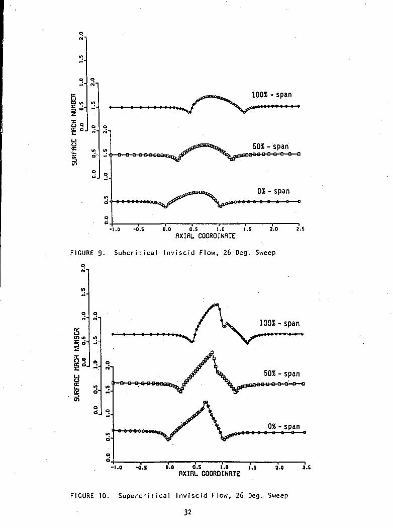
O'O O OOfrtH

100% - span

50%-'spanJOOQ a Q o o o

0% - spanoooo o o o o o o o

-1.0 -0.5 0.0 O.S 1.0 I.S 2.0 2.5flXIflL COOROlNflTE

FIGURE 3. Subcr i t ical Inv isc id Flow, 26 Deg. Sweep

100% - span> « » • • « > • • i

-1.0 -O.S 0.0 O.S 1.0 I.S 2.0 2.SRXIfiL COOROlNflTE

FIGURE 10. Supercrit ical Inviscid Flow, 26 Deg. Sweep

32

g

OM 6'0 8'0 ro 9'0 S'O V'O E'O Z'O I'D O'O30NU1SIQ 3SH3ASNyHi

-fl-ea

<UQC

co

c(0Q.

OLA

Q.0>

cn0)

voCM

CJ

uoLJ

i

autM

a:

o

a)oc

C(Da.to

OLA

- Q.3 <uO 0)

U. CO

OJ O)C 0)

— QE(D vD-I CM

ce.=jC3

o'i 6'o e'o ^'o 9*0 s'o vo c'o z'o ro 0*030NU1SIQ

33