COLOR CODING FOR A FACSIMILE SYSTEM

by

ROBERT DAVID SOLOMON

B.S.E.E., Polytechnic Institute of Brooklyn

(1967)

S.M., Massachusetts Institute of Technology

(1968)

E.E., Massachusetts Institute of Technology

(1970)

SUBMITTED IN PARTIAL FULFILLMENT OF THE

REQUIREMENTS FOR THE DEGREE OF

DOCTOR OF PHILOSOPHY

at the

MASSACHUSETTS INSTITUTE OF TECHNOLOGY

August 1975

1~~

Signature of Author. . . . . . . . . . . . . .

Department of Elect,ical Engineering, August 29, 1975

Certified by .0.......... .. . . . . .

T is Supervisor

Accepted by. . . c. . .Chairman, Departmental Committee on Graduate Students

Erchives

OCT 271975allRAR1oS

- 2 -

COLOR CODING FOR A FACSIMILE SYSTEM

by

Robert David Solomon

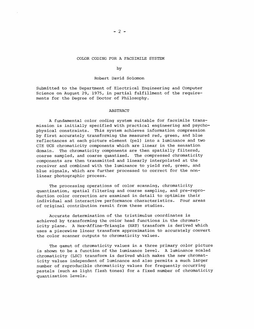
Submitted to the Department of Electrical Engineering and Computer

Science on August 29, 1975, in partial fulfillment of the require-

ments for the Degree of Doctor of Philosophy.

ABSTRACT

A fundamental color coding system suitable for facsimile trans-

mission is initially specified with practical engineering and psycho-

physical constraints. This system achieves information compression

by first accurately transforming the measured red, green, and blue

reflectances at each picture element (pel) into a luminance and two

CIE UCS chromaticity components which are linear in the sensation

domain. The chromaticity components are then spatially filtered,

coarse sampled, and coarse quantized. The compressed chromaticity

components are then transmitted and linearly interpolated at the

receiver and combined with the luminance to yield red, green, and

blue signals, which are further processed to correct for the non-

linear photographic process.

The processing operations of color scanning, chromaticity

quantization, spatial filtering and coarse sampling, and pre-repro-

duction color correction are examined in detail to optimize their

individual and interactive performance characteristics. Four areas

of original contribution result from these studies.

Accurate determination of the tristimulus coordinates is

achieved by transforming the color head functions in the chromat-

icity plane. A Hex-Affine-Triangle (HAT) transform is derived which

uses a piecewise linear transform approximation to accurately convert

the color scanner outputs to chromaticity values.

The gamut of chromaticity values in a three primary color picture

is shown to be a function of the luminance level. A luminance scaled

chromaticity (LSC) transform is derived which makes the new chromat-

icity values independent of luminance and also permits a much larger

number of reproducible chromaticity values for frequently occurring

pastels (such as light flesh tones) for a fixed number of chromaticity

quantization levels.

-53-

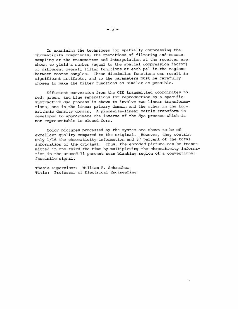
In examining the techniques for spatially compressing the

chromaticity components, the operations of filtering and coarse

sampling at the transmitter and interpolation at the receiver are

shown to yield a number (equal to the spatial compression factor)

of different overall filter functions at each pel in the regions

between coarse samples. These dissimilar functions can result in

significant artifacts, and so the parameters must be carefully

chosen to make the filter functions as similar as possible.

Efficient conversion from the CIE transmitted coordinates to

red, green, and blue separations for reproduction by a specific

subtractive dye process is shown to involve two linear transforma-

tions, one in the linear primary domain and the other in the log-

arithmic density domain. A piecewise-linear matrix transform is

developed to approximate the inverse of the dye process which is

not representable in closed form.

Color pictures processed by the system are shown to be of

excellent quality compared to the original. However, they contain

only 1/16 the chromaticity information and 37 percent of the total

information of the original. Thus, the encoded picture can be trans-

mitted in one-third the time by multiplexing the chromaticity informa-

tion in the unused 11 percent scan blanking region of a conventional

facsimile signal.

Thesis Supervisor: William F. Schreiber

Title: Professor of Electrical Engineering

- 4-

Acknowledgments

Due to outside professional commitments, the rate of progress of

this thesis has varied considerably over the past four years. During

this time Professor Schreiber, my thesis and graduate advisor, has been

very understanding and has given me realistic encouragement and support

at various critical phases. My choice of readers, Doctors Richards,

Tribus, and Troxel , has proven very fortuitous since the readers rep-

resented diverse areas of specialization, professional backgrounds, and

philosophical outlooks which they enthusiastically applied to provide

a broader insight into my multidisciplinary thesis problem. The late

Professor Mason was an original reader and I am greatly indebted to him

for his personal interest and encouragement in the early stages of my

research.

My thesis research utilized the facilities of the Research Laboratory

of Electronics and I am grateful for the generous support of many competent

staff members. The first four years of my research were supported under

a grant to MIT from the Associated Press. In addition, the General Radio

Company in part supported the early period of my graduate work.

TABLE OF CONTENTS

Page

Abstract - - - - - - - - - - - - - - - - - - - - - - - - - - - - - - - 2

Acknowledgments - - - - - - - - - - - - - - - - - - - - - - - - - - - 4

Table of Contents - - - - - - - - - - - - - - - - - - - - - - - - - - 5

List of Figures - - - - - - - - - - - - - - - - - - - - - - - - - - - 7

Chapter 1. Introduction - - - - - - --- - - - - - - - - - - - - - - 10

1.1 - The Basic Problem - - - - - - - - - - - - - - - - - - - - 11

1.2 - Fundamental Constraints on the Color Facsimile System - - 13

1.3 - A Preliminary Model of the Color Facsimile System - - - - 17

1.4 - Summary - - - - - - - - - - - - - - - - - - - - - - - - - 19

Chapter 2. Color Space and Chrominance Quantization - - - - - - - - 21

2.1 - Colorimetry - - - - - - - - - - - - - - - - - - - - - - - 22

2.2 - Color Space Representations and Transformations ----- 26

2.3 - Uniform Sensation Color Space - - - - - - - - - - - - - - 30

2.4 - The Luminance Scaled Chromaticity (LSC) Transform - - - - 35

Chapter 3. The Chrominance Spatial Filtering Process - - - - - - - - 49

3.1 - The Pschophysical Basis For Chrominance Spatial Filtering 50

3.2 - The Overall Filter Function - - - - - - - - - - - - - - - 52

3.3 - Luminance Filtering For the LSC Transform - - - - - - - - 67

Chapter 4. Colorimetric Measurement and Photographic Reproduction

Approximations - - - - - - - - - - - - - - - - - - - - - 70

4.1 - The Color Photographic Process - - - - - - - - - - - - - - 71

4.2 - Quasi-Tristimulus Color Measurement - - - - - - - - - - - 76

4.3 - Colorimetrically Accurate Photographic Reproduction - - - 90

- 6 -

Chapter 5.

5.1 -

5.2 -

5.3 -

5.4 -

Chapter 6.

6.1 -

6.2 -

6.3 -

Appendix I.

Appendix II

Appendix I

Appendix I

Appendix V

Appendix V

RD -f "n es

Page

Simulation of the Color Facsimile System - - - - - - - - 101

Introduction - - - - - - - - - - - - - - - - - - - - - - 102

The Color Scanner - - - - - - - - - - - - - - - - - - - - 104

The Computer and Software Systems - - - - - - - - - - - - 108

Reconstruction of Color Pictures - - - - - - - - - - - - 112

Color Picture Evaluation and Conclusions - - - - - - - - 114

Subjective Analysis of Compressed Color Pictures - - - - 115

Topics For Further Research - - - - - - - - - - - - - - - 120

Conclusions - - - - - - - - - - - - - - - - - - - - - - - 122

Linear Transformation To A New Set of Color Primaries - 123

Inversion of Bilinear Chromaticity Color Space - - - - 125

[I. Derivation of the LSC Transform - - - - - - - - - - - 126

7. A Mathematical Analysis of Dye Correction - - - - - - - 129

. Color Transform For New Primaries With Specified

Chromaticities - - - - - - - - - - - - - - - - - - - - 134

[. Numeric System Parameters and Transforms - - - - - - - 136

- - - - - - - - - - - - - - - - - - - - - - - - - - - - - 140

Biographical Note - - - - - - - - - - - - - - - - - - - - - - - - - 143

- 7 -

LIST OF FIGURES

Figure Page

1-1 Basic Model of a Color Facsimile System - - - - - - - - - 18

2-1 CIE R,G,B Matching Functions - - - - - - - - - - - - - -- 23

2-2 Luminous Efficiency Function - - - - - - - - - - - - - - 25

2-3 R,G,B Primary Color Space - - - - - - - - - - - - - - - - 27

2-4 Linearly Transformed L, C1 , C2 Color Space - - - - - - - 29

2-5 UCS Chromaticity Diagram - - - - - - - - - - - - - - - - 33

2-6 Bilinearly Transformed C1, C2 Color Space - - - - - - - - 34

2-7 R,G,B Separations of Group Picture - - - - - - - - - - - 36

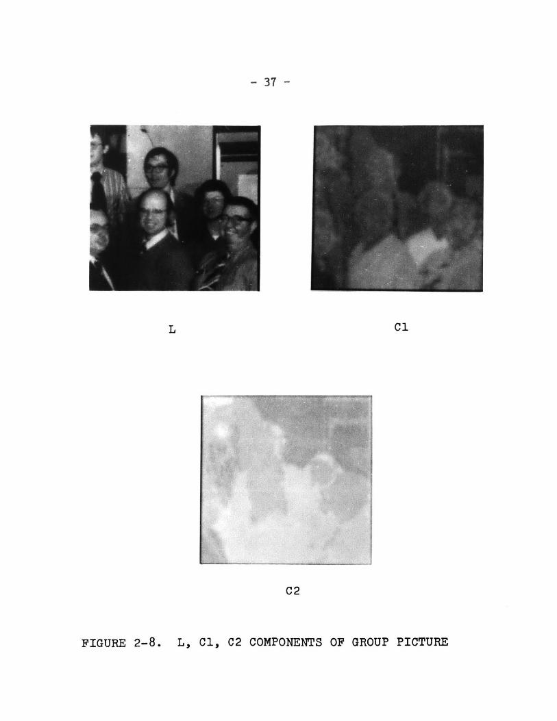
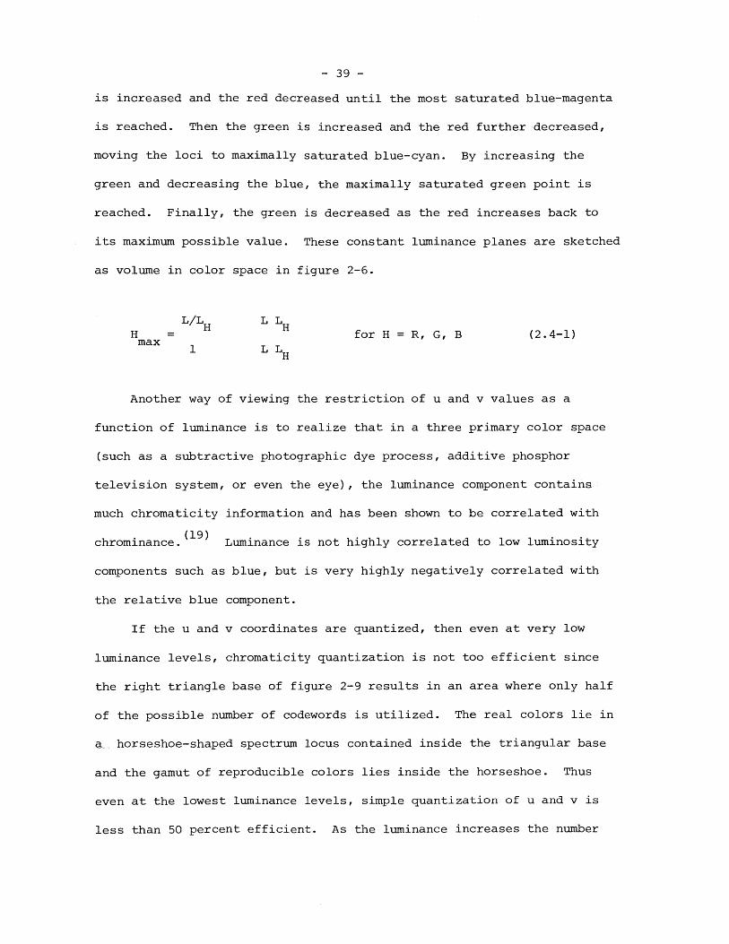
2-8 L, C1, C2 Components of Group Picture - - - - - - - - - - 37

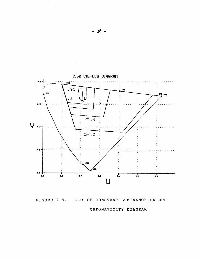
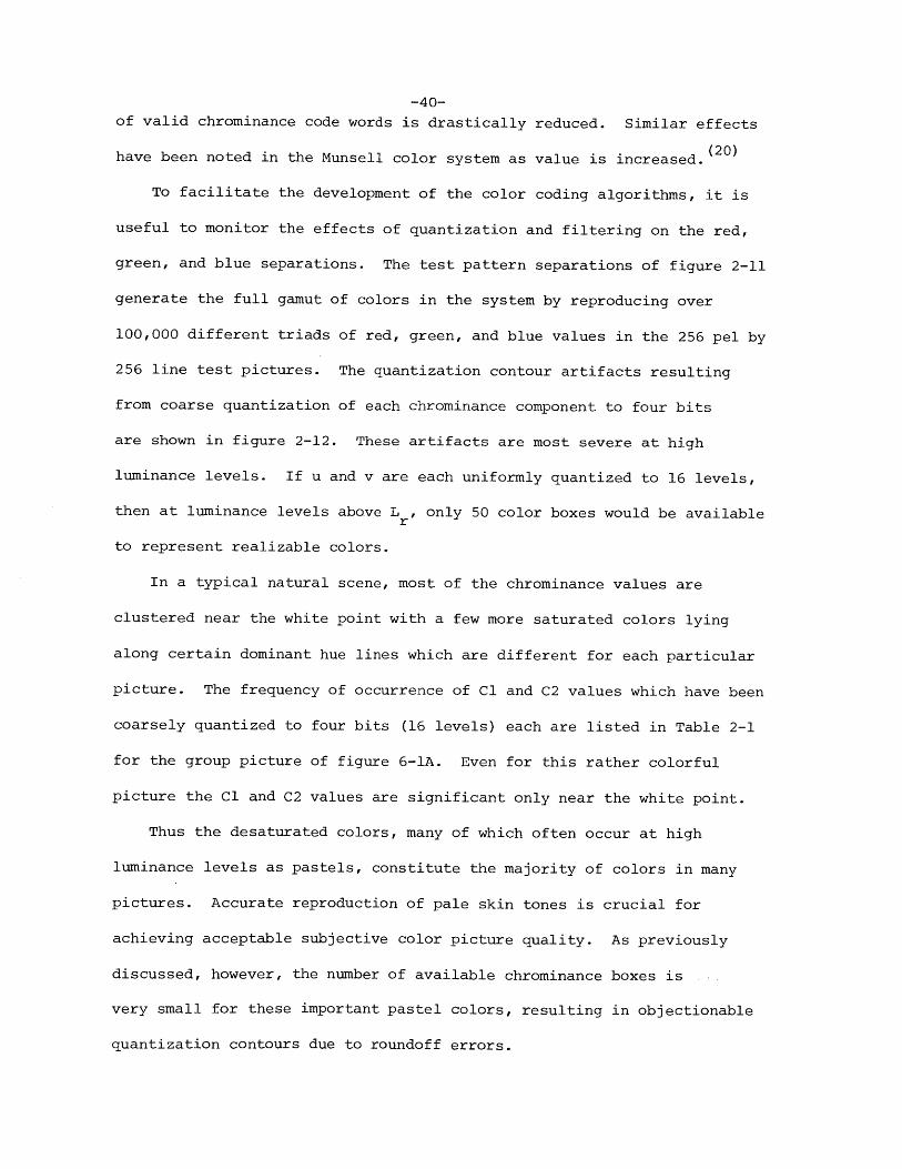
2-9 Chromaticity Loci at Constant Luminance - - - - - - - - - 38

2-10 L and LSC Transformed C1 , C 2 Components of Group Picture- 42

2-11 R,G,B Separations of Test Picture - - - - - - - - - - - - 43

2-12 R,G,B Separations of Compressed Test Picture - - - - - - 44

2-13 R,G,B Separations of LSC Transformed Compressed Test

Picture - - - - - - - - - - - - - - - - - - - - - - - - - 47

3-1 The Four Stages of the Overall Filter Function - - - - - 53

3-2 Two Dimension Filter Block Diagram - - - - - - - - - - - 55

3-3 The Symmetric Transmitter Filter Function - - - - - - - - 57

3-4 Two Dimensional Coarse Sampling and Interpolation - - - - 58

3-5 The Continuous Interpolation Filter Function - - - - - - 59

3-6 The Sampled Interpolation Function - - - - - - - - - - - 59

3-7 Triangular Transmitter Filter Function - - - - - - - - - 62

3-8 OFF for the Transmitter Filter of Figure 3-7 - - - - - - 63

3-9 Modified Transmitter Filter Function - - - - - - - - - - 64

3-10 OFF for the Modified Filter of Figure 3-9 - - - - - - - - 65

3-11 R,G,B Separations of Test Picture Processed by the OFF

of Figure 3-8 - - - - - - - - - - - - - - - - - - - - - - 66

3-12 LSC Transform Processing - - - - - - - - - - - - - - - - 68

- 8 -

Block Dye Approximation - - - - - - - - - - - - - - - -

Basic Model of the Color Photographic Process - -

Taking Sensitivity of Ektachrome Reversal Film -

Dye Transmission Curves for Ektachrome Slides - -

Density - Log Exposure Curves for Ektachrome Film

Color Head Sensor Response Functions - - - - - -

Color Head Filter Quasi Luminosity Function - - -

Dye Gamut for RC Print Paper Dyes - - - - - - - -

Dye Gamut Measured by the Color Head Filters - -

U-V Affine Transform - - - - - - - - - - - - - -

U-V Transform with Second Order u - - - - - - - -

Hex-Affine-Triangular (HAT) Transform - - - - - -

Transmitter Encoder with Color Head Correction

Transforms - - - - - - - - - - - - - - - - - - -

Receiver Decoder with Pre-dye Primary and Density

4-1

4-2

4-3

4-4

4-5

4-6

4-7

4-8

4-9

4-10

4-11

4-12

4-13

4-14

4-15

4-16

4-17

4-18

4-19

5-1

5-2

5-3

5-4

5-5

Figure Page

73

- - - 75

- - - 75

- - - 75

- - - 77

- - - 80

82

- - - 83

84

86

- - - 88

- - - 89

- - - 91

Transforms - - - - - - - - - - - - - - - - - - - - -

Dye Gamut of Photograph Made Directly from CIE R,G,B

Separations - - - - - - - - - - - - - - - - - - - - -

CIE R,G,B and R',G',B' Primary Triangles - - - - - -

Dye Gamut of Photograph with R',G',B' Coordinates - -

Dye Gamut of Photograph with Hex Dye Correction

Transform - - - - - - - - - - - - - - - - - - - - - -

Overall Chromatic Reproduction Accuracy of the

Facsimile System - - - - - - - - - - - - - - - - - -

PDP-9 Color Image Processing Computer System - - - -

Color Facsimile Scanner Optics - - - - - - - - - - -

Schematic Representation of the Color Head Response

Functions - - - - - - - - - - - - - - - - - - - - - -

Monochrome Receiver and Color Transmitter Facsimile

Interface - - - - - - - - - - - - - - - - - - - - - -

COPS System Block Diagram - - - - - - - - - - - - - -

91

- 93

- 95

- 96

- 98

- 100

- 103

- 105

- 106

- 107

- 110

- 9 -

Figure Page

6-1 Group Picture - - - - - - - - - - - - - - - - - - - - - - 117

a) Scanned Color Corrected Unprocessed Original

b) Scanned Unprocessed Original Without Output DyeCorrection

c) Fully Processed, Compressed with LSC Transform

6-2 Cameraman Picture - - - - - - - - - - - - - - - - - - - - 118

a) Scanned Color Corrected Uncompressed Original

b) Compressed Without LSC Transform

c) Compressed with LSC Transform

6-3 Portrait Picture - - - - - - - - - - - - - - - - - - - - 119

a) Scanned Color Corrected Uncompressed Original

b) Compressed Without LSC Transform

c) Compressed with LSC Transform

TABLES

Table Page

2-1 Frequency of Occurrence of C -C2 Values for the Group

Picture - - - - - - - - - - - - - - - - - - - - - - - - 41

2-2 Frequency of Occurrence of LSC Transformed C 1-C2 Valuesfor the Group Picture - - - - - - - - - - - - - - - - - 48

A-1 Quasi-Luminance Function Accuracy - - - - - - - - - - - 137

A-2 Hexagonal Affine Transform for the Color Head Inputs - 138

A-3 Hexagonal Affine Transform for Pre-Dye Correction - - - 139

- 10 -

I. Introduction

1.1: The Basic Problem

1.2: Fundamental Constraints on the Color Facsimile System

1.3: A Preliminary Model of the Color Facsimile System

1.4: Summary

- 11 -

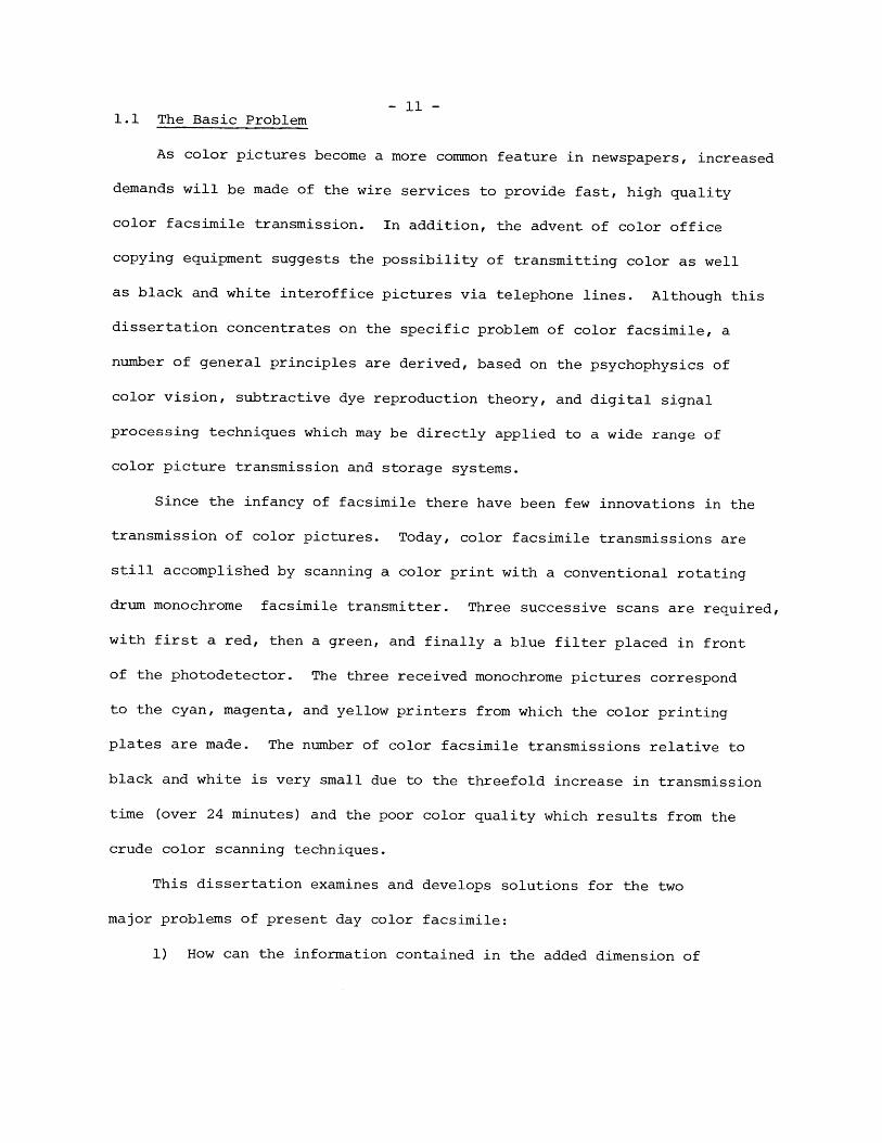
1.1 The Basic Problem

As color pictures become a more common feature in newspapers, increased

demands will be made of the wire services to provide fast, high quality

color facsimile transmission. In addition, the advent of color office

copying equipment suggests the possibility of transmitting color as well

as black and white interoffice pictures via telephone lines. Although this

dissertation concentrates on the specific problem of color facsimile, a

number of general principles are derived, based on the psychophysics of

color vision, subtractive dye reproduction theory, and digital signal

processing techniques which may be directly applied to a wide range of

color picture transmission and storage systems.

Since the infancy of facsimile there have been few innovations in the

transmission of color pictures. Today, color facsimile transmissions are

still accomplished by scanning a color print with a conventional rotating

drum monochrome facsimile transmitter. Three successive scans are required,

with first a red, then a green, and finally a blue filter placed in front

of the photodetector. The three received monochrome pictures correspond

to the cyan, magenta, and yellow printers from which the color printing

plates are made. The number of color facsimile transmissions relative to

black and white is very small due to the threefold increase in transmission

time (over 24 minutes) and the poor color quality which results from the

crude color scanning techniques.

This dissertation examines and develops solutions for the two

major problems of present day color facsimile:

1) How can the information contained in the added dimension of

- 12 -

color (chrominance 1) be compressed and coded to a small fraction

of the black and white luminance information so that a color

picture may be transmitted in the same time as a monochrome

picture (8 minutes) and be subjectively equivalent to the

original?

2) What techniques are necessary to scan an original color print

and make a photographic reproduction from red, green, and blue

separations, so that the color rendition and overall subjective

quality of the output print is acceptably similar to the input

print?

It might be suggested that the second problem has already been solved

since methods for high quality color reproduction using an electronic scanner

are well known and commonly used.(1,2) However, in order to solve the first

problem, the human eye must be somehow fooled into believing that the

compressed picture contains as much information as the original. Colors

should be represented in terms of psychophysical coordinates. These co-

ordinates should also be chosen so that information which is visually

redundant due to the limited color and spatial acuity of the eye can be

easily removed by coarse linear quantization and spatial filtering. Thus

techniques can be developed at the transmitter for making valid colorimetric

measurements at each picture element (pel) on the scanned print. In addition,

due to the discrete nature of digital systems, the chrominance and luminance

components should be chosen so that linear quantization will yield equal

lIn parallel with the etymological structure of luminosity and luminance,

the author is taking the liberty of defining "chrominance" to be the two

dimensional component which when added to the one dimensional luminance

yields a three dimensional color space. Chapter Two more fully examines

the two dimensional nature of chrominance.

- 13 -

steps in color sensation. At the receiver, a more difficult problem

arises in inverse transforming the processed psychophysical variables

into color separation reflectances which will yield color photographic

prints having the specified colorimetric values (figure 1-1).

This dissertation has two overall contributions. First, it develops

practically engineered algorithms (which are compatible with existing

facsimile specifications) to significantly compress the chrominance

information by coding the psychophysical components. Secondly, efficient

transforms are developed for converting back and forth between these

components and photographic media with high colorimetric accuracy.

1.2 Fundamental Constraints on the Color Facsimile System

Picture coding operations may be classified according to what portion

of the picture is operated on at one time. At one extreme are transform

processors (e.g., Fourier and Hadamard) which necessitate storing the

entire picture in a random access memory (RAM). Digitizing each of

the red, green, and blue components of a standard 8 by 10 inch color

picture to six bits with a facsimile resolution of 100 pels per inch,

results in over ten million bits of storage. Not only are such proc-

essors unfeasible from an economic standpoint, but also they incur severe

delays between transmission and reception of the picture. A "hot news"

picture must first be scanned for eight minutes then processed for at

least another eight minutes and finally transmitted, resulting in a three-

fold delay in effective transmission time and thereby offsetting the gains

of color compression.

The simplest type of processor operates only once on a single pel,

which is then immediately transmitted. This limited operation precludes

linear filtering and interpolation in two dimensions, which are crucial

- 14 -

for effective color compression. An intermediate solution which effectively

permits real time transmission (i.e., the picture is reproduced at the

receiver, as it is scanned at the transmitter) is to store and process a

small group of lines. The resulting transmission delay of several lines

is negligible for a facsimile scan rate of 100 lines per minute. However,

the filter and interpolation functions are now restricted to a width of

only several sample points and are most easily implemented as superposition

functions.

The coding algorithms must be designed to process pels in the 500 1sec

intersample periods of the scanner. Since the entire picture is not

stored, the window processor alone cannot use adaptive coding picture

processing techniques (e.g., Karhunen-Loeve statistical vector basis) and

so the coding algorithms must be designed to reproduce a wide variety of

color pictures equally well.

Color television is the only system which makes use of color coding

techniques.(4,5) In the early 1950's the color television researchers were

unable to make use of modern solid state digital computer technology.

However, the system is very sophisticated for its time and many parallels

can be drawn between television and facsimile. Both are electro-optical

scanning systems where a one dimensional video signal is transmitted and

used to synchronize a similar scanning system at the receiver, provide

brightness information at each pel, and set the reference white level.

Television requires constant synchronization of the horizontal and vertical

sweep since it transmits 60 fields per second or roughly five million pels

per second, whereas facsimile only transmits a single, higher resolution

frame, of 800,000 pels in eight minutes, and therefore only a single

synchronization pulse is needed at the start of the picture. Both the

- 15 -

facsimile transmitter and receiver have inexpensive crystal clocks with

an accuracy of one part per ten million which stay in synchronization within

0.1 pel over the duration of a single picture transmission.

Scanning systems all have blanking periods in the direction of scan

to enable an electron or laser beam to retrace or to allow a region

of the scanning drum to contain a clip for securing the picture. The

blanking period in television contains an elaborate synchronization signal,

so the chromaticity information has to be frequency multiplexed in a

fairly complex way during the active scan region. In facsimile, a regular

synchronization signal is not necessary and so the blanking region which

is 6 to 12 percent of the scan duration can be used to carry other time

multiplexed information. A basic constraint on the color facsimile

system developed in this dissertation specifies that the color information

which normally necessitates two additional pictures be compressed by a

factor of 16:1 and time division multiplexed into an 11 percent scan

blanking period. Thus, the three separations can be transmitted in the

same time that it takes to send a single monochrome picture. The signal

is black and white compatible since the active scan video signal still

contains the unaltered full resolution luminance information which is

combined with the compressed chrominance to yield the red, green, and blue

separations. If received by a monochrome receiver, the chromaticity

information in the scan blanking region will be ignored and only the

luminance will be reproduced. Thus installation of a color facsimile

system will not disrupt, degrade or make obsolete the existing monochrome

transmitters and receivers in the network. Chapter Two further discusses

psychophysical reasons why the luminance is the best choice for the high

resolution color component.

- 16 -

The problem, now, is how to achieve the required compression factor

of 16:1 to satisfy the above multiplexing constraint. Fortunately, some

research on the spatial acuity for chromaticity(6,7) has shown that the

resolution of each chromaticity component can be reduced to approximately

10 to 30 percent of the luminance resolution before noticeable picture

degradation occurs. Color television researchers used this psychophysical

property to achieve compression ratios of 8:1 and 8:3 for the Q and I

chromaticity signals. (8,9)At the time of color television development

the cost of line storage hardware was prohibitive, and so the chromaticity

television signals are only filtered in one dimension by simple analog time

(10)domain filters. Much more recent work has shown that the chromaticity

signal can in fact be spatially smeared in each direction to at least 1/4

of the full luminance resolution without objectionable degradation in

subjective picture quality. Thus the chromaticity components in the facsimile

system developed in this dissertation are digitally filtered and coarsely

sampled at 1/16 of the full two dimensional resolution, yielding the sought

after compression factor of 16:1. The exact details of the filtering

operation are examined in Chapter Three.

Another way in which the digitized chrominance information is

compressed is by coarsely quantizing it to a small number of discrete

levels. Since this thesis deals solely with chrominance compression,

various existing luminance compression algorithms are not being implemented.

However, techniques have been developed for transmitting high quality

luminance with only three to four bits resolution (16 levels). (11)

Studies indicate that the chromaticity components can also be restricted

to four bits each or 256 chromaticity values.(lO) Some noticeable

quantizing contours will occur at this degree of coarse quantization. With

- 17 -

this constraint, sophisticated methods are developed in Chapter Two to

effectively utilize the limited number of discrete levels to significantly

reduce quantization artifacts.

1.3 A Preliminary Model of the Color Facsimile System

The previous section constrained the system to utilize stream

processing, real time algorithms, with several lines of storage for

filtering and interpolating the chromaticity components. A compression

factor of 16:1 is achieved by coarse sampling the spatially filtered

components. The chrominance information is also coarsely quantized to

eight bits (four bits for each component) and the coded chrominance

signal is time multiplexed into the 11 percent scan blanking period.

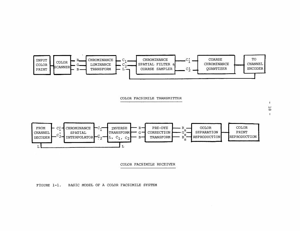
A preliminary model of the color facsimile system is shown in

figure 1. The transmitter consists of a color scanner with red, green,

and blue photodetectors and a chrominance luminance conversion transform,

followed by the chrominance spatial filter, coarse sampler, coarse

quantizer and encoder. At the receiver, the chromaticity components are

interpolated, and then inversely transformed with the luminance to red,

green, and blue signals which are pre-corrected for the non-ideal dyes

encountered in photographic or printing reproduction processes, and are

then simultaneously reproduced as red, green, and blue monochrome

separations.

A channel encoder, channel model, and channel decoder should be

inserted between the transmitter source encoder and receiver source

decoder, but this thesis only examines the source coding problem, and

so assumes an ideal channel. In television systems, a relatively poor

signal to noise ratio can be tolerated because the eye tends to

INPUT P CHROMINANCE. C1 CHROMINANCE

COLOR COLER G. LUMINANCE C2 SPATIAL FILTER &

PRINT B TRANSFORM L COARSE SAMPLER

COLOR FACSIMILE TRANSMITTER

FROM Ci CHROMINANCE C1 INVERSE R PRE-DYE R COLOR COLOR

CHANNEL u SPATIAL TRANSFORM G CORRECTION G S SEPARATION PRINT

DECODER C 2 INTERPOLATOR I 2 L, C1 , C2 B TRANSFORM B REPRODUCTION REPRODUCTION

O LL

COLOR FACSIMILE RECEIVER

BASIC MODEL OF A COLOR FACSIMILE SYSTEMFIGURE l-l.

- 19 -

integrate out the uncorrelated frame to frame noise, yielding a much

higher perceived signal to noise ratio. In facsimile, a single frame

is transmitted and may be reproduced hundreds of thousands of times in

newspapers. Therefore, nearly flawless transmission must be insured by

the channel coder since a strategically located error such as a spot

on a prominent politician's nose might necessitate retransmission of

the entire picture.

The interpel sample period for facsimile is 500 y sec or a few

thousand times the corresponding period for television. Therefore, in

addition to the operations of sampling, filtering, quantizing, and

packing there is sufficient time to perform complex chrominance trans-

forms with a high speed digital processor. Color coders for television

systems cannot afford this computational luxury, but color television is

an additive primary system and so many of the chrominance transforms

required to correct for subtractive dye systems encountered in facsimile

are unnecessary in television.

1.4 Summary

There has been much prior "knob-twiddling" by earlier researchers

of a limited number of color coding parameters so that several of these

(i.e., the chrominance spatial compression factor) can be set to a

reasonable value without further experimentation. Having specified these

basic parameters, the author is able to enter into new areas of color

coding research by developing algorithms which optimize color picture

quality given basic system architecture constraints and certain pre-

specified key parameter values.

- 20 -

This thesis takes the approach of attempting to work in the mathemat-

ically and physically defined colorimetric system in which the psycho-

physical data of most researchers is usually represented. The next

chapter examines various transforms of the chromaticity components in

the standard colorimetric color space.

II. Color

2.1:

2.2:

2.3:

2.4:

- 21 -

Space and Chrominance Quantization

Colorimetry

Color Space Representations and Transformations

Uniform Sensation Color Space

The Luminance Scaled Chromaticity (LSC) Transform

- 22 -

2.1 Colorimetry

The colorimetric design of a system to effectively process color

photographs must be based on the psychophysics of color vision and the

limitations of color photography. These disciplines must be inter-

related in evolving algorithms which efficiently compress and code color

pictures.

At the foundation of the psychophysics of color vision is the

Young-Helmholtz model of the eye which describes the retina as containing

three types of cone receptors, each with independent spectral sensation

(12,13)characteristics. The three cone responses peak in roughly the

red, green, and blue regions of the spectrum. The cone model is the

basis of colorimetry where any color sensation due to a stimulus with

a particular spectrum can be represented by three numbers, namely the

neural response of each cone. This gives rise to the phenomenon of

metamerism which occurs when two different spectral distributions

equally activate the three cone mechanisms. Thus an infinite number of

possible spectra, referred to as metamers, can be mapped by the eye into

the same color sensation.

The three dimensional nature of color vision is the basis for the

classic matching experiments where the radiances of three additively

projected primary light sources with spectral distribution, p (X), are

adjusted to match an unknown color source. The standard 1931 CIE

measurements used three narrowband spectral distributions centered at

700.0 nm, 546.1 nm and 435 nm to match narrowband regions along the

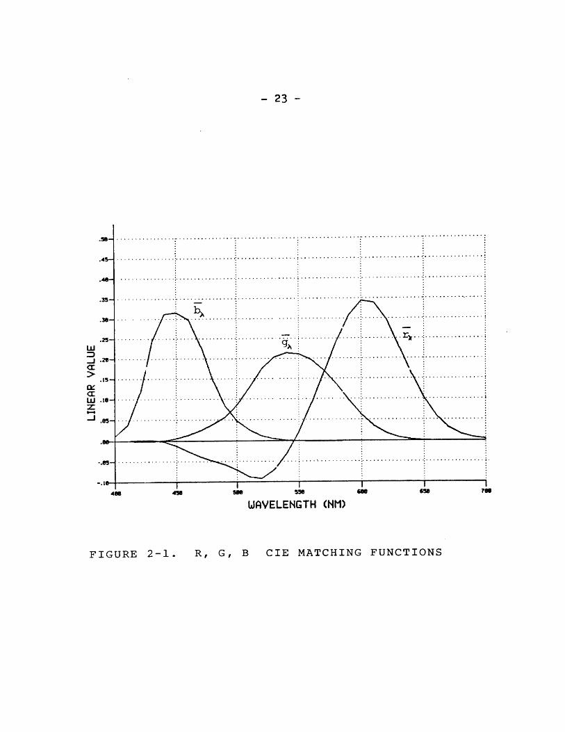
visible spectrum. Three color matching functions, x.(X), result fromJ

these measurements and are shown in figure 2-1. Negative values of the

- 23 -

o .30 - - -- - -. . . . ..--- --... --- -- - ---. .. .. -.--.-- - --.w-j .

20-

.-x .. . ..... .. .-.-- - - - - - - - - - - - - - - - - -

-.1.

wls

z

466 456 568 W56 m6 56

WAVELENGTH (NM)

FIGURE 2-1. R, G, B CIE MATCHING FUNCTIONS

- 24 -

matching function indicate that the match required the corresponding

primary light source to be added to the light being matched. Further

matching experiments show that any color stimulus, s( x), may now be

represented by the three chromaticity coordinates, R, G, B, which

represent the amount of each primary required to match the stimulus.

x.(X) = r(X), g(x), b(X)

X. = fx.(X) s(X) dA (2.1-1)

A X.= R, G, Be J

where A is the range of wavelengths of visual response, namely 380 toe

770 nanometers (nm).

Many sets of primaries other than the CIE standard primaries may

be used as the basis for specifying colors. The conversion to a new

primary system is detailed in Appendix I.

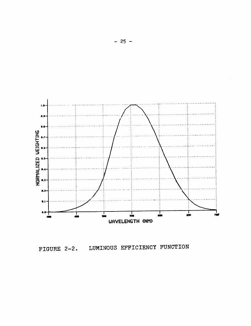
The luminance of a color is a measure of the apparent brightness.

Its value can be related to the radiant energy of a particular color by

the photopic luminosity curve which is a plot of luminous efficiency as

a function of wavelength. The luminosity function peaks in the green,

falls off in the red and decreases more sharply in the blue (figure 2-2).

Luminance is a very important parameter since its value must be trans-

mitted at full spatial resolution as the monochrome signal for black and

white system compatibility. Even in a strictly color system, the

luminance must be transmitted with maximum spatial resolution since the

eye has the greatest acuity for this visual component. (14)

From Grassmann's laws of additive color mixture it follows that the

luminance of an additive mixture of colors is a sum of the individual

(15)luminances. In particular for a proper set of tristimulus

- 25 -

in

. . .. . . . . . . . . .7 . . . . . . . . . . . . . . . . . . . . . . . . . .. . . . . . .

. . . . . . . . . . . . . . . . . . . . . . . . . . . . . . . . . . . . . . . . . . . . . . . .

. . . . . . . .. . . . . . .. . . . . . . . . . . . . . . . . . . . . . . . . . ..

. .. . . . . . . . . . . . .. . . . . . . . . . . . . . . . . . . . . . . . . . . . . . . . .

. . . . . . . . . . . . . . . .. . . . . . . . . . . . . . . . . . . . . . . . . . . . . . .

. . . . . . . . . . . . . . . .. . . . . . . . . . . . . . . . . . . . . . . . . . . .

................ 7 . . . . . . . . . . . . . . .. . . . . . . . . . . . . . . .

................ ......... .......................

................ . . . . . . . . . . . . . . . . . . . . . . . .. . . . . . . .

............. . . .. . . . . . . . . . . . .... .........

WAVELENGTH (NM)

LUMINOUS EFFICIENCY FUNCTION

z

L-0-

w:3

Cl

wN

40

........... ................. .........

................. .........................

........................... ... ..........

................. .........................

..................................... .....

... ........ ..... 7 .. . ..... ......... .. ......

. . . . . . . ... . . . . . . . . . . . . . . . . . . . . . . . . . . . . . . . .

. .. . .. .. .. . . .. .. 7 . .. . .... . .. .... .. .. .. . . . ..

............. . .... . . .. .. .. 7 .. ... .. . ... . ..

. . . . . . . . . . . . . . . . .. . . ... . . .. . . . . . . .7

FIGURE 2-2.

- 26 -

primaries, each of the color components contributes to luminance.

L = L R + L G + L B (2.1-2)r g b

Where each luminosity coefficient, L ., is the integral of the product of

the photopic luminosity curve and the primary distribution P. (X) over

wavelength.

L. = f L (X)P. (X)dl (2.1-3)

2.2 Color Space Representations and Transformations

Three dimensional color space can be described by a variety of

triads of parameters. A color can be specified by its red, green, and

blue coordinates in an infinite number of primary bases. In the case of

subtractive dyes, a color is completely described by knowing the amount

of the cyan, magenta, and yellow dyes, assuming a standard illuminant.

A more qualitative description of color results from specifying the

brightness, hue (common color name), and saturation (degree of color

purity ranging from white through pastel to a fully saturated mono-

chromatic color). The latter representation is noteworthy since now the

triad of parameters contains luminance as one term and the hue and

saturation pertain solely to the chrominance.

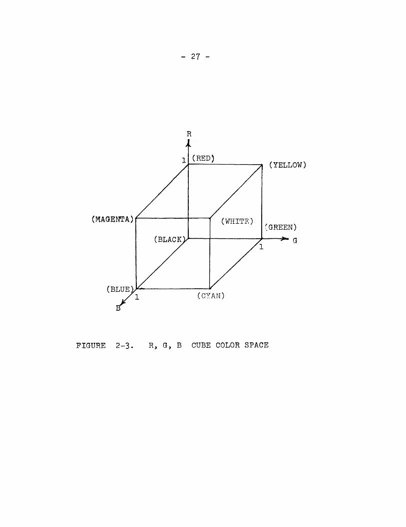
In any physical set of primaries, the range of synthesizable colors

can be represented as being contained in a unit cube (figure 2-3) by

normalizing maximum values of the primaries (i.e., to maximum white print

reflectance under specified illumination)

R G B =1 (2.2-1)max max max

- 27 -

R

(YELLO

(MAGENTA) (WHITE)(GREEN)

(BLUE),1 (CYAN)

R, G, B CUBE COLOR SPACE

W)

FIGURE 2-3.

- 28 -

If the primaries are each quantized to six bits, then over a quarter

of a million discrete possible colors lie within the cube. Perpendicular

axes, resulting in a cubic region of permissible colors, are used solely

as a convenience in drawing, since the exact angular relationships

between axes or even the shape of the color space is meaningless unless

some spatial distance metric can be defined as a function of the plotted

parameters.

It is also convenient to normalize the luminance, so that by 2.1-2

maximum luminance is unity.

L + L + L =1 (2.2-2)r g b

The brightest color in a reproduction system is usually the white point

and since this occurs when the three primaries are at their maximum

unity value, whenever the primaries have the same value, the color

specified will be achromatic.

at achromatic points: R = G = B = L (2.2-3)

The primaries can be linearly transformed to a new coordinate system,

where one of the new components is luminance. The two remaining

components are measures of chrominance.

L R

Cl = G (2.2-4)

C ~~ B

This linear transform must be invertible so the C and C2 must be in-

dependent of L and have zero luminance. In figure 2-4 the transformed

cubic primary space is shown in the new L, C1, C2 space, where the

- 29 -

Y

R

Lr

Cl

(WHITE)

C

C2

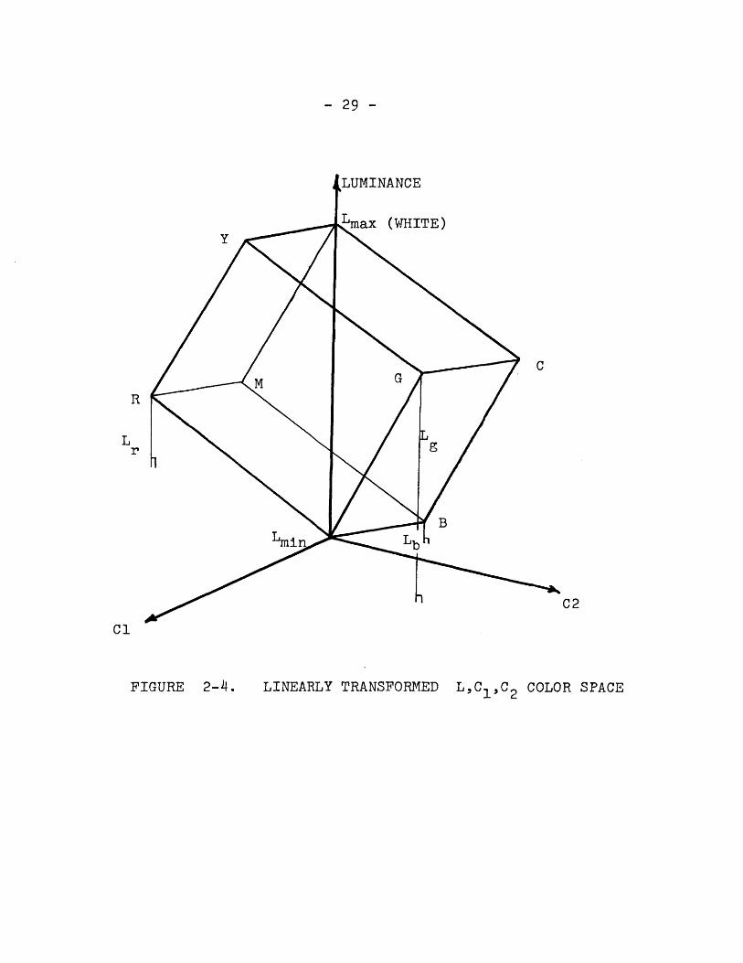
LINEARLY TRANSFORMED L,C ,C 2 COLOR SPACEFIGURE 2-4.

- 30 -

luminosity of any point in the space is the distance from the point to

the plane formed by the C 1 and C2 axes along a line parallel to the L

axis. Thus the exact location of the C -C2 plane is specified by the

L , L , L distances it must be located from the R , G , and Br g b max max max

vertices of the parallelpiped. The NTSC color television system uses

this type of chrominance transformation.

The mapping from R, G, B space to L, C1, C2 space is inefficient

since the parallelpiped volume spanned by the maximum and minimum L, C1 ,

C2 values is larger than the transformed R, G, B parallelpiped volume of

real colors. Thus quantization of the L, C 1 , C2 axes yields a volume

of color code word boxes where a large number of boxes do not represent

a valid color. This is a direct consequence of constraining the space

by the R,G,B cube and using luminance as one of the coordinates, thereby

placing boundaries on the gamut of realizable chrominance values which

vary as a function of luminance.

2.3 Uniform Sensation Color Space

Ignoring statistical weighting, the L, C 1, C2 -coding space will be

most efficiently quantized if equal quantum steps along the coordinates

produce nearly equal visual sensations. In the case of luminance

quantization, much experimentation(16, 17) has revealed that a modified

logarithmic function, L, produces the most uniform quantization since it

evenly distributes perceived picture noise and contour artifacts over

the entire tone scale.

Log (l + aL)L =Log (1 + a)

- 31 -

where the companding shape factor a has an optimum value found

experimentally to lie between .01 and .1 depending on the desired shadow

detail in the picture.

As a first step in obtaining a uniform chrominance scale (UCS)

sensation plane, researchers determined the just noticeable differences

(JND) of chrominance changes for various colors and plotted the loci of

these JND points around the particular color point in a bilinear

chromaticity plane. (18)

A general bilinearly transformed chromaticity plane can be set up

by first linearly transforming the CIE coordinates.

Cl RC2 = [T] G (2.3-2)

C3 B

The conical projection of points in the Cl, C2, C3 space onto the

Cl + C2 + C3 = 1 plane in that space results in three chromaticity

coordinates, cl, c2, c3.

cl = Cl c2 C2Cl + C2 + C3 Cl + C2 + C3

(2.3-3)

C3c3 = C3 cl + c2 + c3 = 1

C1 + C2 + C3

The chromaticity coordinates cl, c2, c3 are relative values and are

therefore independent of the absolute value of the color coordinates

Cl, C2, C3. Since chrominance has only two degrees of freedom, choosing

cl and c2 as the independent variables projects points on the

Cl + C2 + C3 = 1 plane onto the cl, c2 plane.

- 32 -

The CIE-UCS coordinates u and v may be defined in terms of the R,G,B

CIE coordinates:

u R+ uG + uB v R+ vG +vbBU r g b r b (2.3 -4)

s R + s G + s B s R + s G + s Br g b r g b

Appendix II shows how 2.3-4 and 2.3-5 may be inverted to yield:

R = L(r u + r v + a)/D(u,v) where a,b,c,r ,r ,g ,g ,b ,b ,d ,d ,d

G = L(g u + g v + b)/D(u,v) are constants.u V (2.3-5)

B = L(b u + b v + c)/D(u,v) D(u,v) = d u +d v + du v u v

For most chrominance coordinates (cl, c2) the JND loci are ellipses

which greatly vary in size, degree of elongation, and angle of rotation.

True UCS transformation would map these JND ellipses into equidiameter

circles. The 1960 CIE-UCS transform'is a particular bilinear transform

of the tristimulus coordinates which creates a chrominance plane that

is a reasonably close approximation to the ideal UCS chrominance plane.

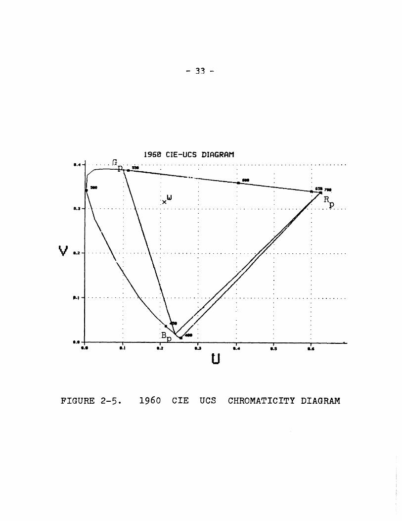
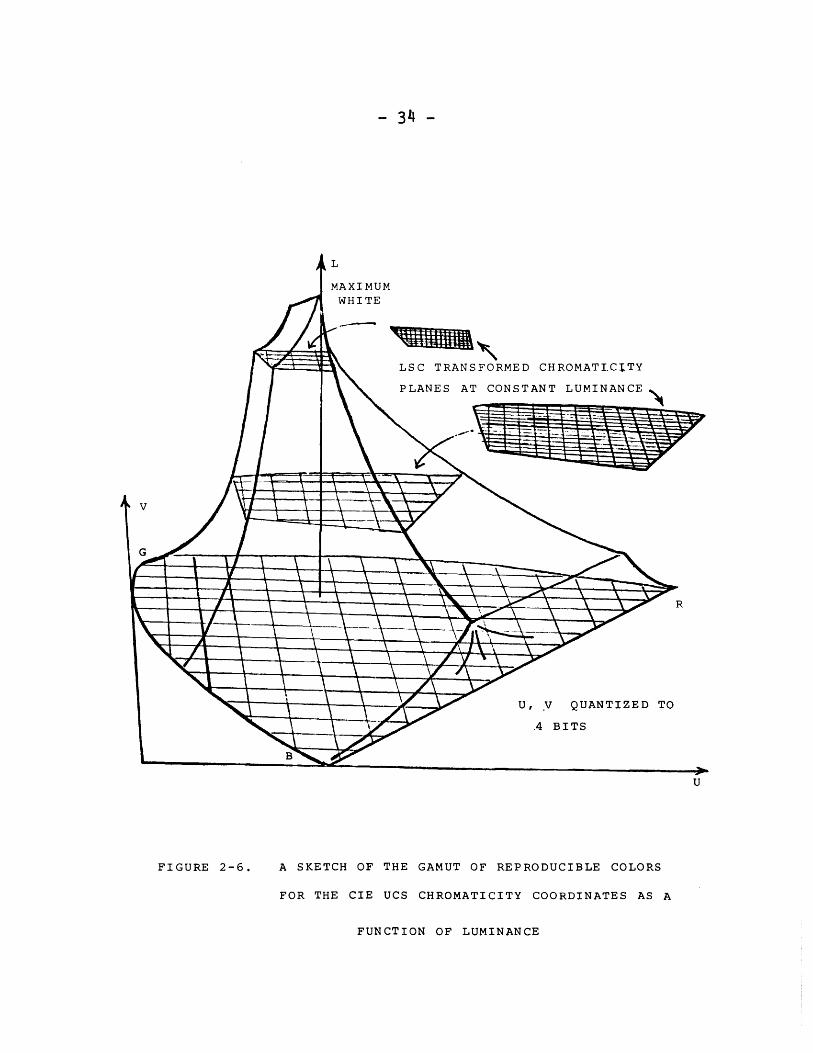
The widely accepted 1960 CIE-UCS chromaticity plane is illustrated

in figure 2-5, with spectrum locus and white point, as well as the

triangle whose vertices are the CIE RGB primaries. A color space con-

sisting of the luminance and UCS chromaticity coordinates is sketched

in figure 2-6. Compared to the linearly transformed parallelpiped

L, Cl, C2 space, there are much fewer wasted code words at low luminance

levels. However, uniform quantization of the Cl and C2 coordinates

results in very inefficient use of available chrominance code words at

moderate luminance levels.

- 33 -

1960 CIE-UCS DIAGRAM.. . . . .. .... .. . . . .

653 ?UA

R. P..

/ . . .. . . .. . .

ILI; ... . .

8.3 8.4

U

1960 CIE UCS CHROMATICITY

.xA

V 3.2

3..0. 6.2

. . . . . . . . . .

..... ....

.................

FIGURE 2-5.0 DIAGRAM

L

MAXIMUMWHITE

LSC TRANSFORMED CHROMATI.CITY

PLANES AT CONSTANT LUMINANCE

R

U, Y QUANTIZED TO

.4 BITS

U

FIGURE 2-6. A SKETCH OF THE GAMUT OF REPRODUCIBLE COLORS

FOR THE CIE UCS CHROMATICITY COORDINATES AS A

FUNCTION OF LUMINANCE

- 34 -

- 35 -

2.4 The Luminance Scaled Chromaticity (LSC) Transform

In all common color reproduction systems, the gamut of chromaticities

is constrained to lie inside a region in the UCS plane. In a typical

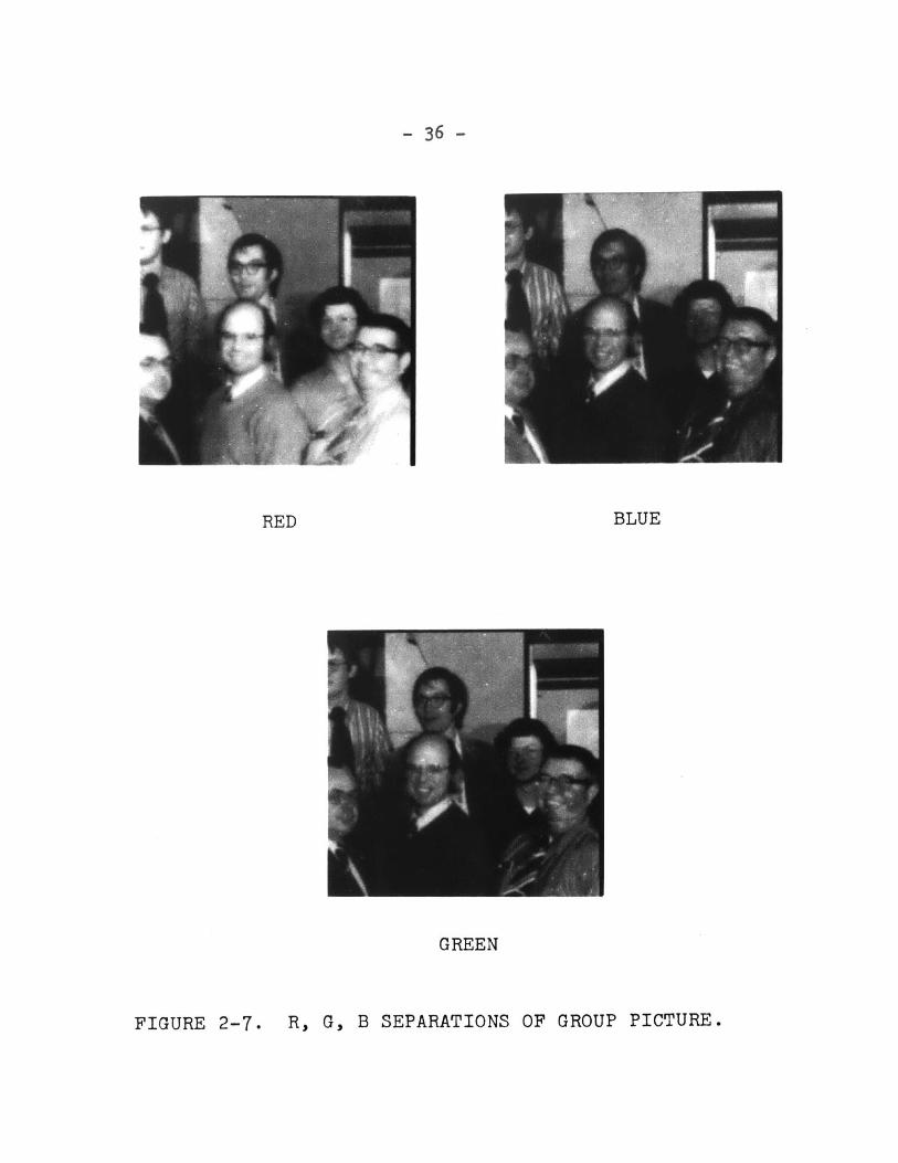
picture the R, G, B primaries are statistically dependent. Most colors

in a typical portrait or natural scene are achromatic or desaturated.

Since the primaries must be nearly equal for desaturated colors, it

follows that they are highly correlated with each other. This can be

intuitively seen by observing the similarity of the red, green, and blue

separations of a color picture (figure 2-7).

Transformation of the primary coordinates to a luminance and two

independent UCS chrominance components results in a significant reduction

of the inter-component correlations (figure 2-8).

When luminance is used as one of the three components, it has been

shown that it restricts the values of the chrominance components, u and

v (figure 2-6). For very low luminance levels, the R, G, B primaries

may take on any ratio of values and u and v may assume any value within

the chrominance plane primary triangle. When the luminance is increased

above Lb the value of the blue primary luminosity coefficient, u and v

are then restricted from taking on values in the saturated blue region of

the chrominance plane. As the luminance is further increased, the area

of permissible u and v values decreases until the maximum luminance is

reached where the only possible chromaticity value is the achromatic point.

A series of constant luminance loci is plotted in figure 2-9. The

loci contain the gamut of reproducible colors with the constraints of

equations 2.1-3, 2.2-1, 2.2-2, and 2.3-4. Starting at the maximally

saturated red value for a particular fixed luminance, the blue component

- 36 -

RED BLUE

GREEN

R, G, B SEPARATIONS OF GROUP PICTURE.FIGURE 2-7.

- 3' -

L

FIGURE 2-8.

Cl

C2

1. C2 COMPONENTS OF GROUP PICTUREL, CL. C

- 38 -

1960 CIE-UCS DIAGRAM

seu

. . . . . . . . . . . . . . . . . . . . .. ...

L=.2

-. - -. - . . . . . . ..

'.4 P.5 9.6

U

FIGURE 2-9. LOCI OF CONSTANT LUMINANCE ON UCS

CHROMATICITY DIAGRAM

9.4

0.3

V 9.2

.1 - -. .- - - ..- -

0.. 6.1

- 39 -

is increased and the red decreased until the most saturated blue-magenta

is reached. Then the green is increased and the red further decreased,

moving the loci to maximally saturated blue-cyan. By increasing the

green and decreasing the blue, the maximally saturated green point is

reached. Finally, the green is decreased as the red increases back to

its maximum possible value. These constant luminance planes are sketched

as volume in color space in figure 2-6.

L/L L LH = H H for H = R, G, B (2.4-1)max 1L

1 L LHH

Another way of viewing the restriction of u and v values as a

function of luminance is to realize that in a three primary color space

(such as a subtractive photographic dye process, additive phosphor

television system, or even the eye), the luminance component contains

much chromaticity information and has been shown to be correlated with

chrominance. (19) Luminance is not highly correlated to low luminosity

components such as blue, but is very highly negatively correlated with

the relative blue component.

If the u and v coordinates are quantized, then even at very low

luminance levels, chromaticity quantization is not too efficient since

the right triangle base of figure 2-9 results in an area where only half

of the possible number of codewords is utilized. The real colors lie in

a horseshoe-shaped spectrum locus contained inside the triangular base

and the gamut of reproducible colors lies inside the horseshoe. Thus

even at the lowest luminance levels, simple quantization of u and v is

less than 50 percent efficient. As the luminance increases the number

-40-of valid chrominance code words is drastically reduced. Similar effects

have been noted in the Munsell color system as value is increased. (20)

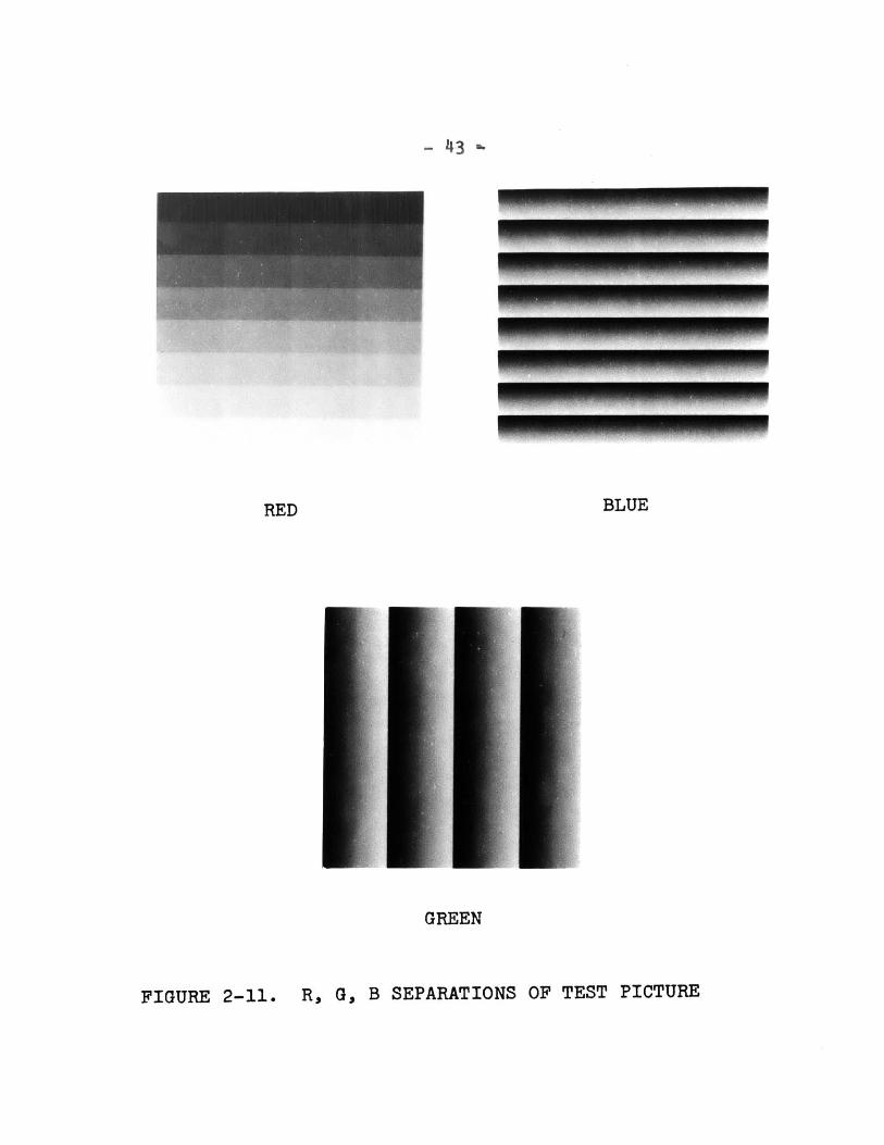
To facilitate the development of the color coding algorithms, it is

useful to monitor the effects of quantization and filtering on the red,

green, and blue separations. The test pattern separations of figure 2-11

generate the full gamut of colors in the system by reproducing over

100,000 different triads of red, green, and blue values in the 256 pel by

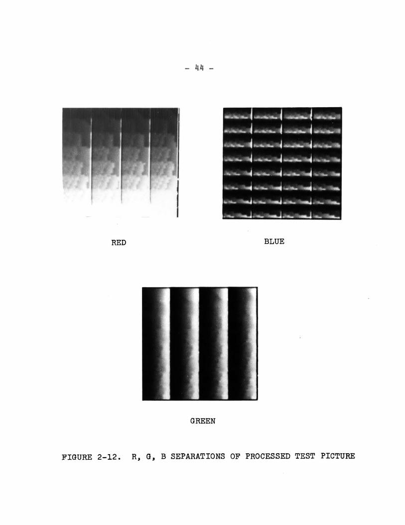
256 line test pictures. The quantization contour artifacts resulting

from coarse quantization of each chrominance component to four bits

are shown in figure 2-12. These artifacts are most severe at high

luminance levels. If u and v are each uniformly quantized to 16 levels,

then at luminance levels above L r, only 50 color boxes would be available

to represent realizable colors.

In a typical natural scene, most of the chrominance values are

clustered near the white point with a few more saturated colors lying

along certain dominant hue lines which are different for each particular

picture. The frequency of occurrence of Cl and C2 values which have been

coarsely quantized to four bits (16 levels) each are listed in Table 2-1

for the group picture of figure 6-lA. Even for this rather colorful

picture the Cl and C2 values are significant only near the white point.

Thus the desaturated colors, many of which often occur at high

luminance levels as pastels, constitute the majority of colors in many

pictures. Accurate reproduction of pale skin tones is crucial for

achieving acceptable subjective color picture quality. As previously

discussed, however, the number of available chrominance boxes is

very small for these important pastel colors, resulting in objectionable

quantization contours due to roundoff errors.

FREQUENCY OF OCCURRENCE OF Cl-C2 VALUES FOR THE GROUP

Cl

15 - 0 0 0 0 29 58 9 0 0 0 0 0 0 0 0 0

14 - 0 0 0 39 201 483 117 458 279 60 5 25 2 0 0 0

13 - 0 0 0 18 442 1106

12 - 0 0 0 826 1169 318

286 135 442 421 23 49 10 0 0 0

40 6 9 2 0 0 0 0 0 0

11 - 0 0 0 211 83 11 0 0 0 0 0 0 0 0 0 0

10 - 0 0 0 69 63 0 0 0 0 0 0 0 0 0 0 0

9 - 0 0 0 402 95 0 0 0 0 0 0 0 0 0 0 0

8 - 0 127 0 0 0 0 0 0 0 0 0 0 0 0 0 0

7 - 0 63 0 0 0 0 0 0 0 0 0 0 0 0 0 0

6 -0 0 0 0 0 0 0 0 0 0 0 0 0 0 0 0

5 -0 0 0 0 0 0 0 0 0 0 0 0 0 0 0 0

4 -1 0 0 0 0 0 0 0 0 0 0 0 0 0 0 0

3 -0 0 0 0 0 0 0 0 0 0 0 0 0 0 0 0

2 -0 0 0 0 0 0 0 0 0 0 0 0 0 0 0 0

1 -0 0 0 0 0 0 0 0 0 0 0 0 0 0 0 0

0 -0 0 0 0 0 0 0 0 0 0 0 0 0 0 0 0

0 1 2 3 4 5 6 7 8 9 10 11 12 13 14 15 C2

TABLE 2-l. PICTURE

- 42 -

L LSC Cl

LSC C2

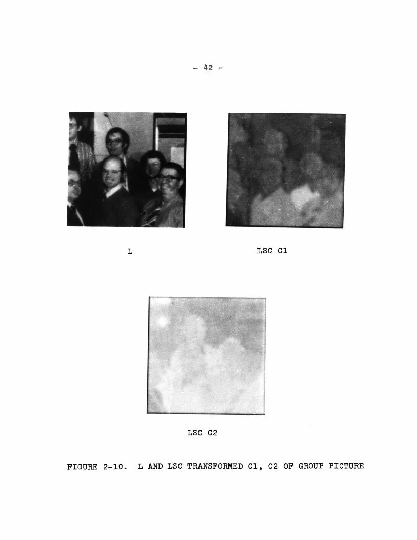
FIGURE 2-10. L AND LSC TRANSFORMED Cl, C2 OF GROUP PICTURE

- 43 a-

RED BLUE

GREEN

FIGURE 2-11. R, G, B SEPARATIONS OF TEST PICTURE

..........

.... ......

- 44 -

P P P

RED BLUE

GREEN

FIGURE 2-12. R, G, B SEPARATIONS OF PROCESSED TEST PICTURE

-45-

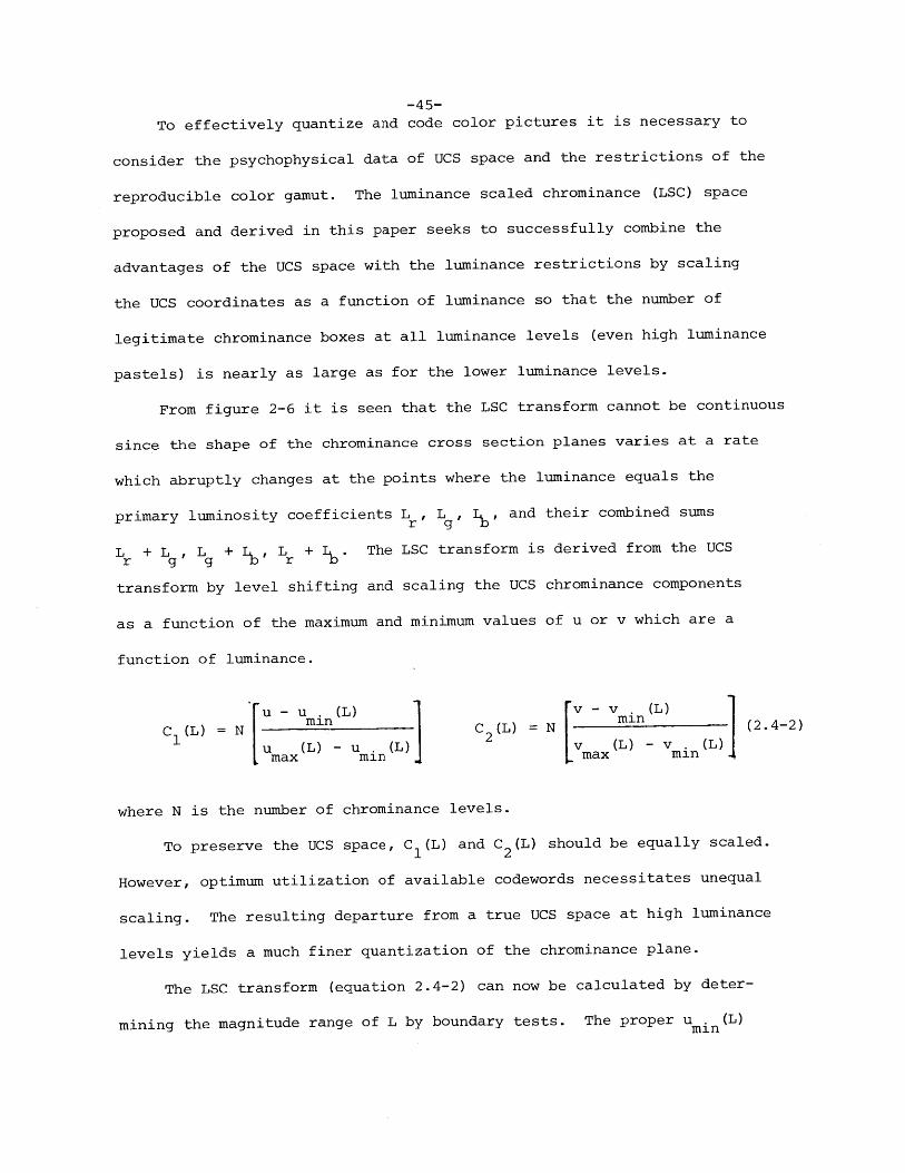
To effectively quantize and code color pictures it is necessary to

consider the psychophysical data of UCS space and the restrictions of the

reproducible color gamut. The luminance scaled chrominance (LSC) space

proposed and derived in this paper seeks to successfully combine the

advantages of the UCS space with the luminance restrictions by scaling

the UCS coordinates as a function of luminance so that the number of

legitimate chrominance boxes at all luminance levels (even high luminance

pastels) is nearly as large as for the lower luminance levels.

From figure 2-6 it is seen that the LSC transform cannot be continuous

since the shape of the chrominance cross section planes varies at a rate

which abruptly changes at the points where the luminance equals the

primary luminosity coefficients Lr , L , L, and their combined sums

L + L , L + Lb, L + Lb. The LSC transform is derived from the UCSr g g b r

transform by level shifting and scaling the UCS chrominance components

as a function of the maximum and minimum values of u or v which are a

function of luminance.

u - u v - (L)

C (L) = N min C(2)(L) = N [ in (2.4-2)

l u L) -u . L) v (L) v V CL)max min max min

where N is the number of chrominance levels.

To preserve the UCS space, C 1 (L) and C 2 (L) should be equally scaled.

However, optimum utilization of available codewords necessitates unequal

scaling. The resulting departure from a true UCS space at high luminance

levels yields a much finer quantization of the chrominance plane.

The LSC transform (equation 2.4-2) can now be calculated by deter-

mining the magnitude range of L by boundary tests. The proper umin (L)

and u (L) functions are first evaluated and then C (L) and C (L) canmax 1 2

be derived. The minimum and maximum u and v are shown (in Appendix III)

to be of the form:

min u

or or = [a + bL]/[c + L] (2.4-3)

max v

so only six constants (at most) need be stored for each range of L values.

The inverse LSC transform is of the same form and uses the same coef-

ficients.

The LSC transform can be simplified by fixing the transform scaling

and shifting parameters to their values at L for luminance levelsg

greater than L . With this limitation, the pastel colors will still

have much greater chrominance resolution than with just the UCS transform,

and limiting the scaling avoids the problem of scaling up a vanishingly

small area of valid chrominance values by very large factors at large

luminance values. Figure 2-6 illustrates the substantial increase in

reproducible chrominance codeword boxes in the LSC transformed coordinates

at high luminance levels.

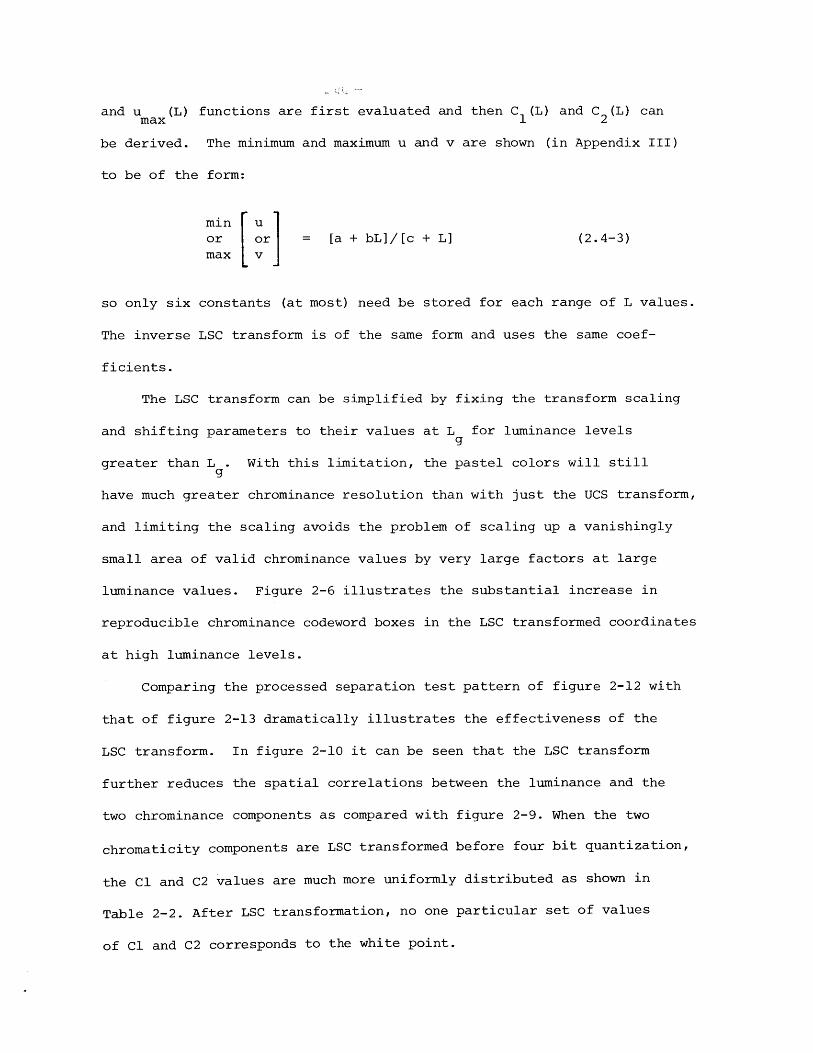
Comparing the processed separation test pattern of figure 2-12 with

that of figure 2-13 dramatically illustrates the effectiveness of the

LSC transform. In figure 2-10 it can be seen that the LSC transform

further reduces the spatial correlations between the luminance and the

two chrominance components as compared with figure 2-9. When the two

chromaticity components are LSC transformed before four bit quantization,

the Cl and C2 values are much more uniformly distributed as shown in

Table 2-2. After LSC transformation, no one particular set of values

of Cl and C2 corresponds to the white point.

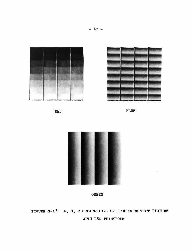
RED BLUE

GREEN

FIGURE 2-13. R, G, B SEPARATIONS OF PROCESSED TEST PICTURE

WITH LSC TRANSFORM

4V I j

- 47 -

, '- I - .- w . I . 1w. I

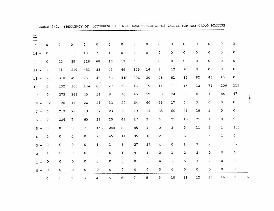
TABLE 2-2. FREQUENCY OF OCCURRENCE OF LSC TRANSFORMED C1-C2 VALUES FOR THE GROUP PICTURE

Cl

15 - 0 0

14 - 0 0

13 - 0 23

12 - 1 11

11 - 25

10 - 0

318

0 0 0 0 0 0 0 0 0 0 0 0 0 0

11 18 7 1 0 0 0 0 0 0 0 0 0 0

39 318 68 13 12 0 1 0 0 0 0 0 0 0

219 483 35 43 49 129 14 8 12 20 0 0 0 0

496 75 46 53 448 306 20 26 61 35 82 43 14 0

132 165 134 60 27 21 45 19 11 11 15 13 74 206 111

9 - 0 273 261 45 14 8 36 45 59 33 24 8 4 7 85 47

8 - 92 120 17 26 24 13 22 64 60 36 17 4 3 0 0 0

7 - 0 213 79 19 37 23 30 19 24 35 60 41 19 1 0 0

6 - 0 334 7 60 28 20 42 17 3 4 22 18 25 1 0 0

5 - 0 0 0 7 158 244 8 85 1 0 3 9 11 2 1 156

4 - 0 0 0 0 2 45 14 35 10 2 1 6 1 3 1 2

3 -0 0 0 0 1 1 3 27 17 4 0 1 2 7 1 32

2 1 0 0 0 0 0 1 9 1 0 1 2 2 0 0 0

1 0 0 0 0 0 0 0 01 0 4 2 5 3 2 0 0

0 -0 0 0 0 0 0 0 0 0 0 0 0 0 0 0 0

0 1 2 3 4 5 6 7 8 9 10 11 12 13 14 15 C2

00

THE GROUP PICTUREOCCURRENCE OF LSC TRANSFORMED Cl-C2 VALUES FORTABLE 2-2. FREQUENCY OF

-49-

III. The Chrominance Spatial Filtering Process

3.1: The Psychophysical Basis for Chrominance Spatial Filtering

3.2: The Overall Filter Function

3.3: Luminance Filtering for the LSC Transform

-50-

3.1 The Psychophysical Basis for Chrominance Spatial Filtering

The ability to compress the color components of a picture is

primarily due to the eye's lower spatial acuity for chrominance detail

relative to the luminance acuity. Phrased another way, the lower spatial

bandwidth of chrominance in the eye implies a higher degree of spatial

correlation in the eye for the chrominance components. In addition, early

(2 1-24)work in the area suggests that the trichromatic visual system

becomes dichromatic as the size of a color patch is decreased. For small

patches the eye appears to behave as if it were tritanopic (i.e., exhibits

blue color blindness). The axis in the chromaticity diagram for the

highest resolution was determined to be along the orange-red cyan axis. (25)

From measurements of the chromatic modulation transfer function of

the eye, it has been found that for color spatial variation the high

frequency response falls off faster than in the case of luminance.(26)

This suggests that the effective color receptor area is larger than the

luminance receptor area. In addition, no Mach Band effect is noted at

heterochromatic, equi-luminance transitions implying that the retinal

color mechanism is not spatially organized as Kuffler units as is the

(27)luminance system. Supporting these observations are chromatic

modulation transfer function data which indicate that, unlike the

luminance case, there is no low spatial frequency fall-off or peaking

noted in tests with colored sinewave gratings. (28)

The first subjective experiments on chrominance filtering were

performed by the NTSC.(25) An initial experiment describes testing

various subjects with many color pictures, in which the luminance had

full resolution, but the R, G and B horizontal resolution could be de-

creased by a factor of four, before any substantial picture degradation

-51-(29) (30)

was noted. An experiment by Baldwin was the first to demonstrate

two dimensional color filtering by defocusing separately the blue, red

and green separations with an additive projector until subjective de-

gradation was noticed. This acuity for defocus was found to be almost

the same for green as for luminance (white). The red image could be

defocused much more than the green without noticeable degradation.

Furthermore, the blue could be completely defocused within the limits of

the projector with no perceived effects. These measurements, however,

are not a result of strict chrominance filtering, and the blue defocusing

for high luminance color pictures can be explained by the chromatic

aberration in the eye. The first series of experiments which spatially

filtered and coarse sampled the chrominance in two dimensions was done by

Gronemann, who obtained good quality pictures by spatially sampling the

chrominance at 1/20 the resolution of the luminance. (10)

Color television makes use of the higher resolution of the chromat-

icity components in the orange-cyan direction by choosing one chrominance

component (the I signal) in this direction to have three times the band-

width of the other perpendicular chrominance component (Q signal). Most

commercial receivers do not have the expensive circuitry to detect the

full bandwidth I signal and so for all practical purposes I and Q signals

have similar spatial resolution. In the facsimile system, the compression

ratio is not appreciably improved if the two chromaticity components are

unequally filtered. In addition, Chapter Four discusses linear transforms

performed on the coarsely sampled, filtered chromaticity components,

requiring that they be identically coarse sampled.

-52-

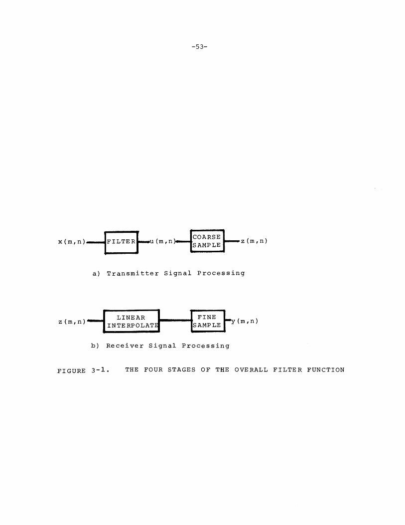
3.2 The Overall Filter Function

There are actually four distinct digital processing operations which

give rise to the overall filter function (figure 3-1). First, at the

transmitter, the value of the chrominance components at each pel (with

horizontal and vertical position indices m,n), x(m,n), is given a

weight, h(m,n), and summed, yielding a filtered output point, w(m,n).

This superposition method of filtering is the easiest to implement and

is feasible if the filter requirements are not too stringent.

N N

w(m,n) = E x(m + j, n + k) h(j,k) (3.2-1)

j=1 k=l

For isotropic systems, hexagonal sampling with circularly symmetric

filter functions is preferred. However, a rectangular sample structure

permits the use of easily implemented filters which are separable in the

vertical and horizontal directions.

h(j,k) = h (j) h 2(k) (3.2-2)

For a separable filter function, 3.2-1 becomes:

N N (3.2-3)

w(m,n) = E h2 (k) E h (j) x(m + j, n + k)

k=l j=l

The vertical and horizontal resolutions of the facsimile system

are nearly equal and since the eye is basically spatially isotropic, the

filters should be the same in both the horizontal and vertical directions.

h1 (j) = h 2 (j) = h(j) (3.2-4)

-53-

x (m,n) uFITERm (m, n OSA E z (m,n)

a) Transmitter Signal Processing

z(m,n) LINEAR FINE y(m,n)z~in~n] SAMPLE y'nJnINTERPOLA AML E

b) Receiver Signal Processing

THE FOUR STAGES OF THE OVERALL FILTER FUNCTIONFIGURE 3-l.

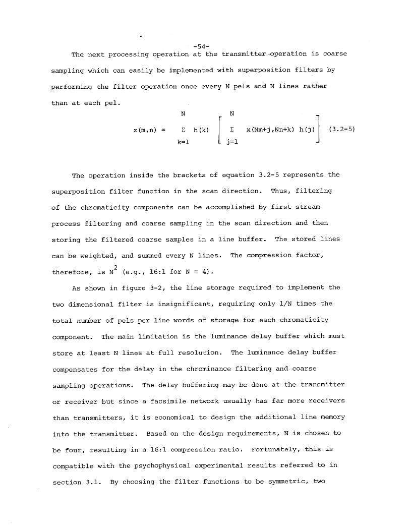
-54-The next processing operation at the transmitter-operation is coarse

sampling which can easily be implemented with superposition filters by

performing the filter operation once every N pels and N lines rather

than at each pel.

N N

z(m,n) = E h(k) E x(Nm+j,Nn+k) h(j) (3.2-5)

k=l [ j=l -

The operation inside the brackets of equation 3.2-5 represents the

superposition filter function in the scan direction. Thus, filtering

of the chromaticity components can be accomplished by first stream

process filtering and coarse sampling in the scan direction and then

storing the filtered coarse samples in a line buffer. The stored lines

can be weighted, and summed every N lines. The compression factor,

therefore, is N2 (e.g., 16:1 for N = 4).

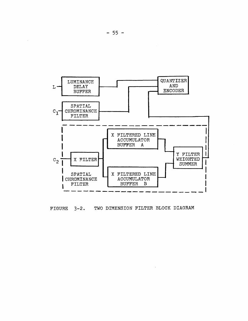
As shown in figure 3-2, the line storage required to implement the

two dimensional filter is insignificant, requiring only 1/N times the

total number of pels per line words of storage for each chromaticity

component. The main limitation is the luminance delay buffer which must

store at least N lines at full resolution. The luminance delay buffer

compensates for the delay in the chrominance filtering and coarse

sampling operations. The delay buffering may be done at the transmitter

or receiver but since a facsimile network usually has far more receivers

than transmitters, it is economical to design the additional line memory

into the transmitter. Based on the design requirements, N is chosen to

be four, resulting in a 16:1 compression ratio. Fortunately, this is

compatible with the psychophysical experimental results referred to in

section 3.1. By choosing the filter functions to be symmetric, two

- 55 -

L DELABUFF:

SPATIC- CHROMIN

FILTE

F2

FIGUJ

SPATIAL X FILTERED LINECHROMINANCE ACCUMULATORFILTER BUFFER B

TWO DIMENSION FILTER BLOCK DIAGRAMRE 3-2.

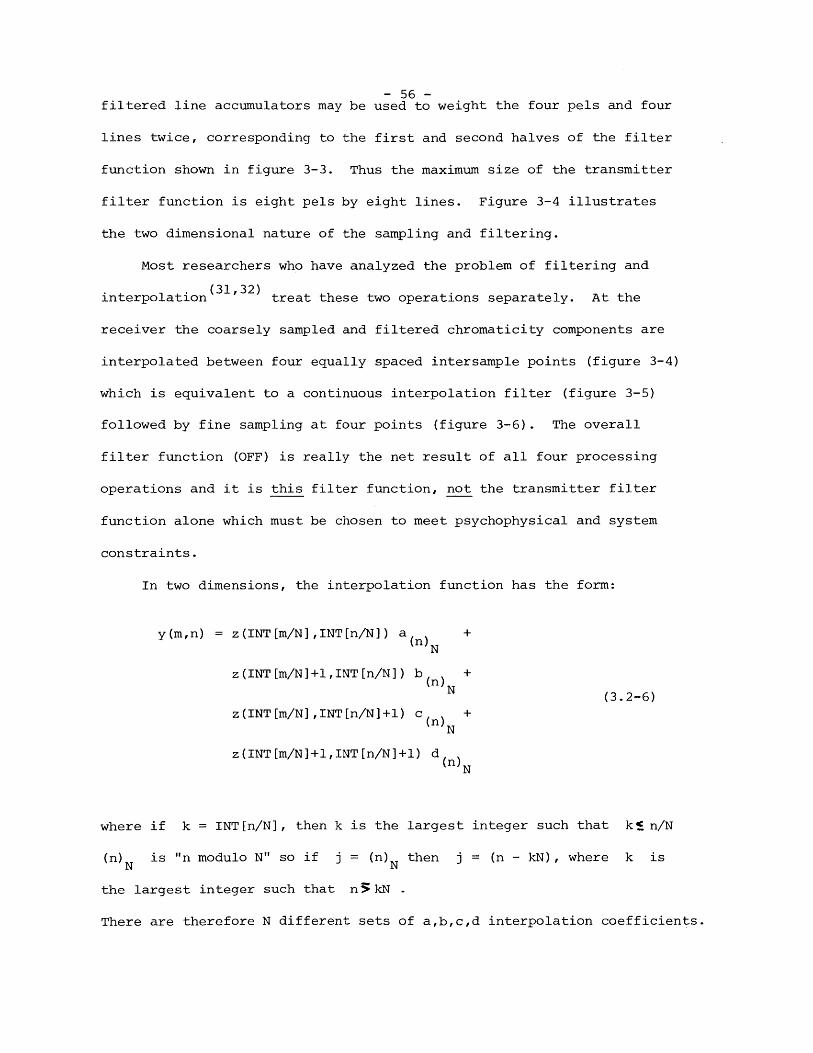
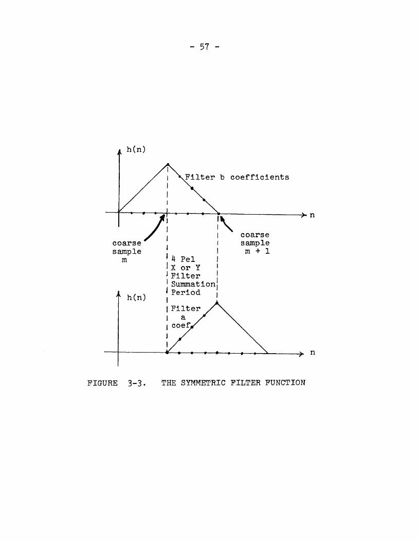
- 56 -filtered line accumulators may be used to weight the four pels and four

lines twice, corresponding to the first and second halves of the filter

function shown in figure 3-3. Thus the maximum size of the transmitter

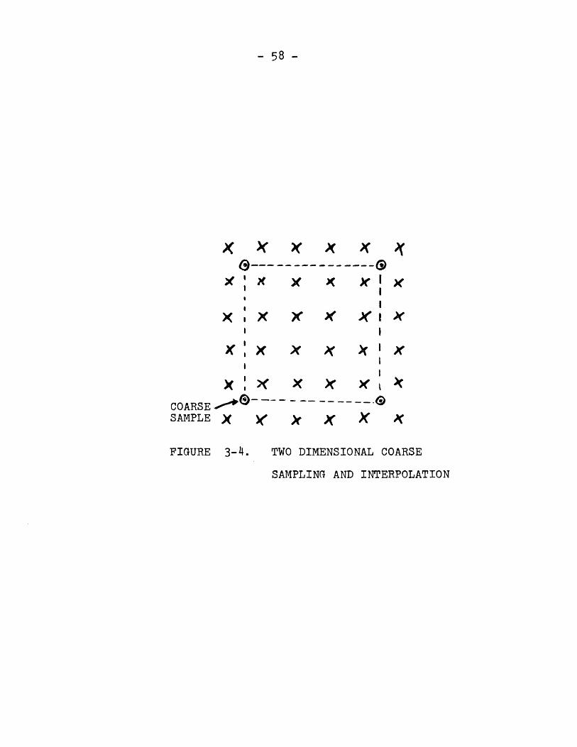
filter function is eight pels by eight lines. Figure 3-4 illustrates

the two dimensional nature of the sampling and filtering.

Most researchers who have analyzed the problem of filtering and

interpolation(31,32) treat these two operations separately. At the

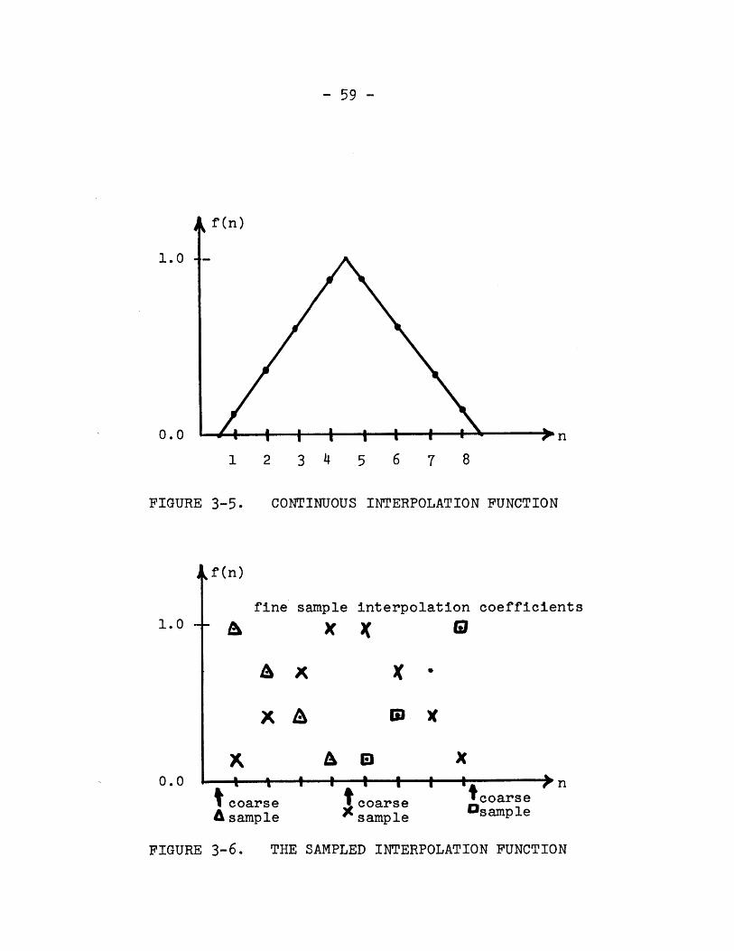
receiver the coarsely sampled and filtered chromaticity components are

interpolated between four equally spaced intersample points (figure 3-4)

which is equivalent to a continuous interpolation filter (figure 3-5)

followed by fine sampling at four points (figure 3-6). The overall

filter function (OFF) is really the net result of all four processing

operations and it is this filter function, not the transmitter filter

function alone which must be chosen to meet psychophysical and system

constraints.

In two dimensions, the interpolation function has the form:

y(m,n) = z(INT[m/N],INT[n/N]) a (n) +

z(INT[m/N]+l,INT[n/N]) b +(N (3.2-6)

z(INT[m/N],INT[n/N]+l) c +(n)N

z(INT[m/N]+l,INT[n/N]+l) d(n)

where if k = INT[n/N], then k is the largest integer such that kj n/N

(n) is "n modulo N" so if j = (n)N then j = (n - kN), where k is

the largest integer such that n5kN .

There are therefore N different sets of a,b,c,d interpolation coefficients.

- 57 -

h(n)

b coefficients

coarsesamplem

h(n)

FIGURE 3-3.

coarsesample

S m + 14 PelX or YFilterSummation,Period

IFilterIacoef

THE SYMMETRIC FILTER FUNCTION

- 58 -

K X X K KiX~ x

COARSESAMPLEX ){ g A'

FIGURE 3-4. TWO DIMENSIONAL COARSE

SAMPLING AND INTERPOLATION

- 59 -

f (n)

n

2 3 4 5 6 7 8

CONTINUOUS INTERPOLATION FUNCTION

fine sample interpolation coefficients

X X (a&

'C a

x a I IE

tcoarsesample

tcoarse0 sample

1.0 -

0.0

1

FIGURE 3-5.

0.0

I coarseAsample

THE SAMPLED INTERPOLATION FUNCTION

0 a 1.

4k f (n)

FIGURE 3-6.

- 60 -

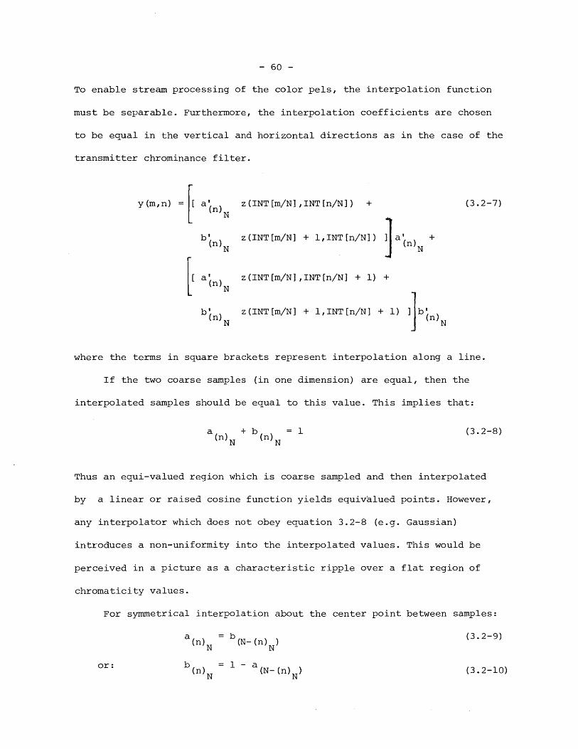
To enable stream processing of the color pels, the interpolation function

must be separable. Furthermore, the interpolation coefficients are chosen

to be equal in the vertical and horizontal directions as in the case of the

transmitter chrominance filter.

y(m,n) =[ a'() z(INT[m/N],INT[n/N]) + (3.2-7)

b '(n) z(INT[m/N] + 1,INT[n/N]) ] ' +(n)N la )

[ a' z(INT[m/N],INT[n/N] + 1) +

b' z(INT[m/N] + 1,INT[n/N] + 1) ]jb')(n) Nn

where the terms in square brackets represent interpolation along a line.

If the two coarse samples (in one dimension) are equal, then the

interpolated samples should be equal to this value. This implies that:

a + b = 1 (3.2-8)(n) (n)N N

Thus an equi-valued region which is coarse sampled and then interpolated

by a linear or raised cosine function yields equivalued points. However,

any interpolator which does not obey equation 3.2-8 (e.g. Gaussian)

introduces a non-uniformity into the interpolated values. This would be

perceived in a picture as a characteristic ripple over a flat region of

chromaticity values.

For symmetrical interpolation about the center point between samples:

a = b (3.2-9)(n) (N- (n) )

N N

or:b(n) N=1-a(N- (n) N) (3. 2-10)

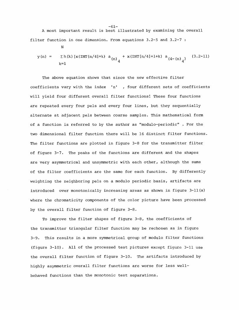
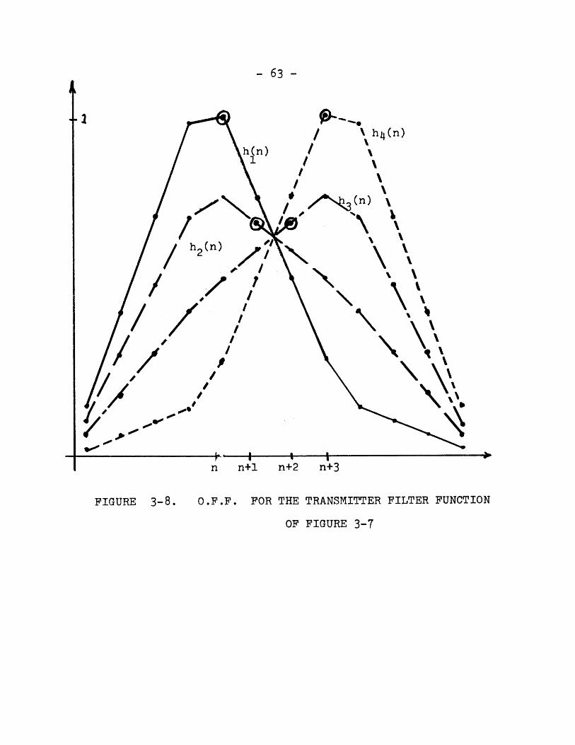
-61-A most important result is best illustrated by examining the overall

filter function in one dimension. From equations 3.2-5 and 3.2-7

N

y(n) = Eh(k)[x(INT[n/4]+k) a + x(INT[n/41+l+k) a( 4 () (3.2-11)(n) (-n

k=l

The above equation shows that since the new effective filter

coefficients vary with the index 'n' , four different sets of coefficients

will yield four different overall filter functions' These four functions

are repeated every four pels and every four lines, but they sequentially

alternate at adjacent pels between coarse samples. This mathematical form

of a function is referred to by the author as "modulo-periodic" . For the

two dimensional filter function there will be 16 distinct filter functions.

The filter functions are plotted in figure 3-8 for the transmitter filter

of figure 3-7. The peaks of the functions are different and the shapes

are very asymmetrical and unsymmetric with each other, although the sums

of the filter coefficients are the same for each function. By differently

weighting the neighboring pels on a modulo periodic basis, artifacts are

introduced over monotonically increasing areas as shown in figure 3-11(a)

where the chromaticity components of the color picture have been processed

by the overall filter function of figure 3-8.

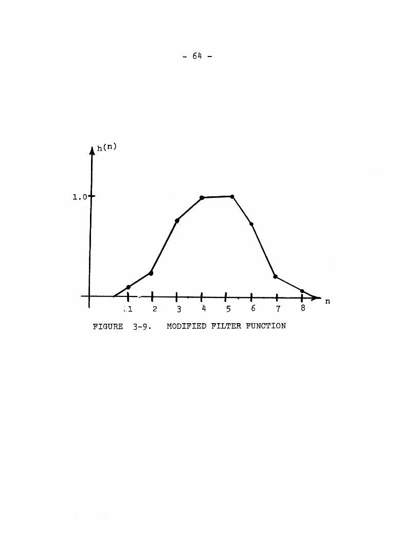
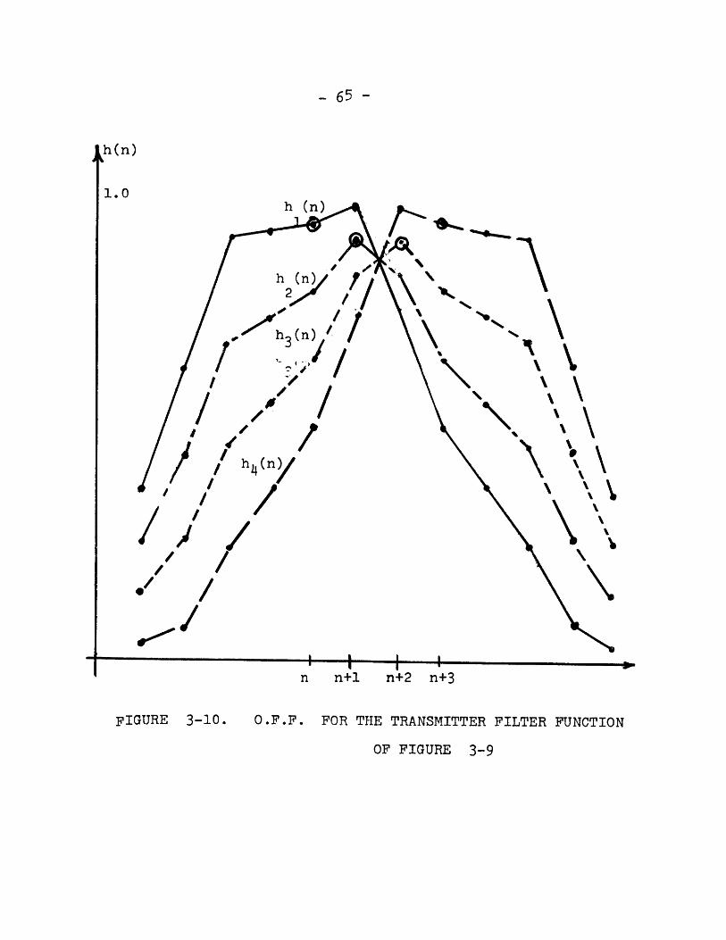
To improve the filter shapes of figure 3-8, the coefficients of

the transmitter triangular filter function may be rechosen as in figure

3-9. This results in a more symmetrical group of modulo filter functions

(figure 3-10). All of the processed test pictures except figure 3-11 use

the overall filter function of figure 3-10. The artifacts introduced by

highly asymmetric overall filter functions are worse for less well-

behaved functions than the monotonic test separations.

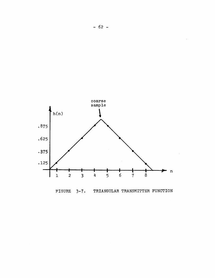
- 62 -

coarsesample

h(n)

n

FIGURE 3-7. TRIANGULAR TRANSMITTER FUNCTION

.875

.625

.375

.125

1 2 3 4 5 6 7 8

- 63 -

\4 h(n)

h/(n)

0000000(n)

h 2 (n)

n n+1 n+2 n+3

FIGURE 3-8. O.F.F. FOR THE TRANSMITTER FILTER FUNCTION

OF FIGURE 3-7

- 64 -

1 2 3 4 5 6 7 8

MODIFIED FILTER FUNCTION

h(n)

1.0

n

FIGURE 3-9.

- 65 -

h(n)

1.0

/+

TV

h (n)

/"pf 4/ h(n/

/1/// /

/

N.

\N

\

n I I In n+1 n+2 n+3

FIGURE 3-10. O.F.F. FOR THE TRANSMITTER FILTER FUNCTION

OF FIGURE 3-9

I

RED BLUE

GREEN

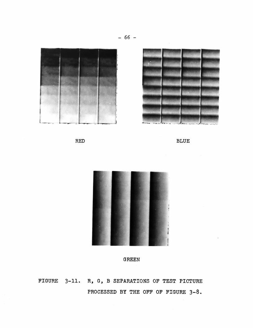
FIGURE 3-11. R, G, B SEPARATIONS OF TEST PICTURE

PROCESSED BY THE OFF OF FIGURE 3-8.

- 67 -

When C 1 and C 2 are processed by the overall filter function and then

inverse transformed with the full resolution luminance to yield the

output red, green, and blue CIE color coordinates at some particular

luminance level, the weighted overall filter averages of C1 and C2 may

yield an illegal triad of R,G,B values necessitating clipping of the R, G,

or B at zero or unity. These illegal codeword artifacts will be more

pronounced with an overall filter function which is highly asymmetric.

Such artifacts are obvious in the processed test picture (figures 2-12

and 2-13) where the green component suddenly changes from its maximum to

minimum values.

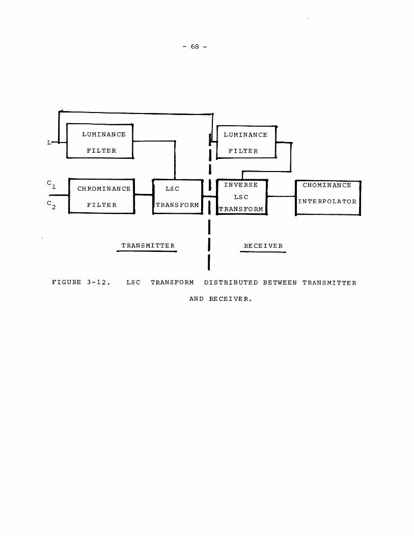
3.3 Luminance Filtering for the LSC Transform

An important issue arises in deciding what value of L should be used

in the LSC transform of Section 2-4, which follows the filter and is the

last operation on the chromaticity components before transmission. To

avoid decoding illegal values of C and C 2, L should strictly be chosen

as the minimum L among all of the pels contributing to the overall

filter function. This, however, would not permit the full power of the

LSC transform to be realized. Instead, the luminance should be filtered

and coarsely sampled in an identical manner as the chrominance. However,

there is no need to perform the additional operations of interpolation

resulting in a wider overall filter function, since the LSC transform and

its inverse are performed on the chromaticity components before inter-

polation (figure 3-12)

A more conservative bound on the the filtered luminance results from

filtering its logarithmic function. The filtered logarithmic function

will of course have to be exponentiated before LSC transforming. Filtering

- 68 -

TRANSMITTER

III

RECEIVER

FIGURE 3-12. LSC TRANSFORM DISTRIBUTED BETWEEN TRANSMITTER

AND RECEIVER.

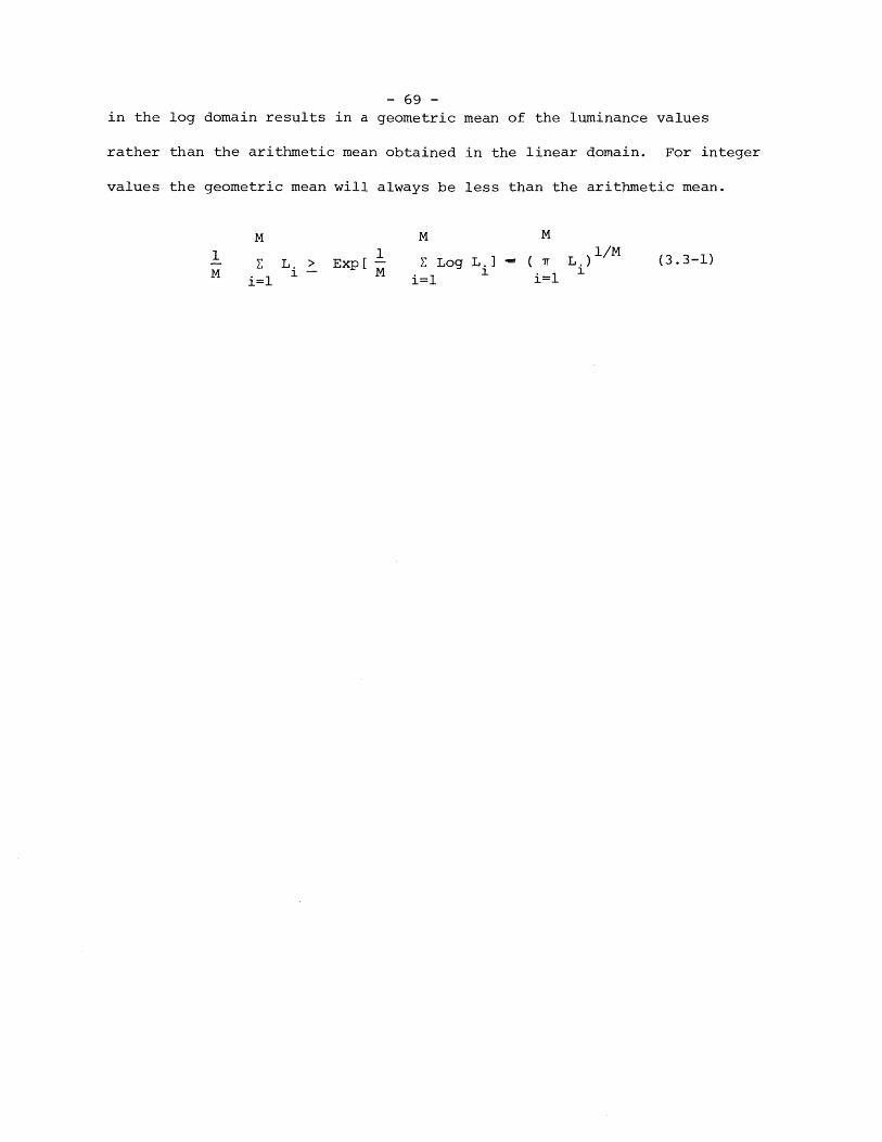
- 69 -in the log domain results in a geometric mean of the luminance values

rather than the arithmetic mean obtained in the linear domain. For integer

values the geometric mean will always be less than the arithmetic mean.

M M M1 1 _l/M

- Z L. > Exp[ - E Log L - ( Tr L.) (3.3-1)M l 1- M 1 i.l 1

- 70 -

IV. Colorimetric Measurement and Photographic Reproduction Approximations

4.1: The Color Photographic Process

4.2: Quasi-Tristimulus Color Measurement

4.3: Colorimetrically Accurate Photographic Reproduction

- 71 -

4.1 The Color Photographic Process

In the previous two chapters, various color coding techniques have

been developed to process psychophysical variables. Therefore, it is

assumed that the color measurements at each pel of the scanned input

picture constitute a proper tristimulus set. Thus for practical color

head filters, transforms must be developed to approximate the tristimulus

functions. This chapter also examines the problem of reproducing the

processed psychophysical parameters of the original print at each pel.

Due to spatial filtering and interpolation of the processed picture,

there may not be a strict colorimetric equivalence between the input

and output picture at each pel, but over fine detail regions the

average color values over an area of several pels should closely match.

The photographic subtractive dye process is the major limitation to

obtaining perfect color reproduction.

In most commercial applications of color facsimile, the red,

green, and blue separations are used to make cyan, magenta, and yellow

press plates for reproduction by printing inks. To avoid the expense

and delay of obtaining color press proofs, it was decided to reproduce

the various test picture separations by photographic techniques. The

photographic continuous tone process is somewhat simpler to analyze

(33)than the printing process since no half tone screen is required,

and the dyes are restricted to overlapping dye layers as contrasted

with individually printed colored inks. However, both processes are

similar in that they use subtractive dyes to synthesize colors. The

entire body of colorimetry, however, has been developed in terms of

additive color reproduction and so the analysis of a subtractive dye

system is rather complex. (34,35)

- 72 -The cyan, magenta, and yellow subtractive dyes reproduce colors

by respectively modulating the transmission of the red, green, and blue

components of the light through the layered dyes. In a reflectance

print, the illuminating light passes through the dyes twice since it

is reflected from the white substrate. Thus, the effective dye density

for reflectance prints is twice the actual density of the dye. An

ideal set of dyes would only absorb light in block bands. For an

equi-energy white illuminant, the reflected light spectrum can be

expressed as a function of the dye spectral density.

p (g) = 10 (4.1-1)

In general, the color coordinate X. of a dye is related to theJ

density by a much more complex relation than a simple exponential

function.

X. = f x.() p(X) dX = f x.(c) 10 dA (4.1-2)J J J

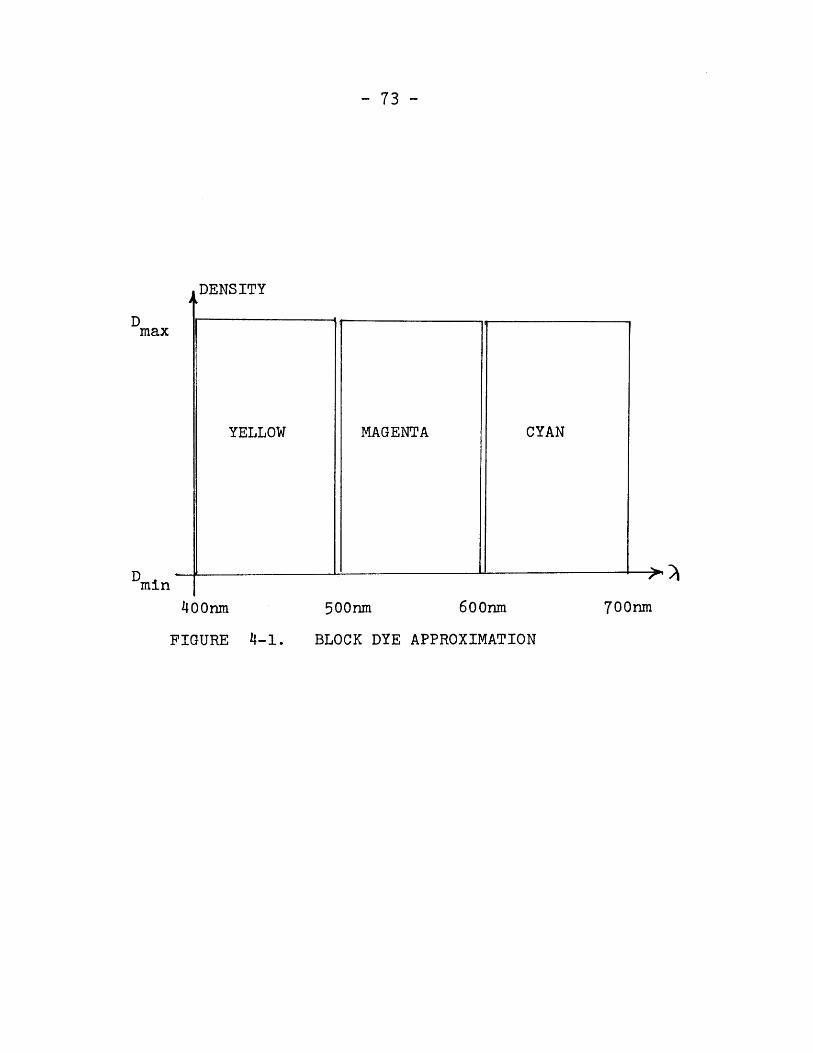
In a block dye approximation (i.e., as in figure 4-1 the cyan dye

absorption is assumed constant over the red band), the spectrally

integrated value of the red component is a simple function of the

cyan density:

-c -cD ( = c R =f r 1 0 dX = c 10 (4.1-3)c Xr

In fact, the cyan dye has unwanted absorptions in the green and blue

range of wavelengths, resulting in a darkening and desaturation of the

- 73 -

DENSITY

Dmax

YELLOW MAGENTA CYAN

Dmin

400nm 500nm 600nn 700nm

BLOCK DYE APPROXIMATIONFIGURE 4-1.

-74-dye. The magenta dye is the least perfect dye, having substantial

absorptions in the red and blue regions of the spectrum. The yellow

dye is the most ideal (figure 4-4).

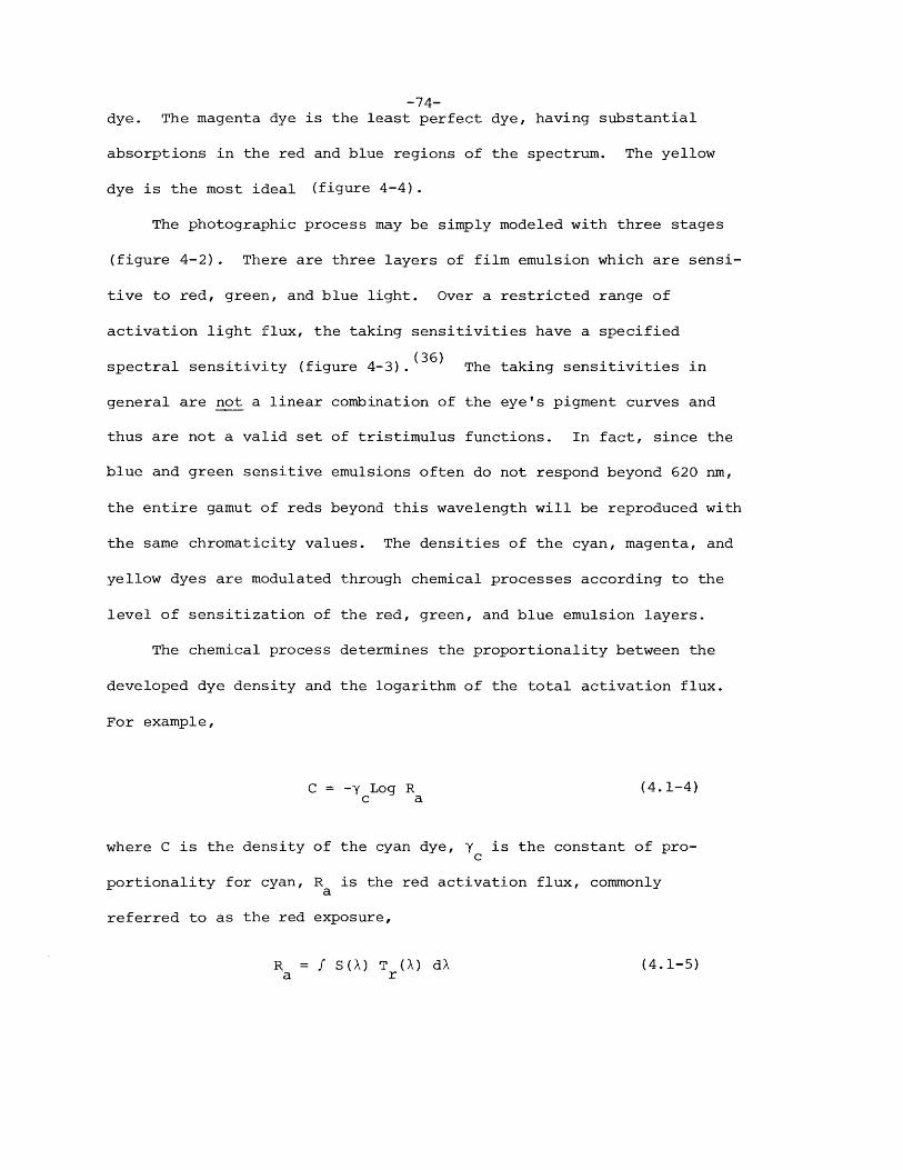
The photographic process may be simply modeled with three stages

(figure 4-2). There are three layers of film emulsion which are sensi-

tive to red, green, and blue light. Over a restricted range of

activation light flux, the taking sensitivities have a specified

spectral sensitivity (figure 4-3).(36) The taking sensitivities in

general are not a linear combination of the eye's pigment curves and

thus are not a valid set of tristimulus functions. In fact, since the

blue and green sensitive emulsions often do not respond beyond 620 nm,

the entire gamut of reds beyond this wavelength will be reproduced with

the same chromaticity values. The densities of the cyan, magenta, and

yellow dyes are modulated through chemical processes according to the

level of sensitization of the red, green, and blue emulsion layers.

The chemical process determines the proportionality between the

developed dye density and the logarithm of the total activation flux.

For example,

C = -Y Log R (4.1-4)c a

where C is the density of the cyan dye, yc is the constant of pro-

portionality for cyan, Ra is the red activation flux, commonly

referred to as the red exposure,

R = f S(A) T (X) dX (4.1-5)a r

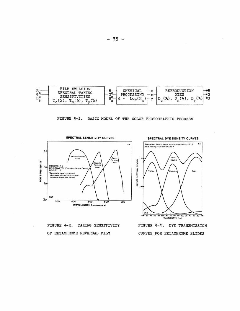
- 75 -

FILM EMULSIONSPECTRAL TAKING

SENSITIVITIESTc(X), Tm("',, Ty('A)

-R CHEMICAL c REPRODUCTION -*RGa- PROCESSING m DYES -GB4 d- Log(H ) -y- D ('A), D (X), D ( BA)-

a a c m y

FIGURE 4-2. BASIC MODEL OF THE COLOR PHOTOGRAPHIC PROCESS

SPECTRAL SENSITIVITY CURVES

I.)

WAVELENGTH (nanometers)

SPECTRAL DYE DENSITY CURVES

Normalized dyes to form a visual neutral density of 1.0 Efor a viewing illuminant of 3200 K

WAVELENGTH (nm)

FIGURE 4-3. TAKING SENSITIVITY

OF EKTACHROME REVERSAL FILM

FIGURE 4-4. DYE TRANSMISSION

CURVES FOR EKTACHROME SLIDES

RGS-BS

S

U)

0

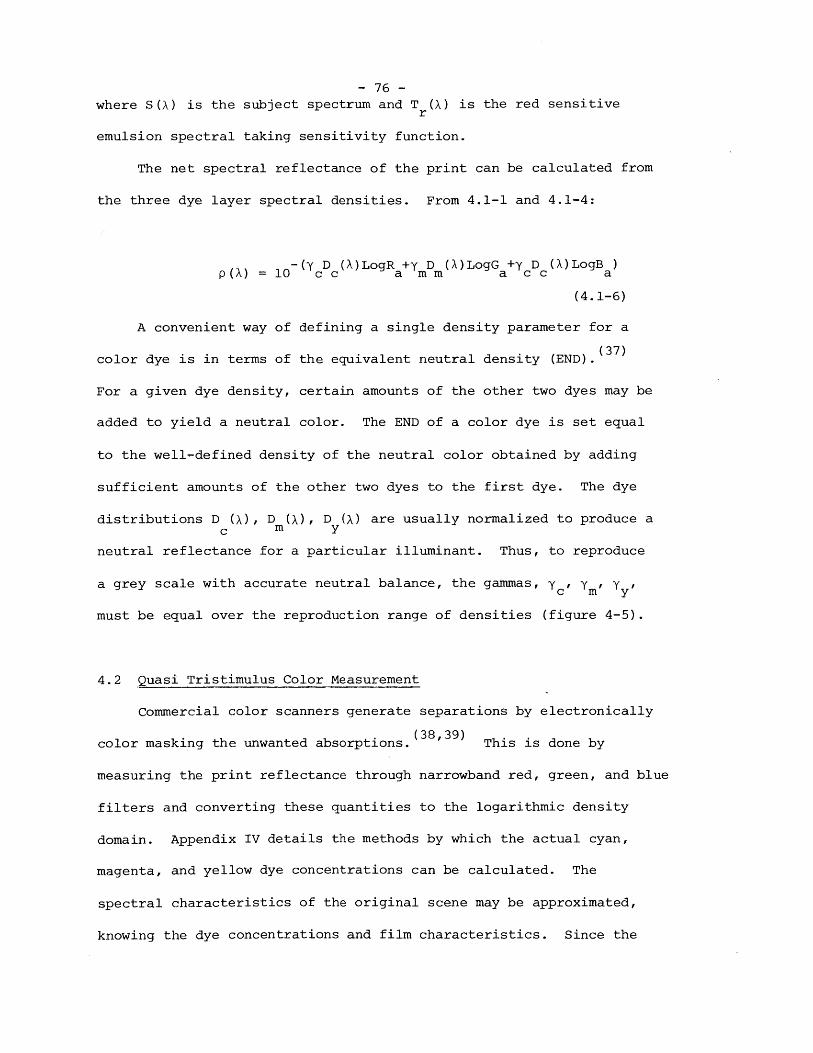
- 76 -where S(X) is the subject spectrum and Tr (X) is the red sensitive

emulsion spectral taking sensitivity function.

The net spectral reflectance of the print can be calculated from

the three dye layer spectral densities. From 4.1-1 and 4.1-4:

-(y D (X)LogR +y D (X)LogG +y D (X)LogB )p(X)=l10 c c a m m a c c a

(4.1-6)

A convenient way of defining a single density parameter for a

color dye is in terms of the equivalent neutral density (END).(3 7 )

For a given dye density, certain amounts of the other two dyes may be

added to yield a neutral color. The END of a color dye is set equal

to the well-defined density of the neutral color obtained by adding

sufficient amounts of the other two dyes to the first dye. The dye

distributions D (X), D (X), D (A) are usually normalized to produce ac m y

neutral reflectance for a particular illuminant. Thus, to reproduce

a grey scale with accurate neutral balance, the gammas, y c' m' y'

must be equal over the reproduction range of densities (figure 4-5).

4.2 Quasi Tristimulus Color Measurement

Commercial color scanners generate separations by electronically

color masking the unwanted absorptions.(38,39) This is done by

measuring the print reflectance through narrowband red, green, and blue

filters and converting these quantities to the logarithmic density

domain. Appendix IV details the methods by which the actual cyan,

magenta, and yellow dye concentrations can be calculated. The

spectral characteristics of the original scene may be approximated,

knowing the dye concentrations and film characteristics. Since the

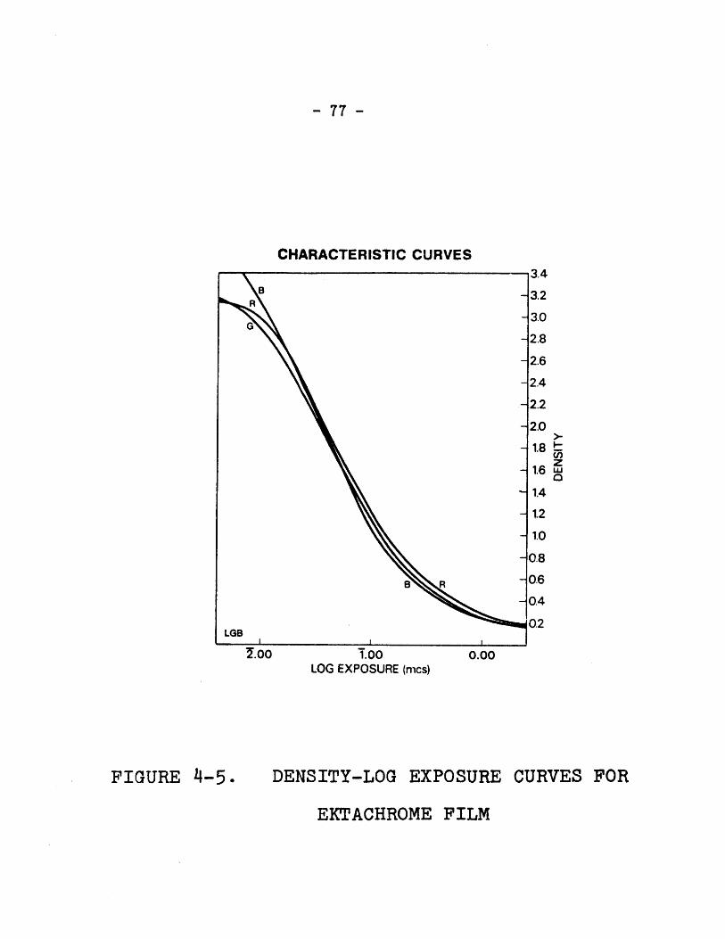
- 77 -

CHARACTERISTIC CURVES

.oo Too 0.00LOG EXPOSURE (ncs)

FIGURE DENSITY-LOG EXPOSURE CURVES

EKTACHROME FILM

zwua

FOR

- 78 -

taking sensitivities are not a proper set of tristimulus curves, the

metamerism of two colors in an original scene may be destroyed. Also,

since the spectral dye density functions are not constant over three

color bands (e.g., 400-500 nm, 500-600 nm, 600-700 nm), the shape of

the reflectance function will not be constant as the density varies.

In color facsimile, the exact colors in the original scene are

usually of little importance. The photograph to be transmitted is

assumed to be of good quality as judged by a photo editor or other

qualified specialist. It is this original photograph which must be

regarded as the subject to be accurately reproduced. A typical sub-

jective evaluation of the effectiveness of the color coder is to compare

the original and processed pictures side by side. Thus the reflectance

measurement of the original scanned print must "see" the print as an

observer's eye.would (i.e., the R,G,B measurement functions should be

a proper set of tristimulus functions).

As an aside, it should be noted that the aforementioned color

masking technique can be used to exactly determine the color coordinates

at each pel. Once the dye concentrations are known, the reflectance

spectral function may be calculated from equation 4.1-6. The

color coordinates may then be found by multiplying this reflectance by

the tristimulus color matching functions and integrating over wavelength.

Such a calculation, however, is far too lengthy to perform at each pel.

A simple method for making valid color measurements at each pel

is to use a proper tristimulus set of detector spectral response

functions. Since these functions are everywhere positive, one or more

of them must have two peaks (from figure 2-1). Filters which closely

approximate a tristimulus set are rather costly. Chapter Five describes

- 79 -

a very economical color head in which the filter functions are primarily

determined by Wratten filters (figure 4-6). A comparison of figures 4-6

and 2-1 shows that the color head response functions least accurately

approximate the tristimulus functions where the red and green responses

overlap. The problem of approximating the CIE R,G,B coordinates from

the color head RH, GH, BH measurements is the topic of this section.

One solution is to linearly transform the color head coordinates.

R RH

=T G H (4.2-1)

B BH

For a one-to-one mapping of the luminance axis, the R = G = B = 1H H H

point must map into the R = G = B = 1 point. Thus, only six independent

coefficients are available for exactly determining the CIE color co-

ordinates for two color points.

Another approach is to separately determine linear transforms of

the color head response functions which approximate the luminance and

chromaticity coordinates. Such a quasi-luminance function will be

correct at all achromatic points if the luminosity coefficients sum to

unity. This follows since RH, GH, and BH are set equal to one for

maximum white, and equation 2.2-3 is therefore valid.

Thus the luminance for the frequently occurring desaturated

colors will be closely approximated by the quasi-luminance function.

The coefficients may be derived to fit the 1931 luminous efficiency

function y( (with the 1951 Judd correction) of figure 2-2, with

minimum mean square error.

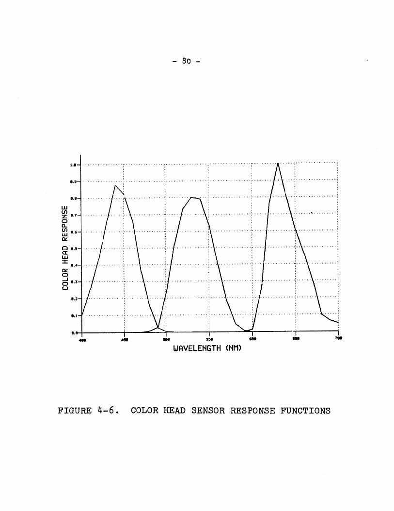
- 80 -

450 56 55.

WAVELENGTH (NM)

COLOR HEAD SENSOR RESPONSE FUNCTIONS

Li

CD7.0(-Low

wO:

-J0

sm

................

................

.. ................

....... .. . . . . . . . . . . . .

. . . . . . . . . . . . . . . . . . . .

. . . . . . . . . . . . . . . . . . . . .

. . . . . . . . . . .

. . . . . . . . . . . . . . . . . . . . .

. . . . . . . . . . . . . . .

. . . . . . . . . . . . . .

. . . . . . . . . . . . . . . . . . . . . . . . . . . . . . . . . . . . . . . . . . . . . . . . . . . . . . . . . . . . . . . . . . . . . . . . . . .

. . . . . . . . . . . . . . . . . . . . . . . . . . . . . . . . . . . . . . . . . . . . . . . . . . . . . . . . . . . . . . . . . . . . . . . . .

. . . . . . . . . . . . . . .. . . . . . . . . . . . . . . . . . . . . . . . . . . . . .. . .

.......... ...... ................ . . . . . . . . . . . . . . . . . . . . . . . . . . .. . . .. . . . . . . . .

. . . . . . .. . .. . . . .. . . . .. . . . . . . . .. . . . . . . . . . . . . . . . . . . . . . . . . . . . . . .7 . . . . . . .

. . . . . . . . .. . . . . . . . . .. . . . . . . . .. . . . . . .. . . . . . . . .

. . . . . . . . . . . . . . .. . . . . . . . . .. . . . . . . . . . . .. . . . . . . . . . . . . . . . . . . . . . . . . . .

. . . . . . . . . . . . . . .. . . . . . . . . . .. . . . . . . . . . . . . . . . . . . . . . . . . . . .

. . . . . . . . . . .. . . . .. .. . . . . . . . . . .. . . . . . . . . . . . . . . . . . . . . . .. . . . .. . . . . . . .

. .. . . . . . . . . . . . . . . . . .. . . . . . . . . . . . . . . . . . . . . . . . . . . . . . . . . . . . . . . . . .

-

FIGURE 4-6.

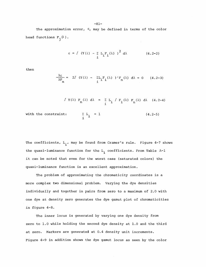
-81-

The approximation error, E, may be defined in terms of the color

head functions F. (X).J

2E = f (Y(A) - E L.F.(X) ) dA (4.2-2)

then

= 2f (Y(A) - EL.F.(X) )'F (A) dA = 0 (4.2-3)F 1 nn

f Y(A) F (A) dA = Z L. i F. (A) F (A) dA (4.2-4)n .i n

with the constraint: = 1 (4.2-5)1

The coefficients, L., may be found from Cramer's rule. Figure 4-7 shows

the quasi-luminance function for the L. coefficients. From Table A-1

it can be noted that even for the worst case (saturated colors) the

quasi-luminance function is an excellent approximation.

The problem of approximating the chromaticity coordinates is a

more complex two dimensional problem. Varying the dye densities

individually and together in pairs from zero to a maximum of 2.0 with

one dye at density zero generates the dye gamut plot of chromaticities

in figure 4-8.

The inner locus is generated by varying one dye density from

zero to 1.0 while holding the second dye density at 1.0 and the third

at zero. Markers are generated at 0.4 density unit increments.

Figure 4-9 in addition shows the dye gamut locus as seen by the color

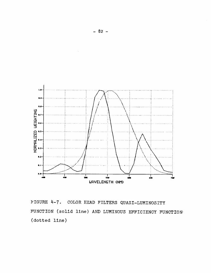
- 82 -

z

w

w

0z

.... ......... ..... ........... : ... .............

. . . . .. . . . . . . . . . . . . . . . . . . . . . . . . . . . . . . . . . . . . . .

7 . . .. . .. . . . .. . . .. . .. . . .. . . . .. . . . .

..........

. . .. . . . .. . .. .. . . .. . .. . . . .. . .. . . .. . . . .. . . . ..

.. . . .. . . .. .7 . . .. . . .. . .. . . .. . .. . . . .. . . . ..

. . . . .. . .. . . .. . . . . . . .. . . . . ... . .. . .. . . . .. . .

. . . . .. . .. . . .. . . .. . . . .. . . . . . .. . . .. . . . . .. . .

. . . .. . .. . . . . . . . . . .. . . . . .. . .. . . . . .. . . .

. .. .. .. . .. . . . . .. . . .

. . .. . .. . ..

.. .... .. .... .... .. .... ... ... .... .. ... ... .

.... . . .. . . .. .. . .. . .. . . . .. . .. .. . ..

.. .. . . ... ... .. .. ... . .. .. .... ....

4

. .. . . .. . .. . .. . .. . . .. . .. . .. . . .. .. .

. .. . .. . . .. . .. . .. . .. . . .. . .. . .. . .. .. .. . .. . ..

.. . . .. . .. . . .. . .. . . . .. . .. . .. .. . . .. .. . . .. .

. . . .. . . .. . . . . . .. . .. . ..

. . .. . . .. . . .. . .. .. . . .. . . .. . .. . .. . . . . . .. . .

. . .. . . .. . .. . .. . .. . . .. . .. . . .. .

. .. . . . .. . .

4.. 4. S.. 3. ... C.. ,.0

WAVELENGTH (NM)

FIGURE 4-7. COLOR HEAD FILTERS QUASI-LUMINOSITY

FUNCTION (solid line) AND LUMINOUS EFFICIENCY FUNCTION,

(dotted line)

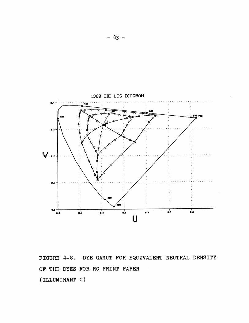
- 83 -

1960 CIE-UCS DIAGRAM

U

FIGURE 4-8. DYE GAMUT FOR EQUIVALENT NEUTRAL DENSITY

OF THE DYES FOR RC PRINT PAPER

(ILLUMINANT C)

V

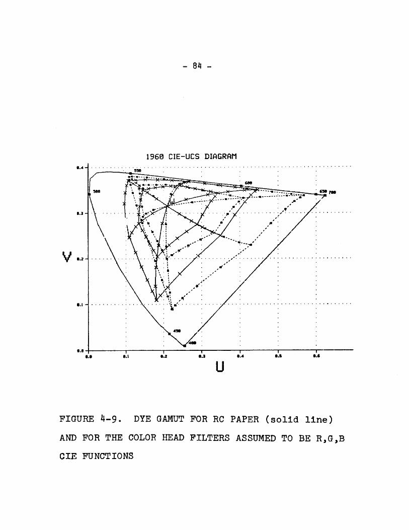
- 84 -

1960 CIE-UCS DIAGRAM6.4__* - 5

U

4-9. DYE GAMUT FOR RC PAPER (solid line)

AND FOR THE COLOR HEAD FILTERS ASSUMED TO BE R,G,B

CIE FUNCTIONS

8.3-

V .2

.1

e.g

FIGURE

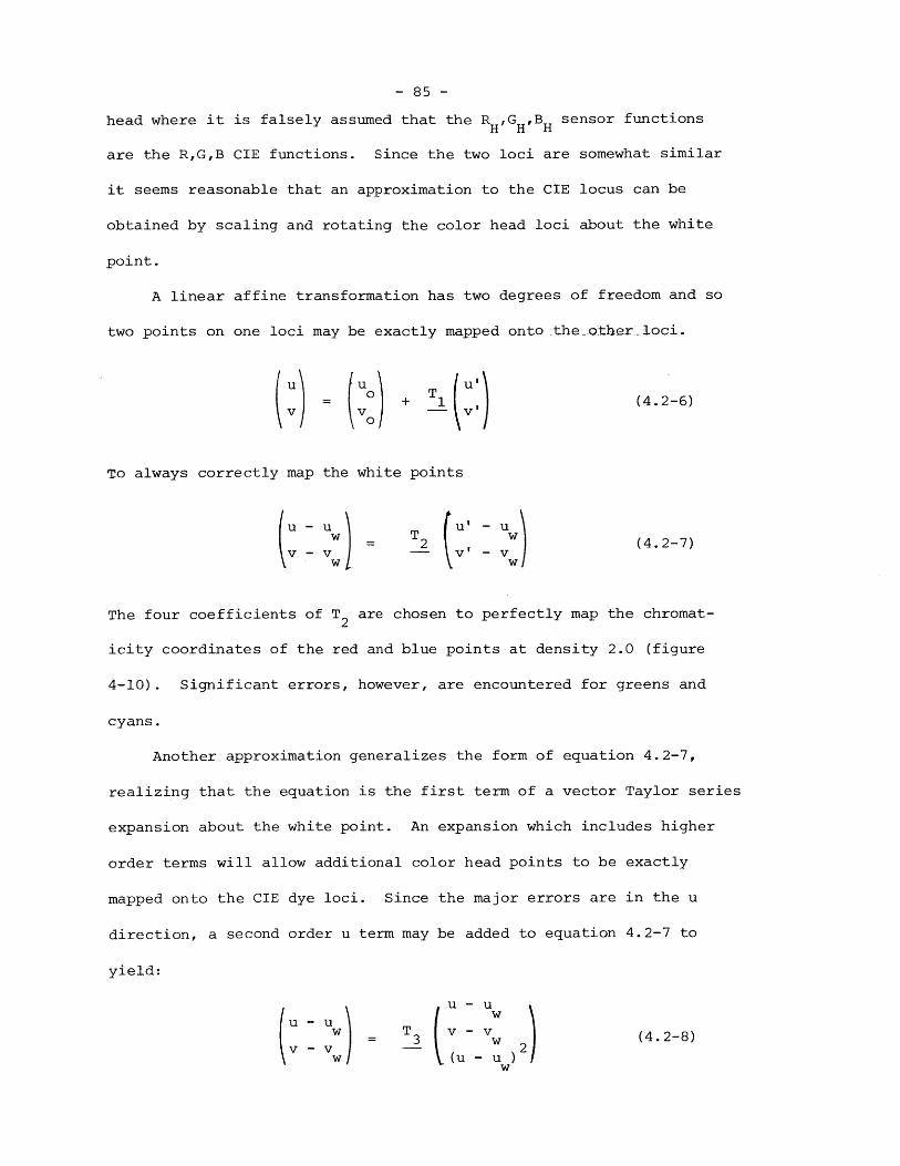
- 85 -

head where it is falsely assumed that the R H,G H,BH sensor functions

are the R,G,B CIE functions. Since the two loci are somewhat similar

it seems reasonable that an approximation to the CIE locus can be

obtained by scaling and rotating the color head loci about the white

point.

A linear affine transformation has two degrees of freedom and so

two points on one loci may be exactly mapped onto the -other loci.

( = 0 + 1 (4.2-6)v v -- v'

To always correctly map the white points

(> w T2 (, u w (4.2-7)v - v -- v1 - v

w w

The four coefficients of T2 are chosen to perfectly map the chromat-

icity coordinates of the red and blue points at density 2.0 (figure

4-10). Significant errors, however, are encountered for greens and

cyans.

Another approximation generalizes the form of equation 4.2-7,

realizing that the equation is the first term of a vector Taylor series

expansion about the white point. An expansion which includes higher

order terms will allow additional color head points to be exactly

mapped onto the CIE dye loci. Since the major errors are in the u

direction, a second order u term may be added to equation 4.2-7 to

yield:

u -uw

w _ T3 v - v (4.2-8)v -v ~ _w 2

w (u -u w)

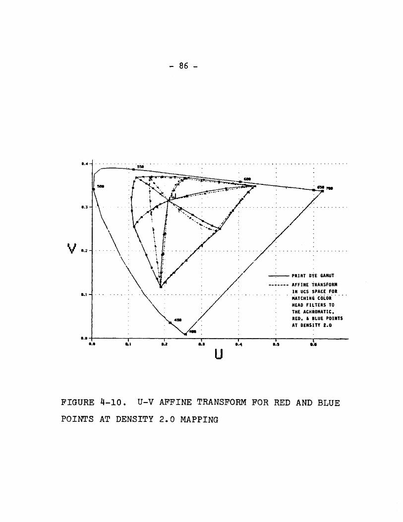
- 86 -

6.3 -T . . . . . . . . . .. -- . . . . . . . . . .. .. . . ..

PRINT DYE GANUT

------- AFFINE TRANSFORNIN UCS SPACE FOR

.................. ...........................MATCHING COLORHEAD FILTERS TO

- .THE ACHRONATIC,

49 RED, & BLUE POINTS- - -- AT DENSITY 2.0

48.4U.S 4.$ 3.2 aLs 5.4 U.S 6.6

U

FIGURE 4-10. U-V AFFINE TRANSFORM FOR RED AND BLUE

POINTS AT DENSITY 2.0 MAPPING

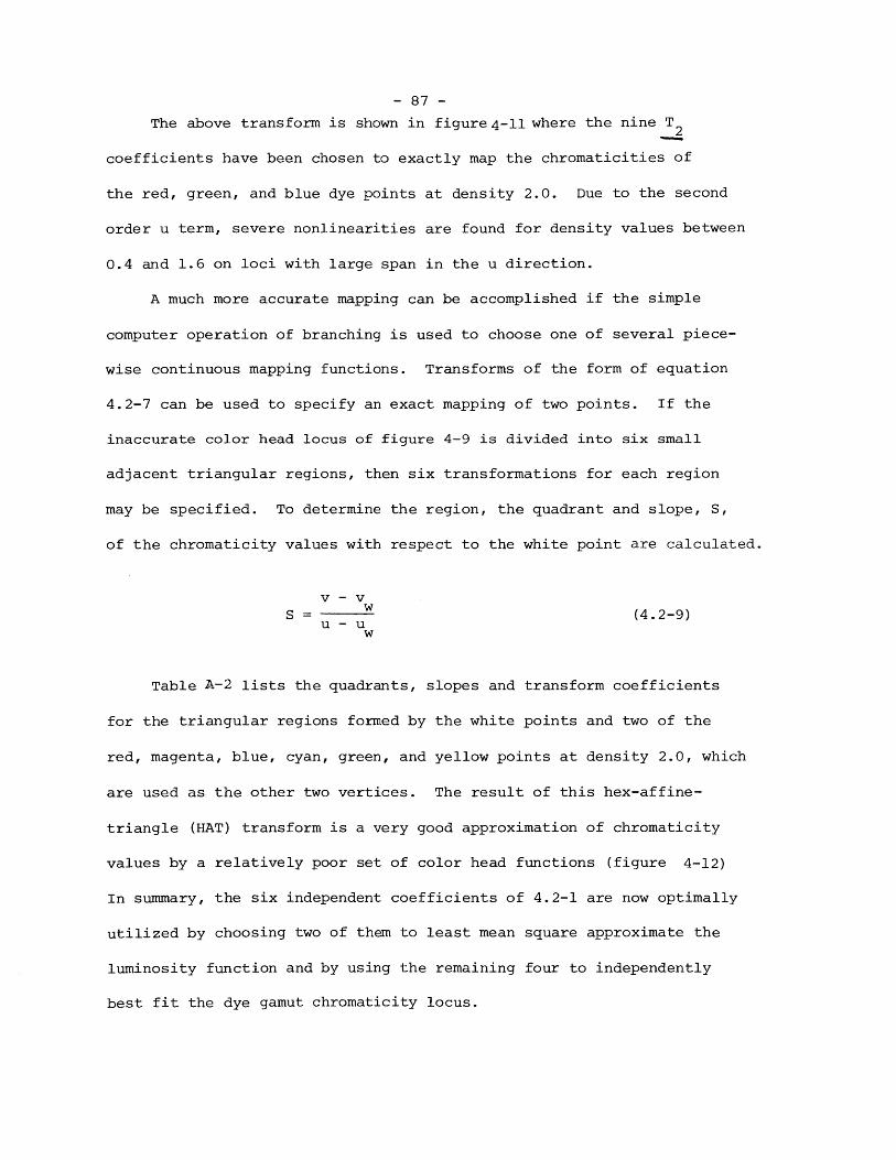
- 87 -

The above transform is shown in figure 4-11 where the nine T

coefficients have been chosen to exactly map the chromaticities of

the red, green, and blue dye points at density 2.0. Due to the second

order u term, severe nonlinearities are found for density values between

0.4 and 1.6 on loci with large span in the u direction.

A much more accurate mapping can be accomplished if the simple

computer operation of branching is used to choose one of several piece-

wise continuous mapping functions. Transforms of the form of equation

4.2-7 can be used to specify an exact mapping of two points. If the

inaccurate color head locus of figure 4-9 is divided into six small

adjacent triangular regions, then six transformations for each region

may be specified. To determine the region, the quadrant and slope, S,

of the chromaticity values with respect to the white point are calculated.

v -vS = (4.2-9)

u -uw

Table A-2 lists the quadrants, slopes and transform coefficients

for the triangular regions formed by the white points and two of the

red, magenta, blue, cyan, green, and yellow points at density 2.0, which

are used as the other two vertices. The result of this hex-affine-

triangle (HAT) transform is a very good approximation of chromaticity

values by a relatively poor set of color head functions (figure 4-12)

In summary, the six independent coefficients of 4.2-1 are now optimally

utilized by choosing two of them to least mean square approximate the

luminosity function and by using the remaining four to independently

best fit the dye gamut chromaticity locus.

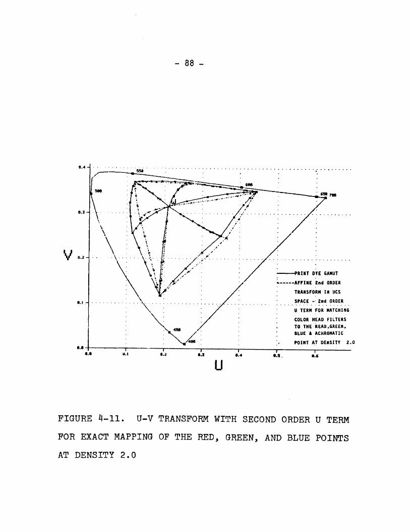
- 88 -

_55a

650 m

PRINT DYE GAMUT

-----AFFINE 2nd ORDER

TRANSFORM IN UCS

. SPACE - 2nd ORDER

U TERM FOR MATCHING

COLOR HEAD FILTERSTO THE READ.GREEN,BLUE & ACHROMATIC

1~.5.

POINT AT DENSITY 2.0

9

U

FIGURE 4-11. U-V

FOR EXACT MAPPING

TRANSFORM WITH SEC

OF THE RED, GREEN,

OND ORDER U TERM

AND BLUE POINTS

AT DENSITY

V 0.2

SI -

U.. -

2.0

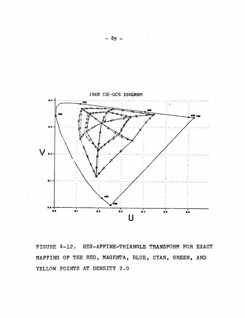
- 89 -

1960 CIE-UCS DIAGRAM

U

FIGURE 4-12. HEX-AFFINE-TRIANGLE TRANSFORM FOR EXACT

MAPPING OF THE RED, MAGENTA, BLUE, CYAN, GREEN,

YELLOW POINTS AT DENSITY

V

AND

2.0

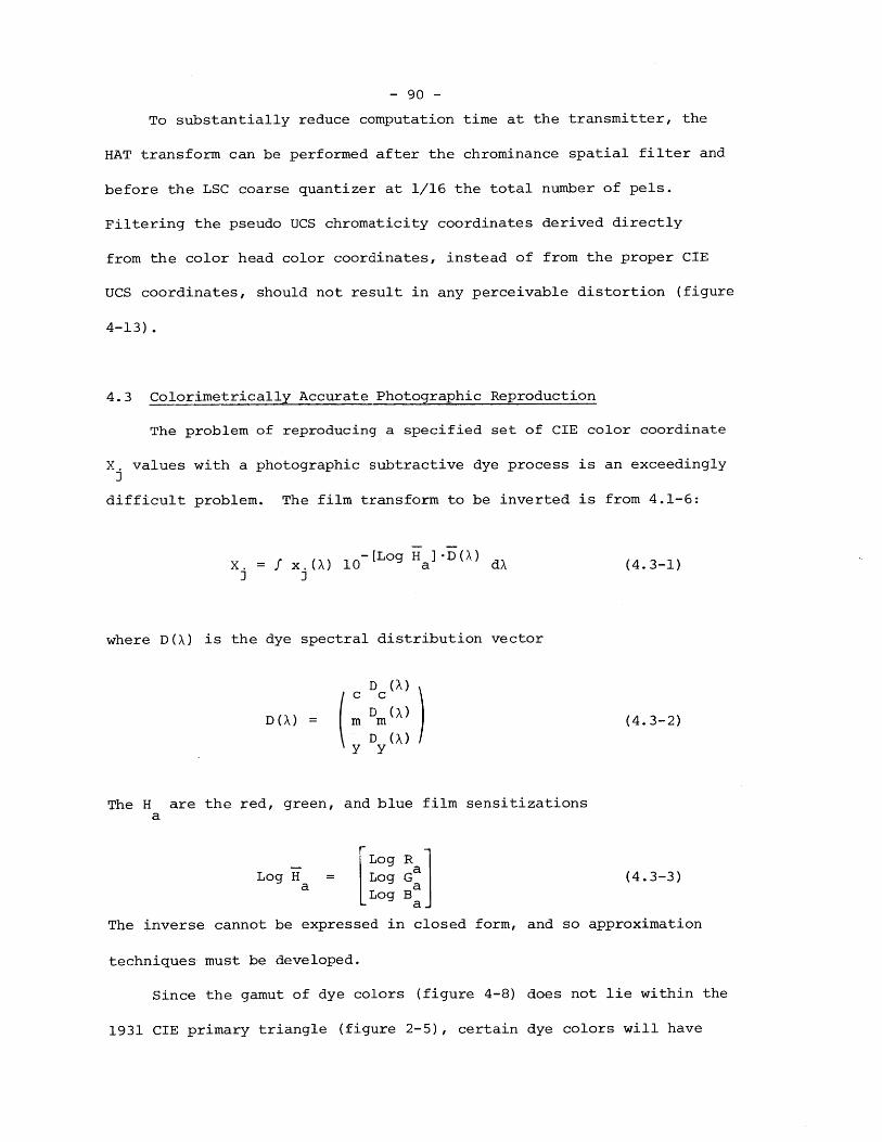
- 90 -

To substantially reduce computation time at the transmitter, the

HAT transform can be performed after the chrominance spatial filter and

before the LSC coarse quantizer at 1/16 the total number of pels.

Filtering the pseudo UCS chromaticity coordinates derived directly

from the color head color coordinates, instead of from the proper CIE

UCS coordinates, should not result in any perceivable distortion (figure

4-13).

4.3 Colorimetrically Accurate Photographic Reproduction

The problem of reproducing a specified set of CIE color coordinate

X. values with a photographic subtractive dye process is an exceedinglyJ

difficult problem. The film transform to be inverted is from 4.1-6:

X. = f x(AX) 1 0 [Log Ha ]-D() dA (4.3-1)J J

where D(X) is the dye spectral distribution vector

D (A)c c

D(X) = m D m (X) (4.3-2)

D (A)y y

The H are the red, green, and blue film sensitizationsa

Log R

Log H Log Ga (4.3-3)

Log B-a.

The inverse cannot be expressed in closed form, and so approximation

techniques must be developed.

Since the gamut of dye colors (figure 4-8) does not lie within the

1931 CIE primary triangle (figure 2-5), certain dye colors will have

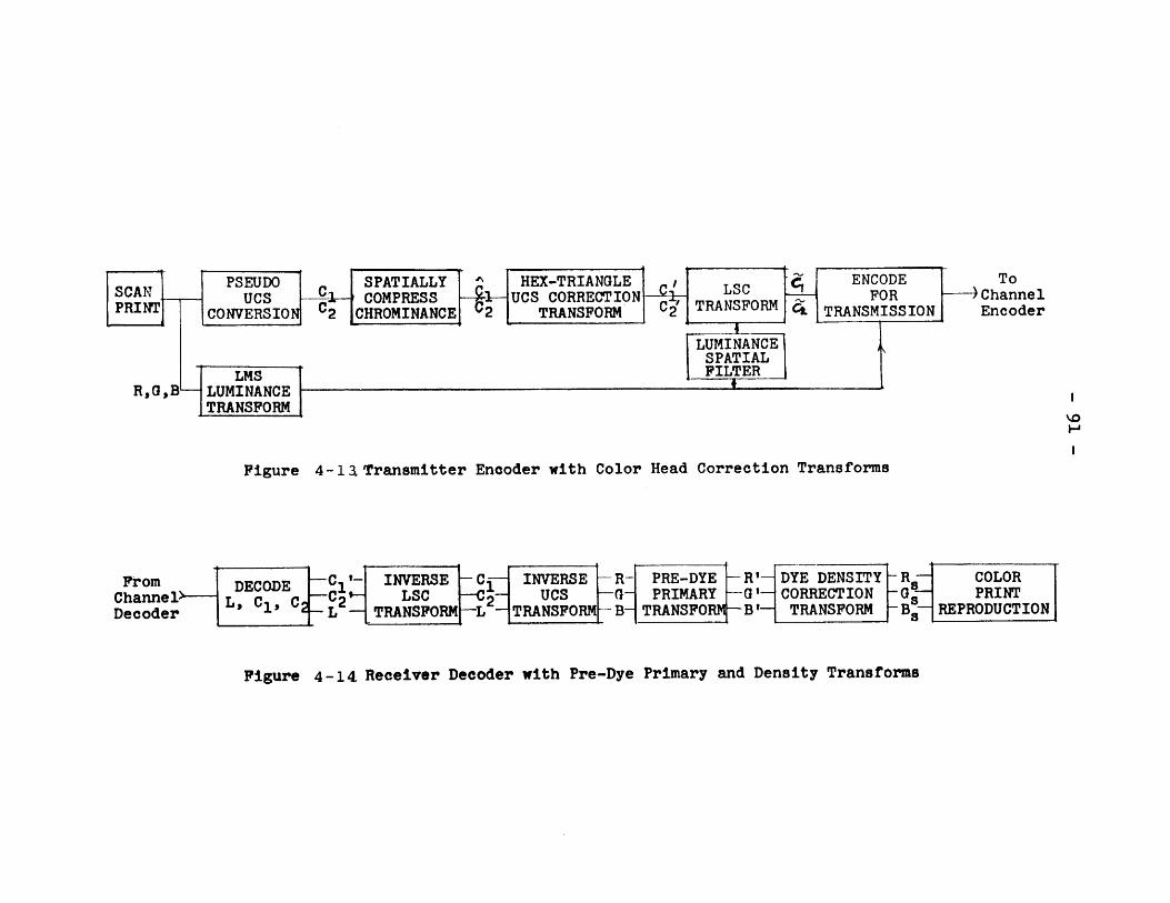
PSEUDO SPATIALLY HEX-TRIANGLE , ENCODE ToSCAN-- UCS C COMPRESS - UCS CORRECT ION LSC R FOR Channel

CONVERSION 2 CHROMINANCE 02 TRANSFORM C2 TRANSFORM t TRANSMISSION Encoder

LUMINANCESPATIAL

LMS FILTER

R,G,B LUMINANCETRANSFORM

Figure 4-1a Transmitter Encoder with Color Head Correction Transforms

From DECODE C 1 '- INVERSE -C INVERSE -R- PRE-DYE -R'- DYE DENSITY -R COLOR

Channel) L C1 , C C2 LSC 2- UCS -0 PRIMARY -G'- CORRECTION -G- PRINT

Decoder * L TRANSFORM - TRANSFORM-B TRANSFORM-B'- TRANSFORM -Bs REPRODUCTION

Figure 4-14 Receiver Decoder with Pre-Dye Primary and Density Transforms

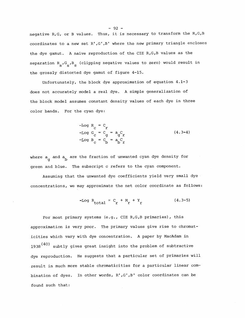
- 92 -

negative R,G, or B values. Thus, it is necessary to transform the R,G,B

coordinates to a new set R',G',B' where the new primary triangle encloses

the dye gamut. A naive reproduction of the CIE R,G,B values as the

separation R ,G ,B (clipping negative values to zero) would result ins s s

the grossly distorted dye gamut of figure 4-15.

Unfortunately, the block dye approximation of equation 4.1-3

does not accurately model a real dye. A simple generalization of

the block model assumes constant density values of each dye in three

color bands. For the cyan dye:

-!hog R = Cc r

-Log G = C = a C (4.3-4)c g g r

-tog B = Cb = abCr

where a and ab are the fraction of unwanted cyan dye density forgb

green and blue. The subscript c refers to the cyan component.

Assuming that the unwanted dye coefficients yield very small dye

concentrations, we may approximate the net color coordinate as follows:

-Log R ~ C + M + Y (4.3-5)total r r r

For most primary systems (e.g., CIE R,G,B primaries), this

approximation is very poor. The primary values give rise to chromat-

icities which vary with dye concentration. A paper by MacAdam in

1938(40) subtly gives great insight into the problem of subtractive

dye reproduction. He suggests that a particular set of primaries will

result in much more stable chromaticities for a particular linear com-

bination of dyes. In other words, R',G',B' color coordinates can be

found such that:

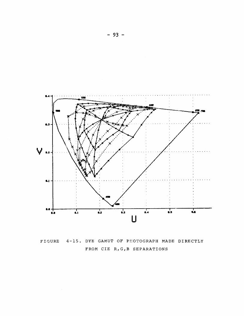
- 93 -

.n .x--...--.........

x x

8 .2 - - . . .-. -.-.-.-.-.-.-.-.-.-.-.-.-.-.-.-.-.-.-.-.-.-

V.2

6.0 8.1 8.2 6. 6.4 6.s

U

FIGURE 4-15. DYE GAMUT OF PHOTOGRAPH MADE DIRECTLY

FROM CIE R,G,B SEPARATIONS

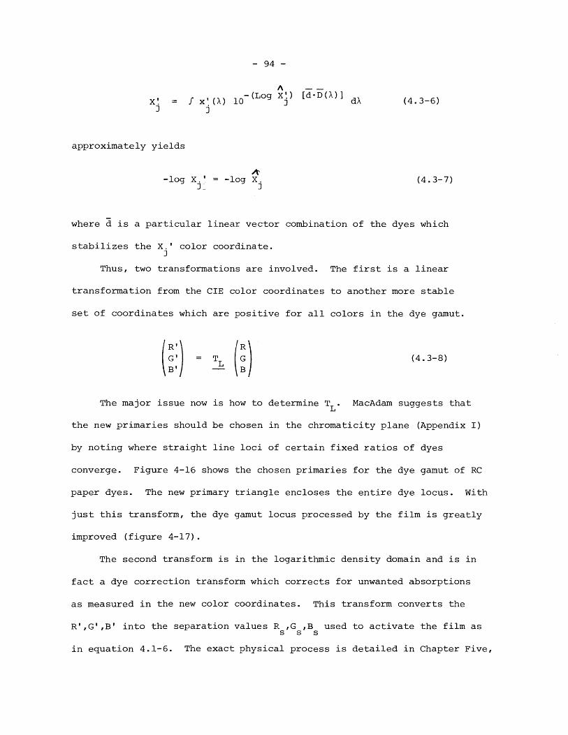
- 94 -

A -

x ( I-(Log X'.) [d-D(X)]X' = f x'(M 10 J dX (4.3-6)J j

approximately yields

-log X.' = -log X. (4.3-7)J J

where d is a particular linear vector combination of the dyes which

stabilizes the X.' color coordinate.J

Thus, two transformations are involved. The first is a linear

transformation from the CIE color coordinates to another more stable

set of coordinates which are positive for all colors in the dye gamut.

R' R

G' = TL G (4.3-8)B' - B

The major issue now is how to determine T . MacAdam suggests that

the new primaries should be chosen in the chromaticity plane (Appendix I)

by noting where straight line loci of certain fixed ratios of dyes

converge. Figure 4-16 shows the chosen primaries for the dye gamut of RC

paper dyes. The new primary triangle encloses the entire dye locus. With

just this transform, the dye gamut locus processed by the film is greatly

improved (figure 4-17).

The second transform is in the logarithmic density domain and is in

fact a dye correction transform which corrects for unwanted absorptions

as measured in the new color coordinates. This transform converts the

R',G',B' into the separation values R ,G ,B used to activate the film ass s s

in equation 4.1-6. The exact physical process is detailed in Chapter Five,

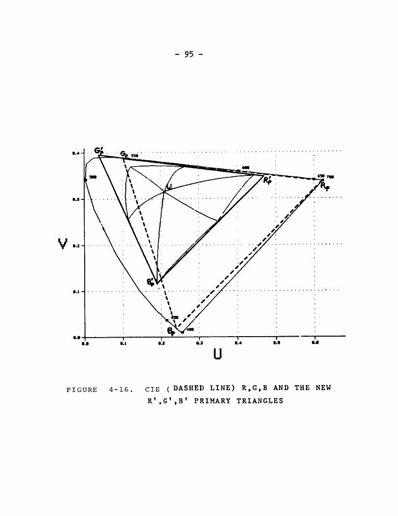
- 95 -

0.2 ............ ...... ...... . ..

3.1

s. - - - - - - - - - -- - --

e.g 6.1 8.2 0.3

FIGURE 4-16. CIE ( DASHED

U

LINE) R,G,B AND THE

R',G',B' PRIMARY TRIANGLES

NEW

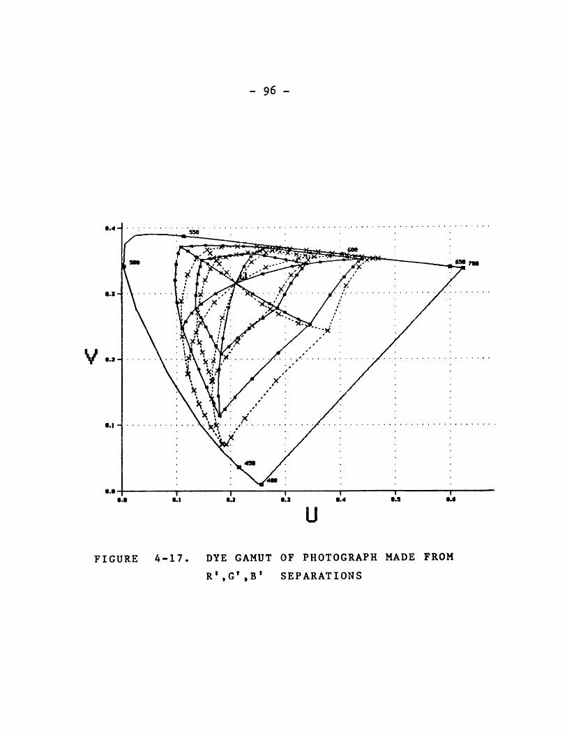
- 96 -

s.4

6.6 - --

v.B

FIGURE

U

4-17. DYE GAMUT

R',G' ,B'

OF PHOTOGRAPH

SEPARATIONS

MADE FROM

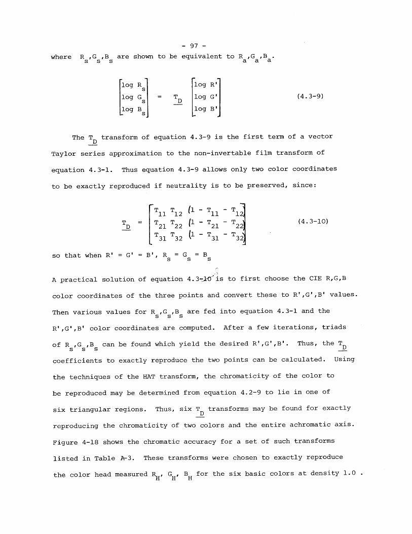
- 97 -

where R ,G ,B are shown to be equivalent to R ,G , B .s s s a a a

log Rs log R'

log G = T log G' (4.3-9)

log B log B'

The T transform of equation 4.3-9 is the first term of a vector-D

Taylor series approximation to the non-invertable film transform of

equation 4.3-1. Thus equation 4.3-9 allows only two color coordinates

to be exactly reproduced if neutrality is to be preserved, since:

T11 12 (1 T11 12

T = T T l T (1 T E'i (4.3-10)

LT31 T32 (1 T31 T32

so that when R' = G' = B', R = G = BS S S

A practical solution of equation 4.3-l-a'is to first choose the CIE R,G,B

color coordinates of the three points and convert these to R',G',B' values.

Then various values for R ,G ,B are fed into equation 4.3-1 and theS S S

R',G',B' color coordinates are computed. After a few iterations, triads

of R ,G ,B can be found which yield the desired R',G',B'. Thus, the T

coefficients to exactly reproduce the two points can be calculated. Using

the techniques of the HAT transform, the chromaticity of the color to

be reproduced may be determined from equation 4.2-9 to lie in one of

six triangular regions. Thus, six TD transforms may be found for exactly

reproducing the chromaticity of two colors and the entire achromatic axis.

Figure 4-18 shows the chromatic accuracy for a set of such transforms

listed in Table A-3. These transforms were chosen to exactly reproduce

the color head measured RH, GH, BH for the six basic colors at density 1.0

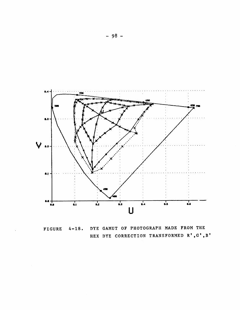
- 98 -

.. . . . . .

FIGURE 4-18.

U

DYE GAMUT OF PHOTOGRAPH MADE FROM THE

HEX DYE CORRECTION TRANSFORMED R',G',B'

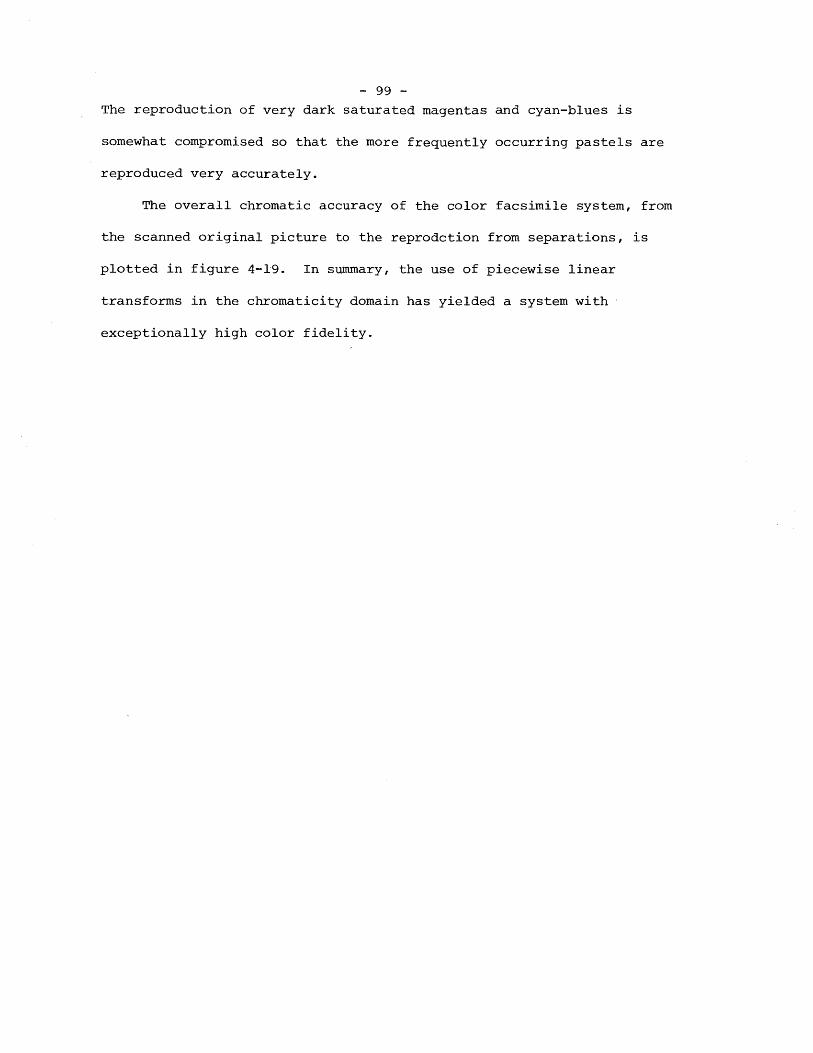
- 99 -

The reproduction of very dark saturated magentas and cyan-blues is

somewhat compromised so that the more frequently occurring pastels are

reproduced very accurately.

The overall chromatic accuracy of the color facsimile system, from

the scanned original picture to the reprodction from separations, is

plotted in figure 4-19. In summary, the use of piecewise linear

transforms in the chromaticity domain has yielded a system with

exceptionally high color fidelity.

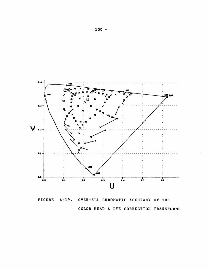
- 100 -

8.4 1__ __ . . . . . . . . . . ..536 .... .. . . ..

mW

x A

x

7..

Kc

I3.3 ... - . - - K- M -- - - -- - ' '

' / . ...... X. .. K......

x IK )d X

6.0 U.S 6.2 6.3 6.4 6.3 6.6

UFIGURE 4-19. OVER-ALL CHROMATIC ACCURACY OF THE

COLOR HEAD & DYE CORRECTION TRANSFORMS

- 101 -

V. Simulation of the Color Facsimile System

5.1 Introduction

5.2 The Color Scanner

5.3 The Computer and Software System

5.4 Reconstruction of Color Pictures

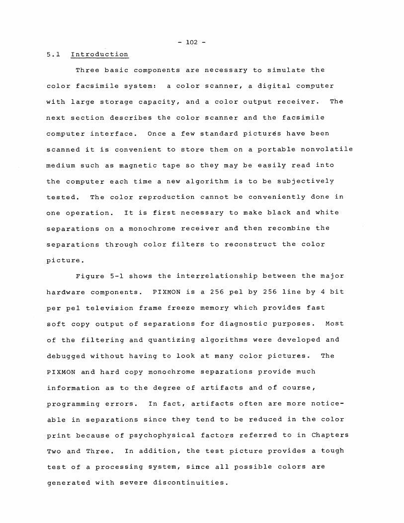
- 102 -

5.1 Introduction

Three basic components are necessary to simulate the

color facsimile system: a color scanner, a digital computer

with large storage capacity, and a color output receiver. The

next section describes the color scanner and the facsimile

computer interface. Once a few standard pictures have been

scanned it is convenient to store them on a portable nonvolatile

medium such as magnetic tape so they may be easily read into

the computer each time a new algorithm is to be subjectively

tested. The color reproduction cannot be conveniently done in

one operation. It is first necessary to make black and white

separations on a monochrome receiver and then recombine the

separations through color filters to reconstruct the color

picture.

Figure 5-1 shows the interrelationship between the major

hardware components. PIXMON is a 256 pel by 256 line by 4 bit

per pel television frame freeze memory which provides fast

soft copy output of separations for diagnostic purposes. Most

of the filtering and quantizing algorithms were developed and

debugged without having to look at many color pictures. The

PIXMON and hard copy monochrome separations provide much

information as to the degree of artifacts and of course,

programming errors. In fact, artifacts often are more notice-

able in separations since they tend to be reduced in the color

print because of psychophysical factors referred to in Chapters

Two and Three. In addition, the test picture provides a tough

test of a processing system, since all possible colors are

generated with severe discontinuities.

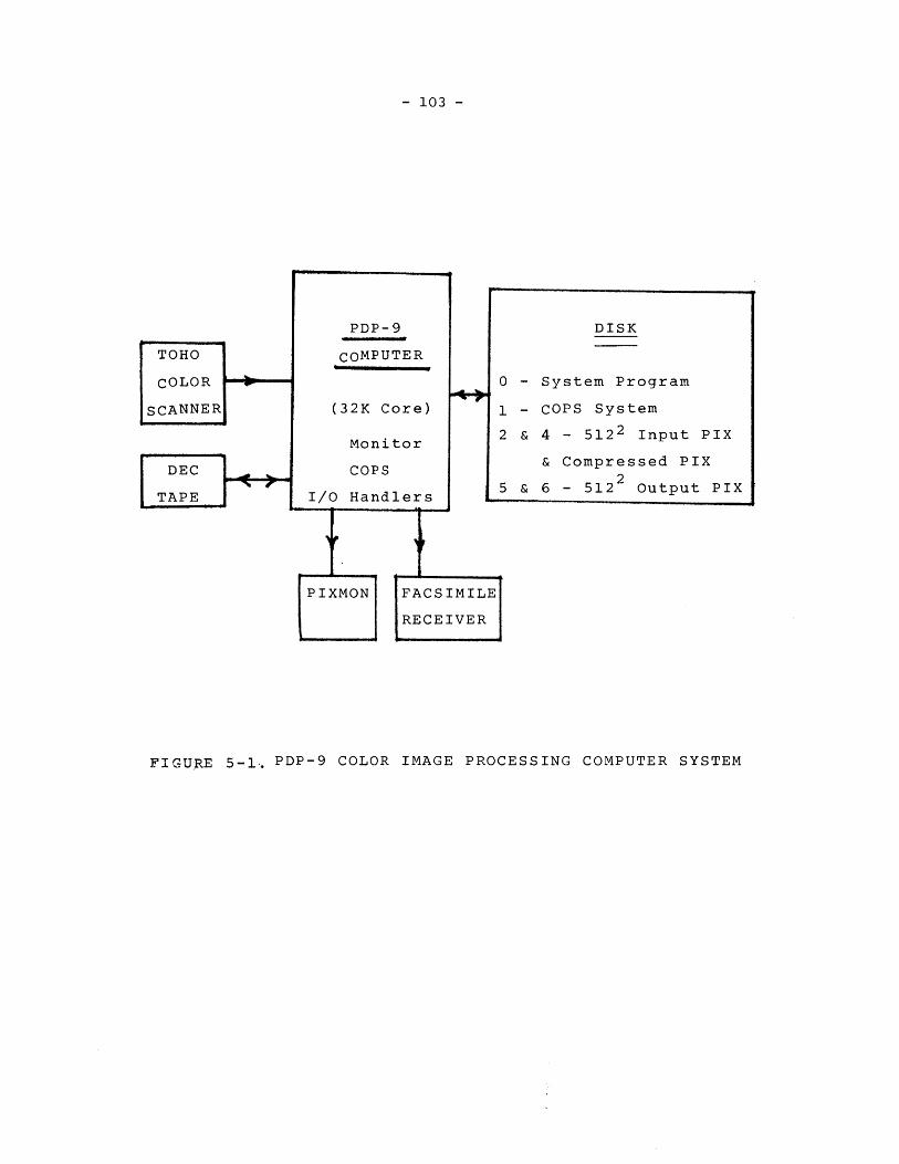
- 103 -

TOHO

COLOR

SCANNER

DEC

TAPE

PIXMON FACSIMILE

RECEIVER

FIGURE 5-1,. PDP-9 COLOR IMAGE PROCESSING COMPUTER SYSTEM

PDP-9

COMPUTER

(32K Core)

Monitor

COPS

I/O Handlers

DISK

0 - System Program

1 - COPS System

2 & 4 - 5122 Input PIX

& Compressed PIX

5 & 6 - 5122 Output PIX

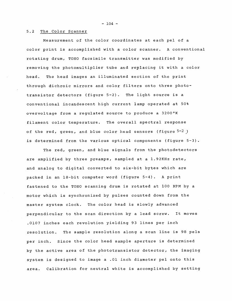
- 104 -

5.2 The Color Scanner

Measurement of the color coordinates at each pel of a

color print is accomplished with a color scanner. A conventional

rotating drum, TOHO facsimile transmitter was modified by

removing the photomultiplier tube and replacing it with a color

head. The head images an illuminated section of the print

through dichroic mirrors and color filters onto three photo-

transistor detectors (figure 5-2). The light source is a

conventional incandescent high current lamp operated at 50%

overvoltage from a regulated source to produce a 3200*K

filament color temperature. The overall spectral response

of the red, green, and blue color head sensors (figure 5-2 )

is determined from the various optical components (figure 5-3).

The red, green, and blue signals from the photodetectors

are amplified by three preamps, sampled at a 1.92KHz rate,

and analog to digital converted to six-bit bytes which are

packed in an 18-bit computer word (figure 5-4). A print

fastened to the TOHO scanning drum is rotated at 100 RPM by a

motor which is synchronized by pulses counted down from the

master system clock. The color head is slowly advanced

perpendicular to the scan direction by a lead screw. It moves

.0107 inches each revolution yielding 93 lines per inch

resolution. The sample resolution along a scan line is 98 pels

per inch. Since the color head sample aperture is determined

by the active area of the phototransistor detector, the imaging

system is designed to image a .01 inch diameter pel onto this

area. Calibration for neutral white is accomplished by setting

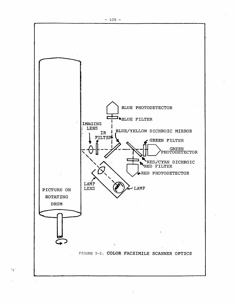
- 105 -

PICTURE ON

ROTATING

DRUM

BLUE PHOTODETECTOR

BLUE FILTERIMAGING

L(NS IR BLUE/YELLOW DICHROIC MIRROR

FILTE GREEN FILTER

..... FJ GREENPHOTODETECTOR

RED/CYAN DICHROICRED FILTER

RED PHOTODETECTOR

LAMPLENS - LAMP

FIGURE 5-2. COLOR FACSIMILE SCANNER OPTICS

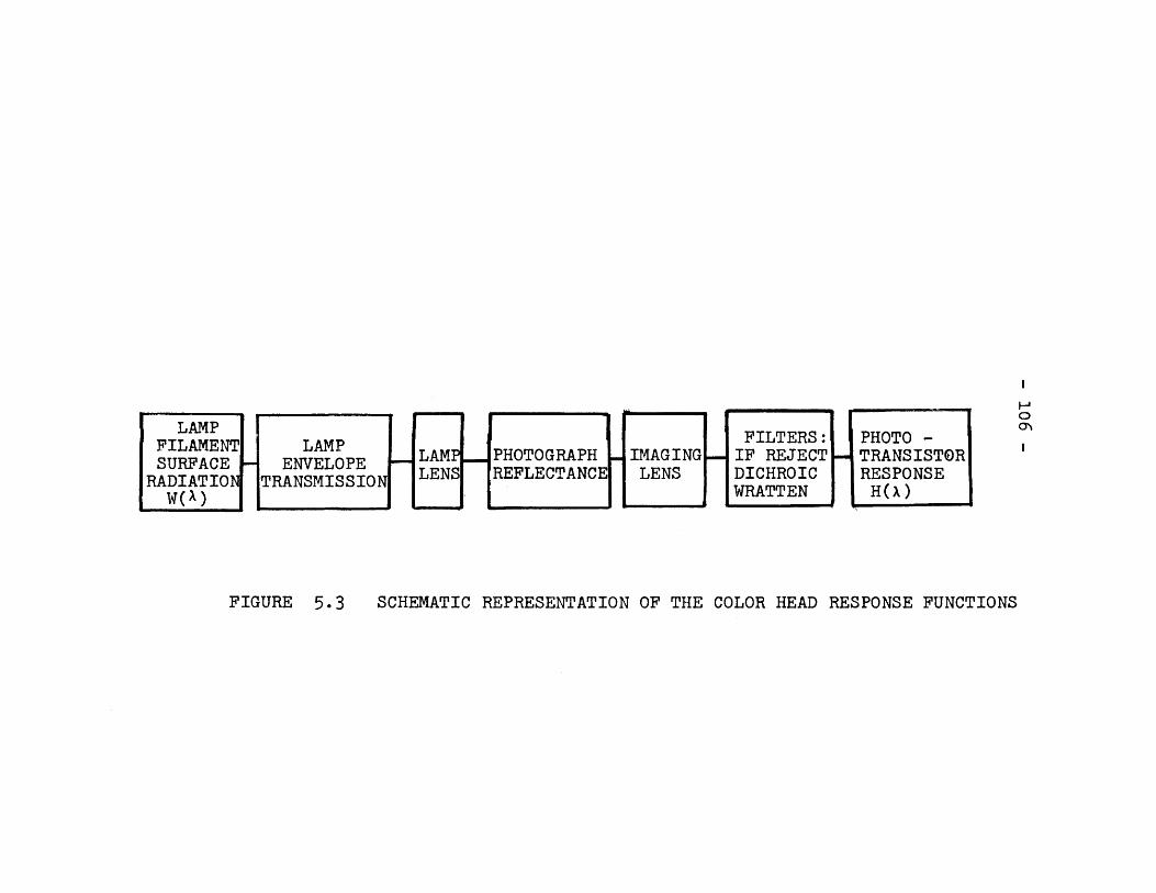
LAMPFILAMENT LAMP FILTERS: PHOTO -

SURFACE ENVELOPE LAM PHOTOGRAPH IMAGING IF REJECT TRANSISTORRADIATIO TRANSMISSION LENS REFLECTANCE LENS DICHROIC RESPONSE

WI) WRATTEN H(X)

FIGURE 5.3 SCHEMATIC REPRESENTATION OF THE COLOR HEAD RESPONSE FUNCTIONS

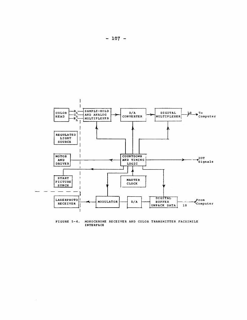
ToComputer

IOTlSignals

rom"Computer

FIGURE 5-4. MONOCHROME RECEIVER AND COLOR TRANSMITTER FACSIMILEINTERFACE

- 107 -

- 108 -

the color head outputs equal to the maximum white level for

the white border of the print.

The picture is initially synchronized by a single start

pulse. Thereafter, 18-bit digitized packed color pels are

transferred to the computer at a 1.92KHz rate along with a

beginning-of-line synchronization signal.

5.3 The Computer and Software Systems

All of the color transforms, digital signal processing,

and picture management are performed on a DEC PDP-9 computer

(figure 5-1). In addition to 32,000 words of 18-bit computer

memory, there are six disks with a capacity of over one million

words. A 512-pel square picture requires two disks for storage.

The compressed picture uses less than one disk, but the system

programs require two disks and so a picture cannot be completely

processed on a disk system. Half of the original picture must

be deleted before recovery of the output picture from the

compressed data. A disk may be stored on a single DEC tape.

The color processing software system (COPS) emulates

the entire transmitter source encoder and receiver source

decoder of the color facsimile system. In addition, the computer

disks simulate the storage of the original, compressed, and

recovered pictures. Original pictures as large as 512 pels

square can be processed with the disk system, and any arbitrary

size picture could be processed with a much slower tape system.

- 109 -COPS reads a picture onto a disk from the TOHO or tapes

and can output the red, green, or blue separations to PIXMON

or the facsimile receivers. Once the particular parameters

are specified in COPS, RGBE, the transmitter encoder simulator,

performs the algorithm outlined in figure 5-5. The color

facsimile system processes pictures in real time with a four-

line buffer delay. As each line of luminance and chrominance

is transformed, filtered and quantized, the encoded data is

stored on the disk in a compressed format. A 512-pel square

picture requires 218 computer words, but a compressed version

requires only 37% of that storage space.

It can be argued that filtering after quantization has

two computational advantages. First, the quantized chromaticity

values have fewer bits and therefore the necessary four lines

of C and C2 storage require less memory. Secondly, the linear

superposition filter effectively sums the quantized chrominance

values helping to reduce the truncation noise. However, as was

pointed out in Chapter Three, chrominance filter line memories

are a small fraction of the line storage requirements of the

luminance delay. Most important, the transmitter HAT and LSC

transforms are most efficiently performed after spatial

filtering and coarse sampling. There is no reason to coarse

quantize the chrominance until just before packing for transmission.

The receiver decoder, RGBD, performs the algorithms shown

in figure 5-5. The output picture can also be sent to PIXMON

or the facsimile receiver as computer registered red, green and

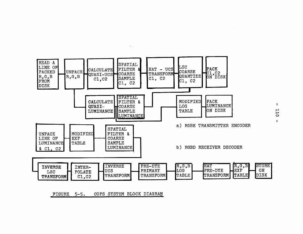
HH0

a) RGBE TRANSMITTER ENCODER

b) RGBD RECEIVER DECODER

FIGURE 5-5. COPS SYSTEM BLOCK DIAGRAY

- 111 -

blue separations with computer generated registration points

and a color scale.

The pictures are coded and decoded on a line-by-line

basis and a significant percentage of the processing time is

due to disk transfers. Several look-up tables are used to

trade off memory space for speed, thereby minimizing the time

required for long transforms performed at every pel, which

require transcendental functions and multiplications. Tables

of log and exponential conversion and red, green, and blue

luminances are included as well as chrominance conversion

tables.

The various programs in the COPS software package fall

into one of four categories:

1. Executive system software written in FORTRAN

2. Bit manipulation packing, unpacking, scaling, and

data transfer routines written in MACRO assembly

language

3. Transforms operating on each pel written in MACRO

4. Transforms operating on the coarsely sampled, filtered

pels (1/16 the total number of pels) written in FORTRAN

Practical implementation of real time stream processing

necessitates a judicious choice of algorithms which share

operations and combine several transformation steps into one.

The COPS system is much slower than an optimum fixed system

written entirely in MACRO, because there must be provisions

for trying different transforms and setting various parameters.

- 112 -

Also, many frequently modified arithmetic routines are written in

FORTRAN which compiles very inefficiently on the PDP-9. The

capabilities of the PDP-9 central processing unit are quite

primitive, compared to modern microprocessors fitted with a

high speed arithmetic processor. The absence of multiple

registers and of a stack memory results in very inefficient

transferring of data in multiple argument algorithms. However,

the optimum all-MACRO version of the encoder and decoder run

on the PDP-9 would operate in real time (i.e., pel processing

operations with filtering and packing overhead are under 500 sec.).

5.4 Reconstruction of Color Pictures

Red, green, and blue separations are reproduced on a

Laserphoto facsimile receiver. The receiver uses a scanning

laser beam to expose dry silver paper which is heat developed

in a matter of seconds to yield a fairly high resolution print

with a 0.2 to 1.8 density range. The receiver tone scale is

not very stable or linear in density or reflectance and so a

table of look-up values must be generated to linearize the

tone scale. A computer generated stepwedge is measured on a

digital reflectance densitometer. The density levels are fed

into a tone scale correction program which linearly interpolates

reflectances according to:

-D+D . -D +D .10 min - 10 max min (5.4-1)

-D +D .(41 - 10 max min

- 113 -

The computer translates the red, green, or blue six-bit

pel value into an eight-bit reflectance value which is sent

to the facsimile interface (figure 5-4).

Computer registered separations cannot be easily viewed

in an optical additive viewer because the intense light flux

necessary to overcome filter and lens losses would continue to

develop the unfixed dry silver paper. In other types of

additive viewers, the prints must be registered each time they

are viewed. The most important reason not to use an additive

viewer, however, is that facsimile separations are always

reproduced by a subtractive dye process. Part of the design

of the facsimile system requires a good understanding of the

dye reproduction system. Even if additively viewed, the pictures

must eventually be photographically reproduced.

Color photographic reproduction of the separations is

accomplished by multiply exposing the pin registered separations

through red (W29), green (W61), and blue (W47B) filters which

are chosen so that only one emulsion layer will be sensitized

at a time. The illumination is provided by two 3200*K bulbs

mounted in bowl reflectors, and the lamp voltage is regulated

by a variac. A Nikon camera back is used with a Schneider

leaf shutter copy lens to eliminate any movement of the 35mm

frame during multiple exposures. By both calculation (using

the illuminant spectra and the filters, and taking sensitivity

spectral curves) and experiment, the exposure ratios for the

three separations are calculated.

VI. Color

6.1:

6.2:

6.3:

- 114 -

Picture Evaluation and Conclusions

Subjective Analysis of Compressed Color Pictures

Topics for Further Research

Conclusion

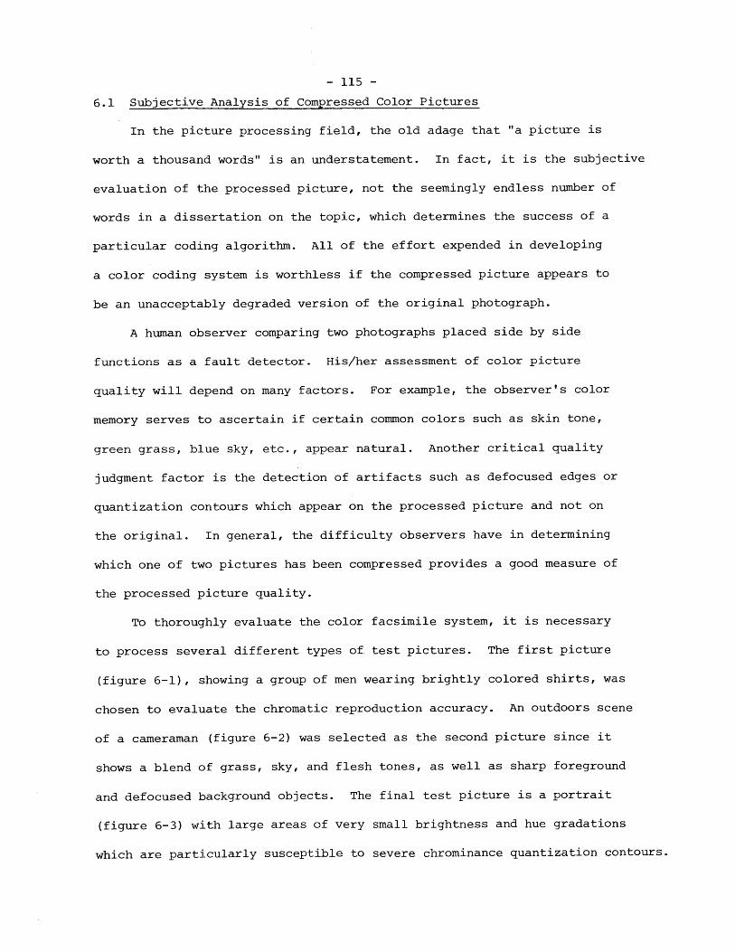
- 115 -

6.1 Subjective Analysis of Compressed Color Pictures

In the picture processing field, the old adage that "a picture is

worth a thousand words" is an understatement. In fact, it is the subjective

evaluation of the processed picture, not the seemingly endless number of

words in a dissertation on the topic, which determines the success of a

particular coding algorithm. All of the effort expended in developing

a color coding system is worthless if the compressed picture appears to

be an unacceptably degraded version of the original photograph.

A human observer comparing two photographs placed side by side

functions as a fault detector. His/her assessment of color picture

quality will depend on many factors. For example, the observer's color

memory serves to ascertain if certain common colors such as skin tone,

green grass, blue sky, etc., appear natural. Another critical quality

judgment factor is the detection of artifacts such as defocused edges or

quantization contours which appear on the processed picture and not on

the original. In general, the difficulty observers have in determining

which one of two pictures has been compressed provides a good measure of

the processed picture quality.

To thoroughly evaluate the color facsimile system, it is necessary

to process several different types of test pictures. The first picture

(figure 6-1), showing a group of men wearing brightly colored shirts, was

chosen to evaluate the chromatic reproduction accuracy. An outdoors scene

of a cameraman (figure 6-2) was selected as the second picture since it

shows a blend of grass, sky, and flesh tones, as well as sharp foreground

and defocused background objects. The final test picture is a portrait

(figure 6-3) with large areas of very small brightness and hue gradations

which are particularly susceptible to severe chrominance quantization contours.

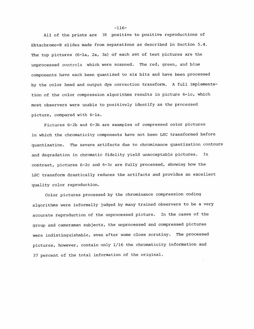
-116-

All of the prints are 3R positive to positive reproductions of

Ektachrome-B slides made from separations as described in Section 5.4.

The top pictures (6-la, 2a, 3a) of each set of test pictures are the

unprocessed controls which were scanned. The red, green, and blue

components have each been quantized to six bits and have been processed

by the color head and output dye correction transform. A full implementa-

tion of the color compression algorithms results in picture 6-lc, which

most observers were unable to positively identify as the processed

picture, compared with 6-la.

Pictures 6-2b and 6-3b are examples of compressed color pictures

in which the chromaticity components have not been LSC transformed before

quantization. The severe artifacts due to chrominance quantization contours

and degradation in chromatic fidelity yield unacceptable pictures. In

contrast, pictures 6-2c and 6-3c are fully processed, showing how the

LSC transform drastically reduces the artifacts and provides an excellent

quality color reproduction.

Color pictures processed by the chrominance compression coding

algorithms were informally judged by many trained observers to be a very

accurate reproduction of the unprocessed picture. In the cases of the

group and cameraman subjects, the unprocessed and compressed pictures

were indistinguishable, even after some close scrutiny. The processed

pictures, however, contain only 1/16 the chromaticity information and

37 percent of the total information of the original.

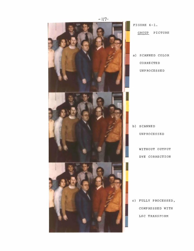
- 117-FIGURE 6-1.

GROUP PICTURE

a) SCANNED COLOR

CORRECTED

UNPROCESSED

b) SCANNED

UNPROCESSED

WITHOUT OUTPUT

DYE CORRECTION

c) FULLY PROCESSED,

COMPRESSED WITH

LSC TRANSFORM

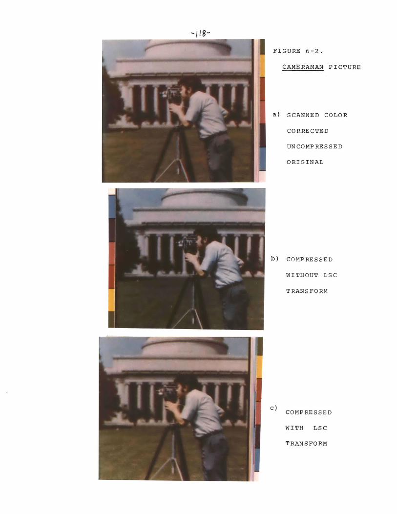
-l8-

FIGURE 6-2.

CAMERAMAN PICTURE

a) SCANNED COLOR

CORRECTED

UNCOMPRESSED

ORIGINAL

b) COMPRESSED

WITHOUT LSC

TRANSFORM

c) COMPRESSED

WITH LSC

TRANSFORM

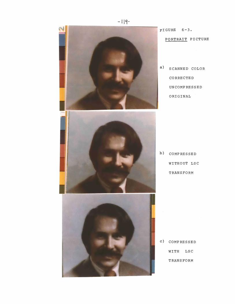
-119-

FIGURE 6-3.

PORTRAIT PICTURE

a) SCANNED COLOR

CORRECTED

UNCOMPRESSED

ORIGINAL

b) COMPRESSED

WITHOUT LSC

TRANSFORM

C) COMPRESSED

WITH LSC

TRANSFORM

-120-6.2 Topics For Further Research

-In any research project of the scope of this dissertation, many

interesting theoretical and design problems must be lightly treated or

not completely optimized in the interest of a reasonable time schedule.

Although the color facsimile system developed in this thesis is quite

complete, in that color pictures were scanned, compressed, and reproduced

with excellent quality, there are a number of areas for future work.

At the present time, the author, himself, is working on a number of

these problems:

1) The LSC transform provides excellent reduction of chrominance

quantization noise, but for certain critical test pictures, some

contour artifacts are noted. Techniques exist for reducing these

contours by adding pseudo-random noise with half of the least

significant bit amplitude before the coarse quantizer, and

subtracting out the noise at the output. These Robert's noise

techniques will no doubt remove whatever contour artifacts presently

exist in some pictures.

2) At the present time, if the color facsimile system were put into

operation, the receiver decoder electronics would have to be connected

to three monochrome facsimile receivers to produce the red, green, and

blue separations. It is feasible to construct a laser receiver, using

dry silver, heat developed paper, which uses a single laser and mirror

galvanometer deflection system to simultaneously scan three sections of

a piece of dry silver paper through a triple beam splitter. The beams

would be individually modulated by three electro-optical light

-121-modulators.

3) As was mentioned in chapter two, the chromaticity components cannot

be optimally encoded due to the nonrectangular region of reproducible

colors. If the components were quantized to five bits instead of four, then

the resulting ten bits of chrominance information might only represent

eight bits of valid codewords. The ten bits of data can be sent to an

8K bit read only memory, which would output a new set of single eight

bit code words which would all be valid.

4) The HAT transform techniques for correcting the color head sensor

response functions and most important, for correcting for the unwanted

absorptions of the subtractive dyes, can be further optimized. In the

caes of the dye correction, the trade-offs are between accurately

reproduced pale colors with large errors for the magenta dye at high

densities, or accurate reproduction of the darker, more saturated

colors. In addition to determining the quadrant and slope of the chrom-

aticity components, one might also determine the distance from the

white point. In this way, twelve transforms can be derived, six for

the pale colors and six for the darker colors.

5) In the facsimile receiver, the luminance must be again filtered to

determine the LSC transformed inverse values of the coded chromaticity

components. This filtering requires a twelve line luminance buffer

memory in the receiver. Techniques may exist for somehow encoding the

filtered luminance information in one of sixteen high resolution

luminance pels as a dithered position. In this way the receiver

luminance buffer memory could be reduced to four lines.

6.3 Conclusions

Starting with a few constraints based on psychophysical data, the

existing facsimile system specifications, a basic model of the photo-

graphic process, and data for a particular photographic material, this

dissertation has developed a practical facsimile system which produces

high quality compressed color pictures. The choice of the 16:1 com-

pression ratio was dictated by the requirement of encoding the color

information into the retrace blanking region of standard monochrome

facsimile signal. The possibility of such a compression was established

in earlier research. The major contributions of original work in this

dissertation result from examining in detail the four steps in the color

processing system which appeared to most severely limit the color

picture quality:

1) The efficiency of chrominance codeword utilization is greatly

improved by the LSC transform developed in Chapter Two.

2) The concept of overall filter function developed in Chapter

Three permits parameters to be chosen which minimize artifacts

resulting from chrominance spatial filtering, coarse sampling,

and interpolation.

3) The outputs of three colorimetrically inaccurate color head

functions are transformed to values which closely approximate the

tristimulus components. The transform is separately optimized by

both the luminance (by least mean square technique) and the

chrominance (by piecewise linear transformations).

4) Accurate photographic reproduction of colorimetric values is

accomplished by a color primary transform and a piecewise linear

density domain transform which together approximate the inverse

transform of the photographic process.

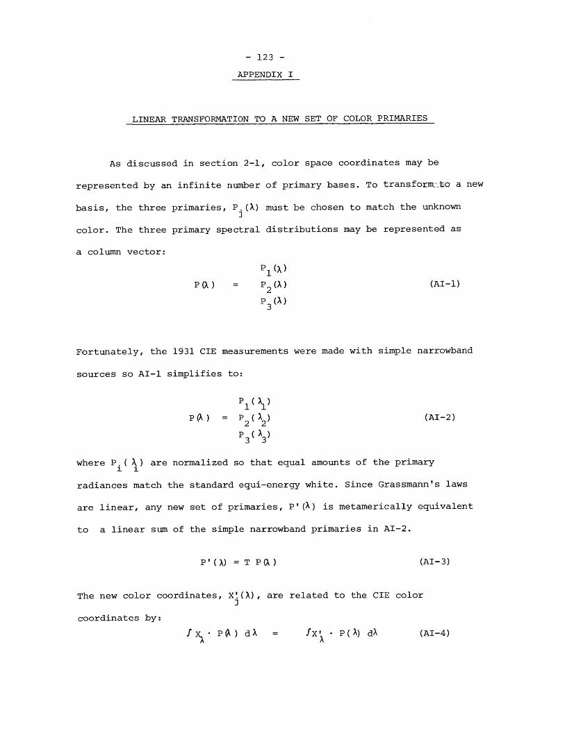
- 123 -

APPENDIX I

LINEAR TRANSFORMATION TO A NEW SET OF COLOR PRIMARIES

As discussed in section 2-1, color space coordinates may be

represented by an infinite number of primary bases. To transform:.to a new

basis, the three primaries, P.(X) must be chosen to match the unknownJ

color. The three primary spectral distributions may be represented as

a column vector:

P 1W

P(X) = 2 (A) (AI-l)

P (A)

Fortunately, the 1931 CIE measurements were made with simple narrowband

sources so AI-l simplifies to:

P ( j

P(A) = P (A) (AI-2)2 2

P (A )3 3

where P. ( A) are normalized so that equal amounts of the primary1 1

radiances match the standard equi-energy white. Since Grassmann's laws

are linear, any new set of primaries, P' (A) is metamerically equivalent

to a linear sum of the simple narrowband primaries in AI-2.

P'(A) = T P(X) (AI-3)

The new color coordinates, X'(A), are related to the CIE colorJ

coordinates by:

f X - P ) dA f X' - P(A) dA (AI-4)

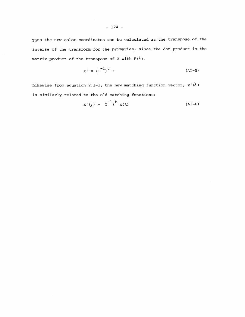
- 124 -

Thus the new color coordinates can be calculated as the transpose of the

inverse of the transform for the primaries, since the dot product is the

matrix product of the transpose of X with P(X).

X' = (T~1)t X (AI-5)

Likewise from equation 2.1-1, the new matching function vector, x' (A)

is similarly related to the old matching functions:

x' (X ) = (T 1) t x () (AI-6)

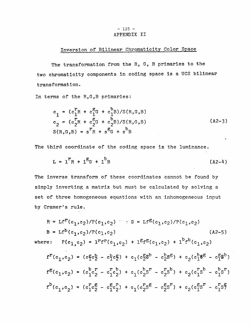
- 125 -

APPENDIX II

Inversion of Bilinear Chromaticity Color Space

The transformation from the R, G, B primaries to the

two chromaticity components in coding space is a UCS bilinear

transformation.

In terms of the RG,B primaries:

c1 = (cR + cgG + c B)/S(R,G,B)

c = (c R + c G + c bB)/S(RG,B) (A2-3)2 2 2 2

S(R,G,B) = srR + s G + s B

The third coordinate of the coding space is the luminance.

L = R + 1 G + lbB (A2-4)

The inverse transform of these coordinates cannot be found by

simply inverting a matrix but must be calculated by solving a

set of three homogeneous equations with an inhomogeneous input

by Cramer's rule.

R)= Lfr(c1,c2 )/P(c1,c) G = Lfg(cl,c2 )/P(cl,c2 )

B = Lfb(ci,c2 )/P(clc 2 ) (A2-5)

where: P(cic 2) = lrfr(cl,c 2 ) + lfg(cl,c2 ) + lbfb(clc 2 )

fr(c 1,c2 ) = (cc - c c ) + c(cb - S) + c2 (cb8 - cg b

f(cb,c 2 ) (c c - c c ) + c (cb S - c S ) + c2 (crS - c S r

f b (c,c 2 ) = (c(c - cgcrc c Sr) + c2 - cS5

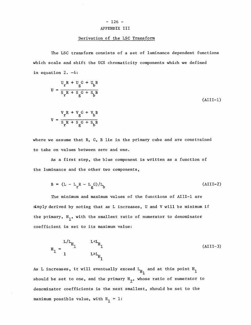
- 126 -

APPENDIX III

Derivation of the LSC Transform

The LSC transform consists of a set of luminance dependent functions

which scale and shift the UCS chromaticity components which we defined

in equation 2. -4:

U rR + U 9G + U bBr g bS R + S G + S Br g b

(AIII-1)

V R + V G + V Br g b

S R + S G + S Br g b

where we assume that R, G, B lie in the primary cube and are constrained

to take on values between zero and one.

As a first step, the blue component is written as a function of

the luminance and the other two components,

B = (L - L rR - L G) /Lb (AIII-2)

The minimum and maximum values of the functions of AIII-1 are

simply derived by noting that as L increases, U and V will be minimum if

the primary, H 1 , with the smallest ratio of numerator to denominator

coefficient is set to its maximum value:

L/L L<L1HHH1 1 (AIII-3)

1 L>LH

As L increases, it will eventually exceed and at this point Hl

should be set to one, and the primary H2, whose ratio of numerator to

denominator coefficients is the next smallest, should be set to the

maximum possible value, with H = 1:

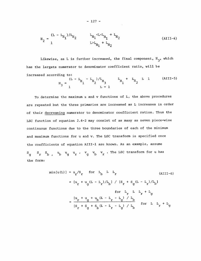
- 127 -

(L - LH )/LH21 2

LH <L<LH + LH

L + LH2

Likewise, as L is further increased, the final component, H 3, which

has the largets numerator to denominator coefficient ratio, will be

increased according to:

H =3

(L - L - L )/LHH H1 2 3

1 L=

L + LH L 1HH1 2

(AIII-5)

1

To determine the maximum u and v functions of L, the above procedures

are repeated but the three primaries are increased as L increases in order

of their decreasing numerator to denominator coefficient ratios. Thus the

LSC function of equation 2.4-2 may consist of as many as seven piece-wise

continuous functions due to the three boundaries of each of the minimum

and maximum functions for u and v. The LSC transform is specified once

the coefficients of equation AIII-l are known. As an example, assume

S S S b u u , v v v . The LSC transform for u hasg r b, b g r g b r

the form:

min[u(L)] = ur Sr for Lb L Lr

= [u + u (L - L )/L] / [S + S (L - L )/Lb]r g r b r g rfb

for L L L + Lr r g

[u + u + ub(L - L - L ) / Lr g L r g b

[S + S + S(L -L - L )/L for g b r g b

(AIII-6)

+ Lr g

H =2

(AIII-4)

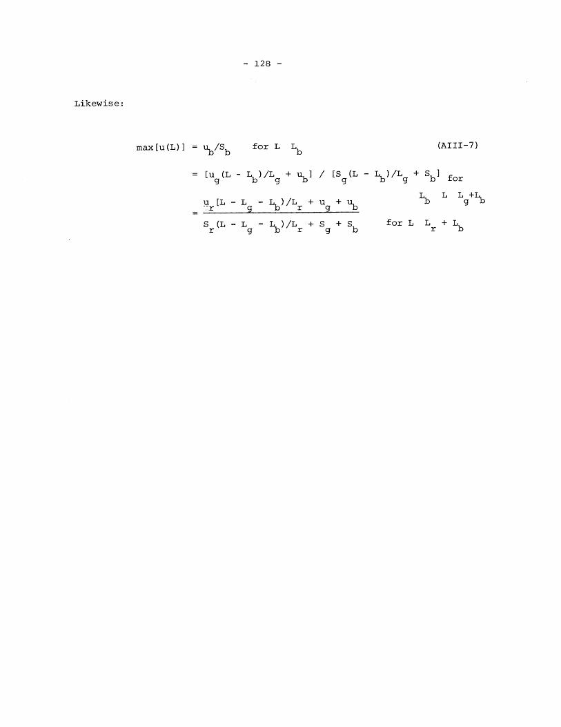
- 128 -

Likewise:

max [u (L)] = ub/Sb for L Lb (AIII-7)

[u g(L - Lb)/L + ub] / [S (L - Lb)/L + Sb for

u r [L - L - Lb)/Lr + u + L L L +Lb

S (L - L - Lb)/L + S + S for L L + Lr g b r g b r b

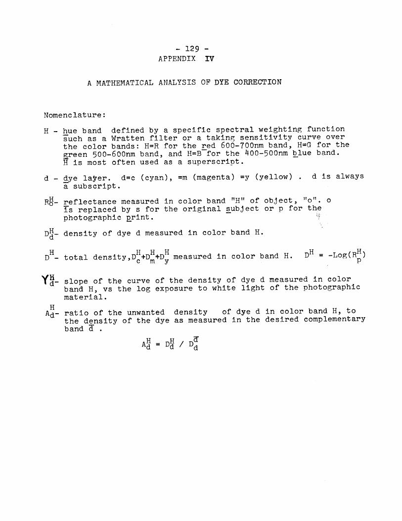
- 129 -APPENDIX IV

A MATHEMATICAL ANALYSIS OF DYE CORRECTION

Nomenclature:

H - hue band defined by a specific spectral weighting function

such as a Wratten filter or a taking sensitivity curve over

the color bands: H=R for the red 600-700nm band, H=G for the

green 500-600nm band, and H=B for the 400-500nm blue band.

H is most often used as a superscript.

d - dye layer. d=c (cyan), =m (magenta) =y (yellow) . d is always

a subscript.

Rd- reflectance measured in color band "H" of object., "O". 0is replaced by s for the original subject or p for thephotographic print.

DH- density of dye d measured in color band H.d

D H- total density,D +D +D measured in color band H. DH = -Log(RH)cm y p

- slope of the curve of the density of dye d measured in color

band H, vs the log exposure to white light of the photographicmaterial.

HAd- ratio of the unwanted density of dye d in color band H, to

the density of the dye as measured in the desired complementaryband d .

A = DH / D

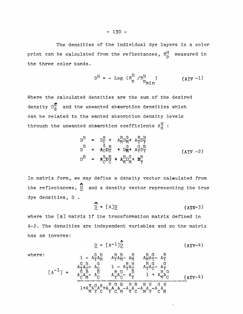
- 130 -

The densities of the individual dye layers in a color

print can be calculated from the reflectances, RH measured inp

the three color bands.

DH - Log (RH /RH ) (AIV -1)p Pmin

Where the calculated densities are the sum of the desired

density D and the unwanted absorption densities which

can be related to the wanted absorption density levels

through the unwanted absorption coefficients Ad

DR = D + ARD + A Dy

G G R G G BD = ACD0 + DM+ AyDy (AIV .-2)

DB = ADR + A BD+ D

In matrix form, we may define a density vector caleulated from

Athe reflectances, D and a density vector representing the true

dye densities, D .AD = [A]D (AIV-3)

where the [A] matrix if the transformation matrix defined in

A-2. The densities are independent variables and so the matrix

has an inverse:

D = [A- 1]D (AIV-4)

where: 1 AG AB AR AB_ R AR AG_ Rhe:1 - AyA AyA- AM AAY- Ay

1 A AB A 1 - AR A AR A Ay[A~- = A A-A A A - A B 1 + A A AC M C Y C Y M C (Aiv-4)

BRGB R GB R B B G G R1+AA A +A A A -A A -A A -A A

M Y C Y C M Y C M Y C M

- 131 -

Thus the density of each dye layer may be determined from the

negative logarithm of the color head reflectance measurements.

The AH are determined from the spectral responses of thed

filters, photodetectors, etc., and the dye reflectance functions

for a specific illumination. The A will therefore vary with

photographic material.

The filters should be chosen to be as narrow as

possible since the dye density functions are not block

functions and thus the shape of the reflectance spectral

characteristics changes with density level. The filters

must be wide enough so that electronic signal to noise

ratio does not limit the dynamic range of measurement.

The measurements of each dye density in the

three color bands results in nine contrast coefficients YdH

which relate the D densities to the log of the exposured H

E, of that particular emulsion layer. As with the Ad, a

matrix may be formed [y] = (yd

H H H H kHDd = Dd + yd Log eHE y d Log kd Ed dmin d

(AIV-5)

The total reflectance from the color print in color band

H may be calculated from the density in that color band:

H H [D - DH (AIV-6)R = a [10 min

-132-The primary requirement of any color process is that

neutral tones (greys) must reproduce as neutrals. The most

subjectively noticeable chromatic degradation results from not

preserving neutral balance. If the original subject reflectances

are normalized so that they are equal for achromatic points

(R = RG = RB), then neutral balance requires that the total

dye density measured in each color band is equal over the grey

scale. This can only be achieved if the total gamma coefficient

for each color band are equal.

R G BY =Y =( -7)

where:H

y - 2y( -8)d Id

The ratio of oney value to another is proportional to the

ratio of the dye densities for white light exposure in the

particular color bands for the particular dye layers.

1Y = DH, D H2Ydi d 2 dl d2

The neutrality condition forces the dye density gamma values

in the band of desired absorption to be unequal. This results

in the color of a particular dye varying with density. Thus the

reproduced hue and saturation level of a reproduced color will

vary with the luminance. This arises because the color is

determined by a ratio of reflectances, whereas the dye densities

are the negative logarthm of reflectance and the photograph

reflectances are exponential functions of the densities. As an

example oftthis non-linear effect, the purity of a blue object

can be formulated as a function of its luminance. One possible

- 133 -

measure of blue fidelity F(B) is the ratio of the blue to

yellow light reflected by a print reproduction of a

spectrally pure blue object.

B B kB DG = G kB~(I-0D = Log k L D Log k2L (AIV-10)

then: F(B) = R / R G = 10[-D - Dx] (AIV-ll)

or: F(B) = (L ) Y Y (AIV-12)

Since the H are non-negative, and B G the fidelitySnete d Y y tefdlt

decreases as the original luminance decreases. Thus a light

blue will reporduce more inaccurately, colorimetrically

speaking, then a dark blue. The light blue will be darker

and shifted toward the green. Thus to maximize the exponent

of AIV-12 the overall of the system must be increased.

The effective ratio of wanted to unwanted absorptions will

therefore be increased. The overall gamma cannot be increased

too much before the dynamic range of the reproduction material

is exceeded for a given input range of grey levels. Also

the achromatic colors are best reproduced with a gamma of

unity. The commonly chosen value is about 1.2 for reflectance

prints, and 1.8 for the much larger dynamic range of

transparencies.

The larger gamma in transparencies necessitates

a pre-dye correction transform (Chapter four) since when

a slide is again reproduced, the resulting gamma of 3.24

is unacceptably high.

- 134 -

APPENDIX V

COLOR TRANSFORM FOR NEW PRIMARIES WITH SPECIFIED CHROMATICITIES

In appendix I, the transform of the color coordinates for a new set

of primaries is derived. This appendix examines this transformation when

the new primaries are specified in the chromaticity plane. Knowing the

u and v coordinates for each of the three new primaries specifies six of

the nine coefficients of the transform of equation AI-3. The other

three coefficients are determined from the constraint of the luminosity

coefficients which requires the new color coordinates R', G', B' to each

equal one, when the CIE R, G, B coordinates each equal one.

From AIII-l, specifying u. and v. at each "i" new primary pointi 1

determines the values of the G' and B' coordinates in terms of the

red coordinate. By solving the two equations in two unknowns, G. and B.1 1

for each of the three new primaries can be expressed in terms of R..

R. (u.S - D ) = G. (u - u.S ) + B. (u - u.Sbi i r r i g ig iUb ib

(AV-l)

R. (v.s - v ) = G. (v - v.S ) + B. (v - v.S)i i r r i g i g i b i b

Thus the transform to the new primaries is of the form:

-1 T T21S11

T = 1 T 12T 22 K (AV-2)

ja1 13 T231

where the matrix is known up to a constant multiplier.

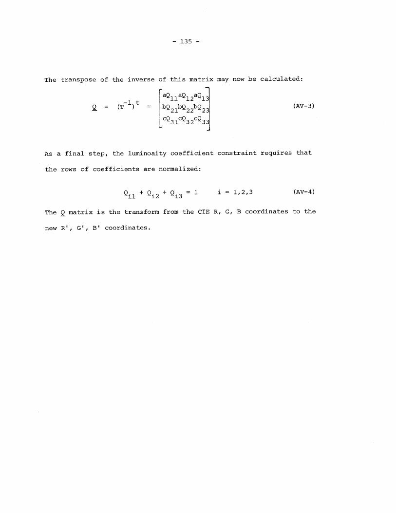
- 135 -

The transpose of the inverse of this matrix may now be calculated:

aQ 1 aQ1 2aQ

Q = (T) = bQ 2 1bQ 2 2bQ23 (AV-3)

cQ 3 1cQ 3 2 cQ3 3j

As a final step, the luminoaity coefficient constraint requires that

the rows of coefficients are normalized:

Q 1 + Qi2 +i = 1 i = 1,2,3 (AV-4)

The Q matrix is the transform from the CIE R, G, B coordinates to the

new R', G', B' coordinates.

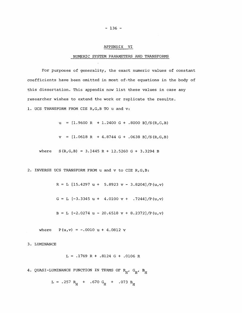
- 136 -

APPENDIX VI

NUMERIC SYSTEM PARAMETERS AND TRANSFORMS

For purposes of generality, the exact numeric values of constant

coefficients have been omitted in most of'the equations in the body of

this dissertation. This appendix now list these values in case any

researcher wishes to extend the work or replicate the results.

1. UCS TRANSFORM FROM CIE R,G,B TO u and v:

u = [1.9600 R + 1.2400 G + .8000 B]/S(R,G,B)

v = [1.0618 R + 4.8744 G + .0638 B]/S(R,G,B)

where S(R,G,B) = 3.1445 R + 12.5260 G + 3.3294 B

2. INVERSE UCS TRANSFORM FROM u and v to CIE R,G,B:

R = L [15.4297 u + 5.8923 v - 3.8204]/P(u,v)

G = L [-3.3345 u + 4.0100 v + .7244]/P(u,v)

B = L [-2.0274 u - 20.6518 v + 8.2372]/P(u,v)

where P(u,v) = -.0010 u + 4.0812 v

3. LUMINANCE

L = .1769 R + .8124 G + .0106 R

4. QUASI-LUMINANCE FUNCTION IN TERMS OF RH, GH, BH

L = .257 RH + .670 GH + .073 BH

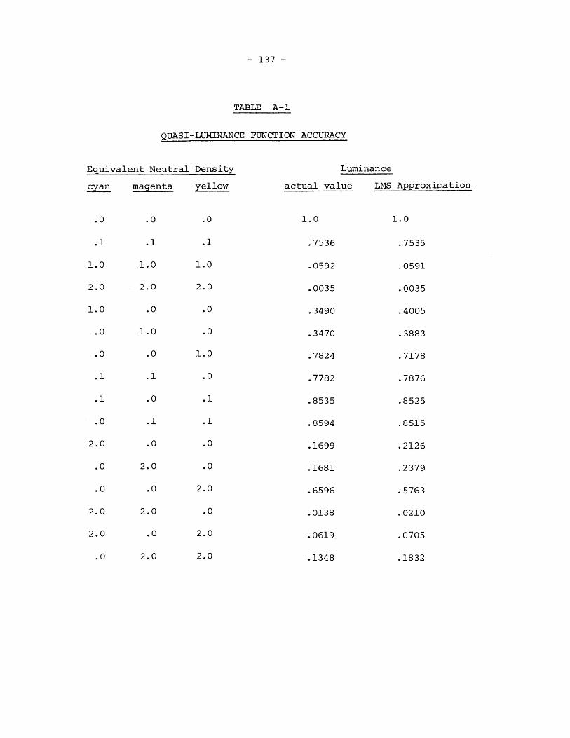
- 137 -

TABLE A-1

QUASI-LUMINANCE FUNCTION ACCURACY

Equivalent Neutral Density

cyan magenta yellow

.0

.1

.0

.1

1.0

2.0

1.0

2.0

1.0 .0

.0 1.0

.0

.1

.1

.0

.0

.1

.0

.1

.02.0

.0 2.0

.0 .0

2.02.0

2.0 .0

.0

.1

1.0

2.0

.0

.0

1.0

.0

.1

.1

.0

.0

2.0

.0

2.0

Luminance

actual value

1.0

.7536

.0592

.0035

.3490

.3470

.7824

.7782

.8535

.8594

.1699

.1681

.6596

.0138

.0619

2.0 .1348

LMS Approximation

1.0

.7535

.0591

.0035

.4005

.3883

.7178

.7876

.8525

.8515

.2126

.2379

.5763

.0210

.0705

.1832.0 2.0

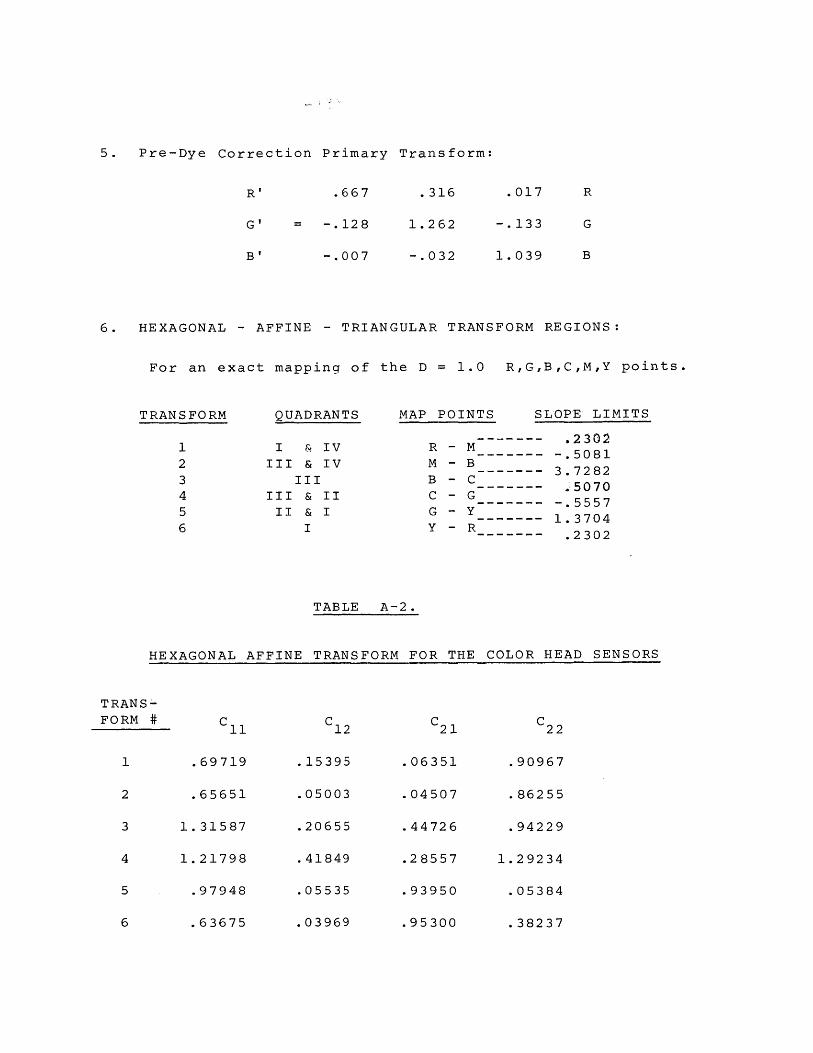
5. Pre-Dye Correction

B'

= -. 128

-. 007

6. HEXAGONAL - AFFINE - TRIANGULAR TRANSFORM REGIONS:

For an exact mapping of the D = 1.0 R,G,B,C,M,Y points.

TRANSFORM

1234

5

6

QUADRANTS

I & IV

III & IV

III

III & II

II & I

I

MAP POINTS SLOPE LIMITS

R -- .2302-.5081

M B B-------- 3.7282B-CC - ------- 5070

------- -. 5557G ------- 1.3704Y -R--------- .2302

TABLE A-2.

HEXAGONAL AFFINE TRANSFORM FOR THE COLOR HEAD SENSORS

TRANS-

FORM # C1 1

.69719

.65651

1.31587

1.21798

.97948

C1 2

.15395

.05003

.20655

.41849

.05535

C2 1

.06351

.04507

.44726

.28557

.93950

.03969 .95300

C2 2

.90967

.86255

.94229

1.29234

.05384

.38237

.667 .316

1.262

-. 032

.017

-. 133

1.039

R

G

B

1

2

3

4

5

Primary Transform:

6 .63675

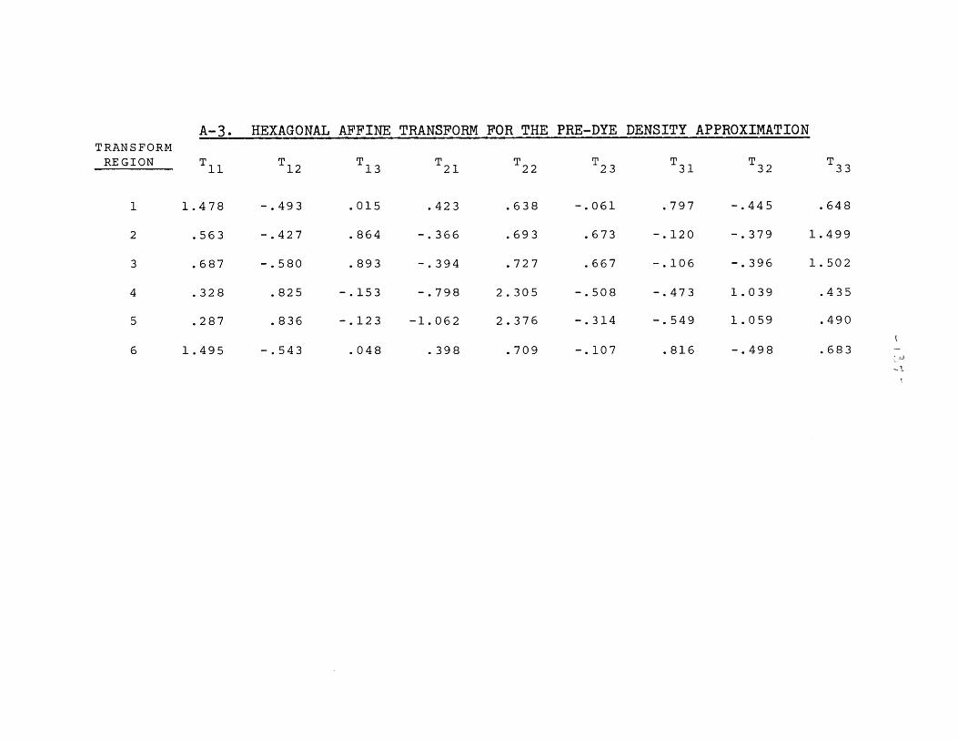
TRANSFORMREGION

1

2

3

4

5

6

A-3.

T 11

1.478

.563

.687

.328

.287

1.495

HEXAGONAL

T 12

-. 493

-. 427

-. 580

.825

.836

-. 543

AFFINE

T13

.015

.864

.893

-. 153

-. 123

.048

TRANSFORM

T21

.423

-. 366

-. 394

-. 798

-1.062

.398

FOR THE

T22

2

2

.638

.693

.727

.305

.376

.709

PRE-DYE

23

-. 061

.673

.667

-. 508

-. 314

-. 107

DENSITY APPROXIMATION

31 T32

797

120

106

473

549

816

-. 445

-. 379

-. 396

1.039

1.059

-. 498

1

1

T33

.648

.499

.502

.435

.490

.683

- 140 -

REFERENCES

1. Yule, J.A.C., Principles of Color Reproduction, John Wiley &

Sons, Inc., New York, 1967.

2. Pugsley, P.C., Electronic Scanners in Colour Printing,

Electronics & Power, January 10, 1974.

3. Pratt, W.K., Spatial Transform Coding of Color Images, IEEE

Trans. on Communication Technology, December 1971, Vol. COM-

19, No. 6, pp. 980-992.

4. Fink, D.G., Television Engineering, 2nd ed., McGraw-Hill,

New York, 1952.

5. Wentworth, J.W., Color Television Engineering, McGraw-Hill,

New York, 1955.

6. McIlwain, K., Requisite Color Bandwidth for Simultaneous Color-

Television Systems, Proc. IRE, Vol. 40, No. 8, August 1952,

pp. 909-912.

7. Loughren, A.V., Psychophysical and Electrical Foundations of

Color Television, Proc. IRE, January 1954, pp. 9-11.

8. Schade, O.H., On the Quality of Color Television Images and

the Perception of Color Detail," J. SMPTE, Vol. 67, 1958,

p. 801.

9. Brown, G.H., The Choice of Axes and Bandwidths for the

Chrominance Signals in NTSC Color Television, Proc. IRE,

January 1954, pp. 58-59.

10. Gronemann, U.F., Coding Color Pictures, MIT RLE report 422,

June 1964.

11. Wacks, K.P., Design of a Real Time Facsimile Transmission

System, MIT Ph.D. Thesis, 1973.

12. Legrand, Y., Light, Colour and Vision, Chapman and Hall Ltd.,

London, Copy 1957.

13. Bouma, P.J., Physical Aspects of Colour, N. V. Philips

Gloeilampenfabrieken, Eindhonen (Netherlands), 1947.

14. Kelly, D.H., Spatio-temporal Frequency Characteristics of

Color-Vision Mechanisms, J. Opt. Soc. Am., Vol. 64, July

1974, pp. 983-990.

- 141 -

15. Wintringham, W.T., Color Television and Colorimetry, Proc. IRE,October 1951, pp. 1135-1172.

16. Stockham, T.G., Jr., The Importance of Nonlinear Image Enhance-

ment in Visual Prosthesis Design, Visual Prosthesis, AcademicPress, 1971, pp. 173-192.

17. Tretiak, O.J., The Picture Sampling Process, MIT ScD. ThesisElec. Eng., September 1963.

18. Judd, D.B., Estimation of Chromaticity Differences and Nearest

Color Temperature on the Standard 1931 ICI Colorimetric

Coordinate System, J. Res. Nat. Bur. Stds., Vol. 17, 1936,pp. 771-779.

19. Rubinstein, C.B. and Limb, J.O., Statistical Dependence Between

Components of a Differentially Quantized Color Signal, IEEE

Transactions on Communications, Vol. COM-20, No. 5, October

1972, pp. 890-899.

20. Committee on Colorimetry Optical Society of America, The Science

of Color, Thomas Y. Crowell Company, New York, 1953.

21. Willmer, E.N., Color of Small Objects, Nature, Vol. 153, June 24,

1944, pp. 774-775.

22. Middleton, W.E. and Holmes, M.C., The Apparent Colors of Surfaces

of Small Substance - A Preliminary Report," J. Opt. Soc. Am.,Vol. 39, July 1949, pp. 582-592.

23. Luckiesh, M., The Dependence of Visual Acuity on the Wavelength

of Light, Electronics World, Vol. 58, November 18, 1911, p. 1252.

24. Hartridge, H., The Change from Trichromatic to Dichromatic Vision

in the Human Retina, Nature, Vol. 155, June 2, 1945, pp. 657-662.

25. McIlwain, K. and Dean, C.E. (eds.), Principles of Color Television,

John Wiley & Sons, Inc., New York, 1956.

26. Hacking, K., The Relative Visibilities of Spatial Variations inLuminance and Chromaticity, BBC Research Report No. T-146,August 1965.

27. Ratcliff, F., Mach Bands: Quantitative Studies on Neural Networks

in the Retina, Holden Day, Inc., Copy 1965.

28. Green, D.G., The Contrast Sensitivity of the Colour Mechanisms ofthe Human Eye, J. Physiology (Great Britain), Vol. 196, 1967,pp. 415-429.

- 142 -

29. Fink, D.G. (ed.), Color Television Standards: Selected Papers and

Records, McGraw-Hill, New York, 1955.

30. Baldwin, M.W., Jr., Subjective Sharpness of Additive Color Pictures,

Proc. IRE, October 1951, pp. 1173-1176.

31. Petersen, D.P. and Middleton, D., Sampling and Reconstruction of

Wave-Number Limited Functions in N-Dimensional Euclidean Spaces,

Information and Control, Vol. 5, 1962, pp. 279-323.

32. Brown, W.M., Optimum Filtering of Sampled Data, IRE Trans. Info.

Theory, Vol. IT-7, October 1961, pp. 269-270.

33. Hardy, A.C. and Wurzburg, F.L., Jr., Color Correction in Color

Printing, J. Opt. Soc. Am., Vol. 38, No. 4, April 1948.

34. Hardy, A.C. and Wurzburg, F.L., Jr., The Theory of Three-Color

Reproduction, J. Opt. Soc. Am., Vol. 27, No. 7, July 1937,

pp. 227-240.

35. Friedman, J.S., History of Color Photography, The American Photo-

graphic Publishing Co., Boston, 1944.

36. Kodak Publication E-78, Sensitometric and Image Structure Data

for Kodak Color Films, CAT 178-6680.

37. Yule, J.A.C., Principles of Color Reproduction, John Wiley &

Sons, Inc., New York, 1967.

38. Miller, T.H., Masking: A Technique for Improving the Quality of

Color Reproductions, J. Soc. of Motion Picture & TV Engs.,

Vol. 52, February 1949, pp. 133-155.

39. Hanson, W.T., Jr., and Brewer, W.L., Subtractive Color Photography:

The Role of Masks, J. Opt. Soc. Am., Vol. 44, February 1954,

pp. 129-134.

40. MacAdam, D.L., Subtractive Color Mixture and Color Reproduction,

J. Opt. Soc. Am., Vol. 28, December 1938, p. 466.

- 143 -

BIOGRAPHICAL NOTE

Born in Brooklyn, New York on August 9, 1945, Robert Solomon

attended Brooklyn Technical High School and then Polytechnic Institute of

Brooklyn where he received the B.E.E. summa cum laude. While he was an

NSF fellow he received the S.M. and Engineer degrees in electrical

engineering at M.I.T. in 1968 and 1970. From 1970 until 1974 he worked on

a laser facsimile transmitter and receiver and various color facsimile

hardware and theoretical projects. For the past seven years, he has been

a senior development engineer and project leader at General Radio Company,

where he developed various audio spectrum analyzer instruments and systems

using analog and FFT digital processing techniques and also conducted

research on interactive color display systems. In addition, he has

conducted much private research in his consultant practice in the areas

of video instrumentation and special effects, color reproduction, biomedical

instrumentation, and microprocessor systems.

Robert Solomon is a member and past chapter president of both

Tau Beta Pi and Eta Cappa Nu, and a member of Sigma Xi, the IEEE, and the

Optical Society of America. He has had accepted for publication and

presentation several papers in his areas of expertise.