COLLOIDAL CDSE/ZNS, PBSE AND PBS QUANTUM

DOTS FOR USE IN APPLICATIONS

A Dissertation

Presented to the Faculty of the Graduate School

of Cornell University

in Partial Fulfillment of the Requirements for the Degree of

Doctor of Philosophy

by

Stephen William Clark

January 2006

c© 2006 Stephen William Clark

ALL RIGHTS RESERVED

COLLOIDAL CDSE/ZNS, PBSE AND PBS QUANTUM DOTS FOR USE IN

APPLICATIONS

Stephen William Clark, Ph.D.

Cornell University 2006

Colloidal semiconductor quantum dots are novel materials whose electronic and

optical properties can be greatly enhanced from the bulk semiconductor proper-

ties by quantum confinement. A brief introduction to colloidal quantum dots and

the effect of size on its electronic and optical properties will be given. CdSe/ZnS,

PbS, and PbSe quantum dots will be described in more detail with regards to the

research done in this dissertation. CdSe/ZnS quantum dots have luminescence

that can be tuned in the visible, making them particularly suited for fluorescent

labels in biological applications. In particular, their potential use as voltage sen-

sors to detect cell membrane potentials and sphingosine phosphorylation will be

discussed. PbS and PbSe quantum dots emit in the near infrared, wavelengths

that are important to telecommunications. Their small third-order nonlinearity

and relatively long (microsecond) lifetimes will be discussed in terms of dielectric

screening. Fluoresence resonant energy transfer between PbS quantum dots will

also be discussed.

BIOGRAPHICAL SKETCH

Stephen Clark was born in Illinois in 1976. After high school he attended the

University of Illinois at Urbana-Champaign. In 1998, he graduated with a B.S.

in Physics. Soon after, he left to attend graduate school at Cornell University in

Ithaca, New York.

iii

ACKNOWLEDGEMENTS

I would like to acknowledge my advisor Frank Wise, my committee members Watt

Webb and Piet Brouwer, my previous advisors/employers Wilson Ho, John Sulli-

van, and Thomas Friedmann, my colleagues Andrew Perrella, Jason Petta, Kale

Beckwitt, Jeff Harbold, Omer Ilday, Hyungsik Lim, Byun-Ryool Hyun, Yi-Fan

Chen, Peer Fisher, Dan Larson, Warren Zipfel and the rest of Webb group, and

the rest of the people I worked with, my brother Andrew, my grandparents, and

anyone else who would like to be acknowledged.

I would also like to acknowledge the funding support. Most of the CdSe

work was sponsored by the Defense Advanced Research Projects Agency under

grant MDA972-00-1-0021. The lead salt work was sponsored by Nanoscale Sci-

ence and Engineering Initiative of the National Science Foundation under NSF

Award # EEC-0117770 and the New York State Office of Science, Technology and

Academic Research under NYSTAR Contract # C020071. The content of this

dissertation does not necessarily reflect the position of the U.S. government, and

no official endorsement should be inferred.

iv

TABLE OF CONTENTS

1 Introduction 11.1 Colloidal Semiconductor Nanocrystals . . . . . . . . . . . . . . . . . 11.2 Organization of the Dissertation . . . . . . . . . . . . . . . . . . . . 7

2 CdSe/ZnS Quantum Dots in Biology 82.1 Introduction . . . . . . . . . . . . . . . . . . . . . . . . . . . . . . . 82.2 Initial Characterization . . . . . . . . . . . . . . . . . . . . . . . . . 92.3 Membrane Potential Measurements . . . . . . . . . . . . . . . . . . 142.4 Stark Effect Measurements . . . . . . . . . . . . . . . . . . . . . . . 152.5 Black Lipid Membranes . . . . . . . . . . . . . . . . . . . . . . . . 162.6 Giant Unilamellar Vesicles . . . . . . . . . . . . . . . . . . . . . . . 172.7 Rat Basophilic Leukemia Cells and Gramicidin . . . . . . . . . . . . 182.8 Conclusion . . . . . . . . . . . . . . . . . . . . . . . . . . . . . . . . 19

3 CdSe/ZnS Quantum Dots for Studies of Sphingolipid Metabolism 203.1 Sphingolipid Metabolism . . . . . . . . . . . . . . . . . . . . . . . . 203.2 Encapsulating Quantum Dots with Sphingosine . . . . . . . . . . . 233.3 Sphingosine Phosphorylation Experiments . . . . . . . . . . . . . . 293.4 Conclusion . . . . . . . . . . . . . . . . . . . . . . . . . . . . . . . . 29

4 CdSe/ZnS Quantum Dots in Biology, Conclusion 324.1 Revisiting the Membrane Potential Experiments . . . . . . . . . . . 324.2 The Aplysia experiment . . . . . . . . . . . . . . . . . . . . . . . . 334.3 Conclusion . . . . . . . . . . . . . . . . . . . . . . . . . . . . . . . . 35

5 Nonlinear Measurements of PbSe Quantum Dots 375.1 Introduction . . . . . . . . . . . . . . . . . . . . . . . . . . . . . . . 375.2 The Z-scan . . . . . . . . . . . . . . . . . . . . . . . . . . . . . . . 385.3 The Samples . . . . . . . . . . . . . . . . . . . . . . . . . . . . . . . 405.4 Experimental Results . . . . . . . . . . . . . . . . . . . . . . . . . . 425.5 Conclusion . . . . . . . . . . . . . . . . . . . . . . . . . . . . . . . . 46

6 The Photoluminscence Lifetime and Dielectric Screening of PbSQuantum Dots 476.1 Introduction . . . . . . . . . . . . . . . . . . . . . . . . . . . . . . . 476.2 Lifetime Experiments . . . . . . . . . . . . . . . . . . . . . . . . . . 476.3 Fluorescence Resonant Energy Transfer . . . . . . . . . . . . . . . . 516.4 Conclusion . . . . . . . . . . . . . . . . . . . . . . . . . . . . . . . . 57

v

A Methods for Encapsulating Quantum Dots in lipids 60A.1 Introduction . . . . . . . . . . . . . . . . . . . . . . . . . . . . . . . 60A.2 Washing the Dots . . . . . . . . . . . . . . . . . . . . . . . . . . . . 60A.3 Encapsulating the Dots . . . . . . . . . . . . . . . . . . . . . . . . . 62A.4 Filtering the Dots . . . . . . . . . . . . . . . . . . . . . . . . . . . . 63

Bibliography 65

vi

LIST OF TABLES

A.1 Table of the different combinations of lipids that produced singlequantum dot micelles. . . . . . . . . . . . . . . . . . . . . . . . . . 63

vii

LIST OF FIGURES

1.1 Diagram of a general colloidal semiconductor quantum dot . . . . . 21.2 Density of states for an electron in an ideal bulk semiconductor

(top) and an ideal quantum dot (bottom) . . . . . . . . . . . . . . 31.3 Absorbance of a typical sample of PbSe quantum dots. The first

exciton peak is clearly visible at 990 nm. . . . . . . . . . . . . . . . 4

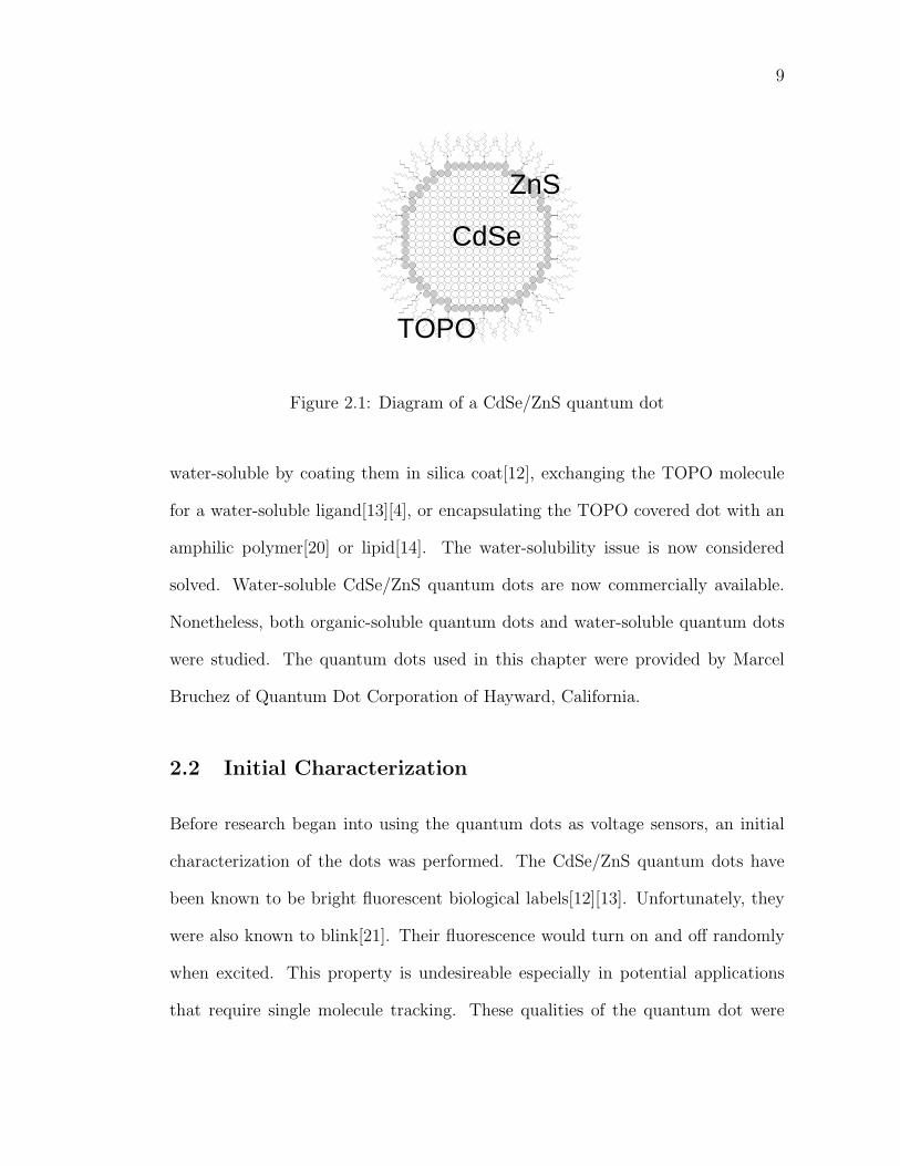
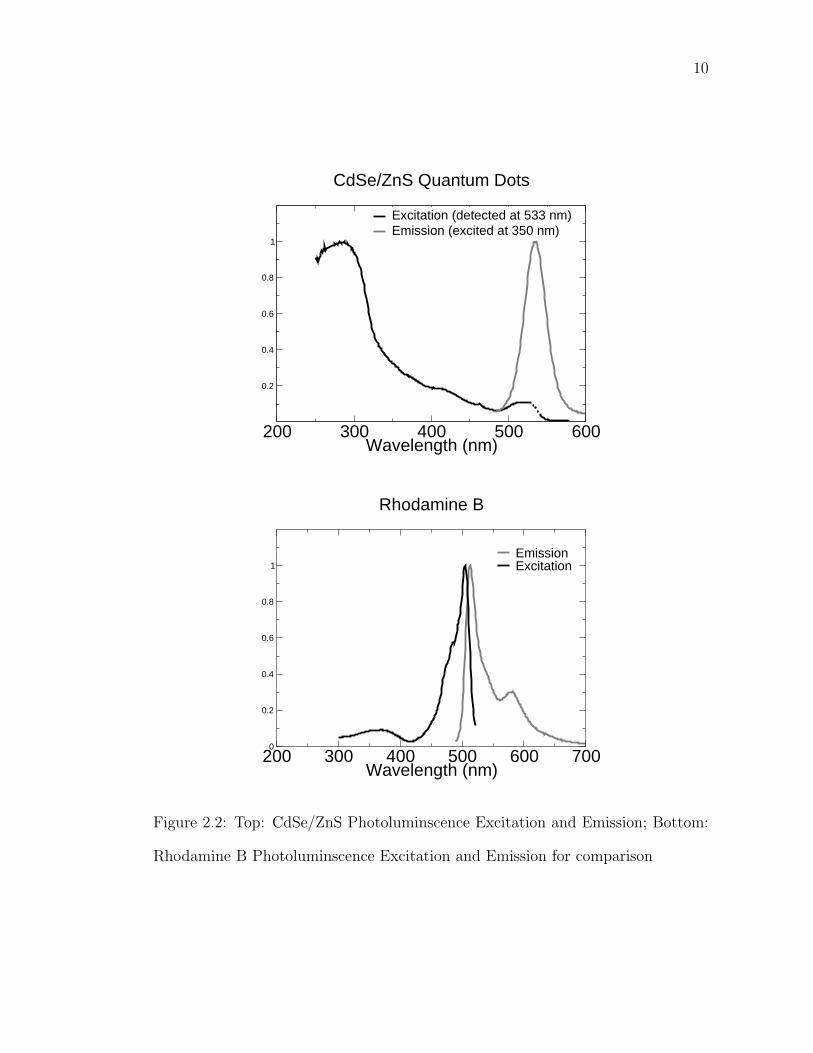
2.1 Diagram of a CdSe/ZnS quantum dot . . . . . . . . . . . . . . . . 92.2 Top: CdSe/ZnS Photoluminscence Excitation and Emission; Bot-

tom: Rhodamine B Photoluminscence Excitation and Emission forcomparison . . . . . . . . . . . . . . . . . . . . . . . . . . . . . . . 10

2.3 Top: Sample trace of photons counted versus time for a typicalFCS experiment. Bottom: Theoretical FCS curve for simple diffusion 12

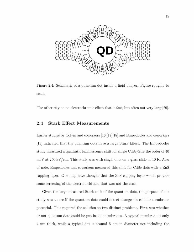
2.4 Schematic of a quantum dot inside a lipid bilayer. Figure roughlyto scale. . . . . . . . . . . . . . . . . . . . . . . . . . . . . . . . . . 15

3.1 Diagram of Sphingosine Phosphorylation . . . . . . . . . . . . . . . 213.2 Diagram of quantum dot with one sphingosine phosphorylated to

sphingosine-1-phosphate. Figure roughly to scale. . . . . . . . . . . 223.3 Chemical structure of the lipids used to encapsulate the quantum

dots. . . . . . . . . . . . . . . . . . . . . . . . . . . . . . . . . . . . 273.4 FCS curves of encapsulated dots. The fit to a single diffusion curve

and the hydrodynamic radius imply that the dots are in single dotmicelles, and are not aggregated. . . . . . . . . . . . . . . . . . . . 28

3.5 Data from the phosphorylation experiment. Top is data from dotswith 90% sphingosine. Middle is data from dots with 50% sphin-gosine. Bottom is data from dots with 5% sphingosine. . . . . . . . 30

4.1 Picture of Aplysia labeled with quantum dots encapsulated withlipids. . . . . . . . . . . . . . . . . . . . . . . . . . . . . . . . . . . 34

5.1 Diagram of the z-scan experiment. . . . . . . . . . . . . . . . . . . 385.2 Theoretical z-scan curves for both a positive and negative n2. . . . 395.3 Absorption of 1550 nm sample and spectra of the laser used for the

measurement. . . . . . . . . . . . . . . . . . . . . . . . . . . . . . . 415.4 Sample z-scan data. . . . . . . . . . . . . . . . . . . . . . . . . . . 425.5 Data of the peak change of transmittance of the z-scan versus time

from when the chopper opens and laser light is incident on the sample. 445.6 Diagram of the time resolved z-scan. . . . . . . . . . . . . . . . . . 45

6.1 Diagram of the experimental setup used to measure fluorescent life-times. . . . . . . . . . . . . . . . . . . . . . . . . . . . . . . . . . . 48

6.2 Data showing the variation of lifetime versus solvent. . . . . . . . . 506.3 Fluoresence shift in a film of quantum dots. . . . . . . . . . . . . . 52

viii

6.4 Spectrally and time resolved fluorescence of the quantum dot film. 546.5 Overlap of the emission from the 770 nm qauntum dots with the

absorbance of the 880 nm quantum dots. . . . . . . . . . . . . . . . 556.6 Fluorescence of the combination of dots in solvent (top) and in a

film (bottom). . . . . . . . . . . . . . . . . . . . . . . . . . . . . . 566.7 Spectrally and time resolved fluorescence of the quantum dot film. 58

ix

CHAPTER 1

INTRODUCTION

1.1 Colloidal Semiconductor Nanocrystals

Colloidal semiconductor nanocrystals or quantum dots are small pieces of semi-

conductor that are large enough to still have a crystal lattice but small enough

to exhibit quantum confinement effects. Small enough is determined by the Bohr

radius of the electron and hole of the bulk semiconductor. The electronic and

optical properties begin to change once the size of the nanocrystal becomes small

enough to confine the electron or hole.

Semiconductor quantum dots are usually one of two types. Epitaxial quantum

dots are grown or patterned on a surface. Colloidal quantum dots are grown in

solution from precusors. This thesis will only deal with colloidal quantum dots.

There are numerous ways to grow quantum dots in solution. The dots used in this

thesis are grown by the injection of organometallic reagents into a hot coordinating

solvent. This causes immediate nucleation. The quantum dots continue to increase

in size due to the process of Ostwald ripening (smaller nanocrystals are more

likely to disolve than the larger ones due to higher surface free energy). The size

is determined by when the growth is stopped. This process however does not

produce quantum dots of just one size. There is always a distribution of sizes. A

common distribution is 5%[1][2]. This distribution will cause the ensemble optical

properties to be inhomogenously broadened. Unfortunately, this inhomogenous

broadening greatly complicates extracting information on the quantum dots.

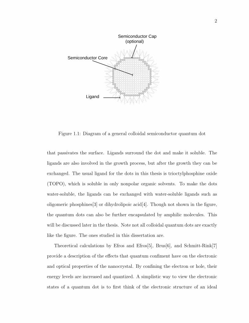
Figure 1.1 is a diagram of a general colloidal semiconductor quantum dot. The

nanocrystal has a crystal lattice and is often surrounded by optional capping layer

1

2

O P

O P

O P

OP

OP

OP

OP

O

P

O

P

OP

OP

OP

OP

OP

OP

OP

OP

OP

OP

OP

O

P

O

P

OP

OP

OP

OP

Semiconductor Cap(optional)

Ligand

Semiconductor Core

Figure 1.1: Diagram of a general colloidal semiconductor quantum dot

that passivates the surface. Ligands surround the dot and make it soluble. The

ligands are also involved in the growth process, but after the growth they can be

exchanged. The usual ligand for the dots in this thesis is trioctylphosphine oxide

(TOPO), which is soluble in only nonpolar organic solvents. To make the dots

water-soluble, the ligands can be exchanged with water-soluble ligands such as

oligomeric phosphines[3] or dihydrolipoic acid[4]. Though not shown in the figure,

the quantum dots can also be further encapsulated by amphilic molecules. This

will be discussed later in the thesis. Note not all colloidal quantum dots are exactly

like the figure. The ones studied in this dissertation are.

Theoretical calculations by Efros and Efros[5], Brus[6], and Schmitt-Rink[7]

provide a description of the effects that quantum confiment have on the electronic

and optical properties of the nanocrystal. By confining the electron or hole, their

energy levels are increased and quantized. A simplistic way to view the electronic

states of a quantum dot is to first think of the electronic structure of an ideal

3

Den

sity

of S

tate

s

Energy

Ideal Bulk Semiconductor

Ideal Quantum Dot

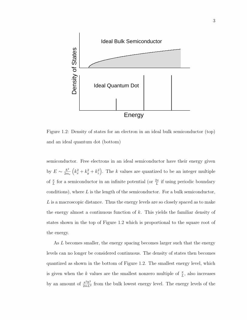
Figure 1.2: Density of states for an electron in an ideal bulk semiconductor (top)

and an ideal quantum dot (bottom)

semiconductor. Free electrons in an ideal semiconductor have their energy given

by E ∼ h2

2me

(k2

x + k2y + k2

z

). The k values are quantized to be an integer multiple

of πL

for a semiconductor in an infinite potential (or 2πL

if using periodic boundary

conditions), where L is the length of the semiconductor. For a bulk semiconductor,

L is a macroscopic distance. Thus the energy levels are so closely spaced as to make

the energy almost a continuous function of k. This yields the familiar density of

states shown in the top of Figure 1.2 which is proportional to the square root of

the energy.

As L becomes smaller, the energy spacing becomes larger such that the energy

levels can no longer be considered continuous. The density of states then becomes

quantized as shown in the bottom of Figure 1.2. The smallest energy level, which

is given when the k values are the smallest nonzero multiple of πL, also increases

by an amount of π2h2

2mL2 from the bulk lowest energy level. The energy levels of the

4

600 800 1000 1200 1400λ(nm)

0

0.5

1

Abs

orba

nce

Absorbance of 990 nm PbSe QDs

First Exciton Peak at 990 nm

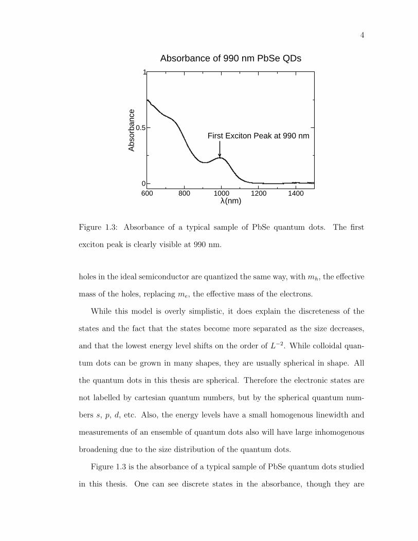
Figure 1.3: Absorbance of a typical sample of PbSe quantum dots. The first

exciton peak is clearly visible at 990 nm.

holes in the ideal semiconductor are quantized the same way, with mh, the effective

mass of the holes, replacing me, the effective mass of the electrons.

While this model is overly simplistic, it does explain the discreteness of the

states and the fact that the states become more separated as the size decreases,

and that the lowest energy level shifts on the order of L−2. While colloidal quan-

tum dots can be grown in many shapes, they are usually spherical in shape. All

the quantum dots in this thesis are spherical. Therefore the electronic states are

not labelled by cartesian quantum numbers, but by the spherical quantum num-

bers s, p, d, etc. Also, the energy levels have a small homogenous linewidth and

measurements of an ensemble of quantum dots also will have large inhomogenous

broadening due to the size distribution of the quantum dots.

Figure 1.3 is the absorbance of a typical sample of PbSe quantum dots studied

in this thesis. One can see discrete states in the absorbance, though they are

5

clearly inhomogenously broadened. The lowest energy level is clearly seen and it is

labeled as the first exciton peak. The first exciton peak is the transition from the

unexcited state of the semiconductor to having one electron in the lowest electron

state, the se state and one hole in the lowest hole state, the sh state. Throughout

this thesis quantum dots will either be denoted by the peak of the luminescence or

the peak of first exciton. For example the plots in later chapters that just denote

PbS quantum dots with 770 nm absorbance, imply that the quantum dots have

its first exciton peak at 770 nm. It will of course have a very broad absorption.

Much more realistic treatments require knowledge of the actual band struc-

ture of the semiconductor. Therefore, while the semiconductor quantum dots will

all roughly have the general characteristics described above, the actual electronic

structure will differ between each semiconductor. When dealing with the actual

electronic structure, semiconductor quantum dots are separated into three confine-

ment regimes.

In the weak confinement regime the size of the quantum dot is larger than

both the Bohr radius of the electron and the hole. The exciton created in this

type of quantum dot acts much like an exciton in the bulk. In the intermediate

confinement regime, only the electron is confined. When both the electron and

hole are confined, both the electron and hole have their energy levels increased

and quantized. This is referred to as strong confinement. Semiconductor quan-

tum dots with strong confinement exhibit the greatest enhancement in optical

properties. Whether a semiconductor system can exhibit intermediate or strong

confinement depends mainly on the properties of the bulk semiconductor, as the

smallest quantum dot that can be grown is still a few lattice constants in size. In

some semiconductors the Bohr radius for the electron or hole will be too small to

6

be confined in a quantum dot that can be realistically grown.

Quantum dots have many useful optical qualities. Because the states are quan-

tized, the dipole strengths are greatly increased from the bulk. Also, as long as

the surface of the quantum dot is well passivated such that there are no traps for

either electrons or holes, the quantum yield should be higher than in the bulk, as

the electron and hole can not drift away from each other as in the bulk.

Though the energy levels are quantized, there is still many of them. This gives

quantum dots a characteristically broad absorption. The quantum dots studied in

this dissertation all relax to the lowest energy state before emitting. This gives

them a characteristically narrow emission. While a broad absorption and nar-

row emission is similar to the bulk semiconductor, this property is quite different

from usual fluorophores such as dyes, As quantum dots are often compared with

fluorophores such as dyes, it is important to note the difference.

Since the lowest energy level is determined by the confinement, the emission

wavelength can be tuned by the size. This allows for semiconductor nanocrystals,

all of which have the same chemical composition, to span a wavelength range. The

long wavelength is determined by the bandgap of the bulk, though there is no

enhancement for dots that are this size. The short wavelength is determined by

the size necessary to make a crystal lattice, usually 1-2 nm[1].

There are many semiconductor systems that can be made into colloidal quan-

tum dots. In this thesis we will look at two different wavelength regions. The

visible, which is useful for biological imaging, is covered by the CdSe quantum

dots. The CdSe quantum dots however only have intermediate confinement. Only

the electron is confined by the size. The hole is unaffected. It is common for the

CdSe quantum dots to have a ZnS cap to improve the quantum yield because of

7

better surface passivation from the ZnS as opposed to the ligands.

The PbS and PbSe dots span the near-infrared which is the useful range for

telecommunications. Both the PbS and PbSe quantum dots are strongly confined.

While PbSe can have a higher band gap semiconductor cap[8], in this work the

PbS and PbSe quantum dots without a cap are used.

1.2 Organization of the Dissertation

This dissertation is divided roughly into two parts. The first discusses research

done with the CdSe/ZnS quantum dots. This part will include a quick intro-

duction along with attempts to put the quantum dots inside cell membranes and

model membrane systems in chapter two. Chapter three will include a part on the

encapsulation of the quantum dots with sphingosine in an attempt to detect phos-

phorylation of the sphingosine. The final chapter on CdSe/ZnS quantum dots,

chapter four, will discuss a final attempt at membrane potential detection and

conclude the work with CdSe/ZnS.

The second part discusses the research done with the lead salt, PbS and PbSe,

quantum dots. The fifth chapter will pertain to measuring the nonlinearity of the

lead salts. After that the lifetime of PbS quantum dots will be discussed and the

implications for the dielectric screening model will be covered. Then fluorescence

resonant energy transfer between the PbS quantum dots will be covered last of

all.

CHAPTER 2

CDSE/ZNS QUANTUM DOTS IN BIOLOGY

2.1 Introduction

CdSe has a bulk bandgap of 730 nm[9]. Quantum confinement can make the first

resonance from the bulk all the way down to 400 nm [1][10][11]. This makes

them useful as fluorophores for biological imaging [12][13][14]. As mentioned in

the introduction, the CdSe quantum dots do not exhibit strong confinement. Only

the electrons are confined by the quantum dot, not the holes. CdSe quantum dots

usually have a capping layer of ZnS. The ZnS passivates the surface better than

the ligand, and thus it increases the quantum yield. A diagram of a CdSe quantum

dot is in Figure 2.1.

CdSe/ZnS quantum dots have the characteristic narrow emission and broad

excitation of semiconductor nanocrystals. For comparison, in Figure 2.2 the exci-

tation and emission of green emitting CdSe/ZnS quantum dots is compared with

a standard dye, Rhodamine B. This fact, coupled with the fact that the emission

wavelength is tunable by size without changing the chemical makeup of the surface

or dot, make them ideal for multicolor imaging[15]. They have also been shown to

exhibit a large Stark shift[16][17][18][19].

To use quantum dots in biological applications, they have to be made water-

soluble. As made, the quantum dots are covered in a hydrophobic ligand, usually

trioctylphosphine oxide (TOPO). This ligand is used in the growth process and al-

lows the quantum dot to be soluble in nonpolar organic solvents. Early on, making

the quantum dots water-soluble proved to be quite difficult. When this research

was started, this problem was just being solved. Quantum dots can be made

8

9

O P

O P

O P

OP

OP

OP

OP

O

P

O

P

OP

OP

OP

OP

OP

OP

OP

OP

OP

OP

OP

O

P

O

P

OP

OP

OP

OP

CdSe

ZnS

TOPO

Figure 2.1: Diagram of a CdSe/ZnS quantum dot

water-soluble by coating them in silica coat[12], exchanging the TOPO molecule

for a water-soluble ligand[13][4], or encapsulating the TOPO covered dot with an

amphilic polymer[20] or lipid[14]. The water-solubility issue is now considered

solved. Water-soluble CdSe/ZnS quantum dots are now commercially available.

Nonetheless, both organic-soluble quantum dots and water-soluble quantum dots

were studied. The quantum dots used in this chapter were provided by Marcel

Bruchez of Quantum Dot Corporation of Hayward, California.

2.2 Initial Characterization

Before research began into using the quantum dots as voltage sensors, an initial

characterization of the dots was performed. The CdSe/ZnS quantum dots have

been known to be bright fluorescent biological labels[12][13]. Unfortunately, they

were also known to blink[21]. Their fluorescence would turn on and off randomly

when excited. This property is undesireable especially in potential applications

that require single molecule tracking. These qualities of the quantum dot were

10

200 300 400 500 600 700Wavelength (nm)

0

0.2

0.4

0.6

0.8

1EmissionExcitation

Rhodamine B

200 300 400 500 600Wavelength (nm)

0.2

0.4

0.6

0.8

1

Excitation (detected at 533 nm)Emission (excited at 350 nm)

CdSe/ZnS Quantum Dots

Figure 2.2: Top: CdSe/ZnS Photoluminscence Excitation and Emission; Bottom:

Rhodamine B Photoluminscence Excitation and Emission for comparison

11

desired to be characterized with fluorescence correlation spectroscopy (FCS). As

this initial characterization is already well reported in publication[22] and Dan

Larson’s thesis[23], only a summary of the results will be given here. Both the

organic-soluble and water-soluble dots were used in this study. The quantum dots

were made water-soluble by coating the dot with an amphilic polymer as described

in Reference [20].

FCS is a relatively straightforward experiment. A recent review of FCS is

given in Reference [24]. An optical focal volume of less than a femtoliter is setup

inside a solution containing the fluorophores. The fluorophores diffuse into and

out of the focal volume by Brownian motion. The experiment is setup such that

only fluorophores that are in the focal volume are both excited and have their

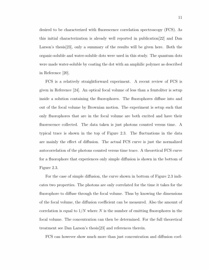
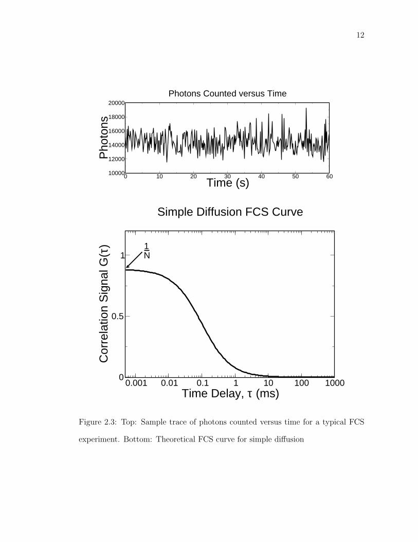
fluorescence collected. The data taken is just photons counted versus time. A

typical trace is shown in the top of Figure 2.3. The fluctuations in the data

are mainly the effect of diffusion. The actual FCS curve is just the normalized

autocorrelation of the photons counted versus time trace. A theoretical FCS curve

for a fluorophore that experiences only simple diffusion is shown in the bottom of

Figure 2.3.

For the case of simple diffusion, the curve shown in bottom of Figure 2.3 indi-

cates two properties. The photons are only correlated for the time it takes for the

fluorophore to diffuse through the focal volume. Thus by knowing the dimensions

of the focal volume, the diffusion coefficient can be measured. Also the amount of

correlation is equal to 1/N where N is the number of emitting fluorophores in the

focal volume. The concentration can then be determined. For the full theoretical

treatment see Dan Larson’s thesis[23] and references therein.

FCS can however show much more than just concentration and diffusion coef-

12

0 10 20 30 40 50 60Time (s)

10000

12000

14000

16000

18000

20000P

hoto

nsPhotons Counted versus Time

0.001 0.01 0.1 1 10 100 1000Time Delay, τ (ms)

0

0.5

1

Cor

rela

tion

Sig

nal G

(τ)

Simple Diffusion FCS Curve

1N

Figure 2.3: Top: Sample trace of photons counted versus time for a typical FCS

experiment. Bottom: Theoretical FCS curve for simple diffusion

13

ficients. Processes that affect the fluorescence of the particle that happen on time

scales smaller than the diffusion time scale can also be seen. Blinking, such as a

dye going into a non-emitting triplet state, can be seen if the blinking time (the

triplet lifetime in this case) is less than the diffusion time. This is because amount

of correlation, 1/N , is the number of emitting fluorophores. If the fluorophores can

go from a nonemitting state to an emitting state on a time scale smaller than dif-

fusion, then the amount of correlation will show that change. Photobleaching can

be seen as an excitation intensity dependent change in the apparent diffusion time.

There is no correlation between photons after a fluorophore has been bleached as

well as when it diffuses out of the focal volume.

If the solution being studied is made of more than one fluorophore, each with

greatly different diffusion coefficients, FCS will also be able to show this. This

was not an issue with this study of quantum dots, as the quantum dots did not

aggregate and were quite monodisperse. In the next chapter of this thesis, however,

single quantum dots will be encapsulated in lipid micelles to make them water

soluble. FCS serves as a great diagnostic in that case, as it can easily determine if

the micelle encapsulates just one quantum dot or many.

The FCS experiment provided significant insight into the quantum dots. FCS

of the quantum dots showed an apparent concentration increase versus excitation

intensity. This was explained as an saturation of absorption which made the di-

mensions of the focal volume effectively increase with excitation intensity. Equally

important is that FCS measured the diffusion of the quantum dots. The diffusion

measurements showed that the quantum dots had a much larger hydrodynamic ra-

dius than expected. In other words, quantum dots diffuse slower than hard spheres

of the same size. Quantum dots soluble in nonpolar organic solvents that were only

14

5 nm in diameter have a 9 nm hydrodynamic radius. For water-soluble dots which

have an amphilic polymer layer over the TOPO ligands[20], the hydrodynamic

radius was 14 nm.

The hydrodynamic radius is significant, not that the radius represents an actual

size, but that attaching the dots to biological molecules will affect their movement

more than previously thought. It is also of note that the larger than expected

hydrodynamic radius had been mentioned in an early study by Mattoussi and

coworkers [25].

FCS also showed no blinking on the millisecond (diffusion) timescale in solution.

However, later research by others[26] indicated that conclusion to be incorrect.

The dots still blink even in solution. The reason for the different conclusion as

explained by the researchers was that the autocorrelation function would not be

able to distinguish the blinking of quantum dots because the blinking has a power-

law distribution[27].

2.3 Membrane Potential Measurements

There is a desire in neuroscience to be able to do real-time imaging of electrical

signaling in cellular systems such as neurons. To do so, fluorophores are required

that are bright, photostable, nontoxic, and have a large, fast change in fluorescence

in the presence of an electric field. A typical membrane is 4 nm across with a

maximum voltage of 100 mV. This means that the fluorophore must be able to

have a measurable change in signal at 250 kV/cm. The change should also take

place in less than 1 ms. Voltage sensing fluorophores usually fall into two categories.

One relies on molecular reorientation or redistribution in the presence of an electric

field. This is slow process, but often produces very large shifts in fluorescence[28].

15

QD

Figure 2.4: Schematic of a quantum dot inside a lipid bilayer. Figure roughly to

scale.

The other rely on an electrochromic effect that is fast, but often not very large[29].

2.4 Stark Effect Measurements

Earlier studies by Colvin and coworkers [16][17][18] and Empedocles and coworkers

[19] indicated that the quantum dots have a large Stark Effect. The Empedocles

study measured a quadratic luminescence shift for single CdSe/ZnS the order of 40

meV at 250 kV/cm. This study was with single dots on a glass slide at 10 K. Also

of note, Empedocles and coworkers measured this shift for CdSe dots with a ZnS

capping layer. One may have thought that the ZnS capping layer would provide

some screening of the electric field and that was not the case.

Given the large measured Stark shift of the quantum dots, the purpose of our

study was to see if the quantum dots could detect changes in cellular membrane

potential. This required the solution to two distinct problems. First was whether

or not quantum dots could be put inside membranes. A typical membrane is only

4 nm thick, while a typical dot is around 5 nm in diameter not including the

16

ligands. Figure 2.4 shows a diagram of the relative sizes of a quantum dot and

a lipid bilayer. Needless to say, a quantum dot will greatly perturb a biological

membrane.

The next question is whether the dots would still be sensitive to voltage changes.

The roughly 250 kV/cm maximum field across a membrane is based on the roughly

100 mV potential over 4 nm. With the membrane perturbed to be almost 10 nm

thick with the dot, a reduction of 2.5 can be reasonably expected in field. Also,

since the dots have to be modified to make them water soluble, there is a question

of whether that will cause screening effects.

2.5 Black Lipid Membranes

The first attempt to study these problems were with black lipid membranes (BLM)

[30]. Black lipid membranes are simple model membrane systems that are sus-

pended over a hole in a plastic sheet in salt water. Electrodes can be put in the

salt water on both sides of the membrane, and thus control the voltage across the

membrane. This system should allow the study of quantum dots in a bilayer.

The method is as follows. Egg Phosphatydilcholine acquired from Avanti Polar

Lipids was dissolved in decane. The plastic support was made of a thin peice

of polyethylene. A hole was made in the center by use of a hot (>100 C) needle

brought close, but without touching the plastic. The hot needle was removed when

the hole was just less than 1 mm in diameter as seen by eye. Then the plastic

support was immersed in salt water. The lipid decane mixture was “painted” or

spread over the hole. The lipid mixture then begins to thin to a bilayer.

Since quantum dots in their usual form are soluble in nonpolar organic solvents

such as decane, it was hoped that by putting the quantum dots in the lipid-

17

decane mixture would protect them from the water. Water-soluble quantum dots

can’t be used, because they are surrounded by hydrophilic molecules, and would

immediately leave the bilayer. Quantum dots soluble in nonpolar organic solvents

can’t be put into the water after the BLM has thinned because the dots are very

hydrophobic and will immediately aggregate.

The end result, however, was that the lipid-decane-QD mixture when “painted”

over the hole in the plastic would not thin to a bilayer. Thus no membrane potential

experiment could be done. This work was done with the help of Professor Peter

Hinkle from the Molecular Biology and Genetics department at Cornell University.

2.6 Giant Unilamellar Vesicles

In the hopes that another model membrane system would work, the membrane

system of giant unilamellar vesicles was tried. A unilamellar vesicle is a single

lipid bilayer that has formed the shape of a sphere. The giant refers to it being

greater than 10 µm. The purpose was to try an experiment similar to that done

by Jerome Mertz and coworkers[31]. This involves putting a GUV between two

electrodes. An AC field is put between the electrodes and due to the mobility of

ions inside the GUV near the bilayer, a field is produced on certain parts of the

GUV. This is a much more complex experiment than the BLM.

GUVs were formed using either the method of electroswelling[32] or by the

method of hydration after evaporation[33]. The electroswelling method requires

drying lipids out in chloroform on large sheets of indium tin oxide (ITO). Then

placing the sheets of ITO together space about 1 mm apart and filling the area

with 50 mM sucrose solution. Then an AC field of 2 V at 5 Hz is applied for 2 hours

and the GUVs form. The other method merely requires lipids to be evaporated

18

in a Teflon or glass tube. Then they are slowly hydrated in a humid incubator at

37 C. The electroswelling method produced better vesicles in terms of uniformity.

The same issue of whether to use quantum dots that are soluble in nonpolar

organic solvents or water-soluble quantum dots is considered. Again since lipids

and quantum dots both dissolve in organic solvents, the method tried was to dis-

solve the quantum dots and lipids together in chloroform. The chloroform mixture

was then evaporated onto the ITO plates. The rest of the procedure was then

followed to try to form the GUVs. Unfortunately, while GUVs would form, none

of the quantum dots would be inside the bilayer of the GUVs. Because of this, the

experiment similar to Reference [31] was never setup or tried. This work was done

with the help of Tobias Baumgart of the Webb group.

2.7 Rat Basophilic Leukemia Cells and Gramicidin

Another attempt was made but now using an already stable cellular system. The

Rat Basophilic Leukemia (RBL) cells are a standard model cell that is easily grown

in Webb group lab. Upon introduction of gramicidin to RBL cells, their usually

large negative membrane potential quickly reduces to zero[34][35].

RBL cells were grown on thin plastic sheets in the Webb lab. After switching

the cells from a growth medium to Tyrodes buffer with glucose, the sheets were then

cut and put into a cuvette. The cuvette was placed in the sample compartment of a

PTI fluorometer, and the fluorescence was monitored. The dye used in References

[34][35], bisoxonol, was tried first. Bisoxonol easily goes into the RBL membrane

after it is introduced into water. Unlike an organic-soluble quantum dot, it is

only slightly hydrophobic. Upon introduction of gramicidin to the RBL cells, the

fluorescence of the bisoxonol greatly increased as expected.

19

The water-soluble dots were used this time, as there was no way to get the

organic-soluble quantum dots into the RBL cells without them aggregating. While

it was realized that the water-soluble dots would not go into the membrane, it was

hoped that some would stick to the membrane and be close enough to be affected

by the electric field. This was not the case, the quantum dots had no affinity

towards the cells.

2.8 Conclusion

The end result was that none of these methods worked. The model membrane

systems of the giant unilamellar vesicles and black lipid membranes would not

form with quantum dots in them. The RBL cells were very difficult to get quantum

dots to stick to, and they did not show any sign of a fluorescence change with the

addition of gramicidin. Possible reasons for this failure will be discussed in a later

chapter.

CHAPTER 3

CDSE/ZNS QUANTUM DOTS FOR STUDIES OF SPHINGOLIPID

METABOLISM

3.1 Sphingolipid Metabolism

With the membrane potential measurements providing no results, a new idea was

set forth by professor David Russell of the Microbiology and Immunology depart-

ment of the College of Veterinary Medicine at Cornell. His idea was to encapsulate

quantum dots not in a bilayer, but in a spherical micelle. Then by changing the

charge on lipids encapsulating the quantum dot, perhaps the quantum dot would

have its luminescence shift due to the change in electric field. Around the same

time a research paper was published by a Dubertret and coworkers at Rockefeller

University, that successfully encapsulated quantum dots in a spherical micelle with

a mixture of lipids to make the quantum dots water-soluble[14].

The lipids to be studied in this research were the sphingolipids. The sphin-

golipids are an important class of lipids involved in the signal transduction path-

ways that mediate cell growth, differentation, and death. Sphingosine is the most

common backbone of the sphingolipids, and the phosphorylation of sphingosine is

an important step in sphingolipid metabolism[36].

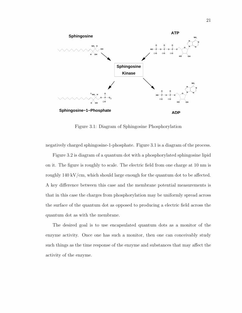
The specific process that is desired to be studied is the phosphorylation of

sphingosine into sphingosine-1-phosphate. Phosphorylation is the addition of a

charged phosphate group to a lipid. The phosphorylation of sphingosine requires

the enzyme sphingosine kinase and adenosine triphosphate (ATP). The enzyme

takes a phosphate group from the ATP and attaches it to the sphingosine. The

ATP becomes adenosine diphosphate (ADP) and the sphingosine becomes the

20

21

OH

OH

NH 2

H

H

Sphingosine

O P O

O

O

H P O

O

O

P O

O

O

HO

O

HO

N

N

NH2

N

N

ATP

Sphingosine

Kinase

O P O

O

O

NH 3 H

OHH

Sphingosine−1−Phosphate

P O

O

O

O P O

O

O

H

HO

O

HO

N

N

NH2

N

N

ADP

Figure 3.1: Diagram of Sphingosine Phosphorylation

negatively charged sphingosine-1-phosphate. Figure 3.1 is a diagram of the process.

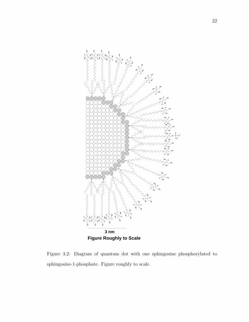
Figure 3.2 is diagram of a quantum dot with a phosphorylated sphingosine lipid

on it. The figure is roughly to scale. The electric field from one charge at 10 nm is

roughly 140 kV/cm, which should large enough for the quantum dot to be affected.

A key difference between this case and the membrane potential measurements is

that in this case the charges from phosphorylation may be uniformly spread across

the surface of the quantum dot as opposed to producing a electric field across the

quantum dot as with the membrane.

The desired goal is to use encapsulated quantum dots as a monitor of the

enzyme activity. Once one has such a monitor, then one can conceivably study

such things as the time response of the enzyme and substances that may affect the

activity of the enzyme.

22

OH

OH

2H

NH

H

3 nm

Figure Roughly to Scale

O P

O P

O P

OP

OP

OP

OP

O

P

O

P

OP

OP

OP

OP

H 3N H

OHH

O O

O

P

O

OH

OH

2HN

H

H

OH

OH

2HN

H

H

OH

OH

2HN

H

H

OH

OH

2H

N H

H

OH

OH

2H

N H

H

OH

OH

2H

N H

H

OH

OH

2HN

H

H

OH

OH

2HN

H

H

OH

OH

2HN

H

H

OH

OH

2HN

H

H

OH

OH

2HN

H

H

OHOH

2HN

HH

OH

OH

2H

N

H

H

OH

OH

2H

NH

H

OH

OH

2H

NH

H

OH

OH

2H

N

H

H

OH

OH

2H

NH

H

OH

OH

2H

N

H H

OHOH

2HN

H

H

OH

OH

2HN

H

H

OHOH

2HN

H

H

OH

OH

2HN

H

H

OH

OH

2H

N

H

H

OH

OH

2H

N H

H

OH

OH2

HN

H

H

Figure 3.2: Diagram of quantum dot with one sphingosine phosphorylated to

sphingosine-1-phosphate. Figure roughly to scale.

23

3.2 Encapsulating Quantum Dots with Sphingosine

Dubertret and coworkers were able to encapsulate quantum dots in a mixture

of dipalmitoyl phosphatidylethanolamine-polyethylene glycol (DPPE-PEG) and

dipalmitolyphosphatidylcholine (DPPC). Both DPPE-PEG and DPPC are lipids

with fully saturated double hydrocarbon chains of 16 unit length. While they

tried several different lipid combinations, they concluded that both the PEG and

a double hydrocarbon chain found on the DPPE were needed. However, a lot is

known about the self-assembly of lipids[37][38][39], and using that knowledge one

should be able to change the method of Dubertret and coworkers to use sphingosine.

There are three characteristics a lipid must have to form a micelle[37][38][39].

The first is that the lipid must be amphilic, which means it must have both a

hydrophilic part, the polar headgroup, and a hydrophobic part, the hydrocarbon

chain. Since there is no chemical bond between the hydrocarbon chains, the hy-

drophobic part must be large enough to make the structure stable. Technically,

this means the lipid must have a low critical micelle concentration (CMC). The

CMC is the concentration at which the lipids will start to self-assemble into struc-

tures. If the concentration is below the CMC, the lipids will just exist separately

in solution.

The CMC is given generally by the equation CMC≈ exp[−(µ01 − µ0

N)/kBT ].

The factor kBT is Boltzmann’s constant multiplied by the temperature. The con-

stant µ01 is the standard part of the chemical potential or the mean interaction

free energy per molecule for single molecules in solution. Likewise µ0N is for the

aggregate of molecules, in this case a micelle. N is just the number of molecules

in the aggregate[37]. Unlike the difference between the chemical potentials, the

CMC is easily measured. Thus the discussion will use the CMC as the measure

24

of stability or affinity between the lipids, though there is no real chemical bond

or attractive force. The lower the CMC, the greater the difference between the

chemical potentials of the single molecule with respect to the micelle. This then

implies greater stability of the micelle structure.

The CMC of an amphilic molecule depends on the size of hydrophobic hydro-

carbon chains with respect to the size of the hydrophilic part. Lipids usually have

either one or two hydrocarbon chains. Those with two hydrocarbon chains have a

much lower CMC. Also by increasing the length of the chain, the CMC goes down

as well. For some typical numbers, a phosphatidylcholine (PC) with a double 5

unit hydrocarbon chain has a CMC of 90 mM. One with a double 10 unit chain

has a CMC of .005 mM. And a PC with just a single 10 unit chain has a CMC of

8 mM[40].

The second characteristic needed is that the lipid must also have the proper

packing geometry to form a micelle as opposed to other structures, such as the more

common bilayer. The measure used here is the critical packing parameter (CPP).

The CPP of a amphilic molecule is defined as the volume (v) of the hydrocarbon

chains divided by the product of the area of the head group (a) and the length of

the hydrocarbon chain (l), or CPP= v/al. For a micelle to form, the CPP must be

at or below one third. This can be seen by just dividing the volume of a sphere by

its surface area and radius. For a bilayer, the CPP must be around one. Thus the

CPP is a measure of the curvature of the structure the amphilic molecule will form.

For example, if one wanted to encapsulate a sphere of diameter 5 nm with lipids

of hydrocarbon length 2 nm, the volume of the hydrocarbon chains would have to

be v = 43π((2.5 + 2)3 − 2.53). The surface area would have to be a = 4π(2.5 + 2)2.

This would require a molecule with a CPP of 0.62.

25

The last characteristic is that there must be some sort of repulsive interaction to

keep the encapsulated dots from aggregating. It is important to note however that

the actual self-assembly dynamics are much more complex. This simple version

neglects several important properties. The phase transition temperature of the

lipids is an important property that is neglected. This affects the volume of the

hydrocarbon chains. The effect of salt and pH on the lipids is also important. Salt

can screen charges on the headgroups of the lipids which will decrease the surface

area of the head groups. Also changes in pH can actually change the charge on

the head groups as well. Also since the hydrocarbon chains aren’t rigid, the CPP

is not really an exact requirement. It is more of a guideline. However, this simple

version of self-assembly dynamics is more than good enough to provide a starting

point in picking lipids and rules of thumb in deciding how to adjust the procedure.

Often however, it is difficult to have all the necessary characteristics to form

micelles with low CMCs met at the same time. For instance DPPC, which is one

of the shorter chain length components of GUVs, BLMs, and cellular membranes,

has a very low CMC, 4.6× 10−10M [40]. This fact makes cellular membranes very

stable. Unfortunately, its geometry is such that it forms bilayers. Not surprisingly,

Dubertret and coworkers were unable to form micelles with DPPC alone. Usually

lipids that form micelles usually have either very short double hydrocarbon chains

or short single hydrocarbon chains, and therefore they usually have CMCs in the

millimolar range. DPPE-PEG is an exception as it has a long double hydrocarbon

chains that give it a CMC of 70 µM[41]. A mixture of DPPC and DPPE-PEG

will lower the CMC still, though it will increase the overall average CPP. As

previously calculated, the CPP for encapsulating a quantum dot (∼0.6) is more

than is required for a micelle (∼0.33), so the addition of DPPC should be beneficial.

26

The DPPE-PEG lipid also has the steric hindrance from the PEG. This keeps not

only biomolecules from sticking to the quantum dots, but also keeps the quantum

dots from sticking to each other.

When trying to encapsulate dots with sphingosine, different lipids were tried

besides DPPE-PEG. It was feared that the steric hindrance of the PEG might

interfere with the enzyme. That concern coupled with an initial difficulty in getting

the DPPE-PEG/DPPC encapsulation to work, caused other lipids to be tried

first. As seen in Figure 3.1 sphingosine has no real head group and is therefore

very hydrophobic. The quantum dots are covered with trioctylphosphine oxide

(TOPO), which is also very hydrophobic. TOPO has a triple hydrocarbon chain,

with each chain is 8 units long. Trying to encapsulate quantum dots in sphingosine

alone doesn’t work. The sphingosine and quantum dots just clump together and

aggregate out of solution. Therefore a mixture of lipids is required.

It is known that 12 unit single chain PC forms micelles[42] as well as 7 unit

double chain PC[43]. These would be the limit the lower end of the chain length,

as they have high CMCs and low CPPs. Due to price considerations, not all

lipid combinations can be tried and the PC lipids are often the cheapest. Since

the CPP of the encapsulating lipids should be higher than required for micelle

formation, slightly longer lipids can be used to lower the CMC. As for a repulsive

interaction, adding a small amount of charged lipids will keep the quantum dots

from aggregating. The charged lipids choosen where the phosphatic acid (PA)

lipids which are similar to the PC except they are missing the choline group (the

nitrogen and hydrocarbons) attached to the phosphate group making it negative,

and ethylphosphatidylcholine (EPC) which is PC with the phosphate neutralized

making it a positive lipid.

27

O

O

N PO

O

O

O

H

O

O

EDLPC

O

O

OH P

O

O

O

H

O

O

DLPA

O

O

N PO

O

O

O

H

O

O

EDLPC

O P O

O

O

NH 3 H

OHH

Sphingosine−1−Phosphate

OH

OH

NH 2

H

H

Sphingosine

OH

ON

H

PO O

O

O

O

LMPC

Figure 3.3: Chemical structure of the lipids used to encapsulate the quantum dots.

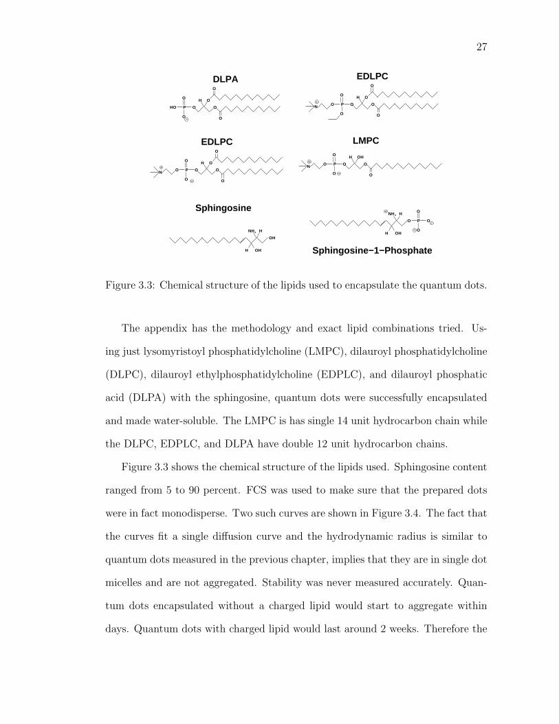
The appendix has the methodology and exact lipid combinations tried. Us-

ing just lysomyristoyl phosphatidylcholine (LMPC), dilauroyl phosphatidylcholine

(DLPC), dilauroyl ethylphosphatidylcholine (EDPLC), and dilauroyl phosphatic

acid (DLPA) with the sphingosine, quantum dots were successfully encapsulated

and made water-soluble. The LMPC is has single 14 unit hydrocarbon chain while

the DLPC, EDPLC, and DLPA have double 12 unit hydrocarbon chains.

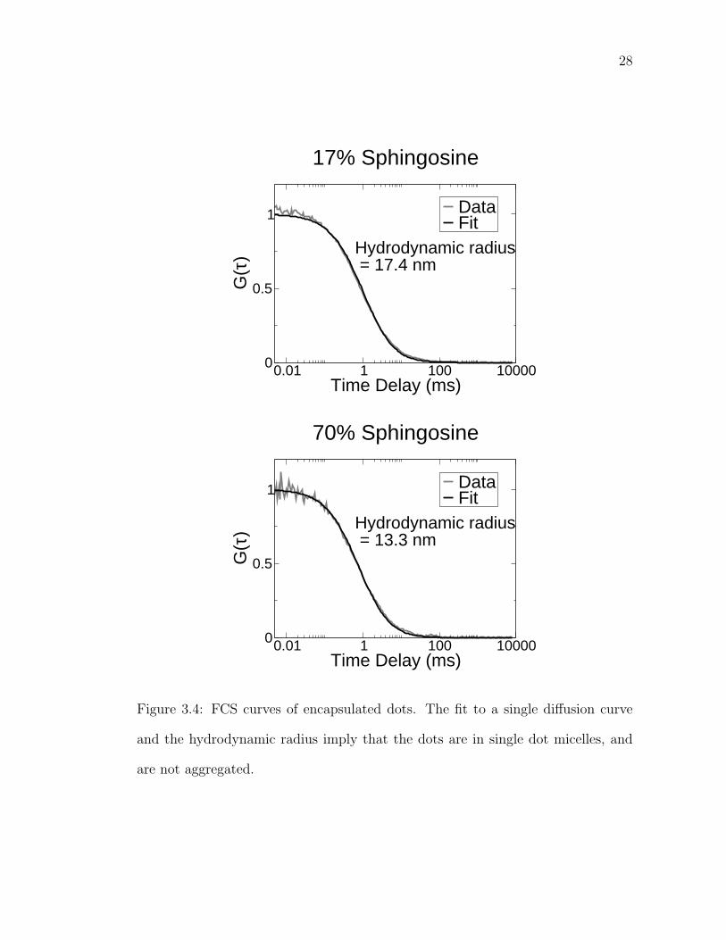
Figure 3.3 shows the chemical structure of the lipids used. Sphingosine content

ranged from 5 to 90 percent. FCS was used to make sure that the prepared dots

were in fact monodisperse. Two such curves are shown in Figure 3.4. The fact that

the curves fit a single diffusion curve and the hydrodynamic radius is similar to

quantum dots measured in the previous chapter, implies that they are in single dot

micelles and are not aggregated. Stability was never measured accurately. Quan-

tum dots encapsulated without a charged lipid would start to aggregate within

days. Quantum dots with charged lipid would last around 2 weeks. Therefore the

28

0.01 1 100 10000Time Delay (ms)

0

0.5

1

G(τ

) Hydrodynamic radius = 17.4 nm

DataFit

17% Sphingosine

0.01 1 100 10000Time Delay (ms)

0

0.5

1

G(τ

) Hydrodynamic radius = 13.3 nm

DataFit

70% Sphingosine

Figure 3.4: FCS curves of encapsulated dots. The fit to a single diffusion curve

and the hydrodynamic radius imply that the dots are in single dot micelles, and

are not aggregated.

29

quality of these dots are inferior to those produced by Dubertret and coworkers.

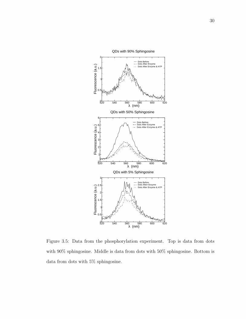
3.3 Sphingosine Phosphorylation Experiments

To test the dots for phosphorylation, the quantum dots were put in a fluorometer

and their luminescence was monitored as enzyme and ATP were added. The

enzyme and ATP were provided by Roisin Owens of David Russell’s lab. The

data are in Figure 3.5. While no shift in fluorescence was seen, the fluorescence

intensity always decreased with ATP and the enzyme being added. Further tests

showed that the fluorescence intensity only decreased when the enzyme was added

whether or not ATP was added at all. The fluorescence was unchanged when just

ATP was added to the dots. Also the fluorescence was decreased less for dots with

a larger percentage of sphingosine on them and for dots with a smaller percentage

of sphingosine on them. Therefore it seems as though the enzyme may be attaching

to the sphingosine, this in turn causes the sphingosine to be more likely to go into

solution and leave the dot. The quantum dot will lose fluorescence yield as it

becomes unprotected.

3.4 Conclusion

After that point, experiments were stopped. It was decided that using the quantum

dots in this way wasn’t easy enough to continue. Russell’s lab which provided

the ATP and enzyme, had other methods to study the enzyme which were much

more likely to produce results. While in the end the experiment didn’t work, it

was an interesting study in self-assembly of lipids around quantum dots. If one

were to try again, serious consideration should be paid to trying to cross-link the

30

520 540 560 580 600 620 λ (nm)

0

0.5

1

1.5

2

Flu

ores

cenc

e (a

.u.)

Dots BeforeDots After EnzymeDots After Enzyme & ATP

QDs with 90% Sphingosine

520 540 560 580 600 620 λ (nm)

0

1

2

3

4

5

6

Flu

ores

cenc

e (a

.u.)

Dots BeforeDots After EnzymeDots After Enzyme & ATP

QDs with 50% Sphingosine

520 540 560 580 600 620 λ (nm)

0

0.5

1

1.5

2

2.5

3

Flu

ores

cenc

e (a

.u.)

Dots BeforeDots Afterr EnzymeDots After Enzyme & ATP

QDs with 5% Sphingosine

Figure 3.5: Data from the phosphorylation experiment. Top is data from dots

with 90% sphingosine. Middle is data from dots with 50% sphingosine. Bottom is

data from dots with 5% sphingosine.

31

lipids so that they don’t come off the quantum dots. This will also improve the

stability. There are many ways to attempt this. There are polymerizable lipids that

upon exposure to ultraviolet light will cross-link[44]. There are also cross-linkable

polymers that can be used, as was done for making carbon nanotubes water-

soluble[45]. The overall mixture would not be fully biological, but that may not

matter. Another avenue to pursue is the phosphorylation and dephosphorylation

of other lipid systems. For instance there is an enzyme that removes the choline

group from PC to make it PA. The issue of whether the quantum dots will feel

the field of charges spread uniformly around its exterior, is another question that

remains to be answered.

CHAPTER 4

CDSE/ZNS QUANTUM DOTS IN BIOLOGY, CONCLUSION

4.1 Revisiting the Membrane Potential Experiments

Due to the work encapsulating the quantum dots with sphingosine, not realizing

the geometry considerations of the lipids while trying to get quantum dots into

membranes was a mistake. Trying to make GUVs and BLMs with the dots in the

lipid solution without altering the composition of the lipids will not work. The

usual procedure to make both GUVs and BLMs require the long double chain

lipids found in egg PC to make stable bilayers. To properly cover a quantum dot,

lipids with a low critical packing parameter (CPP) are required. However, it is not

clear that by altering the GUV or BLM lipid mixture with lower CPP lipids will

allow GUVs or BLMs to form with quantum dots in them. Another structure may

form instead. During the sphingosine experiments, when lipids with too large of a

CPP were used, bilayers with quantum dots in them did not form. What appeared

to be the encapsulation of two or more quantum dots in lipids seemed to be the

result. It just may not be favorable for bilayers to self-assemble around a quantum

dot.

However, if one prepared the bilayer system separately and the encapsulated

quantum dot system separately, one might be able to get the quantum dots into

the bilayer. To get the two together, an idea from drug delivery was borrowed.

Cell membranes are usually negatively charged. There are rarely any naturally

occuring positively charged lipids. A method in drug delivery is that a drug would

be encapsulated in a vesicle that had positively charged lipids[46]. These vesi-

cles would be attracted the cell membrane. They would bind and fuse together,

32

33

emptying the contents of the vesicle into the cell.

The goal then is to encapsulate the quantum dots in lipids, some of which have

a positive charge. The DPPE-PEG/DPPC method was again not used, as the

PEG may interfere with the quantum dot getting to the membrane. In fact water-

soluble quantum dots from Quantum Dot Corporation were not used either. Those

dots, along with most other published methods of making water-soluble dots, are

made expressly to avoid sticking to membranes. They are meant to be attached

to a specific molecule only.

It was not difficult to find a mixture of LMPC, EDLPC, and DLPC that would

work. The EDLPC is a synthetic positively charged lipid. The actual method

is cover in the appendix. It is interesting to note that the addition of a little

(5 percent) sphingosine helped the encapsulation. Without it, there was a 4 nm

redshift in fluorescence and a slight decrease in intensity. That seems to imply

that the lipid mixture is not well optimized and that the sphingosine helps fill in

gaps and lowers the CMC.

4.2 The Aplysia experiment

To test this idea, another voltage sensing experiment was tried. The system used

was Aplysia neurons. Dan Dombeck of Webb group had this system setup, and

was very familiar with it. It is described well in his paper[47]. An Aplysia neuron

is voltage clamped, allowing the voltage across the membrane to be changed. The

system has the sensitivity to detect 1% per 100 mV with averaging. The only

modification of his experiment is the change in detection. His setup detected

changes in second harmonic intensity versus voltage. As the quantum dots are

expected to shift their fluorescence, not change their intensity, that setup wouldn’t

34

20 µm

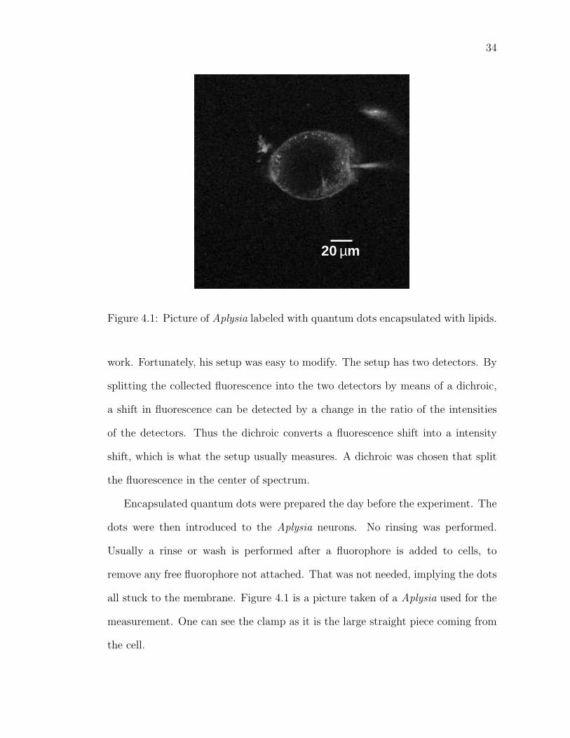
Figure 4.1: Picture of Aplysia labeled with quantum dots encapsulated with lipids.

work. Fortunately, his setup was easy to modify. The setup has two detectors. By

splitting the collected fluorescence into the two detectors by means of a dichroic,

a shift in fluorescence can be detected by a change in the ratio of the intensities

of the detectors. Thus the dichroic converts a fluorescence shift into a intensity

shift, which is what the setup usually measures. A dichroic was chosen that split

the fluorescence in the center of spectrum.

Encapsulated quantum dots were prepared the day before the experiment. The

dots were then introduced to the Aplysia neurons. No rinsing was performed.

Usually a rinse or wash is performed after a fluorophore is added to cells, to

remove any free fluorophore not attached. That was not needed, implying the dots

all stuck to the membrane. Figure 4.1 is a picture taken of a Aplysia used for the

measurement. One can see the clamp as it is the large straight piece coming from

the cell.

35

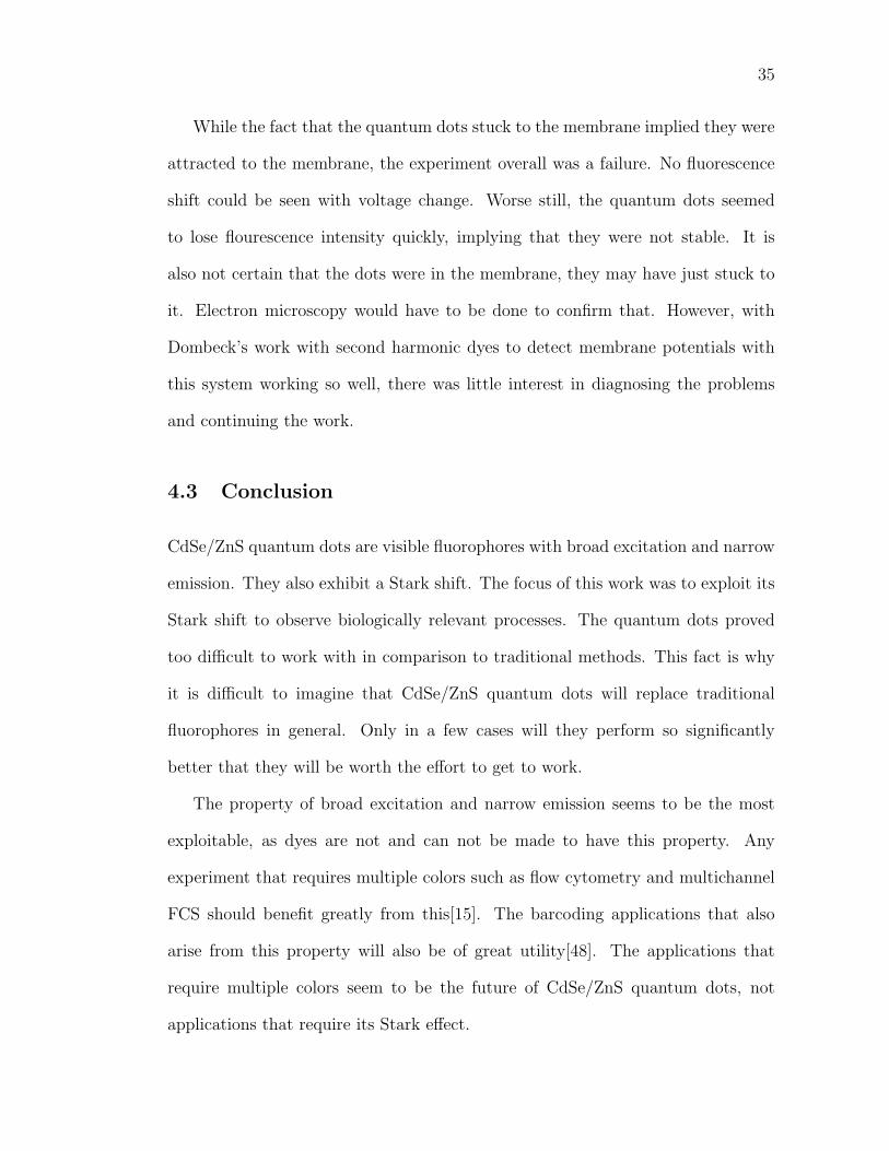
While the fact that the quantum dots stuck to the membrane implied they were

attracted to the membrane, the experiment overall was a failure. No fluorescence

shift could be seen with voltage change. Worse still, the quantum dots seemed

to lose flourescence intensity quickly, implying that they were not stable. It is

also not certain that the dots were in the membrane, they may have just stuck to

it. Electron microscopy would have to be done to confirm that. However, with

Dombeck’s work with second harmonic dyes to detect membrane potentials with

this system working so well, there was little interest in diagnosing the problems

and continuing the work.

4.3 Conclusion

CdSe/ZnS quantum dots are visible fluorophores with broad excitation and narrow

emission. They also exhibit a Stark shift. The focus of this work was to exploit its

Stark shift to observe biologically relevant processes. The quantum dots proved

too difficult to work with in comparison to traditional methods. This fact is why

it is difficult to imagine that CdSe/ZnS quantum dots will replace traditional

fluorophores in general. Only in a few cases will they perform so significantly

better that they will be worth the effort to get to work.

The property of broad excitation and narrow emission seems to be the most

exploitable, as dyes are not and can not be made to have this property. Any

experiment that requires multiple colors such as flow cytometry and multichannel

FCS should benefit greatly from this[15]. The barcoding applications that also

arise from this property will also be of great utility[48]. The applications that

require multiple colors seem to be the future of CdSe/ZnS quantum dots, not

applications that require its Stark effect.

36

If however, someone wished to continue this research there are some ideas to

be pursued. For the sphingosine lipids, the cross-linking lipids or amphilic poly-

mers should be investigated. Also using only core CdSe dots instead of core/shell

CdSe/ZnS dots may prove to be more sensitive. As for the membrane measure-

ments, the idea of first making the dots water soluble separately from the mem-

brane system seems like the correct idea. With that in mind, it is probably wise

to go back to the model membrane systems such as the black lipid membranes.

The BLM system is quite robust and more importantly do not require growing

cell cultures which take a significant amount of time. Cross-linking lipids for the

membrane system may not work, but also could be investigated.

CHAPTER 5

NONLINEAR MEASUREMENTS OF PBSE QUANTUM DOTS

5.1 Introduction

The colloidal lead salt quantum dots are similar to the CdSe quantum dots in that

they have broad excitation and narrow emission. They are different, however, in

that they are strongly confined while the CdSe quantum dots are only intermedi-

ately confined. This is because the Bohr radius of both the electron and holes are

quite large, 10 nm for PbS and 24 nm for PbSe[49].

While PbSe quantum dots have been made with a capping layer (PbSexS1−x)[8],

high quality lead salt quantum dots can be used without a capping layer similar

to ZnS for the CdSe quantum dots. The other major difference is the wavelength

of light at which they emit. The CdSe dots emit in the visible, while the lead salt

quantum dots emit in the near infrared. This is because the band edge for CdSe

is 730 nm while for PbS it is 3 µm and for PbSe it is 4.6 µm [9].

All but the smallest lead salt quantum dots are not useful in biology as water

becomes highly absorptive in the near-infrared. The near-infrared is however, the

wavelength range in which telecommunications are used. The major telecommu-

nications bands are at 1550 nm and 1300 nm. There is a great desire to get good

emitters, detectors, amplifiers, and optical switches in those wavelength ranges.

A general review of the electronic and optical properties of the lead salt quan-

tum dots is given in Reference [50]. More detailed theoretical calculations of the

lead salt quantum dots are given in References [51] and [52].

This study will concentrate on the third-order optical nonlinearity of the lead

salt dots for the potential use of optical switching. Based on data from CdSe

37

38

z

Sample

Detector

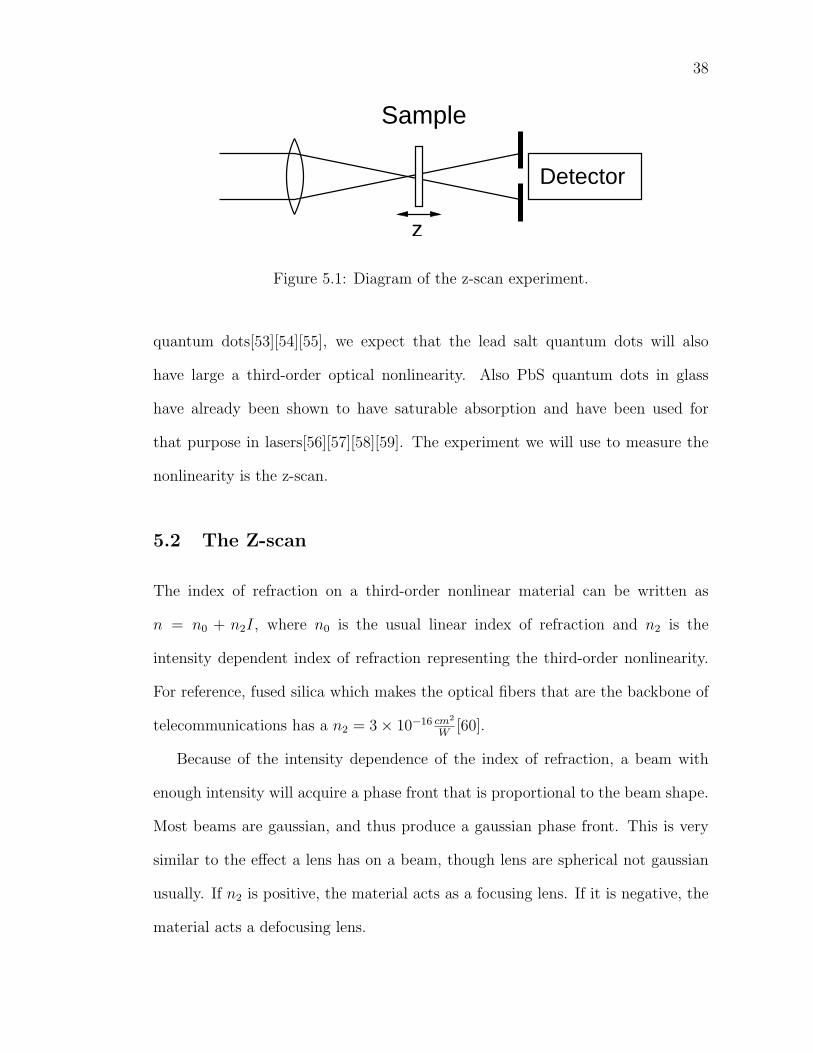
Figure 5.1: Diagram of the z-scan experiment.

quantum dots[53][54][55], we expect that the lead salt quantum dots will also

have large a third-order optical nonlinearity. Also PbS quantum dots in glass

have already been shown to have saturable absorption and have been used for

that purpose in lasers[56][57][58][59]. The experiment we will use to measure the

nonlinearity is the z-scan.

5.2 The Z-scan

The index of refraction on a third-order nonlinear material can be written as

n = n0 + n2I, where n0 is the usual linear index of refraction and n2 is the

intensity dependent index of refraction representing the third-order nonlinearity.

For reference, fused silica which makes the optical fibers that are the backbone of

telecommunications has a n2 = 3× 10−16 cm2

W[60].

Because of the intensity dependence of the index of refraction, a beam with

enough intensity will acquire a phase front that is proportional to the beam shape.

Most beams are gaussian, and thus produce a gaussian phase front. This is very

similar to the effect a lens has on a beam, though lens are spherical not gaussian

usually. If n2 is positive, the material acts as a focusing lens. If it is negative, the

material acts a defocusing lens.

39

-10 -5 0 5 10z/z0

-0.04

-0.02

0

0.02

0.04

∆T/T

Positive n2Negative n2

Theoretical Z-scan Curves

Figure 5.2: Theoretical z-scan curves for both a positive and negative n2.

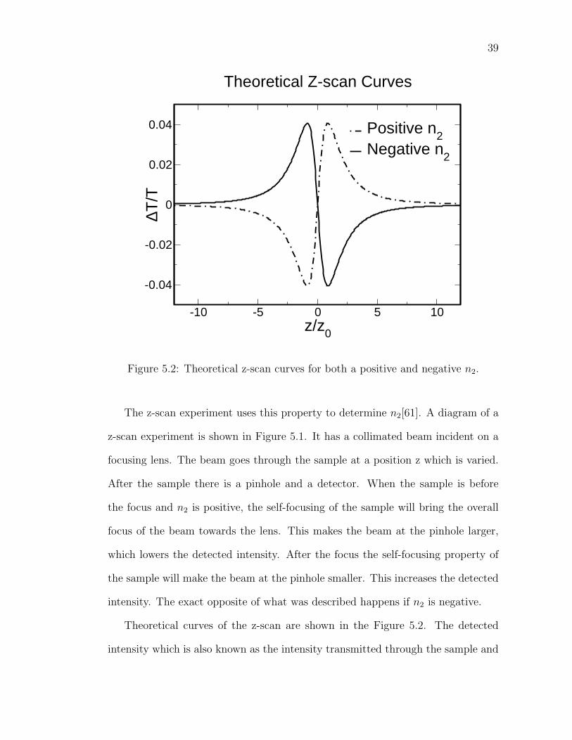
The z-scan experiment uses this property to determine n2[61]. A diagram of a

z-scan experiment is shown in Figure 5.1. It has a collimated beam incident on a

focusing lens. The beam goes through the sample at a position z which is varied.

After the sample there is a pinhole and a detector. When the sample is before

the focus and n2 is positive, the self-focusing of the sample will bring the overall

focus of the beam towards the lens. This makes the beam at the pinhole larger,

which lowers the detected intensity. After the focus the self-focusing property of

the sample will make the beam at the pinhole smaller. This increases the detected

intensity. The exact opposite of what was described happens if n2 is negative.

Theoretical curves of the z-scan are shown in the Figure 5.2. The detected

intensity which is also known as the intensity transmitted through the sample and

40

aperature is denoted as T . The plot shows the normalized change in transmitted

intensity (∆T/T ) versus the z position of the sample. The change, ∆T , is the

difference between detected intensity when the sample is at the current position

z and the detected intensity when it is at a position far from the focus. The

horizontal axis of the plot is normalized to the confocal parameter of the focused

beam, z0.

The z-scan is not a very sensitive way to measure n2. If the sample is non-

uniform, as the sample moves and the beam hitting the sample changes size, the de-

tected intensity will change without the nonlinearity just due to the non-uniformity.

A more sensitive measurement is spectrally-resolved two-beam coupling[62]. This

method works with femtosecond pulses when it is easy to resolve the spectrum

of the laser. Picosecond and longer pulses do not have the bandwidth to easily

spectrally-resolve energy shifts due to the nonlinearity. Long pulses were used in

this study because of the concern that large bandwidth pulses would not be able to

saturate the excited state of the quantum dots. The use of low peak power pulses

also lowers the sensitivity of the experiment.

5.3 The Samples

The samples were provided by Evident Technologies of Troy, New York. They were

provided in films sandwiched between two glass slides. The samples were usually

labeled by their concentration before introduction to the host that comprised the

film. Evident did not give specifics about how the films were made and what exactly

the hosts were made of, so it is difficult to infer much about the quantum dots

themselves. Several samples were given with different first exciton wavelengths.

The most used samples were one with a first exciton wavelength at 1064 nm and

41

500 1000 1500 2000λ (nm)

0

0.2

0.4

0.6

0.8

Abs

orba

nce

Absorbance of 1550 PbSe Sample

Spectra of Laser

Figure 5.3: Absorption of 1550 nm sample and spectra of the laser used for the

measurement.

another at 1550 nm. The quantum dots were put into films that were around 100

µm thick at an intial concentration of 100 mg/mL. The 1064 nm sample was used

with a Nd:YAG Antares that was actively modelocked to produce 100 picosecond

pulses with 200 nJ at 1064 nm. The 1550 nm sample was used with a Coherent

Mira OPO system that produced 1 ps pulses with around 1 nJ of energy at 1550

nm. Both systems produce roughly the same order of magnitude peak power. Since

the 1550 nm sample is at the more relevant wavelength, the rest of the chapter

will deal with that sample. A plot with the absorption of the 1550 nm film and

the spectra of the laser used to measure the sample is shown in Figure 5.3.

42

-5 0 5 10z (mm)

-0.4

-0.2

0

0.2

0.4

0.6

∆T/T

DataFit

Experimental Z-scan Data

Figure 5.4: Sample z-scan data.

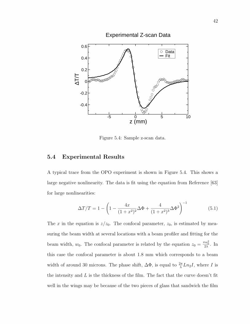
5.4 Experimental Results

A typical trace from the OPO experiment is shown in Figure 5.4. This shows a

large negative nonlinearity. The data is fit using the equation from Reference [63]

for large nonlinearities:

∆T/T = 1−(

1− 4x

(1 + x2)2∆Φ +

4

(1 + x2)3∆Φ2

)−1

(5.1)

The x in the equation is z/z0. The confocal parameter, z0, is estimated by mea-

suring the beam width at several locations with a beam profiler and fitting for the

beam width, w0. The confocal parameter is related by the equation z0 =πw2

0

2λ. In

this case the confocal parameter is about 1.8 mm which corresponds to a beam

width of around 30 microns. The phase shift, ∆Φ, is equal to 2πλ

Ln2I, where I is

the intensity and L is the thickness of the film. The fact that the curve doesn’t fit

well in the wings may be because of the two pieces of glass that sandwich the film

43

of quantum dots.

Unfortunately after careful analysis, this nonlinearity is due solely to thermal

heating effects. Since the quantum dots absorb the laser light, some excess energy

that is not emitted heats the sample. This causes a thermal gradiant that effects

the index of refraction by changes in the density. This was first suspected when the

repetition rate was reduced by an electro-optic modulator. Reducing the repetition

rate reduces the average power incident on the sample by reducing the number of

pulses hitting the sample, but does not change the peak power of the pulses.

Reducing the repetition rate to 1 MHz from the usual 76 MHz caused the signal

to disappear.

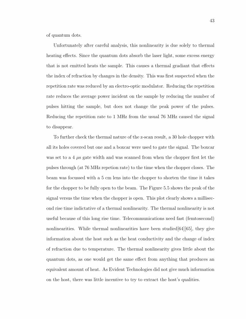
To further check the thermal nature of the z-scan result, a 30 hole chopper with

all its holes covered but one and a boxcar were used to gate the signal. The boxcar

was set to a 4 µs gate width and was scanned from when the chopper first let the

pulses through (at 76 MHz repetion rate) to the time when the chopper closes. The

beam was focussed with a 5 cm lens into the chopper to shorten the time it takes

for the chopper to be fully open to the beam. The Figure 5.5 shows the peak of the

signal versus the time when the chopper is open. This plot clearly shows a millisec-

ond rise time indictative of a thermal nonlinearity. The thermal nonlinearity is not

useful because of this long rise time. Telecommunications need fast (femtosecond)

nonlinearities. While thermal nonlinearities have been studied[64][65], they give

information about the host such as the heat conductivity and the change of index

of refraction due to temperature. The thermal nonlinearity gives little about the

quantum dots, as one would get the same effect from anything that produces an

equivalent amount of heat. As Evident Technologies did not give much information

on the host, there was little incentive to try to extract the host’s qualities.

44

1 10 100 1000Time from start of rise (µs)

0

0.05

0.1

0.15

0.2

∆T/T

peak

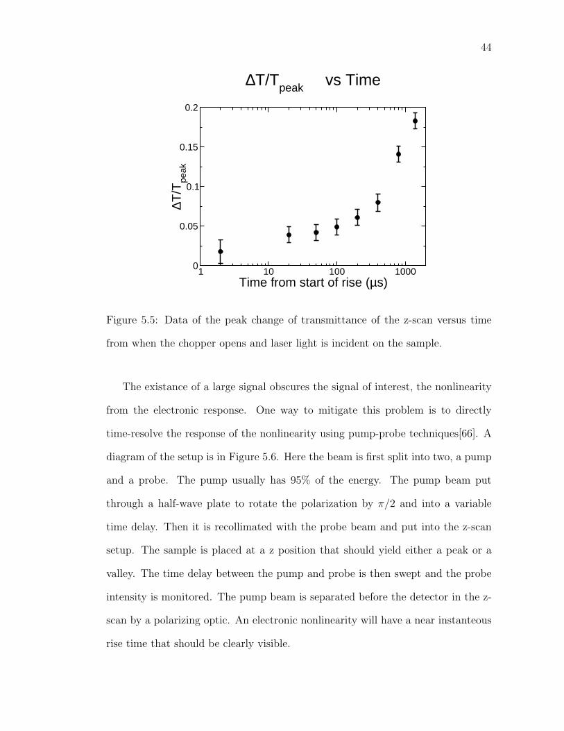
∆T/Tpeak vs Time

Figure 5.5: Data of the peak change of transmittance of the z-scan versus time

from when the chopper opens and laser light is incident on the sample.

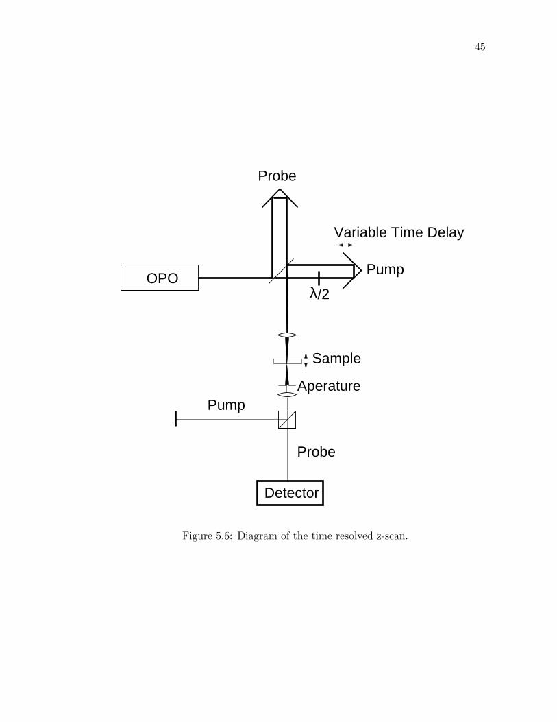
The existance of a large signal obscures the signal of interest, the nonlinearity

from the electronic response. One way to mitigate this problem is to directly

time-resolve the response of the nonlinearity using pump-probe techniques[66]. A

diagram of the setup is in Figure 5.6. Here the beam is first split into two, a pump

and a probe. The pump usually has 95% of the energy. The pump beam put

through a half-wave plate to rotate the polarization by π/2 and into a variable

time delay. Then it is recollimated with the probe beam and put into the z-scan

setup. The sample is placed at a z position that should yield either a peak or a

valley. The time delay between the pump and probe is then swept and the probe

intensity is monitored. The pump beam is separated before the detector in the z-

scan by a polarizing optic. An electronic nonlinearity will have a near instanteous

rise time that should be clearly visible.

45

λ/2

Variable Time Delay

Probe

Pump

Pump

Probe

Sample

OPO

Aperature

Detector

Figure 5.6: Diagram of the time resolved z-scan.

46

Unfortunately, no signal could be seen at the maximum light level capable from

the OPO. An upper limit for the samples was put at 500 times the nonlinearity

of fused silica. Current large nonresonant(fast) nonlinear materials are already

available with this order of magnitude of nonlinearity [67].

5.5 Conclusion

Once the issue of the large nonlinearity due to thermal effects was taken into

account, the electronic optical nonlinearity was too small to be measured. This

means that lead salt quantum dots are not suitable for applications such as optical

switching. A possible answer to why the nonlinearity is so small, will be discussed

in the next chapter. In principle, one could try again with a picosecond optical

parametric amplifier, which would have roughly 1000 times the peak power of the

optical parametric oscillator. However, the isn’t any access to one at Cornell.

CHAPTER 6

THE PHOTOLUMINSCENCE LIFETIME AND DIELECTRIC

SCREENING OF PBS QUANTUM DOTS

6.1 Introduction

The lead salts are highly polarizable. The dielectric constant for PbS is 17 while

for PbSe is 23. From Maxwell’s equations, the field inside a sphere of dielectric

constant εi is reduced from the field outside of dielectric constant εo by a factor

3εo/(εi + 2εo). For the usual solvents such as cholorform which has a dielectric

constant around 2, this can be a reduction factor of 4-5 for PbSe. If the field

is reduced by that factor, then nonlinearities, which depend on the field to the

4th power, will be reduced accordingly. This could explain the small nonlinearity

measured by the z-scan.

A way to check is to measure something that depends on the field and change

the solvent. Guyot-Sionnest suggested that the dielectric screening effect is the

reason why the quantum dots have longer lifetimes than theoretically expected

[68]. This was also mentioned in the works of Schmitt-Rink[7] and Allen and

Delerue[52]. Unlike the nonlinearity measurements, lifetime measurements are

much simpler to do. A change of lifetime versus solvent has already been seen in

the CdSe/ZnS quantum dots[69].

6.2 Lifetime Experiments

The lifetime of the PbS quantum dots were taken in a system originally put to-

gether from PicoQuant to do time-correlated single-photon counting. It amounts

to a sample chamber that allows laser light to come in from one direction. The

47

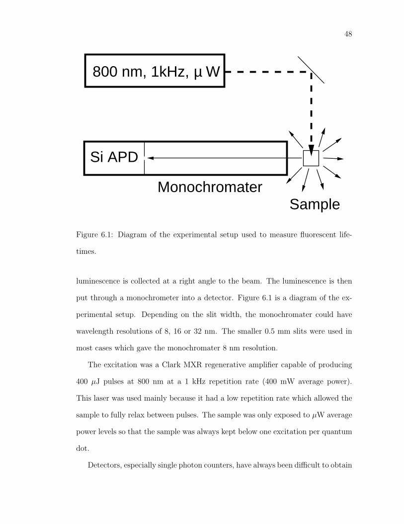
48

800 nm, 1kHz, Wµ

Si APD

MonochromaterSample

Figure 6.1: Diagram of the experimental setup used to measure fluorescent life-

times.

luminescence is collected at a right angle to the beam. The luminescence is then

put through a monochrometer into a detector. Figure 6.1 is a diagram of the ex-

perimental setup. Depending on the slit width, the monochromater could have

wavelength resolutions of 8, 16 or 32 nm. The smaller 0.5 mm slits were used in

most cases which gave the monochromater 8 nm resolution.

The excitation was a Clark MXR regenerative amplifier capable of producing

400 µJ pulses at 800 nm at a 1 kHz repetition rate (400 mW average power).

This laser was used mainly because it had a low repetition rate which allowed the

sample to fully relax between pulses. The sample was only exposed to µW average

power levels so that the sample was always kept below one excitation per quantum

dot.

Detectors, especially single photon counters, have always been difficult to obtain

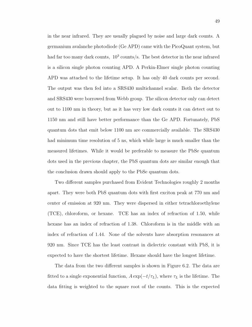
49

in the near infrared. They are usually plagued by noise and large dark counts. A

germanium avalanche photodiode (Ge APD) came with the PicoQuant system, but

had far too many dark counts, 103 counts/s. The best detector in the near infrared

is a silicon single photon counting APD. A Perkin-Elmer single photon counting

APD was attached to the lifetime setup. It has only 40 dark counts per second.

The output was then fed into a SRS430 multichannel scalar. Both the detector

and SRS430 were borrowed from Webb group. The silicon detector only can detect

out to 1100 nm in theory, but as it has very low dark counts it can detect out to

1150 nm and still have better performance than the Ge APD. Fortunately, PbS

quantum dots that emit below 1100 nm are commercially available. The SRS430

had minimum time resolution of 5 ns, which while large is much smaller than the

measured lifetimes. While it would be preferable to measure the PbSe quantum

dots used in the previous chapter, the PbS quantum dots are similar enough that

the conclusion drawn should apply to the PbSe quantum dots.

Two different samples purchased from Evident Technologies roughly 2 months

apart. They were both PbS quantum dots with first exciton peak at 770 nm and

center of emission at 920 nm. They were dispersed in either tetrachloroethylene

(TCE), chloroform, or hexane. TCE has an index of refraction of 1.50, while

hexane has an index of refraction of 1.38. Chloroform is in the middle with an

index of refraction of 1.44. None of the solvents have absorption resonances at

920 nm. Since TCE has the least contrast in dielectric constant with PbS, it is

expected to have the shortest lifetime. Hexane should have the longest lifetime.

The data from the two different samples is shown in Figure 6.2. The data are

fitted to a single exponential function, A exp(−t/τL), where τL is the lifetime. The

data fitting is weighted to the square root of the counts. This is the expected

50

0 5 10 15 20Time (µs)

10

100

1000

Cou

nts

TCE 2.4 µsHexane 2.8 µs

PbS QDs 770 nm Absorption Peak

0 5 10 15 20Time (µs)

10

100

1000

Cou

nts

TCE 2.1 µsChloroform 2.3 µsHexane 2.5 µs

PbS QDs 770 nm Absorption Peak

Figure 6.2: Data showing the variation of lifetime versus solvent.

51

error for a Poisson process. The data near the top of the curve is considered more

accurate than the data near the bottom and the fitting uses this. Also data with

less than around 10 to 100 counts were neglected in the fitting. The data with low

photon counts is suspect because of the influence of dark counts from the detector.

The lifetimes are offset, but clearly show that the lifetime of the quantum dots

in TCE is indeed shorter than that from chloroform or hexane. However, using the

simple classical model of dielectric screening, the quantum dots in hexane should

have 30% longer lifetime than that of the TCE. The actual result is just below 20%.

This could because the index of refraction given is not at the correct wavelength.

Also the classical model may not apply exactly to quantum dot systems. The work

with the CdSe/ZnS quantum dots implied a nonclassical dielectric screening[69].

The models put forward in that paper though neglect the dielectric constant of

the CdSe, and also would give a much smaller variation with respect to index of

refraction than is observed in this experiment with the PbS quantum dots[69].

While both samples show the approximately correct dielectric screening, they do

not have consistent lifetimes. This indicates that quantum dots are not being

synthesized consistently as of yet. Nonetheless, for these dots the lifetime can

be said to be approximately 2 µs long. This is relatively consistent with earlier

measurements on colloidal PbS quantum dots which measured 1 µs lifetimes[70].

6.3 Fluorescence Resonant Energy Transfer

When the PbS quantum dots that were studied are dried into a close packed film,

the luminescence red shifts from 920 nm by roughly 40 nm to 960 nm, as in Figure

6.3. It is believed that fluorescence (or Forster) resonant energy transfer (FRET)

is responsible for the shift. FRET uses the long range dipole-dipole interaction

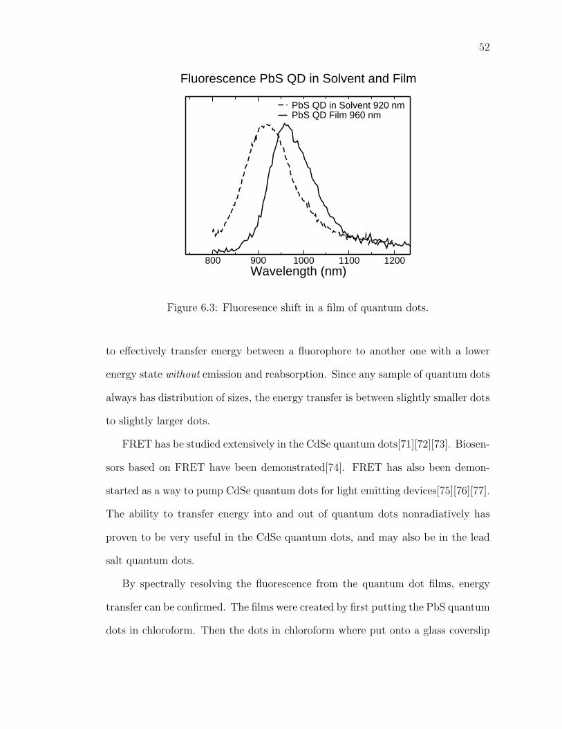
52

800 900 1000 1100 1200Wavelength (nm)

PbS QD in Solvent 920 nmPbS QD Film 960 nm

Fluorescence PbS QD in Solvent and Film

Figure 6.3: Fluoresence shift in a film of quantum dots.

to effectively transfer energy between a fluorophore to another one with a lower

energy state without emission and reabsorption. Since any sample of quantum dots

always has distribution of sizes, the energy transfer is between slightly smaller dots

to slightly larger dots.

FRET has be studied extensively in the CdSe quantum dots[71][72][73]. Biosen-

sors based on FRET have been demonstrated[74]. FRET has also been demon-

started as a way to pump CdSe quantum dots for light emitting devices[75][76][77].

The ability to transfer energy into and out of quantum dots nonradiatively has

proven to be very useful in the CdSe quantum dots, and may also be in the lead

salt quantum dots.

By spectrally resolving the fluorescence from the quantum dot films, energy

transfer can be confirmed. The films were created by first putting the PbS quantum

dots in chloroform. Then the dots in chloroform where put onto a glass coverslip

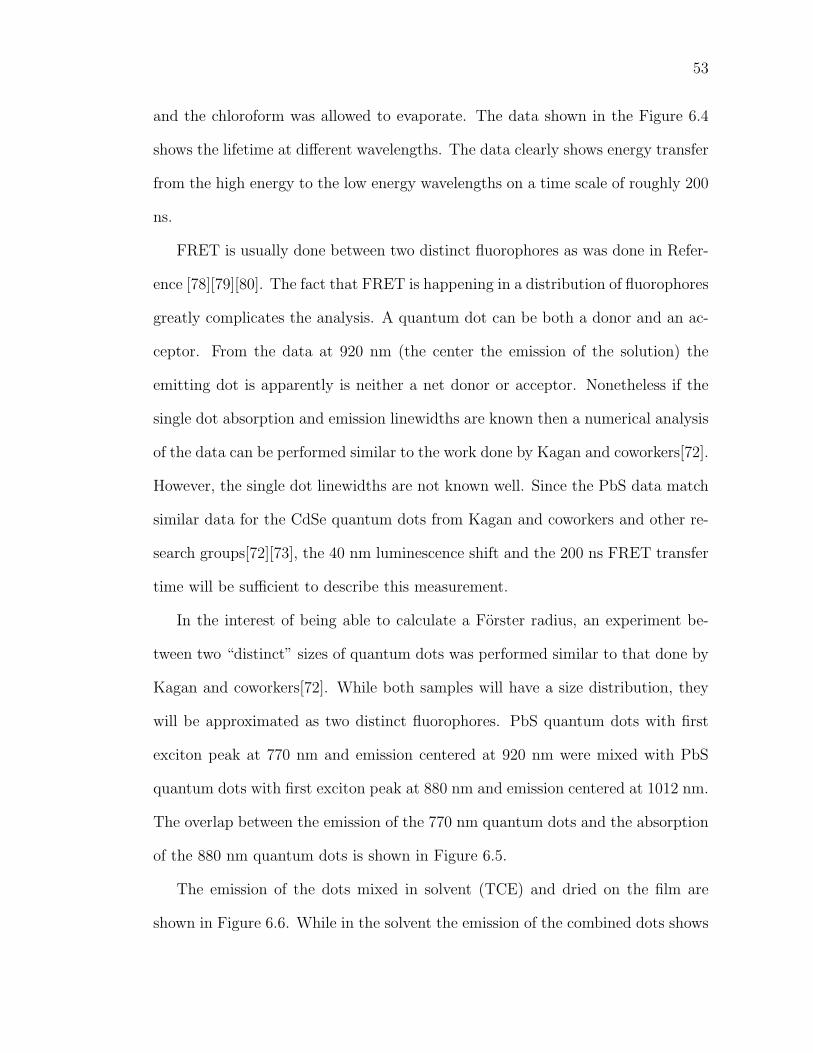
53

and the chloroform was allowed to evaporate. The data shown in the Figure 6.4

shows the lifetime at different wavelengths. The data clearly shows energy transfer

from the high energy to the low energy wavelengths on a time scale of roughly 200

ns.

FRET is usually done between two distinct fluorophores as was done in Refer-

ence [78][79][80]. The fact that FRET is happening in a distribution of fluorophores

greatly complicates the analysis. A quantum dot can be both a donor and an ac-

ceptor. From the data at 920 nm (the center the emission of the solution) the

emitting dot is apparently is neither a net donor or acceptor. Nonetheless if the

single dot absorption and emission linewidths are known then a numerical analysis

of the data can be performed similar to the work done by Kagan and coworkers[72].

However, the single dot linewidths are not known well. Since the PbS data match

similar data for the CdSe quantum dots from Kagan and coworkers and other re-

search groups[72][73], the 40 nm luminescence shift and the 200 ns FRET transfer

time will be sufficient to describe this measurement.

In the interest of being able to calculate a Forster radius, an experiment be-

tween two “distinct” sizes of quantum dots was performed similar to that done by

Kagan and coworkers[72]. While both samples will have a size distribution, they

will be approximated as two distinct fluorophores. PbS quantum dots with first

exciton peak at 770 nm and emission centered at 920 nm were mixed with PbS

quantum dots with first exciton peak at 880 nm and emission centered at 1012 nm.

The overlap between the emission of the 770 nm quantum dots and the absorption

of the 880 nm quantum dots is shown in Figure 6.5.

The emission of the dots mixed in solvent (TCE) and dried on the film are

shown in Figure 6.6. While in the solvent the emission of the combined dots shows

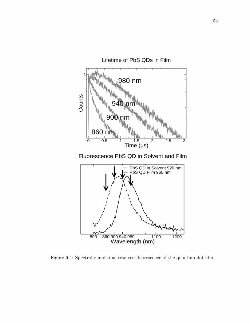
54

0 0.5 1 1.5 2 2.5 3Time (µs)

1

Cou

nts

Lifetime of PbS QDs in Film

980 nm

940 nm

900 nm

860 nm

800 860 900 940 980 1100 1200Wavelength (nm)

PbS QD in Solvent 920 nmPbS QD Film 960 nm

Fluorescence PbS QD in Solvent and Film

Figure 6.4: Spectrally and time resolved fluorescence of the quantum dot film.

55

700 800 900 1000 1100 1200λ (nm)

Absorbance of 880 nm dotsEmission on 770 nm dots

Overlap of Absorbance and Emission

Figure 6.5: Overlap of the emission from the 770 nm qauntum dots with the

absorbance of the 880 nm quantum dots.

a superposition of the individual emission spectra, the dots dried in film show

emission that looks similar to the emission of the 880 nm dots only. The shift in

luminescence is from 950 nm in solution by 100 nm to 1050 nm.

To calculate a Forster radius, R0, the formula as followed is used[81].

R60 =

9000κ2 ln 10

128π6n4NAV

Φd

∫ ∞

0Ed(ν)εa(ν)

dν

ν4(6.1)

κ2 is an orientation factor that is assigned 2/3. NAV is Avogadro’s number. Φd is

the quantum yield of the donor. Ed(ν) is the normalized donor emission spectra.

εa(ν) is the molar extinction coefficient of the acceptor. There some uncertainity

in some of these numbers. The concentration is not known but is estimated from

the size of the quantum dots and the known mass of lead salt per mL. This gives

an estimated εa at the first exciton peak of 8×104M−1cm−1. The quantum yield is

taken to be around 50 % but it is not known. Given data from Reference [68], 50%

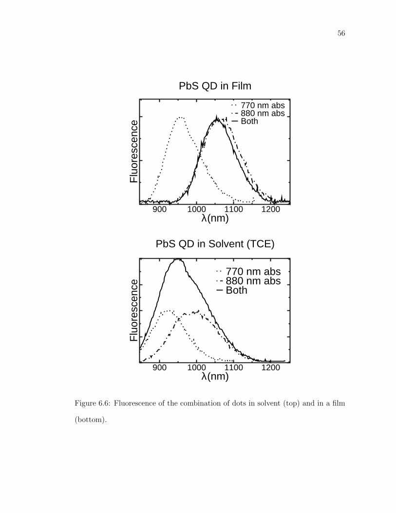
56

900 1000 1100 1200λ(nm)

Flu

ores

cenc

e

770 nm abs880 nm absBoth

PbS QD in Film

900 1000 1100 1200λ(nm)

Flu

ores

cenc

e

770 nm abs880 nm absBoth

PbS QD in Solvent (TCE)

Figure 6.6: Fluorescence of the combination of dots in solvent (top) and in a film

(bottom).

57

is not unreasonable. The quantum yield is not easily measured for a fluorophore

in the near infrared. The overlap integral is calculated with the absorption and

emission from Figure 6.5 with the assumption that there are only two fluorophores.

The actual integral should be over the single particle absorption and emission. This

calculation is only to get a rough idea of the Forster radius. With all the numbers

put into the equation a Forster radius of 80A is calculated. Note due to the

sixth power in the exponent, a 50% error in the calculation is only a 7A error

in the radius. The calculated Forster radius is within an order of magnitude of a

reasonable number.

Spectrally resolving the fluorescence again shows the energy tranfer. The data

is shown in Figure 6.7. The transfer time appears to be between 200 and 400 ns.

The theoretical transfer time is given by the equation:

τ = τd

(R

R0

)6

(6.2)

In the equation τd is the lifetime of the donor taken to be 2.5 µs. This gives a

separation distance between 50 and 60 A. Even though the estimate is quite rough,

it gives a distance that is quite plausible for a close packed quantum dot film.

Another way to look at the previous experiment is to think of the two dots

together not as two dots, but as one sample of dots with a large size distribution.

The much larger spectral shift fits well with the calculated work done by Kagan

and coworkers[72]. A larger size distribution leads to a larger spectral shift.

6.4 Conclusion

The PbS quantum dots have long lifetimes, around 2 µs. Dielectric screening

can explain this fact, and dielectric screening can also help explain the lack of a

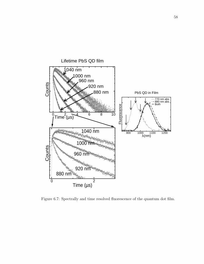
58

0 2 4 6 8 10Time (µs)

Cou

nts

Lifetime PbS QD film

1040 nm1000 nm

960 nm920 nm

880 nm

900 1000 1100 1200λ(nm)

Flu

ores

cenc

e

770 nm abs880 nm absBoth

PbS QD in Film

0 2Time (µs)

Co

un

ts

880 nm920 nm

960 nm

1040 nm

1000 nm

Figure 6.7: Spectrally and time resolved fluorescence of the quantum dot film.

59

nonlinear signal measured. The PbS quantum dots exhibit FRET very similar to

the CdSe quantum dots. The FRET times are longer because the lifetimes are

longer. If more were known about the intrinsic properties of the PbS, then a more

detailed analysis similar to Kagan and coworkers[72] could be performed. It would

also be beneficial if the lifetime of the dots in solvent were consistent between

samples produced at different times.

While it is important to verify that FRET takes place in PbS films and that

it is the cause of the luminescence shift, the there is no novelty in the observation

because it so closely mirrors the work done with the CdSe quantum dots. The

really interesting work is to use FRET to transfer energy into the quantum dots

from other sources similar to the work done by Klimov’s group [75][76] and by

Anni and coworkers[77]. Questions such how does dielectric screening affect the

transfer times, and what effect does the large difference in lifetimes between donor

and acceptor mean for applications, will have to be answered.

While the lead salt quantum dots do not look favorable as nonlinear materials,

the future of the lead salt quantum dots looks quite promising. Recent research

by other groups such as impact ionization in the lead salts that may lead to more

efficient solar cells will help keep the field strong for several more years[82].

APPENDIX A

METHODS FOR ENCAPSULATING QUANTUM DOTS IN LIPIDS

A.1 Introduction

The encapsulating procedure is based roughly on the work of Dubertret and

coworkers [14]. It involves three main steps. Washing is performed to get rid

of excess ligand. Then the actual encapsulation step is next. Then a filtering step

is performed last of all.

Unless otherwise noted, all lipids came from Avanti Polar Lipids of Alabaster,

Alabama. The quantum dots were donated by Professor Todd Krauss of Rochester

University. Care must be taken in using this synthesis with dots from other sources.

Coworkers in the Wise group lab, Byung-Ryool Hyun and Sareet Jacob[83], found

that to encapsulate quantum dots from Evident Technologies, ligand exchange had

to be performed.

A.2 Washing the Dots

Washing the dots is actually a method to remove the excess ligand, which is usually

trioctylphosphine oxide (TOPO), from solution. The dots are grown in a solution

that is rich in TOPO and they are usually stored and shipped in solution with

excess TOPO. The excess TOPO in the solution helps keep the dots stable over

several months. Therefore one should wash the dots only before they plan to

encapsulate them. Washed dots last at least a few weeks.

If the excess TOPO is not removed from the solution, the dots will not be

encapsulated. TOPO is very hydrophobic, and if there is excess, the lipids will

form micelles around the free TOPO and not the quantum dots. The result is

60

61

a foamy solution of TOPO-lipid micelles and quantum dot aggregates. However,

washing the dots also can damage them. If the dots are washed too often, too

much TOPO will be removed from the dots. Then the dots will precipitate out

of the nonpolar organic solvents. The dots without the TOPO aren’t hydrophobic

enough, and won’t form a micelle. The water will then destroy them. Depending

on the source of quantum dots, one may have to wash the dots slightly differently

as different sources may have differing amounts of ligand with the quantum dots.

The basic concept of washing is that the dots are put into a slightly polar

solvent, methanol. Then the dots are centrifuged. The dots end up on the bottom

of the centrifuge tube and excess TOPO is left in solution which is then removed.

The precipitated quantum dots are then reintroduced to a nonpolar organic solvent.

If they haven’t been washed too many times, they will go back into solution. A

little experimentation may be required to get the washing correct when dealing

with a new source of quantum dots.

The quantum dots came from Professor Krauss in hexane at 15 µM. The dot to

slightly polar solvent ratio used in washing was 1 to 3. Since a microcentrifuge that

held 1.5 mL eppendorf tubes was used to precipitate the quantum dots, 700 µL of

dots were washed at a time. 350 µL of dots was mixed with 997.5 µL methanol

and 52.5 µL of butanol and put into a tube. On the advise of Professor Krauss

a small amount of butanol was used. Methanol by itself seemed to work fine as

well though. The 1.4 mL of solution was put into two 1.5 mL eppendorf tubes.

The two tubes were put into the centrifuge opposite each other for balance. The

centrifuge was then run at 10,000 rpm for 5 minutes. After that, the dots were

at the bottom of the eppendorf tube. The solution was poured off, and 350 µL of

hexane was put into the tube. After a slight shake the quantum dots went back

62

into solution. This step was performed three times and then the dots were stored

in a glass vial until they were used.

A.3 Encapsulating the Dots

Encapsulating the dots is quite straightforward. Washed dots were mixed with

the lipids which were in chloroform in a glass vial or test tube. The lipid to dot

ratio was around 2000 to 1. Then excess chloroform was added to the mixture.

The reason for the extra chloroform is that the dot lipid mixture when evaporated

must form a thin film on the glass. If the film is thick, the dots will be aggregated

when the water is added and usually stay that way. Typical numbers were 25 µL

of dots with 400 µL of excess chloroform plus whatever chloroform came with the

lipids. The actual amount of extra chloroform added depends on the glass tube

used. The extra 400 µL is for a 4 mL glass vial. If a different glass tube or vial is

used, the extra chloroform needed may have to be adjusted.

The mixture is evaporated under nitrogen in a fume hood. Then clean water

at room temperature is added and the mixture is covered. The mixture is allowed

to sit at room temperature overnight. Temperature is expected to play a part in

the self-assembly of the lipid-dot micelles, but experimentally temperature didn’t

seem to matter much. It is worth more investigation though. The next day the

mixture was quickly, less than 30 seconds, ultrasonicated. Too much sonication

will also kill the dots. Then the dots are ready to be filtered.

A table of lipid combinations that worked is listed in Table A.1. The first

column is the amount of single chain lipid used. LMPC has a single 14 unit fully

saturated hydrocarbon chain with the phosphatidylcholine head group. The sec-

ond column is the double chain lipid used. DMPC has a double chain 14 units long

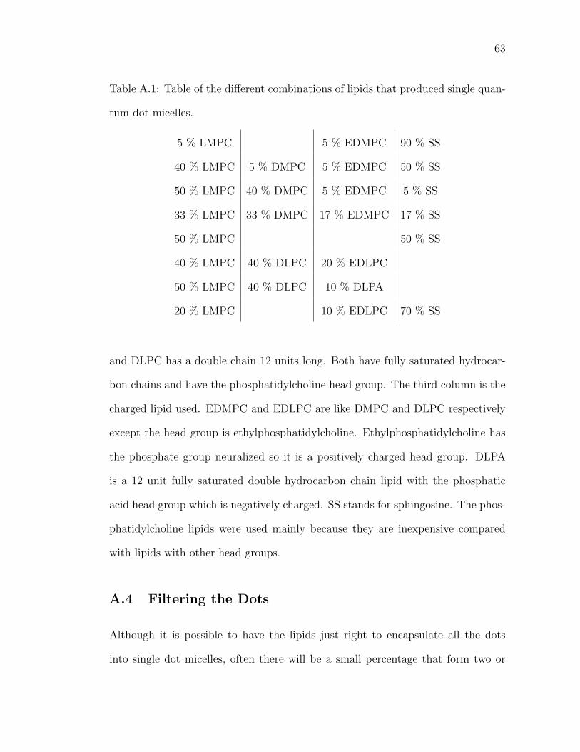
63

Table A.1: Table of the different combinations of lipids that produced single quan-

tum dot micelles.

5 % LMPC 5 % EDMPC 90 % SS

40 % LMPC 5 % DMPC 5 % EDMPC 50 % SS

50 % LMPC 40 % DMPC 5 % EDMPC 5 % SS

33 % LMPC 33 % DMPC 17 % EDMPC 17 % SS

50 % LMPC 50 % SS

40 % LMPC 40 % DLPC 20 % EDLPC

50 % LMPC 40 % DLPC 10 % DLPA

20 % LMPC 10 % EDLPC 70 % SS

and DLPC has a double chain 12 units long. Both have fully saturated hydrocar-

bon chains and have the phosphatidylcholine head group. The third column is the

charged lipid used. EDMPC and EDLPC are like DMPC and DLPC respectively

except the head group is ethylphosphatidylcholine. Ethylphosphatidylcholine has

the phosphate group neuralized so it is a positively charged head group. DLPA

is a 12 unit fully saturated double hydrocarbon chain lipid with the phosphatic

acid head group which is negatively charged. SS stands for sphingosine. The phos-

phatidylcholine lipids were used mainly because they are inexpensive compared

with lipids with other head groups.

A.4 Filtering the Dots

Although it is possible to have the lipids just right to encapsulate all the dots

into single dot micelles, often there will be a small percentage that form two or

64

more dots per micelle. In order to get rid of the non-single dot micelles, filtering is

performed. Syringe filters from Millipore were used. The membrane filters that fit

into the syringe are disposable and the syringe is reusable. Two filters were used

from Millipore, one with 220 nm pore and the other with a 25 nm pore. Unless

the method of encapsulating is known to produce mostly single QD micelles, the

220 nm pore filter is used first. This gets rid of any large aggregates that may

clog the smaller filter. Also these are 60% cheaper than the 25 nm pore filters. If

the quantum dots don’t go through this filter or are very difficult to go through

this filter, then the lipid mixture won’t work. The smaller filter is then used. If a

substantial number of quantum dots go through the filter (and this is checked by

a fluorometer or a UV lamp), then the encapsulation procedure worked.

Fluorescence correlation spectroscopy was performed both before and after the

filtering on many samples. Only a few samples could have simple diffusion fits

without filtering. Most encapsulation procedures that worked often would have

one or two quantum dot aggregrates go through the diffusion volume in the five

minutes it took to take data. Only one aggregate is enough to alter the FCS curve.

With filtering, the encapsulated quantum dots produce clean FCS curves.

BIBLIOGRAPHY

[1] C. B. Murray, D. J. Norris, and M. G. Bawendi, J. Am. Chem. Soc. 115, 8706(1993).

[2] C. B. Murray, S. H. Sun, W. Gaschler, et al., IBM J. Res.Dev. 45, 47 (2001).

[3] S. Kim and M. G. Bawendi, J. Am. Chem. Soc. 125, 14652 (2003).

[4] H. Mattoussi, J. M. Mauro, E. R. Goldman, G. P. Anderson, V. C. Sundar,F. V. Mikulec, and M. G. Bawendi, J. Am. Chem. Soc. 122, 12142 (2000).

[5] A. L. Efros and A. L. Efros, Sov. Phys. Semicond. 16, 772 (1982).

[6] L. E. Brus, J. Chem. Phys. 80, 4403 (1984).

[7] S. Schmitt-Rink, D. A. B. Miller, and D. S. Chemla, Phys. Rev. B 35, 8113(1987).

[8] M. Brumer, A. Kigel, L. Amirav, A. Sashchiuk, O. Solomesch, N. Tessler, andE. Lifshitz, Adv. Funct. Mater. 15, 1111 (2005).

[9] S. M. Sze, Physics of Semiconductor Devices (Wiley, New York, 1981).

[10] M. A. Hines and P. Guyot-Sionnest, J. Phys. Chem. 100, 468 (1996).

[11] X. Peng, J. Wickham, and A. P. Alivisatos, J. Am. Chem. Soc. 120, 5343(1998).

[12] M. Bruchez Jr., M. Moronne, P. Gin, S. Weiss, and A. P. Alivisatos, Science281, 2013 (1998).

[13] W. C. W. Chan and S. Nie, Science 281, 2016 (1998).

[14] B. Dubertret, P. Skourides, D. J. Norris, V. Noireaux, A. H. Brrivanlou, andA. Libchaber, Science 298, 1759 (2002).

[15] W. C. W. Chan, D. J. Maxwell, X. Gao, R. E. Bailey, M. Han, and S. Nie,Curr. Opin. Biotechnol. 13, 40 (2002).

[16] V. L. Colvin and A. P. Alivisatos, J. Chem. Phys. 97, 730 (1992).

[17] V. L. Colvin, K. L. Cunningham, and A. P. Alivisatos, J. Chem. Phys. 101,7122 (1994).

[18] V. L. Colvin, Ph.D. thesis, University of California at Berkeley, 1994.

[19] S. A. Empedocles and M. G. Bawendi, Science 278, 2114 (1997).

65

66

[20] X. Wu, H. Liu, J. Liu, K. N. Haley, J. A. Treadway, J. P. Larson, N. Ge,F. Peale, and M. P. Bruchez, Nature Biotechnol. 21, 41 (2003).

[21] M. Nirmal, B. O. Dabbousi, M. G. Bawendi, J. J. Macklin, J. K. Trautman,T. D. Harris, and L. E. Brus, Nature 383, 802 (1996).

[22] D. R. Larson, W. R. Zipfel, R. M. Williams, S. W. Clark, M. P. Bruchez,F. W. Wise, and W. W. Webb, Science 300, 1434 (2003).

[23] D. R. Larson, Ph.D. thesis, Cornell University, 2004.

[24] W. W. Webb, Appl. Opt. 40, 3969 (2001).

[25] H. Mattoussi, A. W. Cumming, C. B. Murray, M. G. Bawendi, and R. Ober,Phys. Rev. B 58, 7850 (1998).

[26] M. Pelton, D. G. Grier, and P. Guyot-Sionnest, Appl. Phys. Lett. 85, 819(2004).

[27] M. Kuno, D. P. Fromm, H. F. Hamann, A. Gallagher, and D. J. Nesbitt, J.Chem. Phys. 112, 3117 (2000).

[28] T. J. Rink, C. Montecucco, T. R. Hesketh, and R. Y. Tsien, Biochim. Biophys.Acta 595, 15 (1980).

[29] E. F. Fluhler, V. G. Burnham, and L. M. Loew, Biochemistry 24, 5749 (1985).

[30] H. T. Tien, Bilayer Lipid Membranes (BLM): Theory and Practice (Dekker,New York, 1974).

[31] L. Moreaux, T. Pons, V. Dambrin, M. Blanchard-Desce, and J. Mertz, Opt.Lett. 28, 625 (2003).

[32] L. Mathivet, S. Cribier, and P. E. Devaux, Biophys. J. 70, 1112 (1996).

[33] K.-i. Akashi, H. Miyata, H. Itoh, and K. Kinosita Jr., Biophys. J. 71, 3242(1996).

[34] T. J. Rink, C. Montecucco, T. R. Hesketh, and R. Y. Tsien, Biochim. Biophys.Acta 595, 15 (1980).

[35] C. Bronner and Y. Landry, Biochim. Biophys. Acta 1070, 3321 (1991).

[36] A. H. Merill, Jr., E-M. Schmelz, D. L. Dillehay, S. Spiegel, J. A. Shayman,J. J. Schroeder, R. T. Riley, K. A. Voss, and E. Wang, Toxicology and AppliedPharmacology 142, 208 (1997).

[37] J. N. Israelachvili, Intermolecular and Surface Forces (Academic Press, Or-lando, 1985), pp. 229-275.

67

[38] K. Holmberg, B. Jonsson, B. Kronberg, and B. Lindman, Surfactants andPolymers in Aqueous Solution (John Wiley & Sons, Ltd, West Sussex, England,2003).

[39] C. Tanford, The Hydrophobic Effect: Formation of Micelles and BiologicalMembranes (Wiley, New York 1980).

[40] D. Marsh, CRC Handbook of Lipid Bilayers (CRC Press, Boca Raton, FL,1990), p. 276-279.

[41] K. Sou, T. Endo, S. Takeoka, and E. Tsuchida, Bioconjugate Chem. 11, 372(2000).

[42] H. Heerklotz and R. M. Epand, Biophys. J. 80, 271 (2001).

[43] J. Eastoe and J. S. Dalton, Langmuir 14, 5719 (1998).

[44] D. S. Johnston, S. Sanghera, M. Pons, and D. Chapman, Biochim. Biophys.Acta 602, 57 (1980).

[45] Y. Kang and T. A. Taton, J. Am. Chem. Soc. 125, 5650 (2003).

[46] R. C. MacDonald, G. W. Ashley, M. M. Shida, V. A. Rakhmanova, Y. S. Tara-hovsky, D. P. Pantazatos, M. T. Kennedy, E. V. Pozharski, K. A. Baker,R. D. Jones, H. S. Rosenzweig, K. L. Choi, R. Qui, and T. J. McIntosh, Biophys.J. 77, 2612 (1999).

[47] D. A. Dombeck, M. B.-Desce, and W. W. Webb, J. Neurosci. 24, 999 (2004).

[48] M. Han, X. Gao, J. Z. Su, and S. Nie, Nature Biotechnol. 19, 631 (2001).

[49] Landolt-Bornstein: Numerical Data and Functional Relationships in Scienceand Technology, New Series edited by O. Madelung, M. Schultz, and H. Weiss(Springer-Verlag, 1982).

[50] F. W. Wise, Acc. Chem. Res. 33, 773 (2000).

[51] I. Kang and F. W. Wise, J. Opt. Soc. Am. B 14, 1632 (1997).

[52] G. Allan and C. Delerue, Phys. Rev. B 70, 245321 (2004).

[53] L. E. Brus, Appl. Phys. A 53, 465 (1991).

[54] V. Klimov in Handbook on Nanostructured Materials and Nanotechnology,H. Nalwa, ed., (Academic Press, San Diego, CA, 1999) Volume 4, p 451.

[55] M. Yamane and Y. Asahara, Glasses for Photonics (Cambridge UniversityPress, Cambridge, United Kingdom, 2000).

68

[56] P. T. Guerreiro, S. Ten, N. F. Borrelli, J. Butty, G. E. Jabbour, andN. Peyghambarian, Appl. Phys. Lett. 71, 1595 (1997).

[57] K. Wundke, S. Potting, J. Auxier, A. Schulzgen, N. Peyghambarian, andN. F. Borelli, Appl. Phys. Lett. 76, 10 (2000).

[58] J. F. Philipps, T. Topfer, H. Ebendorff-Heidepriem, D. Ehrt, R. Sauerbrey,and N. F. Borrelli, Appl. Phys. B 72 175 (2001).

[59] A. M. Malyarevich, V. G. Savitski, P. V. Prokoshin, N. N. Posnov, K. V. Yu-mashev, E. Raaben, and A. A. Zhilin, J. Opt. Soc. Am. B 19 28 (2002).

[60] G. P. Agrawal, Nonlinear Fiber Optics (Academic Press, San Diego, California1995) p 583.

[61] M. Sheik-Bahae, A. A. Said, T.-H. Wei, D. J. Hagan, and E. W. Van Stryland,IEEE J. Quantum Electron. 26, 760 (1990).

[62] I. Kang, T. Krauss, and F. Wise, Opt. Lett. 22, 1077 (1997).

[63] C. H. Kwak, Y. L .Lee, and S. G. Kim, J. Opt. Soc. Am. B 16, 600 (1999).

[64] M. Falconieri, J. Opt. A: Pure Appl. Opt. 1, 662 (1999).

[65] S. Alves, A. Bourdon, and A. M. Figueiredo Neto, J. Opt. Soc. Am. B 20,713 (2003).

[66] J. Wang, M. Sheik-Bahae, A. A. Said, D. J. Hagan, and E. W. Van Stryland,J. Opt. Soc. Am. B 11, 1009 (1994).

[67] J. M. Harbold, F. O. Ilday, F. W. Wise, J. S. Sanghera, V. Q. Nguyen,L. B. Shaw, and I. D. Aggarwal, Opt. Lett. 27, 119 (2002).

[68] B. L. Wehrenberg, C. Wang, and P. Guyot-Sionnest, J. Phys. Chem. B 106,10634 (2002).

[69] S. F. Wuister, C. de Mello Donega, and A. Meijerink, J. Chem. Phys. 121,4310 (2004).

[70] J. H. Warner, E. Thomsen, A. R. Watt, N. R. Heckenberg, and H. Rubinsztein-Dunlop, Nanotechnology 16, 175 (2005).

[71] C. R. Kagan, C. B. Murray, M. Nirmal and M. G. Bawendi, Phys. Rev. Lett.76, 1517 (1996).

[72] C. R. Kagan, C. B. Murray, and M. G. Bawendi, Phys. Rev. B 54, 8633(1996).

[73] S. A. Crooker, J. A. Hollingsworth, S. Tretiak, and V. I. Klimov, Phys. Rev.Lett. 89, 186802 (2002).

69

[74] I. L. Medintz, A. R. Clapp, H. Mattoussi, E. R. Goldman, B. Fisher, andJ. M. Mauro, Nature Materials 2, 630 (2003).

[75] M. Achermann, M. A. Petruska, S. Kos, D. L. Smith, D. D. Koleske, andV. I. Klimov, Nature 429, 642 (2004).

[76] S. Kos, M. Achermann, V. I. Klimov, and D. L. Smith, Phys. Rev. B 71,205309 (2005).

[77] M. Anni, L. Manna, R. Cingolani, D. Valerini, A. Creti, and M. Lomascolo,Appl. Phys. Lett 85, 4169 (2004).

[78] R. C. Powell and R. G. Kepler, Phys. Rev. Lett. 22, 636 (1969).

[79] P. Wu and L. Brand, Anal. Biochem. 218, 1 (1994).

[80] R. M. Clegg, Curr. Opin. Biotechnol. 6, 103 (1995).

[81] T. Forster, Discuss. Faraday Soc. 27, 7 (1959).

[82] R. D. Schaller and V. I. Klimov, Phys. Rev. Lett. 92, 186601 (2004).

[83] B.-R. Hyun and S. Jacob (private communication).