Colloid Stability

8/3/2019 Colloid Stability

http://slidepdf.com/reader/full/colloid-stability 1/14

Chapter 3

Colloid Stability

John Eastman

3.1 Introduction

One of the important aspects of the study of colloidal dispersions is understanding their

stability so that we can manipulate the state of dispersions for particular applications.

Charge stabilisation is one means by which this can be achieved and we can manipulate

the stability through changes in the chemical environment such as salt concentration, ion

type and pH.

We must understand how this works both in quiescent systems and when external fields,

such as gravitational or shear fields, are present.

So what do we mean by stability? This very much depends on the circumstances which

are being considered. We can define stability in colloidal systems either in terms of their

tendency to aggregate or in terms of their tendency to sediment under the action of gravity.

In this chapter we will focus on the stability to aggregation and look at the factors which

control this stability. We will study this by considering the interaction between two rep-

resentative particles in the system. By considering what happens when two particles come

together (during a Brownian collision) we can predict the stability of the whole system by

looking at the form of the colloidal pair potential.

3.2 The Colloidal Pair Potential

The pair potential is the total potential energy of interaction between two colloidal particles

as the separation or distance between them is varied. Formally it is a free energy, and we

calculate it by simply summing the various components that we can identify.

The calculation is normally done for two particles in isolation, i.e. at infinite dilution. In

a concentrated system (a condensed phase), multi-body interactions should be accounted

for, and then we would refer to the potential of mean force. However we get an adequate

estimation of the total potential in a concentrated system simply by the summation of the

interaction from the nearest neighbours.

It is this interaction energy that governs the stability of colloidal dispersions and which

we effectively manipulate whenever we make a change to a formulation.



Colloid Stability 37

The components of the pair potential that we are most interested in for charged colloids

are those due to the attractive van der Waals forces and the repulsive force between similarly

charged particles.

3.2.1 Attractive forces

Molecules with a permanent dipole will attract similar molecules as the dipoles align. They

will also induce a dipole in an adjacent neutral atom or molecule and cause an attraction.

This is relatively easy to understand; however, the motion of the electrons in any atom cause

rapidly fluctuating dipoles. This leads to the London dispersion interaction as the oscillating

dipoles become coupled. Even neutral atoms have a fluctuating dipole due to the motion

of the electrons around the nucleus. It is energetically more favourable for adjacent atoms

to be oscillating in unison. This is the interaction which we recognise from the non-ideal

behaviour of the inert gases.This interaction is non-directional, so that when large assemblies of atoms are considered,

different dipolar orientations do not cancel each other. Colloidal particles are of course

large assemblies of atoms and hence the van der Waals forces from the London dispersion

interaction act between particles to cause attraction (see Figure 3.1).

The early calculations were due to Hamaker and de Boer [1]. The route is to sum the

interaction of one atom in a particle with each atom in the adjacent particle. That interaction

is then summed over all the atoms in the first particle.

The result is a long range interaction – much longer range than the interaction between

two isolated atoms. The range of the interaction is comparable with the radii of colloidal

particles.

The attractive potential energy is directly proportional to a particle radius (a ), a material

constant – the Hamaker [1] constant ( A) – and is inversely proportional to distance of

separation (h):

V A = −A

12

1

x (x + 2)+

1

(x + 1)2+ 2 ln

x (x + 2)

(x + 1)2

, where x =

h

2a (3.1)

When the particle separation is small (h 2a ) this reduces to a simple form of

V A = −Aa

12h(3.2)

a h

Figure 3.1 London forces between atoms in two adjacent colloidal particles.



38 Colloid Science: Principles, Methods and Applications

Table 3.1 Hamaker constants for various materials

Particles Hamaker constant (J/10−20) Media Hamaker constant ( J/10−20)

Poly(tetrafluorethylene) 3.8 Water 3.7Poly(methyl methacrylate) 7.1 Pentane 3.8

Poly(styrene) 7.8 Ethanol 4.2

Silica (fused) 6.5 Decane 4.8

Titanium dioxide 19.5 Hexadecane 5.1

Metals (Au, Ag, Pt, etc.) ∼40 Cyclohexane 5.2

The Hamaker constant is a function of both the electronic polarisability and the density of

the material. When particles are immersed in a medium the attraction between particles

is weakened as there is an attraction with the medium also. The combined or compositeHamaker constant ( A) can be estimated as the geometric mean of that of the particle

( Aparticle) and that of the medium ( Amedium) with respect to their values in vacuum, and it

is this that should be used in the calculation of the attractive potential:

A = (

Aparticle −

Amedium)2 (3.3)

Hamaker constants have values in the range of 10−20 J, and a selection of values are given in

Table 3.1.

3.2.2 Electrostatic repulsion

Electrical repulsion is an important stabilising mechanism for particles dispersed in aqueous

solutions or moderate polarity liquids like ethylene glycol.

The diffuse part of the electrical double layer extends in solution over distances charac-

terisedbytheDebyelength(1/κ). In practice we usethe experimentallyaccessibleζ -potential

(see Section 3.3.3) as a measure of the electrical potential at the Stern layer. The rate of de-

cay of this potential is governed by the reciprocal of the Debye length and is commonly

referred to as the double layer thickness (see Table 3.2). This defines the extent to which the

ionic atmosphere, which is different from the bulk ionic medium, extends from the particle

surface.

Table 3.2 The extent of the double layer thickness as a function

of electrolyte concentration

NaCl Concentration (mM) Double layer thickness (nm)

30 2

10 3

1 10

0.1 30




Figure 3.2 The overlap of electrical double layers in adjacent particles.

Whentwoparticlesapproacheachothertheionicatmospheresoverlap(seeFigure3.2)and

the local ion concentration midway between the particles can be estimated by summing the

contributions from each particle. The difference in this local mid-point ion concentration

and that in the bulk results in an osmotic pressure acting to force the particles apart.

Integration of this force with respect to distance gives us the energy.

When two charged particles come together there are two extreme cases which we can

envisage. If the ion adsorption equilibrium is maintained then either the surface charge

remains constant and the surface potential compensates (constant charge) or the surface

potential remains constant and the surface charge density changes to compensate (constant

potential). Hogg et al . [2] derived expressions which enable us to calculate the interaction

between non-identical spheres under both constant charge and constant potential condi-

tions.

V ψ

R =εa 1a 2

ψ2

01+ψ2

02

4(a 1 + a 2)

2ψ01

ψ02

ψ201+ψ2

02

ln

1+ exp(−κh)

1− exp(−κh)

+ ln(1− exp(−2κh))

(3.4)

V σ

R

=εa 1a 2ψ

201+ψ2

024(a 1 + a 2)

2ψ01ψ02

ψ201 +ψ202

ln1+ exp(−κh)

1− exp(−κh)− ln(1− exp(−2κh)) (3.5)

These reduce to the basic expressions

V ψ

R =εa ψ2

0

2ln(1 + exp(−κh)) (3.6)

V σ R = −εa ψ2

0

2ln(1 − exp(−κh)) (3.7)

for the interaction between identical particles with a radius a . The expressions are valid in

the regime where κa , the product of the Debye constant and the particle radius, is greater

than 10.




For conditions where κa is less than 3 the general expression is

V R = 2πεa ψ2δ exp(−κh) (3.8)

3.2.3 Effect of particle concentration

Whenever we add charged colloidal particles to a liquid we do two things:

r add counter-ions with each particle r reduce the solution volume available to the ions.

Both of these factors become important as the particle concentration increases and when

the background electrolyte concentration is low. We can expand the expression for κ from

Equation (2.18), Chapter 2, to take account of these extra effects. The expanded expression is

κ2 =e 2z 2

εk B T

2n0 +3|σ δ|φ

ae 1− φ

(3.9)

where z is the counter-ion valency, n0 the concentration of counter-ions in solution (added

electrolyte), a is the particle radius and e is the formal charge on an electron.

We recognise the first part of the expression from Equation (2.18) but now we have the

expression 3|σ δ |φae

which takes into account the counter-ions which are carried by the particle

through the surface charge density σ δ . We can see that this expression becomes important

when the particles are small and the volume fraction φ and surface charge density are high.The denominator of (1 – φ) takes into account the volume taken up by the particles in the

dispersion.

This effect is only important when the background electrolyte levels are low and where we

have high concentrations of small highly charged particles. We can see the effect in Figure 3.3

which shows the effect for different background electrolytes as a function of particle volume

fraction for 85 nm radius particles with a surface charge density of 0.15 µC cm−2.

3.2.4 Total potential

The linear addition of the electrostatic and dispersion potentials is the basis of the DLVO

[3, 4] theory for colloid stability. When we add the attractive potential to the repulsive

electrostatic potential we have the typical curve for charge stabilised colloidal particles:

V T = V A + V R (3.10)

This curve has a number of interesting and important features. The shape of the curve is the

consequence of the addition of the exponential decay of the repulsive term and the more

steeply decaying one-over-distance relationship of the attractive term.

This linear superposition leads to a maximum in the curve as seen in Figure 3.4 and is

known as the primary maximum. It is this maximum in the pair potential which provides




ϕ

0.0 0.1 0.2 0.3 0.4 0.5

2.0 × 10−9

1 / κ ( m

− 1 )

4.0 × 10

−9

6.0 × 10−9

8.0 × 10−9

1.0 × 10−8

1.2 × 10−8

1.4 × 10−8

5 × 10−4 M

10−3 M

[NaCl] = 10−2 M

Figure 3.3 The effect of the counter-ions associated with the particle surface on the Debye length 1/ κ .

0.0 0.5 1.0 1.5 2.0 2.5 3.0 3.5 4.0

−60

−40

−20

0

20

40

60

80

100

120

140

V T

( k B

T )

κh (nm)

Figure 3.4 Examples of a total interaction potential curve for two charge stabilised systems.




the mechanism for stability of charged colloidal particles. It creates an effective activation

energy for aggregation. As two particles come together they must collide with sufficient

energy to overcome the barrier provided by the primary maximum.

It is important to realise that this barrier to aggregation only provides kinetic stability to

a dispersion. The thermodynamic drive is towards an aggregated, phase separated state. Wecan say that the larger the barrier the longer the system will remain stable.

Note that the potential is plotted in units of k B T . These thermal energy units help us

relate the height of the maximum with the energy of a Brownian collision, which will be of

the order of 1.5k B T .

Therefore, in order to pose a suitable barrier to aggregation this primary maximum

must be at least 1.5k B T . In practice we need to manipulate the system so that the primary

maximum is at least 20k B T in order to achieve a level of stability which can be relied upon

over an extended period of time.

3.3 Criteria for Stability

We need to define how the various factors that we put into our systems affect the stability

so that we can define threshold values.

We need to consider

r the effects of ion type and concentration r the value of the ζ -potential r the effect of particle size.

3.3.1 Salt concentration

The example given in Figure 3.5 shows the curve for titanium dioxide particles of 100 nm

radius and with a ζ -potential of –50 mV at different concentrations of sodium chloride.

The points to note are that:

r In each case there is a steep rise to the primary maximum. r At larger distances there is a long repulsive tail, most notable at lower electrolyte concen-

trations. r The range of the tail reduces as the electrolyte concentration increases (in line with the

decrease in the Debye length). r The height of the maximum decreases with increasing electrolyte concentration. r At some point (in this case around 10−2 M NaCl) a significant energy minimum develops

since the van der Waals dispersion term is insensitive to the electrolyte changes. The

attractive minimum is known as the secondary minimum. r Astheprimarymaximumfallstojustafew k B T , a significant fraction of colliding particles

will collide with at least that energy and stick. r As the primary maximum falls to below zero (above 3 × 10−2 M NaCl in this case), all

collisions will lead to aggregation as there is no barrier.




0 10 20 30 40 50 60 70 80

−80

−40

0

40

80

120

160

200

V T

( k B

T )

h (nm)

[NaCl] = 10−4 M

10−3 M

10−2 M

3 × 10−2 M

Figure 3.5 The effect of salt concentration on the shape of the total interaction potential curve.

3.3.2 Counter-ion valency

The counter-ions are the dominant ions in the Stern and diffuse layers and hence the stability

ismoresensitivetothecounter-iontypethantheco-iontype.Thevalencyofthecounter-ions

is in fact of major importance in determining the stability of charged colloids.

We can estimate a critical coagulation concentration (ccc) from the pair potential exercise

by taking the condition that when there is no primary maximum barrier, the inter-particle

force is also zero and so the coagulation of the particles will be diffusion controlled (all

collisions result in coagulation).

Early observations noted a 6th power dependence of z on the ccc, and this was formalisedin the Shultz–Hardy rule [5–7]:

ccc ∝1

z n(3.11)

r n = 6 for high potentials (unusual for coagulation due to ion adsorption) r n = 2 for low potentials (the more common occurrence).

With many systems the adsorption of ions and resultant decrease in the Stern potential and

hence ζ - potential (see also Section 2.1 of Chapter 2) result in a power less than 6; however,

a trivalent counter-ion such as Al3+ is six times as effective a coagulant as Na+.




z

1 3

E l e c t r o l y t e C o n c e n t r a t i o n ( m M )

0.01

0.1

1

10

100

1000

10000

KNO 3Ba(NO3)2

La(NO3)3

AgI

Poly(styrene)

2

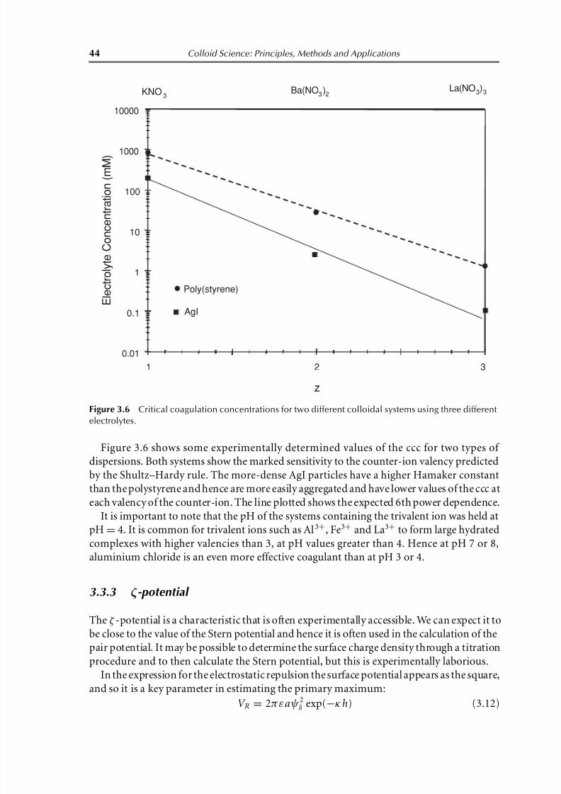
Figure 3.6 Critical coagulation concentrations for two different colloidal systems using three different

electrolytes.

Figure 3.6 shows some experimentally determined values of the ccc for two types of

dispersions. Both systems show the marked sensitivity to the counter-ion valency predicted

by the Shultz–Hardy rule. The more-dense AgI particles have a higher Hamaker constant

than the polystyrene and hence are more easily aggregated and have lower values of the ccc at

each valency of the counter-ion. The line plotted shows the expected 6th power dependence.

It is important to note that the pH of the systems containing the trivalent ion was held at

pH= 4. It is common for trivalent ions such as Al3+, Fe3+ and La3+ to form large hydrated

complexes with higher valencies than 3, at pH values greater than 4. Hence at pH 7 or 8,

aluminium chloride is an even more effective coagulant than at pH 3 or 4.

3.3.3 ζ -potential

The ζ -potential is a characteristic that is often experimentally accessible. We can expect it to

be close to the value of the Stern potential and hence it is often used in the calculation of the

pair potential. It may be possible to determine the surface charge density through a titration

procedure and to then calculate the Stern potential, but this is experimentally laborious.

In the expression for the electrostatic repulsion the surface potential appears as the square,

and so it is a key parameter in estimating the primary maximum:

V R = 2πεa ψ2δ exp(−κh) (3.12)




0

100

200

300

400

500

−1000 10 20 30 40 50

V T

( k B

T )

h (nm)

Figure 3.7 The effect of ζ -potential on the shape of the total interaction potential curve for a polystyrene

latex. From the bottom to top the ζ -potentials are −20 mV, −25 mV, −50 mV and −80 mV.

In the example given in Figure 3.7 for polymer latex particles in 1 mM NaCl, we need a value

in excess of 20 mV to produce a stable dispersion.

When the ζ -potential is−25 mV the value of V max is ∼40k B T . When we double that to

−50 mV we can see that V max ∼ 160k B T . So as expected, since V R is related to the square

of the ζ -potential, a doubling of the ζ -potential leads to a quadrupling of the value of V max.

In this example, when the ζ -potential reduces to less than −20 mV the value of V max

drops below 20k B T and significant aggregation will occur.

3.3.4 Particle size

Both the attractive and repulsive contributions are proportional to the particle radius. At

small sizes the value of V T is directly proportional to the particle size. However, at large sizes

the value of V T has a more complicated variation.

In all cases a larger particle radius leads to a higher energy barrier; in other words,

electrostatic stability increases with increasing particle radius (all other factors remaining

constant). For small particle sizes (<100 nm radius) the primary maximum is directly

proportional to the radius. However, the relationship breaks down at larger sizes and theheight of the primary maximum increases at a lower rate.

The shape of the curve of the attractive interaction is the important point here. Another

feature of this is that for particles with large radii, the attraction often dominates again at

long range giving rise to a secondary minimum at distances of the order of 5–10 nm. This

attraction is manifest as weak but reversible aggregation.

We can make a distinction here between two types of aggregation. Coagulation is the

rapid aggregation that happens in the absence of a primary maximum and leads to a strong

irreversible aggregated structure. Flocculation is a reversible aggregation that occurs in a

secondary minimum as described. Flocculation is reversible on the addition of energy to

the system, usually the application of a shear field by shaking, stirring or other mechanical

processes.




3.4 Kinetics of Coagulation

The rate of coagulation is used either directly or indirectly to determine the ccc. For example

if the rate is monitored, we find that it increases as the electrolyte concentration is increased

until it reaches a plateau value. If we just add particles to different electrolyte solutions in a

series of tubes, then we can check for the onset of aggregation after a fixed time. This may

be 5 min, or we may choose a little longer, but it is still the faster rate that we notice.

As we have already established that electrostatically stabilised dispersions are kinetically

stable and not thermodynamically stable, the key factor is the kinetics. If the rate is so slow

that we do not detect a significant change during our period of use, we would consider that

to be adequately stable.

3.4.1 Diffusion limited rapid coagulation

Recall that the diffusion constant is in terms of the flux through a unit area per second ( J p ):

J p = D 4πr 2dN

dr (3.13)

We can calculate the flow through a spherical surface around a reference particle (see

Figure 3.8). This gives us a differential equation that is easily solved to give the number of

collisions with that reference particle. Of course each particle is itself such a particle and so

the total number of collisions is that for one particle multiplied by the total particle number.

We must divide by 2 as particle A colliding with particle B is the same collision as particle Bcolliding with particle A.

We can allow for the fact that all particles are in motion by using the sum of the diffusion

constants of the two colliding particles. As we are assuming them all to be of the same size,

we multiply by 2. As each collision results in coagulation the coagulation rate is simply the

collision rate.

r

Figure 3.8 Theoretical spherical surface of influence surrounding a reference particle.




φ

0.001 0.01 0.1

H

a l f - l i f e i n s e c o n d s f o r c o a g u l a t i o n

10−6

10−4

10−2

100

102

a = 20 nm

a = 100 nm

a = 500 nm

a = 1000 nm

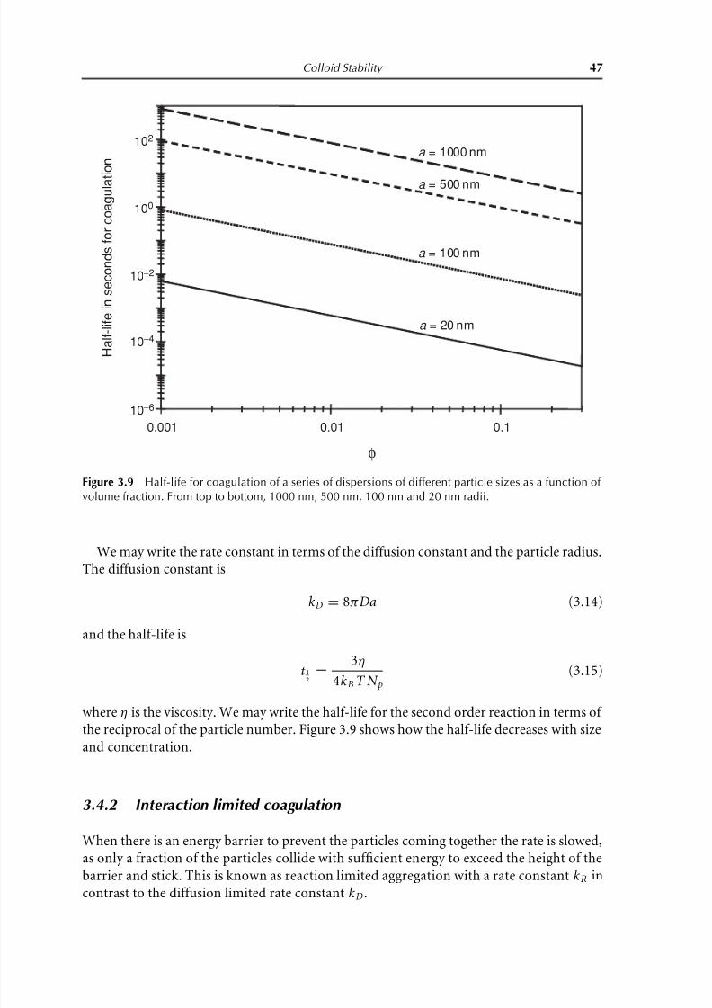
Figure 3.9 Half-life for coagulation of a series of dispersions of different particle sizes as a function of

volume fraction. From top to bottom, 1000 nm, 500 nm, 100 nm and 20 nm radii.

We may write the rate constant in terms of the diffusion constant and the particle radius.

The diffusion constant is

k D = 8πDa (3.14)

and the half-life is

t 12=

3η

4k B T N p(3.15)

where η is the viscosity. We may write the half-life for the second order reaction in terms of the reciprocal of the particle number. Figure 3.9 shows how the half-life decreases with size

and concentration.

3.4.2 Interaction limited coagulation

When there is an energy barrier to prevent the particles coming together the rate is slowed,

as only a fraction of the particles collide with sufficient energy to exceed the height of the

barrier and stick. This is known as reaction limited aggregation with a rate constant k R

in

contrast to the diffusion limited rate constant k D .




Fuchs [8] defined the stability ratio W as the ratio of the rate constants so that the higher

the stability ratio the slower the rate:

W =

k D

k R (3.16)

To a good approximation the reaction limited diffusion rate constant is proportional to the

Boltzmann factor which gives the fraction of particles at any instant with energy in excess

of the primary maximum. The rate of aggregation drops rapidly with the increase in the

energy barrier, so that 10–20k B T gives us reasonable kinetic stability.

Overbeek [4] has shown that a reasonable approximation to the stability ratio is obtained

using the value of the primary maximum:

W =1

2κa

expV max

k B T (3.17)

from which we can show that

k R ≈ 16πκDa 2 exp

−V max

k B T

(3.18)

3.4.3 Experimental determination of the ccc

The ccc is the salt concentration at which there is a change from aggregation which is limitedby the presence of a primary maximum to aggregation which has no barrier. At this point

there is a distinct change in the coagulation rate. Measurement of the coagulation rate can

be made in two ways

r directly – by measuring the number of particles as a function of time by particle counting

(best for large particles) r indirectly – by light scattering (best for small particles).

In each case we are observing the change in the number of aggregates with time. This tells

us about the loss of primary particles from the system.

The simplest experiment is to make up a series of tubes with different electrolyte concen-trations and observe at which concentration aggregation becomes apparent after, say, 5 or

10 min. It can be quantified if the tubes are lightly centrifuged and a spectrophotometer is

used to measure the per cent transmission of the supernatant as a measure of the number

of particles in suspension.

More precise determination can be made if the rate of aggregation itself is measured.

At higher electrolyte concentrations the rate increases to the plateau value (as seen in Fig-

ure 3.10) representing the fast or diffusion limited rate.

Note that the analysis of the rate constant in terms of the diffusion of single particles

is strictly the initial rate. As we progress into the coagulation process the particle number

changes and the mechanism changes to one where the large much less mobile aggregates get

larger by adding singlets. Accurately describing the rates can then be quite complex.




log [NaCl]

l o g k

Rapid coagulation W ~ 1

Slow coagulation

ccc

Figure 3.10 Rate of coagulation against salt concentration indicating the ccc.

3.5 Conclusions

In this chapter we have explored the basic theory surrounding the stability of systems

containing charged colloidal particles. The balance between the van der Waals interaction

and the repulsion between the electrical double layers surrounding charged particles can be

controlled to provide an energetic barrier to the coagulation of particles.We have seen that charge stabilisation can only be effective where significant surface

charge can be achieved and so is normally limited to systems in polar solvents.

The stability achieved is only a kinetic stability to coagulation and in the absence of any

other stabilising mechanism these systems will eventuallycoagulate. However, in the stability

ratio we have a method for evaluating the rate of coagulation compared with the theoretical

rate when there is no barrier to aggregation.

References

1. Hamaker, H.C. (1937) Physica , 4, 1058.

2. Hogg, R., Healey, T.W. and Fuerstenau, D.W. (1966) Trans. Faraday Soc ., 62, 1638.

3. Derjaguin, B.V. and Landau, L. (1941) Acta Physicochim. (URSS), 14, 633.

4. Verwey, E.J. and Overbeek, J.T.G. (1948) Theory of the Stability of Lyophobic Colloids . Elsevier,

Amsterdam.

5. Schulze, J. (1882) pr. Chem., 25, 471.

6. Schulze, J. (1883) pr. Chem., 27, 320.

7. Hardy, W.B. (1900) Proc. R. Soc., 66a, 110.

8. Fuchs, N. (1934) Z. Phys ., 89, 736.

Colloid Stability

Documents

Transcript of Colloid Stability