H.T. HuynhGlenn Research Center, Cleveland, Ohio

Collocation and Galerkin Time-Stepping Methods

NASA/TM—2011-216340

August 2011

https://ntrs.nasa.gov/search.jsp?R=20110014969 2018-07-22T13:00:17+00:00Z

NASA STI Program . . . in Profile

Since its founding, NASA has been dedicated to the advancement of aeronautics and space science. The NASA Scientific and Technical Information (STI) program plays a key part in helping NASA maintain this important role.

The NASA STI Program operates under the auspices of the Agency Chief Information Officer. It collects, organizes, provides for archiving, and disseminates NASA’s STI. The NASA STI program provides access to the NASA Aeronautics and Space Database and its public interface, the NASA Technical Reports Server, thus providing one of the largest collections of aeronautical and space science STI in the world. Results are published in both non-NASA channels and by NASA in the NASA STI Report Series, which includes the following report types: • TECHNICAL PUBLICATION. Reports of

completed research or a major significant phase of research that present the results of NASA programs and include extensive data or theoretical analysis. Includes compilations of significant scientific and technical data and information deemed to be of continuing reference value. NASA counterpart of peer-reviewed formal professional papers but has less stringent limitations on manuscript length and extent of graphic presentations.

• TECHNICAL MEMORANDUM. Scientific

and technical findings that are preliminary or of specialized interest, e.g., quick release reports, working papers, and bibliographies that contain minimal annotation. Does not contain extensive analysis.

• CONTRACTOR REPORT. Scientific and

technical findings by NASA-sponsored contractors and grantees.

• CONFERENCE PUBLICATION. Collected papers from scientific and technical conferences, symposia, seminars, or other meetings sponsored or cosponsored by NASA.

• SPECIAL PUBLICATION. Scientific,

technical, or historical information from NASA programs, projects, and missions, often concerned with subjects having substantial public interest.

• TECHNICAL TRANSLATION. English-

language translations of foreign scientific and technical material pertinent to NASA’s mission.

Specialized services also include creating custom thesauri, building customized databases, organizing and publishing research results.

For more information about the NASA STI program, see the following:

• Access the NASA STI program home page at http://www.sti.nasa.gov

• E-mail your question via the Internet to help@

sti.nasa.gov • Fax your question to the NASA STI Help Desk

at 443–757–5803 • Telephone the NASA STI Help Desk at 443–757–5802 • Write to:

NASA Center for AeroSpace Information (CASI) 7115 Standard Drive Hanover, MD 21076–1320

H.T. HuynhGlenn Research Center, Cleveland, Ohio

Collocation and Galerkin Time-Stepping Methods

NASA/TM—2011-216340

August 2011

National Aeronautics andSpace Administration

Glenn Research Center Cleveland, Ohio 44135

Prepared for the19th Computational Fluid Dynamics Conferencesponsored by the American Institute of Aeronautics and AstronauticsSan Antonio, Texas, June 22–25, 2009

Available from

NASA Center for Aerospace Information7115 Standard DriveHanover, MD 21076–1320

National Technical Information Service5301 Shawnee Road

Alexandria, VA 22312

Available electronically at http://www.sti.nasa.gov

Level of Review: This material has been technically reviewed by technical management.

NASA/TM—2011-216340 1

Collocation and Galerkin Time-Stepping Methods

H.T. Huynh National Aeronautics and Space Administration

Glenn Research Center Cleveland, Ohio 44135

Abstract We study the numerical solutions of ordinary differential equations by one-step methods where the

solution at tn is known and that at tn+1 is to be calculated. The approaches employed are collocation, continuous Galerkin (CG) and discontinuous Galerkin (DG). Relations among these three approaches are established. A quadrature formula using s evaluation points is employed for the Galerkin formulations. We show that with such a quadrature, the CG method is identical to the collocation method using quadrature points as collocation points. Furthermore, if the quadrature formula is the right Radau one (including tn+1), then the DG and CG methods also become identical, and they reduce to the Radau IIA collocation method. In addition, we present a generalization of DG that yields a method identical to CG and collocation with arbitrary collocation points. Thus, the collocation, CG, and generalized DG methods are equivalent, and the latter two methods can be formulated using the differential instead of integral equation. Finally, all schemes discussed can be cast as s-stage implicit Runge-Kutta methods.

1.0 Introduction Collocation is an idea widely applicable to numerical analysis. In the case of numerical solutions for

differential equations (or time-stepping schemes), for the one-step methods where the data un at tn is known and the solution un+1 at tn+1 is to be calculated, the collocation approach can be formulated as follows (e.g., Hairer, Norsett, and Wanner 1987, Lambert 1991). The solution is first approximated on [tn, tn+1] by a polynomial P of degree s (for s-stage) interpolating the solution values at s points on [tn, tn+1] called collocation points together with the value un at tn. The polynomial P is determined by requiring that it satisfies the differential equation at the s collocation points. The solution un+1 is given by P(tn+1). For these methods, their accuracy and stability are determined by the choice of collocation points. For example, if the s points are chosen to be the Gauss, Radau, or Lobatto points, then the resulting method is accurate to order 2s, 2s – 1, or 2s – 2, respectively. Collocation methods were studied in (Cooper 1968, Axelsson 1969). Wright (1970) showed that the collocation process leads to an s-stage implicit Runge-Kutta (IRK) method. His proof will be reproduced and utilized here.

The Galerkin method was introduced in 1915 for the elastic equilibrium of rods and thin plates (Fletcher 1984). It was employed to solve ordinary differential equations by Hulme (1972). An introduction to both continuous Galerkin (CG) and discontinuous Galerkin (DG) methods for differential equations can be found in (Eriksson et al. 1996). The CG method seeks to approximate the solution by a continuous function which, on each interval [tn, tn+1], is a polynomial of degree s. This polynomial is determined by requiring that on [tn, tn+1], the weak form of the differential equation holds for all test functions that are polynomials of degree s vanishing at tn. Hulme (1972) showed that if an s-point quadrature formula is employed, then the resulting CG method is equivalent to a collocation method provided that the step size is bounded by certain norms to ensure the uniqueness of both solutions—a condition which will be removed here. (Solution uniqueness is not always available, e.g., for the three-dimensional Navier-Stokes equations, the problem of existence and uniqueness of the solution is still open.)

The discontinuous Galerkin method (DG) is currently popular for the spatial discretization of conservation laws (see the review paper by Cockburn, Karniadakis, and Shu, 2000). Formulated for differential equations by LeSaint and Raviart (1974), the DG method seeks to approximate the solution by a function, which can be discontinuous across tn, and is a polynomial of degree k on each [tn, tn+1]. At each tn where the solution is discontinuous, the value chosen is that just to its left—for conservation laws, such

NASA/TM—2011-216340 2

a choice is called ‘upwinding’; it serves the purpose of adding numerical dissipation and results in a more stable method. Here, after an integration by parts, this upwind value is employed to evaluate the boundary term. The polynomial of degree k representing the solution is determined by requiring that on [tn, tn+1], the weak form of the differential equation (after the integration by parts) holds for all test functions that are polynomials of degree k. Using a quadrature formula with k + 1 evaluations including an evaluation at the left boundary tn, LeSaint and Raviart showed that the DG formulation results in a (k + 1)-stage implicit Runge-Kutta (IRK) method accurate to order 2k +1 or less. In addition, they proved the strong A-stability property (see also Bauer 1995). The method was generalized by employing the boundary values to the right of tn+1 in (Delfour, Hager, and Trochu 1981). The relation between DG and collocation methods, however, has not been established. On a different but related subject, it was proven in (Adjerid et al. 2002) that for conservation laws, the DG method is superconvergent to order 2k +1 at the “downwind” boundary of each cell. Concerning the basic formulation, it was shown in (Huynh 2007) that for conservation laws (on a quadrilateral mesh), the DG method can be formulated using the differential form, and the result is a simple and economical algorithm.

In this paper, we first prove that if an s-point quadrature formula is employed, then the CG method using polynomials of degree s is identical to the collocation method using the s quadrature points as collocation points; in other words, the condition on the step size being small enough in (Hulme 1972) is removed. Our proof is constructive; in addition, it shows the equivalence of the integral and differential forms: with appropriate choices of basis functions, one set for the space of trial solutions and another for the space of test functions, the CG (integral) formulation is shown to result in a collocation (differential) formulation. In contrast, a typical CG formulation employs (essentially) the same basis functions for the trial and test spaces. Next, we show that if the quadrature formula is the right Radau one (including the right boundary tn+1), then the DG and CG methods also become identical, and they reduce to a collocation method called Radau IIA. Compared to the proof of the fact that the DG method can be cast in the form of IRK by LeSaint and Raviart, our proof is more direct and leads to a specific member of the IRK class, namely, Radau IIA. In addition, it results in a formulation of DG using the differential instead of integral equation. Such a formulation can simplify the time discretization of the space-time DG scheme (for standard space-time DG methods, see (Van der Vegt and Van der Ven 2002)). Finally, we generalize the DG formulation in a manner that the resulting method becomes identical to CG. Our approach to this generalization does not involve the value to the right of tn+1; therefore, it is simpler than the approach of Delfour, Hager, and Trochu (1981).

Most papers on this subject are written in a highly concise manner. Often, readers can find the motivation and meaning of a technique or an equation only after plowing through complicated algebraic expressions. Such conciseness may make for an elegant style; however, it can sometimes cause misunderstanding. For example, in (Delfour et al. 1981), it was stated that their generalized DG method has the property of “superconvergence of order 2k +1” where k is the degree of the discontinuous piecewise polynomial. Concerning the CG method discussed by Hulme (1972), they stated: “Note, however, that these continuous approximations have order 2k at the mesh points instead of 2k +1”. It will be shown here that the CG method is, in fact, more accurate than DG: if s is the number of stages for the resulting IRK method, then, concerning highest attainable accuracy, CG is of order 2s, whereas DG, order 2s – 1. To put it differently, for highest accuracy, CG corresponds to the Gauss quadrature, whereas DG, the right Radau one; as a result, CG is more accurate than DG. Note that for stiff problems, an even more critical criterion is stability, and here, the DG or right Radau collocation method is more advantageous.

This paper is written in an expository manner since several different methods are involved, and a typical reader may be unfamiliar with one or more of them. Another goal of the expository style is to avoid misunderstanding. The paper is organized as follows: the collocation method is discussed in Section 2.0; CG in Section 3.0; and DG in Section 4.0. A brief review of Legendre and Radau polynomials and a few examples of collocation methods can be found in the Appendices.

We now set up the problem and introduce notations and techniques common to all methods. Note that the methods discussed here can be applied to systems of equations; for simplicity of notation, we deal only with the scalar case. Consider the ordinary differential equation (ODE)

NASA/TM—2011-216340 3

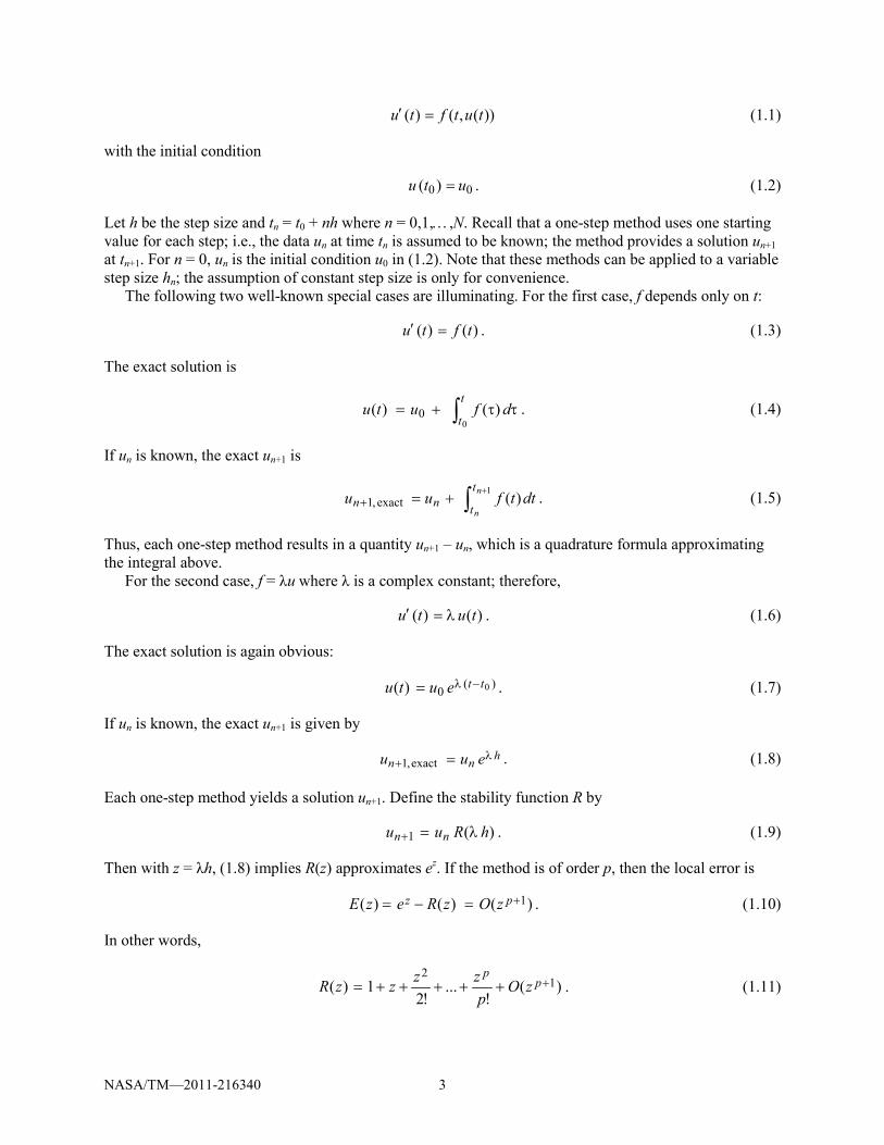
))(,()( tutftu =′ (1.1)

with the initial condition

00)( utu = . (1.2)

Let h be the step size and tn = t0 + nh where n = 0,1,…,N. Recall that a one-step method uses one starting value for each step; i.e., the data un at time tn is assumed to be known; the method provides a solution un+1 at tn+1. For n = 0, un is the initial condition u0 in (1.2). Note that these methods can be applied to a variable step size hn; the assumption of constant step size is only for convenience.

The following two well-known special cases are illuminating. For the first case, f depends only on t:

)()( tftu =′ . (1.3)

The exact solution is

∫ ττ+=t

tdfutu

0)()( 0 . (1.4)

If un is known, the exact un+1 is

∫+

+=+1 )(exact,1

n

n

t

tnn dttfuu . (1.5)

Thus, each one-step method results in a quantity un+1 – un, which is a quadrature formula approximating the integral above.

For the second case, f = λu where λ is a complex constant; therefore,

)()( tutu λ=′ . (1.6)

The exact solution is again obvious:

)(0 0)( tteutu −λ= . (1.7)

If un is known, the exact un+1 is given by

hnn euu λ+ =exact,1 . (1.8)

Each one-step method yields a solution un+1. Define the stability function R by

)(1 hRuu nn λ=+ . (1.9)

Then with z = λh, (1.8) implies R(z) approximates ez. If the method is of order p, then the local error is

)()()( 1+=−= pz zOzRezE . (1.10)

In other words,

)(!

...!2

1)( 12

++++++= pp

zOpzzzzR . (1.11)

NASA/TM—2011-216340 4

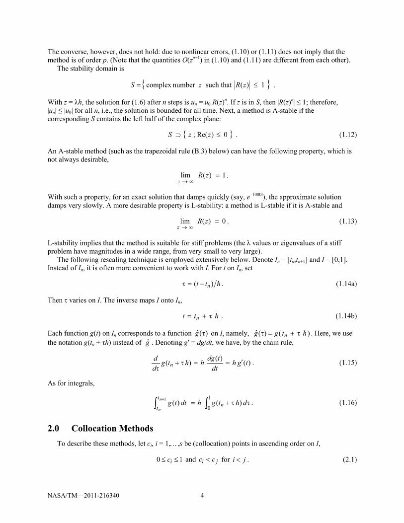
The converse, however, does not hold: due to nonlinear errors, (1.10) or (1.11) does not imply that the method is of order p. (Note that the quantities O(zp+1) in (1.10) and (1.11) are different from each other).

The stability domain is

{ }1)(such thatnumber complex ≤= zRzS .

With z = λh, the solution for (1.6) after n steps is un = u0 R(z)n. If z is in S, then |R(z)n| ≤ 1; therefore, |un| ≤ |u0| for all n, i.e., the solution is bounded for all time. Next, a method is A-stable if the corresponding S contains the left half of the complex plane:

{ }0)Re(; ≤⊃ zzS . (1.12)

An A-stable method (such as the trapezoidal rule (B.3) below) can have the following property, which is not always desirable,

1)(lim =∞→

zRz

.

With such a property, for an exact solution that damps quickly (say, e–1000t), the approximate solution damps very slowly. A more desirable property is L-stability: a method is L-stable if it is A-stable and

0)(lim =∞→

zRz

. (1.13)

L-stability implies that the method is suitable for stiff problems (the λ values or eigenvalues of a stiff problem have magnitudes in a wide range, from very small to very large).

The following rescaling technique is employed extensively below. Denote In = [tn,tn+1] and I = [0,1]. Instead of In, it is often more convenient to work with I. For t on In, set

htt n )( −=τ . (1.14a)

Then τ varies on I. The inverse maps I onto In,

htt n τ+= . (1.14b)

Each function g(t) on In corresponds to a function )(ˆ τg on I, namely, )()(ˆ htgg n τ+=τ . Here, we use the notation g(tn + τh) instead of g . Denoting g′ = dg/dt, we have, by the chain rule,

)()()( tghdt

tdghhtgdd

n ′==τ+τ

. (1.15)

As for integrals,

ττ+= ∫∫+ 1

0)()(1 dhtghtdtg n

t

t

n

n. (1.16)

2.0 Collocation Methods To describe these methods, let ci, i = 1,…,s be (collocation) points in ascending order on I,

10 ≤≤ ic and ji cc < for ji < . (2.1)

NASA/TM—2011-216340 5

Let the collocation points on In be defined by

hctt inin +=, . (2.2)

Suppose, for the moment, the solution values un,i at tn,i, i = 1,…,s, are known. These s values together with the value un at tn determine a polynomial P = P(t) of degree s (the case c1 = 0 will be discussed later),

nn utP =)( (2.3)

and, for i = 1,…,s,

inin utP ,, )( = . (2.4)

The quantities P′(tn,i) = (dP/dt)(tn,i) and f (tn,i,un,i) can then be evaluated for i = 1,…,s. The collocation method seeks a polynomial P that satisfies the following implicit equations: for i = 1,…,s,

))(,(),()( ,,,,, ininininin tPtfutftP ==′ (2.5)

Once P is determined, the solution at tn+1 is given by

)( 11 ++ = nn tPu . (2.6)

Two remarks are in order. First, the approximating polynomials for u and f of the ODE are of different degrees. Indeed, if u is approximated by P of degree s, then u′ is approximated by P′ of degree s – 1. Since u′ = f, we wish to approximate f by a polynomial of degree s – 1. For the collocation method, this polynomial is determined by the values of f at tn,1,…,tn,s (and not the value at tn). As an example, for the equation u′ = λu, the function u of the left hand side is approximated by P, whereas, u of the right hand side, by the values at the collocation points tn,1,…,tn,s (a polynomial of degree s – 1).

The second remark concerns the case c1 = 0. Here, the derivative P′(tn,1) = P′(tn) = f (tn,un) can be calculated explicitly. Therefore, P is determined by (2.5) with i = 2,…,s and

nn utP =)( and ),()( nnn utftP =′ . (2.7)

2.1 Collocation and Implicit Runge-Kutta (IRK) Methods

It was shown by Wright (1970) that the above collocation method results in an s-stage IRK method. The proof of this fact (Lambert 1991) is reproduced below since it will be employed for our proof of equivalence between CG and collocation methods. It amounts to expressing P′ in terms of certain basis functions and then integrating P′ to obtain P in IRK form.

Consider the s collocation points c1,…,cs on [0,1]. The values (of a function) at these points determine a polynomial of degree s – 1. With i fixed, 1 ≤ i ≤ s, let Li(τ) be the Lagrange polynomial of degree s – 1 defined by Li(cj) = δij for j = 1,…,s; i.e., Li takes value 1 at τ = ci and 0 at all other cj, j ≠ i (see Fig. 2.1),

∏≠= −

−τ=τ

s

ijj ji

ji cc

cL

,1)( . (2.8)

Then Li, 1 ≤ i ≤ s, form a basis for the space of polynomials of degree s – 1 on [0,1].

NASA/TM—2011-216340 6

(a)

(b)

Figure 2.1.—(a) Functions Lj, j = 1,2,3 for the case of 3 Gauss points (s = 3) as collocation points on the interval I = [0,1]. (b) The same functions for the case of 2 right Radau points (c2 = 1).

For i = 1,…,s, set

),( ,, inini utfk = . (2.9)

Next, observe that P′ = dP/dt is a polynomial of degree s – 1. Using j for the index instead of i (the reason for this switch will be clear in (2.11)), since P′ interpolates the s data points (tn + cjh,kj),

∑ =τ=τ+′ s

j jjn kLhtP1

)()( . (2.10)

Concerning the above left hand side, with t = tn + τh, we have

)()()()(0 nin

hct

t

cn tPhctPdttPdhtPh in

n

i−+=′=ττ+′ ∫∫

+.

Equation (2.10) then implies, for the i-th stage,

jsj

cjnin kdLhtPhctP i∑ ∫=

ττ=−+

1 0)()()( . (2.11)

As for the solution un+1,

jsj jnnnn kdLhtPhtPuu ∑ ∫=+

ττ=−+=−

1

1

01 )()()( . (2.12)

Motivated by (2.11), set

∫ ττ=ic

jij dLa0

)( , (2.13)

and, by (2.12), set

∫ ττ=1

0)( dLb jj . (2.14)

Then, with un,j = P(tn,j) and kj = f (tn,j, un,j), (2.11) implies the following IRK form of the collocation method: for i = 1,…,s,

0.2 0.4 0.6 0.8 1

-0.5

0.5

1

1.5

0.2 0.4 0.6 0.8 1

-0.5

0.5

1

1.5

1L

2L 1L

2L τ τ 1c 3c

1c 2c 2c

3L

NASA/TM—2011-216340 7

jsj ijnin kahuu ∑ =

+=1, . (2.15)

After obtaining un,i (and ki) by solving the above system of s implicit equations, the solution is given by

jsj jnn kbhuu ∑ =+ +=

11 . (2.16)

This completes the proof. The Butcher array of an IRK method consists of ci, aij, and bj arranged as follows

1c 11a sa1

sc 1sa ssa

1b sb

Here, for each i-th row, aij, j = 1,…,s are the weights of a quadrature formula as will be shown in (2.18).

Note that if c1 = 0, then tn,1 = tn, un,1 = un, and a1j = 0 for all j; in other words, the first row of the Butcher array is identically zero. In addition, the quantity k1 = f (tn,un) can be calculated explicitly. Since un,1 = un is known, (2.15) for i = 2,…,s then yields the equations to calculate un,2,…,un,s.

Concerning the stability function for the IRK method, define the s×s matrices A = [aij] and I = identity matrix, column vectors of s entries b = [b1,…,bs]T and e = [1,1,…,1]T where the superscript T stands for transpose, and det = determinant. Then, for the IRK method, the stability function R can be calculated by one of the following two formulas (e.g., Lambert 1991)

ezzbzR T 1)(1)( −−+= AI

or

][det

]1[det)(AI

Az

zebzzRT

−+−

= .

2.2 Quadratures Associated with IRK Method

The above IRK method relates to quadrature formulas as follows. By (2.16) and the definition of kj,

jnsj jnn ubhuu ,11 ′=− ∑ =+ .

The corresponding quadrature formula is, for any continuous function v on I = [0,1],

)()(1

1

0 jsj j cvbdv ∑∫ =

≈ττ . (2.17)

Here, bj are the weights given in (2.14), and the collocation points cj are the evaluation points. Similarly, by (2.15),

jnsj ijnin uahuu ,1, ′=− ∑ =

.

NASA/TM—2011-216340 8

The corresponding quadrature formula is

)()(10 j

sj ij

ccvadvi ∑∫ =

≈ττ . (2.18)

Here, we use the s collocation points on [0,1] to evaluate the integral from 0 to ci. An observation concerning accuracy of these quadratures is in order. With appropriate choice of

evaluation points on I, formula (2.17) has a degree of precision of up to 2s – 1. (Recall that a quadrature is of degree of precision m if it is exact for polynomials of degree m or less.) Formula (2.18) for the stages, however, has a degree of precision no higher than s – 1 since special points (say, Gauss points) on [0,1] are generally not special on [0,ci]. For example, if we use 2 Gauss points on [0,1] as collocation points, then the degree of precision for (2.17) is 3, but that for (2.18) is only 1. As will be shown, the resulting collocation method is of order 4.

2.3 Basis Functions jL~

We next introduce the basis functions jL~ , which will be employed in the proof of equivalence between the collocation and CG methods. With t = tn + τh, similar to (2.11), by (2.10),

jsj jn kdLhtPtP ∑ ∫=

ξ

ττ=−

1 0)()()( . (2.19)

Denote, for j = 1,…,s,

∫τ

ξξ=τ0

)()(~ dLL jj . (2.20)

Then jL~ is of degree s since Lj is of degree s – 1. Some additional noteworthy properties of jL~ are:

jj LdLd =τ/~ ; (2.21a)

in addition,

jjijijj bLacLL === )1(~ and,)(~,0)0(~ ; (2.21b)

moreover, since 11

=∑ =sj jL ,

τ=τ∑ =)(~

1sj jL . (2.22)

Next, by (2.19),

∑ =τ=−τ+=−

sj jjnnn LkhtPhtPtPtP

1)(~)()()()( . (2.23)

NASA/TM—2011-216340 9

(a)

(b)

Figure 2.2.—(a) Functions jL~ j = 1,2,3 for the case of 3 Gauss points on I = [0,1]. Note that )(/)(~τ=ττ jj LdLd ;

therefore, the graph of jL~ has slope 1 at cj and slope 0 at all other ci as can be seen by the slopes at the dots. (b) Functions jL~ for the case of 2 (right) Radau points.

For convenience, set

1~0 =L (2.24a)

and

huhtPk nn //)(0 == . (2.24b)

Then 00~)( LkhtP n = , and (2.23) can be expressed as

∑ =τ=τ+

sj jjn LkhhtP

0)(~)( . (2.25)

Observe that jL~ , j = 0,…,s, are s + 1 polynomials of degree no higher than s. We will show that they are linearly independent; thus, they form a basis for the space of polynomials of degree s or less. That is, we wish to show that if

0~0

=α∑ =sj jj L , (2.26)

then

0=α j for sj ...,,0= . (2.27)

To this end, observe that (2.26) implies 0)0(~0

=α∑ =sj jj L . Since 0)0(~

=jL for j = 1,…,s, we have

0)0(~00 =α L . By definition, 1~

0 =L ; as a result,

00 =α . (2.28)

Equation (2.26) then takes the form

0~1

=α∑ =sj jj L . (2.29)

Note the starting value of 1 for j. Differentiating the above, we have

0.2 0.4 0.6 0.8 1

0.1

0.2

0.3

0.4

0.2 0.4 0.6 0.8 1

0.2

0.4

0.6

1~L

2

~L 1

~L

2~L

τ τ 3

~L

NASA/TM—2011-216340 10

01

=α∑ =sj jj L .

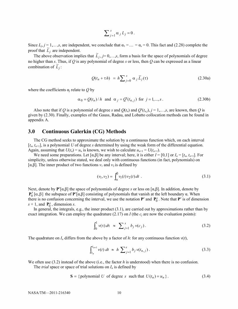
Since Lj, j = 1,…,s, are independent, we conclude that α1 = … = αs = 0. This fact and (2.28) complete the proof that jL~ are independent.

The above observation implies that jL~ , j= 0,…,s, form a basis for the space of polynomials of degree no higher than s. Thus, if Q is any polynomial of degree s or less, then Q can be expressed as a linear combination of jL~ :

∑ =τα=τ+

sj jjn LhhtQ

0)(~)( (2.30a)

where the coefficients αj relate to Q by

htQ n /)(0 =α and )( , jnj tQ′=α for sj ...,,1= . (2.30b)

Also note that if Q is a polynomial of degree s and Q(tn) and Q′(tn,j), j = 1,…,s, are known, then Q is given by (2.30). Finally, examples of the Gauss, Radau, and Lobatto collocation methods can be found in appendix A.

3.0 Continuous Galerkin (CG) Methods The CG method seeks to approximate the solution by a continuous function which, on each interval

[tn, tn+1], is a polynomial U of degree s determined by using the weak form of the differential equation. Again, assuming that U(tn) = un is known, we wish to calculate un+1 = U(tn+1).

We need some preparations. Let [α,β] be any interval; here, it is either I = [0,1] or In = [tn, tn+1]. For simplicity, unless otherwise stated, we deal only with continuous functions (in fact, polynomials) on [α,β]. The inner product of two functions v1 and v2 is defined by

tdtvtvvv ∫β

α= )()(),( 2121 . (3.1)

Next, denote by Ps[α,β] the space of polynomials of degree s or less on [α,β]. In addition, denote by ],[0 βαsP the subspace of Ps[α,β] consisting of polynomials that vanish at the left boundary α. When

there is no confusion concerning the interval, we use the notation Ps and s0P . Note that Ps is of dimension

s + 1, and s0P , dimension s.

In general, the integrals, e.g., the inner product (3.1), are carried out by approximations rather than by exact integration. We can employ the quadrature (2.17) on I (the cj are now the evaluation points):

)()(1

1

0 jsj j cvbdv ∑∫ =

≈ττ . (3.2)

The quadrature on In differs from the above by a factor of h: for any continuous function v(t),

∑∫ =≈

+ sj jnj

t

ttvbhtdtvn

n 1 , )()(1 . (3.3)

We often use (3.2) instead of the above (i.e., the factor h is understood) when there is no confusion. The trial space or space of trial solutions on In is defined by

})( such that degree of polynomial{ nn utUsU ==S . (3.4)

NASA/TM—2011-216340 11

In spite of its name, S is in fact not a space, but is a hyperplane in Ps[tn, tn+1]. A test space or a space of test functions on In, commonly denoted by V, is a subspace of Ps which has

dimension s. Among the most commonly used test spaces is the space consisting of polynomials that satisfy the homogeneous boundary condition at tn

}0)( such that degree of { == ntvsvV , (3.5)

i.e., s0PV = . Note that if U is in S, then U – un is an element of the above V.

Next, the weak form of the equation u′ = f can be written formally as

),(),( vfvu =′ . (3.6)

The CG method seeks a solution U in the trial space S that satisfies, for all v in the test space V,

),(),( vfvU =′ . (3.7)

In other words, the projection of U′ and f (t,U(t)) onto V are the same. We now show that the test space, as opposed to the case of trial space, must be a subspace, and it must

have dimension s. Indeed, first, suppose (3.7) holds for functions v1 and v2 (which take the place of v). Let α and β be real numbers. Then, one can easily verify that (U′, αv1 + βv2) = (f, αv1 + βv2); thus, the test space must form a subspace. Next, since U is of degree s, and one condition is known, namely, U(tn) = un, s conditions remain to be determined. Therefore, the test space must be of dimension s.

We next discuss the choice of test spaces. Instead of solving for U, we can solve for U – un. Since U – un is in V, and V defined by (3.5) has the correct dimension, it is sensible to use V as a test space.

The following argument results in another choice of test space. Since U′ is of degree s – 1, for the two sides of (3.7) to match, we should approximate f by a polynomial also of degree s – 1. Such an approximation can be obtained by the projection of f on Ps–1. For this projection to be identical to U′, it suffices to require that (3.7) holds for all v in Ps–1, i.e., the test space be Ps–1. It was observed in (Fletcher 1984) and also in (Eriksson et al. 1996) that this test space yields a more accurate solution than the test space s

0P . We will show in (3.34) below that with the quadrature (3.2), or equivalently, (3.3), the two test spaces s

0PV = and V = Ps–1 yield identical results. The following conclusion can then be drawn: for the CG formulation with the test space s

0PV = , the method using Gauss quadrature is more accurate than that using exact integration. (This fact is contrary to the common belief that more accurate integration formulas yield more accurate solutions.)

(a)

(b)

Figure 3.1.—(a) Basis functions φj j = 0,…,3 for the case of 3 Gauss points on I = [0,1]. (b) Basis functions φ0, φ1, and φ2 for the case of 2 right Radau points. Note that φ1,…, φs form a basis for s

0P .

0.2 0.4 0.6 0.8 1

-1

-0.5

0.5

1

1.5

0.2 0.4 0.6 0.8 1-0.2

0.2

0.4

0.6

0.8

1

1φ

0φ

2φ τ

τ

1φ 2φ 3φ 0φ

NASA/TM—2011-216340 12

In addition to jL~ defined by (2.20), we will need the following basis for Ps. On I, assuming c1 > 0, set

00 =c . (3.8)

Then, c0 > c1 > …. cs ≤ 1. Let φ0,…, φs be the corresponding basis functions: for each j,

∏≠= −

−τ=τφ

s

jii ij

ij cc

c

,0)( . (3.9)

That is, φj(ci) = δij as shown in Figure 3.1. (Note that the definition of Li in (2.8) is different from the current definition in that it does not include c0).

Since φ0(0) = 1, we can employ φ0 to deal with the boundary condition at tn. For all j ≥ 1, φj(0) = 0; as a consequence, φ1,…, φs form a basis for s

0P . Also note that in the case of s Gauss points, φ0 defined above is identical to the Legendre polynomial of degree s on I; in the case of right Radau points, it is identical to the Radau polynomial (see Appendix). In the case of Lobatto points, however, φ0 is not the Lobatto polynomial; this case corresponds to c1 = 0 and will be discussed later.

3.1 CG and Collocation Methods

We claim that if the quadrature formula (3.2) is employed to evaluate the inner product, then the resulting CG method is identical to the collocation method with quadrature points as collocation points.

To prove the above claim, we will start with the CG solution U and show that it can be expressed in collocation form. The key ingredient of the proof is the choice of s

jjL 0}~{ = defined by (2.20) as a basis for S and s

jj 1}{ =φ defined by (3.9) as a basis for s0PV = . Since U – un is in V, and s

jjL 1}~{ = is a basis for V, U – un can be expressed in terms of these basis functions:

∑ =τ=−τ+

sj jjnn LdhuhtU

1)(~)( . (3.10)

As discussed in (2.30), dj and U are related by, for j = 1,…,s,

)( , jnj tUd ′= . (3.11)

We wish to show, by using the weak form (3.7), that dj = f (tn,j,U(tn,j)). To this end, because jj LdLd =τ/~ , by differentiating (3.10) and employing the chain rule,

∑ =τ=τ+′ s

j jjn LdhtU1

)()( . (3.12)

Next, recall that U is a CG solution. Noting that φ1,…,φs form a basis for V, they can serve as test functions: for i = 1,…,s,

),(),( ii fU φ=φ′ . (3.13)

We will show that under the quadrature rule, the left hand side above yields U′(tn,i), and the right hand side, f (tn,i, U(tn,i)). Indeed, by (3.12),

),(),(1 i

sj jji LdU φ=φ′ ∑ =

. (3.14)

NASA/TM—2011-216340 13

When the inner product is evaluated by quadrature (3.2), we use the notation (.,.)q, e.g.,

∑ ==

si iiiq cwcvbwv

1)()(),( .

In (3.14), Lj vanishes at all collocation points except at cj, and φi vanishes at all collocation points except at ci. Consequently, the only nonzero term for the sum is di(Li,φi). Since Li(ci) = φi(ci) = 1, employing the quadrature rule, (3.14) implies

iiqi dbU =φ′ ),( . (3.15)

Concerning the right hand side of (3.13), under the quadrature rule, only the values of f at the quadrature points are needed. Since fφi takes on the value f (tn,i,U(tn,i)) at τ = ci and the value 0 at all other cj,

))(,(),( ,, ininiqi tUtfbf =φ . (3.16)

Again, under the quadrature rule, by (3.15) and (3.16), equation (3.13) implies

))(,( ,, inini tUtfd = .

From the above and (3.11), for i = 1,…,s,

))(,()( ,,, ininin tUtftU =′. (3.17)

That is, U plays the role of P in the definition of the collocation method (2.23). This completes the proof.

3.2 Standard CG Method (Via Basis Functions)

In (3.7) above, the CG method is formulated via trial and test spaces. It can also be formulated via basis functions (Hulme 1972, Delfour et al. 1981). This formulation is presented here with more explanations and will be employed later in (3.35) to (3.45). Let φ0,…,φs be a set of basis functions for Ps[0,1] with the following properties. First,

1)0(0 =ϕ (3.18)

so that φ0 can deal with the boundary condition at tn. Next, for j = 1,….,s,

0)0( =ϕ j (3.19)

so that φ1,…,φs form a basis for s0P . Note that jL~ defined by (2.20) and (2.24a) and φj by (3.9) possess

these properties. Set

hud n=0 . (3.20)

Then the trial solution U of (3.4) can be written as

∑ =τϕ=τ+

sj jjn dhhtU

0)()( (3.21)

where d0 is given by (3.20) and d1,…,ds remain to be determined. Taking d/dτ of the above,

NASA/TM—2011-216340 14

∑ =ττϕ=τ+′ s

j jjn dddhtU0

/)()( . (3.22)

Using the test function v = φi where i = 1,…,s, defined by (3.9) (these φi form a basis for V), the weak form (3.7) implies

),()/,(0

fddd ijsj ji ϕ=τϕϕ∑ =

. (3.23)

We thus obtain s implicit equations (since f also depends on di) for s unknowns d1,…,ds.

Note that in general, the expression

ϕ∑ =

)(,0

tdtf sj jj , which depends on the unknowns dj, can be

complicated; as a result, evaluating (φi,f) via exact integration may become difficult. It is often more convenient to evaluate the inner product by a quadrature formula employing only the values f (tn,j,U(tn,j)) at the quadrature points.

3.3 Equivalence of Collocation and CG Methods Via Approximating the Dirac Delta Function

If we use the Dirac delta function, the proof of this equivalence is shortened considerably. The basic idea is that on Ps with an inner product by quadrature (3.2), the Dirac delta function δi has the same effect as φi/bi where φi is the basis function given by (3.9) and bi is the quadrature weight. Indeed, on I = [0,1], let δi be the Dirac delta function at ci defined by, for any v in Ps,

)(),( ii cvv =δ . (3.24)

Using the quadrature rule (3.2), again for any v in Ps,

),()()/,( iiqii vcvbv δ==φ . (3.25)

That is, concerning the inner product on Ps via the quadrature rule, we have

iii b δ=φ / . (3.26)

The collocation method (2.5), with P defined by (2.3) and (2.4), can be written as

),(),( ii fP δ=δ′ . (3.27)

Therefore, by (3.25), for i = 1,…,s,

qiqi fP ),(),( φ=φ′ . (3.28)

The above is the CG form (3.13) with the inner product evaluated by the quadrature (3.2) and U replaced by P.

Note that for the above argument to hold, φi is required to be of degree s and thus, is defined by s + 1 conditions, but only the s values of φi at the collocation points are needed in the above proof. The extra condition can be arbitrary (i.e., the condition φi(0) = 0 is not required) as discussed further in (3.33) below.

NASA/TM—2011-216340 15

3.4 The Case c1 = 0 (and c2 > 0)

Examples for this case are the Lobatto and the left Radau quadrature points. Via the collocation approach, as discussed in (2.7), for this case, in addition to the boundary value un, the derivative

),( nnn uxfu =′ is also known (easily evaluated). Concerning the CG approach, it needs to be modified to incorporate the condition that nu′ is known. To this end, the trial space is defined as

)},( and)( such that degree of polynomial{ nnnnn uxfUutUsU =′= . (3.29)

This trial space is of dimension s – 1. The test space can be modified accordingly:

}0)( and0)( such that degree of { =′= nn tvtvsv . (3.30)

This space is also of dimension s – 1. For the case c1 = 0, the CG method seeks a solution U in the trial space (3.29) that satisfies, for all v in the test space (3.30),

),(),( vfvU =′ .

Next, the definition of jL~ in (2.20) remains valid. In addition, the definition of the basis functions φj in (3.9), except for φ0 and φ1, also remains valid. Since c0 = c1 = 0, to modify φ0, we define it to be a polynomial of degree s such that

1)0(0 =φ , 0)0(0 =′φ , and 0)(0 =φ ic for si ...,,2= . (3.31a)

That is

∏=

τ−τ−=τφ

s

i i

ic

ca2

0 )1()(

where (3.31b)

)0(2

′

τ−= ∏

=

s

i i

ic

ca .

As for φ1, it is defined to be a polynomial of degree s such that

0)0(1 =φ , 1)0(1 =′φ , and 0)(1 =φ ic for si ...,,2= . (3.32a)

That is

∏=

τ−τ=τφ

s

i i

ic

c

21 )( . (3.32b)

Note that φ0 serves the purpose of matching the value un, and φ1, the slope ),( nnn utfu =′ . The claim of equivalence between CG and collocation methods still holds when c1 = 0. The proof,

which employs the basis functions φ2,…,φs for the test space (3.30), and the basis functions jL~ for the trial space (3.29), is essentially the same as that of the case c1 > 0 and is omitted.

NASA/TM—2011-216340 16

(a)

(b)

Figure 3.2.—(a) Basis functions 30 φφ ...,, for the case of 3 Lobatto points. (b) Basis functions 10 φφ , , and 2φ for the case of 2 left Radau points. Note that sφφ ...,,2 form a basis for the test space defined in (3.30).

3.5 Test Spaces

We claim that using quadrature (3.2) with evaluation points ci’s, the test spaces Ps–1 and s0P (or V)

yield identical results. The reason is that on Ps with such a quadrature, as far as the inner product is concerned, φi defined by (3.9) has the same effect as Li defined by (2.8) for i = 1,…,s. Indeed, for any continuous function v, with i varies between 1 and s,

)(),(),(),( iiqiiqiqi cvbbvLvv =δ==φ . (3.33)

Thus, if U is a solution of the standard CG method, then since φi is in the test space s0P , (U′,φi)q = (f,φi)q.

As shown above, we can replace φi by Li,

qiqi LfLU ),(),( =′ . (3.34)

Noting that Li, i = 1,…,s form a basis for Ps–1, the claim follows. Readers who are interested only in the main results can omit the rest of this section with no loss of

continuity.

3.6 A Dilemma

The question then is: What causes the difference between the established fact that the test space Ps–1 yields a more accurate solution than the test space s

0P and the above claim that under the quadrature rule, the test spaces Ps–1 and s

0P yield identical results? To answer this question, we need to derive the solutions using exact integration. This derivation is similar to that in (Fletcher 1984); the key difference, however, is that instead of u′ = u, we use the equation

uu λ=′ . (3.35)

As a consequence, we can study not only which test space yields a more accurate numerical solution, but also the stability as well as order of accuracy of the corresponding method. We will show that with s

0P as the test space, an appropriate quadrature formula results in a method more accurate than that by exact integration. In other words, such a quadrature provides the cancellation needed for high accuracy whereas, with exact integration, the cancellation no longer occurs. This observation contrasts the common belief that a more accurate integration procedure results in a solution with better accuracy.

To solve the above ODE, consider the following basis functions for Ps[0,1]

sjjj ...,,0, =τ=ϕ . (3.36)

0.2 0.4 0.6 0.8 1

-0.4

-0.2

0.2

0.4

0.6

0.8

1

0.2 0.4 0.6 0.8 1

-0.5

0.5

1

1.5

1φ

0φ 2φ

τ τ 1φ

2φ 3φ 0φ

NASA/TM—2011-216340 17

Clearly, φj(0) = 0 for j = 1,…,s, and φ1,…, φs form a basis for VP =s0 . Next, set

hud n=0 (3.37a)

and

∑ =τϕ=

sj jjdhU

0)( (3.37b)

as in (3.20) and (3.21) where, d1,…,ds are to be determined. For the equation u′ = λu, the standard CG formulation, namely (3.23), implies

jsj jij

sj ji dddd ∑∑ ==

ϕϕλ=τϕϕ00

),()/,( . (3.38)

Here, for the test space s0P , i varies from 1 to s; for the test space Ps–1, from 0 to s – 1. Moving the two

terms corresponding to j = 0 to the right hand side and the rest to the left, we have

0001),()/,(]),()/,([ dddddd iij

sj jiji ϕϕλ+τϕϕ−=ϕϕλ−τϕϕ∑ =

. (3.39)

Since φ0 = 1, the first term on the right hand side above drops out:

001),(]),()/,([ dddd ij

sj jiji ϕϕλ=ϕϕλ−τϕϕ∑ =

. (3.40)

With exact integration, we obtain, for all i and j,

ji

jdjdd jiji +=ττ=τϕϕ ∫ −+

1

01)/,( (3.41a)

and

1

1),(1

0 ++=ττ=ϕϕ ∫ +

jidjiji . (3.41b)

Consider now the case s = 2. Assuming that un = 1, h = 1, then by (3.37a), d0 = 1. With exact integration, the two cases concerning different test spaces are as follows.

For the test space Ps–1 = P1, using (3.41), the system (3.40) with i = 0 and i = 1 takes the form

λλ

=

−−

−−λλ

λλ

21

2

1

432

321

32 11dd

, (3.42)

The solutions are d1 = [6λ(2 – λ)]/(12 – 6λ + λ2) and d2 = 6λ2/(12 – 6λ + λ2). Since un+1 = 1 + d1 + d2,

2

21 612

612λ+λ−λ+λ+

=+nu or 12/2/112/2/1)( 2

2

zzzzzR

+−++

= . (3.43)

Thus, the method yields the same solution as the collocation method (2.37) using two Gauss points. It is of order 4, and the error can be found in (2.38). The stability region is shown in Figure 2.3(b).

NASA/TM—2011-216340 18

For the test space s0P , using (3.41), the system (3.40) with i = 1 and i = 2 takes the form

λ

λ=

−−

−−λλ

λλ

3121

2

1

542

431

432

321

dd

, (3.44)

The solutions are )31220()]35(4[ 21 λ+λ−λ−λ=d , )31220(10 222 λ+λ−λ=d , and

2

21 31220

820λ+λ−λ+λ+

=+nu or 2

2

31220820)(

zzzzzR

+−++

= . (3.45)

The error is

)(016667.0)()( 43 zOzzRezE z +=−= . (3.46)

Thus, the method is of order only 2. As |z|→∞, R(z)→1/3; as a result, the method is not L-stable. It is A-stable, however.

Note that if the Gauss quadrature is employed to evaluate the left hand side of (3.38), the result is the same as that by exact integration since (φi,dφj/dτ) is of degree 2s – 1 or less. For the right hand side of (3.38), however, when i = j = s, φi,φj = τ2s, and the Gauss quadrature yields a result different from that by exact integration. Thus, for the test space s

0P , since the Gauss quadrature for CG results in a method equivalent to the Gauss point collocation, such a quadrature yields a CG method of order 4. For the same test space, i.e., s

0P , exact integration, as shown above, results in a CG method of order only 2. Thus, concerning the CG formulation, a well-matched quadrature can provide the cancellation needed for high-order accuracy, whereas exact integration may not, and the result is a less accurate solution.

4.0 Discontinuous Galerkin (DG) Methods The DG method seeks to approximate the solution by a function which is allowed to be discontinuous

across each tn and, on each interval In, is a polynomial of degree s – 1 denoted by uh (i.e., one degree lower than that of U, the corresponding CG solution). This polynomial is determined by using the weak form of the ODE together with an integration by parts. Here, we assume that )( −

nh tu , which plays the role of un, is known. For the first interval, 00 )( utuh =− . We wish to calculate )( 1

−+nh tu , which plays the

role of un+1. On In, formally (the correct expression is (4.4) below), the weak form for the equation u′ = f is, for any

v in Ps–1,

tdtvtutftdtvtu n

n

n

n

t

t ht

t h ∫∫++

=′ 11 )())(,()()( . (4.1)

The above equation contains no effect from the initial condition nnh utu =− )( . To involve this condition, we use integration by parts:

[ ] tdtvtuvutdtvtu n

n

nn

n

n

t

t htth

t

t h ∫∫+++ ′−=′ 111 )()()()( . (4.2)

At each tn, n = 0,…,N, the value uh is not well defined since )( −nh tu is generally different from )( +

nh tu . By assuming that ‘time marches forward’, the value )( −

nh tu is employed for the boundary evaluations.

NASA/TM—2011-216340 19

Such a choice for the case of an advection (where ‘the wind blows from the left’) is called the ‘upwind’ choice, a term employed here as well. The choice adds numerical dissipation to the method whereas the ‘centered’ choice, i.e., 2/)]()([ +− + nhnh tutu generally results in no numerical dissipation. Thus, between

)( −nh tu and )( +

nh tu , the upwind value is )( −nh tu . Note that for conservation laws, we deal with the

upwind flux; here, the flux is u itself; therefore, we deal with the upwind value. As for the test function v on In, the values v(tn) and v(tn+1) involve no ambiguity. The above equation then takes the form

tdtvtutvtutvtutdtvtu n

n

n

n

t

t hnnhnnht

t h ∫∫++ ′−−=′ −

+−+

11 )()()]()()()([)()( 11 . (4.3)

The DG formulation is the following: with the value )( −nh tu given, we wish to find, on In, a polynomial

uh in Ps–1 that satisfies, for all v in Ps–1,

tdtvtutftdtvtutvtutvtu n

n

n

n

t

t ht

t hnnhnnh ∫∫++

=′−− −+

−+

11 )())(,()()()]()()()([ 11 . (4.4)

As in (LeSaint and Raviart 1974), we need another integration by parts. On In, since uh is a polynomial, the values at the two boundaries are respectively identical to )( +

nh tu and )( 1−+nh tu . Consequently,

tdtvtutvtutvtutdtvtu n

n

n

n

t

t hnnhnnht

t h ∫∫++ ′−−=′ +

+−+

11 )()()]()()()([)()( 11 .

Note that this equation involves no upwinding. Substitute it into (4.4), i.e., after integrating by parts twice, we obtain the following DG formulation: with )( −

nh tu given, find uh in Ps–1 that satisfies, for all v in Ps–1,

tdtvtutftdtvtutvtutu n

n

n

n

t

t ht

t hnnhnh ∫∫++

=′+−− +− 11 )())(,()()()()]()([ . (4.5)

Between the above and the formal expression (4.1), the difference is the ‘correction’ term )()]()([ nnhnh tvtutu +− −− . This term serves the purpose of enforcing the upwind value )( −

nh tu at the left boundary of In. The upwind value )( 1

−+nh tu at the right boundary is built in as shown in (4.4). It is also the

solution we wish to calculate. As an example, we solve u′(t) = 2t with initial condition u(0) = 0 via the above DG formulation. The

exact solution is obvious: u(t) = t2. We use a linear element uh, i.e., s = 2. For simplicity of notation, set a = tn and b = tn+1. Assuming that uh(a–) is exact, i.e., uh(a–) = a2, we wish to calculate uh on the interval In = [a,b]. First, since uh is linear, the problem reduces to calculating uh(b–)and uh(a+). Next, noting that h = b – a, on the interval (a,b), uh′ = [uh(b–) – uh(a+)]/h. As a result, (4.5) implies

tdtvttdtvaubuh

avauab

a

b

ahhh ∫∫ =−+−− +−+ )(2)()]()([1)()]([ 2 . (4.6)

Set v = 1, the above results in

222 )]()([)]([ abaubuaua hhh −=−+−− +−+ .

Thus, the solution at tn+1 = b is

2)( bbuh =− .

This solution is exact. Now, setting v = t for (4.6), it follows that

NASA/TM—2011-216340 20

][32)(

21)]([

)(1)]([ 332222 ababaub

abaaua hh −=−−

−+−− ++ .

Consequently,

)22(31)( 22 babaauh −+=+ .

Or,

33

)()(2

22

2 haabaauh −=−

−=+ .

This solution is a poor approximation to the exact solution u(a) = a2. However, observe that at the Radau point (away from the right boundary b), namely, t = a + h/3, the linear function uh takes on the value

2)3/()3/( hahauh +=+ ,

which is again exact. See Figure 4.1. The above observation is consistent with the next assertion.

4.1 Equivalence Between DG and Radau IIA Methods

If the right Radau quadrature is employed, then the DG method via (4.5) is identical to the collocation method using s right Radau points as collocation points, i.e., the Radau IIA method. (As a consequence, due to the equivalence result in the previous section, with such a quadrature, the DG, CG, and collocation methods become identical.)

The key idea for the proof is the following. Since uh has a discontinuity or a jump across tn, the value uh′(tn) is not well defined (it includes the derivative of a jump, which involves the Dirac delta function). Viewing this from another angle, the derivative uh′(t) on In incorporates no effect from the known boundary value )( −

nh tu . As a result, u′ for the ODE will be evaluated not by uh′ but by U′ where U, a function to be constructed, is continuous across all tn, and )()( −= nhn tutU . The continuous function U will be obtained by adding a correction to uh.

(a)

(b)

Figure 4.1.—The piecewise linear (s = 2) DG solution for u′(t) = 2t with initial condition u(0) = 0 and h = 1. (a) After

one step, the solution uh is exact at the Radau points t = 1 and t = 1/3; (b) the solution after three steps (note the different scales).

0.2 0.4 0.6 0.8 1-0.2

0.2

0.4

0.6

0.8

1

0.5 1 1.5 2 2.5 3

2

4

6

8

hu

hu

t

0t 1t

NASA/TM—2011-216340 21

To define U, we need the following correction function g, which serves the purpose of eliminating the trial function v (collocation methods do not use trial functions). This correction function, introduced for conservation laws in (Huynh 2006), is where the current approach differs from those in the literature. It leads to a DG formulation using the differential instead of integral equations, and results in a simplified version of the DG method.

To deal with the correction term on the left hand side of (4.5), in view of the expression

tdtvtun

n

t

t h∫+ ′1 )()( , we ask the following question: can we define a polynomial g on In which possesses the

property that for all v in P(s–1),

)()()(1n

t

ttvtdtvtgn

n−=′∫

+ . (4.7)

Such a function will help eliminate the correction term and the test function. The answer to the above question is positive: applying integration by parts to the left hand side of (4.7), we have

tdtvtgtvtgtvtgtdtvtg n

n

n

n

t

tnnnnt

t ∫∫++ ′−−=′ ++11 )()()()()()()()( 11 . (4.8)

Thus, for (4.7) to hold, it suffices that

1)( =ntg , 0)( 1 =+ntg , (4.9)

and

0)()(1=′∫

+ tdtvtgn

n

t

t for all v in 1−sP . (4.10)

Since v is in Ps–1, v′ is in Ps–2; in addition, as v spans Ps–1, v′ spans Ps–2. Consequently, the above is equivalent to g being orthogonal to Ps–2:

0)()(1=∫

+ tdtwtgn

n

t

t for all w in 2−sP . (4.11)

That is,

0)()(1=−∫

+ tdtttgn

n

t

tjn for 2...,,1,0 −= sj . (4.12)

In other words, g approximates the function 0 in a least square sense. The requirement (4.11) or (4.12) provides s – 1 conditions to define g. Together with the two conditions in (4.9), we have a total of s + 1 conditions. Therefore, we require g to be of degree s.

On the interval In, the right Radau polynomial of degree s satisfies conditions (4.11) and (4.9) (see Fig. 4.2(a)). Let g be this right Radau polynomial. Then g can also defined by g(tn) =1 and g vanishes at the s right Radau points on In. (For the relation between Legendre and Radau polynomials, see the Appendix.) Next, set

gtutuuU nhnhh )]()([ +− −+= . (4.13)

NASA/TM—2011-216340 22

(a)

(b)

Figure 4.2.—The DG method with s = 3. (a) The correction function g is the Radau polynomial of degree s on I = [0,1]. It is defined by: g(0) =1, g(1) = 0, , and the projection of g onto Ps–2 is the zero function. (b) The polynomial uh is of degree s – 1 and is generally discontinuous across tn (thin curve); the polynomial U is of degree s and is continuous across tn (thick curve); U is defined by: )()( −= nhn tutU , )()( −

++ = 11 nhn tutU , and the projections of U and uh onto Ps–2 are the same.

Then, U is of degree s (whereas, uh is of degree s – 1) as shown in Figure 4.2(b). Using (4.9), we obtain

)()( −+ = nhn tutU (4.14a)

and

)()( 11−+

−+ = nhn tutU . (4.14b)

Since the above two equations hold for all n, replacing n + 1 by n in the latter, we have )()( −− = nhn tutU . Therefore, by (4.14a),

)()()( −−+ == nhnn tutUtU .

That is, U is continuous across all tn. Next, by (4.13),

gtutuuU nhnhh ′−+′=′ +− )]()([ .

As a consequence, using (4.7),

tdtvtutvtututdtvtU n

n

n

n

t

t hnnhnht

t ∫∫++ ′+−−=′ +− 11 )()()()]()([)()( .

Therefore, by (4.5),

tdtvtutftdtvtU n

n

n

n

t

t ht

t ∫∫++

=′ 11 )())(,()()( . (4.15)

Note that there is no correction term in the above weak formulation. Also note that whereas U appears on the left hand side, uh appears on the right hand side. We need to replace uh by U. To this end, let tn,j, j = 1,…,s, be the s right Radau points. Since g vanishes at these points, by (4.13),

)()( ,, jnhjn tutU = . (4.16)

We now use the right Radau quadrature. If the weights of the quadrature are bj, then (4.15) implies

0.2 0.4 0.6 0.8 1

-0.4

-0.2

0.2

0.4

0.6

0.8

1

0.2 0.4 0.6 0.8 1

0.25

0.5

0.75

1

1.25

1.5

hu

g

τ t

U

1+nt nt

)( −nh tu

)( 1−+nh tu

NASA/TM—2011-216340 23

∑∑==

=′s

jjnjnhjnj

s

jjnjnj tvtutfbtvtUb

1,,,

1,, )())(,()()( .

Let v be one of the basis functions Li, which are the Lagrangian polynomials of degree s – 1 defined by (2.8) for the right Radau points. Then

))(,()( ,,, inhiniini tutfbtUb =′ .

Therefore, by (4.16), for i = 1,…,s,

))(,()( ,,, ininin tUtftU =′ . (4.17)

The fact that U is of degree s, (4.14a), and the above shows that U is the solution by collocation method with the right Radau points as collocation points. This completes the proof.

4.2 Remarks

The following remarks are in order. The CG and DG solutions relate to each other as follows. Assume that the right Radau quadrature is

employed, and let )( −= nhn tuu . For the CG method, the solution polynomial UCG is of degree s and determined by un and the values un,1,…,un,s at the s right Radau points. For the DG method, the polynomial uh is of degree s – 1 and determined by the values un,1,…,un,s but not un. See Figure 4.2(b). The polynomial UDG = U defined by (4.13) above is identical to UCG. Also note that with the right Radau quadrature, since cs = 1, we have tn,s = tn+1, and

)()()( 11,1 +−++ === nCGnhsnnDG tUtuutU . (4.18)

Next, we discuss accuracy. Since uh is of degree s – 1, we expect uh(t) to have an error of O(hs). On the other hand, UCG is of degree s; therefore, its error on In is O(hs+1). Note that uh and UCG take on the same values at tn,1,…,tn,s, namely, un,1,…,un,s, respectively (see Fig. 4.2(b)). As a result, for the DG method, as values of uh, the solutions at the interior right Radau points, namely, un,1,…,un,s–1, have errors O(hs+1), one order higher than expected. As for )( 1,

−+= nhsn tuu , it has an error of O(h2s). For example, with s = 2, i.e.,

a piecewise linear uh, the value )( 12,−+= nhn tuu is accurate to O(h4), and the method is of order 3,

whereas, un,1 = uh(tn,1) has an error of O(h3), i.e., it is as good as a parabolic approximation. The next remark concerns the function g defined by (4.7), i.e., for all v in Ps–1,

)()()(1n

t

ttvtdtvtgn

n−=′∫

+ .

That is, for any v in Ps–1, the projection of v onto the line spanned by g′ is the value –v(tn). Using distribution theory, we can view g in the following manner. The above implies that on the subspace Ps–1, the function –g′ is equivalent to the Dirac delta function at t = tn:

)( ntg δ≈′− .

Since the integral of the Dirac delta function is the unitstep (or Heaviside) function,

≤<≤

=−≈+−+ . if1

, if0)(constant

1nn

nn ttt

ttttHg

NASA/TM—2011-216340 24

By choosing the constant to be 1, we obtain the result that g approximates the ‘step-down function’:

≤<≤

≈+ . if0

, if1

1nn

n

ttttt

g

That is, g(tn) = 1, and g approximates the zero function on In.

4.3 A Generalization for DG Formulation

The DG formulation above can be generalized. One way is to use, for each boundary tn, a quantity that blends the upwind value )( −

nh tu and the downwind value )( +nh tu . Thus, for the left boundary

evaluation in (4.3), the value to be employed is, with α a parameter between 0 and 1,

)()1()( +− α−+α= nhnhn tutuu . (4.19)

If α = 1, then )( −= nhn tuu ; α = 1/2, then 2/)]()([ +− += nhnhn tutuu ; and, α = 0, then )( += nhn tuu . This approach to generalization was presented by Delfour, Hager, and Trochu (1981). For the right boundary tn+1, in addition to )( 1

−+nh tu , we also need )( 1

++nh tu . The use of such a value results in a

complicated method. Here, we introduce a generalization that does not employ )( 1

++nh tu by formulating the CG method in

the form of DG. Suppose un is given, and un+1 is to be calculated. Consider the CG method using, for the moment, the Gauss quadrature whose evaluation points are the Gauss points denoted by tn,1,…,tn,s where tn < tn,1 < … tn,s < tn+1. As shown in Section 3.0, the solution polynomial U = UCG is identical to the collocation solution with collocation points tn,1,…,tn,s. That is, U is of degree s and interpolates un and the s collocation values un,1,…,un,s. Consider the polynomial of degree s – 1 interpolating un,1,…,un,s (but not un) denoted by uh and shown in Figure 4.3(b). This polynomial plays the same role as uh of the DG method. In addition, on I = [0,1], let g be a polynomial of degree s that takes on the value 1 at τ = 0 and vanishes at τn,1,…,τn,s, i.e., g is the function φ0 defined in (3.9) and shown in Figure 4.3(a) (here, g is the Legendre polynomial on [0,1]). The polynomial U = UCG can be written as, with t = tn + τh,

)/)(()]([)()( httgtuututU nnhnh −−+= + . (4.20)

The solution we are seeking is un+1 = U(tn+1),

)1()]([)()()( 1111 gtuututUtUu nhnnhnnn+−

+−+++ −+=== . (4.21)

That is, un+1 is obtained by adding to the value )( 1−+nh tu a correction term which depends only on the

jump )( +− nhn tuu at the left boundary. The question is: if U is the CG solution, then what is the corresponding DG formulation for uh? Using the test space Ps–1 in the CG formulation, for any v in Ps–1,

),(),( vfvU =′ . (4.22)

Applying integration by parts to the left hand side above,

∫+ ′−−=′ +++1 )()()()(),( 111

n

n

t

tnnnn dttvtUtvutvuvU . (4.23)

Next, by (4.20),

NASA/TM—2011-216340 25

∫∫++ ′−−+=′ +11 )(})/)(()]([)({)()( n

n

n

n

t

t nnhnht

tdttvhttgtuutudttvtU .

Using the fact that g is orthogonal to Ps–2 (in fact, g is orthogonal to Ps–1),

∫∫++ ′=′ 11 )()()()( n

n

n

n

t

t ht

tdttvtudttvtU .

where, again, v is in Ps–1 Thus, (4.23) implies

∫+ ′−−=′ ++1 )()()()(),( 11

n

n

t

t hnnnn dttvtutvutvuvU . (4.24)

Applying integration by parts on the last term above, we obtain

∫∫++ ′−−=′ +

+−+

11 )()()()()()()()( 11n

n

n

n

t

t hnnhnnht

t h dttvtutvtutvtudttvtu .

The above two equations imply

∫+ ′+−−−=′ +

+−++

1 )()()()]([)()]([),( 111n

n

t

t hnnhnnnhn dttvtutvtuutvtuuvU . (4.25)

Next, by (4.21),

)1()]([)( 11 gtuutuu nhnnhn+−

++ −=− .

Substitute the above into (4.25),

∫+ ′+−−−=′ +

++ 1 )()()()]([)()1()]([),( 1

n

n

t

t hnnhnnnhn dttvtutvtuutvgtuuvU .

Or

∫+ ′+−−=′ +

+ 1 )()(])()()1([)]([),( 1n

n

t

t hnnnhn dttvtutvtvgtuuvU . (4.26)

Therefore, by (4.22),

),(),(])()()1([)]([ 1 vfvutvtvgtuu hnnnhn =′+−− ++ . (4.27)

Note that the above reduces to the DG formulation (4.5) if g(1) = 0, i.e., if τs =1. This completes the generalization of the DG method. Also note that such a DG formulation is more

involved than the CG formulation.

NASA/TM—2011-216340 26

(a)

(b)

Figure 4.3.—A generalization DG method for s = 3. (a) Here, the quadrature points are the Gauss points. The

function g on I = [0,1] is of degree s and defined by the conditions that g(0) = 1, and g vanishes at the quadrature points; for this case, g is the Legendre polynomial of degree s. (b) The polynomial uh is of degree s – 1 and interpolates the values un,1,…,un,s at the s quadrature points.

5.0 Conclusions and Discussion In summary, we studied the numerical solutions for ordinary differential equations using the

collocation, continuous Galerkin (CG), and discontinuous Galerkin (DG) methods. It was shown that if a quadrature formula using s evaluation points is employed, then the CG method is identical to the collocation method using quadrature points as collocation points. Furthermore, if the quadrature formula is the right Radau one, then the DG and CG methods also become identical, and they reduce to the Radau IIA collocation method. We also present a generalization of DG that yields a method identical to CG and collocation with arbitrary collocation points. As a result of these findings, both the CG and DG methods can be formulated using the differential instead of integral form.

In addition to clarifying the relations among these methods, the equivalence results can be employed for the high-order time discretization of conservation laws. It can also be applied to simplify the time discretization of the space-time DG methods.

0.2 0.4 0.6 0.8 1

-1

-0.5

0.5

1

0.2 0.4 0.6 0.8 1

-0.5

0.5

1

1.5

hu

g

τ

t

U

1+nt nt

nu

1+nu

NASA/TM—2011-216340 27

Appendix A.—Radau Polynomials Since the Radau polynomials are not widely known, we derive them below. The Radau polynomial of

degree s, which is determined by conditions (4.9) and (4.11) (or (4.12)), is defined here by using the Legendre polynomials. The advantage of such a definition is that it clarifies the relation between these polynomials as well as the orthogonality properties (to the various space of polynomials). Instead of the interval [0,1], to be consistent with the standard Legendre polynomials, we employ the interval [–1,1]. If g is a polynomial on [–1,1], then the corresponding polynomial on [0,1] can easily be obtained by, for η on [0,1], G(η) = g(2η – 1).

We now focus on I = [–1,1]. For any integer m ≥ 0, let Pm be the space of polynomials of degree m or less. Then Pm is a vector space of dimension m + 1. A polynomial v is orthogonal to Pm if, for each l, 0 ≤ l ≤ m,

0(),( =ξξ)ξ=ξ ∫1

1−dvv ll .

Clearly, the criterion of being orthogonal to Pm provides m + 1 conditions (or equations). For k = 0,1,2,…, let the Legendre polynomial Pk be defined on I = [–1,1] as the unique polynomial of

degree k satisfying the following k +1 conditions: it is orthogonal to Pk–1 and Pk (1) = 1. The Legendre polynomials are given by a recurrence formula (e.g., Hildebrand 1987):

,,1 10 ξ== PP

and, for k ≥ 2,

)ξ−

−)ξξ−

=)ξ −− (1(12( 21 kkk Pk

kPk

kP . (A.1)

The first few Legendre polynomials are plotted in Figure A.1(a). Useful properties of the Legendre polynomials are listed below. If k > m, then Pk is orthogonal to Pm. Next, Pk is an even function (involving only even powers of ξ) for even k, and an odd function for odd k. For all k, the values at the boundaries are

kkP )1()1( −=− , (A.2a)

1)1( =kP . (A.2b)

The derivative values at the end points are

2)1()1()1( 1 +−=−′ − kkP kk , (A.3a)

2)1()1( +=′ kkPk . (A.3b)

In addition, for k ≠ l, (Pk,Pl) = 0. Finally, the zeros of Pk are the k Gauss points on [–1,1]. The right Radau polynomial of degree k (k ≥ 1) is defined by

)(2)1(

1, −−−

= kkk

kR PPR . (A.4)

NASA/TM—2011-216340 28

The letter R stands for ‘Radau’ and the subscript R for ‘right’. The factor (–1)k is nonstandard and is needed so that (A.6a) below holds. The first few Radau polynomials are plotted in Figure A.1(b). The above definition implies that RR,k is orthogonal to Pk–2. In addition, by (A.2),

1)1(, =−kRR . (A.5a)

0)1(, =kRR (A.5b)

It is important to note that RR,k, which is of degree k, is defined by the above two conditions and the k – 1 conditions that it is orthogonal to Pk–2. This definition of the Radau polynomial shows that it approximates the zero function in the sense of least squares. At the two boundaries, by using (A.3),

2)1( 2, kR kR −=−′ , (A.6a)

2)1()1( 1, kR kkR −−=′ . (A.6b)

The zeros of the Radau polynomial RR,k are the k right Radau points. For later use, the Lobatto polynomial of degree k (k ≥ 1) is defined by

2Lo −−= kkk PP . (A.7)

The zeros of the Lobatto polynomial of degree k are the k Lobatto points; they include the two boundaries ±1.

(a)

(b)

Figure A.1.—(a) Legendre polynomials and (b) right Radau polynomials.

-1 -0.5 0 0.5 1-1

-0.5

0

0.5

1

Legendre Polynomialsand Gauss Points

P0

P1

P2

P3P4

-1 -0.5 0 0.5 1-0.4

-0.2

0

0.2

0.4

0.6

0.8

1Radau Polynomials

RR,1RR,2

RR,3

RR,4

ξ

NASA/TM—2011-216340 29

Appendix B.—Examples of Collocation Methods In the following examples of collocation methods, we make several uncommon observations, which,

hopefully, will shed some light on the matter. First, we write the collocation method in IRK form. Then we calculate the solution for the ODE u′ = λu by assuming that

1=nu and 1=h . (B.1)

The assumption h = 1 means, loosely put, h is absorbed into z where z = λh = λ and, for order of accuracy calculation, halving the step size takes the form of halving z. As for the stability function,

1)( += nuzR . (B.2)

The case of 2 Lobatto points corresponds to a Butcher array shown in Table B.1(a). The resulting collocation method reduces to the Trapezoidal Rule:

)( 121

1 ++ ++= nnnn ffhuu . (B.3)

The stability function and its error are, respectively,

( ) ( )zzzR 21

21 11)( −+= , and )(

121)()( 43 zOzzRezE z +−=−= . (B.4)

Thus, the method using 2 Lobatto points is of order 2. It is also A-stable as can be seen by Figure B.1(a).

TABLE B.1.—BUTCHER ARRAYS FOR 2-POINT COLLOCATION METHODS.

0 0 0 1 1/2 1/2

1/2 1/2

632/1 − 4/1 634/1 − 632/1 + 634/1 + 4/1

1/2 1/2

(a) Lobatto (b) Gauss

For the case of two Gauss points, the Butcher array is shown in Table B.1(b). Using assumption (B.1),

12/2/1

6/31 and12/2/1

6/3122,21, λ+λ−

λ+=

λ+λ−λ−

= nn uu . (B.5)

The solution at tn+1 and the stability function are, respectively,

12/2/112/2/1

2

21 λ+λ−

λ+λ+=+nu and

12/2/112/2/1)( 2

2

zzzzzR

+−++

= (B.6)

At the collocation points, un,1 and un,2 respectively approximate 1cze and 2cze ; the errors are,

.)(002008.0005167.0008019.0

and,)(002008.0005167.0008019.065432,2,

65431,1,

2

1

zOzzzuee

zOzzzuee

ncz

n

ncz

n

++−−≈−=

+++≈−= (B.7)

NASA/TM—2011-216340 30

(a) 2 Lobatto points

(b) 2 Gauss points

Figure B.1.—Plot of |R(z)| for 2-point collocation methods where z = x + iy varies on the complex plane. On the region

{z; |R(z)| > 1}, the plot is cut off (flat part); the region z; |R(z)| ≤ 1} is the stability domain S. The two methods are A-stable: (a) 2 Lobatto points and (b) 2 Gauss points.

As expected, these errors are O(z3). The cancellation of errors yields a solution un+1 with an error of O(z5):

)(001389.0)(720/)()( 6565 zOzzOzzRezE z +=+=−= . (B.8)

Thus, the (2-stage) collocation method using 2 Gauss points is of order 4. For comparison, the leading term of the error of the 4-stage explicit RK method is z5/5! = z5/120 = 0.008333z5, which is six times larger. Concerning stability, the method using two Gauss points is A-stable as can be seen in Figure B.1(b).

Note that with two points (or two evaluations), the Gauss quadrature is exact for a cubic (its degree of precision is 3). Next, if the exact u′ is a cubic, then the exact u is a quartic and, in this case, un+1 is exact. Since un+1 is exact for the case of a quartic u, for the general case, un+1 has an error of O(h5), a fact consistent with (B.8).

For the case of 2 left Radau points, the Butcher array is shown in Table B.2(a). Using assumption (B.1),

)3/1()3/1( and1 2,1, λ−λ+== nn uu . (B.9)

The solution at tn+1 and the stability function are, respectively,

3/1

6/3/21 21 λ−

λ+λ+=+nu and

3/16/3/21)(

2

zzzzR

−++

= (B.10)

At c2 = 2/3, un,2 approximates e2z/3 with an error of

)()81/2( 432,3/22, zOzuee nzn +−=−= . (B.11)

The solution un+1 approximates ez with an error of

)(72/)()( 54 zOzzRezE z +−=−= . (B.12)

That is, un,2 has an error of O(z3), whereas un+1, O(z4). Thus, the collocation method using 2 left Radau points is of order 3. Concerning stability, this method is not A-stable as can be seen in Figure B.2(a).

-4-2

02

4x -4

-2

0

2

4

iy

00.20.40.60.81

-4-2

02

4x

-4-2

02

4x -4

-2

0

2

4

iy

00.20.40.60.81

-4-2

02

4x

NASA/TM—2011-216340 31

(a) 2 left Radau points

(b) 2 right Radau points

Figure B.2.—Plot of |R(z)| for 2-point collocation methods where z = x + iy varies on the complex plane. On the region {z; |R(z)| > 1}, the plot is cut off; the region {z; |R(z)| ≤ 1} is the stability domain S. (a) The left Radau method is not A-stable. (b) The right Radau method is L-stable, thus, also A-stable.

TABLE B.2.—BUTCHER ARRAYS FOR 2-POINT COLLOCATION METHODS

0 0 0

2/3 1/3 1/3 1/4 3/4

1/3 5/12 12/1− 1 3/4 4/1 3/4 1/4

(a) 2 left Radau points (b) 2 right Radau points

For the case of 2 right Radau points, the Butcher array is shown in Table 2.2(b). Using assumption

(B.1),

6/3/21

3/1 and6/3/21

3/122,21, λ+λ−

λ+=

λ+λ−λ−

= nn uu . (B.13)

Since c2 = 1, we have un,2 = un+1, and

6/3/213/1)( 2zz

zzR+−

+=

. (B.14)

At c1 = 1/3, un,1 approximates ez/3 with an error of

)()81/2( 431,3/1, zOzuee nzn +=−= . (B.15)

The solution un+1 approximates ez with an error of

)(72/)()( 541 zOzuezRezE nzz +=−=−= + . (B.16)

That is, un,1 has an error of O(z3), whereas, un+1, O(z4). Thus, the (2-stage) collocation method using 2 right Radau points is of order 3. For comparison, the error of the standard 3-stage explicit Runge-Kutta (RK) method is λ4/(4!) = λ4/24, which is three times larger. Concerning stability, this Radau method is L-stable as can be seen in Figure B.2(b). Collocation methods using right Radau points are called Radau IIA methods (see, e.g., Lambert 1991 or Hairer and Wanner 1991).

Note that the errors for the left Radau case in (B.11) and (B.12) and those for the right Radau case in (B.15) and (B.16) are of opposite sign and same magnitude. Also note that the curve {z; |R(z)| = 1} for the

-7.5-5

-2.5

0x

-5

-2.5

0

2.5

5

iy

00.20.40.60.81

-7.5-5

-2.5

0x

02.5

5

7.5

x-5

-2.5

0

2.5

5

iy

00.20.40.60.81

02.5

5

7 5

x

|)(| zR

|)(| zR

NASA/TM—2011-216340 32

left Radau method in Figure B.2(a) and that for the right Radau method in Figure B.2(b) are reflections of each other about the origin of the complex plane. Indeed, the equations for these curves are, respectively, by (B.10) and (B.14),

|1||1| 312

61

32 zzz −=++ and |1||1| 3

1261

32 zzz +=+− . (B.17)

Replacing z by –z for the equation on the left, we obtain that on the right, and the observation follows. The above observations on the errors as well as the symmetry of the curves {z; |R(z)| = 1} between the left and right Radau methods hold for the general case of s collocation points as well.

Finally, loosely put, the more biased toward tn+1 are the collocation points (e.g., right Radau points), the more stable is the method.

References S. Adjerid, K.D. Devine, and J.E. Flaherty and L. Krivodonova, “A posteriori error estimation for

discontinuous Galerkin solutions of hyperbolic problems,” Computer Methods in Applied Mechanics and Engineering, 191 (2002), pp. 1097–1112.

O. Axelsson, “A class of A-stable Methods,” Nordisk Tidskr. Informationbehandling (BIT), v. 9, 1969, pp. 185–199.

R.E. Bauer, “Discontinuous Galerkin methods for ordinary differential equations,” Master Thesis, Applied Mathematics, University of Colorado, 1995.

B. Cockburn, G. Karniadakis, and C.-W. Shu, “The development of discontinuous Galerkin methods,” in Discontinuous Galerkin methods: Theory, Computation, and Application, B. Cockburn, G. Karniadakis, and C.-W. Shu, eds., Lecture Notes in Computational Science and Engineering, Springer (2000), pp. 3–50

G. J. Cooper, “Interpolation and quadrature methods for ordinary differential equations,” Math. Comp., v. 22, 1968, pp. 69–76.

M. Delfour, W. Hager, and F. Trochu, “Discontinuous Galerkin methods for ordinary differential equations,” Math. Comp., v. 36, 1981, pp. 455–473.

K. Eriksson, D. Estep, P. Hansbo, and C. Johnson, “Computational Differential Equations,” Cambridge University Press (1996).

C.A.J. Fletcher, “Computational Galerkin Methods,” Springer-Verlag (1984). E. Hairer, S.P. Norsett, and G. Wanner, “Solving ordinary differential equations I,” 2nd edition, Springer-

Verlag (1993). E. Hairer and G. Wanner, “Solving ordinary differential equations II,” Springer-Verlag (1991). F.B. Hildebrand, “Introduction to Numerical Analysis,” Dover (1987). B. Hulme, “Discrete Galerkin and related one-step methods for ordinary differential equations,” Math. Comp.,

v. 26, 1972, pp. 881–891. H.T. Huynh, “A flux reconstruction approach to high-order schemes including discontinuous Galerkin

methods,” 18th AIAA-CFD Conference, AIAA–2007–4079. J.D. Lambert, “Numerical methods for ordinary differential systems,” John Wiley and Sons (1991). P. LeSaint and P.A. Raviart, “On the finite element method for solving the neutron transport equation,” in C.

de Boor, ed., “Mathematical aspects of finite elements in partial differential equations,” Academic Press (1974), pp. 89–145.

W.H. Reed and T.R. Hill, Triangular mesh methods for the neutron transport equation, Tech. Report LA–UR–73–479, Los Alamos Scientific Laboratory, 1973.

J.J.W. van der Vegt and H. van der Ven “Space-time discontinuous Galerkin finite element method with dynamic grid motion for inviscid compressible flows, Part I. General formulation,” J. Comput. Phys., 182 (2002) 546–585.

K. Wright, “Some relationship between implicit Runge-Kutta, Collocation and Lanczos τ-methods, and their stability properties,” BIT, v. 10, 1970, pp. 217–227.

REPORT DOCUMENTATION PAGE Form Approved OMB No. 0704-0188

The public reporting burden for this collection of information is estimated to average 1 hour per response, including the time for reviewing instructions, searching existing data sources, gathering and maintaining the data needed, and completing and reviewing the collection of information. Send comments regarding this burden estimate or any other aspect of this collection of information, including suggestions for reducing this burden, to Department of Defense, Washington Headquarters Services, Directorate for Information Operations and Reports (0704-0188), 1215 Jefferson Davis Highway, Suite 1204, Arlington, VA 22202-4302. Respondents should be aware that notwithstanding any other provision of law, no person shall be subject to any penalty for failing to comply with a collection of information if it does not display a currently valid OMB control number. PLEASE DO NOT RETURN YOUR FORM TO THE ABOVE ADDRESS.

1. REPORT DATE (DD-MM-YYYY) 01-08-2011

2. REPORT TYPE Technical Memorandum

3. DATES COVERED (From - To)

4. TITLE AND SUBTITLE Collocation and Galerkin Time-Stepping Methods

5a. CONTRACT NUMBER

5b. GRANT NUMBER

5c. PROGRAM ELEMENT NUMBER

6. AUTHOR(S) Huynh, H., T.

5d. PROJECT NUMBER

5e. TASK NUMBER

5f. WORK UNIT NUMBER WBS 599489.02.07.03.03.03.03

7. PERFORMING ORGANIZATION NAME(S) AND ADDRESS(ES) National Aeronautics and Space Administration John H. Glenn Research Center at Lewis Field Cleveland, Ohio 44135-3191

8. PERFORMING ORGANIZATION REPORT NUMBER E-17277

9. SPONSORING/MONITORING AGENCY NAME(S) AND ADDRESS(ES) National Aeronautics and Space Administration Washington, DC 20546-0001

10. SPONSORING/MONITOR'S ACRONYM(S) NASA

11. SPONSORING/MONITORING REPORT NUMBER NASA/TM-2011-216340

12. DISTRIBUTION/AVAILABILITY STATEMENT Unclassified-Unlimited Subject Category: 02 Available electronically at http://www.sti.nasa.gov This publication is available from the NASA Center for AeroSpace Information, 443-757-5802

13. SUPPLEMENTARY NOTES

14. ABSTRACT We study the numerical solutions of ordinary differential equations by one-step methods where the solution at tn is known and that at tn+1 is

to be calculated. The approaches employed are collocation, continuous Galerkin (CG) and discontinuous Galerkin (DG). Relations among these three approaches are established. A quadrature formula using s evaluation points is employed for the Galerkin formulations. We show that with such a quadrature, the CG method is identical to the collocation method using quadrature points as collocation points. Furthermore, if the quadrature formula is the right Radau one (including tn+1), then the DG and CG methods also become identical, and they reduce to the

Radau IIA collocation method. In addition, we present a generalization of DG that yields a method identical to CG and collocation with arbitrary collocation points. Thus, the collocation, CG, and generalized DG methods are equivalent, and the latter two methods can be formulated using the differential instead of integral equation. Finally, all schemes discussed can be cast as s-stage implicit Runge-Kutta methods. 15. SUBJECT TERMS Numerical solution for ordinary differential equations

16. SECURITY CLASSIFICATION OF: 17. LIMITATION OF ABSTRACT UU

18. NUMBER OF PAGES

38

19a. NAME OF RESPONSIBLE PERSON STI Help Desk (email:help@sti.nasa.gov)

a. REPORT U

b. ABSTRACT U

c. THIS PAGE U

19b. TELEPHONE NUMBER (include area code) 443-757-5802

Standard Form 298 (Rev. 8-98)Prescribed by ANSI Std. Z39-18