1

Collateral or Utility Penalties?

Wilfredo L. Maldonado†

Graduate School in Economics, Catholic University of Brasília

SGAN 916, Módulo B, CEP 70790-160

Brasília DF, BRAZIL

Jaime Orrillo ‡

Graduate School in Economics, Catholic University of Brasília

SGAN 916, Módulo B, CEP 70790-160

Brasília DF, BRAZIL

† I would like to thank CNPq of Brazil for financial support 305317/2003-2 and Edital Universal471899/2003-8.‡ Corresponding author, e-mail: orrllo@pos.ucb.br. We acknowledge the comments of Mário Páscoa at theWorkshop in Public Economics and Economic Theory 2004.

Abstract: In a two-period economy with incomplete markets andpossibility of default we consider the two classical ways to enforce thehonor of financial commitments: by using utility penalties and by usingcollateral requirements that borrowers have to fulfill. Firstly, we provethat any equilibrium in an economy with collateral requirements is alsoequilibrium in a non-collateralized economy where each agent ispenalized (rewarded) in his utility if his delivery rate is lower (greater)than the payment rate of the financial market. Secondly, we prove theconverse: any equilibrium in an economy with utility penalties is alsoequilibrium in a collateralized economy. For this to be true the payofffunction and initial endowments of the agents must be modified in a quitenatural way. Finally, we prove that the equilibrium in the economy withcollateral requirements attains the same welfare as in the new economywith utility penalties.

Keywords: Incomplete markets; Exogenous collateral; Utility penaltiesJEL classification: D52

2

1. Introduction

One of the concerns of the modern general equilibrium theory with incomplete

markets (GEI) is the possibility of agents who do not honor their financial commitments.

Since non-negligible default is observed in the real world, it is necessary to use a realistic

model to capture the possibility of its occurrence. This is done in order to analyze the

implications of default and evaluate policies which avoid financial crashes or loss of

efficiency.

In Dubey, Geanakoplos and Shubik (2004) agents are allowed to default on financial

debts but each unit of financial debt that is not paid is penalized directly in the utility

function. Thus each agent has a payoff function which depends on the private

consumption and the amount of non-paid financial debt. On the other hand, Geanakoplos

and Zame (2002) model the possibility of default by allowing the borrowers to deliver a

previously constituted collateral if its value is lower than the value of the financial debt.

In both cases the default is strategic and chosen by the agent.

The utility penalty parameters used in the former approach are usually related to the

loss of credibility of the defaulter in future periods, which restricts his access to the credit

market in those periods. The parameters are also interpreted as a sort of non-economic

punishment that the agent suffers when the debt is not completely paid. From the

theoretical point of view, the possibility of default using utility penalties improves the

efficiency of the equilibrium allocations as proved by Zame (1993). The main advantage

of using utility penalties is its analytic treatment in applied models (see for example

Goodhart, Sunirand and Tsomocos (2003a, b)).

The use of collateral requirements provides in some cases a more realistic alternative

to model the possibility of default. If the borrower desires a loan he has to constitute a

collateral bundle (that can be used by him or by the lender) which may be confiscated if

the debt is not paid. In addition to being a more realistic device than utility penalties,

their inclusion in models of infinite horizon, as shown by Araujo, Páscoa and Torres-

3

Martinez (2002) and Orrillo (2002), avoids Ponzi schemes. To see other benefits of

collateral in economies with infinite horizons and defaults, we refer to Kubler and

Scemeders (2002). However, it is interesting to note that some kinds of loans are not

backed by collateral (for example, loans related to sovereign debt or credit cards).

Besides the benefits of the collateral mentioned above, there are economic and analytic

complications to the policy maker if he decides to use this collateral framework in

applied models.

The question is: given an equilibrium (prices, allocations of consumption and

portfolio and decision of default), is one of these alternatives better than the other to

support/explain it? In this paper we show that both approaches are equivalent (in the

sense described below) to explain any equilibrium. Specifically, suppose that we have an

equilibrium in an economy with collateral requirements. We can then find a system of

penalty rates such that the economy with these utility penalties supports the same prices

and allocations as equilibrium. In this new economy agents must be punished (rewarded)

if they deliver less (more) than the average delivery of the financial market. Reciprocally,

any equilibrium in an economy with utility penalties is also an equilibrium in a

collateralized economy. For this to be true we need to modify the payoff function and

initial endowments of each agent in an appropriate way.

The implications of the results above are clear. If the number of commodities in a

collateralized economy is greater than the number of states, then we can replace the

enforcement mechanism by one which uses utility penalties. This may be an important

simplification for applied economists, since the calibration of utility penalty parameters is

easier than the processing of data to determine the collateral structure. On the other hand,

moving from a utility penalty system to a collateral one allows us to evaluate the impacts

of structural changes on the mechanisms which enforce the honoring of financial

commitments. This is analyzed in detail in Subsection 3.2.

Once stated the equivalence above, we discuss its welfare implications. If one passes

from the economy with collateral requirements to the economy with utility penalties, the

4

equilibrium allocation maintains the same utility profile of the agents. This means that it

does not matter which mechanism enforces the honor of commitments - the agents end

up with the same utility in equilibrium. However, when we pass from the economy with

utility penalties to the economy with collateral requirements the social welfare is not

comparable, in general. Although we cannot maintain the utility of the agents in

equilibrium, as in the first case, we prove that the cost/benefit of passing from a penalty

system to a collateralized one is equal to the variation of the individual payoff.

The paper is organized as follows: Section 2 describes the simple two-period setting

for the GEI and the two forms to enforce the financial commitments, namely utility

penalties and collateral requirements. Section 3 presents the main results, which establish

the equivalence between the two mechanisms. We also analyze the welfare implications

of this equivalence. Section 4 is devoted to some concluding remarks, and all the proofs

are given in the appendix.

2. The Basic GEI Model with Possibility of Default

We begin by describing the two classical models which represent situations where

agents may non-honor their financial commitments. The economy extends over two

periods and uncertainty exists only in the second period. There exist L physical goods in

each period which are traded in spot markets. In the sequel we will use the same letter to

denote either the set or its cardinality. The uncertainty in the second period is described

by the set of states },...,1{ SS = . There exist J financial assets, each one offering a

contingent real return given by Ljs RA +∈ . Markets are incomplete (S > J) and since goods

can be durable, the depreciation in state s is described by the matrix LLs RY ×

+∈ .

There exist H agents, each one characterized by his consumption set )1( ++⊂ SLh RX ,

utility function on private consumption RXu hh →: and initial endowments hh Xw ∈ .

A consumption plan for agent h is denoted by hS Xxxxx ∈= ),...,,( 10 . Analogously, the

purchases and sales of financial assets are denoted by JJ R+∈= ),...,( 1 θθθ and

5

JJ R+∈= ),...,( 1 ϕϕϕ respectively. The following hypothesis will be assumed in all

theorems below:

Hypothesis: For each h, hu is a continuous and concave function on its domain and

0>>hw .

The commodity prices are denoted by LRp +∈0 for goods in the first period and

Ls Rp +∈ for goods in the second period if state s occurs. Asset prices are denoted by

JR+∈π and they are traded in the first period.

If agent h sells jϕ units of asset j then his debt for the second period will be jj

ss Ap ϕ

and since we are allowing the possibility of default on that debt, it is necessary to define

mechanisms to enforce the repayment of (at least part of) that debt.

2.1. The Economy with Exogenous Collateral

In this setting each asset Jj ∈ is backed by a collateral bundle Lj RC +∈ in the

following sense: If an individual wants to sell jϕ units of asset j then he must buy jjC ϕ

units of goods (that can be used by himself) that will be confiscated if the financial debt

jj

ss Ap ϕ is not paid. Thus, it is publicly known that each unit of asset j will deliver in

state s: },Min{ jssj

ssj

s CYpApd = . Therefore the economy with incomplete markets,

possibility of financial default and collateral requirements is defined by:

})(,),)((,),,{( SssJjjSsj

sHhhhh

C YCAwuX ∈∈∈∈=ε

The definition above assumes that the preferences of individuals are defined on

private commodity consumption. However, more general settings can be considered

which allow preferences to also be defined on the portfolio plans of the individual. In

these cases we can consider a payoff function RRXV Jhh →× +2: for agent h. In the

particular case above ))(,(),,( 0 shh xCxuxV ϕϕθ += .

6

An equilibrium for Cε is a vector of prices JSL RRp ++×

+ ×∈ )1(),( π and consumption-

investment allocation Jhhhh RXx 2),,( +×∈ϕθ for each Hh∈ such that:

1. For each Hh∈ , ),,( hhhx ϕθ maximizes ))(,( 0 sh xCxu ϕ+ on the set of

consumption-investment plans Jh RXx 2),,( +×∈ϕθ that satisfy:

πϕϕπθ +≤++ hwpCpxp 00000

∑ ∑ ∑ ∈+++≤+j j j

ssjjssjj

shssj

jsss SsxYpCYpdwpdxp ;0ϕθϕ

2. Markets clear:

( ) ∑∑ =+h

h

h

hh wCx 00 ϕ

[ ] SsCxYwxh

hhs

hs

h

hs ∈++= ∑∑ ;)( 0 ϕ

∑∑ =h

h

h

h ϕθ

2.2. The Economy with Utility Penalties

The other form to enforce the repayment of the debt is assuming the existence of a

penalty directly applied to the utility of consumption. In this way, if agent h decides to

deliver a part of his debt given by ],0[ jj

ssj

s ApD ϕ∈ , then his total payoff is given by

∑ +−−=sj

jsj

jss

hjss

hh DApxxuDxV,

0 ][))(,(),,( ϕλϕ . As in the model described in section

2.1, the payoff function may assume more general forms than the quasi-linear form

considered here.

Since the penalty is on the non-paid debt, large amounts of short sales may occur,

therefore a bounded short sale JRv +∈ of financial assets must be considered. Therefore

7

the economy with incomplete markets, possibility of financial default and utility penalties

is defined by:

})(),,),((,),,{( SssJjSsjs

jsHh

hhhP YvAwuX ∈∈∈∈= λε 1

Since borrowers may default, lenders are aware that they will not receive the total

return of their investments. Therefore they publicly assume that the rate of repayment of

asset j in state s is ]1,0[∈jst , which means that if a lender buys jθ units of asset j then the

return of this investment is given by jj

ssjs Apt θ .

An equilibrium for the economy Pε is a vector of prices JSL RRp ++

+ ×∈ )1(),( π ,

repayment rates JSt ×∈ ]1,0[ and for each h a consumption-investment-delivery plan

JSJhhhhh RRXDx ×++ ××∈ 2),,,( ϕθ such that:

1. For each h, ),,,( hhhh Dx ϕθ maximizes ),,( DxV h ϕ on the set of consumption –

investment-delivery plans JSJh RRXDx ×++ ××∈ 2),,,( ϕθ that satisfies:

πϕπθ +≤+ hwpxp 0000

SsxYpAptwpDxp ss

J

jj

jss

js

hss

J

j

jsss ∈++≤+ ∑∑

==

;011

θ

2. Markets clear:

∑∑ =h

h

h

h wx 00

[ ] SsxYwxh

hs

hs

h

hs ∈+= ∑∑ ;0

∑∑ =h

h

h

h ϕθ

3. The payment rate is correctly anticipated (rational expectations hypothesis):

0 that provided ,1

1

1 ≠= ∑∑

∑=

=

=H

h

hjH

h

hjss

H

h

jhs

js

Ap

Dt ϕ

ϕ

1 To simplify notation we delete the h-index from the penalty rates.

8

3. Results

3.1 From Collateral to Utility Penalties

In this section we will present the main results of the paper. The first one states

that any equilibrium in an economy with collateral requirements can be found in an

economy with utility penalties with the same initial endowments, if the payoff functions

of individuals are modified conveniently.

Theorem 3.1. Let )),,(,,( Hhhhhxp ∈ϕθπ be an equilibrium of the economy with

collateral requirements })(,),)((,),,{( SssJjjSsj

sHhhhh

C YCAwuX ∈∈∈∈=ε . If we define the

repayment rate JSt ×∈ ]1,0[ , individual delivery decisions JSh RD ×+∈ and payoff

functions ),,(~

DxV h ϕ as:

== jss

jss

jss

jsj

sAp

CYp

Ap

dt ,1Min ; h

jj

shjs dD ϕ= and

[ ]∑ −−=js

jsj

jss

js

hs

hh DAptxuDxV,

)(),,(~ ϕβϕ

(where hsβ is the Lagrange multiplier of the s-budget constrain of h in Cε ) then

)),,,,(,,,( 0 Hhhhhh

shh DxCxtp ∈+ ϕθϕπ is an equilibrium for the economy with utility

penalties })(),,)((,),~

,{( SssJjSsj

sHhhhh

P YvAwVX ∈∈∈∈=ε for some bounded short sales v.

It is important to note the following:

1.- In the economy Cε agents must purchase durable goods which serve as collateral for

each asset sold. Since in the economy Pε it is not necessary, the total consumption in the

first period must remain as hh Cx ϕ+0 .

2.- Initial endowments, asset returns structure and depreciation rates remain the same.

This is an important fact for applied economists because they can choose the simplest

model from the same initial data.

3.- Prices and allocations are the same in equilibrium for both economies.

9

4.- The payoff functions of the agents can be read as follows: in the new economy, an

agent is punished if his delivery rate ( )/( jj

ssj

s ApD ϕ ) is lower than the payment rate jst of

the economy and he is rewarded in the other case. Also, if jsk is the rate of default in

asset j if state s occurs, then the payoff function can be re-written as:

[ ] ∑∑ +−−=js

js

js

js

js

jsj

jss

js

hs

hh DkDAptxuDxV,,

)(),,( βϕβϕ .

This is the same Dubey, Geanakoplos and Shubik (2004) payoff function (with a

personalized default penalty js

hs

hjs tβλ = ) plus a term which is proportional to the market

default rate. This last term encourages the delivery of the debt.

It is worth noting that Theorem 3.1 proposes the translation of a collateralized

equilibrium to equilibrium in an economy with utility penalties. The former is a physical

enforcement mechanism whereas the other is a subjective (and probably non-observed)

enforcement mechanism. In spite of that translation which modifies the payoff function

of individuals, they end up with the same private welfare. This is stated in the following

corollary.

Corollary 3.2. With the notation of Theorem 3.1 we can conclude that:

HhxCxuDxCxV shhhhhh

shhh ∈∀+=+ ));(,(),),(,(

~00 ϕϕϕ .

This means that for the economies Cε and Pε of Theorem 3.1 the type of

enforcement mechanism (collateral requirements or utility penalties) does not matter,

from the social point of view. The individuals will end up with the same welfare.

3.2 From Utility Penalties to Collateral

In Theorem 3.1 we can see that the market default rate is the same in the two

economies. Furthermore the delivery per unit of each asset sold (hj

hjsD ϕ/ ) is the same for

all individuals. It is a particular property in an economy with exogenous collateral

requirements. The delivery per unit of each asset sold may vary from individual to

10

individual in an economy with utility penalties. In this case it is difficult to define a

collateral structure that supports the same default rate in equilibrium.

To state the converse of Theorem 3.1, we are going to introduce the following

notation. Let )),,,(,,,( Hhhhhh Dxtp ∈ϕθπ be an equilibrium of the economy with utility

penalties })(),,),((,),,{( SssJjSsjs

jsHh

hhhP YvAwuX ∈∈∈∈= λε and ( )h

jj

sshjs

hjs ApD ϕρ /= (if

the denominator is zero, define 0=hjsρ ). For any given collateral system JLRC ×

+∈

define },{Min jssj

ssj

s CYpApd = . The monetary return of the agent h portfolio in state s

is:

( )∑∈

−=Jj

hj

jss

hjs

hj

jss

js

hs ApAptr penalties)utility th economy wi (in the ,ϕρθ

( )∑∈

−=Jj

hj

hj

js

hs dr ts)requiremen collateralth economy wi (in the ,~ ϕθ

Analogously, the present value (in utility terms) of the portfolio JR2),( +∈ϕθ is:

( )∑∈∈

−=SsJj

jjss

hjsj

jss

js

hs

h ApAptR,

penalties)utility th economy wi (in the ,),( ϕρθαϕθ

( )∑∈∈

−=SsJj

jjj

shs

h dR,

ts)requiremen collateralth economy wi (in the ,),(~ ϕθαϕθ

where +∈ Rhsα is the Lagrange multiplier of the s-budget constrain of agent h in Pε .

Finally, let us define the set }/{ jssj

sss CYpApJjJ ≤∈= (the set of all assets with

honored promises in state s).

With these notations we have the following theorem.

Theorem 3.3 . Let )),,,(,,,( Hhhhhh Dxtp ∈ϕθπ be an equilibrium of the economy with

utility penalties })(),,),((,),,{( SssJjSsjs

jsHh

hhhP YvAwuX ∈∈∈∈= λε with 0>>hD for all

Hh∈ . Then for any collateral system LJRC ×++∈ , the vector of prices and allocations

)),,(,,( Hhhhhxp ∈ϕθπ is an equilibrium of the economy with collateral requirements

})(,),)((,)~,~

,{( SssJjjSsj

sHhhhh

C YCAwVX ∈∈∈∈=ε and bounded short sales v, where:

11

∑∑∑∉∈

−−−−−−+=ss Jj

hs

hj

hjjs

Jj

hj

hj

js

j

hj

hjs

hj

js

js

hs

hs CYCYAtAww ϕϕθϕθϕρθ )()()(~

hhh Cww ϕ+= 00~

and:

( ) .),(~

)(),,(~

000

,

ϕαα

αϕθϕθαθϕ CYppRApAptxuxVSs

ssh

hshh

jsj

jssj

jss

js

hs

hh

−+−−+= ∑∑

∈

It is easy to verify that 0~~ >+=++ hs

hss

hss

hs

hss rwpCYprwp ϕ . Therefore,

although hsw~ may not be in LR+ , the total wealth (financial and non-financial) is strictly

positive at least for one consumption-investment plan, so the budget constraint has a non-

empty interior in the new collateralized economy.

The payoff function of agent h in the new economy of Theorem 3.3 has a quite

intuitive interpretation. The last term [ ] ϕααα CYpps ss

hhs

h ∑− )/( 000 is the net value of

the collateral bundle in utility units. Since that collateral requirement did not exist in Pε ,

this term has to be added to the utility of consumption. The term ),(~ ϕθhR is the net

financial return in a collateralized economy (in utility units). It has to be subtracted from

the consumption utility in order to compensate its inclusion in the new budget constrain.

Finally, the second term in the new payoff function can be written as:

( ) ( )∑∑ −−−js

jsj

jss

hs

js

jsj

jss

js

hs DApDApt

,,

.ϕαθα

Here the first term corresponds to the net financial return in an economy with

utility penalties. Since this return is dropped out from the budget constraint, we have to

compensate that effect in the utility of consumption. The second term represents the value

of the default given by h. It must be subtracted from the utility of consumption because

that term corresponds to an implicit gain that agent h had in the former budget constraint.

We can summarize the composition of the new payoff function in the following diagram.

12

function payoff

new The =

nconsumptio

ofUtility +

constraint

budget in the terms

eliminated ofUtility

-

constraint

budget in the terms

additional ofUtility

+ tionimplementa collateral

ofeffect Net -

system penaltiesutility from

out dropping ofeffect Net

Theorem 3.3 is important not only because it allows us to see an equilibrium in an

economy with utility penalties as a collateralized equilibrium. It also provides a very

intuitive way to implement a collateral system by a central planner (CP). Suppose that a

CP wants the implementation of a collateral system C in an economy with utility

penalties. It must be done maintaining the same equilibrium. The CP should then execute

the following steps:

i) In t = 0 the CP must lend hCϕ to individual h. This is in order to preserve

the initial consumption and to allow the purchase of collateral. It implies

that the new initial endowment will be hhh Cww ϕ+= 00~ .

ii) In t = 1 the CP transfers the amount hsr to individual h in the state s. This

is done because the CP must compensate individuals for having past from

a utility penalty system to a collateral system. So the monetary return of

the former system has to be paid. Note that ∑∈

=Hh

hsr 0. Therefore, it is a

lump-sum transfer among individuals.

iii) In t = 1 the CP receives from h the value of the depreciated collateral

(received in i)) in state s, namely hss CYp ϕ .

iv) Finally, in t = 1 CP receives the amount hsr~ from individual h in state s.

This is the payment that has to be made to implement the new system of

collateral. Again, this is a lump-sum transfer since ∑∈

=Hh

hsr 0~ .

Observe that ii), iii) and iv) imply that the new initial wealth in t = 1 of individual

h in the state s is hss

hs

hs

hss CYprrwp ϕ−−+ ~ which in fact is equal to h

sswp ~ .

It is also worth noting that in the equilibrium agent h attains the following payoff:

13

[ ]

.

),(~

),()(),,(~

000

,

h

Ssssh

hsh

hhhhhh

js

hjs

hj

jss

js

hhhhhh

CYpp

RRDApxuxV

ϕααα

ϕθϕθϕλθϕ

−+

−+−−=

∑

∑

∈

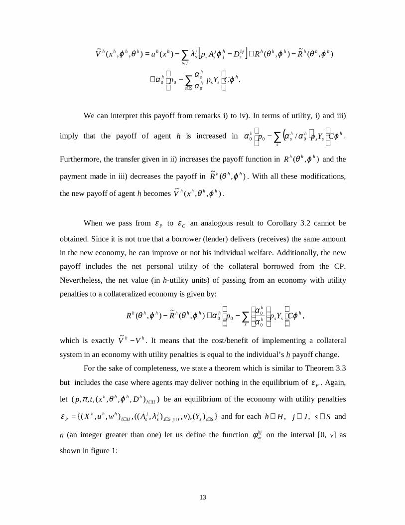
We can interpret this payoff from remarks i) to iv). In terms of utility, i) and iii)

imply that the payoff of agent h is increased in ( ) h

sss

hhs

h CYpp ϕααα

− ∑ 000 / .

Furthermore, the transfer given in ii) increases the payoff function in ),( hhhR ϕθ and the

payment made in iii) decreases the payoff in ),(~ hhhR ϕθ . With all these modifications,

the new payoff of agent h becomes ),,(~ hhhh xV ϕθ .

When we pass from Pε to Cε an analogous result to Corollary 3.2 cannot be

obtained. Since it is not true that a borrower (lender) delivers (receives) the same amount

in the new economy, he can improve or not his individual welfare. Additionally, the new

payoff includes the net personal utility of the collateral borrowed from the CP.

Nevertheless, the net value (in h-utility units) of passing from an economy with utility

penalties to a collateralized economy is given by:

h

sssh

hhhhhhhh CYppRR ϕ

αααϕθϕθ

−+− ∑

0

000),(

~),( ,

which is exactly hh VV −~. It means that the cost/benefit of implementing a collateral

system in an economy with utility penalties is equal to the individual’s h payoff change.

For the sake of completeness, we state a theorem which is similar to Theorem 3.3

but includes the case where agents may deliver nothing in the equilibrium of Pε . Again,

let )),,,(,,,( Hhhhhh Dxtp ∈ϕθπ be an equilibrium of the economy with utility penalties

})(),,),((,),,{( SssJjSsjs

jsHh

hhhP YvAwuX ∈∈∈∈= λε and for each ,Hh∈ ,Jj ∈ Ss∈ and

n (an integer greater than one) let us define the function hjsnφ on the interval [0, v] as

shown in figure 1:

14

The hjsnφ function may be interpreted as a default strategy of the individual h. The net

marginal utility for defaulting by using the strategy hjsnφ is given by:

( )∑ −=js

jhjsn

js

hsnN

,

)()( ϕφλαϕ

We can observe that nN is zero outside of the set Jhj

hj nn )]/1(),/1([ +− ϕϕ . With this

notation we can state our last theorem.

Theorem 3.4 . Let )),,,(,,,( Hhhhhh Dxtp ∈ϕθπ be an equilibrium of the economy with

utility penalties })(),,),((,),,{( SssJjSsjs

jsHh

hhhP YvAwuX ∈∈∈∈= λε . Then for each integer

number 1≥n and each collateral system LJRC ×++∈ , the prices and allocations

)),,(,,( Hhhhhxp ∈ϕθπ is an equilibrium of the economy with collateral requirements

})(,),)((,)~,~

,{(, SssJjjSsj

sHhhh

nh

nC YCAwVX ∈∈∈∈=ε and bounded short sales v, where:

∑∑∑∉∈

−−−−−−+=ss Jj

hs

hj

hjjs

Jj

hj

hj

js

j

hj

hjs

hj

js

js

hs

hs CYCYAtAww ϕϕθϕθϕρθ )()()(~

hhh Cww ϕ+= 00~

and:

( )).(

),(~

)(),,(~

000

,

ϕ

ϕαααϕθϕθαθϕ

n

Ssssh

hshh

jsj

jssj

jss

js

hs

hhn

N

CYppRApAptxuxV

+

−+−−+= ∑∑

∈

hjϕ v

hjsnφ

hjs

hj

jss DAp −ϕ

Figure 1

1/n 1/n

15

We can observe that the payoff function of Theorem 3.4 coincides with that of

Theorem 3.3 except in the set [ ]Jhj

hj nn )/1( ),/1( +− ϕϕ , which decreases as .+∞→n

All the analysis done after Theorem 3.3, with respect to the implementation of a

collateral system in Pε and its individual cost/benefit, is also valid for Theorem 3.4.

5. Concluding Remarks

In the literature of general equilibrium theory with incomplete markets and possibility

of default, the issue concerning the choice of the mechanism to enforce financial

commitments is always discussed. From the theoretical point of view the use of collateral

requirements seems more reasonable. However, the use of utility penalties which

represent either exclusion from the credit markets in future periods or non-economic

punishments has been well received, especially by applied economists.

In this paper we show how these two structures can be compatibilized in order to

explain a specific equilibrium. More precisely, if we consider an equilibrium in a

collateralized economy for loans, it is possible to redefine the payoff function of the

agents to obtain the same equilibrium in this new non-collateralized economy. The payoff

functions are modified in such a way that they embody some sort of punishment if the

agent does not honor at least part of his debt. Conversely, if we have an equilibrium in an

economy with utility penalties and we want to implement a system of collateral

requirements, it is possible to redefine the payoff functions and initial endowments of the

agents to obtain the same equilibrium in the new economy. Lending the collateral and

exchanging the financial earnings of the old system for the corresponding in the new

system we obtain the modified initial wealth. Also, all these modifications imply the

corresponding modification (in utility units) of the payoff function. This is a very natural

way to implement a collateral system in a economy where the default is penalized

directly in the utility function. The hypotheses used for these results are the concavity of

the utility function and the positiveness of the initial endowments.

16

Finally, we offer a discussion on the social welfare of these findings. If we pass from

an economy with collateral requirements to one with utility penalties, the individual’s

welfare is maintained. This is a very interesting result because it affirms that both

mechanisms used to enforce financial commitments are socially equivalent. In

equilibrium the agents achieve the same individual welfare. On the other hand, if we pass

from an economy with utility penalties to one with collateral requirements the individual

payoff may vary. However, the cost/benefit (in utility units) of implementing the new

system equals the variation in the payoff for each individual.

APPENDIX

In most of the proofs we will use the following version of the Karush-Kuhn-Tucker

theorem (see Avriel (1976)). Consider the following maximization problem:

∈=≤

Cx

Mmxg

xf

MP m ,...,1,0)(subject to

)(Maximize

)(

where C is a convex set and RRf n →: and RRg nm →: .

Theorem (*): 1) Suppose that f is a concave function and mg is a convex function

for each m. If Cx ∈* is the solution of (MP) and there exists Cx∈ such that

0)( <<xg (this condition is called Slater’s condition), then there exist Lagrange

multipliers Mmm ,...,1 ;0 =≥λ such that for all Cx∈ we have:

( )∑ −≤−m

mmm xgxgxfxf *)()(*)()( λ

and the complementary conditions: Mmxgmm ,...,1 ;0*)( ==λ

2) If there exist feasible vectors Cx ∈* (i.e 0*)( ≤xg ) and Lagrange multipliers

Mmm ,...,1 ;0 =≥λ such that for all Cx∈ we have:

( )∑ −≤−m

mmm xgxgxfxf *)()(*)()( λ

17

and the complementary conditions: Mmxgmm ,...,1 ;0*)( ==λ , then Cx ∈* is the

solution of (MP).

Proof of Theorem 3.1: The allocation ),,( hhhx ϕθ is optimal for agent h in the

economy Cε , then using theorem (*): there exist 1++∈ Sh Rβ such that for all )1( +×

+∈ SLRx ,

JR+∈ϕθ , ,

( ) ( ){ })()()()())(,())(,( 000000hhhhhh

shhh

sh CxCxpxCxuxCxu ϕϕθθπϕϕβϕϕ −−−++−+≤+−+

( ) .)()()()()( 00∑ ∑ ∑

+−+−−−−+−+s j j

hhss

hjj

js

hjj

js

hsss

hs CxCxYpddxxp ϕϕθθϕϕβ

Then, for any ( ){ }1., ;/Max 000 HhJjCpwpv jjh ∈∈−=≤ πϕ (where JR∈= )1,...,1(1 )

and ],0[ jj

ssj

s ApD ϕ∈ , we can substitute ϕCx +0 by 0x and jss

js

js Aptd = and rewrite

the inequality above as (we will use the h∆ notation for denoting the deviation from the

optimal value):

( ) ( ){ }( )

.

)(

)())(,())(,(

,,

00

000000

∑∑

∑ ∑∑∆−∆+

+−−∆−∆+∆+

∆−∆++−≤+−

js

js

hhs

jsj

hjss

js

hs

s j

hhssj

hjss

js

j

js

hs

hs

hs

hhhhhhs

hhhs

h

DApt

CxxYpAptDxp

CxxpxCxuxxu

βϕβ

ϕθβ

ϕθπϕβϕ

Then we can define ( )∑ −−=js

jsj

jss

js

hss

hh DAptxxuDxV,

0 ))(,(),,(~ ϕβϕ and write

down the inequality above as:

( ) ( ){ }( )∑ ∑∑

+−−∆−∆+∆+

∆−∆++−≤∆

s j

hhssj

hjss

js

j

js

hs

hs

hs

hhhhhhh

CxxYpAptDxp

CxxpV

)(

)(~

00

0000

ϕθβ

ϕθπϕβ

In the economy Cε , the complementary conditions for the agent h maximization

problem are:

18

{ }( ) 0)(

0)()(

0

00000

=

+−−+−

=+−+−

∑∑ hhss

hj

js

hj

js

hs

hss

hs

hhhhh

CxYpddwxp

Cpwxp

ϕθϕβ

πθϕπβ

If we substitute hjs

hjs dD ϕ= and j

jss

js

hj

js Aptd θθ = the complementary conditions

for agent h in the economy Pε will result. Theorem (*) shows the optimality of the

allocation for the new payoff function hV~

in the economy Pε .

The market clear conditions are easily checked.

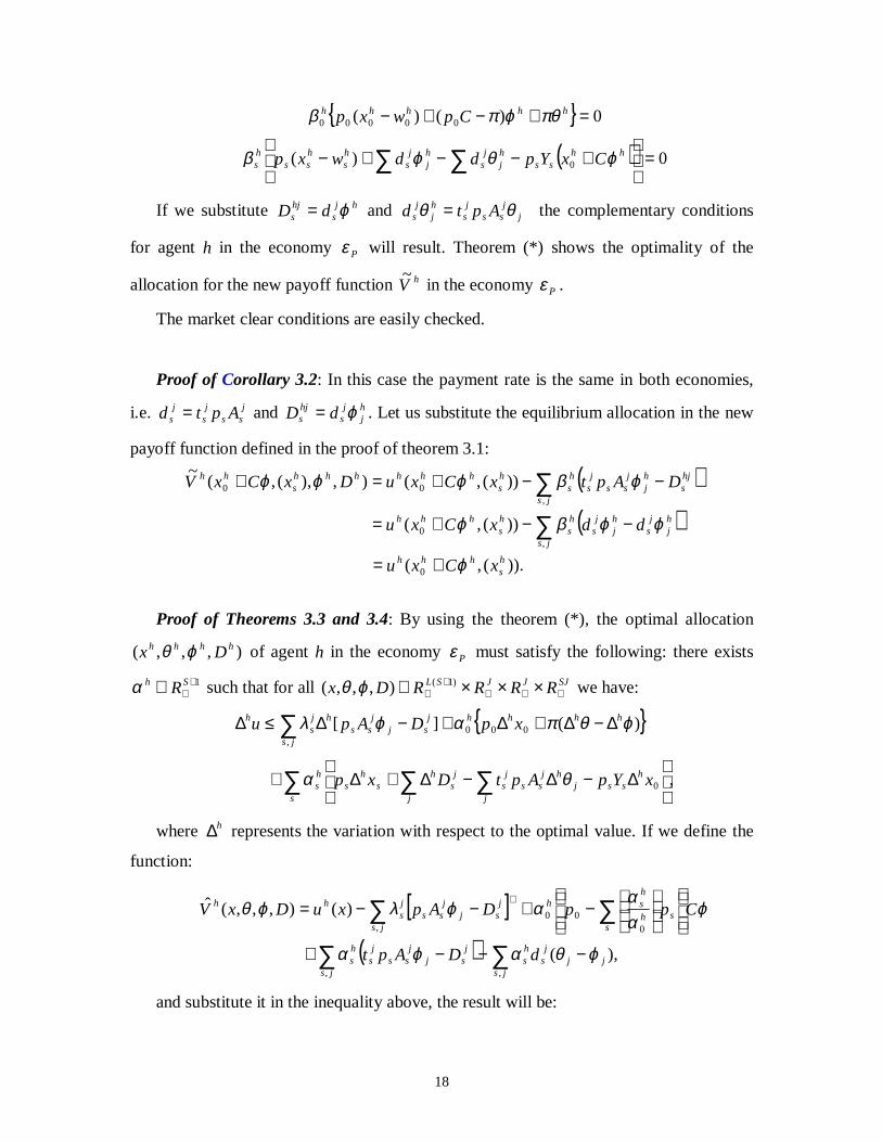
Proof of Corollary 3.2: In this case the payment rate is the same in both economies,

i.e. jss

js

js Aptd = and h

jj

shjs dD ϕ= . Let us substitute the equilibrium allocation in the new

payoff function defined in the proof of theorem 3.1:

( )( )∑

∑−−+=

−−+=+

js

hj

js

hj

js

hs

hs

hhh

js

hjs

hj

jss

js

hs

hs

hhhhhhs

hh

ddxCxu

DAptxCxuDxCxV

,0

,00

))(,(

))(,(),),(,(~

ϕϕβϕ

ϕβϕϕϕ

)).(,( 0hs

hhh xCxu ϕ+=

Proof of Theorems 3.3 and 3.4: By using the theorem (*), the optimal allocation

),,,( hhhh Dx ϕθ of agent h in the economy Pε must satisfy the following: there exists

1++∈ Sh Rα such that for all SJJJSL RRRRDx +++

++ ×××∈ )1(),,,( ϕθ we have:

{ }

,

)(][

0

000,

∑ ∑ ∑

∑

∆−∆−∆+∆+

∆−∆+∆+−∆≤∆

s j j

hssj

hjss

js

js

hs

hs

hs

hhhh

js

jsj

jss

hjs

h

xYpAptDxp

xpDApu

θα

ϕθπαϕλ

where h∆ represents the variation with respect to the optimal value. If we define the

function:

[ ]( ) ,)(

)(),,,(ˆ

,,

, 000

∑∑

∑ ∑−−−+

−+−−=

+

jsjj

js

hs

js

jsj

jss

js

hs

js ssh

hshj

sjj

ssjs

hh

dDApt

CppDApxuDxV

ϕθαϕα

ϕαα

αϕλϕθ

and substitute it in the inequality above, the result will be:

19

∑+≤−s

shs

hhhhhhh LLDxVDxV ααϕθϕθ 00),,,(ˆ),,,(ˆ

where )()( 000 ϕθπϕ hhh CxpL ∆−∆−+∆= and ∑ −∆+∆=j

jjhj

sh

ss dxpL )( θϕ

)( 0 ϕCxYp hss +∆− . To eliminate the variable D from this inequality (because it is not a

decision variable for the individual problem in a collateralized economy) it is sufficient to

consider a D−ϕ path which contains ),( hjs

hj Dϕ in its graph. Using the hj

snφ function

defined before Theorem 3.4, we consider the path )( jhjsnj

jss

js ApD ϕφϕ −= . Substituting

these paths into the function hV̂ we will obtain the following payoff function:

( ).)()(

),(~

)(),,(~

,

000

,

∑

∑∑−+

−+−−+=

∈

jsj

hjsn

js

hs

Ssssh

hshh

jsj

jssj

jss

js

hs

hhn CYppRApAptxuxV

ϕφλα

ϕαααϕθϕθαθϕ

which is exactly the payoff function of Theorem 3.4. To obtain the corresponding payoff

function of Theorem 3.3 we have two cases:

1o.) If 0>= hj

jss

hjs ApD ϕ then 0≡hj

snφ ,

2o.) If ),0( hj

jss

hjs ApD ϕ∈ then j

shs λα = .

This implies that 0≡hjsnφ . Therefore if 0>>hD then the payoff function of Theorem

3.3 results.

The complementary conditions are easily checked. So we have the optimality of

),,( hhhx ϕθ on the budget constraint of individual h with payoff function hnV

~ in the

economy with collateral system C.

The proof of the market clear conditions for the first period is straightforward. For the

second period we need to define the set }/{ jssj

sss CYpApJjJ ≤∈= (the set of all

assets whose promises are honored in state s). Then, the initial endowment of agent h in

state s can be written as:

∑∑∑∉∈

−−−−−−+=ss Jj

hs

hj

hjjs

Jj

hj

hj

js

j

hj

hjs

hj

js

js

hs

hs CYCYAtAww ϕϕθϕθϕρθ )()()(~ .

20

Then, from the market clear conditions of the second period of the economy Pε and

the following identity: ∑

∑=

h

hj

h

hj

hjs

jst ϕ

ϕρ, we obtain the market clear conditions of the

second period for the economy Cε .

References

Araujo A., Páscoa M. and Torres-Martinez J., “Collateral Avoids Ponzi

Schemes in Imcomplete Markets”, Econometrica, Vol. 70, No. 4, (2002), pp. 1613-1638.

Avriel M., Nonlinear programming - Analysis and Methods .

Englewood Cliff, N. J.: Prentice-Hall, Inc. (1976).

Dubey P., Geanakoplos J. and Shubik M., “Default and punishment in

general equilibrium”, Econometrica, Vol. 73 – 1, (2005), 1 - 37.

Geanakoplos J. and Zame W., “Collateral and the Enforcement of

Intertemporal Contracts”, Yale University Working Paper (2002).

Goodhart Ch., Sunirand P. and Tsomocos D., “A Model to Analyse

Financial Fragility”, Oxford Financial Research Centre Working Paper No. 2003fe13.

(2003a).

Goodhart Ch., Sunirand P. and Tsomocos D., “A Model to Analyse

Financial Fragility: Applications”, Mimeo Bank of England. (2003b).

Kubler, F., Schmedders, K., “Stationary Equilibria in Asset-Pricing Models

with Incomplete Markets and Collateral” , Econometrica, 71(6), (2003), pp.1767-1793.

21

Orrillo, J., “Making Promises in Infinite-Horizon Economies with Default”,

Catholic University of Brasilia Working Paper, (2002).

Zame W., “Efficiency and the Role of Default when Security Markets are

Incomplete”, American Economic Review 83 (1993), 1142-1164.