Collateral and relationship lending in loan pricing ... · Collateral and relationship lending in...
15
Collateral and relationship lending in loan pricing: Evidence from UK SMEs ANA PAULA MATIAS GAMA 1 & FÁBIO DIAS DUARTE 2 Management and Economics Department NECE – Research Unit in Business Sciences University of Beira Interior, Estrada do Sineiro, 6200-209 Covilhã PORTUGAL 1 [email protected]; 2 [email protected] Abstract: This study investigates how the use of collateral affects incentives for borrowers and lenders and the resulting loan pricing relationship. With data from the UK Survey of Small and Medium-Sized Enterprises 2008, a simultaneous equation approach reveals that high quality borrowers choose contracts with more collateral and lower interest rates, which suggests that collateral acts as an incentive in credit markets. By distinguishing business from personal collateral, the present study also reveals that personal collateral seems more effective as a sorting device, in line with screening models. Regarding the nature of the borrower–lender relationship, a substitution effect arises between relationship length and collateral requirements, but a primary bank uses an explicit loan interest rate as a loss leader to secure long-term rents on relationship business, suggesting the possibility of intertemporal shifting rents. Keywords: credit rationing, loan pricing, collateral, relationship lending, small and medium-sized enterprises 1. Introduction Microeconomic theories of banking and financial intermediation [30] explain the widespread use of collateral by noting that collateral reduces credit rationing for under asymmetric information. Theoretical credit rationing occurs in equilibrium if the demand for loans exceeds the supply at the prevailing interest rate [50]. Because banks’ expected return increases nonmonotonously with interest rate increases, banks prefer rationing credit to opaque firms (e.g., small and young firms) rather than increasing interest rates [50]. In such situations, collateral provides important means for the bank to mitigate informational asymmetries and solve the credit-rationing problem. Pledging collateral to secure loans is a common feature of credit acquisition. Cressy and Toivanen [26] report that 85% of UK loans require collateral, as do 70% of US loans [6]. Credit market research explains the use of collateral as a consequence of adverse selection [8] [9] [10] [19], or moral hazard [15] in transactions between borrowers and lenders. The nature of the borrower–lender relationship [43] [46], the level of competition in the credit market [8], and the net cost (benefits) of a through screening of borrowers also might explain the simultaneous existence of secured and unsecured loans [40] (for an extensive research survey, see Coco [22]). However, theoretical and empirical studies on the use of collateral to reduce informational asymmetry do not provide consistent results. The seemingly contradictory results may reflect the research methods, which fail to address simultaneity in debt terms; that is, lenders do not determine the interest rate separately from other loan terms. An analytic framework for price-setting behavior by banks and information availability about small and medium-sized enterprises (SMEs) thus remains underdeveloped [4]. To extend understanding of the pricing behavior of banks, this study investigates how the use of collateral affects incentives for borrowers and lenders and their relationship. First, the present study examines if good borrowers offer collateral to signal their low risk type and obtain a loan contract with a lower interest rate (adverse selection effect) or if riskier borrowers instead must provide collateral (moral hazard effect). Second, this study investigates how borrower–lender relationships affect debt term contracts. Existing literature (e.g., [17], [37]) establishes the endogenous determination of collateral requirements; therefore, the present study examines the main loan contracts terms (i.e., interest rate and collateral requirements) using simultaneous equation modeling. In the context of WSEAS TRANSACTIONS on BUSINESS and ECONOMICS Ana Paula Matias Gama, Fábio Dias Duarte E-ISSN: 2224-2899 21 Volume 12, 2015
Transcript of Collateral and relationship lending in loan pricing ... · Collateral and relationship lending in...

Collateral and relationship lending in loan pricing: Evidence from
UK SMEs
ANA PAULA MATIAS GAMA
1 & FÁBIO DIAS DUARTE
2
Management and Economics Department
NECE – Research Unit in Business Sciences
University of Beira Interior,
Estrada do Sineiro, 6200-209 Covilhã
PORTUGAL [email protected];
Abstract: This study investigates how the use of collateral affects incentives for borrowers and lenders and the
resulting loan pricing relationship. With data from the UK Survey of Small and Medium-Sized Enterprises
2008, a simultaneous equation approach reveals that high quality borrowers choose contracts with more
collateral and lower interest rates, which suggests that collateral acts as an incentive in credit markets. By
distinguishing business from personal collateral, the present study also reveals that personal collateral seems
more effective as a sorting device, in line with screening models. Regarding the nature of the borrower–lender
relationship, a substitution effect arises between relationship length and collateral requirements, but a primary
bank uses an explicit loan interest rate as a loss leader to secure long-term rents on relationship business,
suggesting the possibility of intertemporal shifting rents.
Keywords: credit rationing, loan pricing, collateral, relationship lending, small and medium-sized enterprises
1. Introduction Microeconomic theories of banking and financial
intermediation [30] explain the widespread use of
collateral by noting that collateral reduces credit
rationing for under asymmetric information.
Theoretical credit rationing occurs in equilibrium if
the demand for loans exceeds the supply at the
prevailing interest rate [50]. Because banks’
expected return increases nonmonotonously with
interest rate increases, banks prefer rationing credit
to opaque firms (e.g., small and young firms) rather
than increasing interest rates [50]. In such situations,
collateral provides important means for the bank to
mitigate informational asymmetries and solve the
credit-rationing problem.
Pledging collateral to secure loans is a common
feature of credit acquisition. Cressy and Toivanen
[26] report that 85% of UK loans require collateral,
as do 70% of US loans [6]. Credit market research
explains the use of collateral as a consequence of
adverse selection [8] [9] [10] [19], or moral hazard
[15] in transactions between borrowers and lenders.
The nature of the borrower–lender relationship [43]
[46], the level of competition in the credit market
[8], and the net cost (benefits) of a through
screening of borrowers also might explain the
simultaneous existence of secured and unsecured
loans [40] (for an extensive research survey, see
Coco [22]). However, theoretical and empirical
studies on the use of collateral to reduce
informational asymmetry do not provide consistent
results. The seemingly contradictory results may
reflect the research methods, which fail to address
simultaneity in debt terms; that is, lenders do not
determine the interest rate separately from other
loan terms. An analytic framework for price-setting
behavior by banks and information availability
about small and medium-sized enterprises (SMEs)
thus remains underdeveloped [4].
To extend understanding of the pricing behavior
of banks, this study investigates how the use of
collateral affects incentives for borrowers and
lenders and their relationship. First, the present
study examines if good borrowers offer collateral to
signal their low risk type and obtain a loan contract
with a lower interest rate (adverse selection effect)
or if riskier borrowers instead must provide
collateral (moral hazard effect). Second, this study
investigates how borrower–lender relationships
affect debt term contracts. Existing literature (e.g.,
[17], [37]) establishes the endogenous determination
of collateral requirements; therefore, the present
study examines the main loan contracts terms (i.e.,
interest rate and collateral requirements) using
simultaneous equation modeling. In the context of
WSEAS TRANSACTIONS on BUSINESS and ECONOMICS Ana Paula Matias Gama, Fábio Dias Duarte
E-ISSN: 2224-2899 21 Volume 12, 2015

SMEs, the owner’s personal wealth frequently
facilitates access bank loans, so this study also
distinguishes business collateral from personal
collateral.
2. Relevance The consolidation of the banking industry and the
introduction of the Basel II Capital Accord requires
information-opaque firms to rely heavily on
collateral [34]. Consolidation increases the use of
transaction-lending technologies [5], which depend
on particular information, such as financial
statements, accounts receivable, inventory, and
credit scores. Only SMEs that can provide collateral
to secure loan repayment generally receive bank
credit [5]. The Basel II Capital Accord should
increase the importance of collateral further. The
Basel I Capital Accord treated all corporate lending
alike; Basel II prescribes that banks that engage in
higher risk lending must hold more capital to
safeguard their solvency and overall economic
stability [3]. Thus banks prefer collateralized loans
to reduce loan portfolio risk [3].
Studies of loan collateralization in various
countries often rely on banks’ credit files (e.g., [1]
[2] [6] [17] [26] [27] [32] [36] [38]). This study
adopts a data set based on the UK Survey of Small
and Medium-Sized Enterprises (UKSMEF),
conducted by the Center for Small and Medium-
Sized Enterprises (CSME) at Warwick Business
School. In turn, by examining interactions among
collateralization, interest rate premium, and
relationship lending techniques in debt term
contracts with SMEs, this study contributes to extant
literature in several ways. First, with a simultaneous
equation modeling approach, this study examines
the simultaneous impact of the borrower–lender
relationship on the explicit interest rate and thus on
collateral. Accounting for interdependences between
contractual debt term conditions may clarify
previously ambiguous results. Second, by
distinguishing business from personal collateral, this
study identifies personal collateral as more effective
as a sorting device, in line with screening models.
High quality firms prefer to pledge personal
collateral, because with this strategy, borrowers can
avoid more restrictive usage of business collateral.
For the lender, personal collateral is more effective
in limiting the borrower’s risk incentives, because
the owner likely will feel personal consequences of
any ex post managerial shirking or risk taking.
Bonding by personal collateral also avoids more
costly monitoring of business collateral or covenants
[33] [45].
The next section presents an overview of the role
of collateral in mitigating informational
asymmetries, which helps solve credit rationing, and
develops empirical hypotheses. After a description
of the data, variables, and empirical method, this
article presents and discusses the results and finally
concludes with some key insights.
3. Literature review and hypotheses 3.1 Credit rationing: an overview Bank loans are the most widely used form of SME
financing [29] [53], though exchange relationships
often suffer from market imperfections, such as
information asymmetries [24] [25] [50] [54] that
occur when lenders have little reliable information
about the applicants’ default risk [8]. Because SMEs
rarely are listed firms, they have trouble signaling
their qualities to financial institutions [25] [54].
Such firms also may be unwilling to release
information, which is time consuming and costly.
This dilemma creates the so-called opacity problem
[5].
The information asymmetry between banks and
SMEs can be severe enough to induce credit
rationing, which occurs when demand for loans
exceeds supply at the prevailing interest rate [50].
Rationing implies that borrowers either do not
receive the full credit they request (type I rationing)
or receive no credit at all (type II rationing). Excess
demand for bank funds should lead banks to raise
loan prices (interest rates), but this tactic is rare in
the normal course of bank lending, because banks
have no real incentive to raise interest rates when
demand exceeds supply. As Steijvers and
Voordeckers [49] recognize, the bank-optimal
interest rate is the equilibrium interest rate, because
above this rate, the bank’s expected return increases
at a rate slower than the interest rate and even
decreases beyond a certain interest rate. Some
borrowers that do not receive bank credit would pay
a higher interest rate, and a bank that charges this
higher interest rate attracts riskier borrowers
(adverse selection effect). The adverse selection
effect means that the lending bank ex ante cannot
detect borrower quality, which gives the firm an
unfair advantage. If banks raise the interest rate,
borrowers prefer even more risky projects, which
reduces bank returns further, through the moral
hazard effect [49]. Thus even in equilibrium,
demand will not equal the supply, and banks prefer
to ration credit [50]. Yet theoretical models of the
effects of increased loan prices on a lender’s
portfolio (e.g., [8] [9] [10] [11]) often assume credit
WSEAS TRANSACTIONS on BUSINESS and ECONOMICS Ana Paula Matias Gama, Fábio Dias Duarte
E-ISSN: 2224-2899 22 Volume 12, 2015

term contracts that include only the terms of the
interest rate or collateral, without considering
possible interdependences (cf.[22]).
3.2 Joint collateral and interest rate
considerations in loan pricing According to Jensen and Meckling [35], signaling
and monitoring can address agency conflict. A
solution to the adverse selection problem relies on
incentive compatibility contracts with signals about
the quality of different agents. Firms that want to
signal creditworthiness thus use collateral widely,
instead of more costly monitoring tools [51]. To
avoid incentive effects though, covenants must be
very detailed and cover all aspects of the firm,
which is almost impossible. If collateral value is
stable or more objectively ascertainable than the
distribution of returns, an entrepreneur could trade
profitably for better interest rates [19].
A bank that possesses two informative
instruments may want to use both jointly, as
predicted in screening models (e.g. [8] [9] [10]
[11]). Banks simultaneously consider collateral
requirements and interest rates to screen investors’
riskiness, which supports the use of different
contract terms as a self-selection mechanism to
separate borrowers with different risk levels.
Collateral signals high credit quality in adverse
selection situations in which borrowers know their
credit quality but lenders do not [19]; borrowers
with a higher probability of default instead choose a
contract with a higher interest rate and lower
collateral.
H1: High quality (low quality) borrowers choose a
contract with more (less) collateral and a lower
(higher) interest rate.
If lenders can observe the borrower’s credit
quality ex ante [15] but information asymmetry
arises after the loan, collateral mitigates moral
hazard by limiting the behavior of the borrower
[12]. Collateral prevents a firm from switching from
a lower to a higher risk project after receiving the
loan (i.e., asset substitution [35]) or exerting less
effort [15]. Accordingly, lenders ask riskier
borrowers to put up more collateral, whereas low
risk borrowers obtain loans without having to
pledge collateral [6].
H2: High risk firms pledge more collateral than
low-risk borrowers.
If an inverse relation marks collateral and
interest rates, as a function of the borrower’s private
information (H1), collateral acts as a mechanism to
show the borrower’s risk preferences ex ante. To
measure private information known only by the
borrower, this study uses credit quality as a dummy
variable, which reflects borrowers’ perception of
their financial situation (see Section 4.2). The data
set lacks information about to ex post event defaults,
so risk measures reflect firm size [28]. Larger firms
tend to be more diversified and have an historical
performance track record [18], so this study expects
that firm size relates negatively to risk and thus loan
collateralization.
A firm that receives more debt attains higher
leverage and increases the risk of non-payment [21],
leading banks to ask for more collateral protection
[27]. Because pledging collateral creates costs that
borrowers can recover only with large loans and
economies of scale, the likelihood of pledging
collateral is higher for larger loan sizes [54]. Long-
term debt also gives the borrower more
opportunities to alter the project [35], but collateral
helps the lender ascertain a certain future value.
Even if the company loses its value in the longer
term, the collateral retains value [39]. This asset
cannot belong to another creditor, so by asking for
collateral, the bank ensures the priority of its loan
and creates a barrier to other creditors. Thus, loan
size and loan maturity period should increase the
amount of secured debt.
H3: Loan size relates positively to collateral
requirements and negatively to interest rates.
H4: Loan maturity period relates positively to with
collateral requirements and negatively to interest
rates.
Business and personal collateral could have
differential signaling value for agency problems.
Business collateral does not expose owners
themselves to risk and thus should benefit the firm’s
owners. John et al. [37] find a positive relation of
the use of business collateral, firm risk, and interest
rate; for SMEs though, the owner frequently uses
personal wealth to access bank loans [1], so
personal collateral may be a better signal of quality.
The owner of a lower quality firm cannot afford to
imitate a high quality firm [17]; in this sense,
personal collateral effectively limits the borrower’s
risk preferences by enhancing the likelihood that the
owner suffers the consequences of any ex post
managerial shirking or risk-taking activities [39].
Personal collateral also can substitute for equity
WSEAS TRANSACTIONS on BUSINESS and ECONOMICS Ana Paula Matias Gama, Fábio Dias Duarte
E-ISSN: 2224-2899 23 Volume 12, 2015

investments, and in the case of default, the sale of
personal assets could help repay the loan. Therefore
this study expects that the economic impact of a
requirement to pledge personal collateral should be
greater than that of pledging business collateral.
3.3 Impact of borrower–lender relationship
strength on loan pricing Reliable information on SMEs is rare and costly, so
relationship lending is an appropriate lending
technique [27] [54]. Good lending relationships
facilitate information exchange, because lenders
invest to obtain information from clients, and
borrowers have a motivation to disclose [14]. Over
time, an entrepreneur can establish a reputation by
demonstrating a preference for low-risk projects and
experiencing few repayment difficulties [28], which
also grants the bank a more complete picture of the
firm’s financial health [13].
Measures of relationship strength often
focus on duration [41]. A long-term relationship
allows a lender to gather more private information
about the borrower, such as capacities and character,
that is difficult to observe or accumulate [5].
Information generated through repeated transactions
and over time also helps reduce the fixed costs of
screening and monitoring [14], which can minimize
the free-rider problem because the bank internalizes
the benefits of investments. The relation between
borrower and lender should facilitate ex ante
screening and ex post monitoring and mitigate
informational opaqueness.
H5: Relationship length relates negatively to
collateral requirements.
Scope is another dimension of relationship
strength [42], defined as the quantity of products or
services the borrower shares with the bank.
Concentrated scope increases sources of information
for the bank and dilutes information collection costs
to enhance economies of scale [28]. The intense
interaction and exchange of information reduces
information asymmetry, reinforces mutual trust, and
minimizes banks’ lending risk, which should lead to
lower collateral requirements.
H6: The scope of the borrower–lender relationship
relates negatively to collateral requirements.
However, a solid relationship may become
detrimental to the borrower if a primary lender
exerts an information monopoly and charges high
interest rates or requires more collateral (i.e., hold-
up problem) [46]. Initiating a second lending
relationship would be costly for the borrower, which
hopes to avoid switching costs and thus gets locked
in [14]. In line with Petersen and Rajan’s [42]
bargaining hypothesis, this study predicts:
H7: Relationship length relates positively to interest
rate premiums.
Because collateral reduces a bank’s risk
exposure, the bank might grow less careful or
engage in risky lending (“lazy bank” argument)
[40]. Borrowers with lasting relationships with a
risky lender then must pay for the losses accrued
through an inefficient allocation of resources [38].
4. Data, method, and variables 4.1. Data The UKSMEF by the CSME started in 2004 with
funding from a consortium of public and private
organizations, led by the Bank of England. The
2008 survey included 2500 SMEs (from the UK
population of 4.4 million), defined as firms with
fewer than 250 employees in the private sector.1 The
sample structure supported analyses by size, sector,
and government standard regions. These data offer
three key advantages. First, the UKSMEF provides
information about whether each borrower pledges
business or personal collateral to a primary lender,
as well as the interest rate premium paid. Second,
the survey features various detailed questions about
the number of years the borrower and its primary
bank conducted transactions and the types of
financial services the relationship involves. This
information supports analyses of how business and
personal collateral and the interest rate premium
relate to the borrower–lender relationship. Third, the
survey includes questions about firms’ perceptions
of risk levels and the history of past defaults of the
firm or owner.
However, data related to the financial statements
are scarce. Questions refer to the transactions
between a firm and a primary bank, not individual
loan contracts. If a firm has multiple loans with a
single bank, data about the usage rates of personal
and business collateral and the interest rate premium
charged may be biased. The survey also does not
identify the lender, so this study cannot match firm-
level data with financial variables or construct a
Herfindahl index. In turn, no control for lender
1 See UK Data Archive Study number 6314, United
Kingdom Survey of Small and Medium-Sized Enterprises
Finances, 2008.
WSEAS TRANSACTIONS on BUSINESS and ECONOMICS Ana Paula Matias Gama, Fábio Dias Duarte
E-ISSN: 2224-2899 24 Volume 12, 2015
characteristics appears. Finally, the UKSMEF
survey deals only with surviving firms, though some
firms previously defaulted. To analyze price-setting
behavior by banks, the chosen data set includes only
firms that request bank credit. The final sample for
empirical analysis features 326 SMEs.
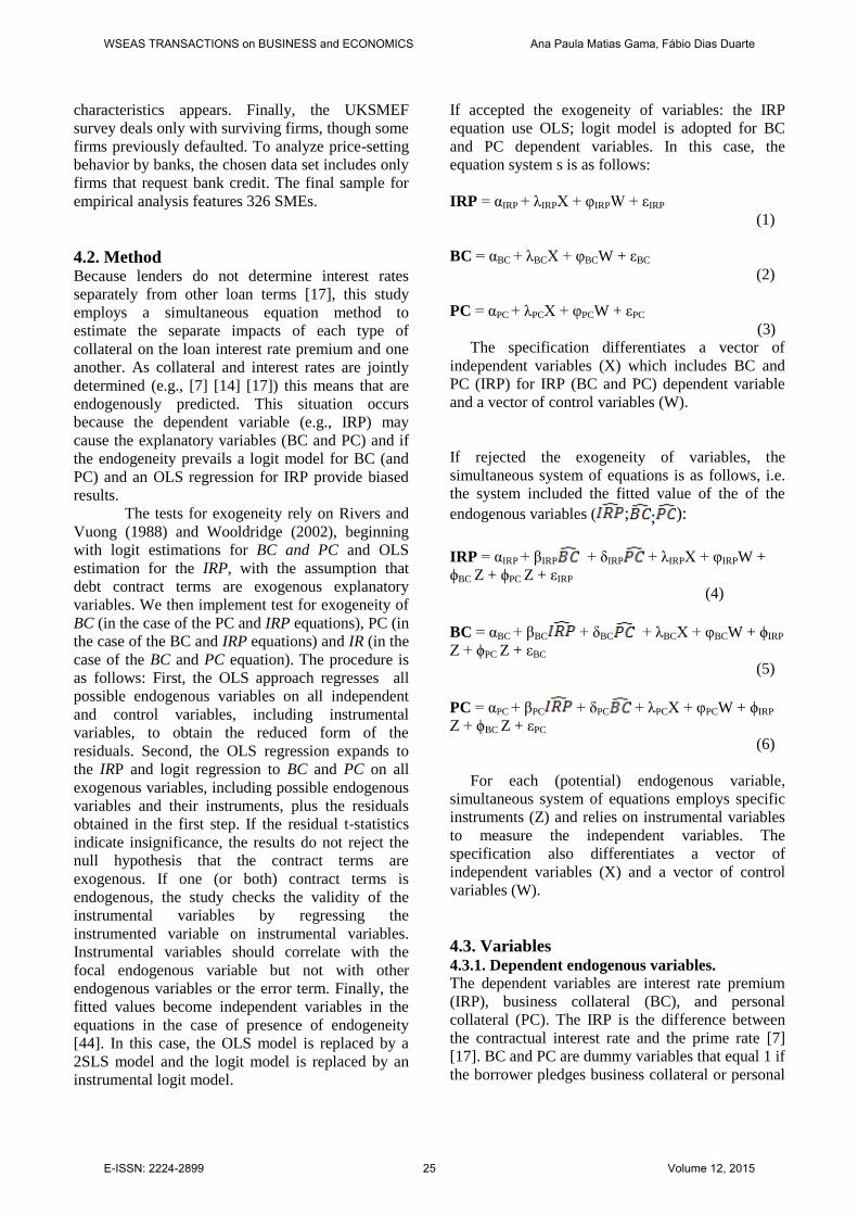
4.2. Method Because lenders do not determine interest rates
separately from other loan terms [17], this study
employs a simultaneous equation method to
estimate the separate impacts of each type of
collateral on the loan interest rate premium and one
another. As collateral and interest rates are jointly
determined (e.g., [7] [14] [17]) this means that are
endogenously predicted. This situation occurs
because the dependent variable (e.g., IRP) may
cause the explanatory variables (BC and PC) and if
the endogeneity prevails a logit model for BC (and
PC) and an OLS regression for IRP provide biased
results.
The tests for exogeneity rely on Rivers and
Vuong (1988) and Wooldridge (2002), beginning
with logit estimations for BC and PC and OLS
estimation for the IRP, with the assumption that
debt contract terms are exogenous explanatory
variables. We then implement test for exogeneity of
BC (in the case of the PC and IRP equations), PC (in
the case of the BC and IRP equations) and IR (in the
case of the BC and PC equation). The procedure is
as follows: First, the OLS approach regresses all
possible endogenous variables on all independent
and control variables, including instrumental
variables, to obtain the reduced form of the
residuals. Second, the OLS regression expands to
the IRP and logit regression to BC and PC on all
exogenous variables, including possible endogenous
variables and their instruments, plus the residuals
obtained in the first step. If the residual t-statistics
indicate insignificance, the results do not reject the
null hypothesis that the contract terms are
exogenous. If one (or both) contract terms is
endogenous, the study checks the validity of the
instrumental variables by regressing the
instrumented variable on instrumental variables.
Instrumental variables should correlate with the
focal endogenous variable but not with other
endogenous variables or the error term. Finally, the
fitted values become independent variables in the
equations in the case of presence of endogeneity
[44]. In this case, the OLS model is replaced by a
2SLS model and the logit model is replaced by an
instrumental logit model.
If accepted the exogeneity of variables: the IRP
equation use OLS; logit model is adopted for BC
and PC dependent variables. In this case, the
equation system s is as follows:
IRP = αIRP + λIRPX + φIRPW + εIRP
(1)
BC = αBC + λBCX + φBCW + εBC
(2)
PC = αPC + λPCX + φPCW + εPC
(3)
The specification differentiates a vector of
independent variables (X) which includes BC and
PC (IRP) for IRP (BC and PC) dependent variable
and a vector of control variables (W).
If rejected the exogeneity of variables, the
simultaneous system of equations is as follows, i.e.
the system included the fitted value of the of the
endogenous variables ( ; ; ):
IRP = αIRP + βIRP + δIRP + λIRPX + φIRPW +
ϕBC Z + ϕPC Z + εIRP
(4)
BC = αBC + βBC + δBC + λBCX + φBCW + ϕIRP
Z + ϕPC Z + εBC
(5)
PC = αPC + βPC + δPC + λPCX + φPCW + ϕIRP
Z + ϕBC Z + εPC
(6)
For each (potential) endogenous variable,
simultaneous system of equations employs specific
instruments (Z) and relies on instrumental variables
to measure the independent variables. The
specification also differentiates a vector of
independent variables (X) and a vector of control
variables (W).
4.3. Variables 4.3.1. Dependent endogenous variables.
The dependent variables are interest rate premium
(IRP), business collateral (BC), and personal
collateral (PC). The IRP is the difference between
the contractual interest rate and the prime rate [7]
[17]. BC and PC are dummy variables that equal 1 if
the borrower pledges business collateral or personal
WSEAS TRANSACTIONS on BUSINESS and ECONOMICS Ana Paula Matias Gama, Fábio Dias Duarte
E-ISSN: 2224-2899 25 Volume 12, 2015

collateral, respectively. Table 1 contains all the
variable definitions.
4.3.2. Independent and control variables.
The independent variables reflect firm, loan, and
borrower–lender relationship characteristics. Firm
variables include credit quality (H1) and firm size
(H2). The UKSMEF database defines a binary
dummy variable as equal to 1 if the firm shows little
financial distress, which is somewhat subjective
because each respondent defines its own final
situation. This study uses “credit quality” as a proxy
for private information, which the lender does not
have or knows only imperfectly. Literature suggests
that firm size is one of the most relevant input in the
credit risk assessment (e.g., [48]). Hence, this study
includes “firm size”, that is the natural logarithm of
the firm’s total assets, to predict the loan price
terms.
Loan characteristics include “loan size” (H3)
(i.e., natural logarithm of loan size, measured in
pounds), “loan maturity” (H4) (i.e., natural
logarithm of loan maturity in years), a binary
variable (“fixed rate”) that controls if the loan has a
fixed rate [17], and the fitted values for collateral
requirements and interest rate premium, obtained
from an instrumental variable technique.
For the borrower–lender variables, this study
includes relationship “length” (H5, H7) with the
main bank (i.e., natural logarithm of the number of
years the firm has dealt with its main bank) and
variable “scope" (H6), or the number of financial
products the borrower has purchased from the
primary bank [20]. The UKSMEF asks firms to list
all products/services, other than loans, they have
purchased. The measure is the number of products
for each firm, divided by the total products offered
by the primary bank.
Finally, this study controls for industry and
organizational form considering that there are
differences in the risk exposure across different
activity sectors [48] and organizational legal status
[7]. Nine dummy variables account for industry
differences. To capture possible differences in
collateral requirements, this study features four
dummy variables for firm organization: S-
corporation, C-corporation, limited liability
company, and limited liability partnership.
4.3.3. Instrumental variables
The instrumental variable in the interest rate
premium equation is firm delinquency, a dummy
equal to 1 if the firm has previously defaulted and 0
otherwise. Bank uses past information to classify
current customer as good or bad customer [23].
Hence, the likelihood that a lender imposes a higher
interest rate should relate positively to whether the
firm has defaulted previously [31]
For the bank, collecting information about small
firms is costly [45], so banks rely on the use of
collateral requirements, especially fixed assets with
Table 1: Variable definitions
Variable Definition
Dependent variables
IRP Difference between the contractual interest rate and the prime rate
BC Equals 1 if the firm is required to post business collateral (0,1)
PC Equals 1 if the owner is required to post personal collateral/guarantees (0,1)
Independent variables
Credit quality Equals 1 if the firm show a low level of financial distress (0,1)
Firm size Natural logarithm of firm’s total assets
Loan size Natural logarithm of the loan size measured in pounds
Loan maturity Natural logarithm of the loan maturity in years
Fixed rate Equals 1 if the loan has a fixed rate (0,1)
Length Natural logarithm of the relationship length in years with the main bank
Scope Number of financial products the firms has purchased from the main bank
Control variables
Industry Equals 1 it the firms belongs to industry x (x ϵ [1,9] to distinguish between 9 industries) (0,1)
S-corp. Equals 1 it he firm is organized as a S-corporation (0,1)
C-corp. Equals 1 it he firm is organized as a C-corporation (0,1)
LLC Equals 1 it he firm is organized as a limited liability company (0,1)
LLP Equals 1 it he firm is organized as a limited liability partnership (0,1)
Instrumental variables
Firm delinquency Equals 1 if the firms has previously defaulted (0,1)
Fixed assets Equals 1 if the loan must be supported by a compensating balance sheet assets (0,1)
CEO age Natural logarithm of the age of the CEO in years
WSEAS TRANSACTIONS on BUSINESS and ECONOMICS Ana Paula Matias Gama, Fábio Dias Duarte
E-ISSN: 2224-2899 26 Volume 12, 2015

relatively stable value, that also signal the bank’s
priority among creditors [14]. Securing credit limits
a firm’s ability to obtain future loans from another
lender and mitigates the possibility of selling
business assets to invest in new projects [47] or
perks [37]. Thus, the business collateral equation
uses the fixed assets variable as an instrumental
variable equal to 1 if the loan requires support from
a compensating balance sheet fixed asset, and 0
otherwise. However, Mann [39] argues that personal
collateral is more effective in limiting a borrower’s
risk incentives by increasing the likelihood that the
owner suffers the consequences of ex post
managerial shirking. For the personal collateral
equation, this study uses the natural logarithm of the
age of the CEO/owner as an instrumental variable.
Younger borrowers provide scant information in
commercial and financial records; over time,
information accumulates [28] [23]. The study
follows Bolton [16] to assume that small businesses
feature the same individual and/or family
ownership.
The tests for exogeneity rely on the method of
Rivers and Vuong [44] and Wooldridge [52],
beginning with OLS estimations for the IRP
variable and logit estimations for BC and PC, with
the assumption that debt contract terms are
exogenous explanatory variables. First, the OLS
approach regresses all possible endogenous
variables on all independent and control variables,
including instrumental variables, to obtain the
reduced form of the residuals. Second, the OLS
regression expands to the IRP and logit regression to
BC and PC on all exogenous variables, including
possible endogenous variables and their instruments,
plus the residuals obtained in the first step. If the
residual t-statistics indicate insignificance, the
results do not reject the null hypothesis that the
contract terms are exogenous. If one (or both)
contract terms is endogenous, the study checks the
validity of the instrumental variables by regressing
the instrumented variable on instrumental variables.
Third, the fitted values become independent
variables in the IRP rate, BC, and PC equations.
5. Results 5.1. Descriptive analysis
Table 2. OLS estimation for interest rate premium/logistic estimation for business and personal collateral and exogeneity tests
Panel A: OLS and logistic estimations
IRP (OLS) BC (LOGIT) PC (LOGIT)
Coef.
(1)
T-stat. Coef.
(2)
Wald-test. Coef.
(3)
Wald-test.
IRP -0.006 (0.058) 0.012 0.031 (0.063) 0.244
BC 0.024 (0.312) 0.077 -1.778 (0.406) 19.189***
PC 0.155 (0.344) 0.451 -1.734 (0.419) 17.108***
Credit quality -0.224 (0.278) -0.804 0.571 (0.281) 4.135** 0.144 (0.302) 0.226
Firm size -0.150 (0.084) -1.794* 0.254 (0.087) 8.566*** -0.150 (0.091) 2.733*
Loan size -0.358 (0.121) -2.949*** 0.299 (0.139) 4.653** 0.323 (0.151) 4.553**
Loan maturity 0.074 (0.210) 0.354 0.699 (0.229) 9.310*** 0.237 (0.233) 1.030
Fixed rate 2.493 (0.284) 8.786*** -0.384 (0.328) 1.372 -0.636 (0.362) 3.085*
Length 0.247 (0.139) 1.781* 0.131 (0.145) 0.817 -0.127 (0.159) 0.634
Scope 0.146 (0.774) 0.189 -0.631 (0.824) 0.586 -0.079 (0.862) 0.008
Firm
delinquency
0.864 (0.333) 2.595***
Fixed assets 0.525 (0.278) 3.559*
CEO age 1.318 (0.737) 3.198*
Constant 8.871 (1.461) 6.073*** -9.431 (1.865) 25.560*** -8.306 (3.222) 6.644***
Obs. 326 326 326
R-squared/Log-
Likelihood
0.322 329.615 288.709
Panel B: Exogeneity Tests
resid_IRP 1.51 (1.422) 1.127 -1.986 (0.907) 4.791**
resid_BC 0.745 (1.554) 0.479 39.112 (6.847) 32.633***
resid_PC -13.320 (2.788) -4.778*** 329.102 (124.817) 6.952***
Standard errors are reported in parentheses. This study controls for industry (nine dummy variables) and organizational form (four dummy
variables), but the results do not appear in this table. *** Statistically significant at 1% level.** Statistically significant at 5% level. *
Statistically significant at 10% level
WSEAS TRANSACTIONS on BUSINESS and ECONOMICS Ana Paula Matias Gama, Fábio Dias Duarte
E-ISSN: 2224-2899 27 Volume 12, 2015

Appendix contains the focal descriptive statistics
and correlations, though not for the control
variables. Whereas 36% of firms pledged BC, 21%
pledged PC, and the mean IRP is 4.35% (median =
5%). At the mean, firms have 1,519,540 in total
assets, and 58% of firms self-identify as low risk
borrowers. Average relationship length with the
main bank is 14.5 years, and firms purchase more
than 50% of their financial services (scope) from
this main bank (mean = 55%). Regarding loan
characteristics, the mean value of loan size is
546,074 pounds, with a maturity of 9.6 years, and
40% of firms negotiate fixed rates.
The correlation values for the independent
variables are less than 0.5, so multicollinearity was
not a problem [52]. The Spearman correlations for
the coefficient estimation provide a non-parametric
technique based on ranks rather than the value of the
variables.
5.2. Empirical results Panel A of Table 2 contains the benchmark
estimation (i.e., OLS for IRP, logistic estimation for
BC and PC) when all the loan contract terms are
exogenous variables. The coefficients of the two
collateral variables do not relate to the IRP variable
(Equation 1). Thus explicit and implicit prices of
loans do not appear jointly determined ([17]). The
coefficients of the PC (1.734, Equation 2) and BC (-
1.778, Equation 3) variables are negative and
statistically significant at 1%. That is, BC and PC
are substitutes, and SMEs can offer either business
or personal collateral to gain loan approval.
Panel B summarizes the exogeneity tests for the
dependent endogenous variables. The t-statistics of
the residual terms of the first step for BC and PC
indicate rejection of the null hypothesis that PC is
exogenous but not of the null hypothesis that
business collateral BC is (Equation 1). For BC
(Equation 2), the t-statistics of the residuals from PC
are statistically significant at the 1% level, rejecting
Table 3. Validation of Instrumental Variables
IRP (OLS) BC (LOGIT) PC (LOGIT)
IV only
(1)
IV, Independent
and Control
variables
(2)
IV only
(3)
IV, Independent
and Control
variables
(4)
IV only
(5)
IV, Independent
and Control
variables
(6)
Coef. p-
value Coef.
p-
value Coef.
p-
value Coef.
p-
value Coef.
p-
value Coef.
p-
value
Credit quality -0.219 0.533 ** -0.022
(0.276) (0.271) (0.288)
Firm size -0.154 * 0.298 *** -0.249 ***
(0.081) (0.084) (0.087)
Loan size -0.351 *** 0.256 * 0.276 *
(0.119) (0.134) (0.144)
Loan maturity 0.079 0.694 *** 0.072
(0.205) (0.226) (0.229)
Fixed rate 2.479 *** -0.258 -0.483
(0.281) (0.277) (0.314)
Length 0.246 * 0.129 -0.145
(0.138) (0.137) (0.152)
Scope 0.144 -0.476 -0.080
(0.772) (0.790) (0.827)
Firm delinquency 1.383 *** 0.865 ***
(0.377) (0.332)
Fixed assets 0.799 *** 0.605 ***
(0.239) (0.267)
CEO age 0.909 * 1.361 *
(0.534) (0.737)
Constant 4.053 *** 8.881 *** -1.030 *** -9.916 *** -4.831 ** -6.506 **
(0.175) (1.417) (0.184) (1.781) (2.089) (3.152)
Obs. 326 326 326 326 326 326
R-squared
Log-Likelihood 0.040 0.322
414.117
351.262
326.943
312.925
Standard errors are reported in parentheses. This study controls for industry (nine dummy variables) and organizational form (four dummy
variables), but the results do not appear in this table. IRP OLS estimations report the p-value for the t-test. . BC and PC Logit estimations report
the p-value for the wald-test. *** Statistically significant at 1% level. ** Statistically significant at 5% level. * Statistically significant at 10%
level
WSEAS TRANSACTIONS on BUSINESS and ECONOMICS Ana Paula Matias Gama, Fábio Dias Duarte
E-ISSN: 2224-2899 28 Volume 12, 2015

the null hypothesis that PC is exogenous but not that
IRP is. In Equation 3, the t-statistics of the residuals
for IPR and BC are both statistically significant (5%
and 1% level, respectively). Accordingly, this study
rejects the null hypothesis that these variables are
exogenous in relation to PC.
The comparative results in Table 3 reveal the
validity of the instrumental variables for each
equation. The coefficient of the instrumental
variable for IRP (i.e., firm delinquency) is positive
and statistically significant at 1% in the first
specification (Equation 1). Including the
independent and control variables in the second
specification produces the same results (Equation
6). Thus, borrowers with a delinquent history pay a
higher interest rate [31]. The third specification
shows a positive and statistically relation between
fixed assets (instrumental variable for BC equation)
and BC variables. The results remain unchanged
after the inclusion of independent and control
variables (fourth specification). This finding is
unsurprising; fixed assets can work as collateral
directly, and banks can gauge the market value of
fixed assets more easily than that for intangible
assets. The fifth specification assesses the
performance of the CEO age instrumental variable
in the PC equation. This variable (.909) is positive
and statistically significant at the 10% level, so in
SMEs, collateral availability likely depends on the
borrower’s personal wealth, which increases with
his or her age. Finally, the instrumental variable for
IRP (firm delinquency) does not correlate with other
potential endogenous variables, nor do fixed assets
and CEO age correlate with other variables (see
Appendix1 – correlations and Appendix 2 –
univariate tests).
The simultaneous system of equations, based on
two-stage least squares estimations, produces the
results in Table 4. For the first-stage IRP regression,
the logistic regression features PC on all
independent, control and instrumental variables. The
fitted values represent the independent variables in
the IRP equation. Parallel regressions produce the
BC and PC results in Table 5.
Table 4. Simultaneous system equations
IRP (OLS) BC (LOGIT) PC (LOGIT)
Instrumented
variables PC PC IRP and BC
Instrumental
variables CEO age CEO age
Firm delinquency and Fixed
Assets
Coef.
(1)
T-stat. Coef.
(2) Wald-test.
Coef.
(3) Wald-test.
IRP 1.622 (0.699) 5.387** 2.142 (0.883) 5.886**
BC 3.122 (0.714) 4.371***
PC 13.266 (2.760) 4.806*** -295.572 (109.83
2)
7.242*** -38.679 (6.569) 34.667***
Credit quality -0.6478 (0.283) -2.290** 10.163 (3.509) 8.390*** 4.092 (1.076) 14.453***
Firm size 0.164 (0.104) 1.577 -6.355 (2.374) 7.163*** 1.977 (0.457) 18.717***
Loan size -0.965 (0.173) -5.588*** 15.695 (5.825) 7.261*** 2.663 (0.608) 19.155***
Loan maturity -0.423 (0.227) -1.859* 14.518 (5.188) 7.832*** 3.690 (0.743) 24.660***
Fixed rate 3.739 (0.378) 9.892*** -31.613 (11.719) 7.277*** -9.464 (2.824) 11.232***
Length 0.344 (0.135) 2.538** -3.308 (1.361) 5.906** -0.319 (0.467) 0.467
Scope 0.347 (0.749) 0.463 -9.169 (5.463) 2.817* 1.582 (2.221 0.507
Firm delinquency 0.907 (0.322) 2.820***
Fixed assets 1.815 (1.513) 1.439
CEO age 0.297 (0.609) 0.238
Constant 9.120 (1.411) 6.462*** -110.992 (42.318) 6.879*** -67.056 (14.572) 21.175***
Obs. 326 326 326
R-squared/
Log-Likelihood 0.368
27.250
58.728
Standard errors are reported in parentheses. This study controls for industry (nine dummy variables) and organizational form (four
dummy variables), but the results do not appear in this table. *** Statistically significant at 1% level. ** Statistically significant at 5%
level. * Statistically significant at 10% level
WSEAS TRANSACTIONS on BUSINESS and ECONOMICS Ana Paula Matias Gama, Fábio Dias Duarte
E-ISSN: 2224-2899 29 Volume 12, 2015

The BC and PC endogenous variables are
statistically significant (1% level) in the IRP
equation (Equation 1). The positive sign in the
simultaneous estimation suggests that posting
collateral controls for and implicitly prices (some)
of the loss exposure lenders face. The results from
the collateral equations show that the coefficient of
the IRP variable is positive and statistically
significant (5% level) in both collateral equations
(BC 1.622, PC 2.142). These results suggest the
joint determination of debt contract terms, such that
borrowers that pay higher interest rates are more
likely to have a collateralized loan [17]. Table 4 also
shows a significant substitution effect at the 1%
level between collateral forms (see Equations 2 and
3). The coefficient of the credit quality variable
(proxy for private information) is positive and
statistically significant at the 1% level in both
collateral equations (BC 10.163, PC 4.092), whereas
for the IRP equation, the coefficient of the variable
is negative (-0.648, significant at 5%). In agreement
with Jimenez et al. [36], the results support the H1;
indicating that high quality borrowers choose a
contract with more collateral (business or personal)
to obtain a low interest rate. In Table 2, this variable
has the same sign but is positive and statistically
significant only at 5% for the BC equation.
Regarding size, the proxy for observable risk
[28], Table 4 reports a negative and statistically
significant coefficient at the 1% level (-6.355) in the
BC equation but a positive coefficient (1.977,
significant at 1%) in the PC equation. For the
interest rate, the coefficient is positive (.164) but not
statistically significant. In contrast, in Table 2 firm
size is statistically significant at 1% level but with
the opposite sign (i.e., positive) for BC and marginal
in the IRP and PC equations. These results indicate
that lenders ask high risk borrowers to pledge more
collateral, but only good borrowers are willing to do
so. Good borrowers also appear to prefer to pledge
PC instead of BC [2] to reduce restrictions on their
resource usage and employ them in profitable
projects. That is, PC acts as an effective sorting
device [8] [10]. Accordingly, these results support
partially the H2.
The likelihood of collateral also depends on the
loan characteristics (e.g., [54]). Loan size relates
positively to both types of collateral and negatively
to the IRP variable (all significant at 1%). Loan
maturity indicates similar results. The benchmark
estimation in Table 3 is qualitatively similar, except
for the weaker significance of loan maturity in the
IRP and PC equations. In accordance with Cressy
and Toivanen [26] and in support of H3 and H4,
collateral has implications for the cost of
borrowing.2 Borrowers are more likely to pledge
collateral to receive a lower interest rate, as
predicted by signaling theory [10].
Loan maturity and loan size could be
endogenous variables [17]. However, data
limitations prevent the identification of relevant
instruments that would not also correlate with the
interest rate premium and collateral variables. This
study therefore tests the impact of the independent
variables when the equations exclude loan maturity;
the results of the three regressions do not change
materially (results available on request).
Finally, relationship length reveals a negative
coefficient (-3.308, significant at 5%) in the BC
equation, whereas in the PC equation, the result is
not statistically significant. For scope, the results
prove significant at weak levels, qualitatively the
same as in the benchmark estimation (Table 2).
These estimates partially support H5 and H6, which
suggest a substitution effect between relationship
length and BC requirements, and confirm Steijvers
and Voordeckers’s [50] prediction that relationship
length decreases the likelihood of pledging
collateral. According to Han et al. [31], a longer
relationship could be an adverse selection device
that substitutes for the role of collateral, yet the
present study indicates that a long-term relationship
with a bank exerts a positive effect on IRP charges
(.344, significant at 5%), in line with Petersen and
Rajan’s [42] bargaining hypothesis.3 The IRP
increase over the duration of a lender–borrower
relationship also suggests “inter-temporal shifting of
rents is possible” ([27], p. 107).
5.3. Robustness tests The UKSMEF survey does not indicate if a bank
seeks collateral from the borrower before issuing the
most recent loan or if the borrower offers collateral.
Furthermore, without information about borrowers
that default, this study can only assess the signaling
role of collateral indirectly. To verify the main
conclusions, this section reports on the tests of
several interaction variables. The first (INTER1)
2 Large loans likely feature collateral because they
benefit from scale economies, given fixed monitoring
costs [35] [45]. This feature is consistent with the finding
that owners that post more collateral can borrow large
amounts but also could imply a transaction effect because
large loans are riskier. 3 Baas and Schrooten [4] show that relationship lending
leads to relatively higher interest rates than other lending
techniques, such as transaction-based lending (see also
[54]).
WSEAS TRANSACTIONS on BUSINESS and ECONOMICS Ana Paula Matias Gama, Fábio Dias Duarte
E-ISSN: 2224-2899 30 Volume 12, 2015

represents the interaction of borrower credit quality
and young firms. Information asymmetry is more
likely among young borrowers, so using collateral to
signal credit quality should be more frequent among
young borrowers than older borrowers (Jimenez et
al. [36]; according to a quartile split, young firms
for this study have been in business for less than
eight years. The second interaction variable
(INTER2) refers to whether the bank charges high
interest rates or requires more collateral (hold-up
problem) by exerting ex post bargaining power over
locked-in borrowers. The interaction features
relationship length and older firms, defined as those
that have persisted long enough to reach the third
quartile (15 years) of the age sample.
The results in Table 5 indicate that the
coefficient INTER1 is positive and statistically
significant (1% level) in the PC equation (3.342) but
is negative (-.627) and statistically significant (5%
level) in the IRP equation. In the BC equation, the
positive coefficient of INTER 1 (1.385) is not
statistically significant, perhaps because young
firms also tend to be small and suffer business
collateral constraints (e.g., [32]; [54]). These
findings confirm that collateral, especially PC, can
reveal borrowers’ types; high quality borrowers
signal their real value and belief in the quality of the
project by posting collateral, which enhances the
quality of the credit request, according to the bank.
The bank in turn charges a lower interest rate. In
addition, PC provides a substitute for equity
(especially for young firms), because the sale of
personal assets can repay the loan (e.g., [17]).
The results for INTER2 in Table 5 are similar to
those in Table 5. The negative collateral coefficients
(BC -.246, PC -.187) confirm that relationship
lending is a substitute for collateral requirements.
Older firms with longer relationships pledge less
collateral (see also [7] [17] [36]). However, the
positive coefficient (.067, significant at 10%) in the
IRP equation suggests that the bank uses loan
interest rates as a loss leader to secure long-term
rents in business relationships.
Table 5 also shows that, with collateral use
endogenous in a simultaneous equation system, the
IRP for firms required to post collateral is higher
than that for firms that do not, similar to the results
in Table 5. Thus the positive coefficient for the
interest rate variable suggests that borrowers that
pay higher interest rates are more likely to have
collateral-based loans. This result matches John et
Table 5. Robustness test
IRP (OLS) BC (LOGIT) PC (LOGIT)
Instrumented
variables PC PC IRP and BC
Instrumental
variables
CEO age
(1)
CEO age
(2)
Firm delinquency and Fixed
Assets
(3)
Coef. T-stat. Coef. Wald-test. Coef. Wald-test.
IRP 0.272 (0.175) 2.409 2.919 (1.054) 7.672***
BC 2.631 (0.672) 3.914*** -47.839 (9.420) 25.789***
PC 11.347 (2.619) 4.333*** -45.998 (12.033) 14.612***
INTER1 -0.627 (0.260) -2.410** 1.385 (1.483) 0.872 3.342 (1.198) 7.789***
Firm size 0.086 (0.099) 0.863 -0.838 (0.339) 6.125** 2.820 (0.680) 17.185***
Loan size -0.906 (0.168) -5.400*** 2.747 (0.782) 12.346*** 3.537 (0.823) 18.453***
Loan maturity -0.286 (0.223) -1.283** 3.130 (0.883) 12.576*** 4.236 (0.917) 21.342***
Fixed rate 3.601 (0.371) 9.711*** -5.701 (1.643) 12.031*** -12.790 (3.704) 11.921***
INTER2 0.067 (0.038) 1.775* -0.246 (0.120) 4.201** -0.187 (0.125) 2.248
Scope 0.540 (0.742) 0.728 -2.424 (2.556) 0.899 1.552 (2.418) 0.412
Firm delinquency 0.893 (0.320) 2.793***
Fixed assets 0.534 (0.750) 0.507
CEO age 0.394 (0.641) 0.378
Constant 9.915 (1.421) 6.979*** -22.044 (7.417) 8.833*** -88.627 (20.050) 19.540***
Obs. 326 326 326
R-squared/
Log-Likelihood
0.370
57.959
50.691
INTER1=Credit quality x younger firms; INTER2=Length x older firms
Standard errors are reported in parentheses. This study controls for industry (nine dummy variables) and organizational form (four
dummy variables), but the results do not appear in this table. *** Statistically significant at 1% level. ** Statistically significant at 5%
level. * Statistically significant at 10% level
WSEAS TRANSACTIONS on BUSINESS and ECONOMICS Ana Paula Matias Gama, Fábio Dias Duarte
E-ISSN: 2224-2899 31 Volume 12, 2015
al.’s [37] theoretical demonstration that secured
public debt has a higher yield than unsecured debt,
due to agency issues between managers and lenders
and imperfections in credit agency ratings. Reliable
information on SMEs is rare and costly, so
asymmetric information between borrowers and
lenders is much higher. In turn, the IRP of collateral
loans should be higher [17].
6. Concluding remarks This study investigates if good borrowers offer
collateral to signal their low risk type and earn a
loan contract with a lower interest rate or if riskier
borrowers simply must provide more collateral,
considering the presence of varying borrower–
lender relationship effects. The data from UKSMEF
2008 and a simultaneous equation approach reveal
that debt term contracts depend on both elements.
Borrowers that pay a higher interest rate also are
more likely to provide collateral for their loan. Thus
collateral appears to provide an incentive device to
address moral hazard. Furthermore, high quality
borrowers choose contracts with more collateral to
obtain a lower interest rate, so collateral appear to
act as an incentive to address adverse selection, in
line with signaling theory. Personal collateral seems
particularly effective as a sorting device: Good
borrowers are more willing to put up collateral,
especially personal collateral, which helps them
avoid restrictions on their use of business collateral.
For the lender, personal collateral also is more
effective for limiting the borrower’s risk incentives.
In addition, personal collateral minimizes costly
monitoring requirements [51]. The loan
characteristics have implications for the cost of
borrowing, such that borrowers pledge collateral to
receive a lower interest rate and borrow more with
long maturities. Regarding the borrower–lender
relationship, the results show a substitution effect
between relationship length and collateral
requirements, though a long-term relationship also
seems to have a positive effect on interest rate
premium charges [42].
However, this study suffers some limitations.
First, the data provide information only about
whether the loan features collateral requirements or
not (binary variable), without controlling for the
scale of collateral provided [32]. Second, this study
assesses the signaling role of collateral only
indirectly, because no direct evidence of whether
collateral is sought or offered is available in the data
set. Third, the results indicate that that the strength
of the borrower–lender relationship translates into
an increase in the interest rate charged but also show
a substitution effect with collateral. Further research
should evaluate whether enhanced bargaining power
for the borrower reflects hold-up or a strategy to
mitigate budget constraints, which then increases
the availability of credit to SMEs. Fourth, ample
empirical evidence indicates that the loan market is
highly segmented [5] and that market environment
influences the credit risk assessment [48]. So,
additional studies should control for market
conditions.
Acknowledgement: The authors thank Mohamed
Gulamhussen and José Paulo Esperança, ISCTE-
IUL Business School, Lisbon for reading and
comments of an early version of this article.
References
[1] Ang, J., Lin, J., Tyler, F. (1995). Evidence
on the lack of separation between business
and personal risks among small businesses.
Journal of Small Business Finance. 4:197-
210.
[2] Avery, R., Bostic, R., Samolyk, K. (1998).
The role of personal wealth in small
business finance. Journal of Banking and
Finance. 22(6-8):1019-1061.
[3] Bank for International Settlements Basel II:
International Convergence of Capital
Measurement and Capital Standards: A
revised Framework. Basel: BIS. 2004.
[4] Baas, T., Schrooten, M. (2007).
Relationship banking and SMEs: a
theoretical analysis. Small Business
Economics. 27:127-137.
[5] Berger, A., Frame, W. (2007). Small
business credit scoring and credit
availability. Journal of Small Business
Management. 45(1):5-22.
[6] Berger, A., Udell, G. (1990). Collateral,
loan quality, and bank risk”. Journal of
Monetary Economics. 25:21–42.
[7] Berger, A., Udell, G. (1995). Relationship
lending and lines of credit in small firm
finance. Journal of Business. 68(5):351-381.
[8] Besanko, D., Thakor, A. (1987a). Collateral
and rationing: sorting equilibria in
monopolistic and competitive credit
markets. International Economic Review.
28(3):671–689.
[9] Besanko, D., Thakor, A. (1987b).
Competitive equilibria in the credit market
under asymmetric information. Journal of
Economic Theory. 42:167–182.
WSEAS TRANSACTIONS on BUSINESS and ECONOMICS Ana Paula Matias Gama, Fábio Dias Duarte
E-ISSN: 2224-2899 32 Volume 12, 2015

[10] Bester, H. (1985). Screening vs. rationing in
credit markets with imperfect information.
American Economic Review. 75(4):850-85.
[11] Bester, H. (1987). The role of collateral in
credit market with imperfect information.
European Economic Review. 31(4):887-
899.
[12] Bester, H. (1994). The role of collateral in a
model of debt renegotiation. Journal of
Money Credit and Banking. 26(1):72-86.
[13] Boot, A. (2000). Relationship banking: what
do we know? Journal of Financial
Intermediation. 9:7-25.
[14] Boot, A., Thakor, A. (1994). Moral hazard
and secured lending in an infinitely repeated
credit market game. International Economic
Review. 35(4):899-920.
[15] Boot, A., Thakor, A., Udell, G. (1991).
Secured lending and default risk:
equilibrium analysis, policy implications
and empirical results. Economic Journal.
101:458–472.
[16] Bolton, J. (1971). Report of the Committee
of Enquiry on Small Firms. Cmnd 4811
(London, HMSO).
[17] Brick, I., Palia, D. (2007). Evidence of
jointness in the terms of relationship
lending. Journal of Financial Intermediation.
16(3):452-476.
[18] Bricu, S., Capusneanu, S., Boca, I., Topo,
D. (2014). Cost Analysis and Reporting the
Performances of Companies in the Ministry,
Proceedings of the 6th WSEAS International
Conference on Applied Economics,
Business and Development, Lisbon-
Portugal, Oct30-1Nov 2014, pp.51
[19] Chan, Y., Kanatas G. (1985). Asymmetric
valuation and the role of collateral in loan
agreements. Journal of Money, Credit and
Banking. 17(1):85–95.
[20] Chakraborty, A., Hu, C. X. (2006). Lending
relationships in line-of credit and non-line-
of-credit loans: Evidences from collateral
use in small business. Journal of Financial
Intermediation 15: 186-107.
[21] Chong, F. (2010). Evaluating the Credit
Management of Micro – Enterprises.
WSEAS Transactions on Business and
Economics. 7(2):149-159.
[22] Coco, G. (2000). On the use of collateral.
Journal of Economic Surveys. 14(2):191-
214.
[23] Constantinescu, A., Badea, L., Cucui, I. and
Ceausu, G. (2010). Neuro-Fuzzy Classifiers
for Credit Scoring. Proceedings of the 8th
WSEAS International Conference on
Management, Marketing and Finance. 132-
137.
[24] Cowling. M. (2010). The role of loan
guarantee schemes in alleviating credit
rationing in the UK. Journal of Financial
Stability. 6:36–44.
[25] Craig, B., Jackson III, W. Thomson, J.
(2007). Small firm finance, credit rationing,
and impact of SBA-guaranteed lending on
local economic growth. Journal of Small
Business Management. 45(1):116-132.
[26] Cressy, R., Toivanen, O. (2001). Is there
adverse selection in the credit market?
Venture Capital. 3(3):215- 238.
[27] Degryse, H., Cayseele, P (2000).
Relationship lending within a bank-based
system: evidence from European small
business data. Journal of Financial
Intermediation. 9(1):90–109.
[28] Diamond, D. (1989). Reputation acquisition
in debt markets. Journal of Political
Economy 97(4):828-860.
[29] European Commission. Highlights from the
2002 survey. Observatory of European
SME: 8.
[30] Greenbaum, S., Thakor, A (1985).
Contemporary financial intermediation.
Dryden Press, Fort Worth, TX.
[31] Han, L., Fraser, S., Storey, D. (2009). The
role of collateral in entrepreneurial finance.
Journal of Business Finance and
Accounting. 36(3&4):424-455.
[32] Hanley, A. (2002). Do binary collateral
outcome variables proxy collateral levels?
The case of collateral from start-ups and
existing SMEs. Journal of Small Business
Economics. 18(4): 315-329.
[33] Harris, M., Raviv, A. (1991). The theory of
capital structure. Journal of Finance.
46(1):297-335.
[34] Inderst, R., Mueller, H (2007). A lender-
based theory of collateral. Journal of
Financial Economics. 84: 826-859.
[35] Jensen, M., Meckling, W. (1976). Theory of
the firm: managerial behavior, agency costs
and ownership structure. Journal of
Financial Economics. 3:305-360.
[36] Jiménez, G., Salas, V., Saurina, J. (2006).
Determinants of collateral. Journal of
Financial Economics. 81(2):255-281.
WSEAS TRANSACTIONS on BUSINESS and ECONOMICS Ana Paula Matias Gama, Fábio Dias Duarte
E-ISSN: 2224-2899 33 Volume 12, 2015

[37] John, K., Lynch, A., Puri, M. (2003). Credit
ratings, collateral and loan characteristics:
Implications for yield. Journal of Business.
76(3):371-409.
[38] Lehmann, E., Neuberger, D. (2001). Do
relationship matter? Evidence from bank
survey data in Germany. Journal of
Economic Behavior and Organization.
45:339-359.
[39] Mann, R. (1997). The role of secured credit
in small-business lending. Georgetown Law
Journal. 86(1):1-44.
[40] Manove, M., Padilla, A., Pagano, M (2001).
Collateral versus project screening: a model
of lazy banks. Rand Journal of Economics.
32:726–744.
[41] Ongena, S., Smith, D. (2001). Empirical
evidence of duration of relationships.
Journal of Financial Economics. 61(3):449-
475.
[42] Petersen, M., Rajan, R. (1994). The benefits
of lending relationships: evidence from
Small Business data. Journal of Finance. 49
(1):3-37.
[43] Rajan, R (1992). Insiders and outsiders: the
choice between informed and arm’s-length
debt. Journal of Finance. 47:1367–1400.
[44] Rivers, D., Vuong, Q- (1988). Limited
information estimators and exogeneity tests
for simultaneous probit models. Journal of
Econometrics. 39:347–66.
[45] Rosman, A., Bedard, J.(1999). Lenders´
decision strategy and loan structure
decisions. Journal Business Research. 83-
94.
[46] Sharpe, S. (1990). Asymmetric information,
bank lending, and implicit contracts: a
stylized model of customer relationships.
Journal of Finance. 45:1069–1087.
[47] Smith, C., Warner, J. (1979). On financial
contracting: An analysis of bond covenants.
Journal of Financial. 7(2):117-162.
[48] Soares, J., Pina, J. (2014). Credit Risk
assessment and the information content of
financial ratios: a multi-country perspective.
WSEAS transactions on business and
economics. 11:175-187
[49] Steijvers, T., Voordeckers, W. (2009).
Collateral and credit rationing: a review of
recent empirical studies as a guide for future
research. Journal of Economic Surveys.
23(5):924-946.
[50] Stiglitz, J., Weiss, A. (1981). Credit
rationing in markets with imperfect
information. American Economic Review.
71(3):393-410.
[51] Stulz, R., Johnson, H. (1981). An analysis of
secured debt. Journal of Financial
Economics. 14:501-521.
[52] Wooldridge, J. (2002). Econometric analysis
of cross section and panel data. Cambridge,
MA: The MIT Press.
[53] World Bank (2004). Review of small
business activities. Washington, DC: World
Bank Group
[54] Zambaldi, F., Aranha, F., Lopes, H., Politi,
R (2011). Credit granting to small firms: A
Brazilian case. Journal of Business
Research. 64:309-315
WSEAS TRANSACTIONS on BUSINESS and ECONOMICS Ana Paula Matias Gama, Fábio Dias Duarte
E-ISSN: 2224-2899 34 Volume 12, 2015

Ap
pen
dix
1 –
Des
crip
tive
stati
stic
s an
d c
orr
elati
on
M
ean
M
edia
n
1
2
3
4
5
6
7
8
9
10
11
12
13
Inte
rest
rat
e
pre
miu
m
1
4.3
5
5
1
Bu
sin
ess
coll
ater
al
2
0.3
6
0
-0.1
4**
1
Per
son
al c
oll
ater
al
3
0.2
1
0
-0.0
1
-0.2
4**
1
Cre
dit
qu
alit
y
4
0.5
8
0
-0.0
8
0.1
4**
-0.0
1
1
Fir
m s
ize
5
1,5
19
,54
75
0,0
00
-0
.22
**
0.3
2**
-0.1
2***
0.0
9***
1
Lo
an s
ize
6
54
6,0
730
.6
2
75
0,0
00
-0
.27
**
0.2
9**
0.0
2
0.0
4
0.5
2**
1
Lo
an m
atu
rity
7
9
.62
12
.50
-0.1
0***
0.2
0**
0.0
2
0.0
2
0.1
4**
0.2
6**
1
Fix
ed r
ate
8
0.4
0
0.5
0
0.5
05
**
-0.1
4**
-0.1
1***
-0.0
6
-0.1
5**
-0.1
9**
-0.1
9**
1
Rel
atio
nsh
ip l
ength
9
1
4.5
0
10
0.0
4
0.1
0***
-0.0
3
0.1
3**
0.1
8**
0.1
3***
-0.0
1
-0.0
6
1
Sco
pe
10
0.5
5
0.5
7
-0.0
1
0.0
7
-0.0
2
-0.0
2
0.1
9**
0.1
3***
0.0
2
-0.0
2
0.1
6**
1
Fir
m d
elin
qu
ency
1
1
0.2
2
0
0.2
0**
-0.0
8
0.0
1
-0.1
9**
-0.1
2***
-0.1
1***
-0.0
2
0.0
8
0.0
7
0.0
6
1
Fix
ed a
sset
s 1
2
0.5
3
1
-0.0
7
0.1
9**
-0.0
7
0.1
1***
0.1
2***
0.0
9
0.1
3*
-0.0
6
-0.0
2
-0.0
2
-0.0
5
1
CE
O a
ge
13
50
.04
43
.00
0.0
3
0.0
3
0.0
9***
0.0
9
0.1
3**
0.0
6
-0.0
2
-0.1
0***
0.2
6**
0.0
2
-0.0
6
-0.0
2
1
Ap
pen
dix
2 –
Un
ivari
ate
Tes
ts
Mea
n v
alu
es b
y c
on
dit
ion
al s
amp
le
IR
P≤
Med
ian
IRP
>M
edia
n
P-v
alu
e
BC
=0
B
C=
1
P-v
alu
e
PC
=0
PC
=1
P-v
alu
e
Dep
end
ent
vari
ab
les
IRP
4
.65
3.8
1
0.0
1
4
.38
4.2
5
0.7
1
BC
0
.38
0.3
0
0.2
0
0
.42
0.1
3
0.0
0
PC
0
.23
0.1
6
0.1
8
0
.28
0.0
8
0.0
00
Cre
dit
qu
alit
y
0.5
8
0.5
7
0.8
2
0
.01
0
.58
0.5
7
0.9
5
Fir
m s
ize
1,6
32
,346
1
,18
9,2
77
0.0
3
1
,18
4,8
56
2
,11
7,3
93
0.0
0
1
,63
5,1
74
1
,08
0,8
09
0.0
1
Lo
an s
ize
58
3,8
88
.9
43
5,3
61
0.0
0
4
69,3
42
.1
68
3,1
41
0.0
0
5
44,7
67
.4
55
1,0
29
.4
0.9
0
Lo
an m
atu
rity
9
.85
8.9
1
0.1
0
8
.88
10
.940
0.0
0
9
.56
9.8
5
0.6
4
Fix
ed r
ate
0.2
6
0.8
0
0.0
0
0
.45
0.3
1
0.0
2
0
.42
0.2
9
0.0
5
Len
gth
1
4.4
1
14
.74
0.8
5
1
3.1
8
16
.83
0.0
2
1
4.6
1
14
.04
0.7
6
Sco
pe
0.5
6
0.5
3
0.2
6
0
.54
0.5
7
0.2
8
0
.55
0.5
4
0.6
4
Inst
rum
enta
l
vari
ab
les
Fir
m d
elin
qu
ency
0
.17
0.3
3
0.0
0
0
.24
0.1
7
0.1
5
0
.21
0.2
2
0.9
0
Fix
ed a
sset
s 0
.55
0.4
9
0.4
0
0
.46
0.6
6
0.0
0
0
.55
0.4
7
0.2
4
CE
O a
ge
48
.06
47
.99
0.9
7
4
7.5
1
48
.99
0.3
5
4
7.2
6
51
.00
0.0
4
A t
-tes
t ap
pli
ed t
o c
onti
nu
ou
s var
iab
les;
a c
hi2
tes
t ap
pli
ed t
o b
inar
y v
aria
ble
s. H
o:
Th
ere
is n
o r
elat
ion
bet
wee
n v
aria
ble
s
WSEAS TRANSACTIONS on BUSINESS and ECONOMICS Ana Paula Matias Gama, Fábio Dias Duarte
E-ISSN: 2224-2899 35 Volume 12, 2015