Cold Regions Science and Technology - AWIepic.awi.de/22031/1/Nic2010b.pdf · A modern concept for...

Cold Regions Science and Technology 62 (2010) 14–28

Contents lists available at ScienceDirect

Cold Regions Science and Technology

j ourna l homepage: www.e lsev ie r.com/ locate /co ld reg ions

A modern concept for autonomous and continuous measurements of spectral albedoand transmittance of sea ice

Marcel Nicolaus a,⁎, Stephen R. Hudson a, Sebastian Gerland a, Karin Munderloh b

a Norwegian Polar Institute, Tromsø, Norwayb TriOS Mess- und Datentechnik GmbH, Oldenburg, Germany

⁎ Corresponding author. Present address: Alfred WMarine Research, Bremerhaven, Germany.

E-mail address: [email protected] (M. Nicolau

0165-232X/$ – see front matter © 2010 Elsevier B.V. Adoi:10.1016/j.coldregions.2010.03.001

a b s t r a c t
a r t i c l e i n f o
Article history:Received 8 December 2009Accepted 4 March 2010

Keywords:Sea iceSnowAlbedoTransmittanceSolar irradianceAutonomous measurements

Time series of irradiance data measured on sea ice with high temporal and spectral resolution are needed foradvancing studies of atmosphere–ice–ocean interaction during different seasons. In particular, moreobservations of under-ice irradiance are needed to quantify fluxes through snow and sea ice and theirseasonality, because the vertical and spectral partitioning of solar radiation are still among the biggestunknowns in today's descriptions of sea-ice related processes. Our current understanding of the interactionof radiation and sea ice is based on only a few data sets, yet this interaction is crucial for describing suchprocesses as sea-ice formation, snow metamorphism, and snow and ice melt, as well as biologicalproductivity and abundance. A modern setup for synchronous, autonomous, continuous, and high temporal-resolution measurements of spectral albedo and transmittance of sea ice is presented. The setup is based onthree spectral radiometers, covering a wavelength range from 320 to 950 nm with 3.3 nm spectralresolution. Sensors, data logger, and their setup have worked well in several campaigns under challengingclimatic conditions. The longest campaign lasted more than 4 months, without the need for maintenance,and the sensors have shown good performance related to surface contamination, one of the most challengingaspects for radiation measurements. Measured data are of high quality, including details of spectral shapesand high sensitivity to changes in observed snow and ice conditions. All spectra are calibrated for absolutereadings, allowing applications in a wide variety of snow and ice studies and their comparison. A sample dataset, collected over two weeks in the central Arctic, is presented and shows how the vertical partitioning ofirradiance changes during the transition from summer to autumn. The main advantage of the system is itssuitability for autonomous and long-term observations over and under sea ice. Furthermore, the setup isportable and robust, and can be easily and quickly installed, which is most valuable for deployment underharsh conditions and also encourages short observation periods. Spectral range and other technical featurespermit the application of this setup for various interdisciplinary studies, too.

egener Institute for Polar and

s).

ll rights reserved.

© 2010 Elsevier B.V. All rights reserved.

1. Introduction

The surface energy budget of the sea-ice covered polar oceans isdetermined by atmosphere–ice–ocean interaction processes. The verticaltransfer and partitioning of solar (short-wave) radiation through snowand sea ice is one of the key processes that need to be quantified toimprove our understanding of polar climate processes. Increasing ourknowledge about the amount of energy reflected to the atmosphere(albedo), absorbed in snow and sea ice, and transmitted into the upperocean (transmittance) will help to improve our understanding of variousphysical, biological, and geochemical processes (see also Grenfell et al.,2006). These data enable, for example, detailed studies on sea-iceformation and melt and biological activity, as well as their vertical

distribution (e.g. Grenfell et al., 2006; Mundy et al., 2007; Perovich et al.,1993; Perovich, 1996; Zeebe et al., 1996). Furthermore, the knowledge ofhow short-wave radiation is spectrally partitioned and how this changesduring different seasons is of high importance when studying snow andsurface processes aswell as biological andgeochemical processes in snow,sea ice, and the upper ocean (e.g. Ehn et al., 2008a; Light et al., 2008;Mundy et al., 2007).

According to projections from coupled climate models (Boe et al.,2009; Wang and Overland, 2009), ice regimes and ice type composi-tions in the Arctic are likely to continue to change within the comingdecades. In order to understand the consequences and feedbackprocesses connected to these changes we need to quantify the opticalproperties of the most relevant sea-ice types under realistic condi-tions (Banks et al., 2006).

Several studies have been performed to describe and understand thesurface albedo and its feedback processes on sea ice. These studies coverdifferent seasons and almost all regions in the Arctic (e.g. Frolov et al.,2005; Grenfell and Perovich, 2004; Perovich et al., 2002b) and Antarctic

mailto:[email protected]

http://dx.doi.org/10.1016/j.coldregions.2010.03.001

http://www.sciencedirect.com/science/journal/0165232X

15M. Nicolaus et al. / Cold Regions Science and Technology 62 (2010) 14–28

(e.g. Allison et al., 1993; Brandt et al., 2005; Vihma et al., 2009). Theyweremostly based on transects during ship expeditions or on manual,discontinuous observations during ice (drift) stations. Different datasets, even from the same study, are often difficult to compare, sincemeasurementswere taken under different atmospheric conditions and atdifferent times of the day (solar zenith angels). Radiation data aregenerally not yet available from buoys.

From these studies, broadband albedo of sea ice is well known fordifferent surface types found on sea ice. Spectral albedo of sea ice andits key characteristics have been described in several campaigns, butless often (e.g. Grenfell and Perovich, 1984; Perovich, 1996; Perovichet al., 1998). Based on these results, general features of the seasonalevolution of surface albedo can be derived and its role in the climatesystem is frequently discussed.

Even fewer studies have been performed on optical transmittanceof snow and sea ice. Most studies have focused on deriving absorptionand scattering coefficients (e.g. Grenfell andMaykut, 1977; Grenfell etal., 2006; Perovich, 1996; Perovich et al., 1998; Weeks and Ackley,1986). But less is known about the amount of energy transmitted tosea-ice bottom layers and the upper ocean. While it is known that thetransmitted light contributes to sea-icewarming, bottom icemelt, andwarming of the ocean, the amount of transmitted light and itsseasonal variation are not well described and quantified yet. They areimportant unknowns in thermodynamics of sea ice and play animportant role for climate studies including numerical modeling ofcurrent and future scenarios. Hence, a much better quantification isneeded. For biological studies, spectral data, especially fluxes ofPhotosynthetically Active Radiation (PAR, 400 to 700 nm), are of highimportance, as well as their seasonality relative to other processes(e.g. Jin et al., 2006; Zeebe et al., 1996).

Hitherto, the most comprehensive optical data set, includingseasonal monitoring at one sea-ice site and combining albedo andtransmittance time series, was gathered during the Surface HeatBudget of the Arctic Ocean (SHEBA) study in 1998 (Light et al., 2008;Perovich et al., 2002a; Perovich, 2005). Some other drift stations,including the Russian North Pole (NP) stations (Frolov et al., 2005),the drift of Tara (Gascard et al., 2008; Nicolaus et al., submitted), andIce Station Polarstern (ISPOL) (Nicolaus et al., 2009; Vihma et al.,2009) have collected optical data sets as time series over identicalsurfaces, but usually not spectrally resolved and not includingtransmittance measurements. Beyond these data sets, various groupshave performed albedo and/or transmittance measurements duringdifferent seasons by re-visiting their sites several times (e.g. Ehn et al.,2008a; Grenfell and Perovich, 2004; Mundy et al., 2007; Perovich etal., 1998).

Following up the studies and results described above, high-resolution time-series data of spectral radiation on sea ice are neededover different seasons to resolve atmosphere–ice–ocean interaction inmore detail. Synchronous measurements of albedo and transmittanceat the same site would allow interdisciplinary approaches anddescriptions of their seasonality. Furthermore, measurements ofspectrally resolved time series enable quantifying and parameterizingbiological and biogeochemical processes (e.g. Jin et al., 2006; Lavoie etal., 2005; Zeebe et al., 1996), estimating biomass, or even species(based on pigments) composition (e.g. Ficek et al., 2004; Mundy et al.,2005), and relating biological processes to radiation fluxes.

For measurements of spectral radiation data over and under seaice, sensors and all components of the entire station have to withstandthe harsh conditions over long times. But at the same time, it isbeneficial if the station can be set up easily and comparably quickly.One reasonwhy seasonal data sets of (spectral) radiation are so sparseis because it is technically and methodologically difficult to gatherhigh-quality data sets. Data quality of long-term optical measure-ments is dependent on clean sensors. Rime, snow, ice, rain, andparticles on sensors strongly reduce themeasured signal. Hence, high-quality radiation measurements can usually only be realized at

maintained stations or with the use of ventilated and heated sensors,which need large amounts of energy. Both maintenance and externalpower supplies over long time periods are only seldomly available formonitoring on sea ice.

Here we present a modern setup for making synchronous,autonomous, continuous and high temporal-resolution measurementsof spectral albedo and transmittance on sea ice. Although suchmeasurements are challenging, the new setup and the application of asensor type that has not been used for similar studies before allowedgathering high-quality data. The setup is designed for use underchallenging climatic conditions over long times and during differentseasons. The sensors, control units, and setup are described andtechnical details are given and discussed. Time series of spectral albedoand transmittance of snow and sea ice are derived from spectralirradiance measurements with three sensors. Beyond a methodologicaldescription of sensors and setup, we describe the data processing, andpresent a sample data set, collected in the central Arctic in 2008.Comparisons to other radiation measurements are made and advan-tages and limitations of the presented setup and sensor technology arediscussed.

2. Instrumentation

2.1. RAMSES spectral radiometers

Spectral radiation measurements are performed with RAMSESACC-2 VIS hyper-spectral radiometers (hereafter only: RAMSES ACC)manufactured by TriOS Mess- und Datentechnik GmbH (Oldenburg,Germany, hereafter only: Trios), as shown in Figs. 1A and 5A. Theradiometers are based on aMonolithicMiniature Spectrometer (MMS1,Carl ZeissMicroImaging GmbH, Jena, Germany)with a nominal, sensor-specific wavelength range from 310 to 1100 nm, an average spectralresolution of 3.3 nm, and a spectral accuracy better than 0.3 nm.RAMSES ACC use the VIS/NIR specification of the MMS1 (wavelengthrange from 360 to 900 nm), post-calibrated (by Trios) to an extendedwavelength range from 320 to 950 nm.

The RAMSES ACC (Advanced Cosine Collector) sensors areequipped with a cosine collector to measure irradiance. The cosinecollector is made from synthetic fused silica, which is transparentdown to 190 nm and is extremely easy to clean. The light is channeledby an optical fiber, separated into its constituent wavelengths by aholographic grating, and detected by a 256 channel photodiode array.The calibrated range of the sensor includes around (sensor-specific)190 channels, which are used for the measurements; another 19channels are used for dark current measurements, for correctionduring data processing. For each measurement, integration time isadjusted automatically between 4 and 8192 ms, depending on lightconditions. The wavelength is calibrated by Carl Zeiss MicroImagingGmbH during the manufacturing process of the spectrograph. Theintensity calibration is made in a specific dark laboratory by Triosfollowing NIST standards. The absolute optical output of the NISTstandard lamps (DXW-1000 W, 120 V) is calibrated by Gigahertz-Optik GmbH. The Lamps are operated using a highly stabilized currentsource.

The deviation from a perfect cosine response is less than 2% forzenith angles less than 70° and less than 3.5% for zenith anglesbetween 70 and 90°. Including uncertainties in the calibration process,uncertainties in total irradiance are less than 5% over all wavelengthsand zenith angles. The RAMSES ACC sensors have shown good long-term stability. Sensors have been used continuously over more thanseven years, while annual recalibrations did not show any significanttrend.

Each sensor contains a miniaturized electronic unit (Fig. 1B),controlling the measurement and communicating with the maincontrol unit (data logger or PC). This unit is optimized for ultra-lowpower consumption, using approx. 850 mW during data acquisition,

Fig. 1. (A) RAMSES ACC (type SAM) sensor. The cosine collector is the white element in the black cap in front, the cable connector is visible on the back. (B) Inner part of a RAMSESspectrometer. The optical fiber sticks out in the front, spectrometer (MMS1) and photodiode array are hidden between the electronic elements. The cable to the back leads to anothercontrol element, including the optional inclination and pressure module, and finally to the external connector.

16 M. Nicolaus et al. / Cold Regions Science and Technology 62 (2010) 14–28

100 mWwith active interface, and 0.5 mW in stand-bymode betweenmeasurements.

Beside the pure spectrometers (spectra acquisition module, SAM),sensors may contain optional inclination and pressure sensors (SAMplus inclination and pressure module, SAMIP). Inclination measure-ments are carried out along two perpendicular axes, each parallel to thecosine collector, with an accuracy of 1° for angles less than 45°, with nodata for larger angles. Pressure ismeasured in the range from0 to 10 barwith an accuracy better than 0.025 bar. All sensors have waterproofstainless steel housings,withadiameter of 48 mm(Figs. 1Aand5A), andcan be used to depths of 300 m. The black head of the sensor is made ofPolyoxymethylen. SAM and SAMIP sensors are 260 and 285 mm longand weigh 833 and 963 g, respectively. Sensor connectors are 5-poleunderwater mateable connectors (Subconn, North Pembroke, USA),commonly used in oceanographic applications.

The RAMSES sensor technology was developed and is still mainlyused for applications inwater qualitymanagement (e.g. Odermatt et al.,2008) and industrial process control. Previous geo-science applicationsof similar RAMSES sensors concentrated on correction and validation ofocean-color data from remote sensing platforms (Timmermans et al.,2008). Furthermore, Heege et al. (2003) have used the sensors formapping of submerged aquatic vegetation. Here we present the firstautomatic application of RAMSES ACC sensors for snow and sea-iceresearch in Polar Regions in high temporal resolution.

Fig. 2. (A) DSP data logger with connectors (female) for up to four sensors and one connectbright isolation tape) and the control unit (right) are each mounted on one lid and connec

2.2. Measurements with data logger

Ramses sensors are assigned to communicate only with data loggersmade by the samemanufacturer. Therefore the only currently availabledata-logger solution is described here. A 4-channel DSP (data storageand power) data logger (Trios, Figs. 2 and 5B) is used to control theconnected sensors, to record all data, and to supply itself and all sensorswith energy. The power supply is based on a lithium-battery pack.Internal memory and battery capacity are designed to work overobservation periods of up to 12 months without any maintenance. DSPdata loggers can store up to approx. 105,500 spectra. The exact batterylifetimedependsmainly onmeasurement intervals, sincemost energy isconsumed formeasurements. The data logger has awaterproof stainlesssteel housing with an 89 mm diameter and a 36 cm length (excludingconnectors). The total weight of the data logger is 4.7 kg.

We chose to pre-program the data logger in the lab before setting itup at the research site. If sensors are connected before the programmedstart time, measurements begin at the programmed time; otherwisethey begin as soon as sensors are connected. Between individualmeasurements, or when no sensor is connected, the data logger returnsto a sleeping mode for reduced energy consumption. Since each sensorsends its ownserial numberas identificationwitheverydata set, sensorscan be arbitrarily connected, disconnected, or exchanged without anychanges to the programming of the logger. Logging intervals may range

or (male) for control device. (B) Inner part of data logger. The battery (left, covered byted with a power cable. The right lid also carries all connectors.


from 60 s to 24 h; typical intervals for the presented setup werebetween 10 and 30min, depending on the plannedmeasurement time.

Insteadof using adata logger,measurements canbeperformedusinga standard PC, which runs the msda_xe control software, provided byTrios, under Microsoft Windows operating systems. The sensorscommunicate with an interface and power supply unit, which is thenconnected to the PC via a serial port (RS-232). With this setup all dataare directly stored in the PC and different measurement modes andintervals are available. The rest of this paper focuses on measurementswith the data logger.

3. Station set up and monitoring

The main idea of the presented setup is to measure spectral albedoand transmittance simultaneously at one site in order to describe thevertical partitioning of radiation fluxes. This setup is most adequatefor measurement periods ranging from weeks to months, but can alsobe used for shorter stations. The principal setup described hereconsists of three sensors and one data logger (Fig. 3).

For differentfield sites,wemodified the setup of sensors individually(Fig. 4). Some setup choices had different sensor heights (range 0.8 m to3.0 m), and different constructions and distances to towers andsupporting arms. Accordingly, footprint and shadow effects varied(see Section 4.3). For observation periods of severalmonths, the sensorsmeasuring incoming and reflected light were mounted on strong racks,either made of aluminum, when combined with additional broadbandradiation measurements (Fig. 4C–D), or made of PVC as a pure spectralradiation station (Fig. 4A). All these racks were frozen into the ice,accounting for expected surface ablation, and secured with tensioningwires to minimize tilt through surface melting and wind. Additionally,the setup was designed to prevent, as much as possible, damage byanimals, especially polar bears and foxes. The setup Barrow09 (see alsoTable 1) hadmetal protection and housing for all cables and the controlunit to protect them from fox bites (Fig. 4A). Some setupshad additionalsonic sensors for continuous snow thicknessmeasurements (Fig. 4A,D).

For shorter observation periods, setups with two tripods and ahorizontal bar were placed directly on the sea-ice surface (Fig. 4B).Wooden plates were used under the poles to increase the imprint and

Fig. 3. Schematic of setup for three sensors and a data logger. Two sensors are installedabove the surface and one hanging in a frame under the ice. Realizations of this setupare shown in Fig. 4. The PC-setup is identical, except the data logger is replaced by a PCand an interface box.

reduce melting. First, all setups were assembled off the final measure-ment site. Disturbing or stepping on the final measurement surfaceunder the sensors was avoided, in order to keep the disruption of thesurface to a minimum at the measurement site.

3.1. Albedo measurements

For albedo measurements, the two RAMSES ACC radiometers abovethe surface are used.One sensor is upward-looking (sensor typeSAMIP),measuring incident irradiance (FI) and one sensor is downward-looking(sensor type SAM), measuring reflected irradiance (FR). Depending onsurface conditions, the sensors were set up 1 to 2 m over the (snow)surface, in some cases also higher to avoid damage by polar bears. Thesensors were mounted on either side of the pole to reduce rotationalforce and ease leveling (Figs. 4B and 5). On larger racks, all sensorswereadjusted and leveled independent from the rack itself. Using the tripodsetup, the entire horizontal bar was leveled and the sensors aremounted in the center to reduce the effect of sagging due to sensorweights. To reduce shadowing during midday observations, the barbetween the tripods should extend in the east–west direction, while onlarger racks the arm should extend to the south.Measurements of FI andFR are performed in serial, causing a time difference of a few seconds,depending on integration time (but min. 2 s), between both records.Assuming constant incident irradiance over this time interval, themeasurements are considered to be synchronous.

3.2. Transmittance measurements

For transmittance measurements, the upward-looking sensor abovesurface (FI, same as for albedomeasurements) and the upward-lookingsensor under the ice are used, the lattermeasuring transmitted radiation(FT). Both sensors are of type SAMIP, which is especially important forthe under-ice sensor, since the pressure data indicates any verticalmovements of the sensor. Verticalmovementsmight result fromsurfacemelting processes, and cannot be observed from the surface. The under-ice sensor is usually located 10 to 20 m aside of the above-surfaceinstallation, but under the same type of snow and ice (Fig. 4). Thisdistance minimizes the effect of shadows from the station on themeasurementof FT andof thedisruptionof the surfaceduring theunder-ice deployment activities on the measurement of FR to insignificantlevels (see also below). Drilling the deployment hole affects surfaceproperties andmight even induce surfaceflooding. Theunder-ice sensoris mounted in a metal frame and deployed through a borehole, hangingon a strong rope (Fig. 6).

The data cable and anchoring rope are protected by an additionalcoating ofmetal or rubber tubes (Fig. 6A) to avoid damage causedby theice during melting season, by animals, or by augers or saws duringretrieval. After deployment, the surface around the sensor is restored aswell as possible, and the borehole should refreeze with time for long-termmeasurements, leavingonly aminor disturbance. As for the albedo,measurements of FI and FT are considered to be synchronous althoughthey are performed in serial.

3.3. Site and measurement interval selection

The station was set up on level ice with undisturbed surface within atleast 5 m around the albedo and the under-ice sensors, receiving morethan 95% of the measured signal from the undisturbed area (assuming asensor distance from the surface of 1 m), ignoring possible shadowsthrough the setup itself. The minimum distance to any other instrumen-tationorworkareason the icewas20 m,usuallymuchmore.Additionally,we ensured that no other obstacles, such as pressure ridges or ships,shadowed the sitewithin thediurnal cycle. If this cannot be avoided, theseobstacles need to be documented for consideration during dataprocessing.

Fig. 4. Photographs of stations for simultaneous measurements of spectral albedo and transmittance. (A) Setup with PVC rack on fast ice (Barrow, Alaska, Barrow09, photo:C. Petrich). (B) Setup using tripods (Central Arctic, Oden08, photo: A. Sirevaag and S. de la Rosa). (C) Setup with aluminum rack on wooden poles (Central Arctic, Tara07, Nicolaus etal. (submitted)). (D) Setup with aluminum rack (Storfjorden, Svalbard, Vagabond09). Setups in A and D have additional sonic sensors for snow thickness monitoring. Details aboutthe field measurements are given in Table 1 and further details about the setups may be found in the text.


The relationship between the fraction f of flux that comes fromwithin a given radius x of the sub-sensor point and the height z of thesensor above the surface is

f x; zð Þ = sin2 tan−1 x = zð Þ� �

ð1Þ

This relation assumes a perfect cosine collector and an isotropicradiancefield reflected fromaflat surface. The same relation canbeused

Table 1Summary of data sets collected with the presented setup and comprised of continuous meaoptical measurements are listed. Some of these observations were performed by project pa

Data set name Time and duration Region and description Numspect

Vagabond06 30 Mar–03 May 200635 days

Storfjorden, Svalbardfast ice

812/860 m

Tara07 28 Apr–02 Sep 2007129 days

Central ArcticDrift station

621330 m

Oden08 15 Aug–01 Sep 200817 days

Central ArcticDrift station

241010 m

Barrow09 23 Feb–12 Jun 2009109 days

Chukchi Sea, nearBarrow, AlaskaFast ice

No da(batt

Vagabond09 15 Apr–08 Jul 200984 days

Storfjorden, SvalbardFast ice

749010 m

Abbreviation: AWS: Automatic Weather Station.

for estimates for the under-ice sensor, when z is the distance to the icesurface (neglecting extinction between the ice and the sensor).

As under-ice sensors are deployed through bore holes, deploymentsunder thicker ice are usually more time-consuming and elaborate. Itmight be that deployment through ice thicker than 2 m is simply notfeasible due to technical limitations regardingdeployment and retrieval.Especially the retrieval may be difficult during freezing conditions,when ice thickness might have increased and porosity might havedecreased during the observation period.

surements for more than 24 h. In addition, available data sets of highest relevance forrtners (marked with *).

ber of albedo/transmittancera and meas. interval

Additional observations

12in

Ice thickness, CTD*, AWS*, broadband radiation*

/5838in

Snow pits, ice cores, ice mass balance*, AWS*,broadband radiation*

/2325in

Snow pits, ocean heat flux*, AWS*, broadbandradiation*

ta recordedery failure)

/4603in

Ice thickness, snow surface, CTD*, AWS*,broadband radiation*

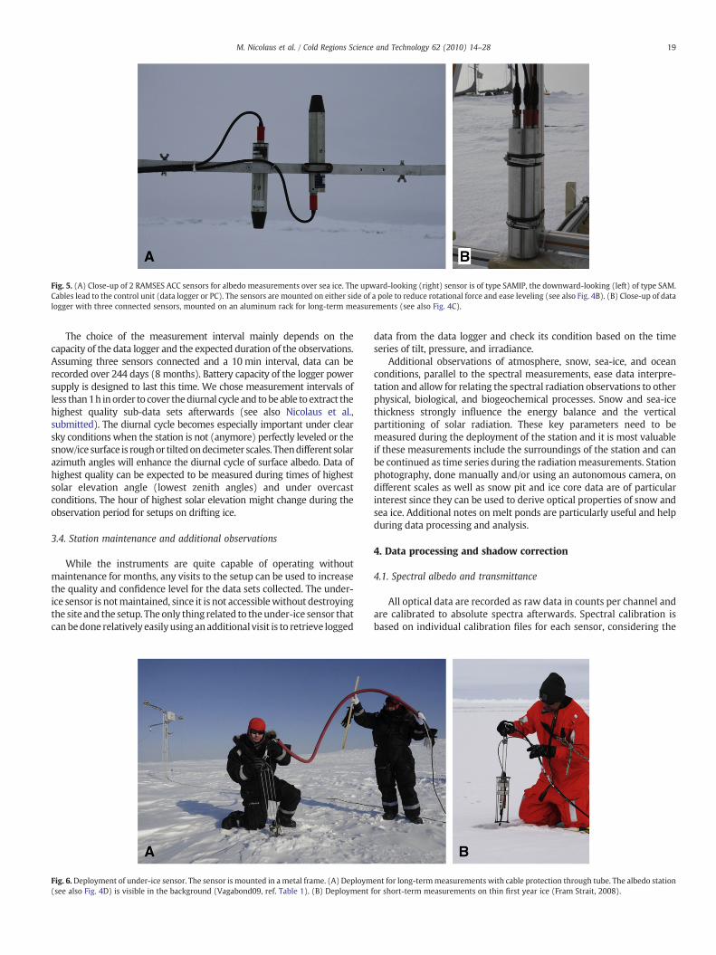
Fig. 5. (A) Close-up of 2 RAMSES ACC sensors for albedo measurements over sea ice. The upward-looking (right) sensor is of type SAMIP, the downward-looking (left) of type SAM.Cables lead to the control unit (data logger or PC). The sensors are mounted on either side of a pole to reduce rotational force and ease leveling (see also Fig. 4B). (B) Close-up of datalogger with three connected sensors, mounted on an aluminum rack for long-term measurements (see also Fig. 4C).


The choice of the measurement interval mainly depends on thecapacity of the data logger and the expected duration of the observations.Assuming three sensors connected and a 10 min interval, data can berecorded over 244 days (8 months). Battery capacity of the logger powersupply is designed to last this time. We chose measurement intervals ofless than1h inorder to cover thediurnal cycle and tobeable to extract thehighest quality sub-data sets afterwards (see also Nicolaus et al.,submitted). The diurnal cycle becomes especially important under clearsky conditions when the station is not (anymore) perfectly leveled or thesnow/ice surface is roughor tiltedondecimeter scales. Thendifferent solarazimuth angles will enhance the diurnal cycle of surface albedo. Data ofhighest quality can be expected to be measured during times of highestsolar elevation angle (lowest zenith angles) and under overcastconditions. The hour of highest solar elevation might change during theobservation period for setups on drifting ice.

3.4. Station maintenance and additional observations

While the instruments are quite capable of operating withoutmaintenance for months, any visits to the setup can be used to increasethe quality and confidence level for the data sets collected. The under-ice sensor is notmaintained, since it is not accessiblewithout destroyingthe site and the setup. Theonly thing related to theunder-ice sensor thatcanbedone relatively easilyusinganadditional visit is to retrieve logged

Fig. 6.Deployment of under-ice sensor. The sensor is mounted in ametal frame. (A) Deploym(see also Fig. 4D) is visible in the background (Vagabond09, ref. Table 1). (B) Deployment

data from the data logger and check its condition based on the timeseries of tilt, pressure, and irradiance.

Additional observations of atmosphere, snow, sea-ice, and oceanconditions, parallel to the spectral measurements, ease data interpre-tation and allow for relating the spectral radiation observations to otherphysical, biological, and biogeochemical processes. Snow and sea-icethickness strongly influence the energy balance and the verticalpartitioning of solar radiation. These key parameters need to bemeasured during the deployment of the station and it is most valuableif these measurements include the surroundings of the station and canbe continued as time series during the radiationmeasurements. Stationphotography, done manually and/or using an autonomous camera, ondifferent scales as well as snow pit and ice core data are of particularinterest since they can be used to derive optical properties of snow andsea ice. Additional notes on melt ponds are particularly useful and helpduring data processing and analysis.

4. Data processing and shadow correction

4.1. Spectral albedo and transmittance

All optical data are recorded as raw data in counts per channel andare calibrated to absolute spectra afterwards. Spectral calibration isbased on individual calibration files for each sensor, considering the

ent for long-termmeasurements with cable protection through tube. The albedo stationfor short-term measurements on thin first year ice (Fram Strait, 2008).


spectral calibration and sensitivity of each channel. Separate calibra-tion files for measurements in air and water are available for allsensors.

We interpolated spectra to a 1 nm grid before calculating ratios ofspectra from different sensors (albedo and transmittance), in order toaccount for sensor-dependent wavelength grids.Spectral albedo α(λ,t) was calculated as

α λ; tð Þ = FR λ; tð Þ= FI λ; tð Þ ð2Þ

and spectral transmittance T(λ,t) was calculated as

T λ; tð Þ = FT λ; tð Þ= FI λ; tð Þ ð3Þ

with wavelength λ and time t. Albedo data are linearly interpolatedbetween 748 and 773 nm, because of insufficient data quality in thiswavelength range (see Section 5.3).

4.2. Wavelength-integrated albedo and transmittance

In order to describe temporal changes, characterize general snowand ice properties, and to compare results with other sensors(especially broadband short-wave radiometers) wavelength-inte-grated, total, fluxes were calculated from the spectral data.

Total albedo αT(t) is calculated as

αT tð Þ = ∫α λ; tð ÞFI λ; tð Þdλ∫FI λ; tð Þdλ

ð4Þ

and total transmittance TT(t) equivalently as

TT tð Þ = ∫T λ; tð ÞFI λ; tð Þdλ∫FI λ; tð Þdλ

ð5Þ

Mean total albedoPαT and transmittance

PTT (over time) are calculated

from the time averages of the respective fluxes as

PαT =

∬FR λ; tð Þdλdt∬FI λ; tð Þdλdt

ð6Þ

and

PTT =

∬FT λ; tð Þdλdt∬FI λ; tð Þdλdt

ð7Þ

These wavelength-integrated fluxes differ from broadband mea-surements because RAMSES ACC sensors do not observe wavelengthslonger than 950 nm. Depending on cloud coverage, humidity, and solarzenith angle, the RAMSES ACC sensors cover between 70% and 90% ofthe incident short-wave radiation in the range from 350 to 2500 nm(compared to irradiance spectra by Grenfell and Perovich, 2004); thelarger fractions are obtained under cloudy skies since the clouds absorbmuch of the incident infrared light. These fractions are much higher inwater and under sea ice, due to the high absorption of water and ice inlonger wavelengths. Exact numbers depend on optical properties andthicknesses of snow, ice, and water.

Direct comparisons of albedo with total fluxes and broadbandmeasurements show that RAMSES ACC albedo is generally higher butexplains most of the temporal variability. Exact numbers depend onseason, with highest differences during summer, when near-infraredalbedo is especially low (Nicolaus et al., submitted).

4.3. Shadow correction

Shadows on sensors or on the observed surface that originate fromobstacles other than the setup itself can usually be avoided whenchoosing the site and the setup, thus they are not considered here. Butimpacts on the data causedby the rack itself cannot be avoided andneedto be accounted for during data processing. These impacts include thesetup shading the observed surface and restricting the field of view ofthe cosine receptors. Having a thorough description of the location, anddimensions of the support rack for the above-ice instruments makes itpossible to determine a good estimate of the corrections necessary toaccount for the various shadowing components: the portion of FR that iskept from reaching the downward-looking sensor due to the obstacles,the reduction of FR caused by the reduction of light incident on thesurface due to the obstacles, the reduction of FT caused by the reductionof light incident on the surface due to the obstacles, and (if the setupmust have obstacles above the incident sensor) the reduction in themeasured FI due to those obstacles. Impacts on FT and FI are notconsidered here, as they can usually be avoided through the design ofthe setup.

A set of Matlab routines was written to calculate the shadowcorrection for complex setups as accurately as possible. First, all surfacesthat make up the albedo setup are defined. Usually each object is madeupof six rectangular faces, though the facesmay be other shapes, and anobject may contain more or fewer faces (e.g., a cylinder may beapproximated as a polygon with many rectangular sides). Fig. 7 showsthe description of two racks used for data collection during Tara07 andBarrow08, which are shown in photographs in Fig. 4B–C.

Once the setup is described, the reduction it causes to the observedreflected irradiance is calculated, with the following assumptions: thesnow/ice surface is a Lambertian reflector and spatially uniform; theincident light is either isotropic or perfectly collimated; all parts of thesetup are perfectly black. The final assumption makes the result anupper limit on the correction. The assumption of isotropic incidence is areasonable approximation of cloudy skies, while an accurate correctionfor clear skies is more complicated, requiring a combination of theisotropic and direct incidence assumptions, in which the weighting ofthe twowould vary with wavelength and atmospheric conditions. Herewe focus on the case with isotropic incidence. A grid of points is createdon the surface around the setup, located every 15 cm in the twoarbitrarily chosen x and y directions. At each grid point, an angular gridof incidence angles (1°×1° in zenith and azimuth) is created. Eachincidence angle is tested to determine if it intersects any part of thesetup. If the intersection of the line with any one or more of the planeslies inside the face that defines the plane, then the incidence anglereceives light from the setup, not the sky. An integration over theunblocked incidence angles is performed, summing the incidentintensity (set to 1/π) times the cosine of the incident zenith angle (θi)times the element of solid angle (sin θi dθi dϕ). If all angles areunblocked, this gives an incident irradiance of 1, so the result here is thefraction of undisturbed incident irradiance that reaches each point onthe surface.

The final step in calculating the correction is to consider the viewfrom the downward-looking sensor. An angular grid of viewing angles(0.5×0.5° in zenith and azimuth) is created, then each viewing angle istested to determine if it sees the snowor part of the setup. If the viewingangle sees the setup, it is assumed no light is reaching the sensor fromthat viewing angle; otherwise, the intersection of the line with thesurface is found, and the observed intensity is set to f×(1/π), where f isthe fraction of incident flux reaching that point, interpolated from theresult of the calculation in the previous paragraph. This observedintensity, weighted by the cosine of the viewing zenith angle and theelement of solid angle, is then integrated over the unblocked angles. If fwere one everywhere (no incident light blocked from reaching thesurface) and no viewing angles intersected the setup, the observed fluxwould be 1, so the result here is the upwelling flux observed by the

Fig. 7. The racks from (A) Oden08 and (B) Tara07, as described in the shadow correctionroutines. Shadings illustrate separate objects that were defined and do not representreal colors. Note different scales in both plates.


sensor with the setup blocking light, as a fraction of the upwelling fluxthat would be observed with no objects blocking any light. The correct-ion for collimated incidence is carried out in a similar way, but thesurface grid points aremore closely spaced, and the surface brightness isbinary, receiving either the full incident irradiance or none at all (f iseither 1 or 0).

For the Tara07 rack, shown in Figs. 7A and 4C, the result indicatesthat, under isotropic incidence, the true albedo is 1.083 times themeasured albedo (the measured FR is 7.7% less than what it would bewithout the rack). For collimated incident light from a zenith angle of70°, the correction ranges from1.06 to 1.11 for different azimuth angles.By contrast, the correction for the tripod setup (Figs. 4B and 7B) is only1.029 (the measured FR is 2.8% less than what it would be without therack), for isotropic incidence and a height of the FR sensor of 1.0 mabovesurface.

The same correction was applied for FT, quantifying the amount oflight that is transmitted through the ice but blocked from reaching thesensor by the frame and the suspension (Fig. 6). The frame geometry isdescribed in the same way as the surface rack described above and thereference surface is the ice underside, instead of the snow/ice surface.The correction assumes isotropic light under the ice and ignores anycontribution from light coming from below. This assumption iscertainly less accurate than for the FR calculation because under-iceradiance field is anisotropic, with a strong vertical component. As mostof the obstacles, frame and cables, are located straight above the sensor,the result describes aminimum correction. For the presented frame, thetrue irradiance is 1.087 times larger than the measured signal (themeasured FT is 8.04% less than without the obstacles). Finally, allcorrections (for FT and FR) were applied as a wavelength- and time-independent factor on all spectra.

4.4. Correction for depth of the under-ice sensor

The under-ice sensor is not located directly under the ice, butapprox. 1 m of sea water is between the ice under side and the sensor.This distance allows the frame to hang under the ice without anycontact with the ice, also when ice thickness increases during theobservation period. This additional meter of water is not corrected forduring data processing, although it reduces the amount of lightmeasured at the sensor. So, it has to be considered for data analysisand interpretation (e.g. Nicolaus et al., submitted). This is because thespectral attenuation coefficient of sea water depends on variousaspects and is time dependent. Hence, accurate measurements wouldbe needed or alternatively literature values for sea water could beused, resulting in a very general correction. Future setups couldinclude two under-ice sensors at different depths close to each other,allowing for the derivation of the attenuation coefficient.

In contrast to this general depth correction, spectra can becorrectedmore reliably for a drop of the sensor during the observationperiod, as might result from changing ice conditions. We observedsuch a drop once in the setup at Tara07 (Nicolaus et al., submitted).The correction is based on the transmitted irradiance before (FT(λ,t0))and after (FT(λ,t0+dt)) the drop (at time t0), assuming that changesin FT are only related to the depth change and that all other factorsinfluencing FT are minor and can be neglected. This is especially thecase when the drop happens within a short time interval (dt). Thecorrected transmitted irradiance FTcorr(λ,t) can then be derived as

FTcorr λ; tð Þ = FT λ; t0ð Þ−FT λ; t0 + dtð Þz t0ð Þ−z t0 + dtð Þ * z tð Þ−z t0ð Þð Þ + FT λ; tð Þ ð8Þ

with wavelength λ, depth z and time t. This correction was performedfor the Tara07 data, when the sensor dropped by 0.65 m within 4 h(Nicolaus et al., submitted). In order to reduce the effect of short-termvariability FT(λ,t0) and FT(λ,t0+dt) were averaged over 12 h before t0and after t0+dt.

5. Application of the setup

5.1. Sample data set

Table 1 gives an overview of our existing data sets that werecollected with this setup and include simultaneous albedo andtransmittance observations spanningmore than 24 h. Beyond the listedmeasurements, the setup has been used for various shorter observa-tions, for example on ice stations during ship expeditions. In addition tothe spectral radiation data, other data sets of atmospheric andoceanographic as well as snow and sea-ice properties were collected.These data sets are also listed in Table 1. Results from the Tara07campaign can be found in Nicolaus et al. (submitted).

Herewe showdata collected onArctic sea ice during a drift station ofthe Swedish ice breakerOden, as part of the Arctic Summer CloudOceanStudy (ASCOS, hereafter: Oden08). Continuous (10 min. intervals)measurements lasted just over two weeks. In total, 2410 albedo and2325 transmittance spectra were recorded (the slightly shorter recordof transmittance is due to the more time-consuming retrieval of theunder-ice sensor). The stationdrifted in the area between theNorth Poleand Svalbard from 87°25′N, 005°54′W to 87°09′N, 010°18′W. Allmeasurements were performed during polar day with solar elevationangles (elevation angle=90° — zenith angle) between 5.5° and 16.1°.The observation period comprises 16 full diurnal cycles. The under-icesensor was installed 1.0 m under the sea ice. Initial ice thickness, snowthickness, and freeboard at the station were 1.54, 0.10, and 0.05 m,respectively. The station was visited daily to check for leveling andcondensation or icing on the sensors. In addition, observations of snowproperties and general meteorological conditions were performed.When installed, the station was oriented with the support arm


extending in the East–West direction (270°) and regular observationsshowed that the orientation varied between 260° and 290°, resultingfrom floe rotation around its vertical axis. Presented data are correctedfor shadoweffects on the sensors:measured FRwas estimated to be 2.8%too lowdue to the setup shading the surface andblocking reflected light;measured FTwas estimated to be8.04% too lowdue to the support framefor the underwater sensor blocking transmitted light.

5.2. Results of spectral albedo and transmittance

The entire system functioned as planned. Spectral albedo andtransmittance show the transition from summer to autumn conditionswith two distinct phases, before and after 24 Aug (Fig. 8), which can beidentified as the end of melting season and onset of freezeup for thestudy region in 2008. The rapid change from summer to autumnconditions was initiated through a distinct snowfall event, resulting inapproximately 8 cm of new snow.

Weather conditions were characterized by fog and temperaturesaround 0 °C duing the first 5 days (until 20 Aug) of the observationperiod. Themost siginficant event during this timewas a snowfall eventearly on 17 Aug, which can be clearly identified in both spectral albedoand transmittance (Fig. 8) and is shown in Fig. 11, too. Albedo increasedfrom values around 0.85 to over 0.90 at wavelengths between 350 and750 nm, while longer wavelengths were less affected. This was mostlikely due to the still warm and wet sea-ice surface, which was stillvisible through the new snow. Transmittance at 500 nm temporarily

Fig. 8. Time series of (A) spectral albedo and (B) spectral transmittance as measured durinlinearly interpolated between 748 and 773 nm(see also Fig. 10). No data processing or corr

decreased by 0.014 from 0.074 to 0.060 (on 17 Aug), before it increasedto its maximum of 0.093 late on 19 Aug. The wavelength-integratedmaximum transmittance amounted to 0.049. During times ofmaximumtransmittance, 5.8 Wm−2 were transmitted through the snow and seaice into the upper ocean. After the snowfall event and until 20 Aug,albedo decreased over all wavelengths again, to even lower values thanbefore the snowfall.

On 20 Aug, a snowfall event with large flakes, lasting approxi-mately 5 h (Fig. 11), increased albedo and decreased transmittancesignificantly. Additional snowfall afterwards can be recognized inboth albedo and transmittance time series. Surface freezeup startedon 20 Aug, and was supported by lower air temperatures on 21 Augand afterwards. Despite the lower temperatures, snow thicknessdecreased to around 1 cm on 22 Aug. As a consequence of surfacefreezeup and the heavy snowfall on 23/24 Aug, total albedo increasedby 0.06 from 0.86 (mean between 15 and 23 Aug) to 0.92 (meanbetween 24 Aug and 01 Sep) and the total transmittance decreased by50% from 0.030 to 0.015. Afterwards, neither albedo nor transmittancereturned to their earlier values.

An additional light snowfall event occurred on 25 Aug (Fig. 11).This event had no significant influence on albedo and transmit-tance on longer time scales and albedo returned to its previousvalues within 2 h. Snow thickness decreased to 3 to 4 cm by theend of the observation period. Finally, drizzle decreased the albedoagain on 31 Aug and 01 Sep, especially for wavelengths longer than600 nm.

g Oden08 (Table 1). Data are shown with 2 hour temporal resolution. Albedo data areection has been performed to treat albedo values N1, which are shown in white.

Fig. 9. Spectra of solar irradiance, measured with the described RAMSES ACC sensor during Oden08 (Fig. 8) and a mean spectrum for overcast conditions on Arctic sea ice re-plottedfrom Grenfell and Perovich (2004). RAMSES ACC data collected under overcast conditions are highlighted. To aid the comparison, all spectra are normalized to have a maximumspectral irradiance of one, and all are plotted with 1 nm spectral resolution.

Fig. 10. (A) Spectral albedo and (B) spectral transmittance measured with the described RAMSES ACC sensors during Oden08 (Fig. 8) and Tara07 (re-plotted from Nicolaus et al.,submitted). All spectra are plotted with a spectral resolution of 1 nm, as used for further analysis. Grey-shaded areas mark wavelength ranges where data were not used for analysesin these papers.


Fig. 11. Spectral albedo at 400 nm (α(400)) asmeasured during Oden08 (see also Table 1). Times of precipitation aremarked light and dark grey. Times of sensor cleaning and stationleveling are indicated with symbols on the x-axis. Albedo time series is shown in full temporal resolution of 10 min. Precipitation was derived from cloud radar data by MatthewShupe (U. of Colorado, USA), and classified into light (very light snow fall/crystals in the air) and strong (snow fall and rain) precipitation.


5.3. Data quality

For assessing the data quality of the applied RAMSES ACC sensorbeyond the presented calibrations and uncertainties given by themanufacturer, incident irradiance spectra are compared to referencespectra from literature (Grenfell and Perovich, 2004) (Fig. 9) and un-corrected albedo and transmittance spectra are presented anddiscussed(Fig. 10). For albedo, effects of sensor contamination byprecipitation arequantified based on Fig. 11. All comparisons and discussions are basedon the presented data set from Oden08. Additional results from Tara07are included to allow for more generalization (Fig. 10).

5.3.1. Quality of spectral irradianceThe measurements by Grenfell and Perovich (2004) (hereafter

GP04) were performed over sea ice under stable overcast conditionsclose to Barrow, Alaska. For their measurements, they used a FieldSpecPro FR (Analytic Spectral Devices, Boulder, USA) with a single cosinereceptor foreoptic and a wavelength range from 350 to 2500 nm. Thisinstrument consists of three spectral radiometers that are combinedinto one system, but here we consider only data from the first spec-trometer,measuring 350 to 1000 nm. The effective spectral resolution isgiven as 1.4 nm in this wavelength range, but interpolated to 1 nmresolution by the instrument's software (Kindel et al., 2001). Thespectrum fromGP04, see their Fig. 11, is an average of several measure-ments under similar conditions in order to achieve a representativespectrum for high latitude irradiance. This spectrum is compared withspectra measured with our system during times of highest solarelevation. Since absolute fluxes could not be compared due to differentsolar and atmospheric conditions, all spectra are normalized to have amaximum spectral irradiance of one.

Fig. 9 shows the comparison and highlights the RAMSES ACC spectramade under overcast conditions (on 16, 17, 18, 28, and 29 Aug), whichshould be most comparable to the GP04 spectrum. Both instrumentsshow the same characteristic features (absorption lines) of solarirradiance under overcast conditions. The smallest differences werefound for the measurement on 29 Aug, when the mean difference wasonly 0.01 and the correlation coefficient was 0.995. But also in general,the RAMSES ACC data agree well with those from GP04, especially forthe selected dates and for wavelengths shorter than 600 nm. However,most of the RAMSES ACC spectra show higher normalized fluxes thanthose from GP04. Most of the differences may be explained by differentatmospheric conditions, and some spectra may be additionallyinfluenced by precipitation. Due to the higher spectral resolution (1.0vs. 3.3 nm) and different wavelength grid, absorption lines are moredistinct in the GP04 than in the RAMSES ACC data.

5.3.2. Quality of spectral albedo and transmittanceSpectral albedo and transmittance were calculated from interpolated

(1 nm) irradiances based on Eqs. (2) and (3), taking the sensor-specificwavelength grids into account. In order to assess data quality of spectralalbedo and transmittance, daily spectra from times of highest solarelevation are shown in Fig. 10. Thequality of the albedo and transmittancevalues and spectral shapes cannot be discussed in general, as this wouldrequire comparative measurements from another instrument over andunder identical snow, sea-ice and atmospheric conditions. However,Fig. 10 shows that bothmeasurements (albedo and transmittance) resultin reasonable spectral shapes and absolute values for the given snow andice conditions. This should be expected, since the sensors performwell inmeasuring irradiance spectra (see above and Fig. 9) and hence it may beassumed that the general spectral characteristics and absolute fluxes oftheir quotients are also of high quality. Here we concentrate on qualityaspects regarding the use of two sensors with different wavelength gridsand regarding applications without or with only limited maintenance.

Compared with the generally good results, data quality seems tobe lower in three wavelength ranges, as highlighted in Fig. 10A. Forwavelengths between 320 and 350 nm, at the lower end of thespectral range, spectral albedo shows unexpected variability and ahigh noise level. In Oden08 data, albedo strongly decreases withwavelength while it increases with wavelength in the Tara07 data.Although most studies do not include wavelength below 350 or even400 nm, various studies indicate that snow and ice albedo increasesmoderately with wavelength or is rather constant over this wave-length interval (Perovich et al., 1998; Perovich et al., 2002a; Warren,1982; Warren and Brandt, 2008). Similar problems (high noise leveland unexpected variability) are also observed for wavelengths longerthan 920 nm. These values are also likely unrepresentative for thegiven surface properties. Hence, for further data processing, all albedospectra from RAMSES ACC sensors are restricted to wavelengthsbetween 350 and 920 nm.

The third obvious feature appears as spikes in the albedo spectrabetween 750 and 775 nm. These spikes result from the Oxygen (O2)absorption line around 760 nm (Fig. 9), which is sampled at slightlydifferent wavelengths by the two sensors due to their differentwavelength grids. In order to remove this effect, albedo data arelinearly interpolated between 748 and 773 nm. This effect is seen atother wavelengths as well (Fig. 10), as noise in the albedo spectra onscales of the spectral resolution, but it is most pronounced around theO2 line, where the irradiance changes rapidly with wavelength. Atother wavelengths, the effect is more obvious in the Oden08 than inthe Tara07 data, suggesting that this mainly depends on how similarthe wavelength grids of the two sensors are.


Data quality of spectral transmittance shows basically the samefeatures as spectral albedo, but atmospheric absorption lines play only aminor role, so that no similar interpolation is performed. Due to highnoise levels and less reliable data at both ends of the spectral range,transmittance data are also restricted to wavelengths between 350 and920 nm.

The presented data were measured at a maintained station, butquality issues such as clean sensors and tilt of the station still need to beconsidered. Having the manual observations, just makes them easier toquantify and correct. At regular inspections during the measurementphase (see also Fig. 11), no rime or other particles on the sensors wereobserved, except some moisture after a period of fog on 23 Aug. Thesnowfall events on17and23/24Augmust have temporarily covered theupward-looking irradiance sensor, but no snow was observed on thenext check afterwards. Additionally, the station was adjusted in height(to return the FR sensor to 1.0 m above surface) and re-leveled fourtimes during the observation period, basically to account for changingsnow thickness. On 16 Aug, an icicle was found hanging from thereflected irradiance sensor and was removed.

In order to estimate times and duration of radiation data that need tobe corrected or excluded, the full resolution albedo time series at400 nm is shown in Fig. 11. At this wavelength, the albedo of snow isonlyweakly dependent on grain size and liquidwater content (which isoften high on summer sea ice), and the albedo of new snow is expectedto be 0.98 (Warren, 1982). But here albedo values are below 0.98 for alltimes when reliable data are available. This is most likely due to the factthat the snow was not yet opitcally thick, and the darker sea ice stillinfluenced the albedo measurements (Wiscombe and Warren, 1980).The most significant variations in the time series occur around thestrong snowfall events on 16 and 23/24 Aug, when spectral albedovalues exceed 0.98 and, at times, 1.00 (Figs. 8A, 10, and 11). This impliesthat during times of snowfall, and for some time afterwards, snowaccumulation on theupward-looking sensor resulted inunderestimatedincident irradiances. Afternewsnowfall stopped,α(400)decreases frommaxima larger than 1.00 to 0.96 within 12 to 24 h (Fig. 11). During thesnow event on 20 Aug, α(400) increases, as the new snow increasessurface albedo, but measurements do not exceed reasonable albedovalues for new snow and there is no short-lived spike in the values.Hence, it appears that this snowfall had little or no effect on the sensors.Most of the light snowfall events seem to have no impact on the dataquality, and albedo values return to their original values within 2 h (e.g.29 Aug). Other short-term variability of α(400) might be related tochanges in surface properties, such as snow metamorphism or rimeformation, but are not discussed here.

6. Discussion and conclusions

Here we have introduced a setup of three sensors for synchronous,autonomous, continuous, and high temporal-resolution measure-ments of spectral albedo and transmittance of snow and sea ice.RAMSES ACC sensors were used for the first time for studies of snowand sea-ice properties. The system is suitable for high-quality spectralradiation studies over and under sea ice at manned and un-mannedstations, contributing to increasing our understanding of atmo-sphere–ice–ocean interaction processes during different seasons.

6.1. Data quality — spectral information

The sensor-specific calibration of the RAMSES ACC sensors resultssome data quality issues. For albedo and transmittance measurements,the wavelength range should be restricted to 350 to 920 nm, excludingthe ends of the nominal spectral range, where noise levels are higherand results seem less reliable. This restricted wavelength range is alsocloser to the given specification of the MMS1 (360 to 900 nm). Hence,the observed effects are most likely due to the sensor's sensitivity andcalibrations at the edges of the spectrum. Furthermore, lowerfluxes lead

to higher uncertainties under division, so these effects become mostobvious for albedo and transmittance. For albedo measurements,spectra should additionally be interpolated between 748 and 773 nm,where the absorption line of Oxygen (O2) is not sufficiently wellobserved. As albedo curves are close to linear over this shortwavelengthrange (Perovich, 1996; Perovich et al., 1998; Warren, 1982), these dataare linearly interpolated and only minor effects on results and dataquality are expected. Although it is not practical with the suggestedsetup, applications using only one sensor (e.g. flipping it around foralbedo measurements), could further increase the data quality, as thiseliminates effects of the sensor-specificwavelengthgrid and calibration.

RAMSES ACC sensors cover the most interesting part of thespectrum for the presented studies of physical properties of snow andsea ice, particularly when focusing on transmitted light. Under ice,almost all energy falls within the RAMSES ACC spectral range, since iceand water attenuate most of the solar energy at wavelengths longerthan 700 nm. Optional UV-sensors could extend the wavelengthrange towards smaller wavelengths, which could be advantageous forsome chemical and biological studies. Beyond the presented use, thegiven wavelength range also allows a separation of physical andbiological effects as well as advanced analyses, such as differentiationof species and pigments and estimation of biomass as a function oftime.

However, data quality descriptions in this study aremostly based onqualitative discussions and do not include direct comparisons withother sensors. More detailed studies on data quality of RAMSES ACCsensors, especially focusing on albedo and transmittance spectra, aresuggested and should include synchronous measurements with othersensor systems, includingwith a FieldSpec Pro FR, to our knowledge, themostwidely-used spectral radiometer for field studies in snow and sea-ice research (e.g. Ehnet al., 2008b;Gerlandet al., 1999; Light et al., 2008;Perovich, 2007), especially when focusing on maximizing data qualityand obtaining reference spectra (e.g. Grenfell and Perovich, 2008).Alternatively, sensors and solutions from Ocean Optics (Dunedin, USA)and Satlantic (Halifax, Canada) could be used for comparisons. Thesesensor systems might also be suitable to be used in similar setups.

The pressure measurements from the SAMIP sensors are accurateenough for underwater depth measurements, but not for monitoringatmospheric pressure. Tilt accuracies (1°) allow for good monitoring ofsensor tilt over time, but the values are not useful for leveling the setupat installation because the axes are not marked on the outside of thesensors' casing.

6.2. Data quality — cleanness of sensors

6.2.1. Ice and water on sensorsThe RAMSES ACC sensors were found to perform particularly well

with respect to contamination by ice and water. The sensors were notobserved to be affected by anymoisture or snow and did not have to becleaned during the entire summer season at Tara07 (Nicolaus et al.,submitted). This observation is based on daily visits. However, it cannotbe concluded that there was no contamination of the sensors at anytime, but rime or other moisture evaporated within short time periodsand before the next visit. During the presented observations at Oden08,the RAMSES ACC sensors were cleaned of snow or moisture 3 times in17 days. But also when they were not cleaned manually, measuredsignals returned to their expected values within short times as soon asprecipitation had stopped. Here we derived a time span of 2 to 12 h,depending on the strength of the prior snowfall (Fig. 11).

In contrast, standard pyranometers used for short-wave broad-band radiation measurements, needed to be cleaned under the sameconditions at least once a day during both campaigns. This differenceis assumed to be mainly related to the construction of the sensors.Dome sensors allow the accumulation of snow and moisture directlyon the glass dome above the sensor, and they hinder fast evaporation,since, by design, they are very poor absorbers of radiation. In contrast


the black, conic-shaped heads of the RAMSES ACC sensors allow a self-cleaning effect; the cosine collector (diffuser plate) is embedded intothe sensor's head, reducing accumulation and enhancing evaporationas soon as the sun warms the head and/or wind speeds up.

Summarizing, it may be concluded that RAMSES ACC sensorsrecovermuch faster from contamination by precipitation than sensorswith domes. Their design causes water and ice to naturally evaporatein a short time (here a few hours), but during and after heavy snowfallor rain, data are affected. An even larger and more long-lasting effecton data quality can be expected from freezing rain, which is known tocover any kind of instrument with an ice layer in short time. But thiseffect cannot be quantified because it has not yet been experiencedduring measurements with the presented sensors.

6.2.2. Biological impacts and sedimentationThe growth of biota on the under-ice sensor or on the underwater

frame is difficult to quantify because, with our present setup, it cannotbe monitored directly. Anyhow, it is known to reduce the amount oflight reaching the sensor. Even though the cosine receptors haveshown comparably resistant to contamination, the growth of algae orother microorganisms can most likely not be entirely preventedduring long-term installations. Moving devices that clean or cover thesensors while installed under the ice could reduce effects ofbiofouling. But such components also introduce additional challengesrelated to their functionality over long times and under the givenharsh conditions. Alternatively, the sensors could be coated by anti-foulingmaterials, but thesemust be tested to ensure they do not affectdata quality and optical properties.

Similarly, the accumulation of particles affects the measurements,with a different spectral signature. But sedimentation of particles canbe assumed to be of minor importance due to the small surface areaand the conic shape of the sensor and since those particles might bewashed away through mixing in the water column and currents.Further biological impacts could be marine mammals, and otheranimals in water, damaging under-ice setups, or polar bears, birds, orother animals living on the ice affecting surface measurements.

All these external, biological influences certainly depend on locationand duration of deployments. In order to reduce the likelihood of theseeffects, improvements to the setup, such as moving covers, can besuggested. Also complementary measurements may be performed toallow for adequate data corrections, but these steps are not realized yet.Nevertheless, those aspects would be of particular importance forseasonalmonitoring especially during seasons of high biological activityand primary production (e.g. Nicolaus et al., submitted), aswould be thecase on autonomously drifting platforms.

6.3. Three-sensor setup

One key feature of the presented setup is the simultaneousmeasurement of spectral albedo and transmittance. This enables directcomparison of both data sets and their common analysis. Thus, onlyminor assumptionshave to bemade to quantify the vertical and spectraldecomposition of solar radiation for the given snow/ice regime as afunction of time. Such consistent data sets are, furthermore,most usefulfor numerical simulations and model development.

The under-ice sensor is currently mounted in a frame, hangingstraight down under the bore hole. This design was chosen in order tokeep the setup as simple as possible, which is most desirable fordeployment inPolarRegions. Thedisadvantageof this setup is a relativelylarge shadowing effect on the sensor, which needs to be corrected forduring data processing. Using under-ice arms, as for example done byMobley et al. (1998), Gerland et al. (1999), and Light et al. (2008), wouldreduce this shadowing significantly, but also introduces new challengesto the stability of the setup and to the deployment itself. Nevertheless,such solutions should be considered in the future.

Even if the measurement site is selected to be as representative aspossible for a larger region during setup, this static setup cannotrepresent the usually high spatial variability of snow and ice propertiesondifferent scales (e.g. Eicken, 2003;Massomet al., 2001;Nicolaus et al.,submitted; Sturmet al., 2002). All data are spot data andmultiple setupswould be needed to quantify spatial variability. Furthermore, thepresented setup is hitherto restricted to certain ice regimes. Sea-icefeatures such as ridges melt ponds, new or thin ice, and thick ordeformed ice cannot be monitored due to technical restrictions. Butadditional measurement programs, including repeated transects ofradiation measurements or other physical properties of snow and ice,would allow generalizing findings from this setup to larger regions.

Quality and representativeness of the data set can be considerablyincreased by additional profile measurements of albedo and transmit-tance. Repeated transectswith additional sensors aremost valuable, butdepend on availability of personnel and accessibility of the station.Albedo profiles could be performed with comparably little effort, whiletransmittance profiles aremuchmore challenging and time-consuming.The latter would need multiple bore holes, divers, or pre-installedunder-ice constructions. Further developments of autonomousprofilingmethods above and under sea ice could support these additionalobservations.

Finally, instrumentation costs needs to be considered, especiallysince autonomous measurements have an increased risk of damage orloss of the instruments. This risk also includes the data, because all dataare stored locally on the ice. This could be improved by using a satellite-transmitting module instead of, or in parallel to, the local data logger.

6.4. Use in cold and remote regions

Its suitability for field work and long-term installations in coldregions is one of the most important criteria for the presented setup.First of all, it can be summarized that the design andmaterial of sensors,data loggers, cables, and connectorsperformedexceptionallywell underdifferent and challenging climatic conditions. The entire system wasfound to be well suited for the demonstrated field use. Especially thesensor and logger casings are excellent,with theirwaterproof (includingunderwater use) stainless steel casings.

Even though the design of the setup was made for stationarymeasurements, the tripod-based system is highly portable. All units aresufficiently light and compact to be easily and quickly set up by one ortwo persons, which is most valuable for short observation periods. Byitself, the albedo setup is very suitable for profile measurements, as itcan be easily moved and readjusted by two persons. The data-loggersystem is especially easy to handle, as it is very robust and sensors caneasily be added or changed withoutmodification. Having power supplyand data storage included in one unit, it supports autonomous andremote measurements. Sensors and loggers can be used without anypreconditioning (of instrument temperature). Dark currents arerecorded with each measurement, such that no on-site calibration orpre-heating/cooling is necessary. In all these aspects, the Trios systemstands out compared to most other radiometers.

During the Barrow09 measurements (Table 1 and Fig. 4A), no datawere recorded in the data logger. This was hitherto the only majorfailure andwasmost likely a consequence of a failure in power supply. Itis likely that the battery was initially defective or drained, but it is alsopossible that it failed due to exposure to the temperatures below−40 °C (installed in mid-winter, the Barrow09 station experienced thelowest temperatures the setup has thus far been used in). Additionaltests and repeated measurements during another Barrow fieldcampaign will be performed to determine if the data logger's batterypack will operate at extremely low temperatures.

As described above, the setup can be used in connection with a PCinstead of a data logger. This setup is allows immediate access andcontrol of measurements and data, unlike the data logger, whichneeds to be programmed and read out before and after


measurements. However, the PS (interface) box is not designed foroutdoor use under polar conditions and needs external power (12 VDC or between 85 and 265 V AC). Furthermore, long-term registra-tions with PC-connection have occasionally shown software-relatedproblems, making this configuration less reliable when immediateaccess and control is not planned or possible. The PC-setup is wellsuited for short stations and process studies, but less so for seasonalmonitoring.

6.5. Future improvements of the setup and method

In order to improve the data quality further and to standardize thedata sets, some aspects of the presented setup could be improved. Thereliability of the data logger (power failure) and PC data recording(software problems) should be further increased. The DSP data-loggerfunctionality could be improved by including a run-time control optionto check its status, battery, and memory level, as well as to allowdownloading or viewing data without interrupting data acquisition andreprogramming the logger. Integration into other observing systemswould be easier if the sensors could be controlled by other, widely-useddata loggers. From the different setup realizations (Fig. 4), the Barrow09setup is probably best suited for most applications. Its construction iscomparably simple and causes the least shadowing, but is also verystable and long-lasting. The white PVC eases its handling and absorbsvery little solar radiation.

Securing and stabilizing the rack under melting conditions can beimproved. So far, tension wires were fastened with ice screws, butthosemelted out of the ice early during the season. Evenmore difficultwould be deployments during summer, when constructions drilledinto the ice do not refreeze.

A camera, automatically taking photographs of the measurementsite, sensors, and sky conditions, would ease data processing signifi-cantly if no other observations and photographs are available. It couldadd valuable information about significant changes of snow and iceproperties, changes to the orientation of station, and any other eventsthat affect the measurements. It would, however, require additionalresources (power, data storage).

Snow thickness measurements are suggested as ultrasonicmeasurements right at the station, as realized during the measure-ments Barrow09 (Fig. 4A). These measurements give a continuousreading and can be extended by manual profiles and/or stake linesaround the station. Additional measurements of vertical profiles ofirradiance in the water under the ice could support data processing,because the extinction coefficient of water can be derived and supportthe depth correction of the under-ice sensor.

7. Perspectives

Beyond the above discussed improvements of data quality, thepresented setup could be extended by other sensor types in order toenhance the interdisciplinary description of atmosphere–ice–oceaninteraction. For example, biological studies could benefit from theinclusion of fluorescence sensors, chemical studies might favor anextension of the spectral range towards ultraviolet (UV) radiation,and oceanographic studies could use additional measurements oftemperature, salinity, and water velocities. Extending the setup withadditional RAMSES ACC sensors would enable studying spatial (lateraland vertical) variability of snow and sea-ice properties. Additionalsensors could be deployed around the station at the same depth underdifferent snow or ice regimes or in different depths, for exampleincluding those freezing into the ice as it grows in order to studyphysical ice parameters as a function of time in more detail.

In addition to the potential interdisciplinary work, further usesof data from this setup could include the retrieval of snow and iceproperties from their effect on the radiation measurements and thedevelopment and validation of numerical models and remote

sensing products. Although we presented the benefit of combiningmeasurements of spectral irradiance with those of snow and iceproperties, future applications of the presented setup may also beused to study physical snow and ice properties without specific in-situ measurements, by retrieving these properties from the radiationmeasurements. These data are most useful also for developing andvalidating numerical models and for calibration and validation ofremote sensing data. Studies based on optical remote sensing,especially using Moderate Resolution Imaging Spectroradiometer(MODIS) and Advanced Very High Resolution Radiometer (AVHRR)data (e.g. Willmes et al., 2009), are expected to be most interestingfor comparisons. Beyond this, data sets, gathered from the presentedsetup, have great potential to be used for biological and geochemicalstudies of sea ice (e.g. Ehn et al., 2008a; Mundy et al., 2005; Perovichet al., 1993). The presented setup could contribute to developing astandard for sensor technology and station setup, as it could be usedfor similar measurements at various places and times. Such astandard would ease comparative and joint analysis of data fromdifferent stations.

Including a satellite-transmitting unit, in addition to the setup'sexisting data logger, would reduce the risk of losing the data beforeretrieval and allow real-time data access. Receiving the data in realtime is also a very interesting option by itself and would be mostuseful when combined with other real-time observational data ormodel applications. Beyond this, an optional satellite-transmittingunit would allow advancing the system towards an independentbuoy system for sea-ice applications. Such an autonomously driftingstation would not need to be revisited for data and instrumentretrieval, but would mean losing the equipment, which is rathercostly with the current instrumentation. Spectral radiation measure-ments on buoys would be most efficient when deployed togetherwith other buoy systems, especially with an Ice Mass-balance Buoy(IMB, Richter-Menge et al., 2006). This would allow gathering mostcomprehensive data sets to study sea-ice mass and energy balancefrom remote sites.

Acknowledgements

Anders Sirevaag and Sara de la Rosa (University of Bergen,Norway) performed the Oden08 measurements, recorded additionalobservations, and regularlymaintained the station. This work is highlyappreciated. Matthew Shupe (University of Colorado, USA) kindlyprovided the precipitation data from this cruise. We thank the ASCOScoordinators Michael Tjernström and Caroline Leck and the crew ofthe Swedish ice breaker Oden for supporting these measurementsand for their cooperation. The work by Kristen Fossan (NorwegianPolar Institute, Tromsø) to manufacture different elements for thesetups and that by Chris Petrich (University of Alaska, Fairbanks,USA) to construct the PVC rack used in Barrow was most importantfor developing the presented setups. We highly acknowledge thecontribution of Christina A. Pedersen (Norwegian Polar Institute,Tromsø) to many discussions on the sensors and their data quality.We thank Rüdiger Heuermann and his colleagues from Trios,Oldenburg, Germany for their support of the RAMSES ACC sensorsand DSP data loggers. The authors wish to acknowledge thecontribution of two anonymous reviewers, which helped to improvethe manuscript. This study was funded through the DAMOCLES(Developing Arctic Modeling and Observing Capabilities for Long-term Environmental Studies) project, which is financed by theEuropean Union, and by the Norwegian Research Council throughthe IPY project iAOOS Norway — Closing the Loop (grant number176096/S30). Additional funding was received through the NorClimproject, financed in the Norklima program of the Norwegian ResearchCouncil as well as funding of the Norwegian Polar Institute and itsCentre for Ice, Climate and Ecosystems.


References

Allison, I., et al., 1993. East Antarctic sea ice: albedo, thickness distribution, and snowcover. J. of Geophys. Res.—Oceans 98 (C7), 12,417–12,429.

Banks, C.J., et al., 2006. Measurement of sea-ice draft using upward-looking ADCP on anautonomous underwater vehicle. Ann. Glaciol. 44, 211–216.

Boe, J.L., et al., 2009. September sea-ice cover in the Arctic Ocean projected to vanish by2100. Nature Geosci. 2 (5), 341–343.

Brandt, R.E., et al., 2005. Surface albedo of the Antarctic sea ice zone. J. Climate 18 (17),3606–3622.

Ehn, J.K., et al., 2008a. Bio-optical and structural properties inferred from irradiancemeasurements within the bottommost layers in an Arctic landfast sea ice cover.J. Geophys. Res. 113 (C03S03). doi10.1029/2007JC004194.

Ehn, J.K., et al., 2008b. Inference of optical properties from radiation profiles withinmelting landfast sea ice. J. Geophys. Res. 113 (C09024). doi10.1029/2007JC004656.

Eicken, H., 2003. From themicroscopic to themacroscopic to the regional scale: growth,microstructure and properties of sea ice, in Sea ice. In: Thomas, D., Dieckmann, G.S.(Eds.), An Introduction to Its Physics, Biology, Chemistry and Geology. BlackwellScience, Oxford, UK.

Ficek, D., et al., 2004. Spectra of light absorption by phytoplankton pigments in theBaltic; conclusions to be drawn from a Gaussian analysis of empirical data.Oceanologia 46 (4), 533–555.

Frolov, I.E., et al., 2005. Results from the Russian drifting stations. The Arctic BasinSpringer,Berlin.

Gascard, J.-C., et al., 2008. Exploring Arctic transpolar drift during dramatic sea iceretreat. Eos Transactions 89 (3), 21–28.

Gerland, S., et al., 1999. Physical properties, spectral reflectance and thicknessdevelopment offirst year fast ice inKongsfjorden, Svalbard. PolarRes. 18 (2), 275–282.

Grenfell, T.C., Maykut, G.A., 1977. The optical properties of ice and snow in the Arcticbasin. J. Glaciol. 18, 445–463.

Grenfell, T.C., Perovich, D.K., 1984. Spectral albedos of sea ice and incident solarirradiance in the southern Beaufort Sea. J. Geophys. Res. 89 (C3), 3573–3580.

Grenfell, T.C., Perovich, D.K., 2004. Seasonal and spatial evolution of albedo in a snow–ice–land–ocean environment. J. Geophys. Res. 109 (C1). doi10.1029/2003JC001866.

Grenfell, T.C., Perovich, D.K., 2008. Incident spectral irradiance in the Arctic Basin duringthe summer and fall. J. of Geophys. Res.—Atmospheres 113 (D12), 13.

Grenfell, T.C., et al., 2006. Spectral transmission and implications for the partitioning ofshortwave radiation in arctic sea ice. Ann. Glaciol. 44, 1–6.

Heege, T., et al., 2003. Mapping of Submerged Aquatic Vegetation with a PhysicallyBased Process Chain, Paper Presented at Proceedings of Remote Sensing. TheInternational Society for Optical Engineering, Barcelona, Spain.

Jin, M., et al., 2006. Controls of the landfast ice–ocean ecosystem offshore Barrow, Alaska.Ann. of Glaciol. 44, 63–72.

Kindel, B.C., et al., 2001. Direct solar spectral irradiance and transmittance measure-ments from 350 to 2500 nm. Appl. Optics 40 (21), 3483–3494.

Lavoie, D., et al., 2005. Modeling ice algal growth and decline in a seasonally ice-coveredregion of the Arctic. J. of Geophys. Res.—Oceans 110 (C11), 17 Resolute Passage,Canadian Archipelago.

Light, B., et al., 2008. Transmission and absorption of solar radiation byArctic sea ice duringthe melt season. J. Geophys. Res. 113 (C03023). doi10.1029/2006JC003977.

Massom, R.A., et al., 2001. Snow on Antarctic sea ice. Rev. Geophys. 39 (3), 413–445.

Mobley, C.D., et al., 1998. Modeling light propagation in sea ice. IEEE Transactions onGeoscience and Remote Sensing 36 (5), 1743–1749.

Mundy, C.J., et al., 2005. Variability of snowand ice thermal, physical and optical propertiespertinent to sea ice algae biomass during spring. J. Mar. Syst. 58, 107–120.

Mundy, C.J., et al., 2007. Influence of snow cover and algae on the spectral dependenceof transmitted irradiance through Arctic landfast first-year sea ice. J. Geophys. Res.112 (C3). doi10.1029/2006JC003683.

Nicolaus, M., et al. (submitted), Seasonality of spectral albedo and transmissivity asobserved in the Arctic Transpolar Drift in 2007, Journal of Geophysical Research.

Nicolaus,M., et al., 2009. Evolutionoffirst-year and second-year snowproperties on sea icein the Weddell Sea during spring–summer transition. J. Geophys. Res. 114 (D17109).

Odermatt, D., et al., 2008. Water quality monitoring for Lake Constance with aphysically based algorithm for MERIS data. Sensors 8 (8), 4582–4599.

Perovich, D.K., 1996. The Optical Properties of Sea Ice. CRREL, Hanover, USA.Perovich, D.K., 2005. On the aggregate-scale partitioning of solar radiation in Arctic sea

ice during the Surface Heat Budget of the Arctic Ocean (SHEBA) field experiment.J. Geophys. Res. 110 (C3). doi10.1029/2004JC002512.

Perovich, D.K., 2007. Light reflection and transmission by a temperate snow cover.J. Glaciol. 53 (181), 201–210.

Perovich, D.K., et al., 1993. Biooptical observations of 1st-year arctic sea-ice. Geophys.Res. Lett. 20 (11), 1059–1062.

Perovich, D.K., et al., 1998. Variability in Arctic sea ice optical properties. J. of Geophys.Res.—Oceans 103 (C1), 1193–1208.

Perovich, D.K., et al., 2002a. Seasonal evolution of the albedo of multiyear Arctic sea ice.J. Geophys. Res. 107 (C10). doi10.1029/2000JC000438.

Perovich, D.K., et al., 2002b. Aerial observations of the evolution of ice surfaceconditions during summer. J. Geophys. Res. 107 (C10). doi10.1029/2000JC000449.

Richter-Menge, J., et al., 2006. Icemass-balance buoys: a tool formeasuring and attributingchanges in the thickness of the Arctic sea-ice cover. Ann. Glaciol. 44, 205–210.

Sturm, M., et al., 2002. Winter snow cover on the sea ice of the Arctic Ocean at theSurface Heat Budget of the Arctic Ocean (SHEBA): temporal evolution and spatialvariability. J. Geophys. Res. 107 (C10). doi10.1029/2000JC000400.

Timmermans, K.R., et al., 2008. In situ and remote-sensed chlorophyll fluorescence asindicator of the physiological state of phytoplankton near the Isles Kerguelen(Southern Ocean). Polar Biol. 31 (5), 617–628.

Vihma, T., et al., 2009. Radiative and turbulent surface heat fluxes over sea ice in thewestern Weddell Sea in early summer. J. Geophys. Res. 114 (C04019). doi10.1029/2008JC004995.

Wang, M.Y., Overland, J.E., 2009. A sea ice free summer Arctic within 30 years? Geophys.Res. Lett. 36.

Warren, S.G., 1982. Optical properties of snow. Rev. Geophys. Space Phys. 20 (1), 67–89.Warren, S.G., Brandt, R.E., 2008. Optical constants of ice from the ultraviolet to the

microwave: a revised compilation. J. of Geophys. Res.—Atmospheres 113 (D14).Weeks, W.F., Ackley, S.F., 1986. The growth, structure and properties of sea ice. In:

Untersteiner, N. (Ed.), The Geophysics of Sea Ice. Plenum Press, New York, pp. 9–164.Willmes, S., et al., 2009. Observing snowmelt dynamics on fast ice in Kongsfjorden/

Svalbard with NOAA/AVHRR data and field measurements. Polar Res. 28, 203–213.Wiscombe, W.J., Warren, S.G., 1980. A model for the spectral albedo of snow I: pure

snow. J. of Atmospheric Sci. 37, 2712–2733.Zeebe, R.E., et al., 1996. Modeling the heating and melting of sea ice through light

absorption by microalgae. J. Geophys. Res. 101 (C1), 1163–1181.

Cold Regions Science and Technology - AWIepic.awi.de/22031/1/Nic2010b.pdf · A modern concept for...

Documents

Transcript of Cold Regions Science and Technology - AWIepic.awi.de/22031/1/Nic2010b.pdf · A modern concept for...