Cognitive satellite communications and representation ...

University of LouisvilleThinkIR: The University of Louisville's Institutional Repository

Electronic Theses and Dissertations

8-2019

Cognitive satellite communications andrepresentation learning for streaming and complexgraphs.Wenqi LiuUniversity of Louisville

Follow this and additional works at: https://ir.library.louisville.edu/etdPart of the Digital Communications and Networking Commons, and the Systems and

Communications Commons

This Doctoral Dissertation is brought to you for free and open access by ThinkIR: The University of Louisville's Institutional Repository. It has beenaccepted for inclusion in Electronic Theses and Dissertations by an authorized administrator of ThinkIR: The University of Louisville's InstitutionalRepository. This title appears here courtesy of the author, who has retained all other copyrights. For more information, please [email protected].

Recommended CitationLiu, Wenqi, "Cognitive satellite communications and representation learning for streaming and complex graphs." (2019). ElectronicTheses and Dissertations. Paper 3272.https://doi.org/10.18297/etd/3272

https://ir.library.louisville.edu/?utm_source=ir.library.louisville.edu%2Fetd%2F3272&utm_medium=PDF&utm_campaign=PDFCoverPages

https://ir.library.louisville.edu/etd?utm_source=ir.library.louisville.edu%2Fetd%2F3272&utm_medium=PDF&utm_campaign=PDFCoverPages

https://ir.library.louisville.edu/etd?utm_source=ir.library.louisville.edu%2Fetd%2F3272&utm_medium=PDF&utm_campaign=PDFCoverPages

http://network.bepress.com/hgg/discipline/262?utm_source=ir.library.louisville.edu%2Fetd%2F3272&utm_medium=PDF&utm_campaign=PDFCoverPages



https://doi.org/10.18297/etd/3272

mailto:[email protected]

COGNITIVE SATELLITE COMMUNICATIONS ANDREPRESENTATION LEARNING FOR STREAMING AND COMPLEX

GRAPHS

By

Wenqi LiuB.S., Donghua University, 2011

M.S., Stevens Institute of Technology, 2013

A DissertationSubmitted to the Faculty of the

J. B. Speed School of Engineering of the University of Louisvillein Partial Fulfillment of the Requirements

for the Degree of

Doctor of Philosophy in Electrical Engineering

Department of Electrical & Computer EngineeringUniversity of Louisville

Louisville, Kentucky

August 2019

COGNITIVE SATELLITE COMMUNICATIONS ANDREPRESENTATION LEARNING FOR STREAMING AND COMPLEX

GRAPHS

By

Wenqi LiuB.S., Donghua University, 2011

M.S., Stevens Institute of Technology, 2013

A Dissertation Approved On

June 24, 2019

by the following Dissertation Committee:

Hongxiang Li, Dissertation Director

Jacek Zurada

Andre J Faul

Lihui Bai

ii

DEDICATION

This dissertation is dedicated to all

who love, support and help human beings to make the earth a better place for us.

iii

ACKNOWLEDGMENTS

Firstly, I would like to thank my advisor, Dr. Hongxiang Li, Associate Professor,

Department of Electrical and Computer Engineering at the University of Louisville, for his

guidance, knowledge and patience during this academic journey.

I also would like to express my appreciation to my committee, Dr. Jacek Zurada,

Dr. Andre J Faul, and Dr. Lihui Bai for agreeing to serve on the dissertation committee. I

am deeply grateful for their encouragements and suggestions.

I would like to extend my grateful to my supervisor Dr. Bin Xie for his supporting

and collaboration during my internship at InfoBeyond Tech.

I would like to acknowledge my colleagues, Chen Cao, Xiaohui Zhang and Ruixuan

Han for their supports during the research. At last, special thanks to my family for their

great supports, wise counsel and sympathetic ear. Their love is always with me.

iv

ABSTRACT

COGNITIVE SATELLITE COMMUNICATIONS AND REPRESENTATION

LEARNING FOR STREAMING AND COMPLEX GRAPHS

Wenqi Liu

June 24, 2019

This dissertation includes two separate topics. The first topic studies a promising

dynamic spectrum access algorithm that improves the throughput of satellite

communication (SATCOM) under the uncertainty environment. The other topic

investigates real-time distributed representation learning for streaming and complex

networks.

1 Cognitive Satellite Communications

Dynamic spectrum access (DSA) allows a secondary user to access the spectrum holes

that are not occupied by primary users. However, DSA is normally operated under

uncertainty in a complex SATCOM environment, which could cause more spectrum

sensing errors or even service disruption. In this case, DSA requires a decision-making

process to optimally determine which channels to sense and access. To this end, I propose

a solution that addresses the uncertainty in SATCOM to maximize the system throughput.

Specifically, the DSA decision making process is formulated as a Partially Observable

Markov Decision Process (POMDP) model. Simulation results prove the effectiveness of

our proposed DSA strategy.

v

2 Distributed Real-time Representation Learning of Large Networks

Large-scale networks have attracted significant amount of attentions to extract and

analyze the hidden information from big data. In particular, graph embedding learns the

representations of the original network in a lower vector space while maximally

preserving the original structural information and the similarity among nodes. I propose a

real-time distributed graph embedding algorithm (RTDGE) which is capable of

distributively embedding the streaming graph data by combining a novel edge partition

approach and an incremental negative sample approach. Furthermore, a real-time

distributed streaming data processing platform is prototyped based on Kafka and Storm.

On this platform, real-time Twitter network data can be retrieved, partitioned and

processed for state-of-art tasks including synonymic user detection, community

classification and visualization.

For complex knowledge graphs, existing works cannot capture the complex

connection patterns and never consider the impacts from complicated relations, due to the

unquantifiable relationships. In this dissertation, a novel hierarchical embedding

algorithm is proposed to hierarchically measure the structural similarities and the impacts

from relations by constructing a multi-layer graph. Then an advanced representation

learning model is designed based on an entity’s context, which is generated by taking

random walks on the multi-layer content graph. Experimental results show that our

proposed model outperforms the state-of-the-art techniques.

vi

TABLE OF CONTENTS

Page

ACKNOWLEDGMENTS iv

ABSTRACT v

LIST OF TABLES xLIST OF FIGURES xi

CHAPTER

I INTRODUCTION 1

A Introduction on Efficient and Robust DSA Algorithm for SATCOM . 1

1 Dynamic Spectrum Access . . . . . . . . . . . . . . . . . . . 1

2 Types of Uncertainty in DSA . . . . . . . . . . . . . . . . . . 2

3 Related Work - Dynamic Spectrum Access . . . . . . . . . . 4

B Introduction on Graph Analysis and Embedding Algorithms . . . . . 5

1 Real-time Distributed Graph Embedding . . . . . . . . . . . . 6

2 Related Work - Graph Embedding . . . . . . . . . . . . . . . 8

3 Hierarchical Structural Embedding of Knowledge Graph . . . 9

4 Related Work - Knowledge Graph Embedding . . . . . . . . . 12

C Outline . . . . . . . . . . . . . . . . . . . . . . . . . . . . . . . . . 14

II EFFICIENT AND ROBUST DYNAMIC SPECTRUM ACCESS UNDER

UNCERTAINTY (ERDSAU) ALGORITHM FOR SATCOM 16

A Problem Significance, Motivations . . . . . . . . . . . . . . . . . . . 17

B Proposed Innovations . . . . . . . . . . . . . . . . . . . . . . . . . . 22

C System Model and Mathematical Formulation For ERDSAU . . . . . 24

1 Network Model . . . . . . . . . . . . . . . . . . . . . . . . . 25

2 Dynamic Spectrum Access (DSA) Model . . . . . . . . . . . 26

vii

3 Markov Process and Uncertainty . . . . . . . . . . . . . . . . 27

D LEO-Oriented Spectrum Sensing (LOSS) Algorithm . . . . . . . . . 30

1 LEO Spectrum Sensing . . . . . . . . . . . . . . . . . . . . . 31

E Key ERDSAU Notations . . . . . . . . . . . . . . . . . . . . . . . . 32

III DISTRIBUTED GRAPH PARTITION AND EMBEDDING ON LARGE-

SCALE STREAMING NETWORK 34

A Mathematical Model . . . . . . . . . . . . . . . . . . . . . . . . . . 34

1 Problem Formulation . . . . . . . . . . . . . . . . . . . . . . 35

B Real-time Distributed Graph Partition and Embedding . . . . . . . . 37

1 Graph Partition . . . . . . . . . . . . . . . . . . . . . . . . . 37

2 Dynamic Graph Embedding . . . . . . . . . . . . . . . . . . 41

3 Heuristic Global Aggregation . . . . . . . . . . . . . . . . . 43

C Experiments . . . . . . . . . . . . . . . . . . . . . . . . . . . . . . 45

1 System Setup . . . . . . . . . . . . . . . . . . . . . . . . . . 45

2 Graph Partition . . . . . . . . . . . . . . . . . . . . . . . . . 47

3 Dynamic Graph Embedding . . . . . . . . . . . . . . . . . . 48

4 Multi-label Classification . . . . . . . . . . . . . . . . . . . . 49

5 Link Prediction . . . . . . . . . . . . . . . . . . . . . . . . . 55

6 Scalability . . . . . . . . . . . . . . . . . . . . . . . . . . . . 56

IV REAL-TIME DEEP ANALYSIS OF TWITTER NETWORK 59

A Real-time Complex Twitter Network Extraction . . . . . . . . . . . . 62

1 Fundamental Graphs . . . . . . . . . . . . . . . . . . . . . . 63

2 Complex Graph Generation . . . . . . . . . . . . . . . . . . 64

B Results . . . . . . . . . . . . . . . . . . . . . . . . . . . . . . . . . 67

1 System Setup . . . . . . . . . . . . . . . . . . . . . . . . . . 67

2 Twitter Network Analysis . . . . . . . . . . . . . . . . . . . 68

V HIERARCHICAL STRUCTURE EMBEDDING OF KNOWLEDGE

GRAPH 72

viii

A System Model . . . . . . . . . . . . . . . . . . . . . . . . . . . . . 73

1 Scale-free Network . . . . . . . . . . . . . . . . . . . . . . . 73

2 Mathematical Definitions . . . . . . . . . . . . . . . . . . . . 74

3 Structural Distance Calculation . . . . . . . . . . . . . . . . 75

4 Relation Similarity Calculation . . . . . . . . . . . . . . . . . 77

5 Structural Graph Creation . . . . . . . . . . . . . . . . . . . 78

6 Knowledge Path Generation . . . . . . . . . . . . . . . . . . 79

7 Latent Representation Learning . . . . . . . . . . . . . . . . 80

8 Complexity and optimization . . . . . . . . . . . . . . . . . . 82

B Implementation and Experiments . . . . . . . . . . . . . . . . . . . 83

1 Implementation . . . . . . . . . . . . . . . . . . . . . . . . . 84

2 Data Sets . . . . . . . . . . . . . . . . . . . . . . . . . . . . 84

3 Entity Prediction . . . . . . . . . . . . . . . . . . . . . . . . 85

4 Multi-relations Prediction . . . . . . . . . . . . . . . . . . . 87

5 Triple Detection . . . . . . . . . . . . . . . . . . . . . . . . . 88

6 Scalability . . . . . . . . . . . . . . . . . . . . . . . . . . . . 89

VI CONCLUSION AND FUTURE WORK 91

A Conclusion . . . . . . . . . . . . . . . . . . . . . . . . . . . . . . . 91

B Future Work . . . . . . . . . . . . . . . . . . . . . . . . . . . . . . 93

REFERENCES 94

CURRICULUM VITAE 100

ix

LIST OF TABLES

TABLE Page

1 ERDSAU Notations . . . . . . . . . . . . . . . . . . . . . . . . . . . . . . 33

2 Data sets used for experiments in Section IV. . . . . . . . . . . . . . . . . 45

3 Multi-label classification results of BlogCatalog. . . . . . . . . . . . . . . 51

4 Multi-label classification results of Wikipedia. . . . . . . . . . . . . . . . . 52

5 Multi-label classification results of YouTube. . . . . . . . . . . . . . . . . 53

6 Performance evaluation w.r.t. dimensionality. . . . . . . . . . . . . . . . . 56

7 Performance evaluation w.r.t. dimensionality. . . . . . . . . . . . . . . . . 58

8 Generated complex graphs . . . . . . . . . . . . . . . . . . . . . . . . . . 68

9 Closest Twitter users of realDonaldTrump . . . . . . . . . . . . . . . . . . 70

10 Closest nodes detection . . . . . . . . . . . . . . . . . . . . . . . . . . . . 71

11 Compositional Representation Operator . . . . . . . . . . . . . . . . . . . 83

12 Data Sets . . . . . . . . . . . . . . . . . . . . . . . . . . . . . . . . . . . 84

13 Entity Prediction. . . . . . . . . . . . . . . . . . . . . . . . . . . . . . . . 85

14 Entity Prediction by Relation Types on FB38k . . . . . . . . . . . . . . . . 86

15 Hits@10(%) on FB38k . . . . . . . . . . . . . . . . . . . . . . . . . . . . 87

16 Multi-relation Prediction. . . . . . . . . . . . . . . . . . . . . . . . . . . . 88

17 Triple Classification . . . . . . . . . . . . . . . . . . . . . . . . . . . . . . 89

x

LIST OF FIGURES

FIGURE Page

1 Cognitive Satellite System Model . . . . . . . . . . . . . . . . . . . . . . 2

2 Edge Partition. . . . . . . . . . . . . . . . . . . . . . . . . . . . . . . . . 38

3 Subgraph Size Stand Deviation Evaluation. . . . . . . . . . . . . . . . . . 46

4 Maximum Subgraph Size. . . . . . . . . . . . . . . . . . . . . . . . . . . 46

5 Original Les Miserables network at (a) T = ti, (b) T = tj , (c) T = tk. . . . 47

6 Dynamic graph embedding results. . . . . . . . . . . . . . . . . . . . . . . 50

7 Link prediction results using weighted-L1 operator. . . . . . . . . . . . . . 54

8 Link prediction results using weighted-L1 operator. . . . . . . . . . . . . . 54

9 Micro-F1 Performance evaluation w.r.t. # computing nodes. . . . . . . . . 56

10 Macro-F1 Performance evaluation w.r.t. # computing nodes. . . . . . . . . 57

11 Speed up w.r.t Number of Partitions . . . . . . . . . . . . . . . . . . . . . 58

12 An example of the complex graph generation. . . . . . . . . . . . . . . . . 66

13 Distance between realDonaldTrump and his friends under policy∗1),

policy∗2) and policy∗3), respectively. . . . . . . . . . . . . . . . . . . . . . . 69

14 The distribution of entities appearing in random walks in FB15k follows a

similar power-law distribution as in Blog data social network. . . . . . . . . 73

15 Knowledge Graph. . . . . . . . . . . . . . . . . . . . . . . . . . . . . . . 75

16 Construction of Hierarchy Graph M . . . . . . . . . . . . . . . . . . . . . . 78

17 Scalability of Execution Time . . . . . . . . . . . . . . . . . . . . . . . . 90

xi

CHAPTER I

INTRODUCTION

A Introduction on Efficient and Robust DSA Algorithm for SATCOM

1 Dynamic Spectrum Access

Due to the spectrum scarcity, Dynamic Spectrum Access (DSA) becomes a desirable

technology to improve the utilization of electromagnetic spectrum for a SATCOM system.

It provides the capability that allows a Low Earth Orbit (LEO) in a SATCOM system to

dynamically use free channels that are not occupied by Geosynchronous (GEO) satellites

to augment the channel utilization. DSA has been extensively investigated in the last few

years [1]-[2] for CR (Cognitive Radio) networks. However, most of the DSA approaches

are developed for terrestrial communications without addressing the unique challenges in

a SATCOM environment and these challenges include the error-prone spectrum sensing,

the high mobility, the large GEO and LEO coverage, and a long signal delay due to long

distance signal propagation. Fig. 1 illustrates a SATCOM system where a LEO moves in

and exits the GEO coverage subsequently. The high LEO movement (i.e., about 17,000

MPH) degrades the reliability of the spectrum detection. When a LEO is moving close

to the edge of the GEO primary beam, its spectrum sensing results are not reliable and

change drastically in a very short time. The error probability of the spectrum sensing

varies with the GEO and LEO relative locations as well as the LEO mobility. In addition,

1

Cognitive Satellite User

GEO Satellite Earth Station

LEO Satellite Beam Spot

Inter Satellite Link

GEO Satellite Beam Spot

Figure 1: Cognitive Satellite System Model

GEOs and LEOs are operated in a hostile environment which is subjected to the adversarial

interference. Strong interference could result in a high misdetection probability. However,

most of the current DSA approaches, e.g., [3]-[4], are mainly developed for a relative static

environment where the secondary users are fixed or moving with a low speed in a small

geographic area, compared to the LEO’s mobility. On the other hand, the LEO spectrum

sensing suffers from weak GEO signals and long delay due to a long distance of the GEO

signal propagation.

Decision-making is a problem to determine which channels to sense and which

channels to access in a uncertainty environment. Specifically, the decision making for a

cognitive SATCOM should be conducted under three types of uncertainty.

2 Types of Uncertainty in DSA

• Uncertainty of sensing channels: A LEO is unable to detect all spectrum channels.

In other words, it only detects at most L out of N channels (L < N ) for a given time

instant. A sensing strategy is needed to decide which L channels to sense to achieve

a high probability of finding the GEO idle channels;

• Uncertainty of sensed status: The spectrum status may not be accurately sensed by a

2

LEO and the sensing results may have a high false alarm probability and a large miss

detection probability. For example, the probability of false alarm could be very high

(e.g., 30% or more) when external interference occurs;

• Uncertainty of spectrum access: Upon the high false alarm probability, it is a

problem to determine the optimal channel for LEO to access which achieves a high

data delivery ratio without collisions with the primary users.

With the consideration of the uncertainty in a SATCOM environment, this

dissertation proposal presents an approach to optimize the spectrum sensing and decision

making strategies for the purpose of improving the SATCOM spectrum utilization.

Specifically, we formulate the spectrum sensing and access under the uncertainty as a

problem of Partially Observable Markov Decision Process (POMDP). In the POMDP

problem, the partial observation indicates that a secondary user, e.g., LEO, is only able to

partially observe the underlying states of the primary channels. Meanwhile, the sensing

errors could occur in the partially observed spectrum band. Our approach in this paper has

the following contributions:

• GEO-oriented Spectrum Sensing: The spectrum sensing approach is studied to

improve the LEO sensing capability to detect the GEO spectrum holes. Our sensing

approach uses GEO signal-oriented cyclostationary feature detector to achieve a

higher detection probability.

• POMDP Model for SATCOM: POMDP is adapted to a SATCOM system for the

optimal sensing strategy, the sensor operating policy, and the access strategy by a

3

two-state channel model, i.e., busy or idle, and these strategies are optimized to

achieve the maximal channel utilization.

• Improved Performance: Simulations are conducted in a SATCOM environment to

test the efficiency of the proposed approach. Our results include the detection

probability vs. false alarm probability under different SNR environments. The

accumulated throughput of single or multiple SATCOM channels are presented and

our results show the improvement of the channel utilization.

3 Related Work - Dynamic Spectrum Access

As we mentioned above, many of the current existing DSA research works rely on

the perfect sensing results for channel access and the above uncertainties are not well

investigated for SATCOM data communications. Sahai et. al. [5] study the imperfect

sensing. However, the sensing errors are not been considered into channel access in an

optimal way. POMDP have been studied by Chen et al. [6] and their works shows that

POMDP can improve the channel access efficiency under partial observation and

imperfection awareness of channel. However, authors do not address the uncertainty

caused by high mobility large delay in the SATCOM scenario. Furthermore, there are

some DSA works [7] use the conservative access strategy to minimize the interference to

the primary user. In addition, Yilmaz et al. [8] consider the problem of joint spectrum

sensing and channel estimation and Liu et al. [9] present a DSA design of multiple

secondary users. However, these approaches can not perform well for cognitive

SATCOMs since the DSA for SATCOM under uncertainty is not well investigated which

involves spectrum sensing as well as decision making for spectrum access.

4

B Introduction on Graph Analysis and Embedding Algorithms

Graph Analysis draws a lot of research intentions over decades due to the

omnipresence of graphs (also known as networks) in the real-world. The information of

relationships/intereactions among individual units in a system can be naturally described

by graph. For instance, social media network usually represents the friendship relations

among user accounts, Protein-Protein interaction network can denote biology information

and word co-occurrence network symbolizes linguistics models. Additionally, graphs are

widely used in modern enterprise data comprised of products, orders, and transactions,

which are typically recognized in form of traditional data systems [10]. Big companies are

eager to have the ability of network-wide knowledge discovering of activities and

relationships among users for further decision-making such as recommendation and

prediction.

Previous graph analysis focused on studying of static tasks, for instance, maximum

network flow and graph coloring by using classic graph theory. Also, the representation

of graph was conducted by matrix, leading to a very high computational cost. In order to

avoid complex matrix operations, dimensionality reduction approaches, such as principle

component analysis (PDA) and multidimensional scaling (MDS), are the most frequently

adopted method to graph analysis area. Modern graph analysis is much more involving

with machine learning and deep learning techniques. The tasks of modern graph analysis

can be categorized broadly in four applications: (1) node classification, (2) link prediction,

(3) clustering, and (4) visualization [11]. However, the traditional approaches are having

troubles to achieve the demanded performances. A new method named graph embedding

has been proposed recently which aims to embed all the vertices of a graph into a lower

5

dimensionality vector space with all the features of the graph and the relationships among

the vertices are optimally encoded in the vectors. Compared to the classic graph analysis

methods, graph embedding outperforms effectively and efficiently both on preserving the

original similarities of the graph and modern large-scale graph processing tasks.

Embedding algorithms benefit the modern graph data analysis tasks by extracting

the implicit structural information and capturing the hidden variation from high

dimensional data features without complex computation. G. Hinton et al. have proposed

first embedding work [12, 13] in hands-written recognition task by using vectors in low

dimensional space to represent the high dimension of pixel intensities. Similar idea is

adopted to nature language processing (NLP) area. To provide the ability of

learning/reading articles to machine, the essential step is to translate the words into digital

inputs. Mikolov et al. [14, 15] propose word2vec which successively represent words by

encoding their semantics into N-dimensional vectors. Due to the outstanding performance

of word2vec, scientists in NLP are able to build word vector library for 13 billion words.

In addition, many hard NLP tasks, for instance, machine translation, semantic analysis

and question answering, are having significant process. DeepWalk [16] is the first work

that applied skip-gram to social media network graph and represents the structural

information of unweighted graph as vertex sequences which is generated by random walks

on the graph.

1 Real-time Distributed Graph Embedding

While graph embedding is an intriguing idea, the existing algorithms have two

major limitations: (1) None of them can perform real-time graph embedding of streaming

6

data. Specifically, current graph embedding algorithms rely on prior knowledge of the

entire graph and can only process the data in a batched fashion, which is not applicable to

real-time streaming applications. (2) Most graph embedding algorithms are centralized,

which is unable to handle big data. For example, big social networks such as Twitter and

Facebook generate massive graph data (e.g., interactions) in a very short period of time. In

these cases, even a super computer could quickly deplete its resources (i.e., computation,

memory and storage). In fact, our own experiences have shown that “out-of-memory” is

the most common error even when the data size is moderate. To overcome these

limitations, it is necessary to resort to distributed graph process. While some distributed

graph process frameworks (e.g., MapReduce [17], Pregel [18] and Apache Giraph [19])

have been proposed and used for iterative graph algorithms with static graph structure,

none of them can handle real-time data streaming applications.

In my research, I design a streaming distributed graph processing platform which is

able to distributively divide the large-scale graph data and perform all the graph embedding

processes in one pass. A real-time distributed graph partition and embedding (RTDGE)

algorithm also has been proposed and completed, which consists of three major steps: (i)

graph partition, (ii) dynamic graph embedding, and (iii) graph aggregation. The input graph

can be either real-time streaming data or batched offline data.

Data partition is an important concept in distributed big data processing. Most

common method of graph partition is vertex partition which distributes vertices into

un-overlapped subgraphs [20–22]. However, it is unable to guarantee an balanced graph

partition due to the uncertainty of the assigned degrees of each vertex even the size of

vertices assigned to each subgraph is approximately equivalent. My work investigates a

7

different approach which divides the edges into distinct subsets, while vertices are

associated to edges and thus may belong to several partitions. In order to accomplish the

goal of processing streaming data, an adaptive negative sampling method also has been

proposed which is capable of updating embedded vector by passing the training data one

single time.

2 Related Work - Graph Embedding

The classic approach to learn the graph representations is matrix factorization

technique [20, 23, 24]. Such method is designed to use the statistic information, i.e.,

global co-occurrence counts of the graph affinity matrix. Therefore, one major

shortcoming of matrix factorization approaches is they are only considering the direct

connections which is also known as first-order proximity. Additionally, matrix

factorization cannot be applied to direct graphs. Usually, such approaches require the

eigen-decomposition of a data matrix which is a big drawback of the computational

performance.

DeepWalk [16] is the first work that adopts skip-gram from word2vec to social

media network graph and represents the structural information of unweighted graph as

vertex sequences which is generated by random walks on the graph. A. Grover et al.

extends the graph embedding algorithm on his node2vec [25] which carefully designs the

selection of the vertex sequences in order to preserve better structural information of the

original graph. Both DeepWalk and node2vec first select one vertex v1 from the graph

randomly, and then select next vertex v2 from the neighbor set of v1. The processes are

repeated until the size of the sequence is reached a pre-set number which is known as walk

8

length θ. The difference between DeepWalk and node2vec is that node2vec designed a

biased random walk procedure. Shaosheng Cao et al. [26] have accomplished very similar

work which develops shuffle sampling method to have the vertex sequences.

LINE [27] is a distinct graph embedding work which extended the skip-gram and

negative sampling (SGNS) model to social media graph from the nature language

processing area. In SGNS, the negative table which contains vertex pairs created

stochastically from the empirical probability of the connection between two vertices plays

an important role to represent the graph structure. The objective of SGNS is to train the

lower dimensional vector by maximizing the positive edge and minimizing the negative

pairs. Besides, LINE also significantly improved the sampling efficiency by applying alias

sampling method.

Amr Ahmed et al. [20] first time use graph partition on graph factorization. In his

work, a factorization technique was proposed which relies on partitioning a graph so as to

minimize the number of overlapped vertices. However, such partition cannot be

guaranteed to have an balanced partition. Furthermore, it requires expensive

communications during the process. And as we mentioned above, factorization technique

has the quadratic computational complexity.

3 Hierarchical Structural Embedding of Knowledge Graph

Classic graph only contains single type relation, i.e., all the edges represent same

relationship among nodes. Such graph can not satisfy the modern applications. For

example, a typical recommendation system includes users and products. The edge

between users denotes the relationship between users, and the edge between a user and a

9

product is the rating score from the user to the product. Knowledge graphs (KGs) model

knowledge/fact information in the form of entities and relations. A number of KGs, such

as Freebase [28], WordNet [29], DBpedia [30], YAGO [31] and NELL [32], have been

created and successfully applied to many real-world applications, such as information

extraction [33] [34] and question answering [35] [36]. Usually, an edge in a KG is

represented as a triplet: (head entity, relation, tail entity), denoted by (h, r, t), such as

(Obama, BornIn, USA). Although effective in representing structured data, the underlying

symbolic nature of such triplets makes KGs hard to manipulate [37].

The idea of knowledge graph embedding is to learn representations in a lower vector

space of both the entities and relations meanwhile preserving their maximal relationships

in the given KG. This kind of relational knowledge representation has been proved by a

lot of research works [38], [39], [40], [41], [42], [43], [44] that have a better performance

of facilitating various kinds of tasks, such as relation extraction, entity classification and

entity prediction.

The key stone of knowledge graph embedding technique is using the

representations of entity and relation to most reasonably describe the facts. The early

work of knowledge graph embedding, i.e., TransE [38], is based on a translate model that

assumes an equation of the representations ~h+ ~r ≈ ~t holds for triplet (h, r, t). Despite the

simplicity and efficiency of TransE model, difficulties are arisen when there are multiple

relations between a pair of entities, e.g., (Obama, PresidentOf, USA) and (Obama, BornIn,

USA), since only one legal r is allowed by the equation. Some new translate-based

algorithms such as TransR [39] and TransH [41], are proposed to tackle the disadvantage

of TransE by allowing entity to have distinct representations when involved in different

10

relations. But these TransE-based methods do not consider any structural information of

the knowledge graph which contains rich semantic cues of the facts. Such semantic

information which always conducted by relation paths, i.e., multi-hop relationships

between entities, is also helpful to distinguish the multi-relations between pair-wise

entities. The key challenge is how to represent the relation paths in the same vector space

along with entities and relations. Because the semantic meaning of a path depends on all

its constituent relations, it is reasonable to construct the path as a composition of the

representations of these relations. Lin et at. [40] extend the TransE model by using three

typical compositions to model the relation paths: addition, multiplication and recurrent

neural network (RNN) [45]. Guu et al. [43] have proposed a similar framework, the idea

of which is to build triplets using entity pairs connected not only with relations but also

with relation paths. While incorporating relation paths improves model performances, the

complexity of selections of relation paths is a critical challenge. Meanwhile those

knowledge graph embedding approaches is limited to capture rich interactions in

relational data, since the structural similarities of unlinked entities are difficult to be

preserved by such relation paths. Structural embedding of knowledge graph (SE) [46]

establishes an embedding from the structural information from the KGs into the lower

vector space by using neural network which is an alternative method without relation path

selection. More specifically, entities are represented by the lower dimensional vectors, and

two separated matrices Mhr and M t

r to project head and tail entities respectively for each

relation r. Then the similarity between two entities is written as:

fr(h, t) = −|Mhr · ~h −M t

r · ~t|. As a result, two entities that shared in same triplet are

located closer in the embedded space. Clearly, SE only counts local structural

11

relationships of entities.

I propose an original knowledge graph embedding method which embeds the

entities of the knowledge graph based random walks that generated from the hierarchical

context of the knowledge graph. Such hierarchy context is constructed as a multi-layer

graph in which each level contains the structural similarity of entities of its corresponding

multi-hop neighbors. More specifically about the hierarchical structure similarity, the

bottom of the hierarchy is the degree of the entities, while at the top of the hierarchy, the

similarity depends on the entire knowledge graph. Moreover, while the multi-layer graph

also inflects the impact power of different relations. For instance, in the triplet (Obama,

PresidentOf, USA) and (Obama, BornIn, USA), the relation PresidentOf clearly has a

stronger impact on entity Obama. Besides, circular correlation composition operator is

applied in the model. Hence, by using the circular correlation as the compositional

operator, the proposed model is able to capture the rich interactions (multi-relation issue)

but simultaneously remains efficient to computer, easy to train, and scalable to very large

data sets.

4 Related Work - Knowledge Graph Embedding

The early work of knowledge graph embedding (Bordes et al. 2013; Socher et

al. 2013;) focus on exploring different objective functions to model direct relationships

between two entities, such as the TransE-based Methods (e.g., TransE [38], TransH [41],

TransR [39]). The basic idea behind all translation-based models is that the relation is

regarded as a translation from head to tail when it is encoded into a metric space, that is,

~h + ~r ≈ ~t holds for the triplet (h, r, t). This assumption results in relation completion

12

by finding an ~r∗ such that it corresponds to one of the nearest neighbors of ~r, that is,

~h+~r∗ = ~t for a given entity pair (h, t). TransH [41] follows the general idea of translation-

based model, by introducing relation-specific hyperplanes. It embeds each relation r as

a vector ~r on a hyperplane with a corresponding normal vector ~wr. Then a given triplet

(h, r, t), ||~h⊥ + ~r − ~t⊥||22 ≈ 0 holds, where ~h⊥ = ~h − ~wTr~h~wr, and ~t⊥ = ~t − ~wTr ~t~wr are

the corresponding vectors when head h and tail t are projected to relation r’ hyperplane.

TransR [39] shares a very similar model as TransH, but only it propose a relation-specific

space instead of the hyperplane. A translation matrix M r ∈ Rkxd is introduced to project

the entity space to the relation space of relation r. Hence, the corresponding vectors in the

relation-specific space of r is given as: ~h⊥ = M r~h and ~t⊥ = M r

~t. CTransR is developed

as an extension of TransR, which clusters diverse head-tail entity pairs into groups and

learns distinct relation vectors for each group.

Several recent approaches (Guu et al. [43]; Toutanova et al. [47]; Lin et al. [40])

demonstrate limitations of prior approaches relying upon vector-space models alone. For

example, when dealing with multi-step (compositional) relationships (e.g., (Obama,

BornIn, Hawaii), (Hawaii, PartOf, USA)), direct relationship-models suffer from

cascading errors when recursively applied their answer to the next input. Hence, recent

works propose different approaches of injecting multi-step relation paths from observed

triplets during training, which further improve performance in knowledge graph tasks. For

instance, Lin et al., [40] and Gu et al., [43] also encode multiple-step relation path

information into KG representation learning. In [43], for a given pair of entities (h, t), if

there is path p : r1 → r2 → . . . → rl can be found between them, a new triplet is

constructed as (h, p, t). To model this path-connect triplets. Guu et al. extend TransE as

13

−||~h+ (~r1 + . . .+ ~rl + ~t)||. It also extends another model [48] to ~h⊥(M 1 ◦ . . .M l)~t⊥.

Although it achieves better performance, using multi-step relation paths also

introduces some technical challenges. Since the number of possible paths grows

exponentially with the path length, it is prohibitive to consider all possible paths during

the training time for knowledge bases such as FB15K. Existing approaches need to

complexly designed procedures for sampling or pruning paths of observed triplets in the

symbolic space. As most paths are not informative for inferring missing relations, these

approaches might be suboptimal.

Hoffmann et al. [49] propose a weak supervision information extraction algorithm

which is capable of modeling overlapping relations. But it focuses on extracting the facts

of entities from natural language sentences and is only able to learn the sentence-level

embedding presentations. The future similar works, such as SE [46], also concentrate on

finding/reconstructing the mission data(i.e., missing entities or relations) from random web

data which fails to dig structural information of the original network.

C Outline

This dissertation is organized as follow. In the next chapter (Chapter II), the

SATCOM network model in the uncertain wireless communication environment is

described. Besides, the optimized spectrum sensing and POMDP-based decision making

model are also represented in Chapter II. Then, the distributed real-time graph embedding

approach is demonstrated in Chapter III including the detailed system model and

experimental results. A real-world application: Twitter network analysis has been

introduced in Chapter III which is implemented on the proposed platform. Hierarchical

14

Structural Embedding of Knowledge Graph (HSE) is introduced in Chapter V. The last

chapter is the conclusion and future work.

15

CHAPTER II

EFFICIENT AND ROBUST DYNAMIC SPECTRUM ACCESS UNDER

UNCERTAINTY (ERDSAU) ALGORITHM FOR SATCOM

Dynamic spectrum access (DSA) has been extensively investigated over the past

few years under the name of cognitive radio. Using DSA, the secondary users can utilize

licensed spectrums to transmit their data without affecting the primary users. Figure 1

illustrates a cognitive satellite communication (SATCOM) system where the Low Earth

Orbit (LEO) satellites dynamically utilize the unused spectrum of Geosynchronous (GEO)

satellites. GEO satellite can reduce its communication payload by sharing tasks and

spectrum reuse with LEO satellites. For such a purpose, LEO performs spectrum sensing

and makes decision on spectrum access. The spectrum sensing can be conducted with or

without the cooperation among LEO satellites, depending on the inter-satellite links.

Aggregation and fusion again enhance the accuracy on the decision making. It is because

each LEO satellite is mostly limited in its capabilities of sensing all spectrum bands and

knows their status. Figure 1 also shows that GEO and LEO satellites beam spots are well

formulated in a hierarchical way. A number of LEO hexagonal beam cells are located with

the coverage of GEO to achieve a full coverage on the ground. The example in Figure 1

only shows one spot beam of GEO satellite downlink transmission and it can be

generalized to the whole SATCOM system.

16

A Problem Significance, Motivations

Due to the spectrum scarcity, Dynamic Spectrum Access (DSA) becomes a

desirable technology over the past few years under the name of cognitive radio to improve

the utilization of electromagnetic spectrum, especially for a satellite communication

(SATCOM) system. Using DSA, the secondary users can utilize the licensed spectrums to

transmit their data without affecting the primary users. Hence, a Low Earth Orbit (LEO)

in a SATCOM system can be provided the capability to dynamically access free channels

that are not occupied by Geosynchronous (GEO) satellites to augment the channel

utilization. DSA has been extensively investigated in the last few years [1]-[2] for CR

(Cognitive Radio) networks. However, most of the DSA approaches are developed for

terrestrial communications without addressing the following unique challenges in a

SATCOM environment:

• Error-prone Spectrum Sensing: Spectrum sensing in SATCOM environments is

much more difficult compared to the terrestrial environments due to the long distance

of the satellite transmissions. In this case, the sensor usually receives weak signals

with long propagation delay, making accurate and timely detection a challenge. The

LEO spectrum sensing may deviate from true of the spectrum status. In addition, a

LEO can only sense a partial GEO spectrum bands.

• High Mobility: The high moving speed of LEO satellites (i.e., about 17,000 MPH)

affects the reliability of the spectrum detection. With high mobility, LEO satellites

need to constantly sense the spectrum and update the sensing results. For those LEO

satellites near the edge of the primary beam, the sensing results can change drastically

17

in a short time. The error probability of the spectrum sensing varies with the LEO

locations and LEO mobility.

• Larger Coverage: The LEO satellites are usually separated far away from each

other. This creates significant transmission delay when sensing data are exchanged

among the sensors or collected at the coordinator that performs data aggregation

and fusion. The transmission delays accordingly results in the delay on decision

making while the spectrum status may change. Furthermore, due to the large area

deployment of the sensors, integrating of sensing results from multiple sensors is

difficult and may lead to a wrong decision at a specific location.

• High Interference or Jamming: For practical applications, GEOs and LEOs are

operated in a high interference even hostile jamming environment. Those high or

jamming interference could result in high high midsection probability (i.e., false

alarm probability). Moreover, current DSA algorithms are unable to address the

spectrum access when jamming occurs.

In this work, we leverage the existing sensors on LEO satellites using energy

detection for cooperative spectrum sensing. A LEO satellite detects GEO downlink

transmission by using directional antennas pointing to the GEO satellite. For the GEO

earth station uplink transmission, each LEO satellites shall detect GEO ground users from

all directions and make cooperative decisions about GEO spectrum availability. Based on

such a model, our goal is to devise the algorithms to address DSA decision making under

three types of uncertainties:

• Uncertainty of sensing channels: A LEO is unable to detect all spectrum channels.

18

In other words, it only detects at most L out of N channels (L < N ) for a given time

instant. A sensing strategy is needed to decide which L channels to sense to achieve

a high probability of finding the GEO idle channels;

• Uncertainty of sensed status: The spectrum status may not be accurately sensed by a

LEO and the sensing results may have a high false alarm probability and a large miss

detection probability. For example, the probability of false alarm could be very high

(e.g., 30% or more) when external interference occurs;

• Uncertainty of spectrum access: Upon the high false alarm probability, it is a

problem to determine the optimal channel for LEO to access which achieves a high

data delivery ratio without collisions with the primary users.

In order to optimize the spectrum sensing and decision making strategies for the

purpose of improving the SATCOM spectrum utilization with the consideration of the

uncertainty in a SATCOM environment, our work propose a novel Efficient and Robust

Dynamic Spectrum Access under Uncertainty (ERDSAU) algorithms. ERDSAU

algorithms address above uncertainties and aforementioned challenges to provide optimal

spectrum utilization at the LEO satellites, without degrading the GEO service of quality.

Specifically, it is able to filter the interference, jamming signals and intelligently recognize

the GEO presence by a GEO Signal-oriented Cyclostationary Feature Detector.

Furthermore, it formulates the DSA uncertainties as a problem of Partially Observable

Markov Decision Process (POMDP). Partial observation indicates that a LEO satellite is

only able to sense a partial of spectrum channel. The secondary users (i.e., LEO satellites)

partially observe the underlying states of the primary channels and sensing errors could

19

occur in the the partially observed spectrum band. Under partial observation and

imperfection awareness of channel, POMDP is an optimization problem that allows a

LEO satellite to optimally take action on the spectrum channel. In a collaborative way,

ERDSAU tracks each spectrum channel by a probability distribution over the set of

possible states that is evaluated on a set of observations and observation probabilities and

the underlying Markov decision process, providing high accuracy on decision making.

Figure 2 illustrates our proposed ERDSAU algorithms. In ERDSAU, each LEO satellite

acts as a fusion center and makes a joint decision. The well-developed POMDP theory

allows us to develop the robust algorithms for solving the spectrum accessing

uncertainties such that a LEO satellite can optimally decide whether or not to transmit its

data on the observed channel.

ERDSAU proposes five algorithms to fill the technical gaps which have been left

open in the existing approaches:

• Cyclostationary Feature Detector with Adaptive Detection Threshold: The

detection threshold is adaptive to SNR in the interfering environment. It improves

the DSA sensing capabilities by achieving much better performance in terms of

Probability of Detection and Receiver Operating Characteristics, compared to

Energy detector and Matched Filter Detector. Besides, adaptive detection threshold

improves performance, compared to traditional Cyclostationary Feature Detector

that employs constant detection threshold.

• LEO-Oriented Spectrum Sensing (LOSS) Algorithm: LOSS designs smart

antenna array by considering Beanforming and DoA to differentiate the GEO and

non-GEO signals. LOSS successively improves the spectrum sensing accuracy by

20

reaching almost 100% of detection probability when the probability of false alarm is

even less than 5%. Furthermore, LOSS is able to mitigate the detection delay.

• Single LEO Satellite DSA (SLSD) Algorithm: SLSD is proposed for the case of a

single satellite. It presents a mathematical constrained POMDP model for decision

making to provide accurate decision making for LEO spectrum sensing. SLSD

develops the separation principle to decouple the POMDP optimization constrains.

SLSD allows optimization of the spectrum sensing and access strategies.

• Multiple LEO Satellite DSA (MLSD) Algorithm: MLSD algorithm is developed

to integrate the sensing results from multiple sensors specially tailored for the

SATCOM environments. Due to the hardware limitations, each LEO satellite can

only sense a relatively small portion of the entire frequency band. Therefore, the

sensed information is far from being sufficient for precisely determining the wide

range of unused channels. MLSD addresses this issue by utilizing the sensed

information from several LEO satellites. Particularly, SLSD algorithm collects the

local sensing results, and then these results are weighted by the fusion center for

final decision making. MLSD implements different fusion rules and considers the

geographical information to improve the fusing accuracy. MLSD is the first

approach that uses geographical information for spectrum sensing.

• Optimizing Joint Design of DSA (OJDD) Algorithm: The SLSD and MLSD

decision making is conducted under imperfect awareness. We further incorporate

the practical concerns into our decision making process to avoid potential

interference with the GEO transmissions while maintaining the robustness of the

21

cognitive LEO systems. OJDD prioritizes the LEO satellites in detecting spectrum

holes to improve the resource allocation among multiple satellites. This approach

allows the time-sensitive LEO satellites data to be delivered on time thus improves

the performance.

B Proposed Innovations

ERDSAU models the spectrum access as a POMDP optimization problem that

maximizes LEO satellites capacity under the GEO satellite communications collision

provisions. It therefore implements a dynamic fusion process that improves the LEO

systems performance under the primary GEO systems collision constraint and delay

condition. The unique challenge on the satellite environments are well addressed. Our

theoretical analysis indicates the following technical benefits for co-existing GEO and

LEO environment:

• Improve Spectrum Sensing Accuracy: Cyclostationary Feature Detector and

LEO-Oriented Spectrum Sensing (LOSS) Algorithm are developed to increase the

accuracy of dynamic spectrum sensing, evaluated by detection probability and false

alarm probability. Cyclostationary Feature Detector achieves the higher accuracy

without needing any sophisticate sensors. Besides, ERDSAU takes advantage of

POMDP to ensure the detection precision during the spectrum sensing and access.

POMDP is well applicable for partial observed decision-making problem.

• Rapid Response: ERDSAU considers the unique LEO geographical information on

the data fusion. The fusion rules are well design such that it can fast response to the

status change on the spectrum channels. It also has the ability to optimally select the

22

satellites for cooperation once the geographical information cannot precisely guide

the cooperation. It updates the spectrum status with the ever fast changing sensing

environment

• Computation Efficiency: ERDSAU presents a jointly design the decision making

algorithm while decoupling the cooperative sensing on optimization. It achieves the

high efficiency on data fusion with very little communication requirements among

satellites.

• Optimize Spectrum Accessing Capability: The other three algorithms are

designed to optimize the spectrum accessing for maximal spectrum utilization while

restricting the collision probability in a GEO satisfiable threshold. In essential,

ERDSAU models the DSA in the SATCOM environment as a POMDP problem.

Partial observation indicates that a LEO satellite is only able to sense a partial of

spectrum channels, e.g., 5 out of 15 GEO channels. Under partial observation and

imperfection awareness of channel, POMDP is an optimization problem that allows

a LEO to optimally take actions on the spectrum channel. Three algorithms are:

– SLSD Algorithm: Given a dynamic sensing environment with inevitable

sensing errors and imperfectness, SLSD algorithm provide an efficient and

optimal scheme using which the LEO satellite can decide the sensing and

access actions such that it maximizes the transmission rate in the expectation

sense. The single satellite algorithm uses the separation principle to highly

reduce the sensing and processing complexity. This algorithm is further

developed in the case where multiple LEO satellites are connected for

23

performance improvement.

– MLSD Algorithm: In the case of multiple LEO satellites, MLSD algorithm is

devised to integrate the sensed data to improve the sensing accuracy. MLSD

proposes three different data fusion rules depending on the available

information: (i) each satellite shares the final local sensing decision to the

fusion center; (ii) each satellite shares the local sensing information instead of

the final decision to the fusion center; (iii) sequential cooperative decision

making with known geographical information. The cooperative sensing can

significantly improve the accuracy of the sensing results. One important factor

which is incorporated in the MLSD algorithm is the geographical information.

By exploiting this information, the accuracy of decision making in the

SATCOM environments can be substantially improved.

– OJDD Algorithm: The OJDD algorithm is proposed to incorporate the

practical concerns into our decision making results to avoid the potential

interference with GEO users while maintaining the robustness of the cognitive

LEO systems. In particular, we prioritize the LEO satellites and detect

spectrum holes to better allocate the resources among LEO satellites.

C System Model and Mathematical Formulation For ERDSAU

This section is aiming to describe and clarify the terms and assumptions for

developing ERDSAU algorithms.

24

1 Network Model

We first describe the satellite network and communication models before

discussing our proposed ERDSAU algorithms. Figure1 illustrates a cognitive satellite

communication (SATCOM) system that includes Low Earth Orbit (LEO) and

Geosynchronous (GEO) satellites. Figure1 shows the hierarchical SATCOM network:

• GEO and Its Links: GEO satellites are considered as the primary users in the

satellite network. They are located in orbit 35, 863 km above the earths surface

along the equator, and revolve around the earth at the same speed as the earth

rotates. Thus, they remain in the same position relative to the surface of earth. The

GEO and the satellite earth stations, for example, can communicate by certain

allocated spectrum, e.g., C band (3.4 C 6.65G Hz). In particularly, GEO is mostly

used for broadcast and multipoint applications. GEO satellites distance also causes

it to have both a relatively weak signal and a time delay in the signal.

• LEO and Its Links: LEO satellites are much closer to the earth than GEO satellites

as they are located from 500 to 1, 500 km above the surface. LEO satellites do not

stay in fixed position relative to the surface and they are only visible for 15 to 20

minutes during a pass. Internal LEO links can be established for the communication

between the LEOs, formulating a LEO network. On the other hand, LEO provides

broadcast or point-to-point communications to the earth stations. As shown in

Figure1, a LEO satellite has a much smaller coverage, compared to that of GEO.

• Earth Stations and Its Links: The earth stations are located on the ground and

could connect to GEOs or LEOs.

25

GEO, LEO, and Earth Stations form hierarchical network structure where GEO is

located on the top, LEO is situated in the middle, and the Earth Stations are located on the

GEO and LEO’s coverage. They are interconnected (e.g., directional or bidirectional) on

each other, depending on the actual applications. In the next subsection, we further discuss

cognitive spectrum utilization on the satellite network.

2 Dynamic Spectrum Access (DSA) Model

The satellite frequency is divided into subcarriers (e.g., channels) and DSA allows

dynamic utilization of these subcarriers in an effective way. Figure1 shows three types of

satellite communicating links in the SATCOM network:

• Primary User: GEO is the primary user and let N = {1, 2, . . . , N} be the set of

licensed channels that are used by GEO. FDMA, CDMA, or their variations can be

used for them to share the number of N channels among GEO communications.

• Seconder User: LEO is the second user as it could access N channels, subject to

the constraints imposed by GEO. The LEO links using these channels are cognitive

links. In addition to the cognitive links by using GEO channels, LEOs could have

their own licensed channels. There are two modes for the cognitive links:

– Overlay mode: LEO exploits a licensed channel only when GEO is absence of

usage.

– Underlap mode: LEO can access the licensed channels even in the presence of

GEO usage, however, subject to an interference constraint in a way to guarantee

the GEOs performance. Suppose a pair of LEO where A is the transmitter and B

26

is its intended receiver. A channel is an opportunity to A or B if these two LEOs

can communicate successfully over this channel while limiting the interference

to GEO below a predefined level determined by the regulatory policy, denoted

by η

Our ERDSAU algorithms could work for both spectrum access modes. Its overall

objective is to improve the LEO capability by using the licensed user while protecting the

spectrum licenses from interference.

3 Markov Process and Uncertainty

The problem of decision making for SATCOM is that LEO dynamically

determines the optimal licensed channels for augmenting its link capabilities, ensuring the

GEOs performance. Let Bi be the bandwidth of the ith licensed channel in N if it is

occupied by LEO. Let S(t) = {S1(t), S2(t), . . . , SN(t)} represent the channel state at

time slot t, where:

si(t) =

0, si is busy

1, si is idle

(1)

The busy state means the ith channel is occupied by GEO and otherwise it is idle.

The channel states transfer over the time domain which can be stated by a discrete time

Markov process which has a total of M = 2N states. For the Markov process, let

P = Pr[s(t+ 1) = s′|s(t) = s] (2)

be the transition probability.

27

In the Markov process, LEO seeks for temporal spectrum holes to opportunistically

access the idle channels for transmitting its data. Si(t) is unknown to LEO and it is

responsible for tracking the channel states that are dynamic in both the time and space

domain. However, SATCOM is an uncertainty environment caused by:

• Partial Sensing: A LEO can only sense a portion of licensed channels, due to time-

variations in the dynamic channel range and bandwidth of the signals to be detected.

• Error-prone Spectrum Sensing: The LEO sensed Si(t) state may be different to the

actual GEO state. As we stated in above Subsection, GEO is located far from the

LEO and the GEO transmitted signals are relatively weak after long distance

propagation, resulting in high error sensing probability.

• Noise and High Interference: GEO signals received at a LEO are generally contain

noise, caused by interference. A low and noise signal results in a low SNR (signal to

noise ratio) which again imposes the difficulty to detect the GEO signals, increasing

the high error sensing probability.

• High Mobility: As we mentioned in the Introduction section, the LEO moves in a

very high speed. In a high mobile environment, it is a challenge for LEO to constantly

sense the spectrum and update the sensing results Si(t) for each channel. It is even

more difficulty when the LEO is moving in or out of the GEOs coverage.

• Large Coverage: GEO has a large coverage and there is a long distance between the

GEO and LEO. The long distance propagation of the GEO signals before or after

LEOs sensing will affect the sensing results.

28

The Si(t) uncertainty is modeled by three parameters:

• Set of Sensing Channels L(t): We define L(t) = {1, 2, . . . , L} be set of the

channels under the LEOs spectrum sensing at a given time t, where L(t) is a subset

of N , i.e., L ⊆ N

• False Alarm Probability ε(t): Among the L(t) channels, the sensing results are not

perfect and ε(t) is the probability that channel is in the state of si(t) = 1, i.e., idle,

but the sensing result is si(t) = 0, i.e., busy. If a channel is falsely alarmed, the

opportunity of using this channel at time t will be lost by LEO.

• Misdetection Probability δ(t): Among the L(t) channels, δ(t) is the probability

that channel is in the state of si(t) = 0, i.e., busy, but the sensing result is si(t) = 1,

i.e., idle. The use of the channel si(t) will degrade the GEOs performance, due to

interference.

For simplicity of expression, we use πs to denote the sensing policy that is the set of

channels planned for spectrum sensing, and πδ to denote sensor operating policy associated

by (ε, δ) probabilities, πc to represent the set of channels for transmitting data and each

channel is associated with a pair of transmission probabilities:

• fa(0) is defined as the transmission probability when the channel state of sensing is

busy, i.e., Sa(t) = 0.

• fa(1) is defined as the transmission probability when the channel state of sensing is

idle, i.e., Sa(t) = 1.

29

With the above definitions, the decision making at time t under uncertainty for DSA

is the problem that LEO:

• Determine the sensing channel set L(t) to perform sensing, i.e., policy πs is carried

out,

• LEO performs sensing on the selected channels and evaluates the sensing reliability

of the sensing results, denoted by (ε, δ), i.e., policy πδ is carried out, and

• Determine the set of channels for the LEO to use and the transmission probabilities

{fa(0), fa(1)} for the chosen channels, i.e., πc is carried out. The determination of

πc is based on the (ε, δ) policy and the constraints imposed by GEO, i.e., without

affecting the GEOs performance or the interference to GEO is under predefined level

(e.g., η).

In the next section, we first depict the SLSD algorithm in the scenario that each

LEO independently performs decision making on the spectrum access. This algorithm is

then extended to LEO collaborative decision making.

D LEO-Oriented Spectrum Sensing (LOSS) Algorithm

LOSS algorithm is to optimize the spectrum sensing to achieve a high probability

of GEO signal detection, i.e., 1 − δ, where δ is the misdetection probability and a low

probability of false alarm, i.e., ε. Currently, there are three types of spectrum sensing

schemes: (i) Energy Detector, (ii) Matched Filter detector, and (iii) Cyclostationary

feature detector. The evaluation of (1 − δ, ε) of these three schemes in an uncertainty

environment should be considered in a high interference or jamming environment.

30

Therefore, LOSS algorithm should achieves excellent (1 − δ, ε) in a high interference or

jamming environment.

1 LEO Spectrum Sensing

There are two results for a LEO spectrum sensing detector for a given GEO channel:

the absence of the signal or the presence of the signal, denoted by H0, H1 respectively,

presented by:

H0 : x(t) = n(t)

H1 : x(t) = s(t)h(t) + n(t)

(3)

where x(t) represents the received signal by LEO detector, s(t) is the original

transmitted signal, n(t) is noise signal and h(t) is channel gain. It is noted that the

jamming signal could be included in the noise or separated as we will further discuss. We

first theoretically review the spectrum sensing schemes:

• Energy Detector: The energy detector compares the power of received signal against

a threshold:

H0 : y(k) =M−1∑k=0

|x(k)|2 < λ

H0 : y(k) =M−1∑k=0

|x(k)|2 > λ

(4)

where λ is the threshold and M is the number of sampling times. H0 holds if the

received power is less than the threshold. Otherwise, H1 holds. The probability of

false alarm (PFA) and detection probability (PD) can be calculated by the following

equations:

31

PD = Pr{y > λ|H1} = 1− Γ

(M,

λ

(σ2n + σ2

s)

)(5)

Pf =Γ(M2, λ

2σ2n

)Γ(N2

) (6)

where σ2n, σ2

s are the variances of noise and original signal respectively. Γ() is

incomplete gamma function.

• Matched filter design: The matched filter detector is expressed as:

y(n) =M−1∑k=0

x(n)xr(n− k) (7)

where, x(n) is the input transmitted signal, xr(t) is the stored GEO’s signal, y(n) is

the matched filter output, n represents the sampling sequence (M times sampling),

k is the coefficient of filter. Let λ be the threshold and y(n) > λ means the GEO

signal is present. Otherwise, the channel will be idle. The probability of false alarm

of matched filter detection is:

Pf = exp−λ2

Eσ2(8)

where E is the input signal power and σ2 is the average white Gaussian noise

variance. The probability of detection is:

PD = Q

(√2E

σ2,

√2λ2

Eσ2

)(9)

where Q() is Generalized Marcum Q-function.

E Key ERDSAU Notations

32

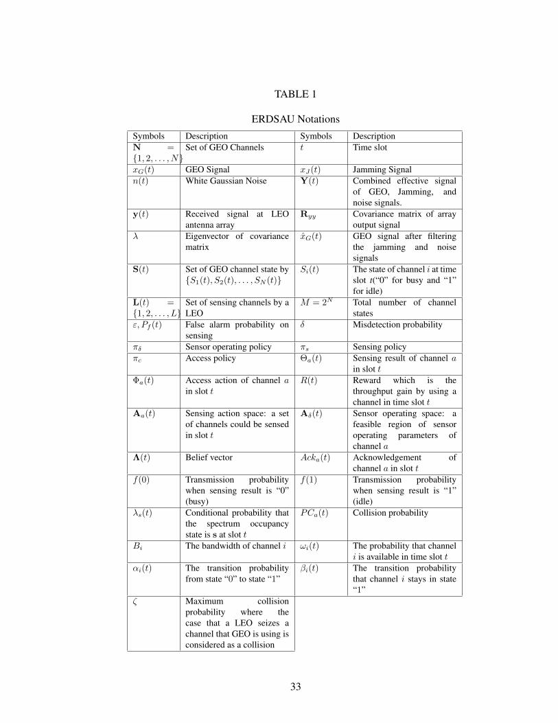
TABLE 1

ERDSAU NotationsSymbols Description Symbols DescriptionN ={1, 2, . . . , N}

Set of GEO Channels t Time slot

xG(t) GEO Signal xJ(t) Jamming Signaln(t) White Gaussian Noise Y(t) Combined effective signal

of GEO, Jamming, andnoise signals.

y(t) Received signal at LEOantenna array

Ryy Covariance matrix of arrayoutput signal

λ Eigenvector of covariancematrix

xG(t) GEO signal after filteringthe jamming and noisesignals

S(t) Set of GEO channel state by{S1(t), S2(t), . . . , SN (t)}

Si(t) The state of channel i at timeslot t(“0” for busy and “1”for idle)

L(t) ={1, 2, . . . , L}

Set of sensing channels by aLEO

M = 2N Total number of channelstates

ε, Pf (t) False alarm probability onsensing

δ Misdetection probability

πδ Sensor operating policy πs Sensing policyπc Access policy Θa(t) Sensing result of channel a

in slot tΦa(t) Access action of channel a

in slot tR(t) Reward which is the

throughput gain by using achannel in time slot t

Aa(t) Sensing action space: a setof channels could be sensedin slot t

Aδ(t) Sensor operating space: afeasible region of sensoroperating parameters ofchannel a

Λ(t) Belief vector Acka(t) Acknowledgement ofchannel a in slot t

f(0) Transmission probabilitywhen sensing result is “0”(busy)

f(1) Transmission probabilitywhen sensing result is “1”(idle)

λs(t) Conditional probability thatthe spectrum occupancystate is s at slot t

PCa(t) Collision probability

Bi The bandwidth of channel i ωi(t) The probability that channeli is available in time slot t

αi(t) The transition probabilityfrom state “0” to state “1”

βi(t) The transition probabilitythat channel i stays in state“1”

ζ Maximum collisionprobability where thecase that a LEO seizes achannel that GEO is using isconsidered as a collision

33

CHAPTER III

DISTRIBUTED GRAPH PARTITION AND EMBEDDING ON

LARGE-SCALE STREAMING NETWORK

This chapter presents a new graph embedding framework named as real-time and

distributed graph embedding (RTDGE), which can distributively embed large scale graph

in real-time. Specifically, we proposed an edge based graph partition to ensure balanced

partition. To handle streaming data input, a dynamic graph embedding approach was

provided without compromising the system efficiency and effectiveness. Then, we

adopted a heuristic global aggregation method to combine the locally embedded vector

spaces. Finally, our RTDGE algorithm was implemented and evaluated on the planform

which combined with Apache Kafka, Apache Zookeeper and Apache Storm. The

experimental results on various real-world data sets prove the effectiveness of our

algorithm.

A Mathematical Model

Let G(V,E) be a large graph, where V and E are respectively the vertex set and

edge set with |V | = N . Edge eij = (vi, vj) is defined as the directed link from vertex

vi to vj with associated weight ωij . The goal of graph embedding is to map the original

graph to a d-dimensional feature representation vector space (d << N ) while the original

34

similarities among vertices are maximally preserved. Accordingly, the optimization of

graph embedding can be mathematically written as:

O = min(s(~vi, ~vj)− s(vi, vj)), (10)

where ~vi and ~vj are the embedded vectors for vertex vi and vj , and s(·) is a pre-defined

similarity function.

In this paper, we adopt the similarity defined in LINE [27] and extend that to the

scenario of dynamic and distributed graph embedding. Specifically, the similarity is defined

in two aspects: (i) first-order proximity, and (ii) second-order proximity. The first-order

proximity is defined as the direct connection between two vertices. Since the first-order

proximity is insufficient to present the global structure of the graph, we also use the second-

order proximity, which is defined as the number of shared neighbors between two vertices.

For the graph shown in Fig.2, using the first-order proximity, the embedded vector ~v1 should

be closer to ~v2 than to ~v7 since vertices v1 and v2 are directly connected in the original graph.

Using the second-order proximity, ~v6 should be closer to ~v1 than to ~v5 because v6 and v1

have more shared neighbors in the original graph.

1 Problem Formulation

According to LINE [27], for the first-order proximity, the similarity between

vertices vi and vj (i.e., strength of their direct connection) is calculated as the following

empirical probability:

s(vi, vj) = p1(vi, vj) =ωijW, (11)

35

where W =∑

e∈E ωe is the total weights.

After graph embedding, the similarity between embedded vectors ~vi and ~vj is

calculated as the following probability:

s(~vi, ~vj) = p1(~vi, ~vj) =1

1 + exp(−~vTi · ~vj). (12)

Let d(·) denote the KL distance, and the optimization problem Eq.(10) becomes:

O1 = min d(p1(~vi, ~vj), p1(vi, vj)), (13)

where vectors ~vi and ~vj are the optimization variables.

Plug Eq.(11) and Eq.(12) into Eq.(13) and apply KL distance, then Eq.(13) can be

further written as:

O1 = min

− ∑(vi,vj)∈E

ωij log p1(~vi, ~vj)

. (14)

For the second-order proximity, the similarity between vertices vi and vj is

calculated as the following empirical probability:

p2(vj|vi) =ωijλi, (15)

where λi =∑

vj∈N(vi)ωij with N(vi) being vi’s neighborhood vertex set. Note that λi

represents the prestige of vertex vi in the network.

For the second-order proximity, according to LINE, each vertex in the original graph

also acts as a “context”. Let ~v′j denote the embedded vector when vj is treated as “context”,

the probability of ~v′j based on ~vi can be expressed as:

p2(vj|vi) =exp(~v′Tj · ~vi)|V |∑k=1

exp(~v′Tk · ~vi)

, (16)

36

The goal is to make the conditional distribution p2(·|vi) as close as possible to the empirical

distribution p2(·|vi). Therefore, based on the second-order proximity, the optimization

problem Eq.(10) becomes:

O2 = min∑vi∈V

λid(p2(·|vi), p2(·|vi)). (17)

Plug Eq.(15) and Eq.(16) into Eq.(17) and apply KL distance. Therefore, Eq.(17)

becomes:

O2 = min∑eij∈E

ωij log p2(vj|vi). (18)

B Real-time Distributed Graph Partition and Embedding

1 Graph Partition

To facilitate big data applications, we divide the incoming big data into many

clusters and then perform graph embedding distributively. The task of dividing a large

graph into several subgraphs is a classic problem called graph partition. Most existing

graph partition methods are based on vertex partition [20–22], which divide vertices into

un-overlapped subgraphs. However, the main drawback of vertex based partitions is that

they cannot guarantee balanced graph partitions due to the uncertainty of the degree of

each vertex. In this paper, we propose a new edge based graph partition method with the

following features:

• It avoids unequal graph partition. In real-time streaming applications, an edge is the

basic input unit for graph partition and embedding. Meanwhile, the computational

37

Bbg v1,v2,v3,v4,v6

Bgy v3,v4,v5,v6

Bby v3,v4,v6,v7,v8

Bbgy v3,v4,v6

v1

v2

v3

v4

v5

v6

v7v8

Figure 2: Edge Partition.

complexity of graph embedding depends on the number of edges (rather than

vertices) in the subgraph. As a result, our edge based method simplifies the partition

process and balances the complexity of the distributed machinery.

• The similarities among vertices (prior to partition) are maximally preserved after

graph partition.

• It completely eliminates communication overhead among clusters during the

partition process.

For a given graph G = (V,E), all the edges are divided into K different subgraphs

Gk = (Vk, Ek) without overlapping, i.e.,

E = ∪Kk=1Ek ∀i, j : i 6= j ⇒ Ei ∩ Ej = ∅, (19)

where K is the pre-set total number of subgraphs. Note that adjacent subgraphs usually

have overlapped vertices. We denote Bij = {vk|vk ∈ Vi ∩ Vj} as the overlapped vertex set

between subgraphGi andGj , where Vi and Vj are the vertex sets ofGi andGj respectively.

Fig. 2 shows three subgraphs Gb, Gg, Gy, whose edges are colored in blue, green

and yellow respectively. As we can see, v1 is connected by both blue and green edges so

38

that v1 belongs to both Gb and Gg (i.e., v1 ∈ Bbg). Accordingly, we have

Bbg = {v1, v2, v3, v4, v6}, Bby = {v3, v4, v6, v7, v8} and Bgy = {v3, v4, v5, v6}. Meanwhile,

vertices v3, v4 and v6 are shared by all three subgraphs.

In order to have a balanced graph partition, the size of each subgraph (i.e., the

number of edges) should be as close as possible to the average size of |E|/K. Therefore,

we use the standard deviation of the subgraph size to measure the balance of graph partition:

std =

√∑Kk=1( |Ek|

|E|/K − 1)2

K. (20)

For subgraph Gk, let Z(k),Y (k),∈ R|Vk|×d be the d-dimensional embedded vector

sets by subgraph embedding and global embedding, respectively. The objective function

for graph partition optimization is:

min∑||Z(k) − Y (k)||2. (21)

Furthermore, the communication cost among the whole partitions also need to be

considered. In order to have a effective performance on the following aggregation process,

the communication cost should be as small as possible which is defined as the number of

overlapping vertices:

min∑i

∑j

|Bij|, (22)

where Bij is the overlapping vertex set between two subgraphs Gi and Gj , for ∀i,∀j ∈

[1, K], i 6= j as we discussed above.

In [50], author provides an ideally simple solution that: to compute K partitions,

K edges are chosen at random and each partition grows around those edges. Then, all

39

partitions take control of the edges that are neighbors of those already in control and are

not taken by other partitions. All partitions will incrementally get larger and larger until

all edges have been taken. However, this method is not practical in real-world cases, since

the starting position may influence the size of the partitions. For instance, a partition that

starts from the center of the graph will have more space to expand than a partition that starts

from the border and/or very close to another partition. Additionally, thus graph partition

problem is a NP-hard problem in general [20, 51]. To overcome this issuer, we propose our

greedy one-pass edge partition algorithm consumes the subgraphs in a streaming fashion

which means requiring only a single pass. Besides, in order to preserve the original graph

similarity for each subgraph, we also consider balanced weights in partitions due to the

above analysis that the empirical probability is effected by the total weights. It proceeds as

followings:

• Initially, all K subgraphs are open to accept new edges. A subgraph will be

considered closed if its capacity (maximally number of edges allowed) is reached.

• An incoming edge e = (u, v) will be assigned to the subgraph who has the minimum

weight among all subgraphs containing vertex u or v, where the weight of subgraph

Gk is given by∑

e(u,v)∈Ekωuv.

• In order to balance the number of edges |Ek| in each subgraph (k = 1, 2...K), we

set a given threshold te, if max (|Ek|) − min (|Ek|) ≥ te, the next incoming edge

with the minimum weight over time (from the beginning to the current state) will be

assigned to the subgraph with min (|Ek|).

40

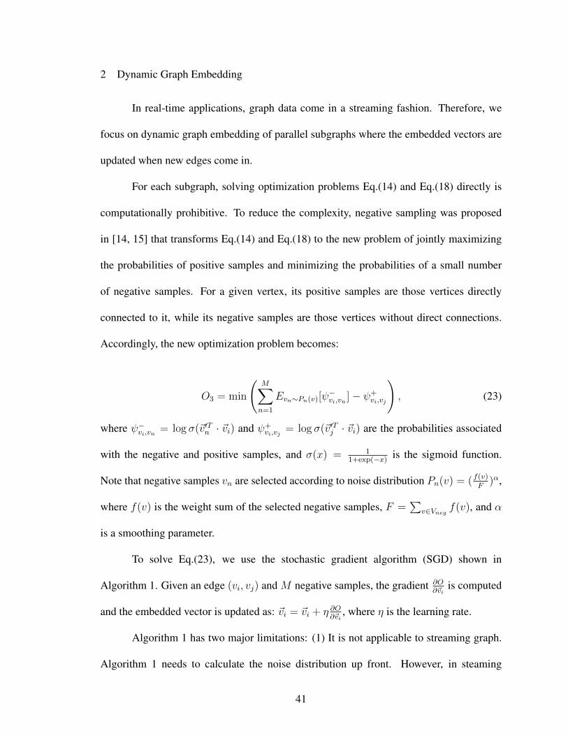
2 Dynamic Graph Embedding

In real-time applications, graph data come in a streaming fashion. Therefore, we

focus on dynamic graph embedding of parallel subgraphs where the embedded vectors are

updated when new edges come in.

For each subgraph, solving optimization problems Eq.(14) and Eq.(18) directly is

computationally prohibitive. To reduce the complexity, negative sampling was proposed

in [14, 15] that transforms Eq.(14) and Eq.(18) to the new problem of jointly maximizing

the probabilities of positive samples and minimizing the probabilities of a small number

of negative samples. For a given vertex, its positive samples are those vertices directly

connected to it, while its negative samples are those vertices without direct connections.

Accordingly, the new optimization problem becomes:

O3 = min

(M∑n=1

Evn∼Pn(v)[ψ−vi,vn

]− ψ+vi,vj

), (23)

where ψ−vi,vn = log σ(~v′Tn · ~vi) and ψ+vi,vj

= log σ(~v′Tj · ~vi) are the probabilities associated

with the negative and positive samples, and σ(x) = 11+exp(−x)

is the sigmoid function.

Note that negative samples vn are selected according to noise distribution Pn(v) = (f(v)F

)α,

where f(v) is the weight sum of the selected negative samples, F =∑

v∈Vnegf(v), and α

is a smoothing parameter.

To solve Eq.(23), we use the stochastic gradient algorithm (SGD) shown in

Algorithm 1. Given an edge (vi, vj) and M negative samples, the gradient ∂O∂~vi

is computed

and the embedded vector is updated as: ~vi = ~vi + η ∂O∂~vi

, where η is the learning rate.

Algorithm 1 has two major limitations: (1) It is not applicable to streaming graph.

Algorithm 1 needs to calculate the noise distribution up front. However, in steaming

41

Algorithm 1Input: enew = (u, v), G′ = (V ′, E ′), negativesample set |Vneg|Initialization: f(v)← 0 for all v

1: for i = 1, 2, . . . , n do2: f(v)← f(v) + ωenew

3: F =∑

v∈Vnegf(v)

4: Pn ← f(v)3/4

F 3/4

5: for v ∈ enew6: draw M negative samples from Pn

7: use SGD to update ~v

8: end for9: end for

applications, the graph data is only partially available at any given time. (2) The

complexity of Algorithm 1 is too high for large scale data sets. Calculating the noise

distribution requires a search over the entire vertex set, which will exhaust the computing

power and memory of distributed workers. To overcome these two issues, we propose

Algorithm 2 to only keep track of the top-L frequent vertices in calculating the noise

distribution, based on partially observed graph. In this way, we can handle streaming big

data input with significantly reduced complexity.

Remark 1: Algorithm 2 targets for streaming applications, where the top-L frequent

vertices and the noise distribution are based on current partial graph and they are constantly

updated as more data come in.

Remark 2: The negative sampling method is implemented by a vertex array known

as negative table T , where the number of copies of vertex v appended into the table is

proportional to Pn(v). Then, a negative sample is generated by uniformly selecting an

element from the negative table. In Algorithm 2, τ is the maximum size of the negative

42

Algorithm 2Initialization: f(v)← 0 for all v

z ← 0

1: for i = 1, 2, . . . do2: f(v)← f(v) + ωenew

3: dif = f(v)3/4 − (f(v)− ωenew)3/4

4: z ← z + dif

5: if |T | < τ

6: add dif copies of v to the negative table

7: else8: for j = 1, 2, . . . , |T |9: T [j]← vwith probability dif

z

10: end for11: end if12: end for

table. When |T | < τ , dif copies of vertex v can be added directly into the table. When

|T | = τ , element T [j] will be replaced by vertex v with probability difz

.

Remark 3: The complexities of Algorithm 1 and 2 are respectively O(|E|) and

O(τ), where τ << |E|.

3 Heuristic Global Aggregation

The last step of RTDGE is global aggregation of the distributively embedded

subgraphs. The basic idea of our unsupervised global aggregation is to find a feasible

global vector space which mapping from multiple local embedding sub-spaces by utilizing

the overlapped vertex set B.

Assume vertex vm belongs to multiple subgraphs, e.g., Gi and Gj indicated by

vm ∈ Bij; Z(i) = F (Gi) and Z(j) = F (Gj) are the local embedded vector spaces of Gi

43

and Gj respectively. As a result, the local embedded vectors of vm in subgraph Gi and Gj

can be expressed as z(i)m and z

(j)m respectively. If there exists a mapping function

h(z

(i)m , z

(j)m

)−→ym for the overlapped vertex vm, we can use this function to map the

entire subspace Z(i) and Z(j) into a global vector space Y :

h(Z(i),Z(j)

)h(z

(i)m ,z

(j)m )−→ Y . (24)

We design a low complexity unsupervised global aggregation algorithm by applying

the linear transformation method. The designed algorithm which is simple but effective

includes two processes: (1) normalization and (2) combination. Specifically, we first find

the overlapped vertex set Ball = V1 ∩ V2 ∩ . . . ∩ VK among all subgraphs. Then, for each

vertex vm ∈ Ball, we normalize its local embedded vector zim = [zim(1), zim(2), . . . , zim(d)]

in every cluster i as:

z(i)′

m = [zim(1)− eim

σ(i)m

,zim(2)− eim

σ(i)m

, . . . ,zim(d)− eim

σ(i)m

], (25)

where eim =∑zim(1)+zim(2)+···+zim(d)

dis the mean value of zim and σ(i)

m

2is the variance.

After normalization process, the combination process is conducted to find/form the

global space by combining the normalized embedded vectors in different local clusters

of each overlapped vertex. While various combination method can be applied, we adopt

the average operator. By using Eq.(25), the average of the normalized vectors of vertex

vm is calculated as: z′m =

∑Ki=1 z

(i)′m

K. Therefore, the mapping function for vertex vm can

be expressed as: zim = hm

(z

(i)m , z

(j)m

). Then, the global standard embedded vector is

calculated as:

z(all) =

∑m∈Ball

z′

m

|Ball|. (26)

44

TABLE 2

Data sets used for experiments in Section IV.

Name Edges # Vertices #

AstroPH 196,972 17,903USRoad 3,083,796 2,541,898

Les Miserables 254 77BlogCatalog 333,983 10,312Wikipedia 184,812 4,777YouTube 4,945,382 1,138,499

Furthermore, the local graph embedded vector space Z(i) can be mapped to a partial

global vector space y′i as:

y′

i = Z(i) − dist(i), (27)

where dist(i) =

∑vm∈Vi∩Ball

(z(i)m − z(all)

)|Vi∩Ball|

∀vm ∈ Vi ∩B(all).

Finally, the global feature representation Y can be produced as:

Y =[y′1,y

′2, . . . ,y

′K

].

C Experiments

1 System Setup

In order to implement our RTDGE algorithm and evaluate its real-world

performance, we develop a real-time distributed graph embedding platform based on

Apache Kafka and Apache Storm. The system consists of three servers: each server has

8GB memory, quad-core Intel Xeon CPU and 500GB disk space. The connection among

servers are constructed by Apache Zookeeper. Unlike GraphX that is only built upon

Apache Spark, in our platform the streaming data are retrieved by Apache Kafka and

45

Figure 3: Subgraph Size Stand Deviation Evaluation.

Figure 4: Maximum Subgraph Size.

distributed into multiple brokers according to our edge partition algorithm in Section III.

A typical Apache Kafka consists of a producer and a consumer. Multiple producers and

consumers can publish and retrieve data at the same time. A data message is defined as a

topic, which can be divided into multiple partitions. One or more partitions can be stored

in each broker. The data in each broker can be consumed by one or multiple Apache

Storm clusters including one Apache Storm Nimbus and multiple Apache Storm

Supervisors. The data sets we used for experiments are summarized in TABLE 2.

46

2 Graph Partition

In Fig. 3 and Fig. 4, we compare the performance of our approach with two other

methods. Distributed funding-based edge partitioning (DFEP) is an edge partition

algorithm based on the concept that every vertex has certain amount of money to buy

assigned edges, and DFEPC is another version of DFEP with different parameters. In [50],

the authors show that DFEP and DFEPC outperform METIS using the following two data

sets: (1) AstroPH [52] is a weighted network of co-authorships among scientists posting

preprints on High-Energy Theory E-Print Archive between Jan 1, 1995 and December 31,

1999. It has 17, 903 vertices and 196, 972 edges. (2) USRoad is a road network in

Pennsylvania where nodes represent the intersections and endpoints while edges represent

roads. The network has 2, 541, 898 nodes and 3, 083, 796 edges. The metrics we used to

evaluate the performance are: (i) Standard deviation of subgraph size by Eq.(20); (ii) The

size of the largest subgraph normalized by the average subgraph size. From Fig. 3 and

(a) (b) (c)

Figure 5: Original Les Miserables network at (a) T = ti, (b) T = tj , (c) T = tk.

Fig. 4, we can see that both the variance of the subgraph size and the size of the largest

subgraph increase with the number of subgraphs for all partition methods. Apparently, our

algorithm outperforms others with a large margin in all cases. In particular, when K is

increased from 10 to 100, our algorithm is able to keep the standard deviation close to zero

47

and the size of the largest subgraph is very close to one (i.e., the average subgraph size).

3 Dynamic Graph Embedding

Since our dynamic graph embedding is designed for streaming data input, it is

capable of revealing the evolution of network structure over time. In this section, we use

the famous novel Les Miserables by Victor Hugo as a case study to illustrate the

effectiveness of our dynamic graph embedding. The Les Miserables network contains

co-appearances of 77 characters. In graph representation, a node represents a character

and an edge means that these two characters appear in the same chapter of the book. There

are 254 edges in this network. The weight of each link indicates how often such a

co-appearance occurs. We embed the Les Miserable network into a 3 dimensional vector

space and monitor the embedded results at three different time instances:

• T = ti, the network has ten characters.

• T = tj , the network has eleven characters (the main character Valjean appears).

• T = tk, the network has sixteen characters.

When T = ti, tj , tk, Fig. 5 shows the original Les Misrable graph. Fig. 6 consists of

the visualizations of the embedded results. As we can see in Fig. 12a, the embedded nodes

are clustered into three different groups. It turns out that the isolated red node (Node 0) is

character Myriel who plays an important role at the beginning. Myriel is also shown in Fig.

5a as the center node with an unique connection pattern. Therefore, it is reasonable to be

isolated in the embedded space. Furthermore, the green nodes are Node 2 (MlleBaptistine)

and Node 3 (MmeMaglorie), who have the same connection pattern (i.e., connected with

48

each other and only linked with Node 0) distinguished from others. As a result, they are

located in the same position after graph embedding. We also see that the remaining black

nodes are close since they are similar by the first-order proximity.

When T = tj , Fig. 12b illustrates the embedded results. A new Node 11 (Valjean) is

embedded closely to Node 2 and Node 3. In Fig. 5b, Node 11 is more similar to Node 2 and

3 by the first-order proximity. However, by the second-order proximity, Node 11 clearly

has different connection pattern from Node 2 or 3, as shown by their distances in Fig. 12b.

On the other hand, the black nodes are almost overlapped because their connection patterns

are very similar.

When T = tk, the graph embedding results under first-order proximity and second-

order proximity are shown in Fig. 6c and 6c, respectively. In Fig. 6c, there are two isolated

nodes, Node 0 (Myriel, colored in red) and Node 11 (Valjean, colored in cyan). Besides,

there are two node clusters: one contains black stars which are existing characters; the other

cluster contains blue circles which are new characters. According to our previous analysis,

nodes in the same cluster should share similar connection pattern. As shown in Fig. 5c,

new nodes are only connected with Node 11 (Valjean).

4 Multi-label Classification

In multi-label classification setting, each node is assigned one or more labels from

a finite set L. During the training phase, we observe a certain fraction of nodes with their

labels. The objective is to predict the labels of the remaining nodes, which is challenging

when L is large. In our experiments, we evaluate the performance of our RTDGE by

comparing it with the following algorithms:

49

(a) 3D Graph embedding before Valjean appears (T = ti)

(b) 3D Graph embedding when Valjean appears (T = tj)

(c) 3D Graph embedding after Valjean appears (T = tk)

Figure 6: Dynamic graph embedding results.

50

TABLE 3

Multi-label classification results of BlogCatalog.

Metric Algorithm 10% 20% 30% 40% 50% 60% 70% 80% 90%

Macro-F1 SpectralClustering 3.01 3.21 3.49 4.01 4.22 4.50 4.81 5.01 5.11DeepWalk 5.03 7.53 9.03 10.03 11.03 11.33 11.63 11.93 12.63LINE1st 13.65 13.69 13.77 13.57 14.06 13.51 13.31 14.69 13.27LINE2nd 13.88 13.75 13.54 13.88 13.71 13.37 12.91 13.18 13.08

RTDGE1st 14.01 14.08 14.13 14.19 14.25 14.39 14.61 14.72 14.76RTDGE2nd 13.79 13.81 13.71 13.92 13.78 14.02 13.96 14.13 13.95

Micro-F1 SpectralClustering 16.15 17.51 17.91 18.11 18.99 19.76 20.87 21.03 22.19DeepWalk 16.53 18.73 20.13 20.83 21.53 21.83 22.03 22.03 22.5300LINE1st 22.04 18.34 23.12 21.90 23.16 22.95 24.12 24.34 24.43LINE2nd 15.25 12.97 13.94 14.22 14.65 14.04 13.18 15.01 15.29

RTDGE1st 24.57 24.77 24.76 24.85 24.24 24.71 24.21 24.29 24.66RTDGE2nd 24.21 24.25 24.10 24.44 24.23 24.58 24.49 24.76 24.29

• Spectral clustering [53] is a matrix factorization approach where the top d

eigenvectors of the normalized Laplacian matrix are used as nodes’ feature vector

representations.

• DeepWalk [16] is a classic graph embedding approach, where random walks are

generated from each vertex to obtain the contextual information of the network.

• LINE [27] contains an edge sampling method that improves the computational

efficiency over the traditional SGD method. It has two proximities: LINE1st and

LINE2nd.

BlogCatalog: We first use BlogCatalog dataset as our input graph. It is a network of

social relationships of the bloggers publicly available on BlogCatalog website

(http://blogcatalog.com). There are 10, 312 users and 333, 983 edges in the network. Each

edge represents the friendship between two users. To accomplish the goal of classification,

the embedded vectors are input to a one-vs-all logistic regression classifier with L2

51

regularization. The well-known Macro-F1 and Micro-F1 scores are used as the

performance metric.

TABLE 3 shows the MicroF1 and Macro-F1 scores with different percentage of

train data, which is used to train the L2 logistic regression model with λ = 1. The results

are averaged over 10 different trials. Apparently, our algorithm achieves higher Micro-F1

scores than other methods, especially under the second-order proximity. This is because:

(1) We use adaptive N -Gram Negative method instead of the fixed N-Gram Negative (i.e.,

N = 5) method used by LINE. (2) Unlike LINE which uses negative samples from

neighboring nodes, we carefully consider each vertex’s connection pattern to avoid using

neighboring nodes as negative samples and guarantee all negative samples are selected

according to the noise distribution. For the Macro-F1 score, our algorithm is able to

achieve almost the same performance as LINE.

TABLE 4

Multi-label classification results of Wikipedia.

Metric Algorithm 10% 20% 30% 40% 50% 60% 70% 80% 90%

Macro-F1 SpectralClustering 4.01 4.02 4.03 4.11 4.51 4.69 4.78 4.91 5.01DeepWalk 8.91 10.02 11.09 12.14 12.51 13.71 15.88 17.09 22.46LINE1st 47.05 47.18 46.81 46.93 46.68 46.98 46.98 46.24 47.27LINE2nd 47.06 47.02 46.99 46.83 464.57 47.09 47.09 46.52 46.79

RTDGE1st 47.05 47.18 46.89 46.95 47.4 47.08 46.96 46.75 47.51RTDGE2nd 47.12 47.04 47.16 47.28 47.08 47.32 47.35 47.23 47.15

Micro-F1 SpectralClustering 41.01 40.50 40.31 40.22 40.28 40.27 40.17 40.06 38.51DeepWalk 46.49 48.27 51.12 52.17 52.35 52.25 52.26 52.25 52.24LINE1st 63.99 64.12 63.77 63.89 63.65 63.92 63.89 63.23 64.17LINE2nd 28.73 26.71 22.31 23.93 23.49 30.96 26.19 32.94 43.23

RTDGE1st 63.92 63.95 63.79 63.89 64.31 64.02 63.75 63.71 64.38RTDGE2nd 64.06 63.96 63.94 63.79 63.55 64.03 64.02 64.14 63.74

Wikipedia: This is a co-occurrence network of words appearing in the first million bytes of

Wikipedia. There are 40 different labels which represent the Part-of-Speech tags by using

52

the Standard POS-Tagger. The network contains 4, 777 nodes and 184, 812 edges.

TABLE 4 illustrates the multi-label classification results. For the Macro-F1 score

metric, our algorithm outperforms LINE and achieves the highest score at the end point.

For the first-order proximity, our Micro-F1 score has 60% gain over the spectral clustering

algorithm. For the second-order proximity, our Micro-F1 score has 55% gain over the

spectral clustering method. Compared to LINE, RTDGE also performs better under both

first-order and second-order proximity.

TABLE 5

Multi-label classification results of YouTube.

Metric Algorithm 1% 2% 3% 4% 5% 6% 7% 8% 9% 10%

Micro-F1 SpectralClustering 24.97 26.48 27.25 27.87 28.31 28.68 29.01 29.21 29.36 29.63DeepWalk 39.68 41.78 42.78 43.55 43.96 44.31 44.61 44.89 45.06 45.23

LINE 40.20 42.70 43.94 44.71 45.19 45.55 45.87 46.15 46.33 46.43RTDGE10 40.68 43.58 46.39 47.63 48.87 49.70 50.64 50.78 50.86 50.74RTDGE30 44.32 44.51 44.53 44.66 44.96 45.27 5.31 45.84 48.20 52.03RTDGE50 42.22 43.35 44.07 44.48 44.71 44.90 45.14 45.41 45.53 45.54

Macro-F1 SpectralClustering 11.01 13.55 14.93 15.90 16.45 16.93 17.38 17.64 17.80 18.09DeepWalk 28.39 30.96 32.28 33.43 33.92 34.32 34.83 35.27 35.54 35.86

LINE 29.85 31.93 33.96 35.46 36.25 36.90 37.48 38.10 38.46 38.82RTDGE10 37.8800 38.0300 38.1000 38.1400 38.1600 38.2100 38.3100 38.4900 38.8000 39.2500RTDGE30 38.1094 38.1476 38.1501 38.1755 38.2358 38.2962 38.3051 38.4099 38.8742 39.6300RTDGE50 37.2082 37.2273 37.2297 37.3355 37.3498 37.4614 37.4800 37.5334 37.7235 38.4010

YouTube: YouTube network is much sparser than other social networks. The dataset has

4,945,382 edges and 1,138,499 nodes. The results are summarized in TABLE 5. We divide

the original large-scale graph into 10, 30 and 50 partitions, respectively. We can see that the

classification accuracy remains stable with different number of partitions. For the Micro-F1

score, our algorithm has nearly 20% and 10% gains over DeepWalk and LINE, respectively.

For the Macro-F1 score, our algorithm also outperforms other approaches.

53

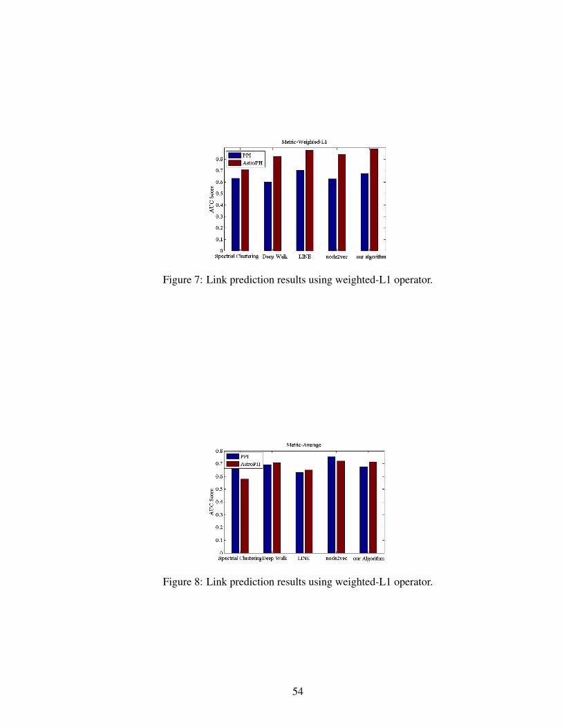
Figure 7: Link prediction results using weighted-L1 operator.

Figure 8: Link prediction results using weighted-L1 operator.

54

5 Link Prediction

In social network, link prediction aims to predict the potential relations (i.e., missing

edges) among existing nodes when only fractional edges are known. The positive samples

are generated by removing 50% edges randomly, while the graph remains connected. To

obtain negative samples, the same number of unconnected node pairs from the graph are

selected. The following datasets are used for link prediction:

• Protein-Protein Interactions (PPI) network contains 19,706 nodes and 390,633 edges,

where each node represents one type of proteins and each edge is the biological

interaction between the pair of proteins.

• AstroPH is a weighted network of co-authorships among scientists posting preprints

on High-Energy Theory EPrint Archive between Jan 1, 1995 and December 31, 1999.

It has 17,903 vertices and 196,972 edges.

We follow the same edge feature learning settings as node2vec. Assume embedded vectors

~vi, ~vj are the feature representations of node vi and vj , the edge feature g(vi, vj) between

node vi and vj can be represented as: (1) Average operator: g(vi, vj) =~vi+~vj

2; (2) Weighted-

L1 operator: g(vi, vj) = |~vi − ~vj|. By applying the logistic regression, the results are

shown in Fig. 7 and Fig. 8. We can see that our algorithm has the best performance for

AstroPH dataset. For PPI dataset, our RTDGE achieves similar AUC score as LINE with

significantly reduced runtime.

TABLE 6 shows the runtime of all algorithms. Clearly, our RTDGE is the fastest

algorithm. Specifically, we implement all algorithms in Java on a single machine with

32GB memory, AMD Threadripper 16-core CPU and 1TB SSD. Remarkably, our RTDGE

55

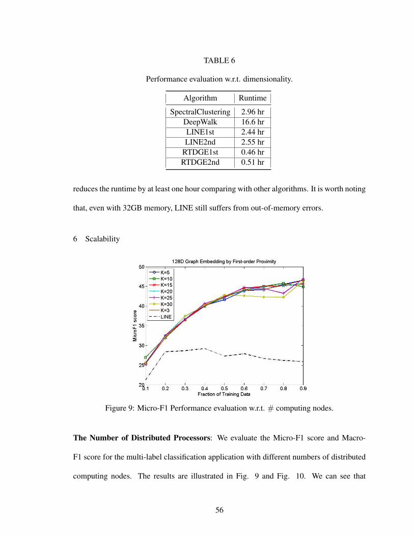
TABLE 6

Performance evaluation w.r.t. dimensionality.

Algorithm Runtime

SpectralClustering 2.96 hrDeepWalk 16.6 hrLINE1st 2.44 hrLINE2nd 2.55 hr

RTDGE1st 0.46 hrRTDGE2nd 0.51 hr

reduces the runtime by at least one hour comparing with other algorithms. It is worth noting

that, even with 32GB memory, LINE still suffers from out-of-memory errors.

6 Scalability

Figure 9: Micro-F1 Performance evaluation w.r.t. # computing nodes.

The Number of Distributed Processors: We evaluate the Micro-F1 score and Macro-

F1 score for the multi-label classification application with different numbers of distributed

computing nodes. The results are illustrated in Fig. 9 and Fig. 10. We can see that

56

Figure 10: Macro-F1 Performance evaluation w.r.t. # computing nodes.

our RTDGE is able to hold the performance when the number of distributed processors

increases.

Dimensionality: To study the effect of dimensionality on classification, we embed the

original Wikipedia network (i.e., R4777×4777) into five different dimensional spaces:

R4777×3, R4777×16, R4777×64, R4777×128 and R4777×256. The results are illustrated in TABLE

7. We can see that the performance of RTDGE increases with the dimensionality of the

embedded space, and 256D embedding achieve the highest scores. On the other hand, 3-D

embedding is able to achieve a decent performance with significantly reduced

computation cost.

Speed Performance: Fig. 11 shows the speed up versus the number of partitions. As

expected, the speed up ratio increases with the number of partitions (linear when K is less

than 10).

57

TABLE 7

Performance evaluation w.r.t. dimensionality.

Metric Dimensionality 10% 20% 30% 40% 50% 60% 70% 80% 90%

Micro-F1 3D 45.70 46.64 46.74 46.91 46.96 47.05 47.09 47.12 47.2316D 46.57 46.79 46.83 46.90 46.98 47.06 47.12 47.34 47.3664D 46.69 46.83 46.90 46.91 46.99 47.08 47.17 47.40 47.51

128D 46.75 46.84 46.90 46.96 47.03 47.10 47.18 47.41 47.74256D 46.78 46.89 46.95 46.94 47.05 47.19 47.38 47.56 47.75

Macro-F1 3D 62.72 63.59 63.70 63.85 63.91 63.95 64.02 64.05 64.1516D 63.65 63.75 63.79 63.86 63.92 63.99 64.03 64.26 64.2764D 63.71 63.75 63.79 63.86 63.93 64.01 64.05 64.31 64.38

128D 63.54 63.79 63.84 63.88 63.94 64.04 64.11 64.32 64.61256D 63.74 63.84 63.85 63.89 63.97 64.12 64.30 64.46 64.63

0 5 10 15 20 25 300

5

10

15

20

25

30

Number of Partitions

Spee

d up

Rat

io

Figure 11: Speed up w.r.t Number of Partitions

58

CHAPTER IV

REAL-TIME DEEP ANALYSIS OF TWITTER NETWORK

In previous chapter, the distributed graph embedding platform and the first

algorithm RTDGE have been introduced. A real-world application: Twitter network

analysis is demonstrated in this chapter. The Twitter data including posted twitters,

following and follower lists of Twitter accounts can be retrieved in real-time. A

comprehensive graph is generated to describe the relationships among Twitter users by

combining those multiple data types from Twitter. Then, the proposed graph partitioning

and embedding algorithm RTDGE is adopted to learn the representations of Twitter users

in lower dimensional vector space. Furthermore, real-world tasks are applied including

similar node detection, cluster and community classification and visualization.

Nowadays, millions people share their thoughts, stay in touch with friends, meet

new people and make work-related connections on social medias. Such social networks

whose nodes represent people or other entities embedded in the social context, and whose

edges represent interactions, collaborations or influences between entities are highly

dynamic objects. They grow and change quickly over time through the addition/deletion

of edges, signifying the appearance of new interactions in the underlying social structure.

Twitter network is one of the fastest growing social media network. It becomes a source of

varied kind of information, and any new type of data can be harvested from it. People

59

freely comment, discuss, compliment, argue and complain over topics they interested in,

no matter where they come from, what religious belief they hold, rich or poor. Studies

([54–57]) have well recognized that those contents and interactions generated by Twitter

users should be utilized for many applications. Collecting such rich and essential

information and understanding the deep relationships of social interactions among users

by which they evolves are fundamental questions that are still not well studied. Therefore,

this forms the motivation for our work.

Most of Twitter analysis approaches only focus on the semantic analysis of tweets,

i.e., instant messages created and spread by Twitter users or one simple relationship

between pair of Twitter users, i.e., if they are friends in Twitter network. Semantic

analysis of tweets is capable of extracting useful information from tweets, but the overall

or general tendency towards topics and structural roles of people can rarely be captured

due to their presentations in the diverse scenarios. For example, people read news about

elections, it is expected to get an overview about the support and opposition for

presidential candidates from Twitter. Fans of sports are fascinated about what is going on

on the pitch and the reactions from other people. In all of these scenarios, a

comprehensive analysis of the topics and interactions is needed. Twitter topic plays an

important role in such scenarios. People are connected to community-driven content

which has a certain topic, when they simply add a hash symbol # in the tweets, known as

topic of Twitter. It also benefits people to categorize and emphasize their options in their

tweets by using topics hashtags. The statistics shows that among 0.5 million randomly

selected tweets, around 35% of them have at lease one topic involved. In the Twitter

network, it also shows a great potential that people more likely tweet similar content and

60

follow each others, if they involve in same topics. Besides the relationship between user

and topic, it is also important to dig the connection between topics. In the experiment, the

probability for any two co-occurring topics to share same sentiment polarity is observed as

over 0.8055 [58].

However, none of existing approaches is capable of real-time extraction and

analysis of Twitter network. Furthermore, none of them jointly consider multiple

relationships among the Twitter users. As a result, we propose a unique information

extraction framework which is able to create a real-world complex graph from Twitter

network by maximally retrieving and combining structural information and social

interactions in real-time. The first implementation of the framework also is built with

consideration of three types of relationship graphs: (1) friend relationships among users;

(2) topic involving relationship between user and tweet; (3) Twitter topics co-occurrence

relationship.

Once the graph is ready, a powerful social network analysis tool is desired. The

traditional social network analysis approaches, e.g., PageRank [59], matrix factorization

[20, 23, 24], are unable to deal with large-scale networks, since they cannot avoid the

iterative matrix calculation or the computationally expensive eigen-decomposition. Recent

graph embedding approaches ([16, 25–27]) which are inspired by the advancement in

natural language processing embed each node of the graph into a lower dimensional space

while preserving the maximal structural information. The vectors is proved to facilitate

future applications such as link prediction or node classification. While graph embedding

is an intriguing idea, the existing algorithms have two major limitations: (1) None of them

can perform real-time graph embedding of streaming data. Specifically, current graph

61

embedding algorithms rely on prior knowledge of the entire graph and can only process

the data in a batched fashion, which is not applicable to real-time streaming applications.

(2) Most graph embedding algorithms are centralized, which is unable to handle big data.

Twitter generates massive graph data (e.g., interactions) in a very short period of time. In

this case, even a super computer could quickly deplete its resources (i.e., computation,

memory and storage). A distributed graph embedding platform based Apache storm has

been implemented which embeds the complex graph into a lower vector space.

Consequently, we propose a novel approach that generates a complex Twitter

network by combining such multiple relationships and interactions, and analyses the

similarity roles of Twitter users by using a distributed graph embedding method which is

able to facilitate any future social network based tasks. Our contributions can be

summarized as follows: (1) A framework is proposed to retrieve multi-types data by

applying Twitter API in real-time; (2) the first implementation of the framework is built

which dynamically generates a complex relation graph of certain Twitter users; (3)

distributed graph embedding algorithm is adopt to our platform for real-time graph

embedding.

A Real-time Complex Twitter Network Extraction

We propose a frame work in this section to jointly model the topological structure

and social activity information. We also provide an first comprehensive implementation of

our frame work. A complex Twitter network, denoted as G∗(V ∗, E∗), is created by

combining multiple fundamental graphs in real-time. The link and its strength in the

complex graph between any pair of users reflects the social activity information.

62

1 Fundamental Graphs

To accomplish the goal of real-time retrieving data from Twitter, Twitter API has

been developed. Twitter provides two different types of APIs: (i) RESTful API and (ii)

Streaming API. RESTful is used for historical Twitter data by setting up certain time

duration. On the contrary, Streaming API is able to monitor and retrieve data in real-time.

We successively implement our method by using both types of Twitter APIs. Additionally,

Twitter builds four libraries regarding to different coding languages, The library we use is

twitter4j. Instead of using text-based Twitter data which could be heterogeneous and

computationally expensive, we focus on combining multiple relationships from the

Twitter API. Specifically, in this paper, we extract three different fundamental graphs to

optimally represent the topological structure of the Twitter network and the social activity

information. Note that any other extracted graphs can be added to our frame work.

Definition 1 User Following Graph: G1 Intuitively, the following or followers in

Twitter defines the most basic relationship between pair of nodes. Assume G1 = (V1, E1)

denotes the user following graph in which each node ni ∈ G1 is a Twitter user and the edge

eij between users ni and nj represents if they followed each other or not.

Definition 2 Topic Involving Graph: G2 This graph describes the relation between

Twitter topics and Twitter users. There two two different types of nodes in this graph: (i)

Twitter user, e.g., realDonaldTrump and (ii) topics e.g., hashtag #PRStrong. Each edge

connects between a user node and a topic node, and it represents the number of times that

one users has tweeted about the topic.

Definition 3 Topic Co-occurrence Graph: G3 This graph is aiming to define the

relationship among topics. Hence, the graph consists of topic nodes only. An edge exists,

63

if two different topics are appeared in same tweet. For instance, the Twitter user

realDonaldTrump uses #NYCStrong#USA in one of his tweets. Then, there is an edge

between #NYCStrong and #USA. The weight of an edge is the number of times of the

co-occurrence of two topics.

2 Complex Graph Generation

We now introduce how to generate a complex graph which represents the

topological structure and social activity information from Twitter network. Assume the

complex graph is generated by:

G∗(V ∗, E∗) = gen(G1, G2, . . . , GL|policy) (28)

where G1, . . . , GL is the number of L fundamental graphs can be retrieved by Twitter API,

and the policy is the designed generation rule.

Definition 4 policy (Complex Graph Generation Rule) It defines how to combine

multiple graphs into one complex graph. More specifically, the policy is given to find

the feasible mappings from each fundamental graph to the complex graph. Therefore, the

intensity, i.e., ω∗ij of the relationship between pair of nodes, i.e., e∗ij in the complex graph

G∗ can be computed once a policy is defined.

In this paper, we build the first implementation of this frame by using a simple linear

combination method, such that the complex graph is given by:

G∗ = λ1G1 + λ2G2 + . . .+ λLGL (29)

where λ1 + λ2 + . . . + λL = 1. We consider the three fundamental graphs discussed in

64

Section 1. Each of simple graph has partial effort to impact the relationship of nodes, such

as if two users join more common topics, or if the topic which they involved are strongly

related, then they should be closer.

The first element in Eq. 29 is aiming to reflect the user following relationship by

multiplying the weight coefficient parameter λ1 with the edge e(1)ij in graphG1, i.e., the user

following graph. Note that, e(l)ij to indicate that if there is an edge existing between node i

and node j in fundamental graphGl or not. More over, the weight of the edge is denoted as:

ω(l)ij . When ω(l)

ij > 0, the edge e(1)ij exists in graph Gl. Furthermore, the second item in Eq.

29 is to accomplish the goal of compromising topic involving relationship between user i

and user j, we assume Topici indicates the topic set that user i has involved, similarly, we

have Topicj to be the topic set for user j. So that, if both user i and user j join the topic h

(i.e., they have tweeted at least one tweet with regarding to topic h), we are able to find the

corresponding edges e(2)ih and e(2)

jh in fundamental graph G2, i.e., topic involving graph, and

the corresponding weights are ω(2)ih and ω(2)

jh , respectively. It is reasonable to assume that

if two users tweet more frequently with respect to a same topic, their Twitter activities are

more in common. Noticing that we do not try to distinguish the users attitude to the topic

(i.e., positive or negative) yet, we only focus on the degree of the involvement between

user and the topic. Therefore, the compromised intensity of the relationship in terms of

topic h between user i and user j can be expressed as: λ2 ∗ (ω(2)ih + ω

(2)jh ). Consequentially,

for all shared topic h, i.e., ∀h ∈ Topici ∩ Topicj , we use the sum of the weights and

times with weight coefficient λ2 to represent the impact of the relationship between i and

j from graph G2. The last but not least, we consider the relationship from G3 by checking

the relationships among the uncommon topics. For instance, topic k ∈ Topici and topic

65

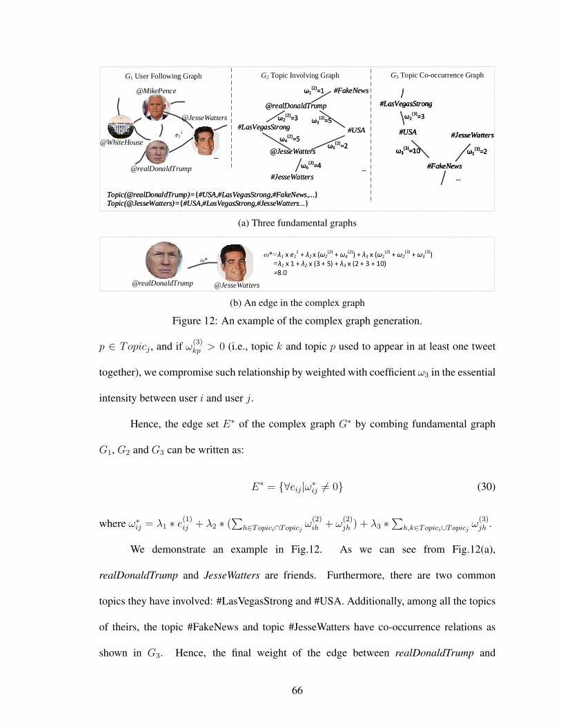
@realDonaldTrump

@MikePence

@JesseWatters

@WhiteHouse

ω2(2)=3

#LasVegasStrong

@realDonaldTrump

@JesseWatters

#USA

#FakeNews

#JesseWatters

ω3(2)=5

ω4(2)=5

ω5(2)=2

ω6(2)=4

ω1(2)=1

ω2(2)=3

#LasVegasStrong

@realDonaldTrump

@JesseWatters

#USA

#FakeNews

#JesseWatters

ω3(2)=5

ω4(2)=5

ω5(2)=2

ω6(2)=4

ω1(2)=1

G1 User Following Graph G2 Topic Involving Graph G3 Topic Co-occurrence Graph

@realDonaldTrump

ω*ω*=λ1 x e1

1 + λ2 x (ω2(2) + ω4

(2)) + λ3 x (ω1(3) + ω2

(3) + ω3(3))

=λ1 x 1 + λ2 x (3 + 5) + λ3 x (2 + 3 + 10) =8.0

@JesseWatters

...

...

e11

...

#LasVegasStrong

#USA

#FakeNews

#JesseWatters

ω3(3)=10 ω1

(3)=2

#LasVegasStrong

#USA

#FakeNews

#JesseWatters

ω3(3)=10 ω1

(3)=2

ω2(3)=3

#LasVegasStrong

#USA

#FakeNews

#JesseWatters

ω3(3)=10 ω1

(3)=2

ω2(3)=3

Topic(@realDonaldTrump)={#USA,#LasVegasStrong,#FakeNews,...}

Topic(@JesseWatters)={#USA,#LasVegasStrong,#JesseWatters...}



(a) Three fundamental graphs

@realDonaldTrump

@MikePence

@JesseWatters

@WhiteHouse

ω2(2)=3

#LasVegasStrong

@realDonaldTrump

@JesseWatters

#USA

#FakeNews

#JesseWatters

ω3(2)=5

ω4(2)=5

ω5(2)=2

ω6(2)=4

ω1(2)=1

ω2(2)=3

#LasVegasStrong

@realDonaldTrump

@JesseWatters

#USA

#FakeNews

#JesseWatters

ω3(2)=5

ω4(2)=5

ω5(2)=2

ω6(2)=4

ω1(2)=1

G1 User Following Graph G2 Topic Involving Graph G3 Topic Co-occurrence Graph

@realDonaldTrump

ω*ω*=λ1 x e1

1 + λ2 x (ω2(2) + ω4

(2)) + λ3 x (ω1(3) + ω2

(3) + ω3(3))

=λ1 x 1 + λ2 x (3 + 5) + λ3 x (2 + 3 + 10) =8.0

@JesseWatters

...

...

e11

...

#LasVegasStrong

#USA

#FakeNews

#JesseWatters

ω3(3)=10 ω1

(3)=2

#LasVegasStrong

#USA

#FakeNews

#JesseWatters

ω3(3)=10 ω1

(3)=2

ω2(3)=3

#LasVegasStrong

#USA

#FakeNews

#JesseWatters

ω3(3)=10 ω1

(3)=2

ω2(3)=3





(b) An edge in the complex graph

Figure 12: An example of the complex graph generation.

p ∈ Topicj , and if ω(3)kp > 0 (i.e., topic k and topic p used to appear in at least one tweet

together), we compromise such relationship by weighted with coefficient ω3 in the essential

intensity between user i and user j.

Hence, the edge set E∗ of the complex graph G∗ by combing fundamental graph

G1, G2 and G3 can be written as:

E∗ = {∀eij|ω∗ij 6= 0} (30)

where ω∗ij = λ1 ∗ e(1)ij + λ2 ∗ (

∑h∈Topici∩Topicj ω

(2)ih + ω

(2)jh ) + λ3 ∗

∑h,k∈Topici∪Topicj ω

(3)jh .

We demonstrate an example in Fig.12. As we can see from Fig.12(a),

realDonaldTrump and JesseWatters are friends. Furthermore, there are two common

topics they have involved: #LasVegasStrong and #USA. Additionally, among all the topics

of theirs, the topic #FakeNews and topic #JesseWatters have co-occurrence relations as

shown in G3. Hence, the final weight of the edge between realDonaldTrump and

66

JesseWatters in the complex graph is calculated as demonstrated in Fig.12(b).

B Results

In this section, the implementation of our system and the results are demonstrated.

The experiments show that our algorithm outperforms other graph representation learning

approaches, and more importantly, it is able to process real-time Twitter data and complete

practical applications. The experiments include two parts: (i) Firstly, the analysis of

real-time and real-world Twitter network is completed by implementing our real-time

graph embedding and analysis platform; (ii) Then we apply our approach on some classic

applications, i.e., link prediction and node classification with some popular sets to verify

our performance.

1 System Setup

In order to implement our algorithm and evaluate its real-world performance, we

develop a real-time distributed graph embedding platform based on Apache Kafka and

Apache Storm. The system consists of three servers: each server has 8GB memory,

quad-core Intel Xeon CPU and 500GB disk space. The connection among servers are

constructed by Apache Zookeeper. Unlike GraphX that is only built upon Apache Spark,

in our platform the streaming data are retrieved by Apache Kafka and distributed into

multiple brokers according to an advanced real-time edge partition algorithm from [60]. A

typical Apache Kafka consists of a producer and a consumer. Multiple producers and

consumers can publish and retrieve data at the same time. A data message is defined as a

topic, which can be divided into multiple partitions. One or more partitions can be stored

67

in each broker. The data in each broker can be consumed by one or multiple Apache

Storm clusters including one Apache Storm Nimbus and multiple Apache Storm

Supervisors.

TABLE 8

Generated complex graphs

Graph Notation |V | |E| DescriptionG1 267761 142879 3 level user following graph for realDonalTrumpG′1 46 873 User following graph among realDonaldTrump friends

G2 3154 5497 Topic involving graphG3 2540 3859 Topic co-occurrence graphG∗1 46 568 G∗1 = gen(G1, G2, G3|policy∗1), policy∗1 = {λ1 = 0.1, λ2 = 0.8, λ3 = 0.1}G∗2 46 568 G∗1 = gen(G1, G2, G3|policy∗2), policy∗2 = {λ1 = 0.1, λ2 = 0.8, λ3 = 0.1}G∗3 46 568 G∗1 = gen(G1, G2, G3|policy∗3), policy∗3 = {λ1 = 0.1, λ2 = 0.8, λ3 = 0.1}G∗∗1 46 568 Complex graph generated by policy∗∗1GTH 813 62907 User following graph for realDonalTrump and HillaryClintonG∗TH 443 34966 Complex graph by combining GTH , G2 and G3.

2 Twitter Network Analysis

In this section, we implement the task based on real-time and real-world Twitter

network data. A new task named synonymic user detection has been designed to verify the

capability of our system to learn the similarities and dig deep relationships among Twitter

users. The goal of this task is to find the analogical user for a given Twitter user. More

specifically, for a particular Twitter account, we try to locate its closest node who holds/acts

similarly, e.g., share same structural pattern, interests or social activities. Furthermore, such

model can be extended to friend or foe detection (FFD). Firstly, we extract data from the

Twitter network, as shown in Table 8. The data is collected from Oct.22 to Nov 3rd, 2017.

We choose Twitter account realDonaldTrump as our test node. The complex graphs are

generated by using three different parameter settings, i.e., policy∗1 , policy∗2 , and policy∗3 as

illustrated in the Table 8. To find the synonymic node of realDonaldTrump, the node who

68

0 5 10 15 20 25 30 35 40 452

2.5

3

3.5

4

4.5

5

5.5

6x 10

−3

node index

Euc

lidea

n di

stan

ce

group1 1st ordergroup2 1st ordergroup3 1st order

0 5 10 15 20 25 30 35 40 456.6

6.8

7

7.2

7.4

7.6

7.8

8

8.2

8.4x 10

−3

node index

Euc

lidea

n di

stan

ce

group1 2nd ordergroup2 2nd ordergroup3 2nd order

(a) Complex graph is generated by using G1, G2, G3.

0 5 10 15 20 25 30 35 40 452

2.5

3

3.5

4

4.5

5

5.5

6x 10

−3

node index

Euc

lidea

n di

stan

ce

group1 1st ordergroup2 1st ordergroup3 1st order

0 5 10 15 20 25 30 35 40 456.5

7

7.5

8

8.5x 10

−3

node index

Euc

lidea

n di

stan

ce

group1 2nd ordergroup2 2nd ordergroup3 2nd order

(b) Complex graph is generated by using G′1, G2, G3.

Figure 13: Distance between realDonaldTrump and his friends under policy∗1), policy∗2)and policy∗3), respectively.

69

has shortest distance to node realDonaldTrump is defined as the most similar node in the

network. Note that the distance can be calculated by various measurements, e.g., cosine

distance, Euclidean distance. Here, we use Euclidean distance. The results regarding to

the three different policy are demonstrated in Fig. 13. Y-axis is the Euclidean distance to

realDonaldTrump, and the X-axis is the node index from the closest to farthest. The more

steeper slope means the nodes are more distributed under the policy. So that, the most

similar node is more easier to be distinguished. Table 9 lists the top three closest nodes to

realDonaldTrump under first-order proximity and second-order proximity, respectively. We

find out all of them are President Trump’s relations, e.g., IvankaTrump or strong supporters,

e.g., jessebwatters.

TABLE 9

Closest Twitter users of realDonaldTrump

Generation policyTop three closest Twitter users of realDonaldTrump

1st order proximity 2nd order proximity 1st+2nd order proximity

policy∗1 .’jessebwatters’

’Trump’’LaraLeaTrump’

’Trump’’IvankaTrump’

’CLewandowski

’jessebwatters’’Reince’

’seanhannity’

policy∗2

’LaraLeaTrump’jessebwatters

’KellyannePolls’

’TeamTrump’’garyplayer’

’DiamondandSilk’

’TeamTrump’’KellyannePolls’’LaraLeaTrump’

policy∗3

’jessebwatters’’MrsVanessaTrump’

’KellyannePolls’

’garyplayer’’TuckerCarlson’’IngrahamAngle’

’IngrahamAngle’’MrsVanessaTrump’

’LaraLeaTrump’

The Table 10 shows the result when we also retrieve Twitter data for both

realDonaldTrump and HillaryClinton. By applying policy∗1 , the complex graph

G∗TH = gen(GTH , G2, G3|policy∗1) is generated which contains 443 Twitter users and

34966 edges among them. Note that, each of those 443 users either has friend relationship

with realDonaldTrump or HillaryClinton, or is involved in same topic(s). Among the

70

closest nodes to realDonaldTrump, they have very strong Twitter activities with him. We

find that most of their tweets are about realDonaldTrump’s options or actives. For

HillaryClinton, the closest nodes are all her supporters while they follow each others’

Twitter accounts.

TABLE 10

Closest nodes detection

Rank Closest nodes to realDonaldTrump Closest nodes to HillaryClinton1 ’GradyKeefe’ ’GregHale1’2 ’EmmyA2’ ’JW4Hillary’3 ’mayaharris ’ ’JessLivMo’4 ’shondarhimes’ ’GirlsWhoCode’5 ’CraigBrownNH’ ’emilieswp’

71

CHAPTER V

HIERARCHICAL STRUCTURE EMBEDDING OF KNOWLEDGE

GRAPH

In this chapter, the approach I proposed to learn the representations in a knowledge

network is demonstrated. It successively captures the structural identity of entities and

relations. A multi-layer hierarchical tree is constructed that measures the structural

similarity between nodes pair, and applied to generate the context by random walks for a

given node. Furthermore, the representations is trained for the entities and relations by a

novel learning model with an advanced compositional operator. The experimental results

have shown that our model successfully improve the performances of the embedded

vectors in multiple tasks and on a variety of benchmark data sets, in comparison to

state-of-art algorithms. Our approach overcomes their limitations by capturing explicitly

the structural information of the knowledge graphs.

Our main contributions are: (i) By considering the multi-hop structure of a

complex knowledge graph, a multi-layer graph is generated where each layer corresponds

to the structural similarity of both entity and relation at each level of the hierarchy. (ii)

Instead of only using a set of independent triples, the relationships between relations are

also considered. (iii) A novel embedding method is proposed to learn the representation of

entities by using an efficient and effective composition operator.

72

0 2 4 6 8 10 12 140

1

2

3

4

5

6

7

8

9

Nu

mb

er o

f E

nti

tes

(lo

g10

)

Entity Visitation Count (log10

)

Frequency of Entity Occurence in Knowledge Graph FB15k

0 1 2 3 4 5 6 7 8 90

1

2

3

4

5

6

Vertex Visitation Count (log10

)

Nu

mb

er o

f V

erti

ces

(lo

g 10)

Frequency of Vertex Occurence in Social Graph Blog Data

Figure 14: The distribution of entities appearing in random walks in FB15k follows asimilar power-law distribution as in Blog data social network.

A System Model

1 Scale-free Network

Most of existing knowledge graph learning algorithms barely discuss the structure of

the knowledge graph. In order to confirm the relation between classic graph and knowledge

graph, we test the distribution of the knowledge graph by taking random walks. Usually, in

a typical social graph, the degree of any node follows a power law distribution, i.e., scale-

free network. We observe that the frequency which vertices appear in the random walks

also follow a power-law distribution. The idea is to testify that if the random walks taken

in a knowledge graph should also follow same distribution. Such that, the techniques from

social graphs account for knowledge graphs. Figure 14 shows two distributions. The left

figure is the entities occurrence in random walks which taken in knowledge graph FB15k,

and the right one comes from random walks among social media graph: BlogCatalog which

is a network of social friendship relations of the bloggers publicly available on BlogCatalog

web site (http://blogcatalog.com). The result proves that a typical knowledge graph can be

73

treated as a scale-free network.

2 Mathematical Definitions

For a knowledge graph, we follow the classic definition that it consists of triples. A

triple is denoted as (h, r, t), where h is the head entity, t is the tail entity, and r is the

relation connecting these two entities. The representation learning of the knowledge graph

is conducted by the triples in aforementioned translate-based approaches. In the translate

model (i.e., |h + r| ≈ t), all the original triples are positive samples, and those triples

constructed from the original graph are called negative samples. The latent representations

of entities and relations in a lower vector space are learned by simultaneously maximizing

the likelihood of positive samples and minimizing the likelihood of negative samples.

While this model is simple and effective, it cannot capture the deep structure of the graph

since the triple set and the sampling method cannot explore multiple-hop relations. In

order to capture the structural identities of nodes in a graph, the embedded representations

of nodes should be strongly correlated to their structural similarities. More specifically,

since knowledge graphs have multi-type edges, the structural identity considers the

impacts from both the connections between entities and relationships between relations.

The skeleton graph of a knowledge network is denoted asG = (V,E), where vertex

set V contains nodes representing head and tail entities, and an edge e = (u, v) ∈ E

represents a relation between node u and v. The structural similarity between two nodes

u, v is denoted as f(u, v). Moreover, the relation similarity between two nodes u, v is

defined as l(u, v).

74

Honolulu

USA

Chicago

Mrs. Obama

Mr. Obama

PartOf

Figure 15: Knowledge Graph.

3 Structural Distance Calculation

In a knowledge graph, without considering edge and node attributes, the structural

identity of a node is measured by its connections such as degrees (the number of direct

neighbors), weights of edges, and multi-hop neighborhoods. Apparently, two nodes with

the same degree have some structural similarity, but it only describes the local

(single-hop) connection pattern. In this paper, we propose a new approach to capture the

hierarchical structure of the knowledge graph. More specifically, the similarity between

any pair of entities is measured accumulatively from their first hop neighbors to their k-th

hop neighbors. By considering up to k-hop neighbors, the structural distance between two

nodes (u, v) is defined as:

fk(u, v) = fk−1(u, v) + g1(s(Nk(u)), s(Nk(v)))+

g2(Nk(u), Nk(v)), (31)

where s(.) represents the ordered degree sequence of a node set S, and g1(·, ·) measures

the distance between the two integer sequences. The first term is the hierarchy of

structural similarity. The goal of the second term is to measure the difference of the k-hop

neighborhood sets. The ordered degree sequence s(·) is used to describe the degree of

75

each node in the set. Figure.15 shows partial of FreeBase knowledge graph. With respect

to the node u =Mr. Obama, we know its 1-hop neighbor set

N1(u) = {Mrs.Obama,Honolulu, USA}, and N2(u) = {Chicago}. Hence, we can

have s(N1(u)) = [2, 6, 7]. The last term in (2) is used to measure the differences of the

k-hop neighborhood set in order to distinguish the difference when they have identical

degree sequences.

We adopt the Dynamic Time Warping method to calculate the distance between two

integer sequences. Commonly, DTW g(A,B) finds the optimal alignment between two

numerical sequences A and B. Given a distance function d(a, b) for the elements of the

sequences, DTW matches each element a ∈ A to b ∈ B, such that the sum of the distances

between matched elements is minimized. Since for our case, the elements of the sequences

s(·) are degrees of nodes, we are using the following distance function:

d(a, b) =max(a, b)−min(a, b)

min(a, b)(32)

Note that when a = b, we have d(a, b) = 0 instead of 1. Therefore, the calculated DTW

distance between two identical sequences is zero. However, even if the entity

Mrs.Obabma and Mr.Obama have the same degree sequence, we cannot claim they have

identical structure since they have different neighbor nodes as illustrated in Figure.15. As

a result, g2(Nk(u), Nk(v)) is applied to reflect such differences. We have:

g2(Nk(u), Nk(v)) = log(|Nk(u) ∩Nk(v)|) (33)

which indicates the number of different k-hop neighbor nodes. Note that fk accumulatively

records the hierarchy structure differences between node u and v which means it is non-

decreasing. Furthermore, we know that if the k-th hop neighbors of u and v are isomorphic,

76

then fk(u, v) = 0.

4 Relation Similarity Calculation

Similarly to the structural similarity calculation, the impact of relation type is also

considered. In previous work, the relations are categorized into four types in term of

number of entities: 1-to-1, 1-to-N, N-to-1 and N-to-N. This classification of the relation is

not sufficient since intuitively it only describes the local connection, i.e., directly links.

What is more, it ignores the relationships between relations. Therefore, our goal is to

preserve global relationships between relations and to distinguish the impact power of

different relations to a same node.

In Figure.15, the relation PresidentOf has more impact power than the relation

CitizenOf to define the role of entity Mr.Obama. Let R(u) denote the relation set which

are linked to entity u. Besides, R+(u) indicates the relations where entity u acts as head,

and R−(u) contains the relations where u is the tail entity. Rk(u) is the relation set of

N -th order neighborhoods of node u. Move over, the impact power of a relation r can be

denoted as ηr. Such an impact power is evaluated by the number of entities it connected.

Relations that are unique to a few entities are weighted more that commonly occurring

relations. The weighting scheme we apply is the inverse log frequency of the relation

occurrence. Therefore, the values of impact power from a relation r on its head entity

(denoted as η+r ) and tail entity (denoted as η−r ) are given as:

η+r =

1

log(|r+|+ 1),

η−r =1

log(|r−|+ 1), (34)

77

L O U I S V I L L E . E D U

𝑘 − 1𝑡ℎ layer𝑣

𝑢

𝑘𝑡ℎ layer𝑣

𝑢

𝑘 + 1𝑡ℎ layer𝑣

𝑢

Figure 16: Construction of Hierarchy Graph M .

where |r+| denotes the number of entities act as head in relation r. Similarly, |r−| is the

number of tail entities of relation r.

Relation similarity between entities are important to reflect and distinguish the

similar roles that entities are treated as. The relation similarity between pair of entities is

defined by the number of relations they shared, and the number of same position they

located, i.e., head or tail in a triple. Then the relation similarity between any two entities u

and v is defined as:

lk(u, v) = lk−1(u, v) +

∑r∈R+

k (u,v) η+r −

∑r∈R−k (u,v) η

−r∑

r∈Rk(u,v) ηr, (35)

where Rk(u, v) = Rk(u) ∪ Rk(v) indicates the overlapped k-hop relation set of entity u

and v. Note that other methods that measures the impact factor can also be applied.

5 Structural Graph Creation

We construct a multi-layer weighted graph that encodes the structure and relation

similarities between nodes. Recall that skeleton graph G = (V,E) denotes the extracted

78

graph and k∗ is the diameter. Let M denote the multi-layer graph with the maximal layer

k∗. Each layer is formed by a weighted undirected graph with the node set V . The edge

weight between two nodes in a layer is defined as:

ωk(u, v) = e−fk(u,v)+lk(u,v), k = 0, 1, . . . , k∗ (36)

Note that the weight is inversely proportional to structural similarity and proportional to

relation similarity we calculated in previous sections.

Then the layers are connected via corresponding entities. The weight of a link

between entity u in level k and in level k + 1 is calculated as:

ω(uk, uk+1) = log(Γk(u) + 1), k = 0, 1, . . . , k∗ − 1, (37)

where Γk(u) is the number of edges connected to u whose weights are greater than the

average edge weight in layer k of the multi-layer graph M . More specifically:

Γk(u) =∑v∈V

1(ωk(u, v) > ωk) (38)

Thus, Γ measures the similarity of node u to other nodes in layer k. Since there are less

similar nodes, when moving up to a higher layer in the content graph M , the context

generated from M for a given entity benefits the embedded representation. The weight of

link between entity u in layer k and in layer k + 1 is defined as:

ω(uk, uk−1) = 1, k = 1, 2, . . . , k∗. (39)

A complexity reduction method is introduced in section 8.

6 Knowledge Path Generation

The interactions of the knowledge graph (i.e., relation similarity) and the structural

similarity of entities can be captured by having the hierarchy graph M . It is capable to

79

generate rich context via taking random walks on the multi-layer graph M based on the

weights. Specifically, a walk steps from entity u to entity v in the layer k is based on a

probability Prk(u, v) which is defined as:

Prk(u, v) =ωk(u, v)∑v∈V ωk(u, v)

(40)

Note that such random walk strategy likely prefers to walk onto nodes with higher weight

ω. Therefore, the context of node is constructed by more structurally similar nodes which

contains more information of node u. Intuitively, the diversity of the context would benefit

the representation learning, and more importantly, we have to avoid containing duplicate

nodes in the walk (otherwise it includes circles). As a result, the random walk changes

to its corresponding node either in layer k + 1 or layer k − 1 according to the following

probabilities:

Prk(uk, u(k+1)) =ω(uk, uk+1)

ω(uk, uk+1) + ω(uk, uk−1),

P rk(uk, u(k−1)) =ω(uk, uk−1)

ω(uk, uk+1) + ω(uk, uk−1), (41)

where ω(uk, uk+1) and ω(uk, uk−1) have been given in Eq. 37 and Eq. 39.

7 Latent Representation Learning

In this section, we introduce a compositional representation learning model for

knowledge graphs which is inspired by the skip-gram model from the nature language

process (NLP) field. The basic idea of the skip-gram model is to maximize the probability

of a word that appeared when given its certain context. For the knowledge graph, we treat

the pair of entities i.e., triple, as a word. A critical point is how to represent the triple in

vector space by building a operator θr(h, t). An existing compositional operator is tensor

80

product which is denoted as ~rT · (~h ◦ ~t). Here, we adopt a compositional operator from

Plate [61] and Nickel at. al[44] that θr(h, t) = ~rT (~h ∗ ~t). ~h ∗ ~t is the circular correlation

given by:

[a ∗ b]i =d∑j=1

ajb(i+1)mod d (42)

where d is the dimensionality of the latent representation vector. Then the learning model

can be written as:

Pr(θr(h, t)|Θ) =e(~rT (ηr(h)~h∗ηr(t)~t))∑

(h′,r′,t′)∈Θ

e(~r′T

(ηr′ (h′)~h′∗ηr′ (t′)~t′))

(43)

where ηr is the impactor factor for the relation r, and the Θ represents the context. In this

paper, we apply random walks to generate sequences to determine the the context of a given

node. Details are discussed in Section 6.

Remark 1 Even TransE is very simple and efficient, it can only reflect the linear and

local relationships between entity pairs.

Remark 2 Tensor product is a popular method of the compositional representations

of triple. However, it costs large amount of memory due to its characteristic. Details are

discussed in Section 8.

Remark 3 Nickel at. al[44] successfully adopts a powerful compositional operator

from Plate at.al [61] for the expression of the triples in knowledge graph. However, the

optimization function used in the paper is the simple sigmoid function σ(x), ie.,

Pr(θr(h, t)|Θ) = 1

1−e−~rT (~h∗~t) , which is only able to describe the local relations of the

target entity and its context.

Skip-gram representation learning model has been studied well previously. Given

the linear nature of text, the notion of a neighbor can be naturally defined using a sliding

81

window over consecutive words. However, knowledge graphs are not linear, and thus a

richer notion of a neighborhood is needed. To resolve this issue, we propose a knowledge

path generation method that samples many different neighborhoods of a given entity by

using the content graphM . In order to learn the representations of the relations and entities

in the knowledge graph, the stochastic gradient descent (SGD) is applied.

8 Complexity and optimization

DTW is applied to compute the distance of two integer sequences for building the

content graph M . While classic implementation of DTW has complexity O(l2), fast

techniques have been completed witin O(l), where l is the size of the largest sequence [?

]. Assume the maximal degree in the original KG is dmax. Hence, the hypothesis holds

that |s(Rk(u))| ≤ min(dkmax, n), for ∀u,∀k. The number of edges in each layer of graph

M is n(n−1)2

pairs. Therefore, the complexity to build one layer is O(n2min(dkmax, n)). As

a result, it takes O(k ∗ n3) to generate graph M . Complexity reduction method is

discussed as follows.

Compressed sequence During the DTW process, the complexity is affected by the

length of the degree sequence. Instead of keeping the original degree sequence, we only

record the number of occurrences of that degree. Therefore, the compressed degree

sequence is a tuple with the degree and the number of occurrences. Since many nodes in a

network tend to have the same degree, in practice the compressed ordered degree

sequence can be an order of magnitude smaller than the original.

Assume the sequence A and B have compressed sequence as A′ and B′,

82

respectively. Then, the DTW pairwise distance can be calculated as:

dist(a, b) =

(max(a0, b0)−min(a0, b0)

min(a0, b0)

)max(a1, b1) (44)

where a = (a0, a1) and b = (b0, b1) are the compressed tuples; the degrees are represented

by a0 and b0 while the occurrences are denoted as a1 and b1. Since A′ and B′ are much

shorter than A and B, the DTW is more efficient.

TABLE 11

Compositional Representation Operator

Operator Memory Runtime|h+ r − t| O(ned+ nrd) O(ne + nr)

TensorProduct O(d2) O(d2)CircularCorrelation O(d) O(d log d)

Efficiency of circular correlation In Section 7, a novel compositional knowledge

graph feature learning model is proposed which adopts the circular correlation operator to

combine the triple elements. Table 11 compares the runtime and memory complexity for

compositional representations. Although TransE requires very few parameters and easy to

train, it compromises with the modeling power which reduces the accuracy of the

embedding. As we can see, compared with tensor product, the circular correlation

improves the complexity both on runtime and memory storage from O(d2) to O(d log d)

where d is the dimensionality of the embedded representations.

B Implementation and Experiments

In this section, the experimental results are demonstrated to evaluate the

performance of our model on capturing the structural similarity of knowledge networks in

83

different scenarios. Our experiments are implemented on a work station which has 32GB

memory, 512G SSD, and 16 AMD cores.

TABLE 12

Data Sets

Data Set Relation# Entity# Train# Valid# Test#WN11 11 55,166 164,467 4,000 4,000WN18 18 40,943 141,442 5,000 5,000FB15k 1,345 14,951 483,142 50,000 59,071FB38k 607 37,516 322,696 8,914 9,954

1 Implementation

For fair comparison with benchmark works, we use the same data setup as in [41].

2 Data Sets

As shown in Table 12, two typical knowledge graphs are used: WordNet and

FreeBase. WordNet is a large lexical database of English words, where nouns, verbs,

adjectives and adverbs are grouped as set of entities (AKA synsets). The links represent

the conceptual-semantic and lexical relations between entities. In this paper we employ

WN18 data set which contains 18 relation types. FreeBase is known as “an open shared

database of the world’s knowledge”, which is a collaboratively edited database of

cross-linked general facts. For instance, a triple: “Obama,

/people/person/place of birth, USA” represents that Obama was born in USA. The

current read-only version of FreeBase has more than 362 million facts. In this paper we

use a subset known as FB15k, which is pre-processed by [38] with 592,213 triples, 14,951

entities and 1,345 relationships. It is worth noting that the setting of FreeBase is

84

TABLE 13: Entity Prediction.

Data Sets WN18 FB15kMean Rank Hits@10(%) Mean Rank Hits@10(%)

XXXXXXXXXXXXModelsMetric

Raw Filter Raw Filter Raw Filter Raw Filter

SE 1,011 985 28.8 39.8 273 162 28.8 39.8TransE 263 251 75.4 89.2 243 125 34.9 47.1TransR 238 225 79.8 92.0 226 78 43.8 65.5

CTransR 231 218 79.4 92.3 233 82 44.0 66.3TransHR 210 75 81.4 89.1 212 67 47.8 70.0

HSE 204 66 86.0 95.7 192 56 57.6 85.1

profoundly different from WordNet. While WordNet contains arbitrary entities, entities in

FreeBase are restricted for a certain relation. For instance, for relation Gender, the head

entity is a person’s name, and the tail can only be male or female; for relation nationality,

the tail entity can only be the name of one of the 188 countries.

3 Entity Prediction

Unlike the traditional link prediction in single relation networks, link prediction for

a knowledge graph is to complete a triple (h, r, t) with missing h or t. Furthermore,

instead of one best answer, this task feeds back a set of candidates from the whole entity

set of the graph. The ranking is calculated by a score function fr introduced by [38]. We

also use the setup from [46] and [38]). There are two metrics to evaluate the results: (1)

mean rank of correct entities; (2) proportion of correct entities in top-10 ranked entities

(Hits@10). Hence, results in lower mean ranking and higher Hits@10 are considered

better performance. Since there exists corrupted entities in the knowledge graph, a filter is

applied before ranking so that the performance are evaluated based on ”Raw” and ”Filter”

85

data sets. We compare our algorithm with TransE, TransR1 and TransHR. The learning

rate of the SGD is set in the range of [0.001, 0.1]. For these benchmark algorithms, besides

the optimal configurations presented in their papers, we also select the margin value

γ ∈ {1, 1.5, 2, 2.5, 3, 3.5, 4, 4.5, 5}, the embedding dimensionality as 20, 50, 100, 128 and

the mini-batch size B ∈ {20, 120, 480, 960, 4800}. Our experimental results are averaged

over 100 trials. The evaluations are illustrated in Table 13. As we can see, our algorithm

outperforms other baseline methods consistently for both WN18 and FB15 data sets.

Notably, our approach has more than 20% performance improvement over TransHR for

FB15k data set with Hits@10. Table 13 clearly shows that our approach has the best

performance even if the knowledge graph has a large number of relationships. The reason

is that we preserve more structural information by creating the hierarchy graph and

walking more reasonable paths among the relation trees.

TABLE 14

Entity Prediction by Relation Types on FB38k

Relation TypeXXXXXXXXXXXXModels

Metric Mean Rank Hits@10(%)Raw Filter Raw Filter

Sole-Relation

TransE 514 159 51.2 59.3TransR 503 112 49.8 56.5

CTransR 517 103 50.0 66.0TransHR 475 92 51.2 65.8

HSE 410 78 55.6 69.3

Hyper-Relation

TransE 565 198 55.4 67.5TransR 568 196 54.7 66.2

CTransR 569 188 60.0 77.1TransHR 561 185 59.8 76.8

HSE 478 161 65.1 90.7

Table 14 and Table 15 show the performance of entity prediction from different1By using the source codes and the optimal parameter settings given in [38] and [39], we cannot repeat

the same results.

86

perspectives. Table 14 shows the results for FB38k data set by considering different relation

categories (i.e., sole-relation Vs. hyper-relation [42]). For fair comparison, we follow the

same experimental setup as in TransHR. As expected, HSE performs the best among all

models for both relation types. For example, using filtered data, our model has 14.8% and

18.1% performance gains over TransHR for mean rank and Hits@10 metrics respectively.

Table 15 illustrates the prediction results for head and tail entities. As we can see, our

algorithm has a stable performance for both the head prediction and tail prediction. The

interaction information is better preserved in our model, due to the un-commutative feature

of circular correlation operation.

TABLE 15

Hits@10(%) on FB38k

Task ModelSole-Relation Hyper-RelationRaw Filter Raw Filter

Head PredictionHits@10(%)

TransE 57.1 63.9 53.3 65.6TransR 55.5 68.4 56.8 72.6

CTransR 54.7 68.4 58.5 76.1TransHR 56.3 70.4 57.0 74.7

HSE 60.2 74.1 62.7 87.1

Tail PredictionHits@10(%)

TransE 45.3 54.7 57.6 69.5TransR 44.1 57.9 60.9 75.5

CTransR 44.9 57.1 62.0 78.5TransHR 46.2 61.1 62.7 78.9

HSE 51.0 64.5 67.5 94.3

4 Multi-relations Prediction

In order to testify the capability of our model under the multi-relation scenarios, i.e.,

N-to-N, N-to-1 and 1-to-N relation types between a pair of entities, we examine the results

of the most frequently occurring five multi-relations. Table 16 illustrates the experimental

87

TABLE 16

Multi-relation Prediction.

Relation Occurring FrequencyHits@10(TransE/TransR/TransH/CTransR/TransHR/HSE) (%)

Head Tail/location/location/contains 20,597 95.0/94.4/96.0/95.9/97.8/97.6 28.3/27.3/30.2/27.0/45.9/58.1

/location/location/containedby 20,578 46.4/47.3/67.5/71.0/72.5/74.2 95.5/96.2/91.0/95.0/98.3/96.3/people/person/place lived 14146 47.5/42.2/53.7/53.9/61.1/73.4 86.6/86.4/92.0/94.5/93.8/91.5

/people/place lived/location 14,119 87.4/87.4/93.5/96.3/94.6/97.1 50.3/46.9/55.7/60.5/66.2/78.2/location/location/perople born here 13,715 91.4/90.0/96.3/97.9/97.1/97.3 57.5/56.0/61.9/67.0/73.2/81.4

results. As we can see from the table, our algorithm has a better accuracy compared to

the baseline approaches. For the relation /location/location/contains whose appearance

achieves 20, 597 in total, the accuracy of 97.6% for the head prediction can be reached.

Although some time TransHR has a better performance than ours, our algorithm has a

better balance between the head prediction and tail prediction. More specifically, TransHR

has reduced 53.1% accuracy for the tail prediction of relation /location/location/contains

(45.9%), compared to its high accuracy for the head prediction which is 97.8%. Other

baseline algorithms also reveal the same trend.

5 Triple Detection

This task is to confirm if a given triple is correct or not, based on a binary

classification of each triple. Socher et al. has used this to evaluate NTN model [62]. The

metric determines accuracy based on how many triples are identified correctly.

As knowledge graphs have only positive triples and classification evaluation

requires negative labels, equal number of negative samples are created by corrupting the

positive triples. We follow the same generating rule as in [62] that corrupts each positive

triple in the selected testing set to create a corresponding negative triple to generate a total

set of double testing triples. Note that, the negative sample is generated by only replacing

88

the tail entity which makes the task more difficult due to the lack of obvious non-relation

triples.

The decision is made by calculating a dissimilarity score for a triple (h, r, t) which

is given by scr. The triple is labeled as correct when scr < σr, otherwise it is corrupted

triple. σr is optimized by maximizing classification accuracy on the validation set. For the

comparing methods, we set the learning rate among {0.1, 0.01, 0.001, 0.0001}, the margin

γ among {1, 1.5, 2, 2.5, 3, 3.5, 4, 4.5, 5}, embedding dimensions among {20, 50, 100, 128}

and the batch size B among {20, 120, 480, 960, 4800}. For both data sets, we traverse all

the training triples for 100 rounds. The evaluation results are illustrated in Table 17. From

Table 17, we observe that HSE significantly outperforms other baseline methods both on

WN11 data set and FB15k data set. There is a 16.8% increasing of the accuracy between

our model and TransE on WN11 data set, and a 11.2% on FB15k data set.

TABLE 17

Triple ClassificationXXXXXXXXXXXXModels

Data SetsWN11 FB15k

TransE 75.9 79.2TransR 85.9 83.9

CTransR 85.7 84.5TransHR 87.5 85.5

HSE 91.2 89.2

6 Scalability

In order to illustrate its scalability, we record the average execution time for 10

independent runs on graphs with size from 100 to 1, 000, 000 entities. To accomplish the

goal of speeding up the training process, skip-gram model with negative sampling method

89

1 2 3 4 5 6 70

1

2

3

4

5

6

Number of Nodes (log10

)

Ru

n T

ime

(lo

g 10)

sampling+trainingsamplingO(n)

O(n1.5)

Figure 17: Scalability of Execution Time

has been adopted [63]. Figure.11 illustrates the run time indicating that our model scales

close-to-linearly, compared to n1.5 linear speed-up, i.e., the upper dash line. Therefore,

despite the worst case scenario, in practice our model can be applied to large-scale

knowledge networks.

90

CHAPTER VI

CONCLUSION AND FUTURE WORK

A Conclusion

DSA has been extensively investigated in the last few years for CR (Cognitive

Radio) networks. However, most of the DSA approaches are developed for terrestrial

communications where the secondary users are fixed or moving with a low speed in a

small geographic area without addressing the unique challenges in a SATCOM

environment. The challenges include the error-prone spectrum sensing, the high mobility,

the large GEO and LEO coverage, and a long signal delay due to long distance signal

propagation. Furthermore, the LEO spectrum sensing suffers from weak GEO signals and

long delay due to a long distance of the GEO signal propagation. Therefore, DSA should

provide the spectrum sensing and accurate decision making under uncertainty

environments for the SATCOM communications. An optimal channel access strategy

increases the channel utilization while reducing the collision probability with the primary

user. In this paper, we proposed a dynamic spectrum access decision-making approach to

address the uncertainty in the SATCOM systems. In my approach, the optimal policies

{π∗s , π∗δ , π∗c} are evaluated that can maximize the overall throughput while reducing the

collision probability in the high interference or jamming environment. Our simulations

demonstrate the effectiveness in terms of the accumulated throughput gain. In addition,

91

our approach is promising for a LEO to cognitively utilize the GEO spectrum bands. A

new graph embedding framework called RTDGE has been proposed in this work, which

can distributively embed large scale graph in real-time. Specifically, I proposed an edge

based graph partition to ensure balanced partition. To handle streaming data input, a

dynamic graph embedding approach was provided without compromising the system

efficiency and effectiveness. Then, I adopted a heuristic global aggregation method to

combine the locally embedded vector spaces. Finally, the RTDGE algorithm was

implemented and evaluated on the planform which combined with Apache Kafka, Apache

Zookeeper and Apache Storm. The experimental results on various benchmark data sets

prove the effectiveness of our algorithm. A real-world application on analyzing the deep

relationships among Twitter users in real-time also has been implemented.

Besides, a novel approach named hierarchical structure embedding (HSE) has been

proposed to embed knowledge graphs. The algorithm is capable to learn the

representations. It captures the structural identity of entities and relations in knowledge

graphs. A multi-layer hierarchical graph is constructed to measure the structural similarity

between entities, and applied to generate the entity’s context by random walks.

Furthermore, the representations is trained for the entities and relations by a novel

learning model with an advanced compositional operator. The experimental results have

shown that the model successfully improve the performances of the embedded vectors in

multiple tasks and on a variety of benchmark data sets, in comparison to state-of-art

algorithms. Our approach overcomes their limitations by capturing explicitly the

structural information of the knowledge graphs.

92

B Future Work

Research on graph embedding has drawn a lot of attentions these years, due to its

wide usage in real-world scenarios. More and more companies are trying to gain the ability

to analyze and learn the structural and hidden information from their massive graph data

sets (especially for real-time applications). Our previous work successively proposed such

a graph embedding framework for both single-relation and multi-relation graphs. However,

there are some remaining challenges to be addressed by future work:

• Additional Proximity: All existing works apply the first-order proximity or the

second-order proximity. However, the two proximities cannot be conducted at the

same time. Therefore, our future work will study a third proximity which combines

the first-order proximity and second-order proximity.

• Detecting the Change of Graph Topology: Our current work is able to detect the

effects caused by incoming vertices or edges in the graph. In future, we aim to dig

into the topology variances of dynamic graphs.

• Advanced Global Aggregation Approach: The beauty of our design is that the

graph embedding results are numerical vectors, which means we can apply any

supervised or un-supervised machine learning algorithms with reasonable

complexity to aggregate the local results. In order to balance the computational

complexity and accuracy, we plan to design two different aggregation algorithms for

our framework. One is unsupervised global aggregation which has been designed in

our previous work. The other approach is to apply a learning process for the global

aggregation using the historical graph embedded data.

93

REFERENCES

[1] C. Xin, M. Song, L. Ma, G. Hsieh, and C. C. Shen, “An incentivized cooperativearchitecture for dynamic spectrum access networks,” IEEE Transactions on WirelessCommunications, vol. 12, pp. 5154–5161, October 2013.

[2] J. Backens, C. Xin, M. Song, and C. Chen, “Dsca: Dynamic spectrum co-accessbetween the primary users and the secondary users,” IEEE Transactions on VehicularTechnology, vol. 64, pp. 668–676, Feb 2015.

[3] Q. Zhao, L. Tong, A. Swami, and Y. Chen, “Decentralized cognitive mac foropportunistic spectrum access in ad hoc networks: A pomdp framework,” IEEEJournal on Selected Areas in Communications, vol. 25, pp. 589–600, April 2007.

[4] S. Kandeepan, L. D. Nardis, M. G. D. Benedetto, A. Guidotti, and G. E. Corazza,“Cognitive satellite terrestrial radios,” in 2010 IEEE Global TelecommunicationsConference GLOBECOM 2010, pp. 1–6, Dec 2010.

[5] A. Sahai, N. Hoven, and R. Tandra, “Some fundamental limits on cognitive radio,”in in Forty-second Allerton Conference on Communication, Control, and Computing,2004.

[6] Y. Chen, Q. Zhao, and A. Swami, “Joint design and separation principle foropportunistic spectrum access in the presence of sensing errors,” IEEE Transactionson Information Theory, vol. 54, pp. 2053–2071, May 2008.

[7] G. Yang and W. Yiming, “Multi-channel access algorithm with channel stateinformation unknown,” in 2012 Fifth International Conference on IntelligentComputation Technology and Automation, pp. 427–430, Jan 2012.

[8] Y. Yilmaz, Z. Guo, and X. Wang, “Sequential joint spectrum sensing and channelestimation for dynamic spectrum access,” IEEE Journal on Selected Areas inCommunications, vol. 32, pp. 2000–2012, November 2014.

[9] K. Liu, Q. Zhao, and Y. Chen, “Distributed sensing and access in cognitiveradio networks,” in 2008 IEEE 10th International Symposium on Spread SpectrumTechniques and Applications, pp. 28–31, Aug 2008.

[10] S. Sahu, A. Mhedhbi, S. Salihoglu, J. Lin, and M. T. Ozsu, “The ubiquity oflarge graphs and surprising challenges of graph processing: A user survey,” CoRR,vol. abs/1709.03188, 2017.

[11] P. Goyal and E. Ferrara, “Graph embedding techniques, applications, andperformance: A survey,” CoRR, vol. abs/1705.02801, 2017.

94

[12] G. Hinton and Y. Bengio, “Visualizing data using t-sne,” in Cost-sensitive MachineLearning for Information Retrieval 33, 2008.

[13] G. Hinton and S. Roweis, “Stochastic neighbor embedding,” in Advances in NeuralInformation Processing Systems 15, pp. 833–840, MIT Press, 2002.

[14] T. Mikolov, I. Sutskever, K. Chen, G. S. Corrado, and J. Dean, “Distributedrepresentations of words and phrases and their compositionality,” in Advances inNeural Information Processing Systems 26 (C. J. C. Burges, L. Bottou, M. Welling,Z. Ghahramani, and K. Q. Weinberger, eds.), pp. 3111–3119, Curran Associates, Inc.,2013.

[15] T. Mikolov, K. Chen, G. Corrado, and J. Dean, “Efficient estimation of wordrepresentations in vector space,” CoRR, vol. abs/1301.3781, 2013.

[16] B. Perozzi, R. Al-Rfou, and S. Skiena, “Deepwalk: Online learning of socialrepresentations,” CoRR, vol. abs/1403.6652, 2014.

[17] J. Dean and S. Ghemawat, “Mapreduce: Simplified data processing on large clusters,”Commun. ACM, vol. 51, pp. 107–113, Jan. 2008.

[18] G. Malewicz, M. H. Austern, A. J. Bik, J. C. Dehnert, I. Horn, N. Leiser, andG. Czajkowski, “Pregel: A system for large-scale graph processing,” in Proceedingsof the 2010 ACM SIGMOD International Conference on Management of Data,SIGMOD ’10, (New York, NY, USA), pp. 135–146, ACM, 2010.

[19] S. Sakr, F. M. Orakzai, I. Abdelaziz, and Z. Khayyat, Large-Scale Graph ProcessingUsing Apache Giraph. Springer Publishing Company, Incorporated, 1st ed., 2017.

[20] A. Ahmed, N. Shervashidze, S. Narayanamurthy, V. Josifovski, and A. J. Smola,“Distributed large-scale natural graph factorization,” in Proceedings of the 22NdInternational Conference on World Wide Web, WWW ’13, (New York, NY, USA),pp. 37–48, ACM, 2013.

[21] B. W. Kernighan and S. Lin, “An efficient heuristic procedure for partitioning graphs,”The Bell System Technical Journal, vol. 49, pp. 291–307, Feb 1970.

[22] C. Tsourakakis, C. Gkantsidis, B. Radunovic, and M. Vojnovic, “Fennel: Streaminggraph partitioning for massive scale graphs,” in Proceedings of the 7th ACMInternational Conference on Web Search and Data Mining, WSDM ’14, (New York,NY, USA), pp. 333–342, ACM, 2014.

[23] A. K. Menon and C. Elkan, “Link prediction via matrix factorization,” in Proceedingsof the 2011 European Conference on Machine Learning and Knowledge Discovery inDatabases - Volume Part II, ECML PKDD’11, (Berlin, Heidelberg), pp. 437–452,Springer-Verlag, 2011.

[24] Y. Zhang, M. Zhang, Y. Liu, S. Ma, and S. Feng, “Localized matrix factorization for

95

recommendation based on matrix block diagonal forms,” in Proceedings of the 22NdInternational Conference on World Wide Web, WWW ’13, (New York, NY, USA),pp. 1511–1520, ACM, 2013.

[25] A. Grover and J. Leskovec, “node2vec: Scalable feature learning for networks,”CoRR, vol. abs/1607.00653, 2016.

[26] S. Cao, W. Lu, and Q. Xu, “Deep neural networks for learning graph representations,”in Thirtieth AAAI Conference on Artificial Intelligence, 2016.

[27] J. Tang, M. Qu, M. Wang, M. Zhang, J. Yan, and Q. Mei, “Line: Large-scaleinformation network embedding.,” in WWW, ACM, 2015.

[28] K. D. Bollacker, C. Evans, P. Paritosh, T. Sturge, and J. Taylor, “Freebase:a collaboratively created graph database for structuring human knowledge,” inSIGMOD Conference, 2008.

[29] G. A. Miller, “Wordnet: A lexical database for english,” Commun. ACM, vol. 38,pp. 39–41, Nov. 1995.

[30] J. Lehmann, R. Isele, M. Jakob, A. Jentzsch, D. Kontokostas, P. N. Mendes,S. Hellmann, M. Morsey, P. van Kleef, S. Auer, and C. Bizer, “Dbpedia - a large-scale, multilingual knowledge base extracted from wikipedia,” Semantic Web, vol. 6,pp. 167–195, 2015.

[31] F. M. Suchanek, G. Kasneci, and G. Weikum, “Yago: a core of semantic knowledge,”in Proceedings of the 16th international conference on World Wide Web, pp. 697–706,ACM, 2007.

[32] A. Carlson, J. Betteridge, B. Kisiel, B. Settles, E. R. Hruschka, Jr., and T. M. Mitchell,“Toward an architecture for never-ending language learning,” in Proceedings of theTwenty-Fourth AAAI Conference on Artificial Intelligence, AAAI’10, pp. 1306–1313,AAAI Press, 2010.

[33] R. Hoffmann, C. Zhang, X. Ling, L. Zettlemoyer, and D. S. Weld, “Knowledge-basedweak supervision for information extraction of overlapping relations,” in Proceedingsof the 49th Annual Meeting of the Association for Computational Linguistics: HumanLanguage Technologies-Volume 1, pp. 541–550, Association for ComputationalLinguistics, 2011.

[34] J. Daiber, M. Jakob, C. Hokamp, and P. N. Mendes, “Improving efficiency andaccuracy in multilingual entity extraction,” in Proceedings of the 9th InternationalConference on Semantic Systems, pp. 121–124, ACM, 2013.

[35] A. Bordes, J. Weston, and N. Usunier, “Open question answering with weaklysupervised embedding models,” in Joint European Conference on Machine Learningand Knowledge Discovery in Databases, pp. 165–180, Springer, 2014.

96

[36] A. Bordes, S. Chopra, and J. Weston, “Question answering with subgraphembeddings,” arXiv preprint arXiv:1406.3676, 2014.

[37] Q. Wang, Z. Mao, B. Wang, and L. Guo, “Knowledge graph embedding: Asurvey of approaches and applications,” IEEE Transactions on Knowledge and DataEngineering, vol. 29, no. 12, pp. 2724–2743, 2017.

[38] A. Bordes, N. Usunier, A. Garcia-Duran, J. Weston, and O. Yakhnenko, “Translatingembeddings for modeling multi-relational data,” in Advances in neural informationprocessing systems, pp. 2787–2795, 2013.

[39] Y. Lin, Z. Liu, M. Sun, Y. Liu, and X. Zhu, “Learning entity and relationembeddings for knowledge graph completion,” in Proceedings of the Twenty-NinthAAAI Conference on Artificial Intelligence, AAAI’15, pp. 2181–2187, AAAI Press,2015.

[40] Y. Lin, Z. Liu, H. Luan, M. Sun, S. Rao, and S. Liu, “Modeling relation paths forrepresentation learning of knowledge bases,” arXiv preprint arXiv:1506.00379, 2015.

[41] Z. Wang, J. Zhang, J. Feng, and Z. Chen, “Knowledge graph embedding by translatingon hyperplanes.,” in AAAI, pp. 1112–1119, 2014.

[42] C. Zhang, M. Zhou, X. Han, Z. Hu, and Y. Ji, “Knowledge graph embedding forhyper-relational data,” Tsinghua Science and Technology, vol. 22, pp. 185–197, April2017.

[43] K. Guu, J. Miller, and P. Liang, “Traversing knowledge graphs in vector space,” arXivpreprint arXiv:1506.01094, 2015.

[44] M. Nickel, L. Rosasco, and T. A. Poggio, “Holographic embeddings of knowledgegraphs,” CoRR, vol. abs/1510.04935, 2015.

[45] P. J. Werbos, “Backpropagation through time: what it does and how to do it,”Proceedings of the IEEE, vol. 78, no. 10, pp. 1550–1560, 1990.

[46] A. Bordes, J. Weston, R. Collobert, and Y. Bengio, “Learning structured embeddingsof knowledge bases,” in Twenty-Fifth AAAI Conference on Artificial Intelligence,2011.

[47] K. Toutanova, V. Lin, W.-t. Yih, H. Poon, and C. Quirk, “Compositional learningof embeddings for relation paths in knowledge base and text,” in Proceedings of the54th Annual Meeting of the Association for Computational Linguistics (Volume 1:Long Papers), vol. 1, pp. 1434–1444, 2016.

[48] M. Nickel, V. Tresp, and H.-P. Kriegel, “Factorizing yago: scalable machine learningfor linked data,” in Proceedings of the 21st international conference on World WideWeb, pp. 271–280, ACM, 2012.

[49] R. Hoffmann, C. Zhang, X. Ling, L. Zettlemoyer, and D. S. Weld, “Knowledge-based

97

weak supervision for information extraction of overlapping relations,” in Proceedingsof the 49th Annual Meeting of the Association for Computational Linguistics: HumanLanguage Technologies-Volume 1, pp. 541–550, Association for ComputationalLinguistics, 2011.

[50] A. Guerrieri and A. Montresor, “Distributed edge partitioning for graph processing,”CoRR, vol. abs/1403.6270, 2014.

[51] K. Andreev and H. Racke, “Balanced graph partitioning,” in Proceedings of theSixteenth Annual ACM Symposium on Parallelism in Algorithms and Architectures,SPAA ’04, (New York, NY, USA), pp. 120–124, ACM, 2004.

[52] J. Leskovec, J. Kleinberg, and C. Faloutsos, “Graph evolution: Densification andshrinking diameters,” ACM Trans. Knowl. Discov. Data, vol. 1, Mar. 2007.

[53] L. Tang and H. Liu, “Leveraging social media networks for classification,” DataMining and Knowledge Discovery, vol. 23, pp. 447–478, Nov 2011.

[54] J. Scott, Social network analysis. Sage, 2017.

[55] L. C. Freeman, Research methods in social network analysis. Routledge, 2017.

[56] M. A. Ferrag, L. Maglaras, and A. Ahmim, “Privacy-preserving schemes for ad hocsocial networks: A survey,” IEEE Communications Surveys & Tutorials, vol. 19,no. 4, pp. 3015–3045, 2017.

[57] J. Kim and M. Hastak, “Social network analysis: Characteristics of online socialnetworks after a disaster,” International Journal of Information Management, vol. 38,no. 1, pp. 86–96, 2018.

[58] X. Wang, F. Wei, X. Liu, M. Zhou, and M. Zhang, “Topic sentiment analysis intwitter: a graph-based hashtag sentiment classification approach,” in Proceedings ofthe 20th ACM international conference on Information and knowledge management,pp. 1031–1040, ACM, 2011.

[59] L. Page, S. Brin, R. Motwani, and T. Winograd, “The pagerank citation ranking:Bringing order to the web.,” Technical Report 1999-66, Stanford InfoLab, November1999. Previous number = SIDL-WP-1999-0120.

[60] W. Liu, H. Li, and B. Xie, “Real-time graph partition and embedding of largenetwork,” in 2018 18th IEEE/ACM International Symposium on Cluster, Cloud andGrid Computing (CCGRID), pp. 432–441, May 2018.

[61] T. A. Plate, “Holographic reduced representations,” IEEE Transactions on Neuralnetworks, vol. 6, no. 3, pp. 623–641, 1995.

[62] R. Socher, D. Chen, C. D. Manning, and A. Ng, “Reasoning with neural tensornetworks for knowledge base completion,” in Advances in neural informationprocessing systems, pp. 926–934, 2013.

98

[63] T. Mikolov, K. Chen, G. Corrado, and J. Dean, “Efficient estimation of wordrepresentations in vector space,” arXiv preprint arXiv:1301.3781, 2013.

99

CURRICULUM VITAE

NAME: Wenqi Liu

ADDRESS: W.S. Speed Hall

University of Louisville

Louisville, KY 40208

EDUCATION: Ph.D. Electrical Engineering, University of Louisville, expected in 2019

M.S. Compute Engineering, Stevens Institute of Technology, 2013

B.S. Electrical Engineering, Donghua University, 2011

RESEARCH: Wireless Communication, Representation Learning, Knowledge Graph

Large-scale Network, Graph Embedding, Distributed Computing

TEACHING: ECE 322 Introduction to the Computation Tools

ECE 550 Communication and Modulation – GTA

ECE 252 Introduction to Electrical Engineering – GTA

PUBLICATION:

[1] Wenqi Liu, Hongxiang Li, Bin Xie, “Real-time Distributed Graph Partition andEmbedding of Large Network” 2018 IEEE/ACM International Symposium on Cluster,Cloud and Grid Computing (CCGRID), Washington, DC, 2018, pp. 432-441.[2] Wenqi Liu, Hongxiang Li, Bin Xie, “Optimize the Spectrum Sensing and DecisionMaking Strategies under Uncertainty for SATCOM” IEEE MILCOM, Baltimore, MD,2016, pp. 168-173.[3] Xiaohui Zhang, Hongxiang Li, Wenqi Liu, “Iterative IQ Imbalance CompensationReceiver for Single Carrier Transmission,” IEEE Transactions on Vehicular Technology,

100

vol. 66, no. 9, pp. 8238-8248, Sept. 2017.

[4] Chen Cao, Hongxiang Li, Zixia Hu, Wenqi Liu and Xiaohui Zhang, “Physical-LayerSecrecy Performance in Finite Blocklength Case,” 2015 IEEE Global CommunicationsConference (GLOBECOM), pp. 1-6, San Diego, CA, 2015.

[5] Wenqi Liu, “Fuzzy Synthetic Evaluation on the Campus Network,” Technology WindJournal, ISSN1671-7341, China, 2011.

[6] Wenqi Liu, “Study on the current status and development tendency of Chinese retailchains industry,” Charming China , ISSN1673-0992, Dec, 2010.

101

Cognitive satellite communications and representation ...

Documents

Transcript of Cognitive satellite communications and representation ...