NBER WORKING PAPER SERIES

COGNITIVE DISPARITIES, LEAD PLUMBING, AND WATER CHEMISTRY:INTELLIGENCE TEST SCORES AND EXPOSURE TO WATER-BORNE LEAD AMONG WORLD WAR TWO U.S. ARMY ENLISTEES

Joseph P. FerrieKaren Rolf

Werner Troesken

Working Paper 17161http://www.nber.org/papers/w17161

NATIONAL BUREAU OF ECONOMIC RESEARCH1050 Massachusetts Avenue

Cambridge, MA 02138June 2011

The views expressed herein are those of the authors and do not necessarily reflect the views of theNational Bureau of Economic Research.

NBER working papers are circulated for discussion and comment purposes. They have not been peer-reviewed or been subject to the review by the NBER Board of Directors that accompanies officialNBER publications.

© 2011 by Joseph P. Ferrie, Karen Rolf, and Werner Troesken. All rights reserved. Short sectionsof text, not to exceed two paragraphs, may be quoted without explicit permission provided that fullcredit, including © notice, is given to the source.

Cognitive Disparities, Lead Plumbing, and Water Chemistry: Intelligence Test Scores andExposure to Water-Borne Lead Among World War Two U.S. Army EnlisteesJoseph P. Ferrie, Karen Rolf, and Werner TroeskenNBER Working Paper No. 17161June 2011JEL No. I10,N3

ABSTRACT

Assessing the impact of lead exposure is difficult if individuals select on the basis of their characteristicsinto environments with different exposure levels. We address this issue with data from when the dangersof lead exposure were still largely unknown, using new evidence on intelligence test scores for maleWorld War Two U.S. Army enlistees linked to the households where they resided in 1930. Higherexposure to water-borne lead (proxied by urban residence and low water pH levels) was associatedwith lower test scores: going from pH 6 to pH 5.5, scores fell 5 points (1/4 standard deviation). Alonger time exposed led to a more severe effect. The ubiquity of lead in urban water systems at thistime and uncertainty regarding its impact mean these effects are unlikely to have resulted from selectioninto locations with different levels of exposure.

Joseph P. FerrieDepartment of EconomicsNorthwestern UniversityEvanston, IL 60208-2600and NBERferrie@northwestern.edu

Karen RolfGrace Abbott School of Social WorkUniversity of Nebraska-Omaha6001 Dodge StreetOmaha, NE 68182krolf@unomaha.edu

Werner TroeskenDepartment of EconomicsUniversity of PittsburghPittsburgh, PA 15260and NBERtroesken@pitt.edu

-1-

Introduction

Before the 1970s, lead touched almost every aspect of daily life in the United States. It

could be found in toothpaste tubes, household plumbing fixtures, tin cans, public drinking

fountains in schools and parks, gasoline, paint, children’s toys, car batteries, and cosmetics

(Warren, 2000). At the start of the twentieth century, lead exposure from drinking water alone

was 20 to 100 times greater than current EPA standards in at least one state (Massachusetts).

Although epidemiologists and medical researchers have been studying the effects of lead from

these and other sources for more than a century (Adams, 1852; Boston Water Commissioners,

1848; Oliver, 1914), only recently have economists begun to contribute to this literature (Kerr

and Newell, 2003; Hilton et al., 1998).

A central concern in this small but growing economics literature on the effects of lead

exposure (which has also been addressed in the epidemiological literature) is the question of

selection (Reyes, 2007): do people who sort into environments with high levels of lead differ

systematically from those who do not? To the extent that these groups differ, any estimating

procedure that does not adequately control for selection might exaggerate the inimical effects

of lead. Concerns about non-random assignment are by no means limited to the economics

literature, however. Some of the most important studies on lead in the medical and public

health literature have had to contend with the effects of selection and unobserved

heterogeneity in the treated population.

Sensitive to the econometric concerns raised by previous studies, we study the effects of

water-related lead exposure in a setting where selection effects are unlikely. During the early

-2-

twentieth century, lead-based plumbing was universal, and in many cities, lead was even

mandated by local ordinances and building codes. Lead pipes were used to transport water

from street mains; lead solder was used to connect copper piping inside the home; brass

faucets contained large amounts of lead; and water heaters typically used lead piping. Because

lead was so pervasive, an individual’s exposure to it was determined largely by the chemistry

of local water supplies: “plumbosolvency” (the ability of water to carry lead) in turn was a

function of the pH of the local water supply. Children who grew up drinking even mildly

corrosive water would have accumulated much more lead over time than children who grew

up drinking water that possessed more neutral and less corrosive properties, even if they were

drinking water from systems that contained exactly the same amount of lead piping.

This leads us to hypothesize that, holding everything else constant, the intelligence of

individuals would have been negatively correlated with the corrosiveness of the water supplies

in the areas where they grew up. We have obtained the scores for World War II U.S. Army

enlistees on the Army General Classification Test (AGCT), a test of general mental acuity

administered at enlistment centers and used to assign enlistees to tasks in the military. Though

this is not, strictly speaking, an IQ test, it is highly correlated with scores on standard IQ tests.

We have linked more than five thousand of these individuals to the households where they

resided when they were children, and identified the pH level of the water supply at that

location. As we rely on measures of the pH of the local water supply where an enlistee grew

up, we limit our analysis to those located in places of more than 30,000 inhabitants in 1930.

-3-

Three features of our analysis distinguish it from previous work on lead and

intelligence. First, there is a non-monotonic relationship between a given water supply’s pH

level and its capacity to take up lead from pipes and plumbing fixtures. We exploit this non-

monotonicity, to argue that the corresponding non-monotonic relationship between

intelligence and water pH we estimate is causal, as there is no reason to expect such a

relationship between water pH and intelligence in the absence of a relationship between water

pH and plumbosolvency. At the same time, the poor understanding of the interaction between

lead plumbing and water chemistry among the general public reduces the likelihood that the

results are the product of selection or unobserved heterogeneity – it is unlikely that individuals

would select into or out of lead-exposed environments on the basis of the perceived danger or

their unobserved characteristics if they are unsure that there is in fact a danger worth

considering.

Second, the data set compiled here is part of broader research project linking a cohort of

individuals across time using multiple data sources, including the U.S. Census, Social Security

records, military records, and state birth and death records. Exploiting this data set allows us to

identify the long-term impact of low-grade lead exposure in childhood and adolescence on the

outcomes of adults. With a few notable exceptions (e.g., Needleman et al., 1990), previous

studies on the effects of lead exposure among adults have focused mostly on linking

concurrent blood lead levels to fertility outcomes (Borja-Aburto et al., 1999; Coffigny, 1994),

occupational exposure (Stewart and Schwartz, 2007), and/or are based on animal studies

(Gangoso et al., 2009; Levin and Bowman, 1988; McGivern et al., 1991).

Recently, a specific polymorphism (DRD2 Taq IA) was identified as a genetic factor1

mediating the impact of lead exposure on intelligence (Roy et al., 2011). Individuals with the

homozygous variant (A1) experienced an IQ drop of nine points for a one-log unit increase in

blood lead levels, while individuals with the wild-type allele (A2) experienced only a four

point drop for the same size increase in blood lead levels. This polymorphism “disrupts the

protective effect of hemoglobin on cognition and may increase the susceptibility to the deficits

in IQ due to lead exposure.” (Roy et al., 2011, p. 144)

-4-

Third, recent research suggests that even very small doses of lead administered over a

long time might pose serious public health risks (Needleman, 2009). The results here

corroborate that finding, but do so with a population that is followed up to as late as age 23 and

that we can eventually follow up as late as death. Like Needleman (2009), our results suggest

that even if a child is not classified as lead poisoned by contemporary standards, he or she

might still exhibit compromised intellect later in life.

1. The Science of Water and Lead

1.A. Lead as a Neurotoxin in Chidren

Although lead’s effects are multisystemic, it is best known for its neurotoxicity.

Exposure affects individuals throughout the lifespan: individuals who are exposed to lead can

experience immediate symptomatology and also store lead in bones that can affect their blood

levels years later. Young children are more susceptible to lead than adults because of their

smaller weight and developing systems. Risk will vary, however, depending upon the

individual, the circumstances, and the amount of lead consumed. 1

Lead’s impact on the central nervous system stems from its ability to mimic calcium,

which is essential for effective neurotransmission (Simmons, 1993).The effects of lead on

children at low blood concentrations had been thought to be insignificant: at blood-lead levels

Lanphear et al. (2005, p. 894) conclude, “For a given increase in blood lead, the2

lead-associated intellectual decrement for children with a maximal blood lead level < 7.5 ìg/dL

was significantly greater than that observed for those with a maximal blood lead level 7.5

ìg/dL (p = 0.015).”

-5-

below 10 ìg/dl, variation in blood-lead levels were seen as having no effect on their

intelligence. But recent research by Canfield et al. (2003) and Lanphear et al. (2000) indicates

that the marginal or incremental effects of increased lead exposure are greatest at the lowest

levels of exposure, holding constant the child’s age, levels long believed to have been safe. This

new evidence suggests that IQ declines at a decreasing rate as lead exposure rises. There is, in

particular, a rapid degradation in IQ at blood-lead levels below 10 ìg/dl and a less rapid,

though continuing, decline after this threshold has been reached.2

1.B. Pathways From Exposure to Water-Born Lead to Diminished Intellectual Capacity

In the context of exposure to water-borne lead, we must consider the mechanisms by

which lead will enter an individual’s system at different stages in the life course: in utero (when

the mother’s exposure is a concern), in early life (when the child’s feeding regime may shape

exposure), and at later ages (when the direct ingestion of water as beverages and as a

component of food preparation determine exposure levels).

Pregnancy and lactation are times of rapid bone turnover for mothers. During

pregnancy lead in a mother's bones can be released and passively cross the placenta.

Neurodevelopment can be affected as early as the first trimester and throughout pregnancy

(Manton et al., 2003). Some evidence suggests that first pregnancies and lactations are at

greater risk for lead exposure than subsequent pregnancies and closely spaced multiple

-6-

pregnancies at the highest lead levels (Manton et. al, 2003). During lactation, lead can also be

released from the nursing mother's bones. This release has been found to be greater than

during pregnancy (Gulson et al., 1998) Formula prepared with lead contaminated water will

elevate the blood lead levels (BLL) of infants. For example, infants who consume formula

prepared with lead-contaminated water may be at higher risk because of the large volume of

water they consume relative to their body size and the higher percentage of lead they absorb

(Baum and Shannon, 1997; CDC, 2010).

Woodbury (1925) examined the infant mortality and feeding practices in eight

American cities for 22,967 live births and 813 still births in selected years between 1911 and

1916 for the Children's Bureau. Feeding practices were grouped into (1) exclusively breast-fed

infants, (2) exclusively artificially fed infants, and (3) partially breast-fed infants. The formula

fed to groups (2) and (3) would have been made with water. These rates varied by father's

income, with higher income households using more artificial formula, and by nationality

(Italian, Polish, and Jewish mothers used exclusively breast feeding longer than native mothers

and all of these used it longer than Portuguese and French-Canadian mothers; Woodbury,

1925, Table 71, p. 216) . By the end of the ninth month after birth, only 13 percent of infants

were exclusively breastfed (Woodbury, 1925, Table 67, p. 88), so even before the end of the first

year of life, infants were at risk for exposure to water-borne lead. Other sources of lead

exposure in children as they age include neonatal bone turnover (Gulson et al., 2001), because

of bone growth and shaping and reshaping of bones, and hand to mouth activity (Manton et

al., 2000).

-7-

After they are weaned, children’s subsequent diet will influence their exposure to

water-borne lead. Lead may affect malnourished children more severely. Adequate dietary

intake of certain key nutrients (calcium; iron; and vitamins C) can be beneficial for children

(CDC, 2005); however prospective studies are limited in this area. Some studies have shown

that iron replete children had lower blood lead levels than iron deficient children (Wright et al.,

2003). Food cooked in lead contaminated water can absorb lead. Peas, carrots, and macaroni

absorb lead; the affect on carrots is lessened by the addition of sodium chloride to the water.

Tea leaves and coffee grounds absorb lead from drinking water to make the beverage safer

from lead (Moore, et al., 1979).

1.C. Bad Chemistry: How Water Quality and Lead Plumbing Interact

There exists a large literature estimating and documenting the connection between a

given water supply’s chemical characteristics and its ability to leach lead from service pipes

and indoor plumbing. Figure 1 summarizes the relevant aspects of this literature. It is helpful

to remember that a pH below 7 implies acidic, while a pH above 7 implies alkaline. As Figure 1

shows, for water supplies with a pH level below about 6.5, increases in pH levels (less acidity)

are associated with reduced leaching and lower lead levels. For water supplies with pH levels

between 6.5 and 8.5, variation in pH has a negligible effect on water lead levels. For water

supplies with pH levels exceeding 8.5, increases in pH (more alkalinity) are associated with

greater leaching and higher lead levels. We emphasize that the exact location of the inflection

points in Figure 1 is not entirely clear, but what matters is the U-shaped pattern: for very acidic

water supplies, decreased acidity reduces lead uptake, while for highly alkaline water supplies,

On the chemistry of the solubility of lead in water, see Pierrard et al. (2002); Schock3

(1990); Halem et al. (2001); Davidson et al. (2004); van Der Leer et al. (2002); and Cardew (2003).

-8-

decreased acidity (increased alkalinity) increases lead uptake. Exactly where on the pH scale

these relationships change is open to debate.3

Changes in pH levels have a large impact on water lead levels. For example, moving

from a pH of 6 to 7 reduces lead levels by 50 to 90 percent, depending on other chemical factors

in the water supply (Schock, 1990). The impact of such differences was substantial given the

lead present in urban water systems. Troesken (2006, pp. 53-55) concludes that historical water

lead levels were far in excess of those mandated by the EPA today (no more than 15 parts per

billion). In Massachusetts in 1900, the typical city had water lead levels that were 20 to 100

times greater than the current EPA standard. There were a few cities and towns with

particularly corrosive water supplies where lead levels exceeded the current EPA standard by

300 to 700.

Though the exact points at which the lead take-up relationship changes in Figure 1 are

unknown, we hypothesize that the U-shaped relationship between water pH and lead levels

would manifest itself in an inverted U-shaped relationship between water pH and intelligence

like that shown in Figure 2. For World War II Army enlistees from areas with highly acidic

water supplies, increased pH (alkalinity) would be reflected in increased scores on the Army

General Classification Test as enlistees’ blood lead levels would have fallen as water supplies

became more alkaline and less acidic. For enlistees from areas with more neutral water

supplies, places with pH levels between 6.5 and 8.5, variation in pH would not affect AGCT

Previous work by Troesken (2006) and Clay et al. (2010) has used data on the actual4

material used in the piping of city water systems, in addition to relying as we do on

relationship between pH and plumbosolvency. The source they employed to determine the

extent of lead piping (Baker, 1897) was sufficiently out of date by the 1920s and 1930 that this

option was no available to us.

In any case, in order to invalidate our identification strategy, such a direct5

pH-intelligence relationship would have to be non-monotonic like that shown between pH and

lead take-up in Figure 1 in order to mimic the hypothesized relationship we propose in which

lead exposure is merely mediated by pH levels.

-9-

scores. For enlistees from areas with alkaline water supplies, places with pH levels greater than

8.5, increased pH would result in lower AGCT scores.

In constructing and testing this hypothesis, we make five assumptions. First, lead pipes

and plumbing fixtures were widespread and pervasive. Previous research suggests this is a

reasonable and historically accurate assumption (Baker, 1897; Committee on Service Pipes,

1917; Troesken, 2006, pp. 10-15). Second, families did not make their locational decisions4

based on the pH of local water supplies and they did not understand the chemical processes

that give rise to high water lead levels. The following section addresses this assumption in

detail. Third, the pH of the water consumed by individuals early in their lives does not have a

direct effect on their cognitive abilities. We are aware of no research that demonstrates such a

link. The fourth assumption we make is that, in our analysis, pH levels control for the take-up5

of lead; other heavy metals (mercury, iron, zinc) are not also implicated in this process.

Whether mercury exposure leads to cognitive impairment except at very high doses remains a

subject of controversy; in any case, the primary source of exposure to mercury (in the form of

methylmercury) is the consumption of contaminated fish (Counter and Buchanan, 2004). The

The pattern of fish consumption across regions varied widely in the 1930s. Using data6

from the U.S. Department of Labor’s 1935-36 Consumer Expenditure Survey (U.S. Department

of Labor, 1935-36), we estimate that the share of the total family food budget accounted for by

fresh or canned fish ranges from 4.1 percent in New England, to 3.7 percent in other coastal

states, to 1.4 percent in interior states. If fresh fish are grouped by mercury content into risk

categories (highest being for mackerel, shark, swordfish, and tilefish), the only region in which

high-risk fish accounted for more than a third of family fish consumption was New England

(35.3 percent); high-risk fish consumption was less than a third of this in other regions.

These data come from Baker (1897) and were generously provided by Karen Clay. The7

data on the pH of each city's water intake list one entry per city. If there were several cities

served by the same water system, they would each have the same reported pH level.

-10-

analysis we conduct includes state fixed effects which will account for access to fish highly

contaminated by mercury. Both iron and zinc have positive health effects in modest doses, and6

it is unlikely that any of the water supplies we include in the analysis have doses of these

metals in the toxic range. For all three of these metals, there is no evidence of a non-monotonic

take-up as a function of water pH.

Finally, we are assuming that the pH readings for urban water systems (made in the

late twentieth century) accurately reflect pH levels in the second and third decades of the

twentieth century. The pH is measured at the point where water enters the city’s system, so it

is pH before any treatment has occurred. There are two concerns in using these recent (late7

twentieth century) data as proxies for the prevailing pH levels in the 1930s: (1) changes in

water treatment practices – such as the introduction of lime to control water hardness or as

part of the purification process – may have occurred that resulted in changes in pH; and (2)

“acid rain,” which increased from the 1930s through 1950s (Schindler, 1988, pp. 149-150),

would reduce pH in affected watersheds, so current pH levels would understate historic levels.

For further discussion of the justification of the use of modern pH levels as a proxy for8

historical pH levels, see Clay et al. (2010, pp. 13-15). Paleolimnological evidence (Davis et al.,

1994) reveals that the acidity of surface water changes very slowly: over 300 years, the acidity

of New England lakes changed by only 0.03 pH units. As late as 1962, only 26 of the largest

water systems in the U.S. were using lime to soften their water (Durfour and Becker, 1964, p.

47).

-11-

The discrepancy between modern and historical (circa 1930) pH levels will generate

attenuation bias in the estimated coefficients. If lime addition raised pH across the whole range

of pH in the sample, this would result in a rightward shift in the pH-AGCT relationship in

Figure 2: inferences drawn from a regression coefficient MAGCT/MpH would still be valid along

the linear, upward-sloping section of the figure, along the flat section, or along the linear

downward-sloping section. If instead pH rose after the 1930s in places where pH was lowest to

begin with (as cities actively attempted to raise their pH and reduce pipe corrosion), the result

would be a downward bend in the pH-AGCT relationship in Figure 2 along the upward-

sloping linear section. Inference based on a regression coefficient MAGCT/MpH would

understate the true magnitude of the relationship. The acid rain problem is specific to the

Midwest and Northeast. The use of state dummies will address this concern (allowing the pH-

AGCT relationship to have a different vertical position in different states to reflect the extent to

which the gap between modern and historical pH levels differs by state).8

1.D. Did Historical Actors Understand the Chemistry of Water-Lead?

Large American cities first built their public water systems during the early nineteenth

century; medium sized cities during the mid to late nineteenth century; and small cities during

the late nineteenth century (Baker, 1897). Throughout this time, even the most well-informed

See, for example, any of the following sources: Adams (1852); Lindsay (1859);9

Christison (1844); Committee on Service Pipes (1917); Kirkwood (1859); Parkes (1901); Thresh

(1905); and Thresh and Beale (1925).

See, for example, Troesken (2006, pp. 184-189), discussing Glasgow’s decision to10

distribute water from Loch Katrine (which was highly corrosive) through lead service pipes.

-12-

historical actors did not understand the chemical processes that made lead water pipes safe in

some contexts but dangerous in others. Using what was referred to as the “Doctrine of

Protective Power” (DPP), engineers in the United States and Europe argued that lead pipes

were safe in all but a handful of special circumstances. Without delving into the reasoning

behind the DPP, engineers argued that as pipes and plumbing aged, a protective coating

quickly formed on the interior of pipes and plumbing fixtures, preventing consumers from

drinking undue amounts of lead. While it is true that a protective coating does eventually9

form on most pipes, that process can take decades, and for some water supplies, it cannot be

relied upon to protect consumers even after long periods of time. In its most extreme forms, the

DPP was used to justify the use of lead pipes and plumbing even in the presence of highly

corrosive water supplies. If there was so little consensus among engineers who ran public10

water systems about the likelihood of lead exposure, it seems unlikely that the general public

was better informed.

But for the sake of argument, suppose for the moment that everyone had a rudimentary

understanding of the relevant chemistry. It would be implausible to suggest that

nineteenth-century households made locational decisions, even in part, using the chemical

relationships defined in Figure 1. To the extent that consumers thought about the

-13-

characteristics of a given water supply, they thought about it in terms of how soft the water

was, or in terms of its taste. Soft water, which also tended to be highly acidic, was more

appealing ascetically and also because many observers, including physicians, thought it

healthier than hard water. It is true that consumers cared about bacterial pollution, but there

was much less concern regarding inorganic pollutants such as lead. There was even a school of

thought maintaining that lead and other inorganic materials were a good thing because they

might destroy the organisms that caused typhoid and infantile diarrhea (Melosi, 2002, p. 273).

Moreover, if there was selection taking place, it would have had to have worked in a non-

monotonic way, akin to the relationship observed in Figure 1. A more plausible objection to our

estimating strategy is that pH was correlated with other environmental and familial factors that

influenced intelligence. The difficulty with this line of thought is that, as will be seen below, as

our controls for environment and family background improve, the results only get stronger.

Compounding the adverse effects of the Doctrine of Protective Power were misleading

beliefs about what was a safe level of lead exposure. With the exception of perhaps one or two

physicians writing in England, medical researchers and government authorities argued that

lead was a pervasive and unavoidable part of the natural environment and that humans could

withstand all but the most extreme levels of exposure (Needleman, 1998, 2000, and 2004). There

were, for example, studies documenting the horrendous health outcomes among children born

to women who worked in the lead industry and this eventually prompted government officials

in the United States and Europe to eventually ban women from work in lead refineries. But

-14-

these studies focused on levels of lead exposure that far exceeded anything modern observers

might consider acceptable (e.g., Hamilton, 1919).

Around 1900, even those who should have been the most attuned to the dangers of lead

exposure (water system engineers and physicians) routinely argued that water lead levels 50 to

100 times greater than the modern EPA threshold were perfectly safe; and for those who were

skeptical of the idea that lead pipes had adverse net health effects (i.e. that the benefits from

the DPP outweighed the risks at low and moderate exposure levels), the threshold was much

higher. As late as 1916, the available evidence indicates that nearly all engineers believed that

the already minimal concerns about lead service pipes were overblown (see Committee on

Service Pipes, 1917). And even for the few engineers who conceded that lead might pose a

problem for some water supplies, the threshold levels of lead exposure they believed were safe

were two or three orders of magnitude greater than those considered safe by European and

American authorities today. The same skepticism can also be found among physicians, who

one might think were the professionals most sympathetic to health concerns. As late as the

1940s, articles appeared in the Journal of the American Medical Association (1942) arguing that

lead water pipes were generally safe and that consumers had little to worry about.

2. The Data

Assessing the link between early-life lead exposure and later-life cognitive functioning,

requires data that follow individuals from the homes in which they resided as children to a

later date at which intelligence tests were administered. For the first half of the twentieth

century, we have constructed such data by taking advantage of (1) the availability of a new 5%

Enlistees had already passed a minimum literacy test as part of the induction process.11

The history of the AGCT is summarized in Harrell (1992). Staff, Personnel Research Section

(1945 and 1947) provide detailed accounts of the construction of the test, its norming and

validation, and successive versions of the test. Staff, Personnel Research Section (1947)

provides some sample questions. The test was not administered to individuals who received a

commission immediately upon entry into the service. Local Selective Service Board standards

also led to discrepancies across enlistees from different locations in their representativeness of

the general enlistee population. Finally, students and some “essential” workers (which could

include technical personnel as well as farm laborers) were often exempted from service. See

Bradley (1949, 169) for these restrictions on the population covered by the test.

Bingham (1952), however, later conceded that, though measuring IQ was not the12

AGCT’s primary goal, it did in fact assess IQ more successfully than some standard IQ tests,

such as the Otis IQ test.

-15-

public use sample (IPUMS) drawn from the 1930 U.S. Census of Population (Ruggles et al.,

2010); and (2) the availability of scores from the Army General Classification Test (AGCT), a

test instrument that was the forerunner of the modern Armed Forces Qualification Test

(AFQT). Linking individuals between these two sources generates the necessary longitudinal

data.

The AGCT was administered to enlistees into the U.S. Army in World War II at

enlistment centers in order to sort enlistees into the military occupations that would take best

advantage of their intellectual capacity. It was constructed specifically to assess the11

intellectual capacity of enlistees and their suitability for different tasks, rather than to provide a

measure of overall intelligence. As Bingham (1946, p. 147) points out, the AGCT is not an IQ12

test in the strict sense, in that it does not provide a ratio of the test taker’s mental to

chronological ages. The Army went to great lengths to ensure that there would be no confusion

in the public’s mind on this point.

-16-

The test was built upon the Army’s experience with the Alpha and Beta test batteries

developed in World War I, but followed nearly two decades of developments in testing since

the Alpha and Beta tests. Though the World War I tests were plagued by problems (most

frequently, individuals assigned to take the wrong version of the test – there were versions for

both literate and illiterate test takers; Gould, 1982), we have found no evidence of systematic

problems with the conditions under which the AGCT was administered. The test itself

“consisted of 140 to 150 multiple-choice items on vocabulary, arithmetic, and block counting.

Raw scores were converted to standard scores with a mean of 100 and a standard deviation of

20.” (Sisson, 1948, p. 582). Subsequent research showed that the test’s reliability was high

(greater than 0.90 by the Kuder-Richardson formula; Sisson, 1948, p. 583), as was its validity

(Sisson, 1948, p. 583). The test is appropriate for individuals with as little as a fourth grade

education (Staff, Personnel Research Section, 1947, p. 395). Though not designed as a formal IQ

test, the AGCT had a higher correlation with the Wechsler-Bellevue IQ test (r=0.83) than any

other actual IQ test available in 1951 except the Stanford-Binet 1937 test (Tannimen, 1951, p.

650).

The last point is of crucial importance for the present exercise: there are no large

publicly available datasets for the U.S. in which actual IQ data are available. But the AGCT

scores are highly correlated with standard IQ scores, and are highly predictive of both in-

service and post-service occupations. As a result, we will employ AGCT scores as a proxy for

IQ, the latter being the quantity for which clear biological pathways from lead exposure to

These records are in National Archives and Records Administration (2002), Record13

Group 64, and are available on-line at http://aad.archives.gov/aad/fielded-search.jsp?dt=893.

The on-line file does not contain the “weight” field, but this can be requested from NARA. The

training manual provided to keypunch operators at enlistment sites in May, 1943 (War

Department, 1943) states that the field previously used to record “weight” was now to be used

to record the enlistee’s AGCT score. By comparing the distribution of values in this field over

the period February, 1943 through July, 1943 at each enlistment site, we determined which sites

followed this directive. At most sites, at the beginning of March, 1943, the distribution of values

in this field shifts noticeably: before March, 1943, it is a normal distribution centered at 147

with a standard deviation of 20, but in March it shifts to a left-skewed distribution with a mean

of 97 and a standard deviation of 24. The pre-March distribution corresponds to the known

distribution of weight among enlistees (Karpinos, 1958); the distribution for March, April, May,

and the first weeks of June corresponds instead to the know distribution of AGCT scores

among enlistees (Staff, Personnel Research Section, 1947).

Linkage failure (2.9% of the AGCT records were linked to the 1930 5% IPUMS file, as14

opposed to the 5% that would be anticipated, so the linkage success rate is 58%) is accounted

for by mis-spellings on the original documents (the census or the enlistee’s punch card), faulty

transcription of the original information, mis-reporting of age in either source, and the

commonness of particular combinations of surname and given name within cells defined by

year and state of birth. We are using only those individuals uniquely linked (with a small

-17-

lower values have been identified in the medical and epidemiological literature described

above.

When the enlistee’s information was recorded on punch cards at the enlistment site, for

a period of four months in the Spring of 1943, data entry personnel were instructed to enter the

AGCT score in the field otherwise reserved for recording the enlistee’s weight. More than

500,000 AGCT scores have been recovered from this source. The other information on each13

enlistee’s record (full name, year of birth, and state of birth) is sufficient to link individuals

from this source to the 1930 5% IPUMS (Ruggles et al., 2010). This is a nationally-representative

one-in-twenty sample of the U.S. population drawn from the manuscript schedules of the 1930

U.S. Census of Population. We have linked 15,852 enlistees in this manner. In the analysis that14

tolerance allowed for spelling and year of birth). The linked population is not substantially

different from the population of U.S. Army enlistees in World War II for whom we have AGCT

scores. Figure 3 shows the scores for the full population with scores reported in the three

month window in 1943; Figure 4 shows the scores for the 15,852 enlistees linked to the 1930

IPUMS.

Figure 5 shows the distribution of AGCT scores for the urban linked observations;15

Figure 6 shows the distribution of AGCT scores for the rural linked population.

Although not reported in the tables below, we also experimented with controls for16

father’s occupation and/or industry of employment, but these variables were universally

uninformative and did not affect the results in any way.

-18-

follows, we restrict our attention to the 5,521 enlistees who, as of 1930, were residing in places

with 30,000 or more inhabitants. We limit ourselves to larger places because we only know15

the chemistry of local water supplies for cities above this population threshold. For the 5,521

urban enlistees in our sample, we exploit data on the following variables as of 1930: enlistee’s

race (5,262 of the enlistees were white); literacy of enlistee’s mother and father; age of the

enlistee’s mother and father; number of persons in enlistee’s household; size of enlistee’s city of

residence; enlistee’s state of residence; enlistee’s father’s labor market status (employed,

unemployed, out of labor market); and enlistee’s year of birth. These Census data are linked16

with information about the pH level of water used by the public water company in the

enlistee’s city of residence and with the enlistee’s AGCT score at the time of enlistment.

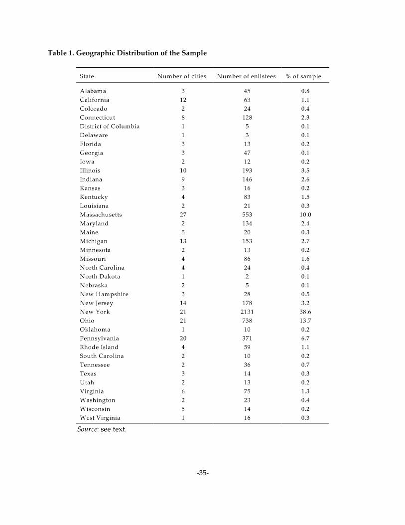
Table 1 describes the geographic distribution of our sample. Thirty-nine percent of the

enlistees were from 21 cities across New York State, with the majority of those coming from

New York City. Fourteen percent of the sample resided in 21 cities across the state of Ohio,

while ten percent came from 27 cities in Massachusetts. Nearly seven percent of the enlistees

-19-

came from 20 twenty towns spread across Pennsylvania, though more were from Philadelphia

and Pittsburgh. Illinois and Indiana claimed 3.5 and 2.6 percent of the sample respectively.

While these numbers suggest the sample draws heavily from a few states, these states are not

limited to a specific region, and even states with relatively small sample shares contain a

significant number of enlistees in absolute numbers. For example, just over 1 percent of the

sample was from California which translates into 63 enlistees. Similarly, 1.4 percent of the

sample, or 75 enlistees, came from Virginia; seven-tenths of 1 percent, or 36 enlistees, came

from Tennessee; and four-tenths of 1 percent, or 23 enlistees, came from Washington state.

If one looks at the spatial distribution of enlistees across cities rather than states, the

patterns are not altered in any meaningful way. In particular, the sample includes enlistees

from 230 cities. The median city contains 9 enlistees; the mean city contains 24. The cities from

which the greatest number of enlistees came are: Syracuse (42 enlistees); St. Louis (47);

Columbus (49); Youngstown, OH (49); Indianapolis (50); Pittsburgh (53); Rochester (56);

Louisville (57); Toledo (62); Detroit (62); Akron (67); Newark (68); Cincinnati (90); Buffalo (93);

Chicago (119); Baltimore (127); Boston (171); Philadelphia (193); Cleveland (226); and New York

(1,736). Although these cities are predominantly located in the East, Mid-Atlantic, and Midwest

regions, many enlistees also came from cities in the South and West. For example, seven came

from Sioux City, ND; ten came from Oklahoma City; ten came from Salt Lake City; sixteen

came from Memphis; twenty came from Denver; twenty came from New Orleans; twenty-

seven came from Birmingham, AL; came twenty-seven from Richmond, VA; twenty-seven

-20-

came from Los Angeles; and thirty-two came from Atlanta. As Figure 7 shows, overall city

population was a primary determinant of how many enlistees came from a particular city.

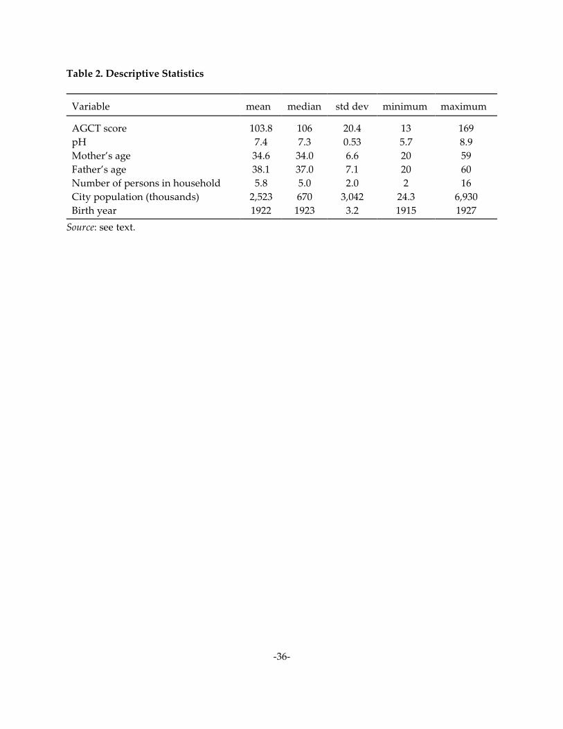
Table 2 provides descriptive statistics for a few key variables. The mean and median

AGCT score of the 5,521 enlistees are 103.8, and 106. As of 1930, the typical enlistee had a

mother and father with an average age of 35 and 38; came from a household with five to six

members; and resided in a city with a mean population of 2.5 million, and a median of 670

thousand. Although enlistees in this sample were born as early as 1915 and as late as 1927, the

typical enlistee was born in 1922 or 1923. Enlistees consumed water that ranged from the

mildly acidic (5.7) to alkaline (8.9), with the typical enlistee drinking water that was almost

perfectly neutral (7.2 or 7.3).

Figure 8 helps frame our estimating procedure. Each observation takes the average

AGCT for enlistees who had consumed water of a given pH level while growing up. Each

observation is labeled with the number of enlistees who consumed water with that pH level.

For example, there were 67 enlistees who drank water with a pH of 5.7. It should be noted that

not all of these enlistees were from the same city or region. Four separate cities in the U.S. had

water with a pH level of 5.7. On the other end of the scale, fourteen enlistees came of age in

areas with water supplies with a pH of 8.9, while 26 lived in areas with a water pH of 8.5. More

than 90 percent of all the enlistees came from areas with drinking water that had a pH level

between 6.5 and 8.5. Yet our analysis is predicated on the relatively small populations on the

tail ends of the water pH distribution (i.e., enlistees who lived in areas with water supplies

with pH less than 6.5 or greater than 8.5). Note, in particular, that there are only forty enlistees

The results reported here do not correct the standard errors for clustering at the city17

level. All of the findings that follow are robust to such clustering.

Because we know the enlistee’s location only at the time of the 1930 Census and at the18

time of his enlistment, we are unable to control for the exact age at which the exposure to

-21-

who grew up drinking water with alkalinity levels of 8.5 or larger. As a result, estimating the

relationship between alkalinity and AGCT scores for highly alkaline water sources will

generate imprecise estimates.

3. Regression Analysis

We estimate variants of the following equation:

i 1 j 2 j i ij(1) y = á + â (pH ) + â (pH ) + ãX + å2

i j iwhere y is the outcome of interest (AGCT score for enlistee i), pH is pH in location j, X is a

ijvector of individual characteristics, and å is an error term with the usual properties. Note that

we include terms for both pH and pH-squared. This specification is motivated by the literature

on water chemistry that inspires Figure 1. Holding everything else constant, we expect to find a

non-monotonic relationship like that in Figure 2 between pH and the AGCT score. The results

do not change if we employ the log of pH and the squared value of the log of pH. Note also

that pH is observed at the city-level, and pH levels do not vary across enlistees from the same

city.17

iThe vector X includes controls for the following characteristics. There are a series of

dummy variables that control for enlistee i’s household size in 1930 (=1 if household contained

n persons, and 0 otherwise; where n = 2-16). Another series of dummy variables control for the

enlistee’s year of birth; for mother’s and father’s literacy status; state dummies; race; and18

water-borne lead occurred. This would be useful, as the effect of exposure differs by the age at

which exposure took place.

In particular, we include age and age-squared for both mother and father. For19

observations where father’s or mother’s age was missing from the Census file, we included a

dummy variable indicating that. Ages for both parents are censored from below at 20 and

from above at 60. For mothers and fathers with ages outside these thresholds, the missing

dummy is coded as 1. This coding strategy allows us to retain observations for which reported

ages seem implausible (e.g., a mother or father with an age of 3). If we retain the original

reported age, however implausible, the results do not change. There is reliable age parental

age information for more than 3,000 enlistees.

We have controlled for city size using dummy variables and continuous functions20

with a level and a squared term. The results are robust across these specifications.

-22-

father’s employment status. Continuous measures control for mother’s age and father’s age as

of 1930. We also include the (log of) the population of the city in which the enlistee came of19

age. In order to allow for the possibility that there exists a dose-response relationship between20

lead exposure and AGCT score, we also report results for both the full sample and the subset of

individuals who at the time of their enlistment resided in the same county where they were

observed in 1930 (“persisters”).

Table 3 summarizes our main results. In each specification that includes fixed effects

for state, the anticipated non-linear relationship between pH and AGCT scores is observed.

Using the coefficients on pH for the full sample, the effect of pH on AGCT score is increasing

for pH until pH levels of 7.8 and decreasing thereafter. Using the same coefficients, the implied

impact on AGCT score from moving from pH 5.5 to pH 6 is 4 points, or just under 1/5 standard

deviation. In all regressions including state dummies, an F-test on the joint hypothesis that the

To ensure that the quadratic specification was not overly sensitive to the small21

number of extreme pH observations (pH < 6.5 or pH > 8.5), we conducted the analysis for

persisters in Table 3 without these observations. The results (a large and statistically effect for

both pH and pH ) remained, though only when the standard errors were clustered at the state2

level. The cities at the lower tail of the pH distribution were (pH<6.5), from lowest to highest

pH: Fall River, New Bedford, Taunton, Woonsocket, Warwick, Wilmington, Atlantic City,

Concord, Manchester, Chicopee, Fitchburgh, Haverhill, Holyoke, Lowell, Memphis, Nashua,

Newburyport, Northampton, Boston, Brockton, Brookline, Cambridge, Chelsea, Everett,

Gloucester, Hartford, Lawrence, Lynn, Malden, Medford, Meriden, New Britain, Newton,

-23-

coefficients on pH and pH-squared are both equal to zero yields an F-statistic which is

significantly from zero at the 2 percent level or higher.

In the last two columns, attention is restricted to individuals whose county of

enlistment was the same as the county in which they were enumerated in the 1930 census

(labeled “Persisters”). This is done to assess the dose-response relationship by focusing on

individuals whose time of exposure at the 1930 location was longer (individuals who migrated

out of their 1930 location may have moved to either rural places, urban places with lower pH,

or urban places with higher pH–we assume that non-migration did not occur in a way that was

systematically correlated with IQ or water pH at the 1930 location or location at enlistment). In

each case where state fixed effects were used, the regression on persisters produced a larger

effect than the corresponding regression using all observations. The estimates for the persisters

are also more precise. The implied effect on AGCT in moving from pH 5.5 to pH 6 is 4.7 points,

0.7 points larger than the effect when persisters and migrants were examined together.

Together, these results suggest that pH and lead exposure were associated with AGCT, the

effect was non-linear (positive for low pH and negative for high pH), and the effect was greater

with longer exposure.21

Norwich, Pawtucket, Providence, Salem, Somerville, Vicksburg, Waltham, Waterbury, and

Worcester. The cities at the upper tail of the pH distribution were (pH>8.5), from lowest to

highest pH: South Bend, Baton Rouge, Berkeley, Oakland, and San Francisco

The sample size is reduced because not all states were part of both the Death22

Registration Area and the Birth Registration Area established by the U.S. Census Bureau. The

infant mortality rates (per thousand) are reported in U.S. Census Bureau (1920-1927).

-24-

One important potentially confounding factor is the disease environment in the city and

year of birth for the enlistee. Eppig et al. (2010) have found evidence at the aggregate level

(using countries as units of observation) that the disease burden (measured by prevalence of

parasites) is negatively related to average IQ levels. Bleakley (2007) finds that individuals who

were young at the time of the hookworm eradication campaign in the early twentieth century

Southern U.S. had higher levels of school attendance as children and higher incomes as adults

than those who were not exposed to the campaign. Figure 9 shows a scatterplot of the raw

data, and a negatively-sloped regression line, for the infant mortality rate and the AGCT score.

To account for the possibility that the local disease environment is linked to later-life

intelligence, Table 4 replaces the pH of the local water supply with the infant mortality rate for

the city and year in which the enlistee was born. For both the full sample and persisters only,22

the infant mortality rate was associated with a lower AGCT score at enlistment. A difference of

50 per thousand was associated with a difference of 3.5 points on the AGCT test. Table 5 uses

both pH and the infant mortality rate together. It shows that the magnitudes of both are similar

to when they were entered separately, and for persisters, are statistically significant.

The regressions in Tables 6 and 7 show that the relationship between pH and AGCT

score is positive for pH # 7, but negative for pH $ 7.5, regardless of whether the infant

Note, however, that while the choice of threshold is robust for the lower knot (e.g.,23

points around 7), the threshold for the upper knot is sensitive to specification. If, for example,

we estimate the model with observations of 7.5 or higher, the coefficient on pH is positive,

though insignificant. The same holds true if we restrict the sample to observations with a pH of

8.2 or higher. The failure to find a robust relationship at the upper end of the litmus scale

reflects, as noted above, a limited amount of variation.

Another possible confounding factor is lead exposure through media other than water24

(e.g. from paint, leaded gasoline, or other air-borne sources such as lead smelters or burning

coal). None of these sources would produce the observed relationship between water pH levels

and AGCT scores. In addition, leaded gasoline was introduced only in 1924, so enlistees would

have been exposed to little lead from this source. The greatest exposure to lead from smelters

in the 1920s came in rural places near the source where lead was mined (an important

exception being the ASARCO smelter on the eastern edge of Omaha which operated from the

1880s through the 1980s and remains an EPA priority clean-up site. Secondary lead smelters

(which processed automobile batteries) became common (with some of them in cities) only in

the late 1930s as the first generations of mass-produced automobiles aged out of use. It seems

reasonable to assume that exposure from factors such as paint, food, coal-fired heating (which

most cities had in some form) and perhaps even automobiles did not vary greatly across cities

(except for possible differences in the use of coal heating by climatic region). This assumption

seems less plausible, however, if we move to industrial sources of pollution. In future work, we

hope to address this concern in greater detail.

-25-

mortality rate is included. This is consistent with the relationship between lead take-up and pH

shown in Figure 1: for pH below 7, high pH results in less lead take-up and therefore less

cognitive impairment and higher AGCT; for pH above 7.5, high pH results in more take-up,

more impairment, and lower AGCT. Table 8 allows for a still more flexible specification: it23

allows the intercept and slope of the pH-AGCT relationship to vary by the pH level, consistent

with the relationship in Figure 2. The pH coefficient is positive for low pH (< 7) and essentially

zero for higher pH levels.24

Figure 10 provide a visual depiction of our results and help clarify the estimation issues

raised in Table 3. To construct this figure, we predicted AGCT scores for non-

-26-

movers/persisters, excluding the pH and pH-squared terms. We then calculated the residual

for each of the enlistees and calculated an average residual for every city in our data set that

had one or more enlistees. The average residual AGCT score for each city is plotted against the

pH level, and a line is fit to highlight the trend relationship. This is done at the city level rather

than the enlistee level because pH levels are observed at the city level. The “polynomial” curve

is the residual pattern regressed against the city-level pH and pH . Observations are weighted2

by the number of enlistees from each city. The “smoothed” curve is estimated using STATA’s

running line smoother (lowess option, bandwidth of .3), which imposes no structure on the

residuals, as opposed to the polynomial. Nevertheless, the same basic pattern is observed: low

pH is associated with low residuals, medium pH with high residuals, and high pH with low

residuals. The polynomial estimate in Figure 10 shows that moving from a pH level of 5.5 to a

pH level of 7.5 results in a gain of roughly 2.5 AGCT points.

Conclusions

The effect of lead exposure in urban water systems in the early twentieth century has

been difficult to assess. The effect of lead on cognitive functioning is well known, but we have

few direct measures of cognitive functioning in large populations that allow us to distinguish

individuals likely exposed to lead in water from those not exposed. At the same time, in

modern populations, it is possible that the lead-intelligence link can be contaminated by

selection effects or unobserved heterogeneity. We have taken advantage of new data linking

World War Two U.S. Army enlistees (whose IQ was measured at enlistment using the AGCT)

to the households in which they resided in 1930 to address these concerns.

-27-

Our study has a number of shortcomings, the fist of which is the lack of an exact

mapping from our intelligence measure (the AGCT score) to IQ which has been used in most

modern studies of the lead-intelligence link. Though AGCT and IQ are highly correlated, the

correlation is not perfect. A second problem is our reliance on modern measures of water pH

levels, when what we really need is pH in the 1920s and 1930s. Finally, though we have a rich

set of covariates, there remain some sources of unobserved individual heterogeneity that can

influence measured intelligence (genetic factors, the amount of intellectual stimulation

provided in the household environment).

Nonetheless, our analysis provides strong evidence of a link between lead exposure and

intelligence for a large population. Those residing in 1930 in cities with higher pH levels but

levels below 6.5 had higher AGCT scores than those in places with lower pH levels; at high pH

levels (greater than 8), increased pH reduced AGCT score. This non-linearity is consistent with

what we know about how pH influences the amount of lead taken up by water traveling

through lead pipes and fixtures: take up falls with pH at low pH levels and rises with pH at

high pH levels. When individuals who remained in the same location between 1930 and

enlistment in the Army were examined separately, their effects were greater (both larger in

magnitude and more precisely estimated), suggesting the existence of a strong dose-response

relationship in lead exposure. These results are consistent with the pervasive use of lead in

urban water systems in the early twentieth century, the interaction between water chemistry

and lead exposure, and lead’s effect on cognitive ability.

-28-

One implication of these findings is that even into their twenties, individuals exposed to

low levels of water-borne lead can exhibit diminished intellectual capacity. Another is that the

total societal costs of lead water pipes greatly exceed the short-run costs in infant mortality and

lead poisoning at the time of exposure – these costs for an individual may be manifested over

an entire lifetime in diminished intellectual functioning, reduced levels of education, and lower

income. Finally, our work here sets the stage for actually quantifying those costs: we are in the

process of linking enlistees to measures of their later-life income and disability levels and death

records to better assess how the costs of early-life exposure accumulate over an entire lifetime.

References

Adams, H., 1852. On the Action of Water on Lead Pipes, and the Diseases Proceeding From It.

Transactions of the American Medical Association 5, 165-236.

Baker, M.N., 1897. The Manual of American Waterworks. New York: The Engineering News.

Baum, C.R., Shannon, M.W., 1997. The lead concentration of reconstituted infant formula, of

Clinical Toxicology 35, 371-375.

Bingham, W.V., 1946. Inequalities in Adult Capacity – From Military Data. Science 104, 147-152.

Bingham, W.V., 1952. A history of psychology in autobiography, Vol. 4. Worcester, MA: Clark

University Press.

Bleakley, H., 2007. Disease and Development: Evidence from Hookworm Eradication in the

American South. Quarterly Journal of Economics 122, 73-117.

Borja-Aburto, V.H., Hertz-Picciotto, I., Rojas Lopez, M., 1999. Blood Lead Levels Measured

Prospectively and Risk of Spontaneous Abortion. American Journal of Epidemiology

150, 590-97.

Boston Water Commissioners, 1848. Report of the Water Commissioners on the Material Best

Adapted for Distribution Water Pipes; and On the Most Economical Mode of

Introducing Water into Private Houses. Boston: J.H. Eastburn, City Printer.

-29-

Bradley, G.H., 1949. A Review of Educational Problems Based on Military Selection and

Classification Data in World War. Journal of Educational Research 43, 161-174.

Canfield, R.L., Henderson, C.R., Cory-Schlecter, D.A., 2003. Intellectual Impairments in

Children With Blood Lead Concentrations Below 10 micrograms per Deciliter. New

England Journal of Medicine 348, 1517-26.

Cardew, P.T., 2003. A Method for Assessing the Effect of Water Quality Changes on

Plumbosolvency Using Random Daytime Sampling. Water Research 37, 2821-32.

Centers for Disease Control and Prevention, 2005. Preventing Lead Poisoning in Young

Children. Atlanta: CDC.

Centers for Disease Control and Prevention, 2010. Guidelines for Identification and

Management of Lead Exposure in Lactating Women. Atlanta: CDC.

Christison, R., 1844. On the Action of Water on Lead. Transactions of the Royal Society of

Edinburgh 15, 265-76.

Clay, K., Troesken, W., Haines, M., 2010. Lead, Mortality, and Productivity. National Bureau of

Economic Research Working Paper 16480. Cambridge: NBER.

Coffigny, H., Thoreaux-Manley, A., Pinon-Lataillade, G., Monchaux, G., Masse, R., Soufir, J.C.,

1994. Effects of Lead Poisoning of Rats During Pregnancy on the Reproductive System

and Fertility of Their Offspring. Human and Experimental Toxicology 13, 241-46.

Committee on Service Pipes, New England Water Works Association, 1917. Report of the

Committee on Service Pipes. Presented to the Association on March 14, 1917. Reprinted

in the Journal of the New England Water Works Association 31, 323-389.

Counter, S.A., Buchanan, L.H., 2004. Mercury exposure in children: a review. Toxicology and

Applied Pharmacology 198, 209–230.

Davidson, C.M., Peters, N.J., Britton, A., 2004. Surface Analysis and Depth Profiling of

Corrosion Products Formed in Lead Pipes Used to Supply Low Alkalinity Drinking

Water. Water Science and Technology 49, 49-54.

Davis, R.B., Anderson, D.S., Norton, S.A., Ford, J., Sweets, P.R., Kahl, J.S., 1994. Sedimented

diatoms in northern New England lakes and their use as pH and alkalinity indicators.

Canadian Journal of Fisheries and Aquatic Sciences 51, 1855-1876.

-30-

Durfour, C.N., Becker, E., 1964. Public Water Supplies of the 100 Largest Cities in the United

States, 1962. Washington, DC: GPO.

Eppig, C., Fincher, C.L., Thornhill, R., 2010. Parasite prevalence and the worldwide distribution

of cognitive ability. Proceedings of the Royal Society, Series B 277, 3801-3808.

Gangoso, L., Alvarez-Lloret, P., Rodriguez-Navarro, A.A., Mateo, R., Hiraldo, F.,Donázar, J.A.,

2009. Long-Term Effects of Lead Poisoning on Bone Mineralization in Vultures Exposed

to Ammunition Sources. Environmental Pollution 157, 569-74.

Gould, S.J., 1982. A Nation of Morons. New Scientist 94, 349-358.

Gulson, B.L., Mahaffey, K.R., Jameson, C.W,. Mizon, K.J., Korsch, M.J., Cameron M.A., 1998.

Mobilization of lead from the skeleton during the postnatal period is larger than during

pregnancy. Journal of Laboratory and Clinical Medicine 131, 324-329.

Gulson, B.L,. Mizon, K.J., Palmer, J.M., Patison, N., Law, A.J., Korsch, M.J., 2001. Longitudinal

study of daily intake and excretion of lead in newly born infants. Environmental

Research 85, 232-245.

Halem, N.B., West, J.R., Forster, C.F., 2001. The Potential for Biofilm Development in Water

Distribution Systems. Water Research 35, 4063-71.

Hamilton, A., United States, Department of Labor. Bureau of Labor Statistics, 1919. Women in

the Lead Industries. Bulletin 253. Washington, D.C.: Government Printing Office.

Karpinos, B.D., 1958. Height and Weight of Selective Service Registrants Processed for Military

Service During World War II. Human Biology 30, 292-321.

Journal of the American Medical Association, 1942. Queries and Minor Notes: Lead Pipe for

Connection Between Water Main and Residence. Journal of the American Medical

Association 120, 995.

Kerr, S., Newell, R.G., 2003. Policy-Induced Technology Adoption: Evidence from the U.S. Lead

Phasedown. Journal of Industrial Economics 51, 317-43.

Harrell, T.W. (1992). Some History of the Army General Classification Test. Journal of Applied

Psychology 77, 875-878.

-31-

Hilton, F., Hank, G., Levinson, A., 1998. Factoring the Environmental Kuznets Curve: Evidence

from Automotive Lead Emissions. Journal of Environmental Economics and

Management 35, 126-41.

Kirkwood, J.P. (ed.), 1859. Collection of Reports and Opinions of Chemists in Regard to the Use

of Lead Pipe for Service Pipe, in the Distribution of Water for the Supply Cities. New

York: Hosford and Company.

Lanphear, B.P., Dietrich, K., Auninger, P., Cox, C., 2000. Cognitive Deficits Associated With

Blood Lead Concentrations < 10 microg/dL in U.S. Children and Adolescents. Public

Health Reports 115, 521-29.

Lanphear,B.P., Hornung, R., Khoury, J., Yolton, K., Baghurst, P., Bellinger, D.C., Canfield, R.L.,

Dietrich, K.N., Bornschein, R., Greene, T., Rothenberg, S.J., Needleman, H.L., Schnaas,

L., Wasserman, G., Graziano, J., Roberts, R., 2005. Low-Level Environmental Lead

Exposure and Children’s Intellectual Function: An International Pooled Analysis.

Environmental Health Perspectives 113, 894-899.

Levin, E.D., Bowman, R.E., 1988. Long-Term Effects of Chronic Postnatal Lead Exposure on

Delayed Spatial Alternation in Monkeys. Neurotoxicology and Teratology 10, 505-10.

Lindsay, L., 1859. On the Action of Hard Waters upon Lead. Edinburgh New Philosophical

Journal 9, 245-58 and 10, 8-25.

Manton, W.I., Angle, C.R., Stanek, K.L., Reese, Y.R., Kuehnemann, T.J., 2000. Acquisition and

retention of lead by young children. Environmental Research 82, 60-80.

Manton, W.I., Angle, C.R,. Stanek, K.L,. Kuntzelman, D., Reese, Y.R,. Kuehnemann, T.J., 2003.

Release of lead from bone in pregnancy and lactation. Environmental Research 92,

139-151.

McGivern, R.F., Sokol, R.Z., Berman. N.G., 1991. Prenatal Lead Exposure in the Rat During the

Third Week of Gestation: Long-Term Behavioral, Physiological, and Anatomical Effects

Associated with Reproduction. Toxicology and Applied Pharmacology 110, 206-15.

Melosi, M.V., 2002. The Sanitary City. Baltimore: Johns Hopkins University Press.

Moore, M.R., Hughes, M.A., Goldberg, D.J., 1979. Lead Absorption in Man from Dietary

Sources: The effect of cooking upon lead concentrations of certain foods and beverages.

International Archives of Occupational and Environmental Health 44, 81-90.

-32-

National Archives and Records Administration, 2002. World War II Army Enlistment Records.

Record Group 64.

Needleman, H.L., 1998. Clair Patterson and Robert Kehoe: Two Views on Lead Toxicity.

Environmental Research 78, 79-85.

Needleman, H.L., 2000. The Removal of Lead from Gasoline: Historical and Personal

Reflections. Environmental Research 84, 20-25.

Needleman, H.L., 2004. Lead Poisoning. Annual Review of Medicine 55, 209-22.

Needleman, H.L., 2009. Low Level Lead Exposure: History and Discovery. Annals of

Epidemiology 19, 235-38.

Needleman, H.L., Schell, A., Bellinger, D., 1990. The Long-Term Effects of Exposure to Low

Doses of Lead in Childhood: An Eleven-Year Follow Up Report. New England Journal

of Medicine 322, 83-88.

Oliver, T., 1914. Lead Poisoning: From the Industrial, Medical, and Social Points of View.

London: H.K. Lewis.

Parkes, L., Kenwood, H., 1901. Hygiene and Public Health. Philadelphia: P. Blakiston’s Son.

Pierrard, J.-C., Rimbault, J., Aplincourt, M., 2002. Experimental Study and Modelling of Lead

Solubility as a Function of pH in Mixtures of Ground Waters and Cement Waters. Water

Research 36, 879-90.

Reyes, J.W., 2007. Environmental Policy as Social Policy? The Impact of Childhood Lead

Exposure on Crime. B.E. Journal of Economic Analysis and Policy: Contributions to

Economic Analysis and Policy 7, Issue 1, Article 51.

Roy, A., Hu, H., Bellinger, D.C., Mukherjee, B., Modali, R., Nasaruddin, K., Schwartz, J.,

Wright, R.O., Ettinger, A.S., Palaniapan, K., Balakrishnan, K., 2011. Hemoglobin, Lead

Exposure, and Intelligence Quotient: Effect Modification by the DRD2 Taq IA

Polymorphism. Environmental Health Perspectives 119, 144-149.

Ruggles, S., Alexander, J.T., Genadek, K., Goeken, R., Schroeder, M.B., Sobek, M., 2010.

Integrated Public Use Microdata Series: Version 5.0 [Machine-readable database].

Minneapolis: University of Minnesota.

Schindler, D.W. (1988). Effects of Acid Rain on Freshwater Ecosystems. Science 239,149-157.

-33-

Schock, M., 1990. Causes of Temporal Variability of Lead in Domestic Plumbing Systems.

Environmental Monitoring and Assessment 15, 59-82.

Simmons, T., 1993. Lead-Calcium Interactions in Cellular Lead Toxicity. Neurotoxicology 14,

77-85.

Sisson, E.D., 1948. Chapter IV: The Personnel Research Program of the Adjutant General's

Office of the United States Army. Review of Educational Research 18, 575-614.

Staff, Personnel Research Section, Adjutant General's Office, 1945. The Army General

Classification Test. Psychological Bulletin 42, 760-768.

Staff, Personnel Research Section, Adjutant General's Office, 1947. The Army General

Classification Test, with special reference to the construction and standardization of

Forms 1a and 1b. Journal of Educational Psychology 38, 385–420.

Stewart, W.F., Schwartz, B.S., 2007. Effects of Lead on the Adult Brain: a 15 Year Exploration.

American Journal of Industrial Medicine 50, 729-39.

Tamminen, A.W., 1951. A Comparison of the Army General Classification Test and the

Wechsler Bellevue Intelligence Scales. Educational and Psychological Measurement 11,

646-655.

Thresh, J.C. 1905. A Series of Cases of Lead Poisoning Due to Hard Water. Lancet, October 7,

1033-34.

Thresh, J.C. Beale, J.F., 1925. The Examination of Waters and Water Supplies. Philadelphia: P.

Blakiston’s Son,.

Troesken, W., 2006. The Great Lead Water Pipe Disaster. Cambridge, MA.: MIT Press.

U.S. Census Bureau, 1922-27. Birth, Stillbirth, and Infant Mortality Statistics for the Birth

Registration Area, 1922-27. Washington: GPO.

U.S. Department of Labor, Bureau of Labor Statistics, Cost of Living Division, 1935-36, Study of

Consumer Purchases in the United States, 1935-1936 [Computer file]. ICPSR08908-v3.

Ann Arbor, MI: Inter-university Consortium for Political and Social Research

[distributor], 2009-06-29. doi:10.3886/ICPSR08908

van Der Leer, D., Weatherhill, N.P., Sharp, R.J., 2002. Modelling the Diffusion of Lead into

Drinking Water. Applied Mathematical Modelling 26, 681-99.

-34-

War Department (U.S.), 1943. Machine Records Operation. War Department Technical Manual

12-305, May 1, 1943.

Warren, C., 2000. Brush with Death: A Social History of Lead Poisoning. Baltimore: Johns

Hopkins University Press.

Woodbury, R.M., 1925. Causal factors in infant mortality a statistical study based on

investigations in eight cities. New York: Bureau Publication, United States Children's

Bureau.

Wright, R.O., Tsaih, S.W, Schwartz, J., Wright, R.J., Hu, H., 2003. Association between iron

deficiency and blood lead level in a longitudinal analysis of children followed in an

urban primary care clinic. Journal of Pediatrics 142, 9-14.

Xintaras, C., 1992. Impact of Lead Contaminated Soil on Public Health: An Analysis Paper. U.S.

Department of Health and Human Services, Agency for Toxic Substances and Disease

Registry, Atlanta, GA.

-35-

Table 1. Geographic Distribution of the Sample

State Number of cities Number of enlistees % of sample

Alabama

California

Colorado

Connecticut

District of Columbia

Delaware

Florida

Georgia

Iowa

Illinois

Indiana

Kansas

Kentucky

Louisiana

Massachusetts

Maryland

Maine

Michigan

Minnesota

Missouri

North Carolina

North Dakota

Nebraska

New Hampshire

New Jersey

New York

Ohio

Oklahoma

Pennsylvania

Rhode Island

South Carolina

Tennessee

Texas

Utah

Virginia

Washington

Wisconsin

West Virginia

3

12

2

8

1

1

3

3

2

10

9

3

4

2

27

2

5

13

2

4

4

1

2

3

14

21

21

1

20

4

2

2

3

2

6

2

5

1

45

63

24

128

5

3

13

47

12

193

146

16

83

21

553

134

20

153

13

86

24

2

5

28

178

2131

738

10

371

59

10

36

14

13

75

23

14

16

0.8

1.1

0.4

2.3

0.1

0.1

0.2

0.1

0.2

3.5

2.6

0.2

1.5

0.3

10.0

2.4

0.3

2.7

0.2

1.6

0.4

0.1

0.1

0.5

3.2

38.6

13.7

0.2

6.7

1.1

0.2

0.7

0.3

0.2

1.3

0.4

0.2

0.3

Source: see text.

-36-

Table 2. Descriptive Statistics

Variable mean median std dev minimum maximum

AGCT score

pH

Mother’s age

Father’s age

Number of persons in household

City population (thousands)

Birth year

103.8

7.4

34.6

38.1

5.8

2,523

1922

106

7.3

34.0

37.0

5.0

670

1923

20.4

0.53

6.6

7.1

2.0

3,042

3.2

13

5.7

20

20

2

24.3

1915

169

8.9

59

60

16

6,930

1927

Source: see text.

-37-

Table 3. Regression Results, Dependent Variable AGCT at Enlistment, Full Sample and

Persisters, Controlling for pH.

Full sample Persisters

Variables Coef p-value Coef p-value

pH

pH2

=1 if Non-white

=1 if <6 persons in household

=1 if 6-8 person household

=1 if 9-16 person household

=1 if > 16 person household

Log(city population)

=1 if 1914 birth

=1 if 1915 birth

=1 if 1916 birth

=1 if 1917 birth

=1 if 1918 birth

=1 if 1919 birth

=1 if 1920 birth

=1 if 1921 birth

=1 if 1922 birth

=1 if 1923 birth

=1 if 1924 birth

=1 if 1925 birth

=1 if 1926 birth

Father’s age

(Father’s age)2

=1 if father’s age unknown

=1 father literate

Mother’s age

(Mother’s age)2

=1 if mother’s age unknown

=1 mother literate

=1 if father out of LF

=1 if father employed

=1 if father unemployed

=1 if LF status unknown

State dummies

Adjusted R2

Number of observations

30.1

-1.93

-20.7

3.69

-.065

-5.28

omitted

.317

-2.38

-1.60

-1.40

-2.13

-2.12

-3.37

-2.99

-1.51

-4.51

-5.82

-5.71

.615

omitted

.867

-.012

31.8

9.25

.308

-.001

11.9

3.28

omitted

7.09

4.81

8.56

Yes

.134

5,503

.025

.030

.001

.740

.995

.635

omitted

.125

.575

.693

.728

.596

.597

.402

.457

.708

.256

.135

.140

.876

omitted

.006

.002

.001

.001

.001

.001

.005

.340

omitted

.065

.232

.038

35.5

-2.27

-19.5

4.62

.969

-3.97

omitted

.438

-2.79

-1.05

-1.61

-1.89

-2.24

-4.25

-2.92

-.678

-4.48

-5.54

-5.94

.217

omitted

.776

-.011

28.2

7.78

.307

-.001

9.73

1.26

omitted

7.44

4.87

8.71

Yes

.124

5,009

.012

.016

.001

.733

.943

.769

omitted

.042

.518

.801

.694

.643

.585

.300

.476

.869

.266

.162

.131

.957

omitted

.023

.007

.001

.008

.001

.001

.745

.039

omitted

.051

.228

.035

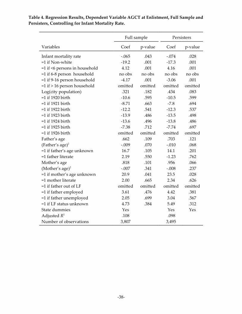
-38-

Table 4. Regression Results, Dependent Variable AGCT at Enlistment, Full Sample and

Persisters, Controlling for Infant Mortality Rate.

Full sample Persisters

Variables Coef p-value Coef p-value

Infant mortality rate

=1 if Non-white

=1 if <6 persons in household

=1 if 6-8 person household

=1 if 9-16 person household

=1 if > 16 person household

Log(city population)

=1 if 1920 birth

=1 if 1921 birth

=1 if 1922 birth

=1 if 1923 birth

=1 if 1924 birth

=1 if 1925 birth

=1 if 1926 birth

Father’s age

(Father’s age)2

=1 if father’s age unknown

=1 father literate

Mother’s age

(Mother’s age)2

=1 if mother’s age unknown

=1 mother literate

=1 if father out of LF

=1 if father employed

=1 if father unemployed

=1 if LF status unknown

State dummies

Adjusted R2

Number of observations

-.065

-19.2

4.12

no obs

-4.17

omitted

.321

-10.6

-8.71

-12.2

-13.9

-13.6

-7.38

omitted

.662

-.009

16.7

2.19

.818

-.007

20.9

2.00

omitted

3.61

2.05

4.73

Yes

.108

3,807

.043

.001

.001

no obs

.001

omitted

.182

.595

.663

.541

.486

.496

.712

omitted

.109

.070

.105

.550

.101

.341

.041

.665

omitted

.476

.699

.384

-.074

-17.3

4.16

no obs

-3.06

omitted

.434

-10.5

-7.8

-12.3

-13.5

-13.8

-7.74

omitted

.703

-.010

14.1

-1.23

.956

-.008

23.5

2.34

omitted

4.42

3.04

5.49

Yes

.098

3,495

.028

.001

.001

no obs

.001

omitted

.083

.599

.694

.537

.498

.486

.697

omitted

.121

.068

.201

.762

.066

.237

.028

.626

omitted

.381

.567

.312

Yes

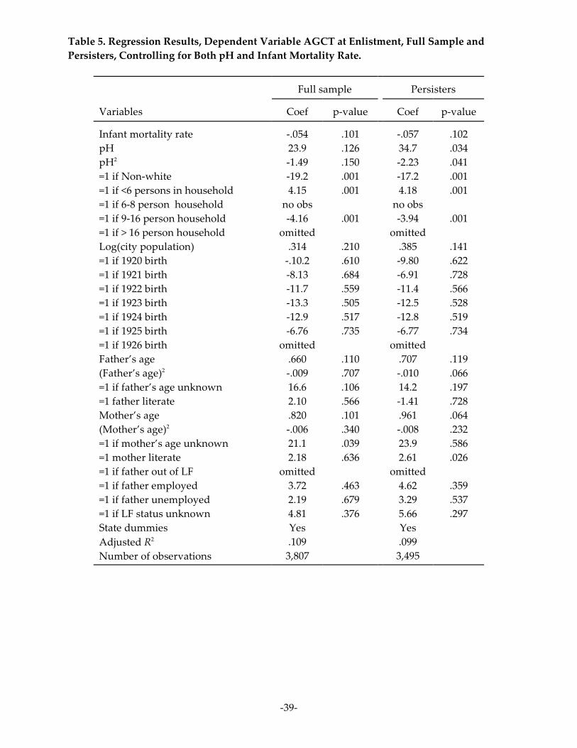
-39-

Table 5. Regression Results, Dependent Variable AGCT at Enlistment, Full Sample and

Persisters, Controlling for Both pH and Infant Mortality Rate.

Full sample Persisters

Variables Coef p-value Coef p-value

Infant mortality rate

pH

pH2

=1 if Non-white

=1 if <6 persons in household

=1 if 6-8 person household

=1 if 9-16 person household

=1 if > 16 person household

Log(city population)

=1 if 1920 birth

=1 if 1921 birth

=1 if 1922 birth

=1 if 1923 birth

=1 if 1924 birth

=1 if 1925 birth

=1 if 1926 birth

Father’s age

(Father’s age)2

=1 if father’s age unknown

=1 father literate

Mother’s age

(Mother’s age)2

=1 if mother’s age unknown

=1 mother literate

=1 if father out of LF

=1 if father employed

=1 if father unemployed

=1 if LF status unknown

State dummies

Adjusted R2

Number of observations

-.054

23.9

-1.49

-19.2

4.15

no obs

-4.16

omitted

.314

-.10.2

-8.13

-11.7

-13.3

-12.9

-6.76

omitted

.660

-.009

16.6

2.10

.820

-.006

21.1

2.18

omitted

3.72

2.19

4.81

Yes

.109

3,807

.101

.126

.150

.001

.001

.001

.210

.610

.684

.559

.505

.517

.735

.110

.707

.106

.566

.101

.340

.039

.636

.463

.679

.376

-.057

34.7

-2.23

-17.2

4.18

no obs

-3.94

omitted

.385

-9.80

-6.91

-11.4

-12.5

-12.8

-6.77

omitted

.707

-.010

14.2

-1.41

.961

-.008

23.9

2.61

omitted

4.62

3.29

5.66

Yes

.099

3,495

.102

.034

.041

.001

.001

.001

.141

.622

.728

.566

.528

.519

.734

.119

.066

.197

.728

.064

.232

.586

.026

.359

.537

.297

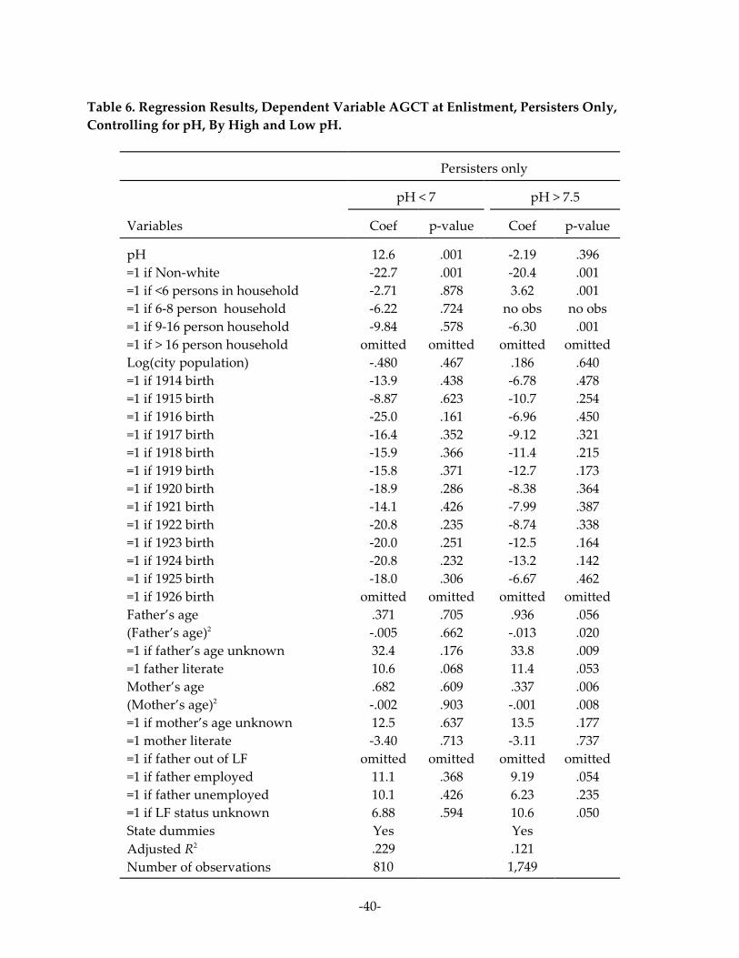
-40-

Table 6. Regression Results, Dependent Variable AGCT at Enlistment, Persisters Only,

Controlling for pH, By High and Low pH.

Persisters only

pH < 7 pH > 7.5

Variables Coef p-value Coef p-value

pH

=1 if Non-white

=1 if <6 persons in household

=1 if 6-8 person household

=1 if 9-16 person household

=1 if > 16 person household

Log(city population)

=1 if 1914 birth

=1 if 1915 birth

=1 if 1916 birth

=1 if 1917 birth

=1 if 1918 birth

=1 if 1919 birth

=1 if 1920 birth

=1 if 1921 birth

=1 if 1922 birth

=1 if 1923 birth

=1 if 1924 birth

=1 if 1925 birth

=1 if 1926 birth

Father’s age

(Father’s age)2

=1 if father’s age unknown

=1 father literate

Mother’s age

(Mother’s age)2

=1 if mother’s age unknown

=1 mother literate

=1 if father out of LF

=1 if father employed

=1 if father unemployed

=1 if LF status unknown

State dummies

Adjusted R2

Number of observations

12.6

-22.7

-2.71

-6.22

-9.84

omitted

-.480

-13.9

-8.87

-25.0

-16.4

-15.9

-15.8

-18.9

-14.1

-20.8

-20.0

-20.8

-18.0

omitted

.371

-.005

32.4

10.6

.682

-.002

12.5

-3.40

omitted

11.1

10.1

6.88

Yes

.229

810

.001

.001

.878

.724

.578

omitted

.467

.438

.623

.161

.352

.366

.371

.286

.426

.235

.251

.232

.306

omitted

.705

.662

.176

.068

.609

.903

.637

.713

omitted

.368

.426

.594

-2.19

-20.4

3.62

no obs

-6.30

omitted

.186

-6.78

-10.7

-6.96

-9.12

-11.4

-12.7

-8.38

-7.99

-8.74

-12.5

-13.2

-6.67

omitted

.936

-.013

33.8

11.4

.337

-.001

13.5

-3.11

omitted

9.19

6.23

10.6

Yes

.121

1,749

.396

.001

.001

no obs

.001

omitted

.640

.478

.254

.450

.321

.215

.173

.364

.387

.338

.164

.142

.462

omitted

.056

.020

.009

.053

.006

.008

.177

.737

omitted

.054

.235

.050

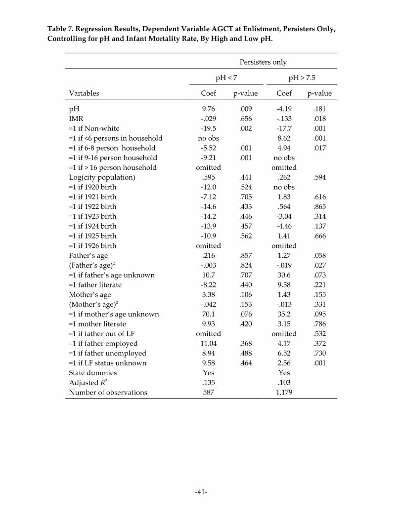
-41-

Table 7. Regression Results, Dependent Variable AGCT at Enlistment, Persisters Only,

Controlling for pH and Infant Mortality Rate, By High and Low pH.

Persisters only

pH < 7 pH > 7.5

Variables Coef p-value Coef p-value

pH

IMR

=1 if Non-white

=1 if <6 persons in household

=1 if 6-8 person household

=1 if 9-16 person household

=1 if > 16 person household

Log(city population)

=1 if 1920 birth

=1 if 1921 birth

=1 if 1922 birth

=1 if 1923 birth

=1 if 1924 birth

=1 if 1925 birth

=1 if 1926 birth

Father’s age

(Father’s age)2

=1 if father’s age unknown

=1 father literate

Mother’s age

(Mother’s age)2

=1 if mother’s age unknown

=1 mother literate

=1 if father out of LF

=1 if father employed

=1 if father unemployed

=1 if LF status unknown

State dummies

Adjusted R2

Number of observations

9.76

-.029

-19.5

no obs

-5.52

-9.21

omitted

.595

-12.0

-7.12

-14.6

-14.2

-13.9

-10.9

omitted

.216

-.003

10.7

-8.22

3.38

-.042

70.1

9.93

omitted

11.04

8.94

9.58

Yes

.135

587

.009

.656

.002

.001

.001

.441

.524

.705

.433

.446

.457

.562

.857

.824

.707

.440

.106

.153

.076

.420

.368

.488

.464

-4.19

-.133

-17.7

8.62

4.94

no obs

omitted

.262

no obs

1.83

.564

-3.04

-4.46

1.41

omitted

1.27

-.019

30.6

9.58

1.43

-.013

35.2

3.15

omitted

4.17

6.52

2.56

Yes

.103

1,179

.181

.018

.001

.001

.017

.594

.616

.865

.314

.137

.666

.058

.027

.073

.221

.155

.331

.095

.786

.532

.372

.730

.001

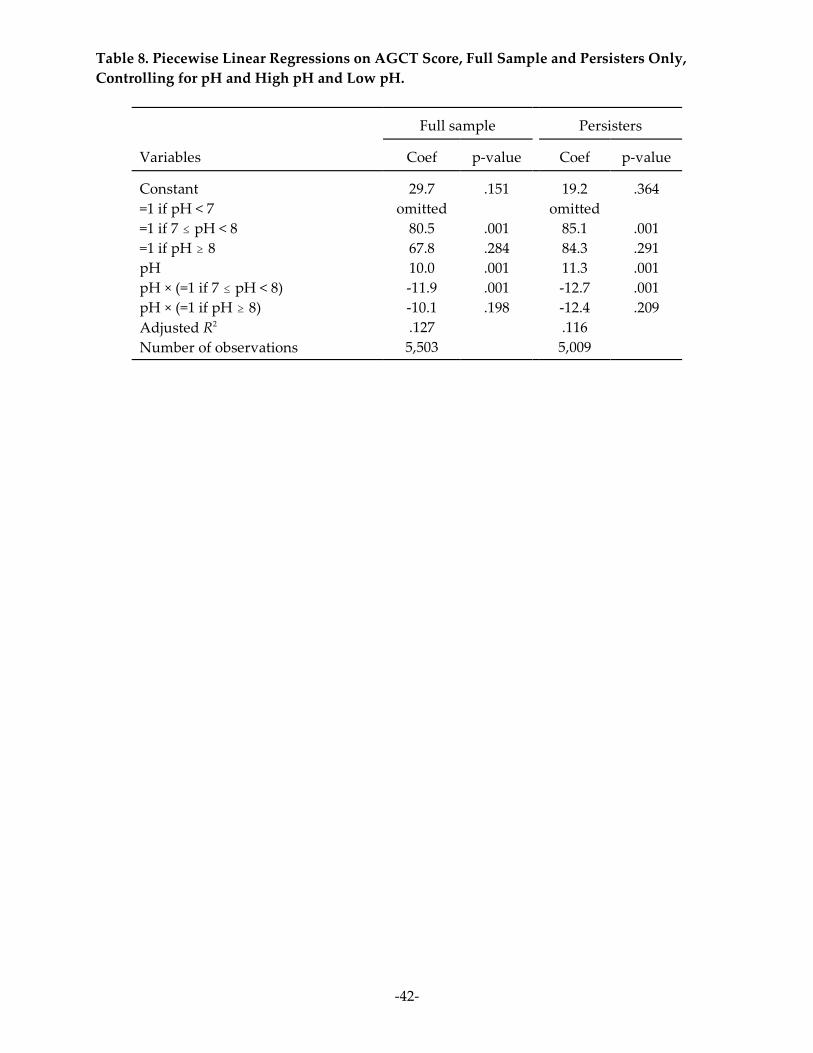
-42-

Table 8. Piecewise Linear Regressions on AGCT Score, Full Sample and Persisters Only,

Controlling for pH and High pH and Low pH.

Full sample Persisters

Variables Coef p-value Coef p-value

Constant

=1 if pH < 7

=1 if 7 # pH < 8

=1 if pH $ 8

pH

pH × (=1 if 7 # pH < 8)

pH × (=1 if pH $ 8)

Adjusted R2

Number of observations

29.7

omitted

80.5

67.8

10.0

-11.9

-10.1

.127

5,503

.151

.001

.284

.001

.001

.198

19.2

omitted

85.1

84.3

11.3

-12.7

-12.4

.116

5,009

.364

.001

.291

.001

.001

.209

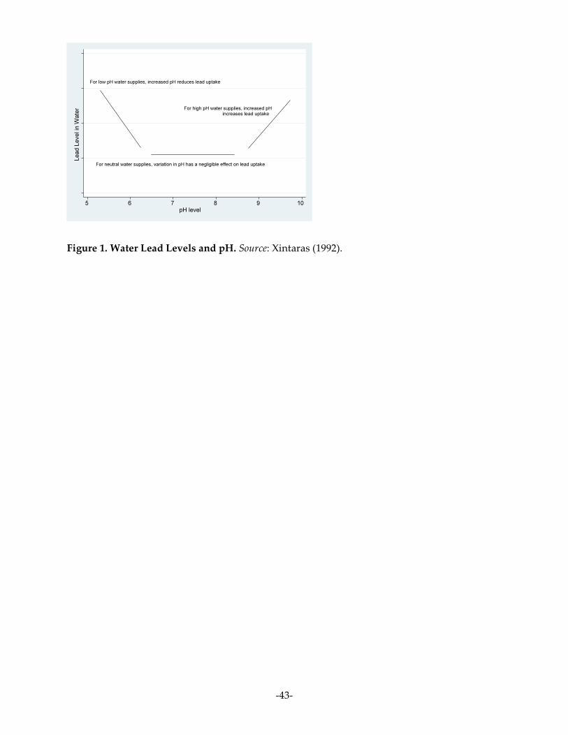
-43-

Figure 1. Water Lead Levels and pH. Source: Xintaras (1992).

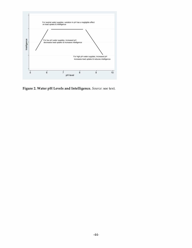
-44-

Figure 2. Water pH Levels and Intelligence. Source: see text.

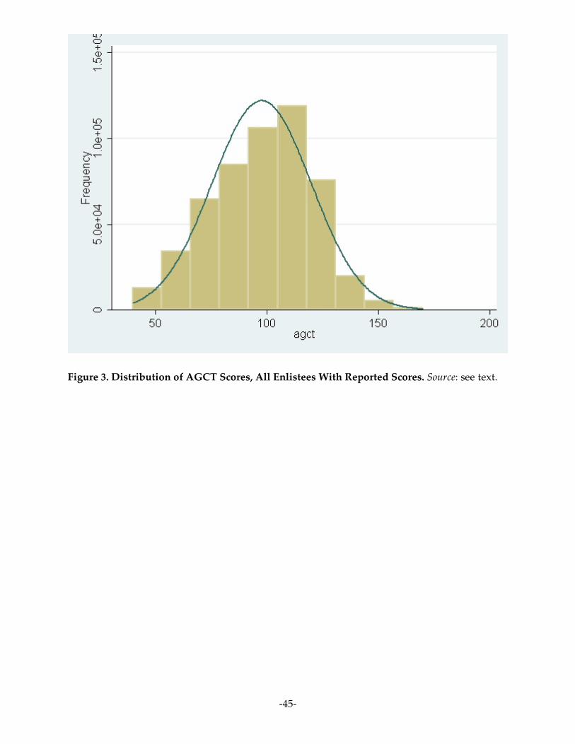
-45-

Figure 3. Distribution of AGCT Scores, All Enlistees With Reported Scores. Source: see text.

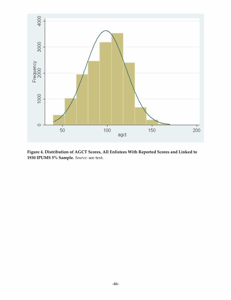
-46-

Figure 4. Distribution of AGCT Scores, All Enlistees With Reported Scores and Linked to

1930 IPUMS 5% Sample. Source: see text.

-47-

Figure 5. Distribution of AGCT Scores, All Enlistees With Reported Scores and Linked to

1930 IPUMS 5% Sample and Located in Cities With Population > 30,000 in 1930. . Source: see

text.

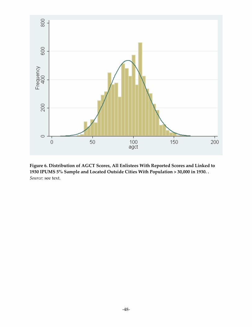
-48-

Figure 6. Distribution of AGCT Scores, All Enlistees With Reported Scores and Linked to

1930 IPUMS 5% Sample and Located Outside Cities With Population > 30,000 in 1930. .

Source: see text.

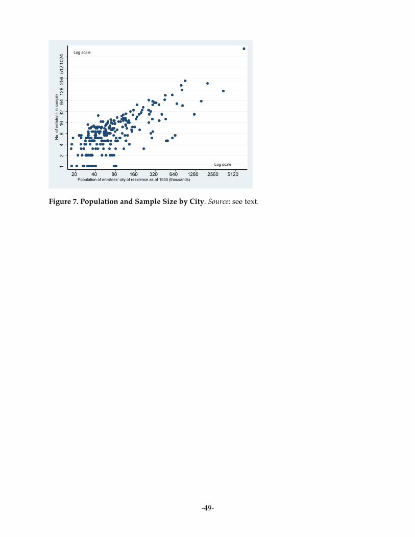
-49-

Figure 7. Population and Sample Size by City. Source: see text.

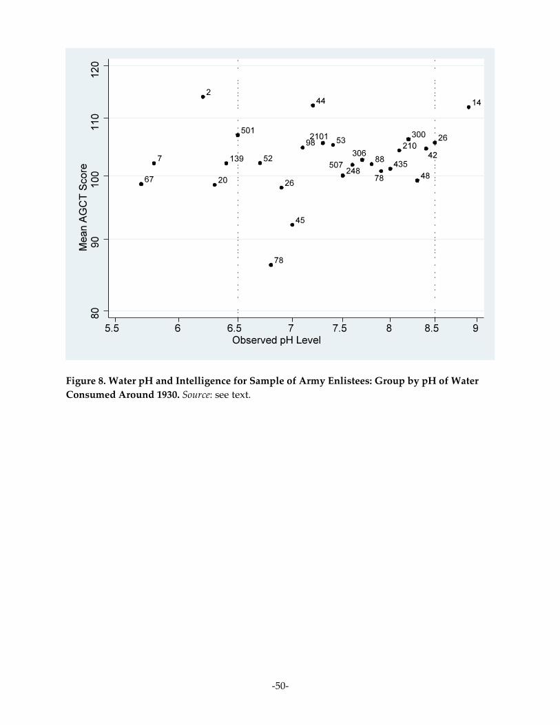
-50-

Figure 8. Water pH and Intelligence for Sample of Army Enlistees: Group by pH of Water

Consumed Around 1930. Source: see text.

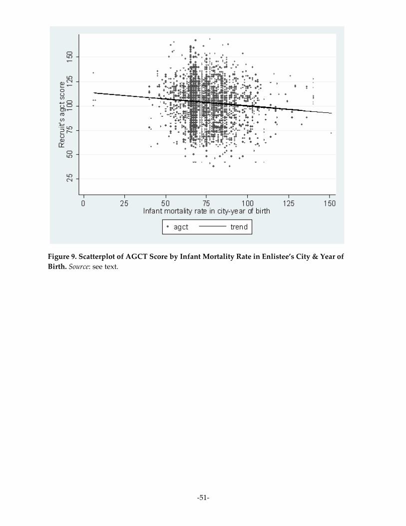
-51-

Figure 9. Scatterplot of AGCT Score by Infant Mortality Rate in Enlistee’s City & Year of

Birth. Source: see text.

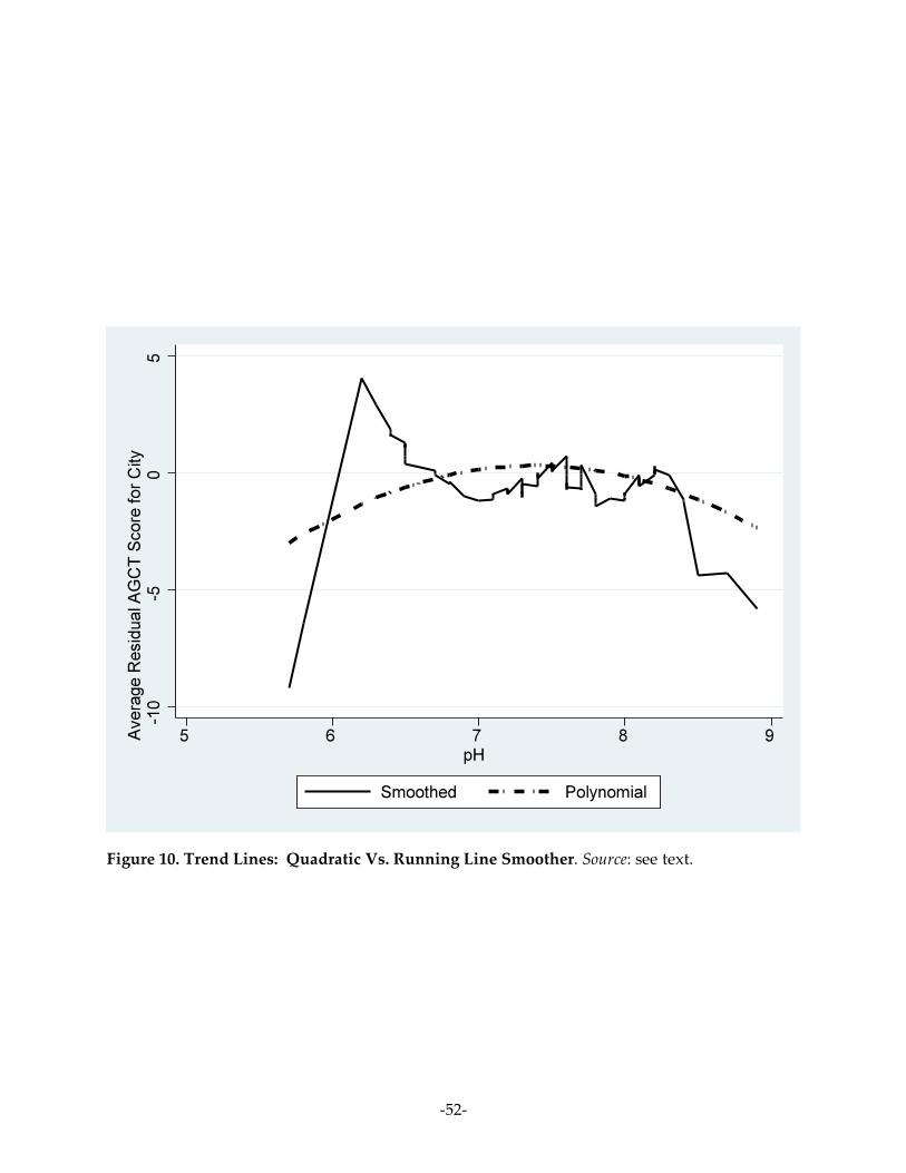
-52-

Figure 10. Trend Lines: Quadratic Vs. Running Line Smoother. Source: see text.