Code Saturne version 5.0 tutorial: Shear Driven …EDF R&D Code Saturne version 5.0 tutorial: Shear...
48
EDF R&D Fluid Dynamics, Power Generation and Environment Department Single Phase Thermal-Hydraulics Group 6, quai Watier F-78401 Chatou Cedex Tel: 33 1 30 87 75 40 Fax: 33 1 30 87 79 16 SEPTEMBER 2017 Code Saturne documentation Code Saturne version 5.0 tutorial: Shear Driven Cavity Flow contact: [email protected] http://code-saturne.org/ c EDF 2017
Transcript of Code Saturne version 5.0 tutorial: Shear Driven …EDF R&D Code Saturne version 5.0 tutorial: Shear...

EDF R&D
Fluid Dynamics, Power Generation and Environment DepartmentSingle Phase Thermal-Hydraulics Group
6, quai WatierF-78401 Chatou Cedex
Tel: 33 1 30 87 75 40Fax: 33 1 30 87 79 16 SEPTEMBER 2017
Code Saturne documentation
Code Saturne version 5.0 tutorial:Shear Driven Cavity Flow
contact: [email protected]
http://code-saturne.org/ c© EDF 2017

EDF R&D Code Saturne version 5.0 tutorial:Shear Driven Cavity Flow
Code Saturnedocumentation
Page 1/47

TABLE OF CONTENTS
I Introduction 3
1 Introduction . . . . . . . . . . . . . . . . . . . . . . . . . . . . . . . . . . . . . . . 4
1.1 Tutorial Components . . . . . . . . . . . . . . . . . . . . . . . . . . . . . . . . . 4
1.2 Tutorial Structure . . . . . . . . . . . . . . . . . . . . . . . . . . . . . . . . . . 4
II Setting up 5
1 Setting up . . . . . . . . . . . . . . . . . . . . . . . . . . . . . . . . . . . . . . . . 6
1.1 What you will learn . . . . . . . . . . . . . . . . . . . . . . . . . . . . . . . . . 6
1.2 Using SALOME CFD together for End-to-End Simulations . . . . . . . . . 6
1.3 Installing SALOME CFD or Code Saturne and SALOME separately . . . . . 6
1.4 Getting Started with End-to-End SALOME/ Code Saturne CFD Simulations 7
III Shear Driven Cavity Flow Case with CFDStudy 11
1 General description . . . . . . . . . . . . . . . . . . . . . . . . . . . . . . . . . . 12
1.1 What You Will Learn . . . . . . . . . . . . . . . . . . . . . . . . . . . . . . . . 12
1.2 Case Description . . . . . . . . . . . . . . . . . . . . . . . . . . . . . . . . . . . 12
1.3 Creating the Code Saturne case . . . . . . . . . . . . . . . . . . . . . . . . . . . . 13
2 Creating the Computational Domain within SALOME . . . . . . . . . . . . . 13
2.1 Geometry . . . . . . . . . . . . . . . . . . . . . . . . . . . . . . . . . . . . . . . . 14
2.2 Meshing . . . . . . . . . . . . . . . . . . . . . . . . . . . . . . . . . . . . . . . . . 20
3 Simulating within SALOME . . . . . . . . . . . . . . . . . . . . . . . . . . . . . 24
3.1 Setting up the CFD Simulation . . . . . . . . . . . . . . . . . . . . . . . . . . . 24
3.2 Running and Analysing the Simulation . . . . . . . . . . . . . . . . . . . . . . 34
3.3 Post-processing the Results . . . . . . . . . . . . . . . . . . . . . . . . . . . . 35
4 References . . . . . . . . . . . . . . . . . . . . . . . . . . . . . . . . . . . . . . . . 47
5 Reference Data from [4] . . . . . . . . . . . . . . . . . . . . . . . . . . . . . . . . 47
2

Part I
Introduction
3

EDF R&D Code Saturne version 5.0 tutorial:Shear Driven Cavity Flow
Code Saturnedocumentation
Page 4/47
1 Introduction1.1 Tutorial Components
This tutorial makes use of:
• The SALOME [1] platform for geometry generation, meshing, and post-processing
• Code Saturne [2], [3] for CFD calculations
• Reference [4] for comparison with published results
To work through this tutorial you will need a computer on which these two software applications arealready available or on which you have permission to install them.
1.2 Tutorial Structure
This tutorial is made of two complementary sections:
• Section II describes all the procedures required to get going with setting up CFD simulationsusing SALOME and Code Saturne, from code download to case creation.
• Section III illustrates setting up, running, and analysing a CFD simulation entirely with SA-LOME and Code Saturne, using the laminar, Shear Driven Cavity as an example. This case issimple but contains enough physics to make it interesting and relevant to practical problems.
If you are already familiar with setting up CFD simulations with Code Saturne and SALOME, youmay skip Section II and go directly to Section III.

Part II
Setting up
5

EDF R&D Code Saturne version 5.0 tutorial:Shear Driven Cavity Flow
Code Saturnedocumentation
Page 6/47
1 Setting upThe first part of the tutorial is designed to explain the preliminary steps to setup an end-to-endCFD simulation using Code Saturne and SALOME and provide an introduction to these softwareapplications.
1.1 What you will learn
In the first part of the tutorial, you will learn:
• How Code Saturne and SALOME may be combined in SALOME CFD for end-to-end CFDanalyses, from CAD generation to post-processing of CFD results
• How to access and download Code Saturne and SALOME
• How to install SALOME and Code Saturne within the CFDStudy module of SALOME
• How to set up a Code Saturne case with CFDStudy
1.2 Using SALOME CFD together for End-to-End Simulations
Code Saturne is a general, 3D CFD solver which can be applied to a large variety of problems involvingfluid flow and heat transfer. The Code Saturne Graphical User Interface (GUI) can be used on its ownto define CFD cases, and to run them when a mesh is already available. It has also been integratedas a module called CFDStudy in the SALOME open-source host platform, where it links with othermodules to provide a single, user-friendly, graphical environment for end-to-end CFD analyses:
• GEOM: CAD module
◦ Geometry and computational domain definition
• SMESH: Meshing module
◦ Surface and volume meshing of the computational domain and defining boundaries
• CFDStudy: CFD module
◦ Set up and run Code Saturne CFD calculations
• Paravis: Post-processing module
◦ Visualisation and analysis with Paraview [5]
The use of the different modules to set-up and run Code Saturne studies is described throughout thedifferent tutorials, starting with how to initiate a study with CFDStudy, as explained in 1.4.
1.3 Installing SALOME CFD or Code Saturne and SALOME sepa-rately
The quickest way to get started is to retrieve a SALOME CFD installer from Code Saturne website:www.code-saturne.org. Then install SALOME CFD by executing the installer in a terminal.
Alternatively, each application, Code Saturne and SALOME, can be installed separately with an optionallowing to integrate Code Saturne inside Salome. Access to the applications is provided through theirrespective, dedicated internet sites. Install utilities, installation instructions, environment variablessetup for Linux installations, and code documentation including user manuals can also be downloadedfrom the sites.
To integrate the Code Saturne and the CFDStudy module in SALOME, SALOME must be installedfirst, followed by Code Saturne:

EDF R&D Code Saturne version 5.0 tutorial:Shear Driven Cavity Flow
Code Saturnedocumentation
Page 7/47
1. SALOME
SALOME can be downloaded from the website: www.salome-platform.org/
Complete versions come with the source and binary files and interactive installation procedures.
2. Code Saturne and CFDStudy module
Code Saturne can be downloaded from the website: www.code-saturne.org
The code is packaged with all its libraries and the installer, which can also be downloadedfrom the same site, makes the installation process fully automatic. However, external, requiredpackages, such as Python, are not part of the Code Saturne package and must be acquired fromtheir respective publishers and installed separately. As part of the installation process, theCode Saturne installer will check for their availability and issue notifications if they are not found.
To enable the CFDStudy module, the --with-salome flag must be added as a parameter to theconfigure command. The flag must point to the path of your SALOME application.
For example: --with-salome=/opt/salome 8.1.0.
Additional information can be found in the installation guide of Code Saturne available on theCode Saturne website.
1.4 Getting Started with End-to-End SALOME/ Code Saturne CFDSimulations
The process of creating the required Code Saturne directory and file structures is decribed first, followedby an example for the Shear Driven Cavity Flow case.
File Structure
Code Saturne makes use of a pre-set directory structure to access and save input and output files.Simulations are organised in terms of studies and cases. Conceptually, a study contains a series ofcases which all rely on the same geometry. The cases represent different instances of simulationsfor this common geometry, for example for different operating conditions. The pre-set Code Saturnedirectory structure can be easily created using the CFDStudy module within SALOME, as describedbelow.
To set up a study and a case, first open the combined interface of Code Saturne and SALOME bytyping the command:
$ code saturne salome
in your terminal. This will start the SALOME platform with the CFDStudy module enabled.
Then, activate CFDStudy, either by selecting it in the module chooser in SALOME’s top tool bar orby clicking on its icon (Figure II.1).
Figure II.1: Opening CFDStudy module
The module’s activation screen will open as shown in Figure II.2.

EDF R&D Code Saturne version 5.0 tutorial:Shear Driven Cavity Flow
Code Saturnedocumentation
Page 8/47
Figure II.2: CFDStudy activation screen.
In the module’s activation screen, select New to create a new study. Then enable CFDSTUDYtoolbar, if it does not appear, in View Toolbars CFDSTUDY . In the toolbar or in the CFDSTUDYmenu, click on Choose an existing CFD study or Create . The study and case creation panel will then pop up(Figure II.3).
Figure II.3: Code Saturne Study and Case Specification. Here a study called EXAMPLE STUDY,containing CASE1, is created
In the panel, choose where you want the study to be stored on your computer and enter the names ofthe study and the first case. Further cases can be added to any study at a later stage. Leave the createMESH directory and create POST directory tick-boxes selected, as this will automatically createthe entire directory structure required by Code Saturne. Press OK to create the study and the case.The Code Saturne directory tree for the study and case will then become visible in the Object Browser,as shown in Figure II.4.
EDF R&D Code Saturne version 5.0 tutorial:Shear Driven Cavity Flow
Code Saturnedocumentation
Page 9/47
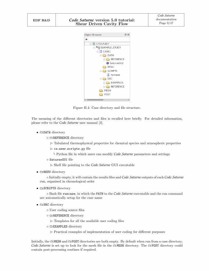
Figure II.4: Case directory and file structure.
The meaning of the different directories and files is recalled here briefly. For detailed information,please refer to the Code Saturne user manual [3].
• DATA directory
◦ REFERENCE directory
� Tabulated thermophysical properties for chemical species and atmospheric properties
� cs user scripts.py file�
Python file in which users can modify Code Saturne parameters and settings
◦ SaturneGUI file
� Shell file pointing to the Code Saturne GUI executable
• RESU directory
◦ Initially empty, it will contain the results files and Code Saturne outputs of each Code Saturnerun, organised in chronological order
• SCRIPTS directory
◦ Bash file runcase, in which the PATH to the Code Saturne executable and the run commandare automatically setup for the case name
• SRC directory
◦ User coding source files
◦ REFERENCE directory
� Templates for all the available user coding files
◦ EXAMPLES directory
� Practical examples of implementation of user coding for different purposes
Initially, the MESH and POST directories are both empty. By default when run from a case directory,Code Saturne is set up to look for the mesh file in the MESH directory. The POST directory couldcontain post-processing routines if required.
EDF R&D Code Saturne version 5.0 tutorial:Shear Driven Cavity Flow
Code SaturnedocumentationPage 10/47
Example: Creating the Shear Driven Cavity Flow Study
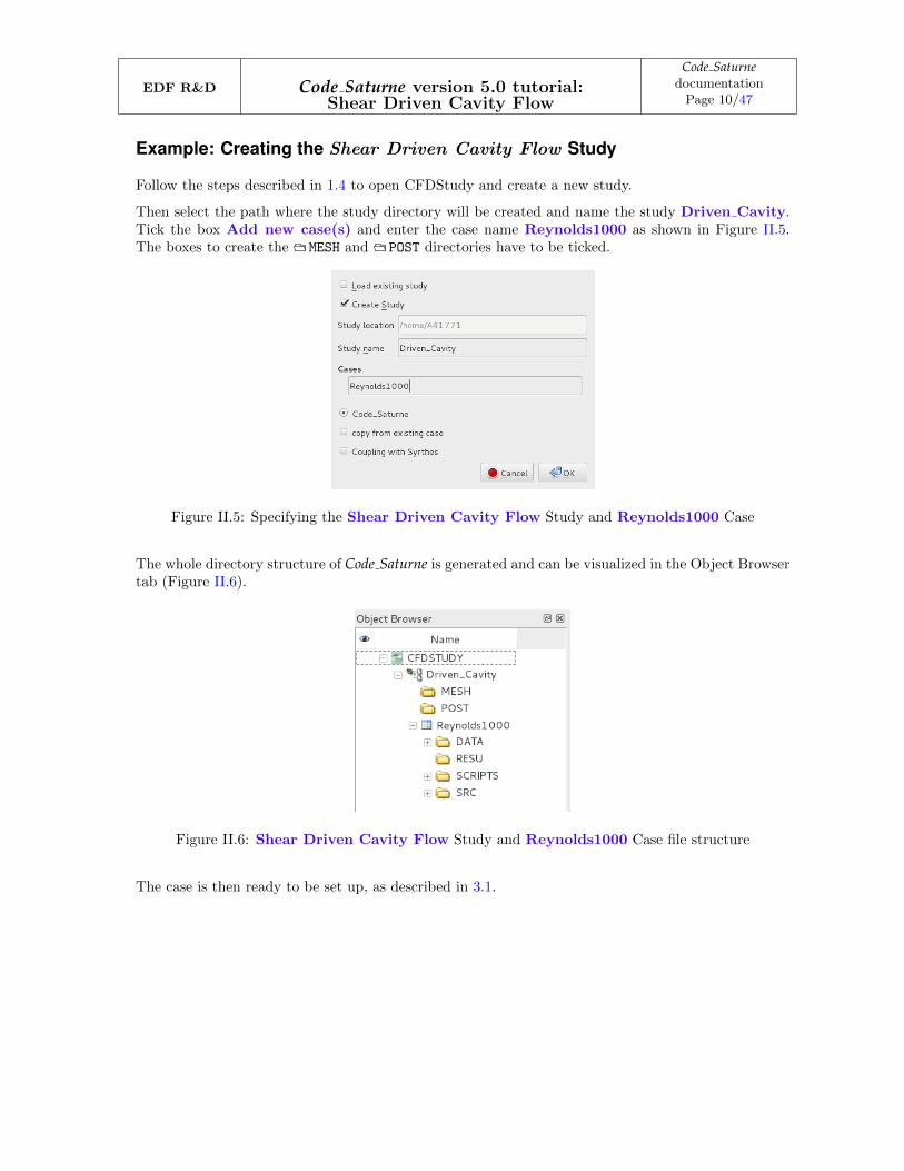
Follow the steps described in 1.4 to open CFDStudy and create a new study.
Then select the path where the study directory will be created and name the study Driven Cavity.Tick the box Add new case(s) and enter the case name Reynolds1000 as shown in Figure II.5.The boxes to create the MESH and POST directories have to be ticked.
Figure II.5: Specifying the Shear Driven Cavity Flow Study and Reynolds1000 Case
The whole directory structure of Code Saturne is generated and can be visualized in the Object Browsertab (Figure II.6).
Figure II.6: Shear Driven Cavity Flow Study and Reynolds1000 Case file structure
The case is then ready to be set up, as described in 3.1.
Part III
Shear Driven Cavity Flow Casewith CFDStudy
11
EDF R&D Code Saturne version 5.0 tutorial:Shear Driven Cavity Flow
Code SaturnedocumentationPage 12/47
1 General descriptionIn the second part of the tutorial, the preparation, simulation and analysis of the Reynolds1000case of the DrivenCavity study is described, from the construction of the computational domain andmesh to the preparation, running and post-processing of the CFD simulation. All the following stepsin this second part are presented using CFDStudy module. However you could also go through thistutorial using Code Saturne and SALOME separately.
1.1 What You Will Learn
Through this tutorial, you will learn how to perform an end-to-end CFD simulation using Code Saturne[2, 3] together with the SALOME [1] platform, from creating the computational domain to analysingthe end results and comparing them with available data. Specifically, you will:
• Create a computational domain with SALOME using available shapes and groups
• Create an hexahedral mesh with different mesh refinements in the X, Y and Z directions withSALOME
• Setup a steady-state, viscous, laminar, isothermal, constant properties fluid CFD simulation withnon-slip walls, a moving wall, and symmetry planes with the CFDStudy module and using theSALOME mesh
• Control and run the Code Saturne simulation from the CFDStudy module
• Examine the Code Saturne output and results files, including data along specified profiles and atmonitoring points
• Analyse and visualise the results with SALOME
1.2 Case Description
A viscous fluid is contained in a box, or cavity. All the walls of the cavity are stationary, but for onewall which is sliding in its plane and sets the fluid in motion inside the box through entrainment. Thisis a well-know academic case for which published results are available [4].
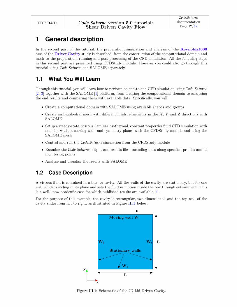
For the purpose of this example, the cavity is rectangular, two-dimensional, and the top wall of thecavity slides from left to right, as illustrated in Figure III.1 below.
Wb
Wl Wr
Moving wall Wt
Stationary walls
L
L
y
x
Figure III.1: Schematic of the 2D Lid Driven Cavity.
EDF R&D Code Saturne version 5.0 tutorial:Shear Driven Cavity Flow
Code SaturnedocumentationPage 13/47
Geometry
The cavity is a square of length L = 1.0 m.
Fluid Properties
The fluid is given the properties listed in Table III.1 below:
Property Value UnitsDensity (ρ) 1.0 kg/m3
Viscosity (µ) 10−3 Pa.s
Table III.1: Fluid Properties.
Boundary Conditions
The problem is considered to be isothermal and the domain is fully enclosed by impermeable, non-slipwalls. This means that, exactly at the surface of the walls, the fluid inside the box attaches to the wallsand has exactly the same velocity as the walls. Therefore, the problem is fully defined by specifyingthe velocity of the walls (Table III.2). The side and bottom walls are stationary. The top wall slidesin the positive X direction at a speed of 1.0 m.s−1.
Velocity component
Surface Vx (m/s) Vy (m/s)Wl 0.0 0.0Wb 0.0 0.0Wr 0.0 0.0Wt 1.0 0.0
Table III.2: Wall velocities.
Flow Regime
The flow Reynolds number is evaluated to determine whether the flow is in the laminar or turbulentregime. The Reynolds number is calculated based on the lid velocity, the box dimensions, and thefluid properties.
For this case, the fluid properties and lid velocity have been chosen so that Re = ρ·U ·Lµ = 1000,
indicating that the problem is in the laminar flow regime.
1.3 Creating the Code Saturne case
The DrivenCavity study and Reynolds1000 case are created by following the instructions in sectionII of this tutorial.
The next paragraphs describe how to setup and run the lid driven cavity simulations for a flow Reynoldsnumber of 1000.
2 Creating the Computational Domain within SALOMEFirst you need to create the geometry of the cavity which defines the bounds of the computationaldomain and then mesh this domain. Installation of this tool is described in section II.
EDF R&D Code Saturne version 5.0 tutorial:Shear Driven Cavity Flow
Code SaturnedocumentationPage 14/47
Code Saturne is a 3D code and, therefore, the computational domain will be created as a 3D box,aligned with the X, Y , and Z directions. However, as we are only interested in 2D modelling and theflow motion in the X−Y plane, the box will be designed to be thin and contain only one computationalcell in the Z direction.
2.1 Geometry
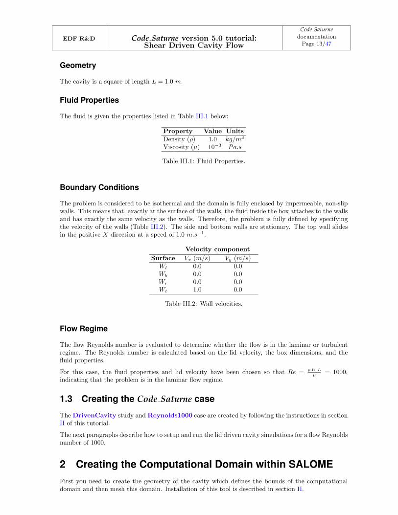
Once the CFD case structure is created from the CFDStudy module, the current SALOME file issaved by accessing File Save . For this tutorial, we choose the file name Cavity (Figure III.2). Thefile Cavity.hdf will be created in directory Driven Cavity.
Figure III.2: Saving the SALOME file
It is advisable to save the file at regular intervals when preparing a case, preferably, before and followingall significant modifications. That way your latest work is preserved and, should mistakes happen, itis always possible to exit SALOME and restart it from the latest saved file.
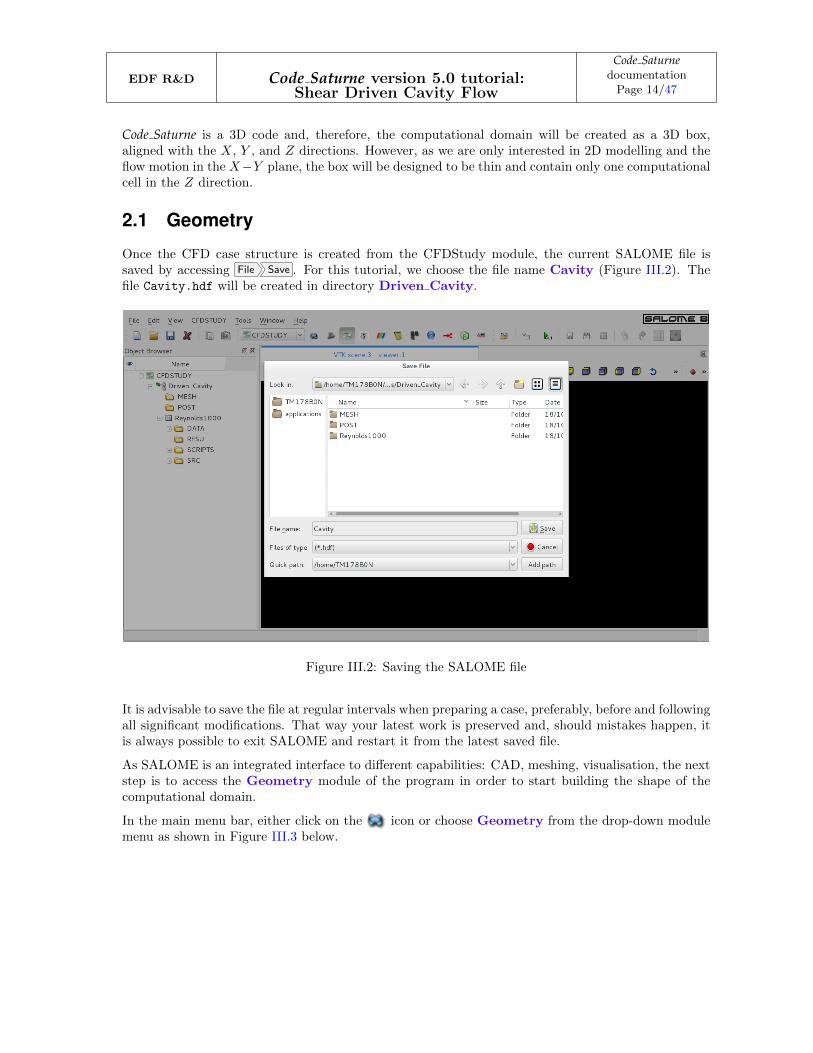
As SALOME is an integrated interface to different capabilities: CAD, meshing, visualisation, the nextstep is to access the Geometry module of the program in order to start building the shape of thecomputational domain.
In the main menu bar, either click on the icon or choose Geometry from the drop-down modulemenu as shown in Figure III.3 below.
EDF R&D Code Saturne version 5.0 tutorial:Shear Driven Cavity Flow
Code SaturnedocumentationPage 15/47
Figure III.3: Selecting Geometry in the module chooser.
The Geometry menus then become available in the top bar and the OCC scene viewer opens inthe right hand side, where the geometry objects can be visualised and manipulated. The scene viewercomes with its own set of 3D-viewing menus to control the display and perform operations such aspanning in and out, and rotating and moving the object in the scene.
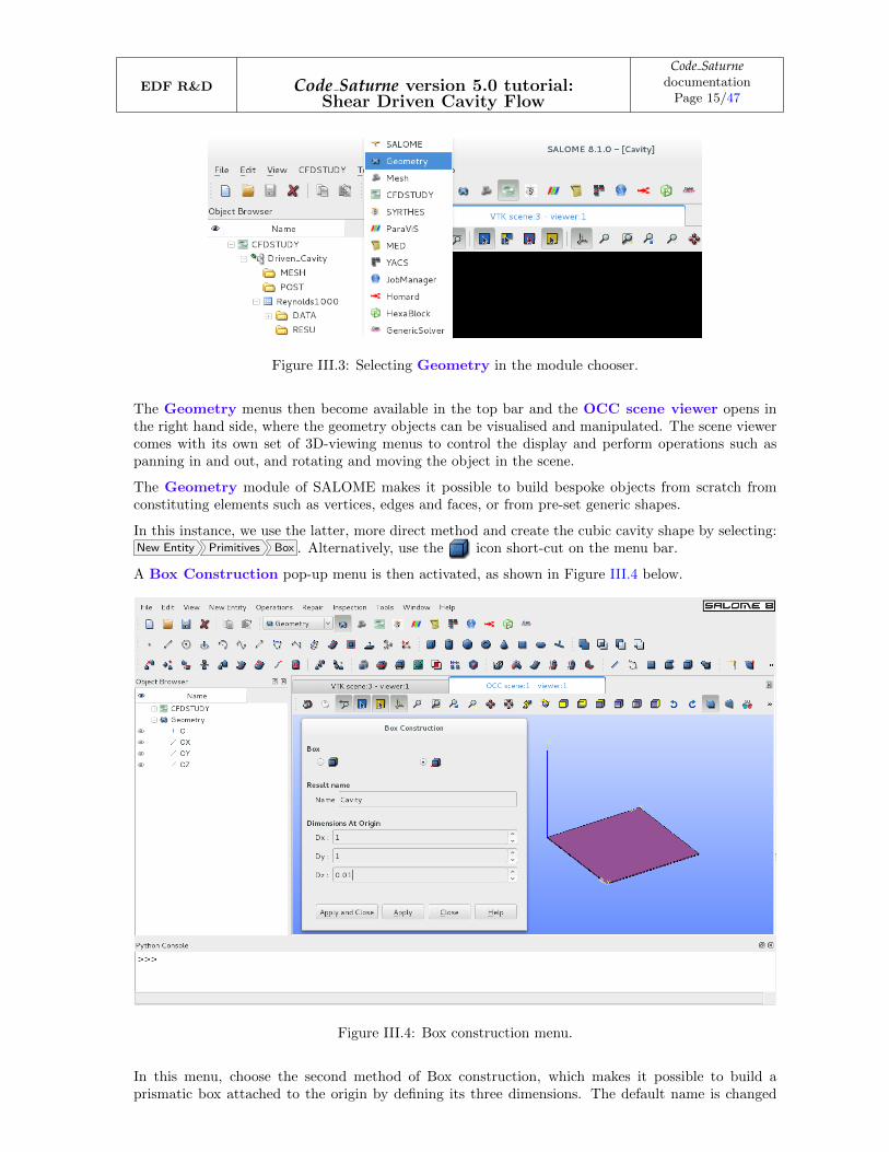
The Geometry module of SALOME makes it possible to build bespoke objects from scratch fromconstituting elements such as vertices, edges and faces, or from pre-set generic shapes.
In this instance, we use the latter, more direct method and create the cubic cavity shape by selecting:New Entity Primitives Box . Alternatively, use the icon short-cut on the menu bar.
A Box Construction pop-up menu is then activated, as shown in Figure III.4 below.
Figure III.4: Box construction menu.
In this menu, choose the second method of Box construction, which makes it possible to build aprismatic box attached to the origin by defining its three dimensions. The default name is changed
EDF R&D Code Saturne version 5.0 tutorial:Shear Driven Cavity Flow
Code SaturnedocumentationPage 16/47
to Cavity and the dimensions in the X, Y , and Z directions are specified according to the problemdefinition in paragraph 1.2.
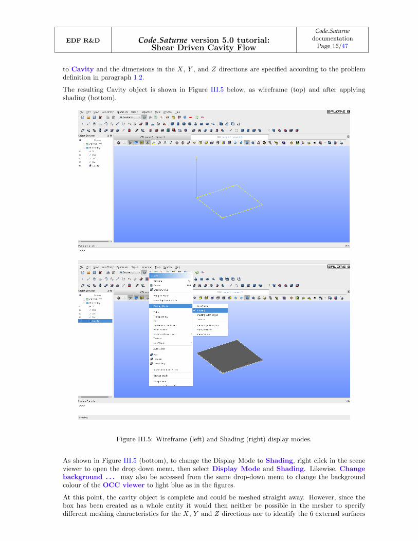
The resulting Cavity object is shown in Figure III.5 below, as wireframe (top) and after applyingshading (bottom).
Figure III.5: Wireframe (left) and Shading (right) display modes.
As shown in Figure III.5 (bottom), to change the Display Mode to Shading, right click in the sceneviewer to open the drop down menu, then select Display Mode and Shading. Likewise, Changebackground . . . may also be accessed from the same drop-down menu to change the backgroundcolour of the OCC viewer to light blue as in the figures.
At this point, the cavity object is complete and could be meshed straight away. However, since thebox has been created as a whole entity it would then neither be possible in the mesher to specifydifferent meshing characteristics for the X, Y and Z directions nor to identify the 6 external surfaces

EDF R&D Code Saturne version 5.0 tutorial:Shear Driven Cavity Flow
Code SaturnedocumentationPage 17/47
as boundaries for the Code Saturne calculations. Before meshing, it is then necessary to create andidentify these elements. In the next step, you will automatically create Edges Groups using thePropagate utility. Faces Groups will then be created by manually selecting them.
With the Cavity object selected in the Object Browser in the left-hand column, in the top menubar, click on Operations Blocks Propagate as shown in Figure III.6 below. By using the Apply and Close
action at the bottom of the menu, you will be able to automatically create three Edges Groups, eachof them containing every edges parallel to one direction.
Figure III.6: Using the Propagate utility to automatically create Edges Groups.
One can now rename them as X Edges, Y Edges and Z Edges by right-clicking on each group andthen select Rename. The Cavity object in the object browser should now contain three EdgesGroups as shown in Figure III.7 below.
EDF R&D Code Saturne version 5.0 tutorial:Shear Driven Cavity Flow
Code SaturnedocumentationPage 18/47
Figure III.7: Cavity with the X Edges, Y Edges and Z Edges groups.
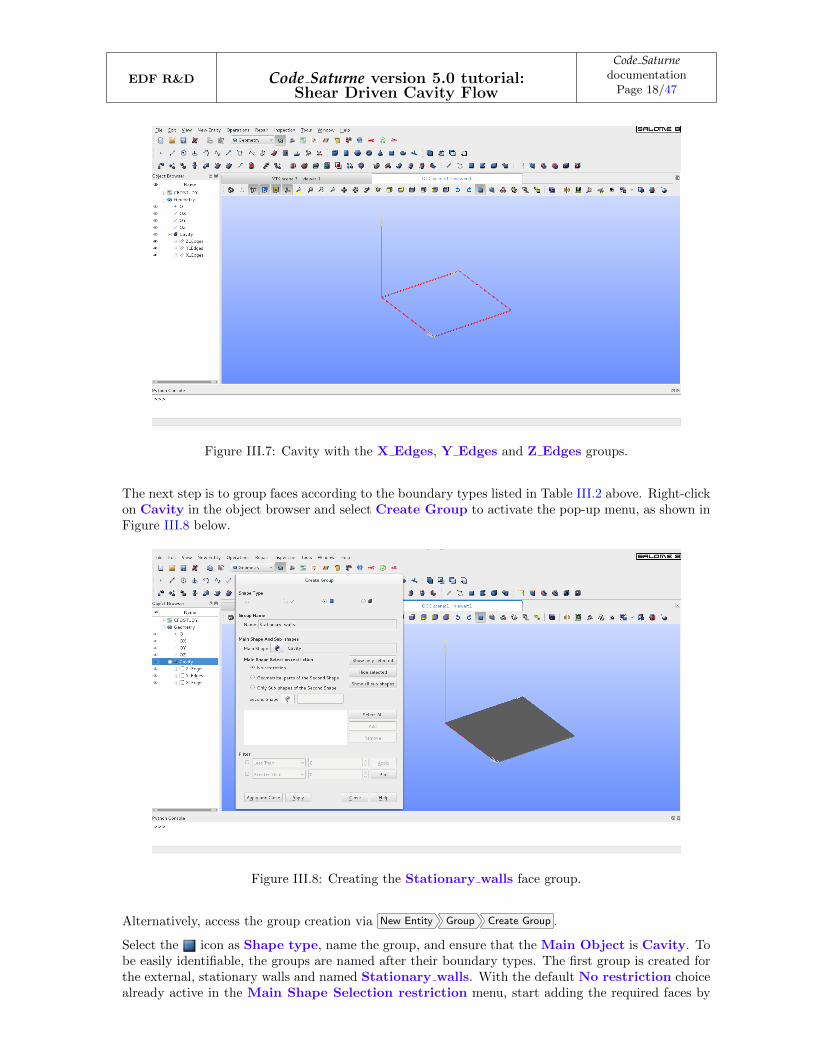
The next step is to group faces according to the boundary types listed in Table III.2 above. Right-clickon Cavity in the object browser and select Create Group to activate the pop-up menu, as shown inFigure III.8 below.
Figure III.8: Creating the Stationary walls face group.
Alternatively, access the group creation via New Entity Group Create Group .
Select the icon as Shape type, name the group, and ensure that the Main Object is Cavity. Tobe easily identifiable, the groups are named after their boundary types. The first group is created forthe external, stationary walls and named Stationary walls. With the default No restriction choicealready active in the Main Shape Selection restriction menu, start adding the required faces by

EDF R&D Code Saturne version 5.0 tutorial:Shear Driven Cavity Flow
Code SaturnedocumentationPage 19/47
left-clicking on them in the OCC viewer and then pressing Add . One can zoom with the mousewheel as well as rotate the Cavity object by holding Ctrl + Right Click to select the faces more easily.The faces may be added one by one, or together by multiple-selection through left-clicking and holdingthe Ctrl key. Once the three faces are selected, one can check them by pressing the Show only selected
button. The Create Group menu should look as shown in Figure III.9.
Figure III.9: Selected faces of the Stationary walls face group.
Press Apply and repeat these steps for the next two groups: Symmetry plane and Sliding wall,pressing Apply each time. Conclude the creation of face groups by pressing Apply and Close .
The face and edges groups are now listed under the Cavity object in the Object Browser (Figure III.10).
Figure III.10: Cavity with the edges, faces, and groups.
EDF R&D Code Saturne version 5.0 tutorial:Shear Driven Cavity Flow
Code SaturnedocumentationPage 20/47
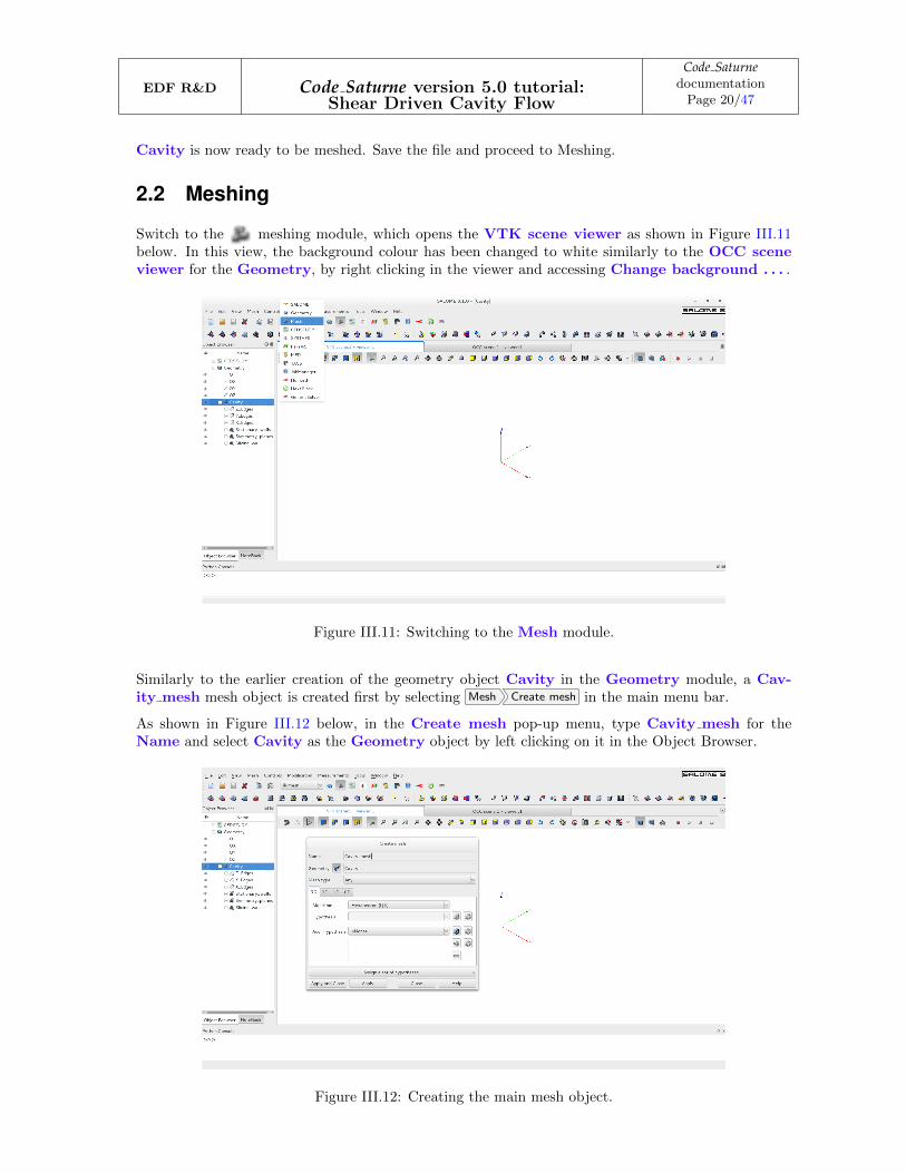
Cavity is now ready to be meshed. Save the file and proceed to Meshing.
2.2 Meshing
Switch to the meshing module, which opens the VTK scene viewer as shown in Figure III.11below. In this view, the background colour has been changed to white similarly to the OCC sceneviewer for the Geometry, by right clicking in the viewer and accessing Change background . . . .
Figure III.11: Switching to the Mesh module.
Similarly to the earlier creation of the geometry object Cavity in the Geometry module, a Cav-ity mesh mesh object is created first by selecting Mesh Create mesh in the main menu bar.
As shown in Figure III.12 below, in the Create mesh pop-up menu, type Cavity mesh for theName and select Cavity as the Geometry object by left clicking on it in the Object Browser.
Figure III.12: Creating the main mesh object.
EDF R&D Code Saturne version 5.0 tutorial:Shear Driven Cavity Flow
Code SaturnedocumentationPage 21/47
The main mesh object holds the global characteristics of the Cavity mesh.
For the volume, in the 3D tab choose Hexahedron (i,j,k). All the (external) surfaces of the Cavitywill be meshed similarly, therefore a global setup is applied for the entire mesh via this pop-up menuby clicking on the 2D tab and selecting Quadrangle: Mapping. These two selections will result in ablock-structured mesh, with an (i, j, k) matrix structure. This requires identical discretisations alongall the edges aligned along the same directions. If we wanted the discretisation to be the same alongall the directions, for example 15 sub-divisions along the X, Y , and Z edges, the 1D tab could beselected and this unique discretisation specified. However, here we need to be able, at least, to specifythe Z direction independently of the two others to create a 3D domain which is only one cell deep.Therefore, the edge discretisations will be specified separately using sub-meshes.
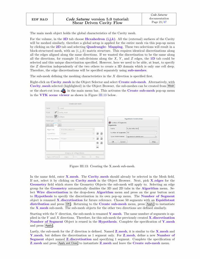
The sub-mesh defining the meshing characteristics in the X direction is specified first.
Right-click on Cavity mesh in the Object Selector and select Create sub-mesh. Alternatively, withCavity mesh selected (highlighted) in the Object Browser, the sub-meshes can be created from Mesh
or the short-cut icon in the main menu bar. This activates the Create sub-mesh pop-up menu
in the VTK scene viewer as shown in Figure III.13 below.
Figure III.13: Creating the X mesh sub-mesh.
In the name field, enter X mesh. The Cavity mesh should already be selected in the Mesh field.If not, select it by clicking on Cavity mesh in the Object Browser. Next, pick X edges for theGeometry field which stores the Geometry Objects the sub-mesh will apply to. Selecting an edgegroup for the Geometry automatically disables the 3D and 2D tabs in the Algorithm menu. Se-lect Wire discretisation in the drop-down Algorithm menu and press on the gear button nextto Hypothesis to specify the discretisation in its own pop-up menu. The Number of Segmentobject is renamed X discretisation for future reference. Choose 50 segments with an Equidistantdistribution and press OK . Returning to the Create sub-mesh menu, press Apply to instantiatethe X mesh sub-mesh. The sub-mesh objects for the other two directions are defined similarly.
Starting with the Y direction, the sub-mesh is renamed Y mesh. The same number of segments is ap-plied in the Y and X directions. Therefore, for this sub-mesh the previously created X discretisationNumber of Segment Object is reused in the Hypothesis. Complete the specification of Y meshand press Apply .
Lastly, the sub-mesh for the Z direction is defined. Named Z mesh, it is similar to the X mesh andY mesh, but defines the discretisation as 1 segment only. For Z mesh, define a new Number ofSegment object named Z discretisation and specifying 1 segment. Complete the specification ofZ mesh and press Apply and Close to instantiate Z mesh and leave the Create sub-mesh menu.
EDF R&D Code Saturne version 5.0 tutorial:Shear Driven Cavity Flow
Code SaturnedocumentationPage 22/47
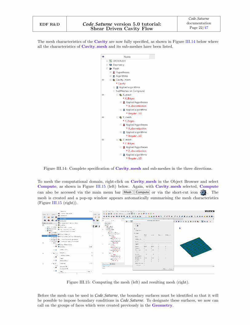
The mesh characteristics of the Cavity are now fully specified, as shown in Figure III.14 below whereall the characteristics of Cavity mesh and its sub-meshes have been listed.
Figure III.14: Complete specification of Cavity mesh and sub-meshes in the three directions.
To mesh the computational domain, right-click on Cavity mesh in the Object Browser and selectCompute, as shown in Figure III.15 (left) below. Again, with Cavity mesh selected, Compute
can also be accessed via the main menu bar Mesh Compute or via the short-cut icon . The
mesh is created and a pop-up window appears automatically summarising the mesh characteristics(Figure III.15 (right)).
Figure III.15: Computing the mesh (left) and resulting mesh (right).
Before the mesh can be used in Code Saturne, the boundary surfaces must be identified so that it willbe possible to impose boundary conditions in Code Saturne. To designate these surfaces, we now cancall on the groups of faces which were created previously in the Geometry.
EDF R&D Code Saturne version 5.0 tutorial:Shear Driven Cavity Flow
Code SaturnedocumentationPage 23/47
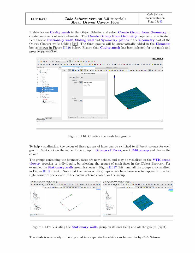
Right-click on Cavity mesh in the Object Selector and select Create Group from Geometry tocreate containers of mesh elements. The Create Group from Geometry pop-menu is activated.Left click on Stationary walls, Sliding wall and Symmetry planes in the Geometry part of theObject Chooser while holding . The three groups will be automatically added in the Elementsbox as shown in Figure III.16 below. Ensure that Cavity mesh has been selected for the mesh andpress Apply and Close .
Figure III.16: Creating the mesh face groups.
To help visualisation, the colour of these groups of faces can be switched to different colours for eachgroup. Right click on the name of the group in Groups of Faces, select Edit group and choose thecolour.
The groups containing the boundary faces are now defined and may be visualised in the VTK sceneviewer, together or individually, by selecting the groups of mesh faces in the Object Browser. Forexample, the Stationary walls group is shown in Figure III.17 (left), and all the groups are visualisedin Figure III.17 (right). Note that the names of the groups which have been selected appear in the topright corner of the viewer, in the colour scheme chosen for the group.
Figure III.17: Visualing the Stationary walls group on its own (left) and all the groups (right).
The mesh is now ready to be exported in a separate file which can be read in by Code Saturne.

EDF R&D Code Saturne version 5.0 tutorial:Shear Driven Cavity Flow
Code SaturnedocumentationPage 24/47
Before exporting the file, it is important to highlight an important naming convention, as the namesof the mesh and its elements will be used as their identifiers in Code Saturne.
Save the SALOME file and export the mesh file in .med format by selecting from the main menu: File
Export MED file , as shown in Figure III.18 below. The file should be placed in the MESH directoryof the DrivenCavity study, where Code Saturne will expect the file to be situated by default.
Figure III.18: Exporting the mesh file in .med format.
For the file name, choose Cavity mesh; the .med extension is automatically added. You are nowready to set up the CFD simulation with the CFDStudy module.
3 Simulating within SALOME
3.1 Setting up the CFD Simulation
To set-up the CFD Simulation, select the CFDStudy module by clicking on the CFDStudy button orby selecting CFDStudy in the modules drop-down menu as shown in Figure III.19.
Figure III.19: Selecting the CFDStudy module.
Then, right click on Reynolds1000 in the Object Browser and launch the Code Saturne GUI inside
EDF R&D Code Saturne version 5.0 tutorial:Shear Driven Cavity Flow
Code SaturnedocumentationPage 25/47
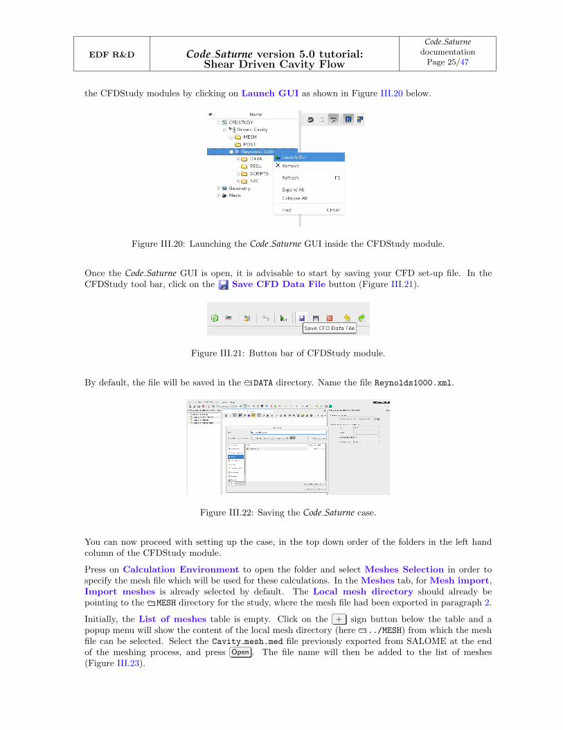
the CFDStudy modules by clicking on Launch GUI as shown in Figure III.20 below.
Figure III.20: Launching the Code Saturne GUI inside the CFDStudy module.
Once the Code Saturne GUI is open, it is advisable to start by saving your CFD set-up file. In theCFDStudy tool bar, click on the Save CFD Data File button (Figure III.21).
Figure III.21: Button bar of CFDStudy module.
By default, the file will be saved in the DATA directory. Name the file Reynolds1000.xml.
Figure III.22: Saving the Code Saturne case.
You can now proceed with setting up the case, in the top down order of the folders in the left handcolumn of the CFDStudy module.
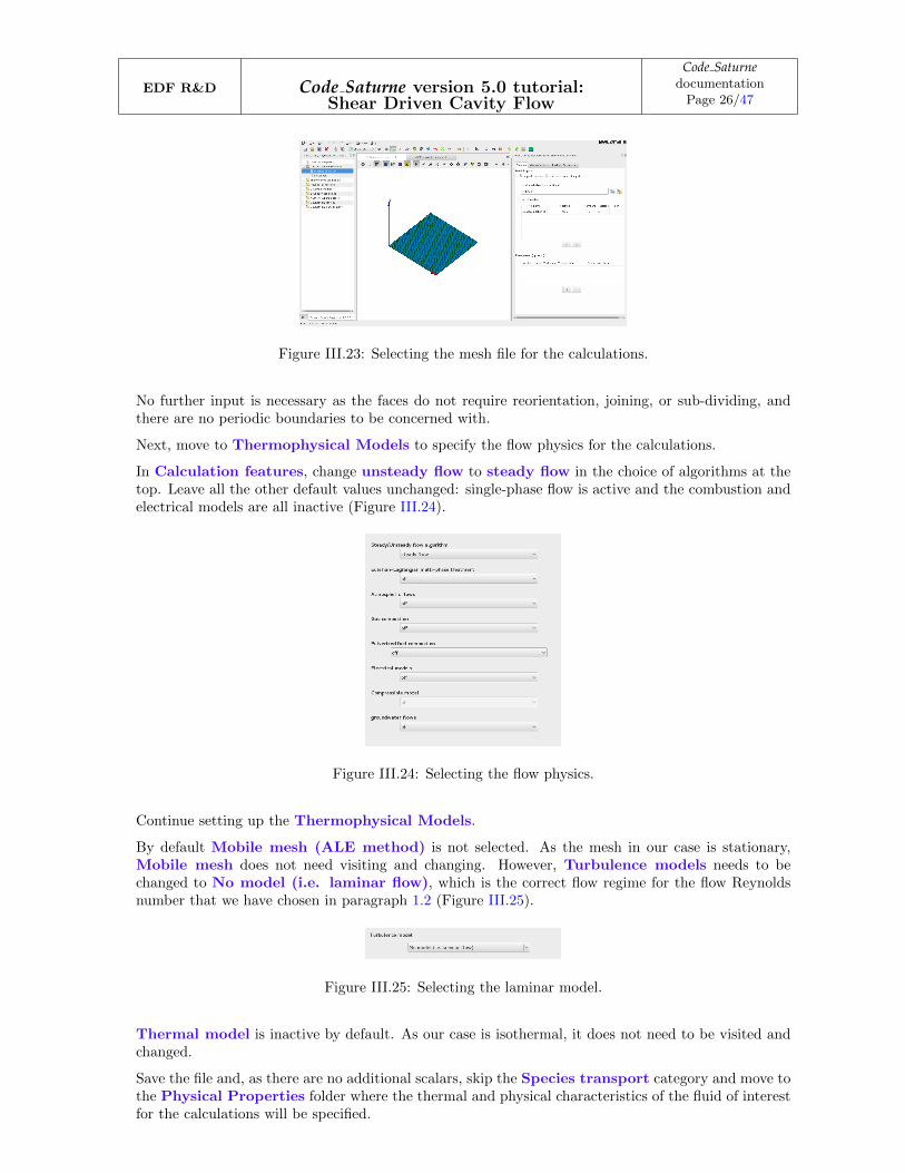
Press on Calculation Environment to open the folder and select Meshes Selection in order tospecify the mesh file which will be used for these calculations. In the Meshes tab, for Mesh import,Import meshes is already selected by default. The Local mesh directory should already bepointing to the MESH directory for the study, where the mesh file had been exported in paragraph 2.
Initially, the List of meshes table is empty. Click on the + sign button below the table and apopup menu will show the content of the local mesh directory (here ../MESH) from which the meshfile can be selected. Select the Cavity mesh.med file previously exported from SALOME at the endof the meshing process, and press Open . The file name will then be added to the list of meshes(Figure III.23).
EDF R&D Code Saturne version 5.0 tutorial:Shear Driven Cavity Flow
Code SaturnedocumentationPage 26/47
Figure III.23: Selecting the mesh file for the calculations.
No further input is necessary as the faces do not require reorientation, joining, or sub-dividing, andthere are no periodic boundaries to be concerned with.
Next, move to Thermophysical Models to specify the flow physics for the calculations.
In Calculation features, change unsteady flow to steady flow in the choice of algorithms at thetop. Leave all the other default values unchanged: single-phase flow is active and the combustion andelectrical models are all inactive (Figure III.24).
Figure III.24: Selecting the flow physics.
Continue setting up the Thermophysical Models.
By default Mobile mesh (ALE method) is not selected. As the mesh in our case is stationary,Mobile mesh does not need visiting and changing. However, Turbulence models needs to bechanged to No model (i.e. laminar flow), which is the correct flow regime for the flow Reynoldsnumber that we have chosen in paragraph 1.2 (Figure III.25).
Figure III.25: Selecting the laminar model.
Thermal model is inactive by default. As our case is isothermal, it does not need to be visited andchanged.
Save the file and, as there are no additional scalars, skip the Species transport category and move tothe Physical Properties folder where the thermal and physical characteristics of the fluid of interestfor the calculations will be specified.
EDF R&D Code Saturne version 5.0 tutorial:Shear Driven Cavity Flow
Code SaturnedocumentationPage 27/47
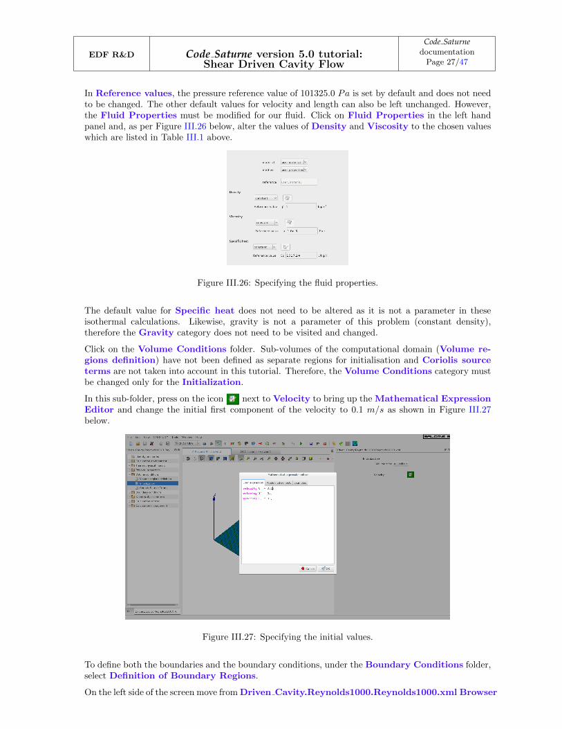
In Reference values, the pressure reference value of 101325.0 Pa is set by default and does not needto be changed. The other default values for velocity and length can also be left unchanged. However,the Fluid Properties must be modified for our fluid. Click on Fluid Properties in the left handpanel and, as per Figure III.26 below, alter the values of Density and Viscosity to the chosen valueswhich are listed in Table III.1 above.
Figure III.26: Specifying the fluid properties.
The default value for Specific heat does not need to be altered as it is not a parameter in theseisothermal calculations. Likewise, gravity is not a parameter of this problem (constant density),therefore the Gravity category does not need to be visited and changed.
Click on the Volume Conditions folder. Sub-volumes of the computational domain (Volume re-gions definition) have not been defined as separate regions for initialisation and Coriolis sourceterms are not taken into account in this tutorial. Therefore, the Volume Conditions category mustbe changed only for the Initialization.
In this sub-folder, press on the icon next to Velocity to bring up the Mathematical ExpressionEditor and change the initial first component of the velocity to 0.1 m/s as shown in Figure III.27below.
Figure III.27: Specifying the initial values.
To define both the boundaries and the boundary conditions, under the Boundary Conditions folder,select Definition of Boundary Regions.
On the left side of the screen move from Driven Cavity.Reynolds1000.Reynolds1000.xml Browser
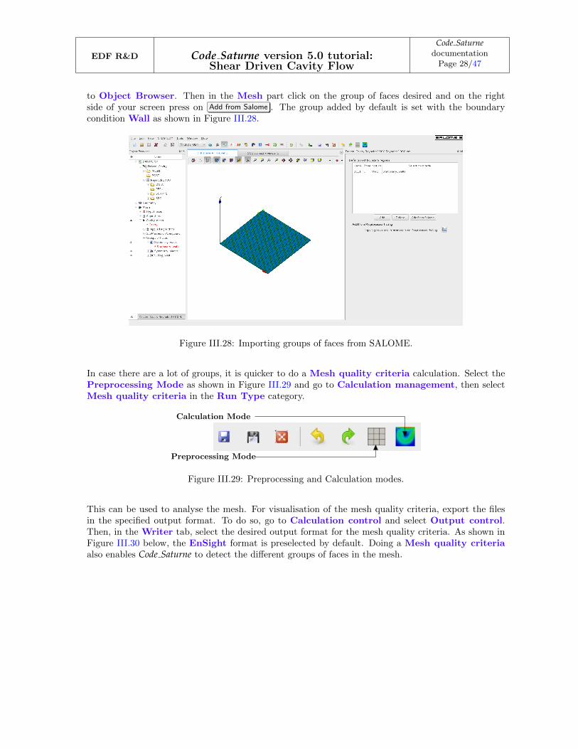
EDF R&D Code Saturne version 5.0 tutorial:Shear Driven Cavity Flow
Code SaturnedocumentationPage 28/47
to Object Browser. Then in the Mesh part click on the group of faces desired and on the rightside of your screen press on Add from Salome . The group added by default is set with the boundarycondition Wall as shown in Figure III.28.
Figure III.28: Importing groups of faces from SALOME.
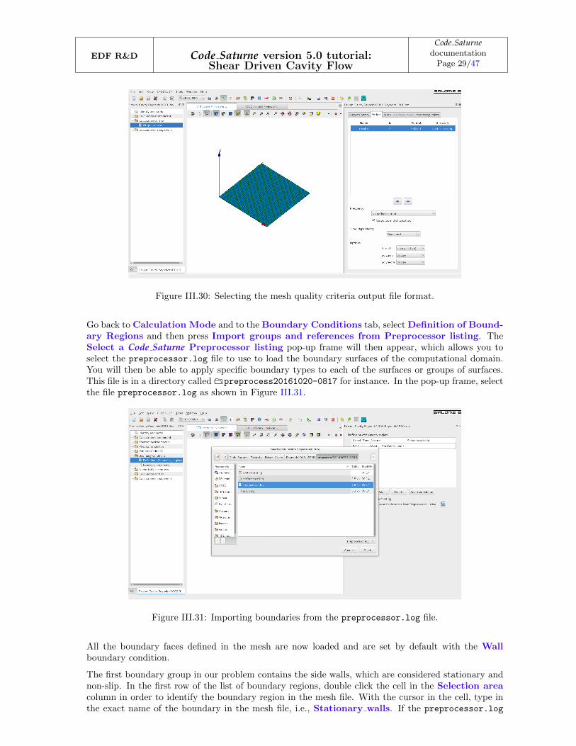
In case there are a lot of groups, it is quicker to do a Mesh quality criteria calculation. Select thePreprocessing Mode as shown in Figure III.29 and go to Calculation management, then selectMesh quality criteria in the Run Type category.
Preprocessing Mode
Calculation Mode
Figure III.29: Preprocessing and Calculation modes.
This can be used to analyse the mesh. For visualisation of the mesh quality criteria, export the filesin the specified output format. To do so, go to Calculation control and select Output control.Then, in the Writer tab, select the desired output format for the mesh quality criteria. As shown inFigure III.30 below, the EnSight format is preselected by default. Doing a Mesh quality criteriaalso enables Code Saturne to detect the different groups of faces in the mesh.
EDF R&D Code Saturne version 5.0 tutorial:Shear Driven Cavity Flow
Code SaturnedocumentationPage 29/47
Figure III.30: Selecting the mesh quality criteria output file format.
Go back to Calculation Mode and to the Boundary Conditions tab, select Definition of Bound-ary Regions and then press Import groups and references from Preprocessor listing. TheSelect a Code Saturne Preprocessor listing pop-up frame will then appear, which allows you toselect the preprocessor.log file to use to load the boundary surfaces of the computational domain.You will then be able to apply specific boundary types to each of the surfaces or groups of surfaces.This file is in a directory called preprocess20161020-0817 for instance. In the pop-up frame, selectthe file preprocessor.log as shown in Figure III.31.
Figure III.31: Importing boundaries from the preprocessor.log file.
All the boundary faces defined in the mesh are now loaded and are set by default with the Wallboundary condition.
The first boundary group in our problem contains the side walls, which are considered stationary andnon-slip. In the first row of the list of boundary regions, double click the cell in the Selection areacolumn in order to identify the boundary region in the mesh file. With the cursor in the cell, type inthe exact name of the boundary in the mesh file, i.e., Stationary walls. If the preprocessor.log
EDF R&D Code Saturne version 5.0 tutorial:Shear Driven Cavity Flow
Code SaturnedocumentationPage 30/47
file has been used, the Selection area is already completed.
The second set of boundaries are the symmetry planes which are used to enforce the 2D nature of theproblem. In the second row, double click on Wall in the Nature column to activate the drop downmenu ofboundary types. Choose Symmetry and release the menu. In the Selection criteria cell,input the name of the boundary in the mesh file, i.e.,Symmetry planes, if no preprocessor.log filehas been used.
In the third row of the table, as for the two other boundary conditions, input the name of the slidingwall boundary in the mesh file, i.e., Sliding wall if no preprocessor.log file has been used.
Note that it is better to press enter after typing in the name of the region to ensure that it is properlyrecorded by the GUI.
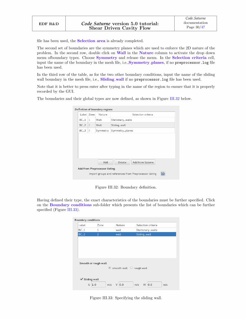
The boundaries and their global types are now defined, as shown in Figure III.32 below.
Figure III.32: Boundary definition.
Having defined their type, the exact characteristics of the boundaries must be further specified. Clickon the Boundary conditions sub-folder which presents the list of boundaries which can be furtherspecified (Figure III.33).
Figure III.33: Specifying the sliding wall.
EDF R&D Code Saturne version 5.0 tutorial:Shear Driven Cavity Flow
Code SaturnedocumentationPage 31/47
The symmetry boundaries are fully defined and do not need further specification. Therefore, they donot appear in the list. However, Wall boundaries can each be further defined as smooth or rough,and as Sliding wall. By default, the wall surface is smooth and this parameter does not need tobe changed. The Stationary walls boundary is fixed and fully specified. However, click on theSliding wall boundary and activate the Sliding wall selection. Fields then appear for the U, V,and W velocity components of the wall. By default, these velocities are null. Click in the U field andenter 1.0, as shown in Figure III.33.
The mesh and physics of the problem have now been set up. Now, parameters related to the calculationcan be specified.
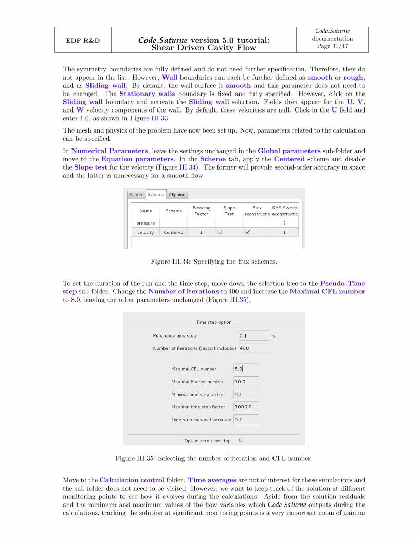
In Numerical Parameters, leave the settings unchanged in the Global parameters sub-folder andmove to the Equation parameters. In the Scheme tab, apply the Centered scheme and disablethe Slope test for the velocity (Figure III.34). The former will provide second-order accuracy in spaceand the latter is unnecessary for a smooth flow.
Figure III.34: Specifying the flux schemes.
To set the duration of the run and the time step, move down the selection tree to the Pseudo-Timestep sub-folder. Change the Number of iterations to 400 and increase the Maximal CFL numberto 8.0, leaving the other parameters unchanged (Figure III.35).
Figure III.35: Selecting the number of iteration and CFL number.
Move to the Calculation control folder. Time averages are not of interest for these simulations andthe sub-folder does not need to be visited. However, we want to keep track of the solution at differentmonitoring points to see how it evolves during the calculations. Aside from the solution residualsand the minimum and maximum values of the flow variables which Code Saturne outputs during thecalculations, tracking the solution at significant monitoring points is a very important mean of gaining
EDF R&D Code Saturne version 5.0 tutorial:Shear Driven Cavity Flow
Code SaturnedocumentationPage 32/47
confidence in the convergence of the calculations and judging whether calculations have been run fora sufficiently large number of iterations. This is explained further in paragraph 3.2 below.
Click on the Output control sub-folder panel. The first three tabs, Output control, Writer, andMesh are set by default to the correct values for this case and do not need to be changed. TheLog frequency in the Output control tab is set to print the calculations diagnostics such as theresiduals at each time step. In the Writer tab, the format of the results file which will be used for post-processing is already set to EnSight, which is compatible with the SALOME module ParaVis whichwill be used to post-process the results after the run. The file will be located in the postprocessing
sub-directory of Reynolds1000/RESU/runDateAndTime, where runDateAndTime corresponds to thetime at which the run was started. Clicking on the results row brings up the additional informationabout the Frequency, Time-dependency and Options. As already set by default, the results filewill only be written at the end of the run and on the Fixed mesh used for this case. The Optionsrelate to the specific details of the file format. The Mesh tab is already set to output the calculationsdata in all the fluids cells and at all boundary faces to the results file.
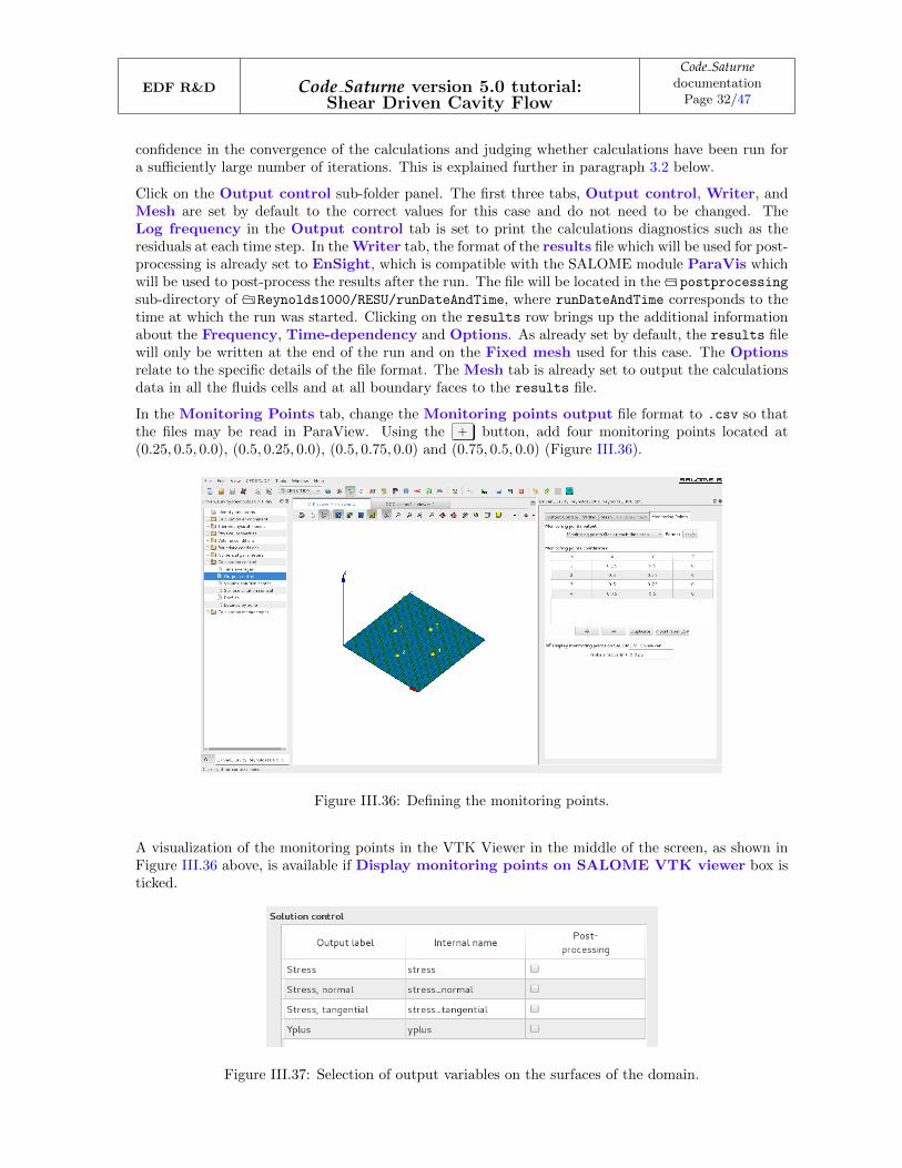
In the Monitoring Points tab, change the Monitoring points output file format to .csv so thatthe files may be read in ParaView. Using the + button, add four monitoring points located at(0.25, 0.5, 0.0), (0.5, 0.25, 0.0), (0.5, 0.75, 0.0) and (0.75, 0.5, 0.0) (Figure III.36).
Figure III.36: Defining the monitoring points.
A visualization of the monitoring points in the VTK Viewer in the middle of the screen, as shown inFigure III.36 above, is available if Display monitoring points on SALOME VTK viewer box isticked.
Figure III.37: Selection of output variables on the surfaces of the domain.

EDF R&D Code Saturne version 5.0 tutorial:Shear Driven Cavity Flow
Code SaturnedocumentationPage 33/47
Click on the Surface solution control sub-folder and disable Post-processing for Yplus and Stressas they are not relevant to these simulations (Figure III.37).
Lastly, we want to output one-dimensional profiles of variables along straight lines at the end of thecalculations. Click on Profiles and add two profiles which go through the centre of the Cavity byclicking on the Add button. The first one for the X velocity along the Y axis and the second one forthe Y velocity along the X axis. In turn, specify all the fields listed below the table of profiles, startingwith Filename and finishing with the variables which are to be stored on output.
For the X velocity profile, choose XVel YaxisCenterLine for Filename, and .csv for Formatso that the profiles may be read in the ParaVis post-processing module of SALOME. The Outputfrequency must be set to at the end of the calculation. To define the line, press on the Math-ematical expression editor button adjacent to Line Definition. The line is defined by thefollowing equation :
x = 0.5y = sz = 0.0
By definition, s varies between 0 and 1.0. For the Number of points enter 50 to account for the 50cells across the domain’s height. Finally, click on Velocity[0] and use the button to add it in thelist of variables, and press Add to store the profile in the list (Figure III.38).
Figure III.38: Specifying the 1D output profiles.
Repeat the procedure for the Y-velocity profiles, this time entering YVel XaxisCenterLine for File-name, and the following equation for the line defition :
x = sy = 0.5z = 0.0
Select the Velocity[1] variable instead of Velocity[0]. The Reynolds1000 case CFD simulation isnow ready to run.
In the folder Calculation management, go directly to the Prepare batch calculation sub-folder.By default, the calculation-restart is disabled in Start/Restart and so this sub-folder does not need

EDF R&D Code Saturne version 5.0 tutorial:Shear Driven Cavity Flow
Code SaturnedocumentationPage 34/47
to be visited. In the Prepare batch calculation sub-folder panel (Figure III.39), select the script filewhich is by default runcase by clicking on the folder button . A pop-up window opens up, select
the runcase file and click on Open . For the Run type, select Standard (calculations without meshor partitions import or pre-processing) and choose 1 processor for the Number of processes. Leavethe Run id and Threads per task to their default value.
Figure III.39: Batch calculation settings.
Press the Start calculation button to run Code Saturne.
3.2 Running and Analysing the Simulation
Upon firing the Code Saturne run from the GUI, confirmation that Code Saturne is running, “Code Saturneis running”, appears in the window from which the GUI was started. This is followed by furthermessages indicating what stage the calculation is in, from “Preparing calculation data” to “Savingcalculation results”.
Wait for the calculations to complete and enter the Reynolds1000/RESU directory or open its con-tents via a browser to inspect its contents. Explanations of the meaning and purpose of the differentoutput files and directories resulting from a run are available in the Code Saturne Users Guide [3] andare not repeated here. Instead, we highlight individual items which relate to this specific run and howthe output information should always be used in order to analyse a calculation.
The RESU directory now contains a new directory named after the date and time at which thecalculation was started, expressed on a 24 hours clock in the format “YearMonthDay-HourMinutes”.
In this latter directory, notice in particular:
• The profile files XVel YaxisCenterLine and YVel XaxisCenterLine, written in .csv format,
• The listing file,
• The monitoring and postprocessing directories.
With your text editor, open one of the profile files, to inspect its structure. The requested variableslisted in column format as a function of the (x, y, z) coordinates of the points along the profile linedefined in the GUI.
EDF R&D Code Saturne version 5.0 tutorial:Shear Driven Cavity Flow
Code SaturnedocumentationPage 35/47
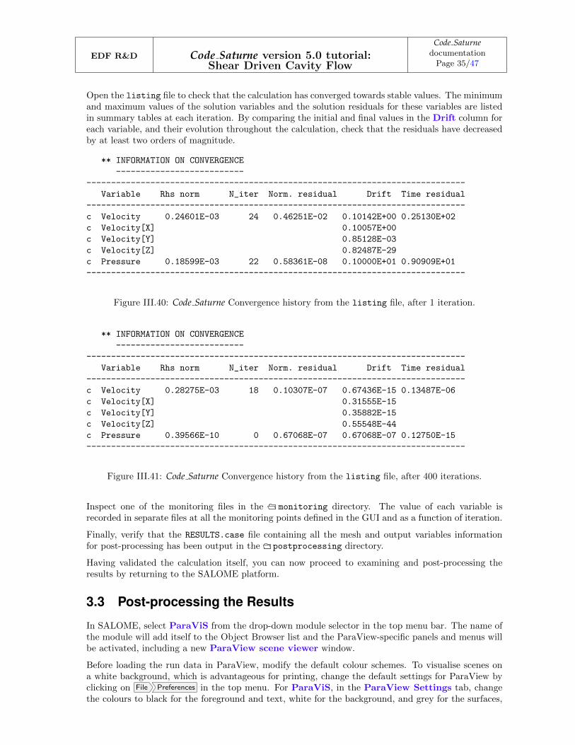
Open the listing file to check that the calculation has converged towards stable values. The minimumand maximum values of the solution variables and the solution residuals for these variables are listedin summary tables at each iteration. By comparing the initial and final values in the Drift column foreach variable, and their evolution throughout the calculation, check that the residuals have decreasedby at least two orders of magnitude.
** INFORMATION ON CONVERGENCE
--------------------------
-----------------------------------------------------------------------------
Variable Rhs norm N_iter Norm. residual Drift Time residual
-----------------------------------------------------------------------------
c Velocity 0.24601E-03 24 0.46251E-02 0.10142E+00 0.25130E+02
c Velocity[X] 0.10057E+00
c Velocity[Y] 0.85128E-03
c Velocity[Z] 0.82487E-29
c Pressure 0.18599E-03 22 0.58361E-08 0.10000E+01 0.90909E+01
-----------------------------------------------------------------------------
Figure III.40: Code Saturne Convergence history from the listing file, after 1 iteration.
** INFORMATION ON CONVERGENCE
--------------------------
-----------------------------------------------------------------------------
Variable Rhs norm N_iter Norm. residual Drift Time residual
-----------------------------------------------------------------------------
c Velocity 0.28275E-03 18 0.10307E-07 0.67436E-15 0.13487E-06
c Velocity[X] 0.31555E-15
c Velocity[Y] 0.35882E-15
c Velocity[Z] 0.55548E-44
c Pressure 0.39566E-10 0 0.67068E-07 0.67068E-07 0.12750E-15
-----------------------------------------------------------------------------
Figure III.41: Code Saturne Convergence history from the listing file, after 400 iterations.
Inspect one of the monitoring files in the monitoring directory. The value of each variable isrecorded in separate files at all the monitoring points defined in the GUI and as a function of iteration.
Finally, verify that the RESULTS.case file containing all the mesh and output variables informationfor post-processing has been output in the postprocessing directory.
Having validated the calculation itself, you can now proceed to examining and post-processing theresults by returning to the SALOME platform.
3.3 Post-processing the Results
In SALOME, select ParaViS from the drop-down module selector in the top menu bar. The name ofthe module will add itself to the Object Browser list and the ParaView-specific panels and menus willbe activated, including a new ParaView scene viewer window.
Before loading the run data in ParaView, modify the default colour schemes. To visualise scenes ona white background, which is advantageous for printing, change the default settings for ParaView byclicking on File Preferences in the top menu. For ParaViS, in the ParaView Settings tab, changethe colours to black for the foreground and text, white for the background, and grey for the surfaces,

EDF R&D Code Saturne version 5.0 tutorial:Shear Driven Cavity Flow
Code SaturnedocumentationPage 36/47
as shown in Figure III.42 below. Press Apply to enforce the new settings and OK to validate yourselection when you are satisfied with the changes.
Figure III.42: Setting the colour preferences for ParaView.
The data to post-process can now be imported in ParaView.
First, you are going to load the monitoring point data to validate that a stable, steady-state solutionhas been obtained. From the top menu bar, select File Open ParaView File . In the Open File poppanel, navigate to the monitoring sub-directory and select three files. The multiple selectionis performed by holding the Ctrl key down as you select the files. Select probes Pressure.csv,probes Velocity[X].csv, and probes Velocity[Y].csv. Close the panel by clicking OK . Thethree sets of data are now displayed under their file name in the Pipeline Browser. For each file,press Apply to load the data. By default, the data is visualised in tabular form in the ParaView scene
viewer. Close the View by clicking the cross button at the top, right hand corner of the view.
Then, click on the button to replace the data view by a Create View menu (Figure III.43).
EDF R&D Code Saturne version 5.0 tutorial:Shear Driven Cavity Flow
Code SaturnedocumentationPage 37/47
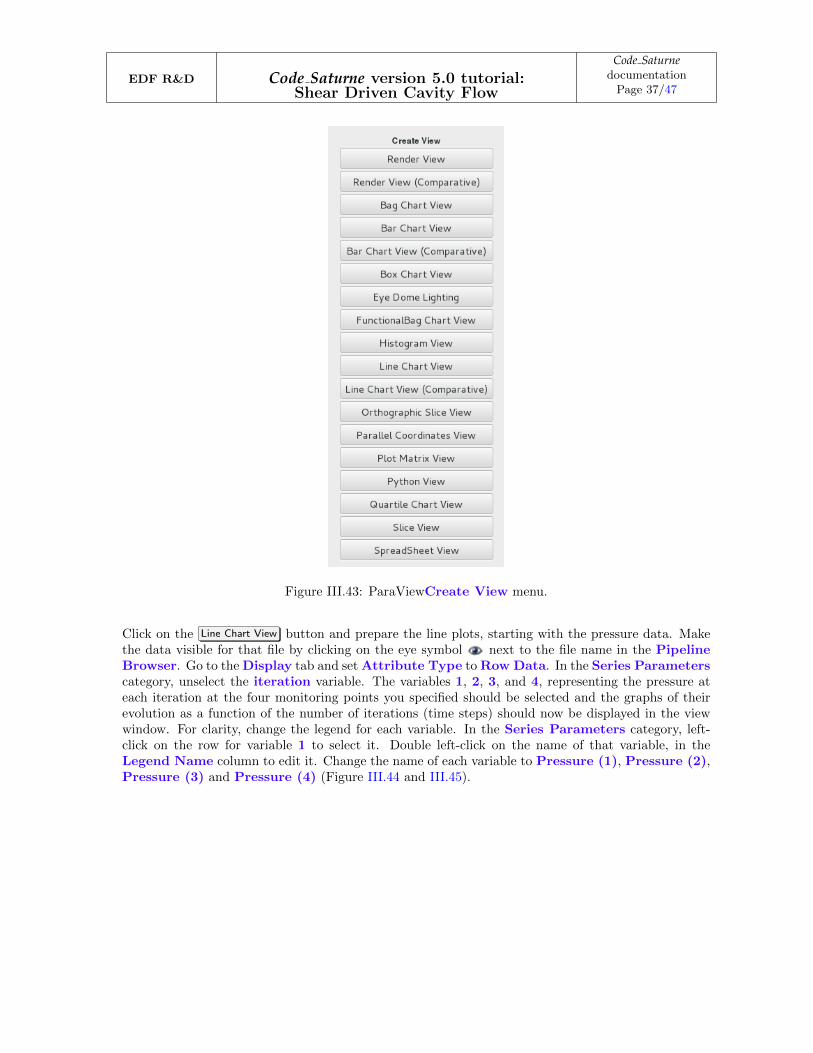
Figure III.43: ParaViewCreate View menu.
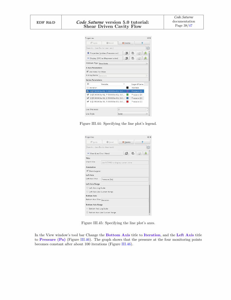
Click on the Line Chart View button and prepare the line plots, starting with the pressure data. Makethe data visible for that file by clicking on the eye symbol next to the file name in the PipelineBrowser. Go to the Display tab and set Attribute Type to Row Data. In the Series Parameterscategory, unselect the iteration variable. The variables 1, 2, 3, and 4, representing the pressure ateach iteration at the four monitoring points you specified should be selected and the graphs of theirevolution as a function of the number of iterations (time steps) should now be displayed in the viewwindow. For clarity, change the legend for each variable. In the Series Parameters category, left-click on the row for variable 1 to select it. Double left-click on the name of that variable, in theLegend Name column to edit it. Change the name of each variable to Pressure (1), Pressure (2),Pressure (3) and Pressure (4) (Figure III.44 and III.45).
EDF R&D Code Saturne version 5.0 tutorial:Shear Driven Cavity Flow
Code SaturnedocumentationPage 38/47
Figure III.44: Specifying the line plot’s legend.
Figure III.45: Specifying the line plot’s axes.
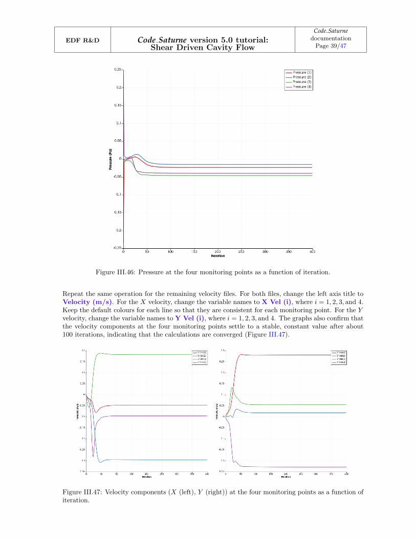
In the View window’s tool bar Change the Bottom Axis title to Iteration, and the Left Axis titleto Pressure (Pa) (Figure III.46). The graph shows that the pressure at the four monitoring pointsbecomes constant after about 100 iterations (Figure III.46).
EDF R&D Code Saturne version 5.0 tutorial:Shear Driven Cavity Flow
Code SaturnedocumentationPage 39/47
Figure III.46: Pressure at the four monitoring points as a function of iteration.
Repeat the same operation for the remaining velocity files. For both files, change the left axis title toVelocity (m/s). For the X velocity, change the variable names to X Vel (i), where i = 1, 2, 3, and 4.Keep the default colours for each line so that they are consistent for each monitoring point. For the Yvelocity, change the variable names to Y Vel (i), where i = 1, 2, 3, and 4. The graphs also confirm thatthe velocity components at the four monitoring points settle to a stable, constant value after about100 iterations, indicating that the calculations are converged (Figure III.47).
Figure III.47: Velocity components (X (left), Y (right)) at the four monitoring points as a function ofiteration.
EDF R&D Code Saturne version 5.0 tutorial:Shear Driven Cavity Flow
Code SaturnedocumentationPage 40/47
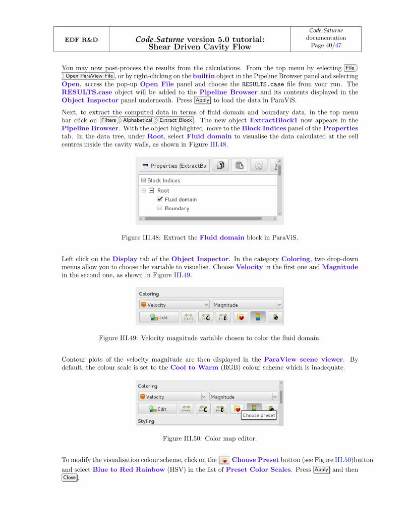
You may now post-process the results from the calculations. From the top menu by selecting File
Open ParaView File , or by right-clicking on the builtin object in the Pipeline Browser panel and selectingOpen, access the pop-up Open File panel and choose the RESULTS.case file from your run. TheRESULTS.case object will be added to the Pipeline Browser and its contents displayed in theObject Inspector panel underneath. Press Apply to load the data in ParaViS.
Next, to extract the computed data in terms of fluid domain and boundary data, in the top menubar click on Filters Alphabetical Extract Block . The new object ExtractBlock1 now appears in thePipeline Browser. With the object highlighted, move to the Block Indices panel of the Propertiestab. In the data tree, under Root, select Fluid domain to visualise the data calculated at the cellcentres inside the cavity walls, as shown in Figure III.48.
Figure III.48: Extract the Fluid domain block in ParaViS.
Left click on the Display tab of the Object Inspector. In the category Coloring, two drop-downmenus allow you to choose the variable to visualise. Choose Velocity in the first one and Magnitudein the second one, as shown in Figure III.49.
Figure III.49: Velocity magnitude variable chosen to color the fluid domain.
Contour plots of the velocity magnitude are then displayed in the ParaView scene viewer. Bydefault, the colour scale is set to the Cool to Warm (RGB) colour scheme which is inadequate.
Figure III.50: Color map editor.
To modify the visualisation colour scheme, click on the Choose Preset button (see Figure III.50)button
and select Blue to Red Rainbow (HSV) in the list of Preset Color Scales. Press Apply and thenClose .

EDF R&D Code Saturne version 5.0 tutorial:Shear Driven Cavity Flow
Code SaturnedocumentationPage 41/47
Figure III.51: Selecting the visualisation colour defaults.
Press the Save current display settings values as default button to save the changes. Thecontour plot of velocity magnitude is now updated for the new colour scale (Figure III.52).
Figure III.52: Contour plot of velocity magnitude.
The contour plot indicates that there is a zone of higher velocity flow defined by the green and red zonessurrounded by lower and no-velocity regions in blue. Consistent with the chosen boundary conditions,the maximum velocity is equal to 1.0 m/s at the top, sliding wall and decreases to zero at the other,non-slip walls.
With the HSV colour scale, the contour plot is now clear, with the different levels clearly differentiable,but the image looks tessellated. As Code Saturne outputs data at cell centres in the results file, inParaView each mesh cell is painted with a pixel of colour corresponding to the exact value of thevariable in the cell. Whilst this cell-data visualisation mode is correct to examine exact values at cellcentres, it can yield ragged images unrepresentative of the solution‘s higher-order spatial accuracy andcannot be used in ParaView to generate vectors and streamline plots. Instead, to produce smoother
EDF R&D Code Saturne version 5.0 tutorial:Shear Driven Cavity Flow
Code SaturnedocumentationPage 42/47
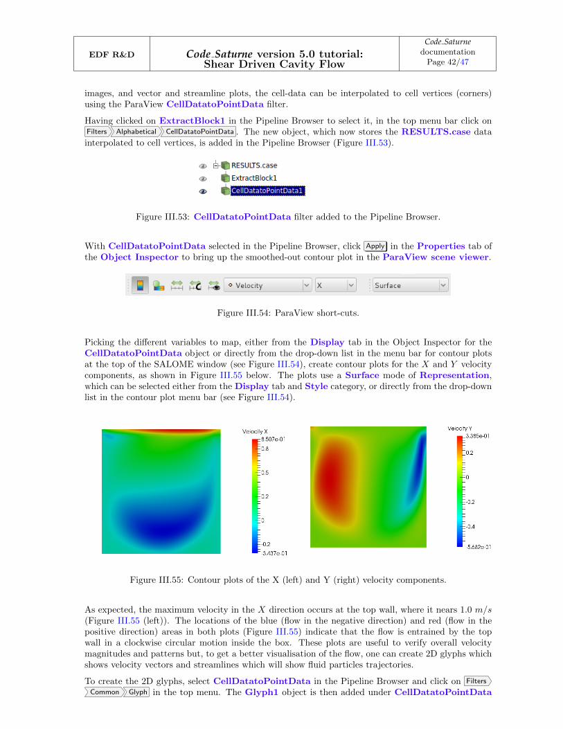
images, and vector and streamline plots, the cell-data can be interpolated to cell vertices (corners)using the ParaView CellDatatoPointData filter.
Having clicked on ExtractBlock1 in the Pipeline Browser to select it, in the top menu bar click onFilters Alphabetical CellDatatoPointData . The new object, which now stores the RESULTS.case datainterpolated to cell vertices, is added in the Pipeline Browser (Figure III.53).
Figure III.53: CellDatatoPointData filter added to the Pipeline Browser.
With CellDatatoPointData selected in the Pipeline Browser, click Apply in the Properties tab ofthe Object Inspector to bring up the smoothed-out contour plot in the ParaView scene viewer.
Figure III.54: ParaView short-cuts.
Picking the different variables to map, either from the Display tab in the Object Inspector for theCellDatatoPointData object or directly from the drop-down list in the menu bar for contour plotsat the top of the SALOME window (see Figure III.54), create contour plots for the X and Y velocitycomponents, as shown in Figure III.55 below. The plots use a Surface mode of Representation,which can be selected either from the Display tab and Style category, or directly from the drop-downlist in the contour plot menu bar (see Figure III.54).
Figure III.55: Contour plots of the X (left) and Y (right) velocity components.
As expected, the maximum velocity in the X direction occurs at the top wall, where it nears 1.0 m/s(Figure III.55 (left)). The locations of the blue (flow in the negative direction) and red (flow in thepositive direction) areas in both plots (Figure III.55) indicate that the flow is entrained by the topwall in a clockwise circular motion inside the box. These plots are useful to verify overall velocitymagnitudes and patterns but, to get a better visualisation of the flow, one can create 2D glyphs whichshows velocity vectors and streamlines which will show fluid particles trajectories.
To create the 2D glyphs, select CellDatatoPointData in the Pipeline Browser and click on Filters
Common Glyph in the top menu. The Glyph1 object is then added under CellDatatoPointData
EDF R&D Code Saturne version 5.0 tutorial:Shear Driven Cavity Flow
Code SaturnedocumentationPage 43/47
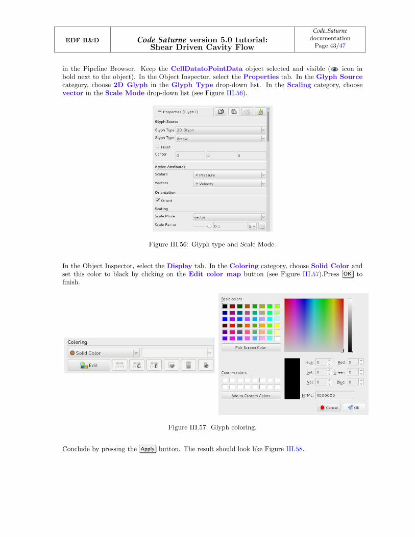
in the Pipeline Browser. Keep the CellDatatoPointData object selected and visible ( icon inbold next to the object). In the Object Inspector, select the Properties tab. In the Glyph Sourcecategory, choose 2D Glyph in the Glyph Type drop-down list. In the Scaling category, choosevector in the Scale Mode drop-down list (see Figure III.56).
Figure III.56: Glyph type and Scale Mode.
In the Object Inspector, select the Display tab. In the Coloring category, choose Solid Color andset this color to black by clicking on the Edit color map button (see Figure III.57).Press OK tofinish.
Figure III.57: Glyph coloring.
Conclude by pressing the Apply button. The result should look like Figure III.58.

EDF R&D Code Saturne version 5.0 tutorial:Shear Driven Cavity Flow
Code SaturnedocumentationPage 44/47
Figure III.58: Contour plot of the velocity with 2D glyphs.
To make it possible to create and locate the streamlines with regard to the Cavity, you are going tocreate a combined image showing the streamlines superimposed on top of the mesh.
First, create the streamlines. With CellDatatoPointData selected in the Pipeline Browser, clickon Filters Common Stream Tracer in the top menu. The SteamTracer object is then added underCellDatatoPointData in the Pipeline Browser. Keep the CellDatatoPointData object selectedand visible ( icon in bold next to the object). In the Object Inspector, select the Display tab. Inthe Coloring category, choose Solid Color in the Color by drop-down list. In the Style category,change the Representation to Wireframe and decrease the Opacity to 0.1 (Figure III.59).
Figure III.59: Selecting the opacity.
The mesh lines displayed in the ParaView scene Viewer should be painted in faint black colour.
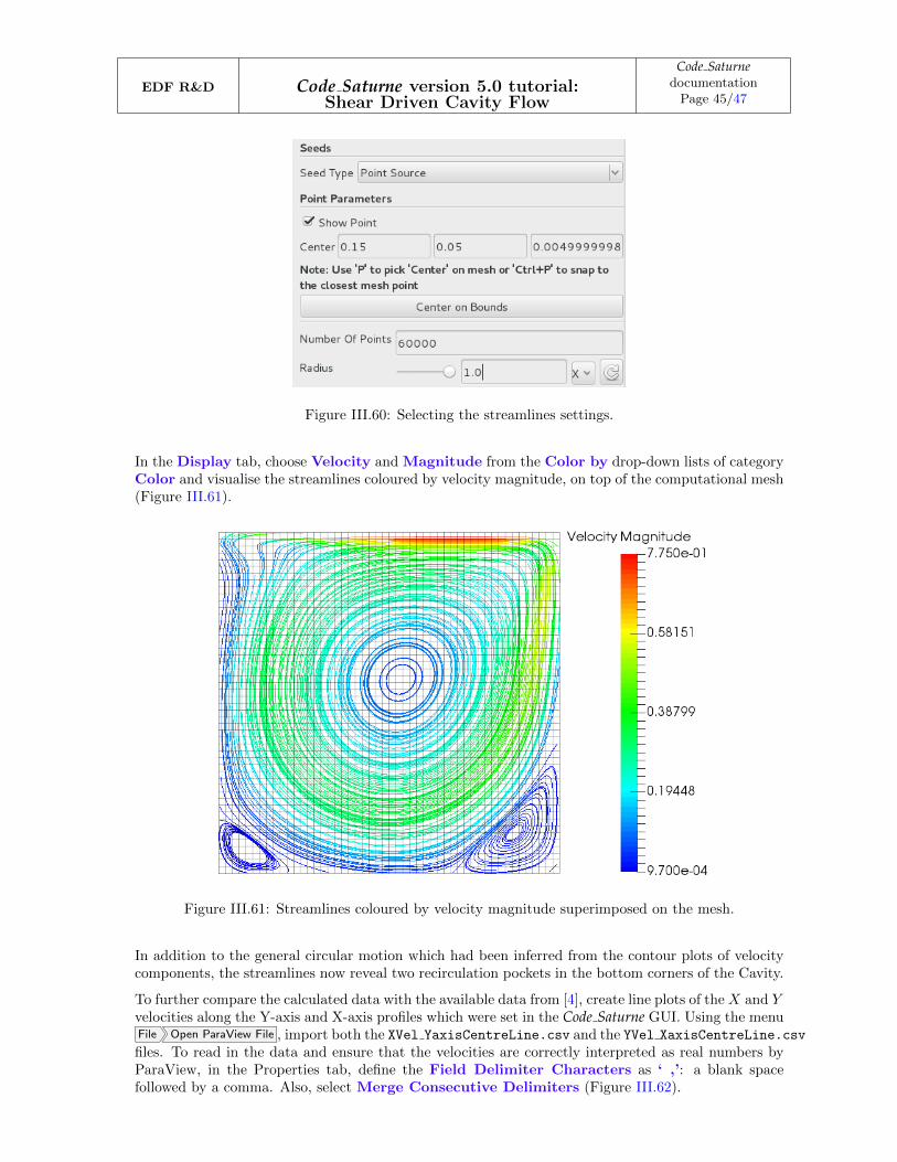
Next, select the StreamTracer1 object in the Pipeline Browser. In the Object Inspector, selectthe Properties tab and modify the default settings for Seeds. Select Point Source for the SeedType, and modify the X and Y coordinates of the seed point to 0.15 and 0.05, respectively. Request60,000 points (Number of Points) and a radius of 1.0 (Radius), as shown in Figure III.60 below.Press Apply to validate your changes.
EDF R&D Code Saturne version 5.0 tutorial:Shear Driven Cavity Flow
Code SaturnedocumentationPage 45/47
Figure III.60: Selecting the streamlines settings.
In the Display tab, choose Velocity and Magnitude from the Color by drop-down lists of categoryColor and visualise the streamlines coloured by velocity magnitude, on top of the computational mesh(Figure III.61).
Figure III.61: Streamlines coloured by velocity magnitude superimposed on the mesh.
In addition to the general circular motion which had been inferred from the contour plots of velocitycomponents, the streamlines now reveal two recirculation pockets in the bottom corners of the Cavity.
To further compare the calculated data with the available data from [4], create line plots of the X and Yvelocities along the Y-axis and X-axis profiles which were set in the Code Saturne GUI. Using the menuFile Open ParaView File , import both the XVel YaxisCentreLine.csv and the YVel XaxisCentreLine.csv
files. To read in the data and ensure that the velocities are correctly interpreted as real numbers byParaView, in the Properties tab, define the Field Delimiter Characters as ‘ ,’: a blank spacefollowed by a comma. Also, select Merge Consecutive Delimiters (Figure III.62).
EDF R&D Code Saturne version 5.0 tutorial:Shear Driven Cavity Flow
Code SaturnedocumentationPage 46/47
Figure III.62: Specifying the velocity profiles.
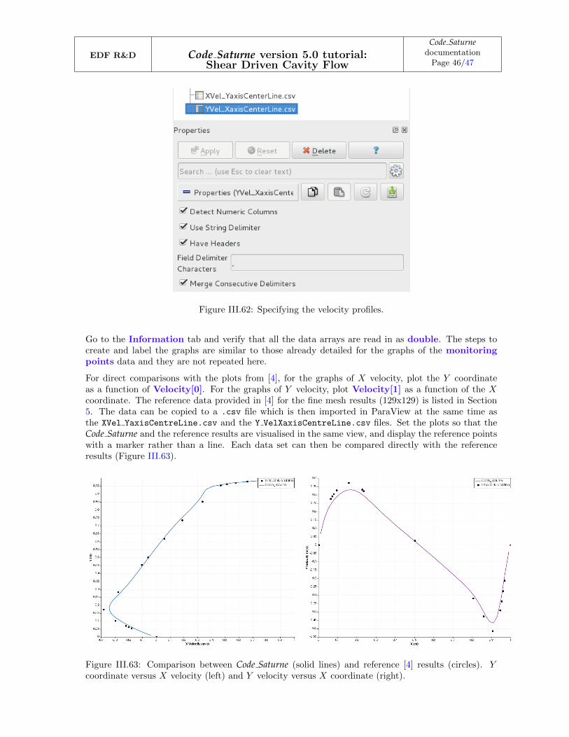
Go to the Information tab and verify that all the data arrays are read in as double. The steps tocreate and label the graphs are similar to those already detailed for the graphs of the monitoringpoints data and they are not repeated here.
For direct comparisons with the plots from [4], for the graphs of X velocity, plot the Y coordinateas a function of Velocity[0]. For the graphs of Y velocity, plot Velocity[1] as a function of the Xcoordinate. The reference data provided in [4] for the fine mesh results (129x129) is listed in Section5. The data can be copied to a .csv file which is then imported in ParaView at the same time asthe XVel YaxisCentreLine.csv and the Y VelXaxisCentreLine.csv files. Set the plots so that theCode Saturne and the reference results are visualised in the same view, and display the reference pointswith a marker rather than a line. Each data set can then be compared directly with the referenceresults (Figure III.63).
Figure III.63: Comparison between Code Saturne (solid lines) and reference [4] results (circles). Ycoordinate versus X velocity (left) and Y velocity versus X coordinate (right).

EDF R&D Code Saturne version 5.0 tutorial:Shear Driven Cavity Flow
Code SaturnedocumentationPage 47/47
Overall, good agreement is obtained with the reference results [4], even though the results withCode Saturne were obtained on a coarser mesh. Running on a finer mesh would make it possibleto capture the velocity extremas with increased accuracy.
4 References[1] www.salome-platform.org
[2] F. Archambeau, N. Mechitoua, M. Sakiz,Code Saturne: a Finite Volume Code for the Computation of Turbulent Incompressible Flows -Industrial Applications,International Journal on Finite Volumes, Vol. 1, 2004.
[3] www.code-saturne.org
[4] U. Ghia, K.N. Ghia, and C.T. Shin,High-Re solutions for incompressible flow using the Navier-Stokes equations and a multigridmethod,Journal of Comp. Phys., Vol. 48, pp. 387-411, 1982.
[5] U. Ayachit,The ParaView Guide: A Parallel Visualization Application,Kitware, 2015, ISBN 978-1930934306
5 Reference Data from [4]To make it easier to replicate the comparative plots of the Code Saturne and reference results, the datafrom [4] (Tables I and II) at Re = 1000 is reproduced in Figure III.3 below. The reference results listedin [4] were obtained on a fine, 129x129 mesh.
Y (m) Ux (m/s) X (m) Uy (m/s)1.00000 1.00000 1.00000 0.000000.97660 0.65928 0.96880 -0.213880.96880 0.57492 0.96090 -0.276690.96090 0.51117 0.95310 -0.337140.95310 0.46604 0.94530 -0.391880.85160 0.33304 0.90630 -0.515500.73440 0.18719 0.85940 -0.426650.61720 0.05702 0.80470 -0.319660.50000 -0.06080 0.50000 0.025260.45310 -0.10648 0.23440 0.322350.28130 -0.27805 0.22660 0.330750.17190 -0.38289 0.15630 0.370950.10160 -0.29730 0.09380 0.326270.07030 -0.22220 0.07810 0.303530.06250 -0.20196 0.07030 0.290120.05470 -0.18109 0.06250 0.274850.00000 0.00000 0.00000 0.00000
Table III.3: X velocity versus Y at the vertical mid-plane and Y velocity versus X at the horizontalmid-plane. Data reproduced from [4]. Re = 1000. 129x129 mesh.