Cobordism and Concordance of Knotsv1ranick/papers/blanloeil2.pdf · knots which naturally arises...
65
Cobordism and Concordance of Knots Vincent Blanlœil March 21, 2007
Transcript of Cobordism and Concordance of Knotsv1ranick/papers/blanloeil2.pdf · knots which naturally arises...
Cobordism and Concordance of Knots
Vincent Blanlœil
March 21, 2007

2
3
to V., V. & A.
!"$#&%'()+*-,-./102!3
Contents
1 Introduction 51.1 History . . . . . . . . . . . . . . . . . . . . . . . . . . . . . . . . 51.2 Definitions . . . . . . . . . . . . . . . . . . . . . . . . . . . . . . . 71.3 Fibered knots . . . . . . . . . . . . . . . . . . . . . . . . . . . . . 141.4 Complex hypersurfaces isolated singularities . . . . . . . . . . . . 141.5 Alexander polynomial . . . . . . . . . . . . . . . . . . . . . . . . 15
2 h-cobordism Theorem and surgeries on manifolds 162.1 Morse functions and handle decompositions of manifolds . . . . . 162.2 h-cobordism Theorem . . . . . . . . . . . . . . . . . . . . . . . . 302.3 Surgery on manifolds . . . . . . . . . . . . . . . . . . . . . . . . . 41
3 Spherical knots 433.1 Alexander polynomial . . . . . . . . . . . . . . . . . . . . . . . . 433.2 S-equivalence . . . . . . . . . . . . . . . . . . . . . . . . . . . . . 433.3 Cobordism of spherical knots . . . . . . . . . . . . . . . . . . . . 46
4 Fibered knots and algebraic knots 494.1 Fibered knots . . . . . . . . . . . . . . . . . . . . . . . . . . . . . 494.2 Algebraic knots . . . . . . . . . . . . . . . . . . . . . . . . . . . . 55
Chapter 1
Introduction
”... the theory of ”Cobordisme” which has,within the few years of its existence,
led to the most penetrating insights intothe topology of differentiable manifolds.”
H. Hopf,International Congress of Mathematics, 1958.
1.1 History
In the early fifties Rohlin [113] and Thom [129] studied the cobordism groups ofmanifolds. At the 1958 International Congress of Mathematicians in Edinburgh,Rene Thom received a Fields Medal for his development of cobordism theory.
Then, Fox and Milnor [37, 38] were the first to study cobordism of knots,i.e., cobordism of embeddings of the circle S1 into the 3-sphere S3. Knot cobor-dism is slightly different from the general cobordism, since its definition is morerestrictive. After Fox and Milnor, Kervaire [65] and Levine [80] studied em-beddings of the n-sphere Sn (or homotopy n-spheres) into the (n + 2)-sphereSn+2, and gave classifications of such embeddings up to cobordism for n ≥ 2.Moreover, Kervaire defined group structures on the set of cobordism classes ofn-spheres embedded in Sn+2, and on the set of concordance classes of embed-dings of Sn into Sn+2. The structures of these groups for n ≥ 2 were clarifiedby Kervaire [65], Levine [80, 81] and Stoltzfus [127].
Note that embeddings of spheres were studied only in the codimension twocase, since in the PL category Zeeman [146] proved that all such embeddings incodimension greater than or equal to three are unknotted, and Stallings [126]proved that it is also true in the topological category (here, one needs to assumethe locally flatness condition), provided that the ambient sphere has dimensiongreater than or equal to five. In the smooth category Haefliger [46] proved thata cobordism of spherical knots in codimension greater than or equal to threeimplies isotopy.
Later people studied embeddings of manifolds, which are not necessaryhomeomorphic to spheres, into codimension two spheres. One motivation comesfrom the topology of complex hupersurfaces near isolated singular points. Moreprecisely, Milnor [100] showed that, in a neighborhood of an isolated singularpoint, a complex hypersurface is homeomorphic to the cone over the algebraicknot associated with the singularity. Hence, the embedded topology of a com-plex hypersurface around an isolated singular point is given by the algebraicknot, which is a special case of a fibered knot. After Milnor’s work, the classof fibered knots has been recognized as an important class of knots to study.Usually algebraic knots are not homeomorphic to spheres, and this motivatedthe study of embeddings of general manifolds (not necessarily homeomorphicto spheres) into spheres in codimension two. Moreover, in the beginning ofthe seventies, Le [76] proved that isotopy and cobordism are equivalent for 1-dimensional algebraic knots. Le proved this for the case of connected (or spher-ical) algebraic 1-knots, and the generalization to arbitrary algebraic 1-knotsfollows easily (for details, see §??).
6 1 Introduction
During Arcata’s symposium of pure mathematics in 1974, Durfee [33] listedseveral unsolved problems about algebraic knots. After Le’s previous result, thefollowing question seems natural
Problem 5([33]): Are cobordant algebraic knots (with K homeomorphic toa sphere) isotopic?
About twenty years later, Du Bois and Michel [30] gave the first examplesof algebraic spherical knots that are cobordant but are not isotopic. Theseexamples motivated the classification of fibered knots up to cobordism.
But we have to wait about twenty years for an answer when Du Bois andMichel [30] gave the first examples of algebraic spherical knots that are cobor-dant but are not isotopic. These examples motivated the classification of fiberedknots up to cobordism.
1.1.1 Contents
This book is organized as follows. In Chapter 1 we give several apropos def-initions to the cobordism theory of knots. The Seifert form associted with aknot is also introduced. In §?? we review the classifications of (simple) spher-ical (2n − 1)-knots with n ≥ 2 up to isotopy and up to cobordism. In §?? wereview the properties of algebraic 1-knots and present the classification theoremof algebraic 1-knots up to cobordism due to Le [76]. In §?? we present theclassifications of simple fibered (2n− 1)-knots with n ≥ 3 up to isotopy and upto cobordism. The classification up to cobordism is based on the notion of thealgebraic cobordism. In order to clarify the definition of algebraic cobordism,we give several explicit examples. We also explain why this relation may notbe an equivalence relation on the set bilinear forms defined on free Z-modulesof finitge rank. The classification of 3-dimensional simple fibered knots up tocobordism is given in §??. In §?? we recall the Fox-Milnor type relation on theAlexander polynomials of cobordant knots. As an application, we show thatthe usual spherical knot cobordism group modulo the subgroup generated bythe cobordism classes of fibered knots is infinitely generated for odd dimensions.In §?? we present several examples of knots with interesting properties in viewof the cobordism theory of knots. In §?? we define the pull back relation forknots which naturally arises from the viewpoint of the codimension two surgerytheory. We illustrate several results on pull back of fibered knot with examples.Some results for even dimensional knots are given in §??, where we explain re-cent results about embedded surfaces in S4 and embedded 4-manifolds in S6.Finally in §??, we give several open problems related to the cobordism theoryof non-spherical knots, where a “non-spherical manifold” refers to a generalmanifold which may not necessarily be a homotopy sphere.
With all the results collected in this paper, we have classifications of knotsup to cobordism in any dimensions. Only the classical case of one dimensionalknots, and the case of three dimensional knots remain not to have completeclassifications.
This book is made of a serie of lectures for graduate students in Louis Pasteuruniversity of Strasbourg during the academic year 2006-2007. The purpose ofthese lectures was to give the opportunity to students to learn topology of highdimensional manifolds while studying knot cobordism.
Many proofs and results in this book are comming from papers writen beforeon the subject, and published in different journals. I want to thank here all my

1.2 Definitions 7
co-authors.
1.1.2 Notations
We will work in the smooth category, but sometimes manifolds might havecorners. When a manifold M has boundary we denote it by ∂M . Moreover, ifM is an oriented manifold with boundary we use the outward first conventionto orient its boundary ∂M . All the homology and cohomology theory used haveinteger coefficients. The symbol ∼= denotes a diffeomorphism between manifoldsor an isomorphism between algebraic objects. An embedding of a manifold Kin a manifold M is denoted by K → M . The closure of X is denoted by X,and its interior is denote by
X or by IntX. We denote by tA the transpose of
a matrix A.
1.2 Definitions
In this section we introduce knot cobordism. We also present some dedtailledconstructions in order to give to the reader a precise idea of the subject.
Since our aim is to study cobordism and concordance of codimension twoembeddings of manifolds which are not necessarily homeomorphic to spheres,we define knots as follows.
Definition 1.1. Let K be a closed n-dimensional manifold embedded in the(n+ 2)-dimensional sphere Sn+2. We suppose that K is
(k − 2)-connected if n = 2k − 1 and k ≥ 2, or
(k − 1)-connected if n = 2k and k ≥ 1.
When K is orientable, we further assume that it is oriented. Then we call K orits (oriented) isotopy class an n-knot, or simply a knot.
An n-knot K is spherical if K is
1. diffeomorphic to the n-dimensional standard sphere Sn for n ≤ 4, or
2. a homotopy n-sphere for n ≥ 5.
Remark 1.2. We use the above definition of a spherical knot for n ≤ 4 in orderto avoid the difficulty related to the smooth Poincare conjecture in dimensionsthree and four.
Remark 1.3. With our definition one dimensional knots may have severalconnected components. But spherical 1-knots are connected and diffeomorphicto S1, see Figure 1.1 and Figure 1.2.
We impose a connectivity condition in Definition 1.1, this is first motivatedby the usual definition of algebraic knot (see Definition ??), and second becauselater we will need connectivity conditions to perform embedded surgeries.
In order to define, and compute, invariants of isotopy and cobordism classesof knots, we will need some algebraic data associated with knots like Seifertforms and Alexander polynomials. In the classical knot theory, i.e., the caseof spherical 1-knots, it is usual to make combinatorial computations associated

8 1 Introduction
Figure 1.1. The trefoil knot is a spherical 1-knot
Figure 1.2. The Hopf link is not a spherical 1-knot
with crossing of planar representations. We will have another approach, ina sense may be more algebraic, since we will do computations using integralbilinear forms.
The first step is to define Seifert manifolds associated with knots.
1.2.1 Seifert manifolds associated with knots
Proposition 1.4. For every oriented n-knot K with n ≥ 1, there exists a com-pact oriented (n+1)-dimensional submanifold V of Sn+2 having K as boundary.Such a manifold V is called a Seifert manifold associated with K. When K isa one dimensional knot, the manifold V is usually called a Seifert surface.
Remark 1.5. Seifert manifolds are not unique. For a given Seifert manifold ofdimension k, one can construct a new one by doing its connected sum with acompact closed k-manifold embedded in Sk+1.
Proof. The construction of Seifert surfaces associated with 1-knots is elemen-tary.
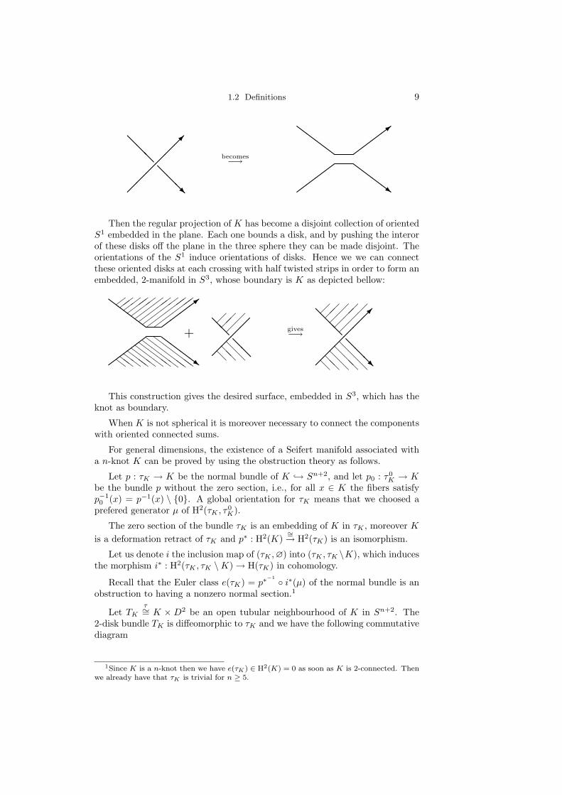
Start by assigning an orientation to each component of the knot, and thenchoose a regular projection into the plane. Around each crossing do the followingmodification:
1.2 Definitions 9
@@
@
@@
@R
becomes−→
ZZ
ZZ
>
Z
ZZ
Z~
Then the regular projection of K has become a disjoint collection of orientedS1 embedded in the plane. Each one bounds a disk, and by pushing the interorof these disks off the plane in the three sphere they can be made disjoint. Theorientations of the S1 induce orientations of disks. Hence we we can connectthese oriented disks at each crossing with half twisted strips in order to form anembedded, 2-manifold in S3, whose boundary is K as depicted bellow:
@@
@
@@
@R
@@@@
@
@@@
@@
@
+@
@
@@
@@@@
@
gives−→
ZZ
ZZ
>
ZZZZ
ZZ
ZZZ
ZZ
ZZ
Z
ZZ
ZZ
ZZ
ZZ
ZZ
ZZZ
ZZ
ZZZ
ZZ
ZZ~
This construction gives the desired surface, embedded in S3, which has theknot as boundary.
When K is not spherical it is moreover necessary to connect the componentswith oriented connected sums.
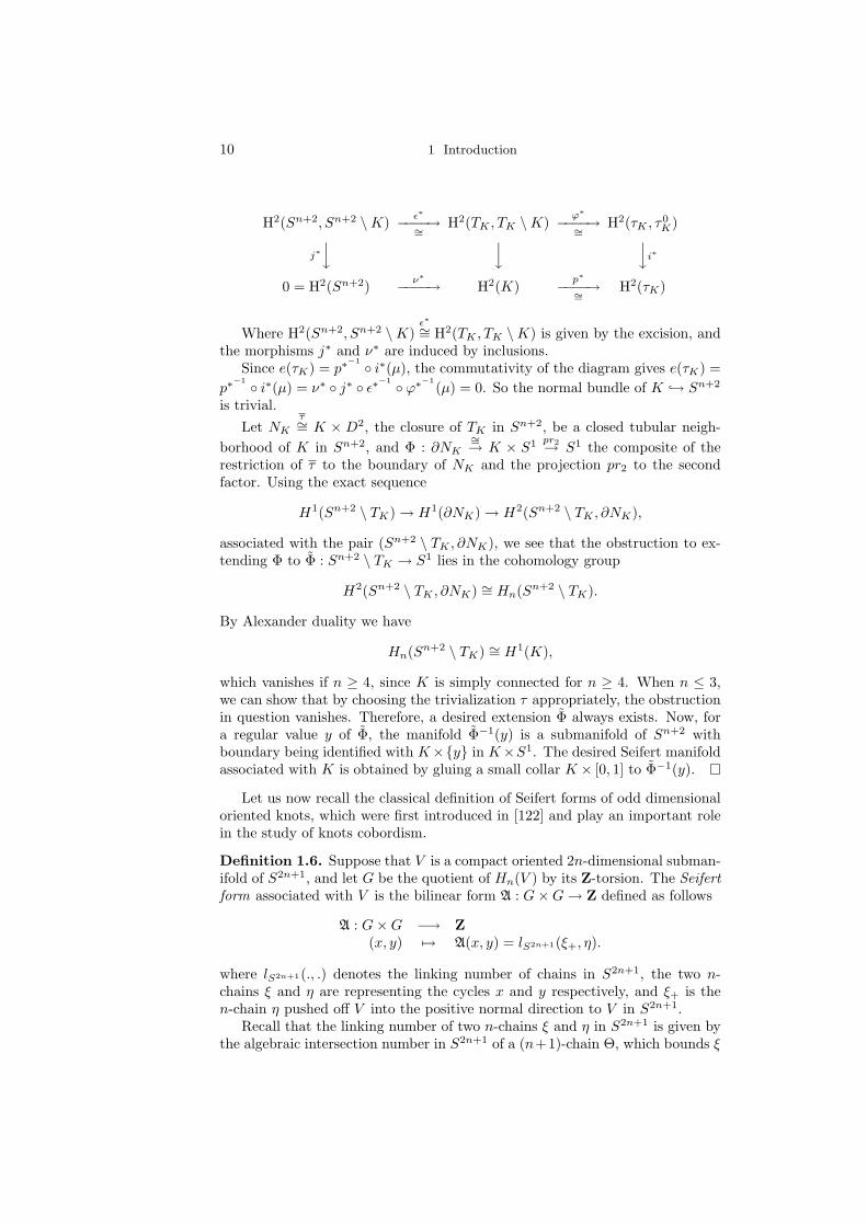
For general dimensions, the existence of a Seifert manifold associated witha n-knot K can be proved by using the obstruction theory as follows.
Let p : τK → K be the normal bundle of K → Sn+2, and let p0 : τ0K → K
be the bundle p without the zero section, i.e., for all x ∈ K the fibers satisfyp−10 (x) = p−1(x) \ 0. A global orientation for τK means that we choosed a
prefered generator µ of H2(τK , τ0K).
The zero section of the bundle τK is an embedding of K in τK , moreover Kis a deformation retract of τK and p∗ : H2(K)
∼=→ H2(τK) is an isomorphism.
Let us denote i the inclusion map of (τK ,∅) into (τK , τK \K), which inducesthe morphism i∗ : H2(τK , τK \K) → H(τK) in cohomology.
Recall that the Euler class e(τK) = p∗−1 i∗(µ) of the normal bundle is an
obstruction to having a nonzero normal section.1
Let TKτ∼= K × D2 be an open tubular neighbourhood of K in Sn+2. The
2-disk bundle TK is diffeomorphic to τK and we have the following commutativediagram
1Since K is a n-knot then we have e(τK) ∈ H2(K) = 0 as soon as K is 2-connected. Thenwe already have that τK is trivial for n ≥ 5.
10 1 Introduction
H2(Sn+2, Sn+2 \K) ε∗−−−−→∼= H2(TK , TK \K)ϕ∗−−−−→∼= H2(τK , τ0
K)
j∗y y yi∗
0 = H2(Sn+2) ν∗−−−−→ H2(K)p∗−−−−→∼= H2(τK)
Where H2(Sn+2, Sn+2 \K)ε∗∼= H2(TK , TK \K) is given by the excision, and
the morphisms j∗ and ν∗ are induced by inclusions.Since e(τK) = p∗
−1 i∗(µ), the commutativity of the diagram gives e(τK) =p∗
−1 i∗(µ) = ν∗ j∗ ε∗−1 ϕ∗−1(µ) = 0. So the normal bundle of K → Sn+2
is trivial.Let NK
τ∼= K × D2, the closure of TK in Sn+2, be a closed tubular neigh-borhood of K in Sn+2, and Φ : ∂NK
∼=→ K × S1 pr2→ S1 the composite of therestriction of τ to the boundary of NK and the projection pr2 to the secondfactor. Using the exact sequence
H1(Sn+2 \ TK) → H1(∂NK) → H2(Sn+2 \ TK , ∂NK),
associated with the pair (Sn+2 \ TK , ∂NK), we see that the obstruction to ex-tending Φ to Φ : Sn+2 \ TK → S1 lies in the cohomology group
H2(Sn+2 \ TK , ∂NK) ∼= Hn(Sn+2 \ TK).
By Alexander duality we have
Hn(Sn+2 \ TK) ∼= H1(K),
which vanishes if n ≥ 4, since K is simply connected for n ≥ 4. When n ≤ 3,we can show that by choosing the trivialization τ appropriately, the obstructionin question vanishes. Therefore, a desired extension Φ always exists. Now, fora regular value y of Φ, the manifold Φ−1(y) is a submanifold of Sn+2 withboundary being identified with K×y in K×S1. The desired Seifert manifoldassociated with K is obtained by gluing a small collar K × [0, 1] to Φ−1(y).
Let us now recall the classical definition of Seifert forms of odd dimensionaloriented knots, which were first introduced in [122] and play an important rolein the study of knots cobordism.
Definition 1.6. Suppose that V is a compact oriented 2n-dimensional subman-ifold of S2n+1, and let G be the quotient of Hn(V ) by its Z-torsion. The Seifertform associated with V is the bilinear form A : G×G→ Z defined as follows
A : G×G −→ Z(x, y) 7→ A(x, y) = lS2n+1(ξ+, η).
where lS2n+1(., .) denotes the linking number of chains in S2n+1, the two n-chains ξ and η are representing the cycles x and y respectively, and ξ+ is then-chain η pushed off V into the positive normal direction to V in S2n+1.
Recall that the linking number of two n-chains ξ and η in S2n+1 is given bythe algebraic intersection number in S2n+1 of a (n+1)-chain Θ, which bounds ξ
1.2 Definitions 11
in S2n+1, and η; or by the algebraic intersection number in D2n+2 of a (n+ 1)-chain Θ, which bounds ξ D2n+2, and a (n + 1)-chain Ω, which bounds η inD2n+2.
By definition a Seifert form associated with an oriented (2n − 1)-knot Kis the Seifert form associated with V , where V is a Seifert manifold associatedwith K. A matrix representative of a Seifert form with respect to a basis of Gis called a Seifert matrix.
Remark 1.7. One can as well define the Seifert form A′(x, y) to be the linkingnumber of ξ and η+ instead of ξ+ and η, where ξ+ is the n-cycle ξ pushed off Vinto the positive normal direction to V in S2n+1. There is no essential differencebetween the two forms A and A′. However some formulas may take differentforms.
More precisely, for a given n-chain ξ in F we denote by ξ− the n-chain ξpushed off V into the negative normal direction to V in S2n+1. Then we have
lS2n+1(ξ, η+) = lS2n+1(ξ−, η),
and recalllS2n+1(ξ, η) = (−1)n+1lS2n+1(η, ξ).
According to these formulas we get
A(x, y) = lS2n+1(ξ+, η)A(x, y) = (−1)n+1lS2n+1(η, ξ+)A(x, y) = (−1)n+1A′(y, x)
So if A a the Seifert matrix associated with A and A′ is the Seifert matrixassociated with A′ we have A′ = (−1)n+1AT
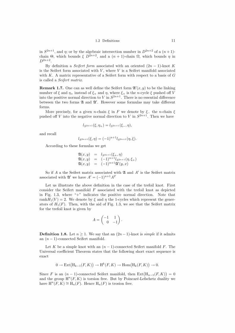
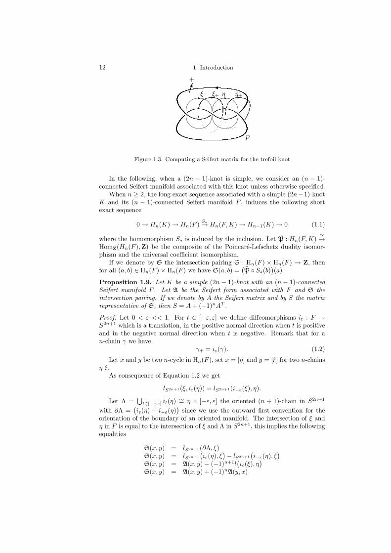
Let us illustrate the above definition in the case of the trefoil knot. Firstconsider the Seifert manifold F associated with the trefoil knot as depictedin Fig. 1.3, where “+” indicates the positive normal direction. Note thatrankH1(V ) = 2. We denote by ξ and η the 1-cycles which represent the gener-ators of H1(F ). Then, with the aid of Fig. 1.3, we see that the Seifert matrixfor the trefoil knot is given by
A =(−1 1
0 −1
).
Definition 1.8. Let n ≥ 1. We say that an (2n− 1)-knot is simple if it admitsan (n− 1)-connected Seifert manifold.
Let K be a simple knot with an (n− 1)-connected Seifert manifold F . TheUniversal coefficient Theorem states that the following short exact sequence isexact
0 → Ext(Hk−1(F,K)
)→ Hk(F,K) → Hom
(Hk(F,K)
)→ 0.
Since F is an (n − 1)-connected Seifert manifold, then Ext(Hn−1(F,K)
)= 0
and the group Hn(F,K) is torsion free. But by Poincare-Lefschetz duality wehave Hn(F,K) ∼= Hn(F ). Hence Hn(F ) is trosion free.
12 1 Introduction
+
# "!
# "!
ξ- ξ+- η- η+-
F
Figure 1.3. Computing a Seifert matrix for the trefoil knot
In the following, when a (2n − 1)-knot is simple, we consider an (n − 1)-connected Seifert manifold associated with this knot unless otherwise specified.
When n ≥ 2, the long exact sequence associated with a simple (2n−1)-knotK and its (n − 1)-connected Seifert manifold F , induces the following shortexact sequence
0 → Hn(K) → Hn(F ) S∗→ Hn(F,K) → Hn−1(K) → 0 (1.1)
where the homomorphism S∗ is induced by the inclusion. Let P : Hn(F,K)∼=→
HomZ(Hn(F ),Z) be the composite of the Poincare-Lefschetz duality isomor-phism and the universal coefficient isomorphism.
If we denote by S the intersection pairing S : Hn(F ) × Hn(F ) → Z, thenfor all (a, b) ∈ Hn(F )×Hn(F ) we have S(a, b) =
(P S∗(b)
)(a).
Proposition 1.9. Let K be a simple (2n − 1)-knot with an (n − 1)-connectedSeifert manifold F . Let A be the Seifert form associated with F and S theintersection pairing. If we denote by A the Seifert matrix and by S the matrixrepresentative of S, then S = A+ (−1)nAT .
Proof. Let 0 < ε << 1. For t ∈ [−ε, ε] we define diffeomorphisms it : F →S2n+1 which is a translation, in the positive normal direction when t is positiveand in the negative normal direction when t is negative. Remark that for an-chain γ we have
γ+ = iε(γ). (1.2)
Let x and y be two n-cycle in Hn(F ), set x = [η] and y = [ξ] for two n-chainsη ξ.
As consequence of Equation 1.2 we get
lS2n+1(ξ, iε(η)) = lS2n+1(i−ε(ξ), η).
Let Λ =⋃t∈[−ε,ε] it(η) ∼= η × [−ε, ε] the oriented (n + 1)-chain in S2n+1
with ∂Λ =(iε(η) − i−ε(η)
)since we use the outward first convention for the
orientation of the boundary of an oriented manifold. The intersection of ξ andη in F is equal to the intersection of ξ and Λ in S2n+1, this implies the followingequalities
S(x, y) = lS2n+1(∂Λ, ξ)S(x, y) = lS2n+1
(iε(η), ξ
)− lS2n+1
(i−ε(η), ξ
)S(x, y) = A(x, y)− (−1)n+1l
(iε(ξ), η
)S(x, y) = A(x, y) + (−1)nA(y, x)
1.2 Definitions 13
rrK0
Sn+2 × 0
rrK1
Sn+2 × 1
Sn+2 × [0, 1]
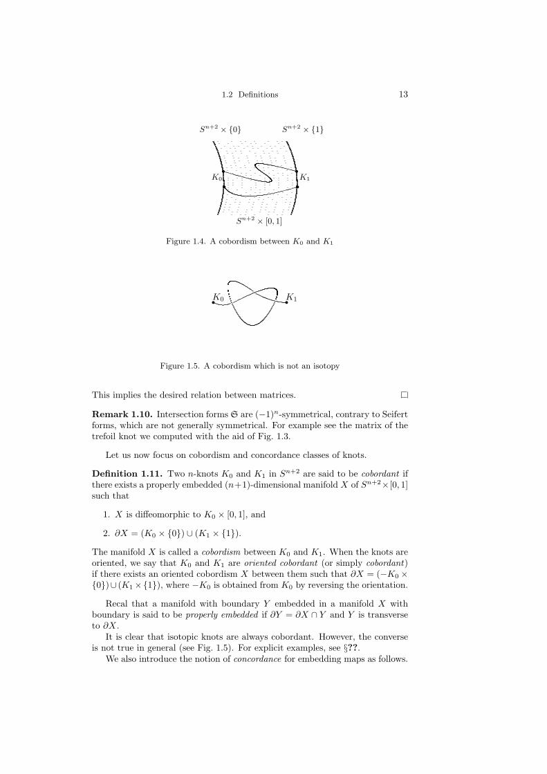
Figure 1.4. A cobordism between K0 and K1
rK0 rK1
Figure 1.5. A cobordism which is not an isotopy
This implies the desired relation between matrices.
Remark 1.10. Intersection forms S are (−1)n-symmetrical, contrary to Seifertforms, which are not generally symmetrical. For example see the matrix of thetrefoil knot we computed with the aid of Fig. 1.3.
Let us now focus on cobordism and concordance classes of knots.
Definition 1.11. Two n-knots K0 and K1 in Sn+2 are said to be cobordant ifthere exists a properly embedded (n+1)-dimensional manifold X of Sn+2×[0, 1]such that
1. X is diffeomorphic to K0 × [0, 1], and
2. ∂X = (K0 × 0) ∪ (K1 × 1).
The manifold X is called a cobordism between K0 and K1. When the knots areoriented, we say that K0 and K1 are oriented cobordant (or simply cobordant)if there exists an oriented cobordism X between them such that ∂X = (−K0 ×0)∪ (K1×1), where −K0 is obtained from K0 by reversing the orientation.
Recal that a manifold with boundary Y embedded in a manifold X withboundary is said to be properly embedded if ∂Y = ∂X ∩ Y and Y is transverseto ∂X.
It is clear that isotopic knots are always cobordant. However, the converseis not true in general (see Fig. 1.5). For explicit examples, see §??.
We also introduce the notion of concordance for embedding maps as follows.

14 1 Introduction
Definition 1.12. Let K be a closed n-dimensional manifold. We say that twoembeddings fi : K → Sn+2, i = 0, 1, are concordant if there exists a properembedding Φ : K × [0, 1] → Sn+2 × [0, 1] such that Φ|K×i = fi : K × i →Sn+2 × i, i = 0, 1.
Where an embedding map ϕ : Y → X between manifolds with boundary issaid to be proper if ∂Y = ϕ−1(∂X) and Y is transverse to ∂X.
Remark 1.13. Concordant knots are cobordant, but the converse is not true ingeneral. See Theorem ?? for the spherical case and Remark ?? for non sphericalexamples.
Cobordant knots are diffeomorphic. Hence, to have a cobordism between twogiven knots, we need to have topological informations about the knots. Since asimple fibered (2n − 1)-knot is the boundary of the closure of a fiber, which isan (n− 1)-connected Seifert manifold associated with the knot, by consideringthe above exact sequence (1.1) we can use the kernel and the cokernel of thehomomorphism S∗ to get topological data of the knot. Note that in the caseof spherical knots, these considerations are not necessary since S∗ and S∗ areisomorphisms.
1.3 Fibered knots
Definition 1.14. We say that an oriented n-knot K is fibered if there exists asmooth fibration φ : Sn+2 \K → S1 and a trivialization τ : NK → K ×D2 of aclosed tubular neighborhood NK of K in Sn+2 such that φ|NK\K coincides withπ τ |NK\K , where π : K × (D2 \ 0) → S1 is the composition of the projectionto the second factor and the obvious projection D2 \ 0 → S1. Note that thenthe closure of each fiber of φ in Sn+2 is a compact (n+ 1)-dimensional orientedmanifold whose boundary coincides with K. We shall often call the closure ofeach fiber simply a fiber.
Furthermore, for n ≥ 1 we say that a fibered (2n − 1)-knot K is simple ifeach fiber of φ is (n− 1)-connected.
Though the notion of fibered knot it is much more restrictive, this definitionwill give additional data, like monodromy and variation map see Chapter 4,which are very usefull.
When K is a fibered knot, the closure of a fiber is always a Seifert manifoldassociated with K.
In the following, for a fibered (2n−1)-knot, we use the Seifert form associatedwith a fiber unless otherwise specified.
Moreover the definition of fibered knots gives a topological framework foralgebraic knots associated with isolated singularities.
1.4 Complex hypersurfaces isolated singularities
One motivation for Definition 1.1 is the study of the topology of isolated singu-larities of complex hypersurfaces.
Let f : Cn+1, 0 → C, 0 be a holomorphic function germ with an isolatedsingularity at the origin. If ε > 0 is sufficiently small, then Kf = f−1(0)∩S2n+1
ε
1.5 Alexander polynomial 15
is a (2n − 1)-dimensional manifold which is naturally oriented, where S2n+1ε is
the sphere in Cn+1 of radius ε centered at the origin. Furthermore, its (oriented)isotopy class in S2n+1
ε = S2n+1 does not depend on the choice of ε (see [100]).
Definition 1.15. We call Kf the algebraic knot associated with f .
Since the pair (D2n+2ε , f−1(0)∩D2n+2
ε ) is homeomorphic to the cone over thepair (S2n+1
ε ,Kf ), the algebraic knot completely determines the local embeddedtopological type of f−1(0) near the origin, where D2n+2
ε is the disk in Cn+1 ofradius ε centered at the origin.
Milnor [100] considers only polynomial functions. However, it is knownthat a holomorphic function germ with an isolated critical point is topologicallyequivalent to a polynomial function germ.
In [100], Milnor proved that, when n ≥ 2, algebraic knots associated withisolated singularities of holomorphic function germs f : Cn+1, 0 → C, 0 are(2n−1)-dimensional closed, oriented and (n−2)-connected submanifolds of thesphere S2n+1. This means that algebraic knots are some knots in the senseof Definition 1.1. Moreover, the complement of an algebraic knot Kf in thesphere S2n+1 admits a fibration over the circle S1, and the closure of each fiberis a compact 2n-dimensional oriented (n − 1)-connected submanifold of S2n+1
which has Kf as boundary. Note that an algebraic knot is always a simplefibered knot.
1.5 Alexander polynomial
The Alexander polynomial associated with a knot K was initially defined forspherical 1-knots, and was computed with a combinatorial presentation of 1-knots, i.e., crossings. But, with the aid of a Seifert form associated with a knotit is possible to define Alexander polynomials for knots of every dimension.
Let K a (2n− 1)-knot, with n ≥ 1. Set A be a Seifert form for K associatedwith a Seifert manifold F . The polynomial
∆A(t) = det(tA+ (−1)n tA)
of Z[t, t−1], is well defined up to units of Z[t, t−1], and is called the Alexanderpolynomial of K.
Remark that the Alexander polynomial is defined up to units of Z[t, t−1]since the Seifert manifold associated with the knot is not unique.
Chapter 2
h-cobordism Theorem and surgeries on
manifolds
Macbeth ...— What is the night?Lady Macbeth Almost at odds
with morning, which is which.Macbeth Act III, sc IV
The goal of this Chapter is to prove the h-cobordism Theorem. In fact wewill prove a slightly more general theorem, which is called s-cobordism Theorem.We choose to give the proof of the s-cobordism theorem because of the similarityof the proofs, though we need to consider Whitehead torsions to prove the s-cobordism Theorem. The first step is to introduce Morse theory and handlebodydecomposition for manifolds. In conclusion of this Chapter we will describemodifications of manifolds called surgeries.
2.1 Morse functions and handle decompositions ofmanifolds
In this section we recall briefly some classical results on Morse theory, we referto [97] and [89] for detailed proofs.
We will consider functions defined on manifolds. LetMn be a n-dimensionnalmanifold with n ∈ N∗, recall that we only consider smooth manifolds. A func-tion f : M → R is smooth if there exists a local coordinate system (x1, . . . , xn)around each point p of M in which f is C∞. By opposition we define
Definition 2.1. A point p0 ∈M is a critical point of the function f : M → R
if∂f
∂xi(p0) = 0, i = 1, . . . , n.
It is easy to check that this definition does not depend on the choice of acoordinate system.
Definition 2.2. We say that a critical point p0 of f is non-degenerate if thedeterminant
Hf (p0) = det
∂2f∂x2
1(p0) . . . ∂2f
∂x1∂xn(p0)
......
∂2f∂xn∂x1
(p0) . . . ∂2f∂x2
n(p0)
is not zero, and it is degenerate if Hf (p0) = 0. We call Hf (p0) the Hessian of fat the critical point p0.
2.1 Morse functions and handle decompositions of manifolds 17
Let (x1, . . . , xn) and (y1, . . . , yn) be two coordinate systems, and set
J(p0) =
∂x1∂y1
(p0) . . . ∂x1∂yn
(p0)...
...∂xn
∂y1(p0) . . . ∂xn
∂yn(p0)
,
which is usually called the Jacobian matrix of the coordinate transformationevaluated at p0.
If we denote by Hxf (p0) the Hessian of f in the coordinate system x =
(x1, . . . , xn), then by direct computation we get
Hyf (p0) = tJ(p0)Hx
f (p0)J(p0).
Definition 2.3. A real number c is called a critical value of a f : M → R ifthere exists a critical point p0 ∈M such that f(p0) = c.
Since the Jacobian of the coordinate transformation at a point p0 has anon-zero determinant, then we have
detHyf (p0) = det
(tJ(p0)
)det
(Hxf (p0)
)det
(J(p0)
).
But the determinant of the Jacobian of any coordinate transformation at apoint p0 has a non-zero determinant. Hence detHy
f (p0) 6= 0 if and only ifdetHx
f (p0) 6= 0, and the property of a critical point of a function being non-degenerate or degenerate does not depend on the choice of a coordinate systemat p0.
Definition 2.4. A function f : M → R is called a Morse function if everycritical point of f is non-degenerate.
Theorem 2.5 (Morse Lemma). Let p0 be a non-degenerate critical point off : M → R. Then there exists a local coordinate system (x1, . . . , xn) at p0 suchthat with respect to these cooordinates f has the form
−x21 − . . .− x2
λ + x2λ+1 + . . .+ x2
n + f(p0)
Sylvester’s law implies that 0 ≤ λ ≤ n is well defined and do not dependon the choice of the coordinate system. Since λ depends only on the function fand the critical point p0, then we define
Definition 2.6. The integer λ is called the index of the non-degenerate criticalpoint p0 of the function f .
Proof of Morse Lemma. Without loss of generality one can assume that f(p0) =0, and let (x1, . . . , xn) be a local coordinate system around the origin p0. Sincef(p0) = 0, then according to the fundamental Theorem of calculus one can find
n smooth functions hi(x) =∫ 1
0
∂f
∂xi(tx)dt, i = 1, . . . , n such that
f(x1, . . . , xn) =n∑i=1
xi hi(x1, . . . , xn).
18 2 h-cobordism Theorem and surgeries on manifolds
With this decomposition we get∂f
∂xi(0, . . . , 0) = hi(0, . . . , 0) for i = 1, . . . , n.
Now, since the origin p0 in the local coordinate system (x1, . . . , xn) is acritical point for the function f , then we have hi(0, . . . , 0) = 0 for i = 1, . . . , n.As made before for f , for each hi, i = 1, . . . , n one can find n smooth functionshi,j , j = 1, . . . , n such that
hi(x1, . . . , xn) =n∑j=1
xj hi,j(x1, . . . , xn).
Putting these decompositions all together, we get
f(x1, . . . , xn) =n∑
i,j=1
xixj hi,j(x1, . . . , xn),
setting Hi,j = hi,j+hj,i
2 gives Hi,j = Hj,i and the following quadratic represen-tation of f
f(x1, . . . , xn) =n∑
i,j=1
xixj Hi,j(x1, . . . , xn). (2.1)
We will now reduce this representation to the wanted one using the Gaussalgorithm on quadratic forms.
The computation of the second order partial derivative of 2.1 gives
∂2f
∂xi∂xj(0, . . . , 0) = 2Hi,j(0, . . . , 0).
Since p0 is a non-degenerate critical point of the function f , then we havedetHf (p0) = detHx
f (0, . . . , 0) = det(Hi,j(0, . . . , 0)
)i,j6= 0. Moreover, up to a
change of local coordinates, we can assume that
∂2f
∂x21
(0, . . . , 0) 6= 0,
hence since the functions Hi,j are continuous this gives H1,1 6= 0 (eventually ona smaller neighborhood of p0 than the one of the local coordinate system).
Now for an appropriate choice of local coordinate (X1, x2, . . . , xn) the func-tion f is of the form
f(X1, x2, . . . , xn) = ±X21 + ϕ(x2, . . . , xn) (2.2)
with ϕ(x2, . . . , xn) a quadratic form with n−1 variables x2, . . . , xn. By inductionon the number of variables one can reduce the function f to the desired form.
Corollary 2.7. Let f : M → R be a Morse function. Any non-degeneratecritical point of f is isolated, and when M is a compact n-manifold f admitsfinitely many critical points.
Proof. According to Morse Lemma, in a small coordinate neighbourhood of acritical point p0, the function f is of the form −x2
1 − . . . − x2λ + x2
λ+1 + . . . +x2n + f(p0). So the origin, i.e., the point p0, is the only critical point in the
2.1 Morse functions and handle decompositions of manifolds 19
coordinate neighbourhood of p0. Recall that for a Morse function any criticalpoint is non-degenerate.
Assume that the Morse function f admits infinitely many distinct criticalpoints (pi)i∈I where I is an infinite set. Since non-degenerated critical pointsare isolated there exists disjoint open sets (Ui)i∈I such that Ui ⊂ M containsonly one critical point pi. First construct U ⊂ M an open set such that for alli in I the point pi is not in U , then the infinite cover
M ⊂ U⋃i∈I
Ui
can’t be reduced to a finite one. This is in contradiction with the hypothesis ofcompactness for M .
Finally the Morse function f admits only finitely many critical points.
Now we will see that every function f : M → R on a compact manifold canbe approximate by a Morse function.
Definition 2.8. Let M be a compact manifold, and let ε > 0 be a real. Afunction f : M → R is a C2
ε -approximation of a function ϕ : M → R if thereexists a compact covering M ⊂
⋃i=1,...,m Yi and on each compact Yi ⊂ M ,
i = 1, . . . ,m the following hold
1. ∀y ∈ Yi |f(y)− g(y)| < ε,
2. ∀y ∈ Yi |∂f(y)∂xj− ∂g(y)
∂xj| < ε, j = 1, . . . , n,
3. ∀y ∈ Yi | ∂2f(y)
∂xj∂xk− ∂2g(y)
∂xj∂xk| < ε, j, k = 1, . . . , n.
Theorem 2.9 (Existence of Morse functions). Let M be a compact manifoldwithout boundary, and f : M → R a smooth function. Then for each realε > 0 there exists a Morse function ψ on M which is a C2
ε -approximation off . Moreover one can assume that the critical values associated with distinctscritical points of ψ are distincts.
We refer to [89] for a detailed proof of this Theorem.
Using Morse functions defined on a manifold M , we will explain now how toconstruct some particular tangent vector fields on M . These vector fields makeeasier to understand the behaviour of the manifold around the critical points ofthe Morse functions.
Before, recall, that for a given vector v ∈ TpM the directional derivative of afunction f : M → R can be defined as follows. Let c(τ) =
(x1(τ), . . . , xn(τ)
)be
a curve in M such that c(0) = p anddcdt
(0) = v. Then the directional derivativeof f in the direction v at p is the real function defined on M
v.f =n∑i=1
dxidt
(0)∂f
∂xi.
When X is a tangent vector field on M , i.e., to each point p in M we associatea tangent vector X(p) in Tp(M), we extend this definition. We compute the

20 2 h-cobordism Theorem and surgeries on manifolds
0 x1, . . . , xλ
xλ+1, . . . , xn
- --
?
?
?
6
6
6
: *
1
3
XzHj
AU
BBN
Pq
JJ
CCW
Qs
JJ
AU
9
)
+
XyHYAK
BBM
PiJJ]
CCO
QkJJ]
AK
Figure 2.1. The gradient vector field of x21 − . . .− x2
λ + x2λ+1 + . . . + x2
n
directional derivative of f in the direction X(p) at p. Then we can differentiatef with respect to X as well. A tangent vector field is defined by
X(p) =n∑i=1
ξi(p)( ∂
∂xi
)p,
where ξi(p) are smooth functions defined on a coordinate system at p for i =1, . . . , n. Then set
(X.f
)(p) =
( n∑i=1
ξi(p)( ∂
∂xi
)p.f
)(p)
Now let us consider the gradient vector field of a Morse function f : M → Rin a small neighborhood of a critical point for f . We saw that in an appropriatelocal coordinate system (x1, . . . , xn) the function f has the form
−x21 − . . .− x2
λ + x2λ+1 + . . .+ x2
n.
Its gradient vector field is
∇f = −2x1∂
∂x1− . . .− 2xλ
∂
∂xλ+ 2xλ+1
∂
∂xλ+1+ . . .+ 2xn
∂
∂xn
Remark that ∇f .f =n∑i=1
(∂f
∂xi)2 ≥ 0, and
(∇f .f
)(p) > 0 when p is not a
critical point of the Morse function f . This inequality means that locally thegradient vector field of f follows a direction into which f is increasing.
This induces the following definition.
Definition 2.10. We say that a vector field X on M is a gradient like vectorfield for the Morse function f : M → R if
1.(X.f
)(p) > 0 for any non-critical point p ∈M ,
2. around any critical point of f there exists an appropriate coordinate sys-tem such that X = ∇f .
Theorem 2.11. Let f : M → R be a Morse function on a compact manifold.Then there exists a gradient like vector field on M .
2.1 Morse functions and handle decompositions of manifolds 21
A way to prove this Theorem is to glue all together gradient vector fields off defined on a finite number of coordinate neighbourhoods. We refer to [89] fora detailed proof.
We illustrate the utility of gradient like vector fields with the two followingPropositions.
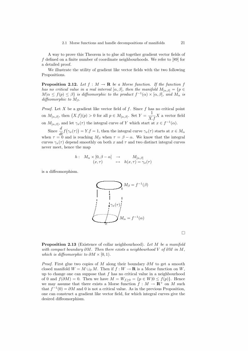
Proposition 2.12. Let f : M → R be a Morse function. If the function fhas no critical value in a real interval [α, β], then the manifold M[α,β] = p ∈M |α ≤ f(p) ≤ β is diffeomorphic to the product f−1(α) × [α, β], and Mα isdiffeomorphic to Mβ.
Proof. Let X be a gradient like vector field of f . Since f has no critical point
on M[α,β], then(X.f
)(p) > 0 for all p ∈ M[α,β]. Set Y =
1X.f
X a vector field
on M[α,β], and let γx(τ) the integral curve of Y which start at x ∈ f−1(α).
Sinced
dtf(γx(τ)
)= Y.f = 1, then the integral curve γx(τ) starts at x ∈Mα
when τ = 0 and is reaching Mβ when τ = β − α. We know that the integralcurves γx(τ) depend smoothly on both x and τ and two distinct integral curvesnever meet, hence the map
h : Mα × [0, β − α] → M[α,β]
(x, τ) 7→ h(x, τ) = γx(τ)
is a diffeomorphism.
γx(τ)rrx
Mα = f−1(α)
Mβ = f−1(β)
6
Proposition 2.13 (Existence of collar neighbourhood). Let M be a manifoldwith compact boundary ∂M . Then there exists a neighbourhood V of ∂M in M ,which is diffeomorphic to ∂M × [0, 1).
Proof. First glue two copies of M along their boundary ∂M to get a smoothclosed manifold W = M ∪∂ M . Then if f : W → R is a Morse function on W ,up to change one can suppose that f has no critical value in a neighbourhoodof 0 and f(∂M) = 0. Then we have M = Wf≥0 = p ∈ W |0 ≤ f(p). Hencewe may assume that there exists a Morse function f : M → R+ on M suchthat f−1(0) = ∂M and 0 is not a critical value. As in the previous Proposition,one can construct a gradient like vector field, for which integral curves give thedesired diffeomorphism.
22 2 h-cobordism Theorem and surgeries on manifolds
∂M
M
V =
2.1.1 Handle decompositions of manifolds
In this subsection we will use Morse functions to describe handle decompositionsof compact manifolds.
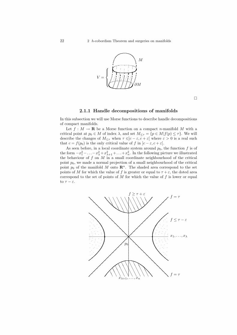
Let f : M → R be a Morse function on a compact n-manifold M with acritical point at p0 ∈M of index λ, and set M≤τ = p ∈M |f(p) ≤ τ. We willdescribe the changes of M≤τ when τ ∈]c − ε, c + ε[ where ε > 0 is a real suchthat c = f(p0) is the only critical value of f in ]c− ε, c+ ε[.
As seen before, in a local coordinate system around p0, the function f is ofthe form −x2
1− . . .−x2λ+x2
λ+1 + . . .+x2n. In the following picture we illustrated
the behaviour of f on M in a small coordinate neighbourhood of the criticalpoint p0, we made a normal projection of a small neighbourhood of the criticalpoint p0 of the manifold M onto Rn. The shaded area correspond to the setpoints of M for which the value of f is greater or equal to τ + ε, the doted areacorrespond to the set of points of M for which the value of f is lower or equalto τ − ε.
AAA
AAAA
AAAA
AAAA
AAAA
AAAA
AAAA
AAA
AAAAA
AA
AAA
AA
A
AA
AA
AA
AA
AA
AA
AA
AA
AA
AA
AA
AA
AAA
f = τ
f = τ
f ≤ τ − ε
x1, . . . , xλ
f ≥ τ + ε
xλ+1, . . . , xn
p0

2.1 Morse functions and handle decompositions of manifolds 23
Definition 2.14. The product manifold Dλ ×Dn−λ is called a λ-handle, andthe λ-disk Dλ × 0 ⊂ Dλ ×Dn−λ is called the core of the handle.
In the following picture we glued a λ-handle Dλ×Dn−λ, along Dλ−1×Dn−λ,to the boundary of the set of points of M for which f takes value lower or equalto τ − ε.
AAA
AAAA
AAAA
AAAA
AAAA
AAAA
AAAA
AAA
AAAAA
AA
AAA
AA
A
AA
AA
AA
AA
AA
AA
AA
AA
AA
AA
AA
AA
AAA
Dλ ×Dn−λ
@@R
AAU
BBBN
CCW
@@I
AAK
BBBM
CCO
With the gradient like vector field depicted by the arrows on the picture, onecan see that, after smoothing, the manifold M≤τ−ε∪Dλ×Dn−λ is diffeomorphicto M≤τ+ε.
Remark 2.15. Let c1, . . . , ck the distinct critical values of a Morse functionf : M → R defined on a compact manifold M without boundary. Let ε > 0 areal small enough, then the following hold
1. M≤c1−ε = ∅,
2. M≤c1+ε = Dn, is a 0-handle,
3. M≤ck+ε = M .
LetX be a n-manifold with non-empty boundary, and let ϕ : Sλ−1×Dn−λ →∂M be an embedding. Using ϕ we can attach a λ-handle to X. Set Y =X ∪ϕ (Dλ × Dn−λ), which is the manifold obtained from X by gluing the λ-handle Dλ ×Dn−λ to ∂X along ϕ(Sλ−1 ×Dn−λ). After smoothing corners ifnecessary we can assume that Y is smooth.
Definition 2.16. We say that Y is obtained by attaching a λ-handle to X,and ϕ is called the attaching map of the λ-handle. We will use the notationY = X ∪ (ϕλ). The disk Dλ × 0 is called the core of the λ-handle, and thesphere 0 × Sn−λ−1 is called the transverse sphere of the λ-handle.
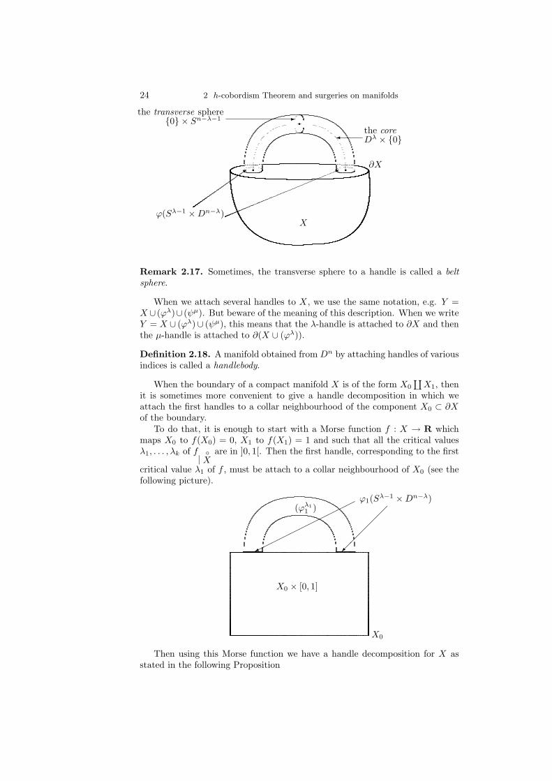
24 2 h-cobordism Theorem and surgeries on manifolds
q qq
X
∂X
ϕ(Sλ−1 ×Dn−λ)
* :
the coreDλ × 0
the transverse sphere0 × Sn−λ−1 -
Remark 2.17. Sometimes, the transverse sphere to a handle is called a beltsphere.
When we attach several handles to X, we use the same notation, e.g. Y =X ∪ (ϕλ)∪ (ψµ). But beware of the meaning of this description. When we writeY = X ∪ (ϕλ)∪ (ψµ), this means that the λ-handle is attached to ∂X and thenthe µ-handle is attached to ∂(X ∪ (ϕλ)).
Definition 2.18. A manifold obtained from Dn by attaching handles of variousindices is called a handlebody.
When the boundary of a compact manifold X is of the form X0
∐X1, then
it is sometimes more convenient to give a handle decomposition in which weattach the first handles to a collar neighbourhood of the component X0 ⊂ ∂Xof the boundary.
To do that, it is enough to start with a Morse function f : X → R whichmaps X0 to f(X0) = 0, X1 to f(X1) = 1 and such that all the critical valuesλ1, . . . , λk of f
|X
are in ]0, 1[. Then the first handle, corresponding to the first
critical value λ1 of f , must be attach to a collar neighbourhood of X0 (see thefollowing picture).
ϕ1(Sλ−1 ×Dn−λ)
X0
X0 × [0, 1]
(ϕλ11 )
Then using this Morse function we have a handle decomposition for X asstated in the following Proposition

2.1 Morse functions and handle decompositions of manifolds 25
Proposition 2.19 (Handle decomposition of boundary manifolds). Let X be acompact manifold with boundary ∂X = X0
∐X1. Then X possesses a handle-
body decomposition up to diffeomorphism
X = X0 × [0, 1]⋃
i=1,...,m
(ϕλii ).
Remark 2.20. When ∂X = ∅ the statement remains valid since in that casethe first handle must be of index 0 and the last one must be of index n. Theprocess strat with a collection of n-disks, the 0-handles, then handles of indexgreater or equal to one are glued on these disks.
The decomposition given in Theorem 2.19 is not unique. So we will try to findgood decompositions for our purpose. First we have to describe modificationsof handlebody decompositions which do not change the diffeomorphism type.The goal is to find decompositions with less handles, and as few as possibleof distinct indexes of handles. Note that all the following lemmas are due toSmale [124], see [64] and [85] as well for proofs.
Lemma 2.21 (Isotopy lemma). Let X be a manifold of dimension n such thatits boundary ∂X is X0
∐X1. Let ϕ,ψ : Sλ−1 × Dn−λ → X1 be two isotopic
embbedings. Then there exists a diffeomorphism between X ∪ (ϕ) and X ∪ (ψ)which is the identity on X0.
Proof. The idea of the proof is to find an ambiant isotopy on X which is identityon X0. It induces a diffeomorphism h on X with h ϕ = ψ, and then adiffeomorphism between X ∪ (ϕ) and X ∪ (ψ).
Remark 2.22. We sometimes call isotopy between attaching map of handlessliding of handles. This terminology comes from the fact that we can illustratethis isotopy by the moving of one handle to the other by the sliding of the gluingset.
In the following, for two handle decompositions
X = X0 × [0, 1]⋃
i=1,...,m
(ϕλii ),
X = X0 × [0, 1]⋃
i=1,...,m
(ψλii ),
of X, we will construct diffeormorphism of X which is the identity on X0×0.
Definition 2.23. We say that the two handle decompositions
X = X0 × [0, 1]⋃
i=1,...,m
(ϕλii ),
X = X0 × [0, 1]⋃
i=1,...,m
(ψλii ),
of X, are diffeormorphic together relatively to X0 when the diffeomorphism isthe identity on X0 × 0.
26 2 h-cobordism Theorem and surgeries on manifolds
Lemma 2.24. Let X be a manifold of dimension n such that its boundary ∂Xis X0
∐X1. If λ ≤ µ are some positive integers, then X0 × [0, 1] ∪ (ψµ) ∪ (ϕλ)
is diffeomorphic to X0 × [0, 1] ∪ (ϕλ?) ∪ (ψµ) relatively to X0 for an appropriateattaching map ϕ?.
Proof. The inequality of dimensions (λ−1)+(n−µ−1) < n−1 holds, so up toan isotopy ϕ(Sλ−1 × 0) does not meet the transverse sphere of the µ-handle.Hence one can find an embedding ϕ? : Sλ−1 × Dn−λ → ∂(X ∪
(ψµ)
)which
does not meet the image of ψ in ∂X, namely ψ(Sµ−1×Dn−µ). By Lemma 2.21X0 × [0, 1] ∪ (ψµ) ∪ (ϕλ) is diffeomorphic to X0 × [0, 1] ∪ (ϕλ?) ∪ (ψµ).
Remark 2.25. Let λ ≤ µ, and let X0 × [0, 1] ∪ (ϕλ) ∪ (ψµ) the manifoldobtained by attaching two handles. Note that the attaching map of the µ-handle ψ : Sµ−1 ×Dn−µ → ∂
(X ∪ (ϕλ)
)may not be isotopic to an embedding
ψ? : Sµ−1 ×Dn−µ → ∂(X \
(ϕ(Sλ−1 ×Dn−λ)
)). This means that the formula
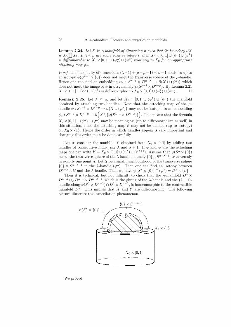
X0 × [0, 1] ∪ (ψµ) ∪ (ϕλ) may be meaningless (up to diffeomorphism as well) inthis situation, since the attaching map ψ may not be defined (up to isotopy)on X0 × 1. Hence the order in which handles appear is very important andchanging this order must be done carefully.
Let us consider the manifold Y obtained from X0 × [0, 1] by adding twohandles of consecutive index, say λ and λ + 1. If ϕ and ψ are the attachingmaps one can write Y = X0 × [0, 1] ∪ (ϕλ) ∪ (ψλ+1). Assume that ψ(Sλ × 0)meets the transverse sphere of the λ-handle, namely 0×Sn−λ−1, transversalyin exactly one point κ. Let U be a small neighbourhood of the transverse sphere0 × Sn−λ−1 in the λ-handle (ϕλ). Then one can find an isotopy betweenDn−λ × U and the λ-handle. Then we have ψ
(Sλ × 0
)∩ (ϕλ) = Dλ × κ.
Then it is technical, but not difficult, to check that the n-manifold Dλ ×Dn−λ ∪ψ Dλ+1 ×Dn−λ−1, which is the gluing of the λ-handle and the (λ+ 1)-handle along ψ(Sλ×Dn−λ)∩Dλ×Dn−λ, is homeomorphic to the contractiblemanifold Dn. This implies that X and Y are diffeomorphic. The followingpicture illustrate this cancellation phenomenon.
rκ
X0 × [0, 1]
X0 × 1
0 × Sn−λ−1
@@
@R
ψ(Sλ × 0)
@@@
@@
@@
@@
@@
@@
@@
@@@
@@
@@
@
@@
@@@
@@
@
We proved

2.1 Morse functions and handle decompositions of manifolds 27
Lemma 2.26 (Cancellation Lemma). Let X0 be a manifold without boundary,and let Y = X0×[0, 1]∪(ϕλ)∪(ψλ+1) such that ψ(Sλ×0) meets the transversesphere of the λ-handle transversaly in exactly one point. Then X0 × [0, 1] andY are diffeomorphic.
Using this Lemma, if needed, one can change a handle decomposition andadd two handles with consecutive indexes. First choose an embedded n-diskD inX0×0. Then construct an embedding ϕ : Sλ×Dn−λ → D and an embeddingψ : Sλ+1×Dn−λ−1 → ∂
(X ∪ (ϕλ)
)such that ψ(Sλ×0) meets the transverse
sphere of the λ-handle transversally in exactly one point. According to theCancellation Lemma 2.26 the manifolds X0×[0, 1] and X0×[0, 1]∪(ϕλ)∪(ψλ+1)are diffeomorphic relatively to X0.
Let us to describe how to remove a λ-handle. The first step is to constructa (λ+ 1)-handle with a transversality condition with the λ-handle which allowscancellation. Then construct a handle of indexe λ+2 such that the two handlesof indexes λ+ 1 and λ2 are cancelling together.
Now, up to technical assumptions we are ready to eliminate a λ-handle andreplace it by a (λ+ 2)-handle as stated in the following Lemma.
First we have to fix some notations. Suppose that we have a handle decom-
position of a manifold Y = X0 × [0, 1]p1⋃i=1
(ϕ1i ) . . .
pn⋃i=1
(ϕni ), then we denote
• Y q = X0× [0, 1]p1⋃i=1
(ϕ1i ) . . .
pq⋃i=1
(ϕqi ), the manifold obtained from X0× [0, 1]
after the gluing of handles of index less or equal to q,
• ∂Y q = ∂Y q \pq+1∐i=1
ϕq+1i (Sq×
Dn−1−q)
Lemma 2.27. Let X0 be a (n−1)-manifold without boundary and 1 ≤ λ ≤ n−3.
Fix a handle decomposition of Y = X0 × [0, 1]pλ⋃i=1
(ϕλi )pλ+1⋃i=1
(ϕλ+1i ) . . .
pn⋃i=1
(ϕni ),
with no handle of index strictly less than λ.Let 1 ≤ k ≤ pλ be a fixed integer. Suppose that there exists an embedding
ψλ+1 : Sλ ×Dn−1−λ → ∂Y λ such that
1. ψλ+1
|Sλ × 0 is isotopic in ∂Y λ to an embedding ξλ+1 : Sλ×0 → ∂Y λ
which meets the transverse sphere of the handle (ϕλk) and is disjoint fromthe transverse spheres of the handles (ϕλi ) i = 1, . . . , pλ
i 6= k
2. ψλ+1
|Sλ × 0 is isotopic in ∂Y λ+1 to an embedding of Sλ into a (n−1)-
disk Dn−1 ⊂ ∂Y λ+1.
Then Y is diffeomorphic, relatively to X0, to a manifold of the shape
X0 × [0, 1]⋃
i = 1, . . . , pλi 6= k
(ϕλi )pλ+1⋃i=1
(ϕλ+1i ) ∪ (ψλ+2)
pλ+2⋃i=1
(ϕλ+2i ) . . .
pn⋃i=1
(ϕni )
28 2 h-cobordism Theorem and surgeries on manifolds
Proof. All the technical asumptions made in this Lemma allow to add first a new(λ+ 1)-handle (ψλ+1) which cancel with the handle (ϕλk), second to glue a new(λ+ 2)-handle (ψλ+2) which cancel with (ψλ+1). With the second assumptionmade in the statment, the gluing of the two handles (ψλ+1) and (ψλ+2) can bemade in a (n− 1)-disk embedded in ∂Y λ+2.
Then according to the Isotopy and Cancellation Lemmas (2.21 and 2.26) wecan find the appropriate embeddings ϕikik |k = λ+ 1, . . . , n ; ik = 1, . . . , pk togive the desired handle decomposition of a manifold which is diffeomorphic toY relatively to X0.
This Lemma will be very useful to prove the h-cobordism Theorem. But firstwe have to introduce a CW-complex associated with handle decompositions ofmanifolds. This CW-complex will allow us to compute the Whitehead torsionthat appears in the s-cobordism Theorem.
2.1.2 CW-complex and handlebodies
In this subsection, we briefly recall some elementary properties of relative CW-complexes, and then we will construct a CW-complex which is associated withthe handlebody decomposition of a manifold.
Let us denote by X(0) a set of discrete points. Let n ≥ 1 be an integer.If the set X(n−1) has been defined, then consider ψαα∈An
a set of mapsfα : Sn−1 → X(n−1). Set X(n) = X(n−1) ∪
(⋃ψαDnα
)α∈An
be the gluing of
X(n−1) and some n-dimensional disks along their boundaries ∂Dnα∼= Sn−1 with
the maps ψα.This induces a filtration
X(0) ⊂ X(1) ⊂ . . . ⊂ X(n) ⊂ . . . ,
the path components of X(n) \X(n−1) are called open n-cells, the maps ψαare called attaching maps, and the maps Ψα : Dn → X(n) induced by ψα arecalled characteristic maps.
The set X =⋃n∈N X(n) is called a CW-complex. When N is not finite, then
a set is open in X if its intersection with each X(n) is open in X(n). The letter“C” stands for “closure finite” and the letter “W” stands for “weak topology”.A set is open if its intersection with each X(n) is open in X(n).
Remark 2.28. An open n-cell is open in X(n), but usually is not an open setin X.
The image of a characteristic map is a compact subset of X, which is some-times called a closed cell, but usually is not homeomorphic to Dn.
A relative CW-complex (X,A) consists of a pair of topological spaces A ⊂ X,such that X is obtained from A by gluing λ-cells, with λ ≥ 1, as we did for CW-complexes. The associated filtration is A = X(λ−1) ⊂ X(λ) ⊂ . . . ⊂ X(n) ⊂ . . ..
Let (X,A) be a relative CW-complex. Assume that X is arcwise connected1
and set π = π1(X). Let ρ : X → X be the universal covering of X, and set
1This assumption is only made in order to avoid considerations about base points andsimplify the argument.

2.1 Morse functions and handle decompositions of manifolds 29
X(q) = ρ−1(X(q)
)and A = ρ−1(A). Then (X, A) is a relative CW-complex
with the filtration A ⊂ X(1) ⊂ . . . ⊂ X(n) ⊂ . . ..Recall that the homology of the relative CW-complex (X, A) can be com-
puted using a Z[π]-chain complex C∗(X, A). The qth Z[π]-chain module is thesingular homology Hq(X(q), X(q−1)) and the π-action is coming from the cover-ing transformations, the qth differential is then given by the composite map
Hq(X(q), X(q−1))∂q→ Hq−1(X(q−1))
iq→ Hq−1(X(q−1), X(q−2)),
where ∂q is the qth boundary map associate with the homology long exact se-quence of the pair (X(q), X(q−1)) and iq is induced by the inclusion.
One can see that if we denote by βi the image of a generator of Hq(Dq, Sq−1) ∼=Z under the map (Ψq
i , ψqi )q : Hq(Dq, Sq−1) → Cq(X, A) = Hq(X(q), X(q−1)),
then the set βii∈Aq is a Z[π]-basis for Cq(X, A). We call this basis the cellu-lar basis.
Recal that the homology of a relative CW-complex is given by the homologyof the Z[π]-chain complex we just defined, i.e.,
H∗(X,A) ∼= H∗(C∗(X,A)
).
Let M be a closed (n− 1)-manifold. Now suppose we have a handle decom-position of a manifold
Y = M × [0, 1]pλ⋃i=1
(ϕλi )pλ+1⋃i=1
(ϕλ+1i ) . . .
pn⋃i=1
(ϕni ),
where the λ-handles are attached on M × 0. We denote by Y q the manifold
Y q = M × [0, 1]pλ⋃i=1
(ϕλi )pλ+1⋃i=1
(ϕλ+1i ) . . .
pq⋃i=1
(ϕqi )
obtained from M × [0, 1] by adding handles of index less or equal to q.Let us denote M × 0 by M0. Then we construct by induction over q =
λ, . . . , n a sequence of spaces X(q) with a filtration M0 ⊂ X(λ) ⊂ . . . ⊂ X(n) = Xsuch that (X,M0) is a relative CW-complex. We define the attaching maps of therelative CW-complex (X,M ×0) using the attaching maps of the handlebodydecomposition of Y .
More precisely set fλ−1 : Y λ−1 = M × [0, 1] → X(λ−1) = M0 the projection,which is a homotopy equivalence.
Assume that, for q ≥ λ, the set X(q−1) is constructed and there existsa homotopy equivalence fq−1 : Y q−1 → X(q−1). Then define the attachingmaps fq−1 ϕqi |Sq−1 × 0 for i = 1, . . . , pq to construct Y q. Now consider the
relative CW-complex (Yq, Y q), where Yq is constructed from Y q by adding q-cells with the attaching maps
ϕqi |Sq−1 × 0
i=1,...,pq
. One can see that both
X(q) and Y q are homotopically equivalent to Yq, hence there exists a homotopyequivalence fq : Y q → X(q) such that fq|Y q−1 = fq−1.
Denote by ρ : Y → Y the universal covering of Y with π = π1(Y ) ascovering transformations group. Set Y q = ρ−1(Y q). As done before in the gen-eral context of relative CW-complexex, one can associate a Z[π]-chain complex
30 2 h-cobordism Theorem and surgeries on manifolds
C∗(Y , M0). The qth Z[π]-chain module is the singular homology Hq(Y (q), Y (q−1))and the qth differential is then given by the composite map
Hq(Y (q), Y (q−1))∂q→ Hq−1(Y (q−1))
iq→ Hq−1(Y (q−1), Y (q−2)),
where ∂q is the qth boundary map associated with the homology long exactsequence of the pair (Y (q), Y (q−1)) and iq is induced by the inclusion.
Since the maps fq : Y q → X(q) constructed before are homotopy equival-cences, then we get an isomorphism of Z[π]-chain complexes
C∗(Y , M0)Θ∼= C∗(X, M0).
Moreover each handle of index q with attaching map ϕqi for i = 1, . . . , pq deter-mines an element [ϕqi ] ∈ Cq(Y , M0). And the basis [ϕqi ]i=1,...,pq
of Cq(Y , M0)maps to the cellular basis of C∗(X, M0) under Θ.
Now we are ready to prove the h-cobordism Theorem.
2.2 h-cobordism Theorem
First let us state the h-cobordism Theorem due to Smale.
Theorem 2.29 (h-cobordism [124]). Let M1 and M2 be two closed orientedand simply connected manifolds of dimension n ≥ 5. If there exists an orientedcompact manifold W with ∂W diffeomorphic to the disjoint union of M1 and−M2, and each component of ∂W is a deformation retract of W then W isdiffeomorphic to M1 × [0, 1].
The manifold −M2 is the manifold M2 with the reversed orientation.
Remark 2.30. As an important consequence we have that the two manifoldsM1 and M2 are diffeomorphic to each other.
Remark that the inclusions Mi → W , for i = 1, 2, are homotopy equiva-lences. And the letter “h” in “h-cobordism” is for homotopy equivalence.
The h-cobordism Theorem can be reformulated a follows.
Theorem 2.31 (h-cobordism). Let M1 and M2 be two closed oriented andsimply connected manifolds of dimension n ≥ 5. If there exists an orientedcompact manifold W with ∂W diffeomorphic to the disjoint union of M1 and−M2, and H∗(W,M1) = 0 then W is diffeomorphic to M1 × [0, 1].
Remark 2.32. In the second statment of the h-cobordism Theorem it is equiv-alent to replace H∗(W,M1) = 0 by H∗(W,M2) = 0.
More precisely, when H∗(W,M1) = 0 the universal coefficient Theorem im-plies H∗(W,M1) ∼= Hom
(H∗(W,M1)
)= 0, and by Poincare duality we get
H∗(W,M2) = 0. Similarly H∗(W,M2) = 0 implies H∗(W,M1) = 0
Proof of Theorem 2.31. First remark that if M1 and M2 are both deformationretracts of W then we have H∗(W,M1) = 0, and H∗(W,M2) = 0 as well.
Second when π1(M1) = 0, π1(W,M1) = 0 and H∗(W,M1) = 0 then, ac-cording to the relative Hurewicz isomorphism Theorem (see [13]), we have
2.2 h-cobordism Theorem 31
πi(W,M1) = 0 for i ∈ N. Then one can construct a deformation retractionfrom W to M1. As explained in Remark 2.31 the nullity of H∗(W,M1) impliesH∗(W,M2) = 0, and M2 is, by the same argument, a deformation retract ofW .
The h-cobordism Theorem is crucial for the study of cobordism classes ofhigh dimensional knots. It concerns simply connected manifolds, but this con-nectivity condition is automatic for knots of dimension greater or equal to 2.
In the subsection 2.2.1 we will prove an extension to non-simply connectedmanifolds called s-cobordism theorem. Though we will not need this extensionfor the study of knot cobordism, we choose to give this proof since the core ofthe proof is the same of the proof of the h-cobordism Theorem and is essentiallymade of Smale’s lemmas .
The s-cobordism Theorem was proved by Barden in [4], by Mazur in [90]and by Stallings (who never published his proof). For additional details we referto Kervaire’s paper [64] devoted to a detailed proof of this Theorem.
2.2.1 s-cobordism Theorem
Theorem 2.33 (s-cobordism Theorem). Let M1 and M2 be two closed orientedand connected manifolds of dimension n ≥ 5, and let π = π1(M1) the funda-mental group of M1. If there exists an oriented compact manifold W with ∂Wdiffeomorphic to the disjoint union of M1 and −M2, and each component of∂W is a deformation retract of W then W is diffeomorphic to M1× [0, 1] if andonly if the Whitehead torsion τ(W,M1) ∈ Wh(π) vanishes.
To make this statement understandable we have to define briefly Whiteheadgroups and Whitehead torsion, see [131] for details.
Whitehead groups. Let π be a group, and let GL(n,Z[π]) the group ofinvertible matrices of order n on the group ring Z[π]. We denote by GL(Z[π])the set of disjoint union
⋃n∈Z
GL(n,Z[π]), it is the set of invertible matrices of
arbitrary size with entries in Z[π].Let us denote by Eni,j a n× n matrix with all entries 0 except for a 1 in the
(i, j) spot; and by ∆ni (γ) a n× n diagonal matrix with entries on the diagonal
equal to 1 except for γ in the (i, i) spot. If In denotes the identity matrixof rank n, then an elementary matrix is a matrix of the form (In + aEni,j),with a ∈ Z[π]; and let E(Z[π]) be the subgroup of GL(Z[π]) generated by theelementary matrices.
It is not difficult to show that E(Z[π]) is the commutator subgroup ofGL(Z[π]), and any subgroup of GL(Z[π]) which contains E(Z[π]) is a normalsubgroup of GL(Z[π]).
Let us consider the subgroup ±π of Z[π] of trivial units, namely
p|p ∈ π ∪ −p|p ∈ π = ±π < Z[π].
Then we define I±π to be the set
I±π =M ∈ GL(Z[π]) | M = ∆n
i (γ) with γ ∈ ±π, or M ∈ E(Z[π].
32 2 h-cobordism Theorem and surgeries on manifolds
In I±π we collected the matrices of E(Z[π]) and the matrices of the formIi 0 00 γ 00 0 Ij
with γ ∈ ±π.
Hence the group Eπ, which is generated by the matrices of I±π, is a normalsubgroup of GL(Z[π]).
Definition 2.34. The whitehead group Wh(π) is the abelian quotient groupGL(Z[π])/Eπ .
In the following we will use another definition of Wh(π), which is morecomplicated but more convenient for our purpose. On GL(Z[π]) we define anequivalence relation, denoted by R, generated by the elementary operationslisted below.
Let A be a matrix in GL(Z[π]),
1. multiply the i-th row of A from left by ±γ with γ ∈ π;
2. add the i-th row to j-th row of A;
3. change the matrix A ∈ GL(n,Z[π]) to(A 00 1
);
4. change the matrix(A 00 1
)∈ GL(n+ 1,Z[π]) to A (this is the inverse of
the previous item).
Remark 2.35. We do not use column operations in our definition, i.e., rightproduct with elementary matrices. Because if two matrices A and B are re-lated together with column and row operations, then there exist two matri-ces E1 and E2, which are product of elementary matrices, such that In =
E1
(A 00 Iq
)B−1E2. But this means that E−1
2 = E1
(A 00 Iq
)B−1, and then
In = E2E1
(A 00 Iq
)B−1. This implies that A and B are related together only
using row operations.
One can define a product on classes of matrices in GL(Z[π])/R. We denoteby [A] ∈ GL(Z[π])/R the class of a matrix A ∈ GL(Z[π]). Let [A] and [B] bein GL(Z[π])/R, then there exist two integers i and j (may be equal to 0) suchthat the two matrices A ⊕ Ii and B ⊕ Ij are invertible matrices of same rank.We define [A].[B] =
[(A⊕ Ii).(B⊕ Ij)
]. The neutral element is given by [In] for
any positive integer n. The inverse of [A] is given by [A−1]. One can prove that(GL(Z[π])/R, .) is an abelian group, and Wh(π) is the quotient GL(Z[π])/R.
Proposition 2.36. These two definitions of Whitehead groups are equivalenttogether.
See [25] for this equivalence.In the following we will denote by A both a matrix in GL(Z[π]) and its class
in Wh(π).
2.2 h-cobordism Theorem 33
Whitehead torsion. We will define the Whitehead torsion of a pair (X,Y )when both X and Y are CW-complexes such that Y is a deformation retractof X. But Whitehead torsion may be defined algebraically for acyclic chaincomplexes over a ring R under some assumptions for R, we refer to [131] and[99] for detailed expositions on Whitehead torsion.
Since the inclusion Y → X is a homotopy equivalence, then it induces anisomorphism of fundamental groups π1(Y ) ∼= π1(X) = π, provided we choosea base point in Y . Let us consider again the universal covering ρ : X → X,it induces the covering ρ|Y : Y → Y and the subcomplex Y is a deformation
retract of X. Therefore the Z[π]-chain complex C∗(X, Y ) of length n is acyclic.Recall that π acts on C∗(X, Y ), and this makes it a free chain complex overZ[π]; each Z[π]-module Cq(X, Y ) equiped with the cellular basis Bq = βii∈Aq
see § 2.1.2.
1. First assume that for all integer 0 ≤ q ≤ n the Z[π]-module Im dq is free.Since the complex is acyclic, then we have the short exact sequences
0 → Im dq → Cq(X, Y )dq→ Im dq−1 → 0.
By exactness of the last short sequences we get sections sq of dq, thenset I?q−1 = sq(Iq) the image of the basis Iq−1 of Im dq−1 under sq. Notethat, since for any distinct integers i and j the two Z[π]-modules Z[π]i
and Z[π]j are not isomorphic, then the juxtaposition of the two basis Iqand I?q−1 is a basis of Cq(X, Y ). Set TIqI?
q−1→Bqthe transition matrix
from IqI?q−1 to Bq.The following product matrix
τ =n∏i=0
T(−1)i+1
IqI?q−1→Bq
is invertible.
Moreover one can prove that its class in Wh(π) does not depend on thechoices of the basis and is invariant under cellular subdivisions. Accordingto these facts when for all integer 0 ≤ q ≤ n the Z[π]-module Im dq arefree, then we define the torsion of the complex C∗(X, Y ) to be the classof τ in Wh(π).
2. When the Z[π]-module Im dq are not free we have the following Lemma
Lemma 2.37. For all integers 0 ≤ q ≤ n there exists a free Z[π]-moduleFq such that the Z[π]-module Im dq ⊕ Fq is free.
Proof. Note that Im d0 = C0(X, Y ) is free.
We will prove the property by induction on q. Assume there exists aninteger k ≥ 0 for which there exists a free Z[π]-module Fk such that theZ[π]-module Im dk ⊕ Fk is free.
Since the Z[π]-chain complex C∗(X, Y ) of length n is acyclic, then we havethe following short exact sequence
0 → Im dk+1 → Ck(X, Y )⊕ Fkdk⊕Id−→ Im dk ⊕ Fk → 0.

34 2 h-cobordism Theorem and surgeries on manifolds
The last Z[π]-module is free, hence there exists a section σk for dk ⊕ Id.The Z[π]-module σq(Im dk ⊕ Fk) is free, and Im dk+1 ⊕ σq(Im dk ⊕ Fk) =Ck(X, Y )⊕ Fk as well.
Let us denote by Cq∗(F ) the free based acyclic Z[π]-chain complex associ-ated with a free based Z[π]-module F , which has dq : F → F as the onlynon-trivial differential
. . .→ 0 → Fdq→ F → 0 → . . . .
Define a new Z[π]-chain complex C∗(X, Y )⊕n
k=0 Ck∗ (Fk). Since in this
free acyclic Z[π]-chain complex the image of the differential are some freeZ[π]-modules, then we can compute its torsion as just made before. Onecan prove that the torsion of this complex does not depend on the choicesmade on the free Z[π]-modules Fq for q = 0, . . . , n.
We define the torsion τ(X,Y ) to be the torsion of the Z[π]-chain complexC∗(X, Y )
⊕nk=0 C
k∗ (Fk).
Come back to the statement of the s-cobordism Theorem. Assume that W isan oriented compact manifold with boundary ∂W ∼= M1
∐−M2, such that both
M1 and M2 are deformation retracts of W . To a handlebody decomposition
W = M1 × [0, 1]p0⋃i=1
(ϕ0i ) . . .
pλ⋃i=1
(ϕλi ) . . .pn⋃i=1
(ϕni ),
one can associate first a Z[π]-chain complex C∗(W , M1) and second a relativeCW-complex (X, M1) such that the Z[π]-chain complex C∗(X, M1) is isomorphicto C∗(W , M1).
Since M1 is a deformation retract of W , in the relative CW complex (X, M1)we have that M1 is a deformation retract of X as well. Hence τ(X, M1) is welldefined, and the torsion τ(W,M1) is by definition equal to the torsion τ(X, M1).
Simple homotopy equivalences. When the map f : E → F is a homotopyequivalence between CW-complexes, then F is a deformation retract of themapping cylinder
Mf =(X × [0, 1]
) ∐Y/(x, 1) ∼ f(x)
of f .We define the Whitehead torsion of f , denoted by τ(f) ∈ Wh
(π1(Y )
), to
be the image of the torsion τ(Mf , Y ) ∈ Wh(π1(Mf )
)in Wh
(π1(Y )
)under the
isomorphism between Wh(π1(Mf )
) ∼=→ Wh(π1(Y )
)induced by the isomorphism
π1(Mf )∼=→ π1(Y ).
This torsion is well defined, and when two cellular homotopy equivalencesbetween two CW-complexes are homotopic the torsion are equal.
Definition 2.38. We say that a homotopy equivalence f : X → Y of finiteCW-complexes is simple if the torsion τ(f) vanishes in Wh
(π1(Y )
).
This definition extend to homotopy equivalences between smooth manifolds.
2.2 h-cobordism Theorem 35
Remark 2.39. In the statement of the s-cobordism Theorem the inclusionsMi → W are simple homotopy equivalences. The letter “s” in ”s-cobordism”refer to simple homotopy equivalence.
Proof of the s-cobordism Theorem. To prove the s-cobordism Theoremwe need some technical Lemmas. There exists many written proofs of thesecrucial Lemmas in the literature, see Luck [85] and Kervaire [64].
Let us fix some notations. In the following we will consider handle decom-positions of a manifold W which has M1
∐M2 has boundary.
W = M1 × [0, 1]p0⋃i=1
(ϕ0i ) . . .
pλ⋃i=1
(ϕλi ) . . .pn⋃i=1
(ϕni ).
Then we will denote
Wλ = M1 × [0, 1]p0⋃i=1
(ϕ0i ) . . .
pλ⋃i=1
(ϕλi )
the manifold obtained from M1× [0, 1] after the gluing of handles of indexesless or equal to λ, and
∂Wλ+ = ∂Wλ \
(pλ+1∐i=1
ϕλ+1i (Sλ×
Dn−1−λ)
∐M × 0
)the upper boundary of Wλ without the gluing sets of handles of index λ+ 1.
Lemma 2.40. Let W be an oriented compact n-manifold with n ≥ 6 and ∂Wis diffeomorphic to the disjoint union of two compact (n− 1)-manifolds M1 andM2. Suppose that each component of ∂W is a deformation retract of W , thenW is diffeomorphic to M1 × [0, 1]
⋃p2i=1(ϕ
2i ) . . .
⋃pn
i=1(ϕni ) relatively to M1.
Proof. Let M1 × [0, 1]⋃p0i=1(ϕ
0i ) . . .
⋃pn
i=1(ϕni ) be a handle decomposition of W .
To prove this Lemma we have to show that we can remove the handle of indexes0 and 1.
Recall that to add a 0-handle we make the disjoint union with a n-disk.But since W is connected there exists almost one 1-handle joining M1 × [0, 1]to this n-disk. Up to isotopy all the gluing sets of 1-handles, which are not inthe 0-handles, are in M1 × 1, hence the order of attaching 1-handles is notimportant. So if (ϕ0
1) is the first 0-handle, one can assume that the 1-handle (ϕ11)
is joining M1× [0, 1] to (ϕ01). But the gluing of (ϕ1
1) with (ϕ01) is homeomorphic
to a n-disk since we only attach one connected component of the boundary ofthe 1-handle to the 0-handle. These two handles (ϕ1
1) and (ϕ01) are cancelling
together, so we can remove the 0-handle (ϕ01) and the 1-handle (ϕ1
1). Finallyone may assume that there is no 0-handle.
The handle decomposition of W became M1×[0, 1]⋃p1−p0i=1 (ϕ1
i ) . . .⋃pn
i=1(ϕni ).
Since ∂W 0+ consists only in M × 1 with 2 p1 disks of dimension (n − 1)
removed, then π1(∂W 0+) = π1(M × 1). Moreover M1 × 1 is a deformation
retract of W , so π1(∂W 0+) maps surjectively onto π1(W ). Let φ1
1 : D1×Dn−1 →W 1 the embedding of the 1-handle (ϕ1
1) . Consider now [σ] ∈ π1(W 1) given bythe homotopy class of σ = φ1
1
(D1 × 0
)∪ γϕ1
1(S0×0) the gluing , along their
36 2 h-cobordism Theorem and surgeries on manifolds
boundary of the core the 1-handle and a path γ, which join in ∂W 0+ the two
points of ϕ11(S
0 × 0). By construction [σ] is in not equal to 0 in π1(W 1); butsince π1(W ) ∼= π1(M1), then [σ] must be 0 in π1(W ). This means that σ isnullhomotopic in W . Because of the dimensions, one can find some attachingmaps ϕ′2i i=1,...,p2 isotopic to ϕ2
i i=1,...,p2 such that for all i = 1, . . . , p2 theimages of ϕ′2i do not meet the loop σ. Hence one can construct an embeddingφ : S1 → ∂W 1 such that
[φ(S1)
]= [σ] and φ(S1) meets the transverse sphere
of (ϕ11) transversally in exactly one point. Since σ is nullhomotopic in W , then
φ is nullhomotopic in W and in ∂W 2 as well. This means that the image of φbounds an immersed 2-disk, and twice the dimension of this disk is strictly lessthan the dimension of ∂W 2, which is 5. According to Whintney’s embeddingTheorem, this homotopy can be realized with an embedding of a 2-disk in ∂W 2.This means that one can extend φ to an embedding Φ : S1 × Dn−1 → ∂W 2
which is isotopic to a trivial embedding in ∂W 2. By construction Φ fullfilsthe hypothesis of Lemma 2.27, so we can eliminate the first 1-handle in thedecomposition of W . By induction we get the desired decomposition
W ∼= M1 × [0, 1]p2⋃i=1
(ϕ2i )
p′3⋃i=1
(ϕ3i ) . . .
pn⋃i=1
(ϕni )
Remark 2.41. In the proof we strongly used the assumption n ≥ 6 to smoothimmersed disks to embedded disks.
As a consequence of this Lemma one can give a description of the Z[π]-chaincomplex C∗(W , M1) in term of homotopy groups, see § 2.1.2 for the definitionof this complex, where we have identified M1 × 0 to M1, the manifold W isthe universal covering of W and π = π1(W ).
First we fix a base point in M1 × 0 and a lift of that point in ρ−1(W ), allthe homotopy groups will be considered with respect to these base points. Nowwe define the Z[π]-chain complex
π∗(W ∗,W ∗−1) =
0 if q ≤ 1,πq(W q,W q−1) if q ≥ 2.
The differentials are given by the composite maps
πq(W q,W q−1)∂q→ πq−1(W q−1)
iq−1→ πq−1(W q−1,W q−2)
where ∂q is a boundary operator, and iq−1 is induced by the inclusion.For all q ≥ 1 the group π1(W q−1) is trivial, then the relative Hurewicz
homeomorphism πq(W q, W q−1) → Hq(W q, W q−1) is an isomorphism. Moreoverthe covering maps ρq : W q → W q induce the isomorphisms πq(W q, W q−1) ∼=πq(W q,W q−1). Finally we get an isomorphism of Z[π]-chain complexes
C∗(W , M1) ∼= π∗(W ∗,W ∗−1).
Each basis element [ϕqi ] ∈ Cq(W , M1), associate with the attaching maps ofthe handles, can be considered as an element of πq(W q,W q−1) with this iso-morphism. It corresponds to the element given by the homotopy class of themapping
(Dq × 0, ϕq(Sq−1 × 0
)→ (W q,W q−1).
2.2 h-cobordism Theorem 37
In the following Lemma we give conditions which ensure that the embeddingof a sphere meets suitably the transverse spheres of a handle decomposition.
Lemma 2.42. Let W be a compact n-manifold with n ≥ 6 and ∂W is diffeo-morphic to the disjoint union of two compact (n − 1)-manifolds M1 and M2.Suppose that W is diffeomorphic to M1 × [0, 1]
⋃p2i=1(ϕ
2i ) . . .
⋃pn
i=1(ϕni ) relatively
M1.Fix λ ∈ 1, . . . , n − 3 and k ∈ 1, . . . , pλ. Let f : Sλ → ∂Wλ
+ be anembedding. Then the following are equivalent
1. There exists an embedding g : Sλ → ∂Wλ+ isotopic to f which meets the
transverse spheres of the λ-handle (ϕλk) transversally in exactly one pointand is disjoint from the transverse spheres of the λ-handles
(ϕλi )
i 6=k,
2. For any lift f : Sλ → Wλ of f under ρ|Wλ ; if [f ] denotes the image of f
under the composite map πλ(Wλ) → πλ(Wλ, Wλ−1) → Hλ(Wλ, Wλ−1),then there exists γ ∈ π such that [f ] = ±γ[ϕλk ].
Proof. When the transversality conditions of the first statement are fulfilled,the second follows easily.
Let us explain the converse. Because of dimensions the image of f meets theset of transverse spheres of the λ-handles only in a finite number of points, set
Im f⋂
0 × Sn−λ−1i
i=1,...,pλ
=xi,1, . . . , xi,ni
i=1,...,pλ
.
Fix ∗ ∈ Im f a base point in W , and in each transverse sphere 0×Sn−λ−1i
fix a base point ∗i, for i = 1, . . . , pλ, such that ∗i 6∈xi,1, . . . , xi,ni
i=1,...,pλ
.
Now let ci,j : [0, 1] → Sλ be a path such that for all (i, j) ∈ 1, . . . , pλ ×1, . . . , ni we have fci,j(0) = ∗ and fci,j(1) = xi,j . Let bi,j : [0, 1] →Wλ be apath such that for all (i, j) ∈ 1, . . . , pλ×1, . . . , ni we have bi,j(0) = xi,j andbi,j(1) = ∗i. And let ai : [0, 1] →Wλ be a path such that for all i ∈ 1, . . . , pλwe have ai(0) = ∗i and ai(1) = ∗.
Now let li,j a loop base in ∗, which is the composite path of f(ci,j), bi,j andai. if we denote by γi,j the homotopy class of li,j in π = π1(W, ∗), then we have
[f ] =pλ∑i=1
ni∑j=1
εi,j γi,j [ϕλi ]
where εi,j = ±1.We assume that there exists γ ∈ Z[π] such that [f ] = ±γ[ϕλk ], but since the
set[ϕλi ]
i=1,...,pλ
is a basis of Hλ(Wλ, Wλ−1) then, for i 6= k, we can associatethe elements of
xi,1, . . . , xi,ni
i=1,...,pλ
by pairs such that for each pair, say(xi,j1 , xi,j2), we have εi,j1 εi,j2 = −1. This means that the loop, which is thecomposite path of f(ci,j1), bi,j1 , the inverse of bi,j2 and the inverse of f(ci,j2) isnullhomotopic in ∂Wλ
+.Now, since n ≥ 6, then one can apply the Whitney trick (see [141]) to modify
f with an isotopy, and get new embedding of Sλ in ∂Wλ+ with the two inter-
section points xi,j1 and xi,j2 removed and no change to the other intersectionpoints with the transverse spheres.

38 2 h-cobordism Theorem and surgeries on manifolds
By induction we get the first statement with γ = ±nk∑j=1
εk,j γk,j .
Lemma 2.43. Let f : Sλ → ∂Wλ+ be an embedding , and let xjj=1,...,pλ+1 be
a set of elements of Z[π].An embedding g : Sλ → ∂Wλ
+ is isotopic to f if and only if to each liftf : Sλ → Wλ of f under ρ|Wλ one can find a lift g : Sλ → Wλ of g such that
in Hλ(Wλ,Wλ−1) we have
[g] = [f ] +pλ+1∑j=1
xj dλ+1[ϕλ+1j ]
where dλ+1 is the (λ+ 1)-differential of the complex C∗(W , M1).
This Lemma is more or less proved in Smale’s work [124], for a proof see [64]or [85].
Lemma 2.44. Let W be an oriented compact n-manifold with n ≥ 6 and ∂Wis diffeomorphic to the disjoint union of two compact (n− 1)-manifolds M1 andM2. Suppose that each component of ∂W is a deformation retract of W , thenfor any λ ∈ 2, . . . , n− 3 there exists a handlebody decomposition of W of theform
M1 × [0, 1]pλ⋃i=1
(ϕλi )pλ+1⋃i=1
(ϕλ+1i ).
Proof. We saw that handles of indexes 0 and 1 can be removed so we start witha handle decomposition for W of the form
W ∼= M1 × [0, 1]p2⋃i=1
(ϕ2i ) . . .
pn⋃i=1
(ϕni ).
Now we will show that we can decrease pq by one provided that pr = 0 forr ≤ q − 1 and q ≤ n− 3.
Start with a decomposition W ∼= M1× [0, 1]⋃pq
i=1(ϕqi ) . . .
⋃pn
i=1(ϕni ). As done
before the trick is to attach a new (q+1)-handle, which cancel with (ϕq1), and anew (q + 2)-handle such that the two new handles cancel together. To do thatwe will use Lemma 2.27.
Let Ψq+1 : Sq+1 ×Dn−q−1 → ∂W q+ be an embedding such that its image is
included in a n-disk Dn ⊂ ∂W q+.
Since the inclusion M1 → W is a homotopy equivalence, then the Z[π]-chain complex C∗(W , M1) is acyclic. But we assume that there is no k-handlewith k ≤ q − 1 in the handle decomposition for W , hence the the Z[π]-moduleCq−1(W , M1) = Hq−1(W q−1, W q−2) is trivial. So the (q + 1)-differential of thecomplex C∗(W , M1), namely dq+1 : Cq+1(W , M1) → Cq(W , M1), is surjective.This implies that there exists a set xki=1,...,pq+1 of elements in Z[π], such that
Hq(W q, W q−1) 3 [ϕq1] =pq+1∑i=1
xi dq+1
([ϕq+1i ]
).
2.2 h-cobordism Theorem 39
According to Lemma 2.43, one can find an embedding ψq+1 : Sq+1×Dn−q−1 →∂W q+1
+ , which is isotopic to Ψq+1 in ∂W q+1+ , such that
[ψq+1|Sq×0] = [Ψq+1
|Sq×0] +pq+1∑i=1
xi dq+1
([ϕq+1i ]
).
But [ψq+1|Sq×0] = [ϕq1] since [Ψq+1
|Sq×0] is nullhomotopic in ∂W q+1+ . Moreover,
according to Lemma 2.42 the embedding ψq+1|Sq×0 is isotopic in ∂W q+1
+ to an
embbeding Sq → ∂W q+1+ which meets the transverse sphere of (ϕq1) transversally
exactly in one point and do not meet the transverse spheres of the other q-handles.
We can apply Lemma 2.27 to find a new handle decomposition
W ∼= M1 × [0, 1]pq⋃i=2
(ϕqi )pq+1⋃i=2
(ϕq+1i ) ∪ (ψq+2)
pq+2⋃i=2
(ϕq+2i ) . . .
pn⋃i=1
(ϕni ),
and the number of q-handle decreased by one. By induction we can remove allq-handles.
Now using the dual handle decomposition for W , i.e., the handle decom-position associated with the Morse function −f instead of f which start withM2 × [0, 1]; we have the following decomposition
W ∼= M2 × [0, 1]p0⋃i=1
(φni ) . . .pλ⋃i=1
(φn−λi ) . . .pn⋃i=1
(φ0i ).
As just explained before one can remove handles of indexes less or equal ton− λ− 2 in this decomposition, and
W ∼= M2 × [0, 1]p0⋃i=1
(φni ) . . .pλ+1⋃i=1
(φn−λ−1i ).
If we take again the dual handle decomposition of the last one, then one canfind a handle decomposition for W of the form
W ∼= M1 × [0, 1]p0⋃i=1
(Φ0i ) . . .
pλ+1⋃i=1
(Φλ+1i ).
Now we remove all handles of indexes less or equal to λ − 1 in the lastdecomposition and we get the desired result
W ∼= M1 × [0, 1]pλ⋃i=1
(ϕλi )pλ+1⋃i=1
(ϕλ+1i ).
We are ready to finish the proof of the s-cobordism Theorem.
Proof of s-cobordism Theorem. With the previous Lemma 2.44 we can assumethat the manifold W admits a handle decomposition of the form
W ∼= M1 × [0, 1]p⋃i=1
(ϕλi )p⋃i=1
(ϕλ+1i ).

40 2 h-cobordism Theorem and surgeries on manifolds
The number of handle is the same since we assume that both M1 and M2 aredeformation retracts of W .
The acyclic Z[π]-chain complex C∗(W , M1) has only one differential whichis non zero, namely dλ+1 : Hλ+1(Wλ+1, Wλ) → Hλ(Wλ, Wλ−1). Let D be thematrix of the isomorphism dλ+1 with respect to the basis [ϕλ+1
i ]i=1,...,p ofCλ+1(W , M1) = Hλ+1(Wλ+1, Wλ) and the basis [ϕλi ]i=1,...,p of Cλ(W , M1) =Hλ(Wλ, Wλ−1). The entries di,j ∈ Z[π] of the matrix D, for i, j = 1, . . . , p, aredefined by the equations
dλ+1
([ϕλ+1i ]
)=
p∑j=1
di,j [ϕλj ].
By definition, the Whitehead torsion τ(W,M1) is given by the class of thematrix D in Wh(π).
Let us give the geometrical interpretation of the four elementary operationswhich generate the Whitehead group described in Definition 2.34 and Proposi-tion 2.36, when these operations are made on the matrix D we just defined.
1. The multiplication of the k-th row of D by ±γ with γ ∈ Z[π] correspond tothe modification of the lift in Wλ+1 of ϕλk . But according to Lemma 2.43this corresponds to the gluing of a new λ-handle (ϕ′λk ) instead of (ϕλk).The resulting manifold is diffeomorphic to W .
2. Similarly to the previous item, the addition to the k-th row of the j-throw of D can be realized by the gluing of a new λ-handle which is isotopicto (ϕλk).
3. This operation corresponds to the gluing of a new λ-handle (ψλ) and anew (λ+ 1)-handle (ψλ+1) in a n-disk of ∂Wλ+1
+ , such that these handlesare cancelling together.
4. This operation is the converse of the previous one, when we do it wejust remove to handles, which are cancelling together, from the handledecomposition of W .
Since all of the modifications on the matrix D correspond to modifications ofthe handle decomposition of W which do not change W up to diffeomorphism,then we see that the Whitehead torsion τ(W,M1) vanishes if and only if Wadmits a handle decomposition in which all handles can be removed, and thenW ∼= M1 × [0, 1].
Proposition 2.45. The s-cobordism Theorem implies the h-cobordism Theo-rem.
Proof. Recall that any invertible matrix over the integers can be reduced byelementary operations to the identity matrix. So all the matrices in GL(Z)are equivalent in Wh(Z) which is trivial. When the manifolds M1 and M2 aresimply connected, then Wh(π) = 0 and the s-cobordism Theorem implies theh-cobordism Theorem.

2.3 Surgery on manifolds 41
2.2.2 The relative case
The notion of relative h-cobordism was introduced by Heafliger [45].
Definition 2.46. Two pairs (M1, V1) and (M2, V2) of manifolds with Vi ⊂Mi
for i = 1, 2 are h-cobordant if there exist a pair of manifold (M,V ) with V ⊂Msuch that ∂M = M1 −M2, ∂V = V1 − V2 and the inclusion Mi →M , Vi → Vare homotopy equivalences for i = 1, 2.
Then the h-cobordism and s-cobordism theorems can be extended to therelative case.
2.3 Surgery on manifolds
In this section we describe modifications on manifolds called surgeries. We in-troduce them now since they are very similar to handle gluing. In handlebodydecompositions of manifolds, we attach handles in order to give some descrip-tions of the manifolds.
Start with a n-manifold X, and let ψ : Sk ×Dn−k → X be an embeddingfor 0 < k < n. Set Y be the manifold obtained from X as follows
Y = X \(ψ(Sk ×Dn−k) ∪∂ (
Dk+1 × Sn−k−1),
where the gluing is given by the identification of boundaries.
Definition 2.47. We say that Y is obtained from X after a surgery on ψ(Sk).When the manifold X is embedded in a manifold W , if there exist an embed-
ding φ : Dk+1 × Sn−k−1 → W \(ψ(Sk×
Dn−k)
)such that ψ(Sk × Sn−k−1) =
ψ(Sk × Sn−k−1), then we say that the manifold
Y = X \(ψ(Sk ×Dn−k) ∪∂ φ(Dk+1 × Sn−k−1),
is obtained from X after an embedded surgery on ψ(Sk).
In fact surgeries can be described with handles gluing. The manifold Yconstructed by surgery on ψ(Sk) can be viewed as the upper boundary of
X × [0, 1] ∪ (ψk+1),
as depicted bellow
ψ(Sk ×Dn−k)
X
Y
X × [0, 1]
(ψk+1)
42 2 h-cobordism Theorem and surgeries on manifolds
Modifications of manifolds with surgeries change homology groups. Moreprecisely a suregry on ψ(Sk) in a manifold X gives a manifold Y in which thehomology class of ψ(Sk) is zero. So if ψ(Sk) is a n-dimensional chain wichrepresent a non trivial homology class in X, then the rank of the kth homologygroup of Y may not be equal to those ofX. Moreover if ψ(Sk) is a n-dimensionalchain wich represent a trivial homology class in X then a surgery on ψ(Sk) mustadd some homology class of dimension not equal to n.
Anyway, using Mayer-Vietoris exact sequences associated with decomposi-tion of manifolds like
X \(ψ(Sk ×Dn−k) ∪∂ (
Dk+1 × Sn−k−1),
one can compute exactly how a surgery modifies the homology of X.We will combine surgeries and h-cobordism Theorem to construct cobordism
of knots. More precisley, to prove that two knots K0 and K1 are cobordant, weneed to find a manifold X such that ∂X = K0
∐K1 and X ∼= K0 × [0, 1]. A
way to do that is to start with a manifold Z such that ∂Z = K0
∐K1 and do
some surgeries on Z to get a manifold X with H∗(X,K0) = 0 and then applythe h-cobordism Theorem to get X ∼= K0 × [0, 1].
Chapter 3
Spherical knots
”Die Mathematiker sind eine Art Franzosen:Redet man zu ihnen, so bersetzen sie es in ihre
Sprache, und dann ist es alsbald etwas anderes.”J.W. von Goethe,
- Maximen und Reflexionen
In this chapter, we consider the case of spherical knots. In the sixties,Kervaire and Levine gave classifications of spherical knots up to cobordism, wewill recall some of their results in the following.
Unless specified all knots in this chapter are simple spherical (2n−1)-knots.
3.1 Alexander polynomial
3.2 S-equivalence
The Seifert form is the main tool to study cobordisms of odd dimensional spher-ical knots. Since spherical knots are not in general fibered, then there existsmany distinct Seifert manifolds for a given spherical knot. Before going futher,the first step is to know what happen on Seifert forms when we change theSeifert manifolds associated with a spherical knot. In [82] Levine described thepossible modifications on Seifert forms of a spherical simple knot correspondingto alterations of Seifert manifolds.
For a given (2n− 1)-knot K embedded in S2n+1 let us consider two Seifertmanifolds V1 and V2 associated with K. One can suppose that Vi × i isembedded in S2n+1 × i → S2n+1 × [0, 1] for i = 0, 1. We denote by Ai theSeifert form associated with Vi, and by Si = Ai+(−1)nAi the intersection formassociated with Vi for i = 0, 1.
With similar arguments as those used to proved that every knot bounds anembedded Seifert manifold, ons can see that there is no obstruction to constructan embedded submanifoldW of S2n+1×[0, 1] such that ∂W = V0∪K×[0, 1]∪V1.Then the handle decomposition associated with a Morse function f : W → [0, 1]show that V0 and V1 are related each other by embedded surgeries.
Remark 3.1. The manifold W is very usefull to construct submodules onwhich the Seiferts forms vanishe. More precisely, when two n-cycle α and β inH(V0)⊕H(V1) are null-homologous in Hn(W ) then A0 ⊕−A1(x, y) = 0.
To prove the last equality, remark that the positive direction of the normalbundle of V0
∐V1 in S2n+1 extend to a positive direction of the normal bundle
of W in S2n+1× [0, 1]. Set ξ and η some (n+1)-chains in W such that [∂ξ] = xand [∂η] = y and ξ+W
the chain ξ pushed out W in the positive normal directionin S2n+1× [0, 1]. Since the two chains ξ+W
and η do not intersect together, then
A0 ⊕−A1(x, y) = lS2n+1
((∂ξ)+, (∂η)
),
A0 ⊕−A1(x, y) = IS2n+1×[0,1](ξ+W, η),
A0 ⊕−A1(x, y) = 0.
44 3 Spherical knots
When the critical points of f are not of index n nor n+1 then the associatedsurgeries do not modify the homolgy groups Hn(V0) and Hn(V1); hence thesemodifications do not affect the Seifert forms associated with V0 and V1.
Since the critical points of f are isolated, then it suffices to consider thecase where f has only one critical point. First, suppose that the critical pointis of index n. The corresponding surgery means that we attach a n-handleto V0. More precisely, remove Dn+1 × Sn−1 and glue Sn × Dn along thenew boundary. Elementary computation with Mayer-Vietoris sequences giveHn(W,V0) ∼= Hn+1(W,V1) ∼= Z and Hn(W,V1) ∼= H(W,V0) = 0. Let a be theimage in H(V1) of the generator of H(W,V1). If a has a finite order, then Seifertforms associated with V0 and V1 are isomorphic since they are defined modulotorsion.
If a has infinte order, then it is a multiple of a primitive element a0 of H(V1).Moreover there exists b0 in H(V1) such that S1(a0, b0) = 1. Since rk
(H(V1)
)=
rk(H(V0)
)+2 one can take (c1, . . . , ck) in H(V1) such that (a0, b0, c1, . . . , ck) is a
basis of H(V1) and (c1, . . . , ck) are homologous to a basis (d1, . . . , dk) of H(V0).There exist a (n+1)-chain Γi in W such that ∂Γ is a n-chain which represent
the cycle di−ci for i = 1, . . . , k. Then for all i, j in 1, . . . , k we have A0(di, dj)−A1(ci, cj) is the intersection number of Γj and the translate of Γi off W in thepositive normal direction of W in S2n+1× [0, 1]. Since this intersection numberis zero then for all i, j in 1, . . . , k we have A0(di, dj) = A1(ci, cj). By definitiona is null-homologous in W , hence we get A1(a, ci) = A1(ci, a) = A1(a, a) = 0for i = 1, . . . , k. Thus we have A1(a0, ci) = A1(ci, a0) = A1(a0, a0) = 0. If A0
(resp. A1) is the matrix of A0 (resp. A1) with respect to the basis (d1, . . . , dk)(resp. (c1, . . . , ck, a0, b0)), then
A1 =
A0 O νOT 0 wµT z v
,
where O is a column vector whose entries are all 0, and ν, µ are column vectorof integers.
Since S1(a0, b0) = 1 then we have w+(−1)nz = 1. Recall that the Alexanderpolynomial of K is well defined up to a unit in Z[t, t−1]. If we denote by ∆Ai
(t)the Alexdander polynomial associated with Ai for i = 0, 1, then ∆A1(t) =(tw+(−1)nz)(tz+(−1)nw)∆A0(t). So w or z must be 0, if w = 0 then one canmodify the vectors of the basis (c1, . . . , ck, a0, b0) to get
A1 =
A0 O Oµ′T 0 0
OT 1 0
.
Hence we define the enlargement A′ of a square integral matrix A as follows:
A′ =
A O OαT 0 0OT 1 0
or
A β OOT 0 1OT 0 0
,
where O is a column vector whose entries are all 0, and, α and β are columnvectors of integers. In this case, we also call A a reduction of A′.

3.2 S-equivalence 45
Definition 3.2. Two square integral matrices are said to be S-equivalent ifthey are related each other by enlargement and reduction operations togetherwith the congruence. We also say that two integral bilinear forms defined on freeZ-modules of finite rank are S-equivalent if so are their matrix representatives.
This equivalence relation characterize isotopy classes of spherical simple(2n − 1)-knots with n ≥ 2 as stated in the following Theorem proved byLevine [82].
Theorem 3.3 ([82]). For n ≥ 2, two spherical simple (2n−1)-knots are isotopicif and only if they have S-equivalent Seifert forms.
We will need the two following Lemmas for the proof.
Lemma 3.4. Let K be a simple spherical (2n− 1)-knot, and let A be a Seifertmatrix associated with a (n − 1)-connected Seifert manifold for K. If Bis anenlargement of A then B is a Seifert matrix associated with a (n− 1)-connectedSeifert manifold for K as well.
Proof. By Alexander duality
Lemma 3.5. If n ≥ 2, then two simple spherical (2n − 1)-knots admittingidentical Seifert matrices, associated with (n − 1)-connected Seifert manifoldsfor K, are isotopic.
We refer to [82] p.191 for a proof of this Lemma, which is based on handledecompositions for Seifert manifolds. Though the result is valid for all n ≥ 2,we have to mention that special arguments must be used when n = 2.
When K is a spherical (2n− 1)-knot with Seifert manifold F , then the longexact sequence in homology of (F,K) induces the exact short sequence
0 → Hn(F ) S∗→ Hn(F,K) → 0.
Morever when K is simple then Hn(F,K) is isomorphic to HomZ(Hn(F ),Z);and if we equip Hn(F,K) with the dual basis of the one choosed for Hn(F ) thenthe matrix of S∗ is A+ (−1)n tA, where A is the Seifert matrix associated withF . So in that case we have det
(A+ (−1)n tA
)= ±1. The converse is also true
as stated bellow.
Proposition 3.6 ([82]). Let n be an integer greater or equal to 2, and let A bean integral square matrix such that A+ (−1)n tA is unimodular. If n 6= 2, thereexists a simple spherical (2n − 1)-knot with Seifert matrix A; if n = 2, thereexists a simple spherical 3-knot with Seifert matrix S-equivalent to A.
Proof of Theorem 3.3. First suppose that two simple spherical (2n − 1)-knotsK0 and K1 are isotopic, then using the same argument to compute modificationson Seifert forms corresponding to alterations of Seifert manifolds, we see thattheir Seifert forms are S-equivalent.
For the converse, star with two simple spherical (2n− 1)-knots, denoted byK and K ′, with S-equivalent Seifert forms. Then there exist a finite sequenceof matrices A1, . . . , Ak such that A1 = A is a Seifert matrix for K, Ak = A′
is a Seifert matrix for K ′ and for all i = 1, . . . , k − 1 the matrix Ai+1 is anenlargement or a reduction of Ai up to congruence.
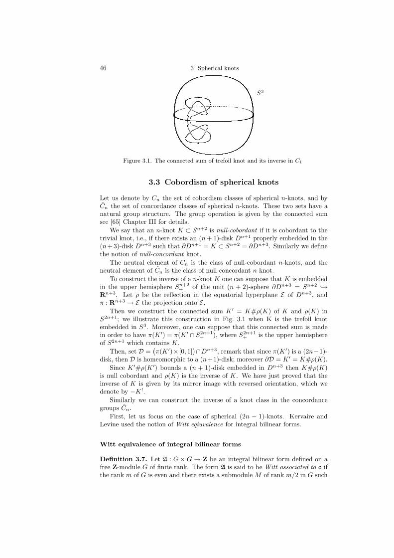
46 3 Spherical knots
-
S3
Figure 3.1. The connected sum of trefoil knot and its inverse in C1
3.3 Cobordism of spherical knots
Let us denote by Cn the set of cobordism classes of spherical n-knots, and byCn the set of concordance classes of spherical n-knots. These two sets have anatural group structure. The group operation is given by the connected sumsee [65] Chapter III for details.
We say that an n-knot K ⊂ Sn+2 is null-cobordant if it is cobordant to thetrivial knot, i.e., if there exists an (n+ 1)-disk Dn+1 properly embedded in the(n+3)-disk Dn+3 such that ∂Dn+1 = K ⊂ Sn+2 = ∂Dn+3. Similarly we definethe notion of null-concordant knot.
The neutral element of Cn is the class of null-cobordant n-knots, and theneutral element of Cn is the class of null-concordant n-knot.
To construct the inverse of a n-knot K one can suppose that K is embeddedin the upper hemisphere Sn+2
+ of the unit (n + 2)-sphere ∂Dn+3 = Sn+2 →Rn+3. Let ρ be the reflection in the equatorial hyperplane E of Dn+3, andπ : Rn+3 → E the projection onto E .
Then we construct the connected sum K ′ = K#ρ(K) of K and ρ(K) inS2n+1; we illustrate this construction in Fig. 3.1 when K is the trefoil knotembedded in S3. Moreover, one can suppose that this connected sum is madein order to have π(K ′) = π(K ′ ∩ S2n+1
+ ), where S2n+1+ is the upper hemisphere
of S2n+1 which contains K.Then, set D =
(π(K ′)× [0, 1]
)∩Dn+3, remark that since π(K ′) is a (2n−1)-
disk, then D is homeomorphic to a (n+1)-disk; moreover ∂D = K ′ = K#ρ(K).Since K ′#ρ(K ′) bounds a (n + 1)-disk embedded in Dn+3 then K#ρ(K)
is null cobordant and ρ(K) is the inverse of K. We have just proved that theinverse of K is given by its mirror image with reversed orientation, which wedenote by −K !.
Similarly we can construct the inverse of a knot class in the concordancegroups Cn.
First, let us focus on the case of spherical (2n − 1)-knots. Kervaire andLevine used the notion of Witt eqiuvalence for integral bilinear forms.
Witt equivalence of integral bilinear forms
Definition 3.7. Let A : G × G → Z be an integral bilinear form defined on afree Z-module G of finite rank. The form A is said to be Witt associated to 0 ifthe rank m of G is even and there exists a submodule M of rank m/2 in G such

3.3 Cobordism of spherical knots 47
that M is a direct summand of G and A vanishes on M . Such a submodule Mis called a metabolizer for A.
The following theorem was proved by Levine [80] and Kervaire [66].
Theorem 3.8. For n ≥ 2, a spherical (2n − 1)-knot is null-cobordant if andonly if its Seifert form is Witt associated to 0.
Proof.
For two spherical (2n − 1)-knots K0 and K1 with Seifert forms A0 andA1 respectively, the oriented connected sum K = K0](−K !
1) has A = A0 ⊕(−A1) as the Seifert form associated with the oriented connected sum alongthe boundaries of the Seifert manifolds associated with K0 and −K !
1, where−K !
1 denotes the mirror image of K1 with reversed orientation. Hence, as aconsequence of Theorem 3.8, we have that two spherical knots K0 and K1 arecobordant if and only if the form A = A0 ⊕ (−A1) is Witt associated to 0. Inthis case we sometimes say that A0 and A1 are Witt equivalent.
Proposition 3.9.
Remark 3.10. Witt equivalence is not an equivalence relation on the set ofintegral bilinear forms of finite rank. Let A and B be two integral bilinear formsof rank r such that A⊕−B is not Witt associated to 0. If we denote by Or thezero form of rank r, then both A and B are Witt equivalent to 0r but A and Bare not Witt equivalent.
For ε = ±1, let Cε(Z) be the set of all Witt equivalence classes of integralbilinear forms A defined on free Z-modules of finite rank such that A + εAT isunimodular (for the notation, we follow [66]).
Proposition 3.11.
It can be shown that Cε(Z) has a natural abelian group structure, wherethe addition is defined by the direct sum. Then we have the following.
Theorem 3.12 (Levine [80]). Let Φn : C2n−1 → C(−1)n
(Z) be the (well-defined) homomorphism induced by the Seifert form. Then Φn is an isomor-phism for n ≥ 3. But Φ2 is only a monomorphism whose image C+1(Z)0 is aspecified subgroup of C+1(Z) of index 2; and Φ1 : C1 → C−1(Z) is merely anepimorphism.
Furthermore, Levine [81] showed the following (see also Remark ??).
Theorem 3.13. For ε = ±1, we have
Cε(Z) ∼= Z∞2 ⊕ Z∞4 ⊕ Z∞, (3.1)
where the right hand side is the direct sum of countably many (but infinite)copies of the cyclic groups Z, Z2 and Z4.
Note that the right hand side of (3.1) is not an unrestricted direct sum,i.e., each element of the group is a linear combination of finitely many elementscorresponding to the generators of the factors.

48 3 Spherical knots
Remark 3.14. Michel [93] showed that for n ≥ 1, spherical algebraic (2n− 1)-knots have infinite order in C2n−1 as soon as we assume that the associatedholomorphic function germ has an isolated singularity at the origin and is notnon-singular. Note, however, that they are not independent. See Remark ??.
For n = 1, Φ1 : C1 → C−1(Z) is far from being an isomorphism. The non-triviality of the kernel of this epimorphism was first shown by Casson-Gordon[22]. The classification of spherical 1-knots up to cobordism is still an openproblem. Moreover, for spherical 1-knots, there is also the important notion ofa ribbon knot (see, for example, [115]). Ribbon knots are null-cobordant. It isstill an open problem whether the converse is true or not.
For even dimensions, we have the following vanishing theorem.
Theorem 3.15 (Kervaire [65]). For all n ≥ 1, C2n vanishes.
Let Cn be the group of concordance classes of embeddings into Sn+2 of
1. the n-dimensional standard sphere Sn for n ≤ 4, or
2. homotopy n-spheres for n ≥ 5.
In [65] Kervaire showed that the natural surjection i : Cn → Cn is a grouphomomorphism.
Let us denote by Θn the group of h-cobordism classes of smooth orientedhomotopy n-spheres, and by bPn+1 the subgroup of Θn consisting of the h-cobordism classes represented by homotopy n-spheres which bound compactparallelizable manifolds [67]. Then we have the following
Theorem 3.16 (Kervaire [65]). For n ≤ 5 we have Cn ∼= Cn, and for n > 6 wehave the short exact sequence
0 → Θn+1/bPn+2 → Cni→ Cn → 0.
Note that for n ≥ 4, Θn+1/bPn+2 is a finite abelian group. For details, see[67].
Chapter 4
Fibered knots and algebraic knots
”Ce chemin qui debouche sur la route de Chinon, bien au-dela de Ballan,longe une plaine ondulee sans accidents remarquables, jusqu’au pays d’Artanne.La se decouvre une vallee qui commence a Montbazon, finit a la Loire, et semble
bondir sous les chateaux poses sur ces doubles collines; une magnifique couped’emeraudes au fond de laquelle l’Indre se roule par des mouvements de serpent.”
Honore de Balzac,- Le lys dans la vallee
In this chapter we will work only with odd dimensional knots. We firstdefine the notion of fibered knot and prove that Seifert forms of fibered knots areunimodular, then we define algebraic knots associated with isolated singularitiesof complex hypersurfaces.
4.1 Fibered knots
As explained in the introduction the set of fibered knots is much more smallerthan the set of knots. But using the fibration of the complementary of theknot over S1 we will be able to construct many usefull data for the study ofcobordsim classes of fibered knots.
Recall (c.f. Definition 1.14) that a (2n − 1)-knot K is fibered when thereexist a trivialization τ : NK → K ×D2 of a closed tubular neighborhood NK ofK in S2n+1 and a smooth fibration φ : S2n+1 \K → S1 such that the followingdiagram is commutative:
NK \K τ−−−−−−−→ K × (D2 \ 0)φ|(NK\K)
p
S1
where p denotes the obvious projection. In this case, for each t ∈ S1, the closureF in S(2n+1) of φ−1(t) is also called a fiber of K. Note that F = φ−1(t) ∪K isa compact 2n-dimensional manifold with boundary ∂F = K.
4.1.1 Monodromy and variation map
Any C∞ locally trivial fibration φ, as in Definition 1.14, over S1 with fiberF such that ∂F 6= ∅, is given up to isomorphism by a map called geometricmonodromy.
Definition 4.1. The geometric monodromy m : (F, ∂F ) → (F, ∂F ) is definedup to isotopy such that φ identifies with
(F, ∂F )× [0, 1]/(x, 0) ∼
(m(x), 1
) → [0, 1]/0 ∼ 1,
and the restriction m|∂F is the identity.
The geometric monodromy induces two algebraic monodromies.

50 4 Fibered knots and algebraic knots
Definition 4.2. LetK be a fibered knot with fiber F and geometric monodromym : (F, ∂F ) → (F, ∂F ).
The algebraic monodromy is the homomorphism h : Hn(F ) → Hn(F ) in-duced by the geometrical monodromy m, and the characteristic polynomial ofthe algebraic monodromy is denoted by ∆(t).
The relative algebraic monodromy is the homomorphism in relative homologyh : Hn(F, ∂F ) → Hn(F, ∂F ) induced by m.
Using the geometrical monodromy one can define another operator, calledvariation map. More precisely, let K be a fibered (2n − 1)-knot with fiberF . For any relative n-chain a with ∂a ∈ ∂F = K, we have ∂
(a − m(a)
)=
∂(a)−m(∂a) = 0. Hence a−m(a) is an absolute chain. In the following, if a isa chain, then we denote by [a] its homology class.
Definition 4.3. The following map V is called variation map.
V : Hn(F, ∂F ) → Hn(F )[a] 7→ [a−m(a)]
Let a fibered (2n− 1)-knot K with fiber F , the Wang exact sequence asso-
ciated with the fibration S2n+1\
N(K)→ S1 with fiber F provides
0 → Hn+1
(S2n+1\
N(K)
)→ Hn(F ) Id−h→ Hn(F ) → Hn
(S2n+1\
N(K)
)→ 0
by Alexander Duality (see [13]) we get Hk
(S2n+1\
N(K)
)∼= H2n−k(K), andby Poincare Duality we have H2n−k(K) ∼= Hk−1(K). Hence the previous Wangexact sequence becomes
0 → Hn+1
(K
)→ Hn(F ) Id−h→ Hn(F ) → Hn
(K
)→ 0 (4.1)
Using the variation map, the exact sequences 1.1 and 4.1 can be relatedtogether as follows.
First for k = n, n+1, let us define Gysin isomorphisms gk : Hk
(S2n+1\K
)→
Hk−1(K) by g([a]
)= [b ∩K] where b is a boundary chain of dimension (k + 1)
which meets K transversaly in S2n+1 and with boundary the k-chain [a].Then the following diagram is commutative
0 → Hn+1
`S2n+1 \K
´→ Hn(F )
Id−h→ Hn(F )i→ Hn
`S2n+1 \K
´→ 0
↓gn+1 || ↑V ↓gn
0 → Hn(K) → Hn(F )S∗→ Hn(F, K) → Hn−1(K) → 0
The first square is commutative since gn+1 is an isomorphism, the secondsquare is commutative because of the definition of V (recall that S∗ is inducedby the inclusion). We only have to check the commutativity for the last square.Start with a relative cycle in Hn(F,K) given by the homology class [c] of arelative chain c of dimension n. Then V([c]) = [c−m(c)], and if b is a (n+ 1)-chain with boundary c−m(c) = ∂b then gn
(i([c−m(c)])
)= [b∩K] = [∂c]. This
proves the commutativity, and as a consequence the five Lemma implies that Vis an isomorphism. We proved
Proposition 4.4. The variation map V : Hn(F, ∂F ) → Hn(F ) is an isomor-phism.
4.1 Fibered knots 51
4.1.2 Seifert form
We already defined Seifert forms associated with simple knots, but in the case ofsimple fibered knot one can define the Seifert form associated with a fiber usingthe geometrical monodromy. Let us be more precise, and consider a fibered(2n − 1)-knot K with fibration φ and fiber F . Write Fθ = φ−1(eiθ) for any
θ ∈ [0, 2π], then Fθ is homeomorphic toF . Moreover let h be a continuous
map h : [0, 1]× F0 → S2n+1 \K such that hθ maps F0 homeomorphically ontoFθ, θ ∈ [0, 2π[ , when θ = 0 h0 = IdF0
and h2π is the geometrical monodromy(which is defined up to isotopy).
Since φ is a locally trivial fibration, then distinct fibers never meet together.This elementary fact implies that for two cycles [x] and [y] in Hn(F ), and forθ ∈]0, 2π[ we have
lS2n+1
(i+(x), y)
)= lS2n+1
(hθ(x), y
),
where lS2n+1 denotes the linking number of chains in S2n+1.Then the Seifert form A is defined as follows
A : Hn(F )×Hn(F ) → Z([x], [y]) 7→ lS2n+1
(hπ(x), y
)For ξ in Hn(F,K) and ζ in Hn(F ) we denote by < ξ, ζ > the intersection
number which is defined by
< ξ, ζ >= P(ξ)(ζ)
where P : Hn(F,K)∼=→ HomZ(Hn(F ),Z) is the composite of the Poincare-
Lefschetz duality isomorphism and the universal coefficient isomorphism.With the last definition of the Seifert form we easily get the following propo-
sition
Proposition 4.5. Let (α, β) ∈ Hn(F )×Hn(F,K) then A(α,V(β)
)=< β,α >.
Proof. Start with ([a], [b]) ∈ Hn(F ) × Hn(F,K) then the following equalitieshold
A([a],V([b])
)= lS2n+1
(hπ(a), b−m(b)
)= lS2n+1
(hπ(a), ∂
(∪θ∈[0,2π]hθ(b)
))= ID2n+2
(hπ(a),∪θ∈[0,2π]hθ(b)
)= < [hπ(b)], [hπ(a)] >Fπ
= < [b], [a] >
As a corollary of the previous proposition we have
Proposition 4.6. The Seifert form associated with a fibered knot is unimodular.
Proof. Let K be a fibered knot with fiber F . As before A and V are the Seifertform and the variation map associated with F . We first fix a basis B = (βi)i∈Ifor Hn(F ), and then we take the basis B∗ = (β∗i )i∈I for Hn(F,K) which is thedual basis of B. By dual we mean that for all (i, j) in I2 we have
P(βi
)(βj) = δij ,
52 4 Fibered knots and algebraic knots
where δij = 1 if i = j and δij = 0 if i 6= j. With these choices, when β is a relativechain in Hn(F,K) and α is a n-chain in Hn(F ) have the two column vectors band a respectively as matricial representations, then < β,α >= P
(β)(α) = tb a.
Let us denote by A the matrix of the Seifert form A, and by V the ma-trix of the variation map V relatively to the basis B and B∗. According toProposition 4.5, for all (β, α) in Hn(F,K)×Hn(F ) we have
A(α,V(β)
)=< β,α > .
If we denote by a and b the two column vectors which represent α and β relativelyto the basis B and B∗ then the previous equality becomes taAV b = tb a. Hencewe have tb( tV tA)a = tba. Since this equality holds for any column vectors aand b we have A = V −1. We already proved that V is an isomorphism sodetV = detA = ±1 and A is unimodular.
Proposition 4.7. Let K be a simple fibered (2n − 1)-knot with fiber F . SetA be the matrix of the Seifert form, S the matrix of the intersection form andH be the matrix of the monodromy associated with F . If I if the matrix of theidentity, then the following holds
S = A(I −H), H = (−1)n+1 tAA−1.
Proof. Let α and β be two n-cycles in Hn(F ), set α = [x] and β = [y] for twon-chains x and y.
Set Z =2π⋃θ=0
hθ(y) the (n+1)-chain in S2n+1 with boundary ∂Z = y−m(y).
And set A and B two (n + 1)-chains in S2n+1 such that ∂A = y and ∂B =m(y). Then Z + B − A is a (n + 1)-chain without boundary wich representthe homology class of a (n+ 1)-cycle in S2n+1. Hence the intersection numberbetween Z +B −A and hπ(x) in S2n+1 must be zero.
If we denote by⟨X,Y
⟩the intersection number between two chains in S2n+1,
then the following equalities hold⟨hπ(x), Z +B −A
⟩=
⟨hπ(x), Z
⟩+
⟨hπ(x), B
⟩−
⟨hπ(x), A
⟩= IFπ
(hπ(x), hπ(y)) +⟨hπ(x),m(y)
⟩+l
⟨hπ(x), y
⟩= S(x, y) + A
(x, h(y)
)− A(x, y)
= S(x, y) + A(x, h(y)− y
).
The nullity of⟨hπ(x), Z +B −A
⟩gives S = A(I −H).
Since S = A+ (−1)n tA and A is invertible, then we have
I −H = A−1(A+ (−1)n tA) = I + (−1)nA−1 tA.
Finally H = (−1)n+1 tAA−1 as desired.
With the unimodularity of Seifert forms associated with fibers of fiberedknots Durfee and Kato independently generalized the work of Levine.
Theorem 4.8 ([31],[58]). Let n ≥ 3. There is a one-to-one correspondanceof isotopy classes of simple fibered knots in S2n+1 and equivalence classes ofintegral unimodular bilinear forms. The correspondance associates to each knotits Seifert form.
4.1 Fibered knots 53
Proof. Let K0 and K1 be two simple fibered (2n− 1)-knots which are isotopic.Using the same proof that we give for spherical knots, we can see that theSeifert forms associated with the fibers of K0 and K1 are S-equivalent. But S-equivalence of unimodular forms reduces to congruence of matrices, hence theassociated Seifert forms are equivalent.
Conversely, given an integral matrix A, to realize A as the matrix of anintegral bilinear form A, we can construct a simple knot with Seifert form A.This is done as Kervaire did in [65] for spherical knots1, by gluing n-handles ona the boundary of a (2n−1)-disk. The knot is the boundary of this handlebody,and the handlebody itself is a Seifert manifold F for this knot K. The core ofthe handles are the generators of the nth homology group Hn(F ), so we gluedsuch that the linking numbers between the handles correspond to the coefficientsof the matrix A. By construction the knot K is simple, we will prove that K isfibered using the h-cobordism Theorem.
First let us fix some notations. Set X be the complementary in S2n+1 ofan open tubular neighbourhood of K in S2n+1, and let W = F ∩ X. Set Na normal tubular neighbourhood of W in X, hence if M is a normal tubularneighbourhood ot F in S2n+1 then N = M ∩ X. Moreover, it makes sense tofollow notations of Definition 1.6 and set N ∼= W+ × [0, 1] where W+ = F+ ∩Xcorrespond to W pushed in the positive normal direction in S2n+1.
Set Y = X \N , then the exact long homology sequence of the pair (Y,W+)gives
. . .→ Hk(W+) → Hk(Y ) → Hk(Y,W+) → . . . (4.2)
Moreover the manifold W+ is (n − 1)-connected; and because of Alexanderduality Hk(Y ) ∼= H2n−k(F ), so Hk(Y ) = 0 for k ≥ n + 1. Hence the relativehomology groups Hk(Y,W+) vanishe for k ≥ n+1, by Poincare-Lefshetz dualitywe also have Hk(Y,W+) vanishe for k ≤ n − 1. Then the long exact sequence(4.2) reduces to
0 → Hn(W+) → Hn(Y ) → Hn(Y,W+) → 0.
But since the matrix A is unimodular, then the inclusion W+ → Y induces theisomorphism Hn(W+)
∼=→ Hn(Y ). Remark that the injectivity also comes fromthe fact that the image of a non trival homology class x of Hn(W+) in Hn(Y )can’t be null homologous otherwise A will be degenerated because A(x, y) = 0for any y in Hn(F ).
The surjectivity is a consequence of the unimodularity of A. To see that,first remark that according to Alexander duality the free Z-modules Hn(Y ) andHn(W+) have same rank. Second, since the inclusion is injective, then if it isnot surjective there exists an indivisible element, namely x, in Hn(W+) wich ishomologous to an element α y of Hn(Y ) where α 6= −1, 0, 1 and y lies in Hn(Y ).But this implies that α divides detA, which contredicts the unimodularity ofA.
Finally we get Hn(Y,W+) = 0 and Y is homeomorphic to W+ × [0, 1] ac-cording to the h-cobordism Theorem.
Now it not difficult to see that the knot K constructed is fibered. Thiscomes from the decomposition of X in two pieces, namely N ∼= W × [0, 1] and
1The same technic works since Kervaire additional conditions were only used to insure thatthe knot is spherical.

54 4 Fibered knots and algebraic knots
Y ∼= W+ × [0, 1]. The identification of N and Y along their boundaries inducesan homeomorphism m : W →W such that X is homeomorphic to the quotientW × [0, 1] by the equivalence relation (x, 0) ∼
(m(x), 1
). Since all these maps
extend to S2n+1 \K, then the knot K is simple fibered.
Remark 4.9. For spherical simple (2n − 1)-knots, we have another algebraicinvariant, called the Blanchfield pairing, which is closely related to the Seifertform (see [62, 130]). In fact, it is known that giving an S-equivalence classof a Seifert form is equivalent to giving an isomorphism class of a Blanchfieldpairing.
We just saw that fibered knots have unimodular Seifert forms, moreoverfibered knots have a nice topological behaviour as stated in the following propo-sition.
Proposition 4.10. Let n ≥ 1. Let K be a fiber knot of dimension 2n− 1 andlet F be a fiber of the fibration, then we have the following short exact sequence
0 → Hn(K)→Hn(F ) S∗→ Hn(F,K) → Hn−1(K)→0.
Proof. Recall that F is a Seifert surface associated with K. Moreover we knowthat S2n+1 \K is homeomorphic to
F ×[0, 1]/(x, 0) ∼ (m(x), 1) where m is the
geometrical monodromy. Hence S2n+1 \ F has the same homotopy type as F .Now by Alexander duality we have
Hk(F ) ∼= H2n−k(S2n+1 \ F ) ∼= H2n−k(F ) for k > 0.
Moreover by Poincare duality we have
Hk(F,K) ∼= H2n−k(F ),
and this impliesHk(F,K) ∼= Hk(F ) for k > 0. (4.3)
Since K is (n− 2)-connected, then the long exact sequence
. . .→ Hn(K)→Hn(F ) S∗→ Hn(F,K) → . . .
gives the following short exact sequence
0 → Hn+1(F ) α→ Hn+1(F,K) → Hn(K) → Hn(F ) →
Hn(F,K) → Hn−1(K) → Hn−1(F )β→ Hn−1(F,K) → 0
According to (4.2) the monomorphism α is an isomorphism, and the epimor-phism β as well. Finally we get the desired short exact sequence
0 → Hn(K)→Hn(F ) S∗→ Hn(F,K) → Hn−1(K)→0
According to this proposition we see that the topological data about theknot K are coming from the Kernel and the Cokernel of the intersection formof F .
Moreover, as a consequence of the short exact sequence of Proposition 4.10we see that the middle homology group of the fiber is a free abelian group.
4.2 Algebraic knots 55
4.1.3 Alexander polynomials of fibered knots
Let K be a (2n − 1)-fibered knot with fiber F . As before, set X be the com-plementary in S2n+1 of an open tubular neighbourhood of K in S2n+1, and letW = F ∩X the intersection of the fiber with X.
Then we take the quotient of W × R by the equivalence ralation (x, α) ∼(mk, α+ k) for any k ∈ Z. This quotient is homeomorphic to X and W ×R isthe infinite cyclic covering of X. Let τ be the generator of the Galois group ofthe covering W ×R → X, which is the infinite cyclic covering of X. The actionof τ is given by the map which maps (x, α) to
(m(x), α + 1
). If τ induces an
action, denoted by t on H∗(W × R) which acts as the monodromy h acts onH∗(W ).
The homology group Hn(W × R) is a free abelian group which is finitelygenerated because it has the homotopy type of a compact CW-complex. Thegenerator of the first elementary ideal of the Z[t, t−1]-module Hn(W ×R), i.e.,the ideal generated by minor of maximal rank, is the caracteristic polynomial oft. Moreover this polynomial is the Alexander polynomial of Hn(W ×R). Sincethe action of t reduce to the action of h on Hn(W ), then we get the folkloreTheorem
Theorem 4.11. Let K be a fiber (2n − 1)-knot with fiber F . The Alexanderpolynomial of Hn(F ×R) is the caracteristic polynomial of the algebraic mon-odromy h : Hn(F ) → Hn(F ).
This result is compatible with the definition the previous Definition of theAlexander polynomial of a (2n− 1)-knot K to be
∆K(X) = det(tA+ (−1)n tA)
since when K is a fibered knot, then the Seifert form A is unimodular and themonodromy has H = (−1)n+1 tAA−1 as matrix. This gives
∆K(X) = det(tA+ (−1)n tA) = det(tId−H).
Since the Alexander Polynomial of a fibered knot K is ∆K(X) = det(X Id−h), then as a consequence of the exact sequence (4.1) the fibered knot K is an in-teger homological sphere if and only if ∆K(1) = ±1. this is also a consequence ofthe short exact sequence of Proposition 4.10 since the matrix of the intersectionform S∗ is equal to A+ (−1)n tA and ∆K(1) = det(A+ (−1)n tA) = detS = ±1if and only if the knot K is an integral homology sphere.
When K is a fibered knot ∆K is a characteristic polynomial so its leadingcoefficient must be 1, and its last coeffcient is equal to ±detH which ±1, so weget the following Proposition.
Proposition 4.12. A necessary condition for a knot to fiber is that the extremalcoefficients of the Alexander polynomial should be ±1.
4.2 Algebraic knots
As said in the introduction, algebraic knots are one motivation to the study offibered knots. In this section we will review some classical definition and resultabout algebraic knots, we refer to [29, 100, 106] for details and proofs.
56 4 Fibered knots and algebraic knots
Let f : Cn+1, 0 → C, 0 be a holomorphic function germ with an iso-lated singularity at the origin. Recall that for ε > 0 sufficiently small theset Kf = f−1(0) ∩ S2n+1
ε is a (2n− 1)-dimensional manifold which is naturallyoriented, where S2n+1
ε is the sphere in Cn+1 of radius ε centered at the origin.Furthermore, its (oriented) isotopy class in S2n+1
ε = S2n+1 does not depend onthe choice of ε, and we call it the algebraic knot associated with the isolatedsingularity of f .

Bibliography
[1] N. A’Campo, Le nombre de Lefschetz d’une monodromie, Indag. Math.35 (1973), 113–118.
[2] J. W. Alexander, Topological invariants of knots and links, Trans. Amer.Math. Soc. 30 (1928), 275–306.
[3] D. W. Anderson, E. H. Brown, Jr. and F. P. Peterson, Pin cobordism andrelated topics, Comment. Math. Helv. 44 (1969), 462–468.
[4] D. Barden, The structure of manifolds, PhD thesis, Cambridge University(1963).
[5] V. Blanlœil, Cobordism of nonspherical links, Internat. Math. Res. Notices2 (1998), 117–121.
[6] V. Blanlœil, Cobordism of non-spherical knots, Singularities—Sapporo1998, pp. 21–30, Adv. Stud. Pure Math., Vol. 29, Kinokuniya, Tokyo,2000.
[7] V. Blanlœil, Y. Matsumoto and O. Saeki, Pull back relation for non-spherical knots, J. Knot Theory Ramifications 13 (2004), 689–701.
[8] V. Blanlœil and F. Michel, A theory of cobordism for non-spherical links,Comment. Math. Helv. 72 (1997), 30–51.
[9] V. Blanlœil and O. Saeki, A theory of concordance for non-spherical 3-knots, Trans. Amer. Math. Soc. 354 (2002), 3955–3971.
[10] V. Blanlœil and O. Saeki, Cobordisme des surfaces plongees dans S4, toappear in Osaka J. Math.
[11] V. Blanlœil and O. Saeki, Concordance des nœuds de dimension 4, toappear in Canad. Math. Bull.
[12] S. Boyer, Simply-connected 4-manifolds with a given boundary, Trans.Amer. Math. Soc. 298 (1986), 331–357.
[13] Bredon Topology and Geometry
[14] K. Brauner, Zur Geometrie der Funktionen zweier komplexerVeranderlicher. II., III., IV., Abh. Math. Sem. Hamburg. 6 (1928),1–55.
[15] E. Brieskorn, H. Knorrer, Plane algebraic curves, Birkhauser 1986.
[16] W. Browder, Surgery on Simply-connected Manifolds, Erger. Math. 65Springer, 1972.
[17] W. Burau, Kennzeichnung der Schlauchknoten, Abh. Math. Sem. Ham-burg. 9 (1932), 125–133.

58 BIBLIOGRAPHY
[18] W. Burau, Kennzeichnung der Schlauchverkettungen, Abh. Math. Sem.Hamburg. 10 (1934), 285–297.
[19] S. Cappell, A. Ranicki, J. Rosenberg Surveys on Surgery Theory, Annalsof Mathematics Studies, Princeton University Press, 145 vol. 1, 2000.
[20] S. E. Cappell and J. L. Shaneson, The codimension two placement problemand homology equivalent manifolds, Ann. of Math. 99 (1974), 277–348.
[21] S. E. Cappell and J. L. Shaneson, Embeddings and immersions of four-dimensional manifolds in R6, Geometric topology (Proc. Georgia Topol-ogy Conf., Athens, Ga., 1977), pp. 301–303, Academic Press, New York,London, 1979.
[22] A. J. Casson and C. McA. Gordon, On slice knots in dimension three,Algebraic and geometric topology (Proc. Sympos. Pure Math., StanfordUniv., Stanford, Calif., 1976), Part 2, pp. 39–53, Proc. Sympos. PureMath., XXXII, Amer. Math. Soc., Providence, R.I., 1978.
[23] T.D. Cochran, K.E. Orr, P. Teichner, Knot concordance, Whitney towersand L2-signatures, Ann. of Math. (2) 157 (2003), no. 2, pp. 433–519.
[24] T.D. Cochran, K.E. Orr, P. Teichner, Structure in the classical knot con-cordance group, Comment. Math. Helv. 79 (2004), no. 1, pp. 105–123
[25] M.M. Cohen, A Course in Simple-Homotopy Theory, Graduate Texts inMathematics 10 (1973) Springer-Verlag.
[26] R. H. Crowell and R. H. Fox, Introduction to knot theory, Based uponlectures given at Haverford College under the Philips Lecture Program,Ginn and Co., Boston, Mass., 1963.
[27] L. DCabrowski and R. Percacci, Diffeomorphisms, orientation, and pinstructures in two dimensions, J. Math. Phys. 29 (1988), 580–593.
[28] A. Degtyarev, S. Finashin, Pin-Structures on surfaces and quadraticforms, Turkish J. Math. 21 (1997), 187–193.
[29] A. Dimca, Singularity and Topology of Hypersurfaces, Universitext.Springer-Verlag, New York, 1992.
[30] P. Du Bois and F. Michel, Cobordism of algebraic knots via Seifert forms,Invent. Math. 111 (1993), 151–169.
[31] A. Durfee, Fibered knots and algebraic singularities, Topology 13 (1974),47–59.
[32] A. Durfee, Bilinear and Quadratic Forms on Torsion Modules, Topology13 (1974), 47–59.
[33] A. Durfee, Knot invariants of singularities, Algebraic geometry (Proc.Sympos. Pure Math., Vol. 29, Humboldt State Univ., Arcata, Calif., 1974),Amer. Math. Soc., Providence, R.I., (1975), 441–448.
[34] D. Erle, Quadratische Formen als Invarianten von Einbettungen der Kodi-mension 2, Topology 8 (1969), 99–114.

BIBLIOGRAPHY 59
[35] S. M. Finashin, A Pin−-cobordism invariant and a generalization of theRokhlin signature congruence (in Russian), Algebra i Analiz 2 (1990),242–250; English translation in Leningrad Math. J. 2 (1991), 917–924.
[36] R. Fox, R. Crowell, Introduction to knot theory , ?? Ginn, 1966.
[37] R. H. Fox and J. W. Milnor, Singularities of 2-spheres in 4-space andequivalence of knots, Bull. Amer. Math. Soc. 63 (1957), 406.
[38] R. H. Fox and J. W. Milnor, Singularities of 2-spheres in 4-space andcobordism of knots, Osaka J. Math. 3 (1966), 257–267.
[39] M. Freedman, The topology of four-dimensional manifolds, J. Diff. Geom.17 (1982), 357–453.
[40] C. McA. Gordon and R. A. Litherland, On the signature of a link, Invent.Math. 47 (1978), 53–69.
[41] L. C. Grove, Classical groups and geometric algebra, Grad. Stud. Math.,Vol. 39, Amer. Math. Soc., Providence, Rhode Island, 2002.
[42] L. Guillou, A. Marin, Une extension d’un theoreme de Rohlin sur la sig-nature, C. R. Acad. Sci. Paris Ser. A-B 285 (1977), A95–A98.
[43] L. Guillou and A. Marin, A la recherche de la topologie perdue, Progressin Mathematics, Vol. 62, Birkhauser, Boston, 1986.
[44] J.C.. Hausmann (Ed.), Knot Theory, Lecture Notes in Mathematics 6851977.
[45] A. Haefliger, Knotted (4k − 1)-spheres in 6k-space Ann. of Math. (2) 75(1962), 452–466.
[46] A. Haefliger, Differential embeddings of Sn in Sn+q with q > 2, Ann. ofMath. 83 (1966), 402–436.
[47] A. Haefliger, Enlacements de spheres en codimension superieure a 2, Com-ment. Math; Helv. 41 (1966), 51–72.
[48] J. A. Hillman, Simple locally flat 3-knots, Bull. London Math. Soc. 16(1984), 599–602.
[49] S. Hirose, On diffeomorphisms over T 2-knots, Proc. Amer. Math. Soc.119 (1993), 1009–1018.
[50] S. Hirose, On diffeomorphisms over surfaces trivially embedded in the 4-sphere, Algebr. Geom. Topol. 2 (2002), 791–824 (electronic).
[51] M. Hirsh, Embeddings and compressions of polyhedra and smooth mani-fold, Topology 4 (1966), 361–369.
[52] H. Hopf, Proceedings of the International Congress of Mathematicians,Cambridge, Cambridge university Press, 1960.
[53] F. Hosokawa and A. Kawauchi, Proposals for unknotted surfaces in four-spaces, Osaka J. Math. 16 (1979), 233–248.

60 BIBLIOGRAPHY
[54] Z. Iwase, Dehn surgery along a torus T 2-knot. II, Japan. J. Math. (N.S.)16 (1990), 171–196.
[55] D. Johnson, Spin structures and quadratic forms on surfaces, J. LondonMath. Soc. 22 (1980), 365–373.
[56] S. Kamada, Nonorientable surfaces in 4-space, Osaka J. Math. 26 (1989),367–385.
[57] S. Kaplan, Constructing framed 4-manifolds with given almost framedboundaries, Trans. Amer. Math. Soc. 254 (1979), 237–263.
[58] M. Kato, A classification of simple spinnable structures on a 1-connectedAlexander manifold, J. Math. Soc. Japan 26 (1974), 454–463.
[59] L. Kauffman, Branched coverings, open books and knot periodicity, Topol-ogy 13 (1974), 143–160.
[60] A. Kawauchi, A Survey of Knot Theory, Birkhauser 1996.
[61] C. Kearton, Some non-fibred 3-knots, Bull. London Math. Soc. 15 (1983),365–367.
[62] C. Kearton, Blanchfield duality and simple knots, Trans. Amer. Math. Soc.202 (1975), 141–160.
[63] C. Kearton, Cobordism of knots and Blanchfield duality, J. London Math.Soc. 10 (1975), 406–408.
[64] M. Kervaire, Le theoreme de Barden-Mazur-Stallings, Comment. Math.Helv. 40 (1965), 31–42.
[65] M. Kervaire, Les nœuds de dimensions superieures, Bull. Soc. Math.France 93 (1965), 225–271.
[66] M. Kervaire, Knot cobordism in codimension two, Manifolds–Amsterdam1970 (Proc. Nuffic Summer School), pp. 83–105, Lecture Notes in Math.,Vol. 197, Springer-Verlag, Berlin, 1971.
[67] M. Kervaire and J. Milnor, Groups of homotopy spheres. I, Ann. of Math.77 (1963), 504–537.
[68] R. C. Kirby, The topology of 4-manifolds, Lecture Notes in Math.,Vol. 1374, Springer-Verlag, Berlin, 1989.
[69] R. C. Kirby and L. R. Taylor, Pin structures on low-dimensional mani-folds, Geometry of low-dimensional manifolds, 2 (Durham, 1989), pp. 177–242, London Math. Soc. Lecture Note Ser., Vol. 151, Cambridge Univ.Press, Cambridge, 1990.
[70] R. C. Kirby and L. R. Taylor, A calculation of Pin+ bordism groups,Comment. Math. Helv. 65 (1990), 434–447.
[71] M. Korkmaz, First homology group of mapping class groups of nonori-entable surfaces, Math. Proc. Camb. Phil. Soc. 123 (1998), 487–499.
BIBLIOGRAPHY 61
[72] D. Kotschick, Non-trivial harmonic spinors on certain algebraic surfaces,Einstein metrics and Yang-Mills connections (Sanda, 1990), pp. 85–88,Lect. Notes in Pure and Appl. Math., Vol. 145, Dekker, New York, 1993.
[73] D. Kotschick, Orientations and geometrisations of compact complex sur-faces, Bull. London Math. Soc. 29 (1997), 145–149.
[74] J. Lannes, F. Latour, Forme quadratique d’enlacement et applications,Societe Mathematique de France Asterisque 26 1975.
[75] T. Lawson, Trivializing 5-dimensional h-cobordisms by stabilization,Manuscripta Math. 29 (1979), 305–321.
[76] D. T. Le, Sur les nœuds algebriques, Compositio Math. 25 (1972), 281–321.
[77] D. T. Le, Un critere d’equisingularite C. R. Acad. Sci. Paris 272 (1971),138–140.
[78] J. Levine, A classification of differentiable knots, Ann. of Maths 82 (1965),15–50.
[79] J. Levine, Polynomial invariants of knots of codimension two, Ann. ofMath. 84 (1966), 537–554.
[80] J. Levine, Knot cobordism groups in codimension two, Comment. Math.Helv. 44 (1969), 229–244.
[81] J. Levine, Invariants of knot cobordism, Invent. Math. 8 (1969), 98–110;addendum, ibid. 8 (1969), 355.
[82] J. Levine, An algebraic classification of some knots of codimension two,Comment. Math. Helv. 45 (1970), 185–198.
[83] C. Livingston and P. Melvin, Algebraic knots are algebraically dependent,Proc. Amer. Math. Soc. 87 (1983), 179–180.
[84] S. Lopez de Medrano, Invariant knots and surgery in codimension 2,Actes du Congres International des Mathematiciens (Nice, 1970), Tome2, pp. 99–112, Gauthier-Villars, Paris, 1971.
[85] W. Luck,A basic introduction to surgery theory. Topology of high-dimensional manifolds, No. 1 (Trieste, 2001), ICTP Lect. Notes, 9, pp. 1–224.
[86] W. S. Massey, Proof of a conjecture of Whitney, Pacific J. Math. 31 (1969),143–156.
[87] Y. Matsumoto, Note on the splitting problem in codimension two, unpub-lished, circa 1973.
[88] Y. Matsumoto, Knot cobordism groups and surgery in codimension two,J. Fac. Sci. Univ. Tokyo Sect. IA Math. 20 (1973), 253–317.
62 BIBLIOGRAPHY
[89] Y. Matsumoto, An Introduction to Morse Theory, Translations of Mathe-matical Monographs, 208. Iwanami Series in Modern Mathematics. Amer-ican Mathematical Society, (2002).
[90] B. Mazur, Relative neighborhoods and the theorems of Smale, Ann. ofMath. 77 (1963), 232–249.
[91] J. D. McCarthy, U. Pinkall, Representing homology automorphisms ofnonorientable surfaces, preprint, Max-Planck Inst., 1985.
[92] P. Melvin and W. Kazez, 3-Dimensional bordism, Michigan Math. J. 36(1989), 251–260.
[93] F. Michel, Formes de Seifert et singularites isolees, Knots, braids andsingularities (Plans-sur-Bex, 1982), pp. 175–190, Monogr. Enseign. Math.,Vol. 31, Enseignement Math., Geneva, 1983.
[94] F. Michel, C.Weber, Topologie des germes de courbes planes a plusieursbranches, Universite de Geneve, 1985.
[95] J. Milnor, A procedure for killing homotopy groups of differentiable man-ifolds, Proceedings of Symposia in Pure Mathematics A.M.S. t.3 (1961),39–55.
[96] J. Milnor, Spin structures on manifolds, Enseignement Math. (2) 9 (1963),198–203.
[97] J. Milnor, Morse theory, Ann. of Math. Stud., Vol. 51, Princeton Univer-sity Press, 1963.
[98] J. Milnor, Lectures on the h-cobordism theorem, Notes by L. Siebenmannand J. Sondow, Princeton University Press, Princeton, N.J., 1965.
[99] Whitehead torsion, Bull. Amer. Math. Soc. 72 (1966), 358–426.
[100] J. Milnor, Singular points of complex hypersurfaces, Ann. of Math. Stud.,Vol. 61, Princeton Univ. Press, Princeton, N.J.; Univ. of Tokyo Press,Tokyo, 1968.
[101] J. Milnor, D. Husemoller, Symmetric bilinear forms, Ergebnisse Math.,Band 73, Springer, Berlin, Heidelberg, New York, 1973.
[102] J. W. Milnor and J. D. Stasheff, Characteristic classes, Ann. of Math.Stud., Vol. 76, Princeton Univ. Press, 1974.
[103] B. Moishezon and M. Teicher, Existence of simply connected algebraicsurfaces of general type with positive and zero indices, Proc. Nat. Acad.Sci. USA 83 (1986), 6665–6666.
[104] B. Moishezon and M. Teicher, Simply-connected algebraic surfaces of pos-itive index, Invent. Math. 89 (1987), 601–643.
[105] E. Ogasa, The intersection of three spheres in a sphere and a new appli-cation of the Sato-Levine invariant, Proc. Amer. Math. Soc. 126 (1998),3109–3116.
BIBLIOGRAPHY 63
[106] M. Oka, Non-Degenerate Complete Intersection Singularity, ActualitsMathmatiques, Hermann, Paris, 1997.
[107] J. Park, The geography of spin symplectic 4-manifolds, Math. Z. 240(2002), 405–421.
[108] U. Pinkall, Regular homotopy classes of immersed surfaces, Topology 24(1985), 421–434.
[109] F. Quinn, The stable topology of 4-manifolds, Topology Appl. 15 (1983),71–77.
[110] R. Randell, Milnor fibers and Alexander polynomials of plane curves, Sin-gularities, Part 2 (Arcata, Calif., 1981), , Proc. Sympos. Pure Math., 40,Amer. Math. Soc., Providence, RI, (1983), 415–419.
[111] A. Ranicki, High-dimensional Knot Theory, Springer Monographs inMathematics 1998.
[112] J. E. Reeve, A summary of results in the topological classification ofplane algebroid singularities, Univ. e Politec. Torino. Rend. Sem. Mat.14 (1954/1955), 159–187.
[113] V. A. Rohlin, A three-dimensional manifold is the boundary of a four-dimensional one (in Russian), Dokl. Akad. Nauk SSSR 81 (1951), 355–357.
[114] V. A. Rohlin, The imbedding of non-orientable three-dimensional mani-folds into a five-dimensional Euclidean space (in Russian), Dokl. Akad.Nauk SSSR 160 (1965), 549–551; English translation in Soviet Math.Dokl. 6 (1965), 153–156.
[115] D. Rolfsen, Knots and links, Mathematics Lectures Series, Vol. 7, Publishor Perish, Inc., Berkeley, Calif., 1976.
[116] D. Rolfsen, Knot Theory and Manifolds, Lecture Notes in Mathematics1144 1983.
[117] O. Saeki, On simple fibered knots in S5 and the existence of decomposablealgebraic 3-knots, Comment. Math. Helv. 62 (1987), 587–601.
[118] O. Saeki, Knotted homology 3-spheres in S5, J. Math. Soc. Japan 40(1988), 65–75.
[119] O. Saeki, Cobordism classification of knotted homology 3-spheres in S5,Osaka J. Math. 25 (1988), 213–222.
[120] O. Saeki, Theory of fibered 3-knots in S5 and its applications, J. Math.Sci. Univ. Tokyo 6 (1999), 691–756.
[121] K. Sakamoto, The Seifert matrices of Milnor fiberings defined by holomor-phic functions, J. Math. Soc. Japan 26 (1974), 714–721.
[122] H. Seifert, Uber das Geschlecht von Knoten, Math. Ann. 110 (1935), 571–592.
64 BIBLIOGRAPHY
[123] S. Smale, Diffeomorphisms of the 2-sphere, Proc. Amer. Math. Soc. 10(1959), 621–626.
[124] S. Smale, On the structure of manifolds, Amer. J. Math. 84 (1962), 387–399.
[125] J. R. Smith, Complements of codimension-two submanifolds. III. Cobor-dism theory, Pacific J. Math. 94 (1981), 423–484.
[126] J. Stallings, On topologically unknotted spheres, Ann. of Math. 77 (1963),490–503.
[127] N. W. Stoltzfus, Unraveling the integral knot concordance group, Mem.Amer. Math. Soc. 12, No. 192, 1977.
[128] S. Szczepanski, Cobordism of algebraic knots, Invent. Math. 96 (1989),185–204.
[129] R. Thom, Quelques proprietes globales des varietes differentiables, Com-ment. Math. Helv. 28 (1954), 17–86.
[130] H. F. Trotter, On S-equivalence of Seifert matrices, Invent. Math. 20(1973), 173–207.
[131] V. Turaev, Introduction to combinatorial torsions, Lectures in Mathemat-ics ETH Zrich. Birkhauser Verlag, Basel, 2001.
[132] R. Vogt, Cobordismus von Knoten, “Knot theory” (Proc. Sem., Plans-sur-Bex, 1977), pp. 218–226, Lecture Notes in Math., Vol. 685, Springer-Verlag, Berlin, 1978.
[133] R. Vogt, Cobordismus von hochzusammenhangenden Knoten, Disser-tation, Rheinische Friedrich-Wilhelms-Universitat, Bonn, 1978, BonnerMathematische Schriften, 116, Universitat Bonn, Mathematisches Insti-tut, Bonn, 1980.
[134] C. T. C. Wall, Diffeomorphisms of 4-manifolds, J. London Math. Soc. 39(1964), 131–140.
[135] C. T. C. Wall, On simply-connected 4-manifolds, J. London Math. Soc.39 (1964), 141–149.
[136] C. T. C. Wall, All 3-manifolds imbed in 5-space, Bull. Amer. Math. Soc.71 (1965), 564–567.
[137] A. H. Wallace, Modifications and cobounding manifolds, Canad. J. Math.12 (1960), 503–528.
[138] S. Wang and Q. Zhou, How to embed 3-manifolds into 5-space, Adv. inMath. (China) 24 (1995), 309–312.
[139] C. Weber (Ed.), Nœuds, tresses et singularites, Monographie del’enseignement mathematique, Geneve 1983.
[140] H. Whitney, On the topology of differentiable manifolds, Lectures in Topol-ogy, pp. 101–141, Univ. of Michigan Press, Ann Arbor, Mich., 1941.
BIBLIOGRAPHY 65
[141] H. Whitney, The self-intersections of a smooth n-manifold in 2n-space,Ann. of Math. 45 (1944), 220–246.
[142] M. Yamamoto, Classification of isolated algebraic singularities by theirAlexander polynomials, Topology 23 (1984), 277–287.
[143] E. Yoshinaga and M. Suzuki, On the topological types of singularities ofBrieskorn-Pham type, Sci. Rep. Yokohama Nat. Univ. Sect. I 25 (1978),37–43.
[144] O. Zariski, On the topology of algebroid singularities, Amer. J. Math. 54(1932), 453–465.
[145] O. Zariski, Some open questions in the theory of singularities, Bull. Amer.Math. Soc. 77 (1971), 481–491.
[146] E. C. Zeeman, Unkontting combinatorial balls, Ann. of Math. 78 (1963),501–526.