Coastal Engineering Manual – Part III · 2019-08-04 · COASTAL ENGINEERING MANUAL EM 1110-2-1100...
477
ENGINEER MANUAL EM 1110-2-1100 (Part III) 1 April 2008 (Change 2) US Army Corps of Engineers ENGINEERING AND DESIGN Coastal Engineering Manual – Part III
Transcript of Coastal Engineering Manual – Part III · 2019-08-04 · COASTAL ENGINEERING MANUAL EM 1110-2-1100...

ENGINEER MANUAL
EM 1110-2-1100 (Part III)1 April 2008 (Change 2)
US Army Corpsof Engineers
ENGINEERING AND DESIGN
Coastal Engineering Manual – Part III

CECW-EH
Manual No. 111 0-2-11 00
DEPARTMENT OF THE ARMY U.S. Army Corps of Engineers Washington, DC 20314-1000
Engineering and Design COASTAL ENGINEERING MANUAL
EM 1110-2-1100 Change 1
31 July 2003
1. Purpose. The purpose of the Coastal Engineering Manual (CEM) is to provide a comprehensive technical coastal engineering document. It includes the basic principles of coastal processes, methods for computing coastal planning and design parameters, and guidance on how to formulate coastal flood studies, shore protection, and navigation projects. This Change 1 to EM 1110-2-1100, 30 April 2003, includes the following changes and updates:
a. Part I-4. Incorporates new chapter titles. b. Part II-1. Formulas corrected. c. Part II -2. Numerous changes to formulas, coefficients, and figures. d. Part II-4. New findings on the subject matter have been added. e. Part III-1. Table and figure improved. f Part III-2. References corrected. g. Appendix A. Additional terms added and some definitions modified.
2. Applicability. This manual applies to all HQUSACE elements and all USACE commands having Civil Works and military design responsibilities.
3. Discussion. The CEM is divided into six parts in two major subdivisions: science-based and engineering-based. The first four parts of the CEM and an appendix were issued in 30 April 2002. These included:
Part I, "Introduction" Part II, "Coastal Hydrodynamics" Part III, "Coastal Sediment Processes" Part IV, "Coastal Geology" Appendix A, "Glossary"
The engineering-based subdivision is oriented toward a project-type approach and is divided into two parts. Part V, "Coastal Project Planning and Design," is published separately with the same date as this change. The text and figures provide information on the design process and selection of appropriate types of solution to various coastal problems. Part VI, "Design of Coastal Project Elements," which provides engineering guidance on materials, fundamentals of design, and reliability, is in preparation.

EM 1110-2-1100 Change 1 31 Jul 03
4. Distribution Statement. Approved for public release, distribution unlimited.
5. Substitute the following pages:
Chapter 1-4 II-1 II-2 II-4 III-1 III-2 Appendix A
FOR THE COMMANDER:
Remove Page 1-4-2 and 1-4-3 II-1-89 II-2-i thru II-2-72 II -4-i thru II -4-3 8 III-1-8 and III-1-22 III-2-103 A-1 thru A-94
Insert Page I-4-2 and I-4-3 II-1-89 II-2-i thru II-2-72 II-4-i thru II-4-40 III-1-8 and III-1-22 III-2-1 03 A-1 thru A-94
MICHAEL J. WALSH Colonel, Corps of Engineers Chief of Staff
2

CECW-CE
Manual No. 111 0-2-11 00
DEPARTMENT OF THE ARMY U.S. Army Corps of Engineers Washington, DC 20314-1000
Engineering and Design COASTAL ENGINEERING MANUAL
EM 1110-2-1100 (Change 2)
1 April 2008
1. Purpose. The purpose of the Coastal Engineering Manual (CEM) is to provide a comprehensive technical coastal engineering document. It includes the basic principles of coastal processes, methods for computing coastal planning and design parameters, and guidance on how to formulate and conduct studies in support of coastal flooding, shore protection, and navigation projects. This Change 2 to EM 1110-2-1100, 1 April2008, includes the following changes and updates:
a. Part I-1. References were checked and some were deleted (Engineer Manuals that are no longer in the USACE inventory).
b. Part I-4. Minor changes were made in the text to better reflect the contents of subsequent parts of the CEM.
c. Part II-I. Figure II-1-9 has been revised; Equations II-1-128, II-1-160, and II-1-161 have been corrected.
d. Part II-2. Equations II-2-4, II-2-5, and II-2-32 have been corrected along with other errors reported by various users.
e. Part II-5. References were checked and some were deleted (Engineer Manuals that are no longer in the USACE inventory).
f Part II-6. The value of"e" used in Eq. II-6-28 has been corrected. g. Part II-7. The table of contents was corrected. A new section, II-7-11, Note to Users,
Vessel Buoyancy, was added at the end ofthe chapter. h. Part III-3. Corrections have been made to format and spelling. Different plots were added
to Figures III-3-24 and III-3-26. i. Part IV -1. Corrections have been made to references. j. Part V -1. Citation of an Engineer Regulation has been corrected. k. Part V-2. Citation of references has been changed, web pages with sources of wind and
wave data have been added. Some minor text changes have also been made. l. Part V-3. Citations of unpublished reports or personal communications have been
deleted, and links to other figures or parts of the CEM have been checked and corrected. m. Part V -4. Minor text changes, corrections to references and Figure V -4-1. n. Part V-5. Links to other parts of the CEM that were planned but never written have been
deleted.
2. ApplicabHity. This manual applies to all HQUSACE elements and all USACE commands having Civil Works and military design responsibilities.
EM 1110-2-1100 (Change 2) 1 Apr 08
3. Discussion. The CEM is divided into five parts in two major subdivisions: science-based and engineering-based. The first four parts of the CEM and Appendix A compose the sciencebased subdivision:
Part I, "Introduction" Part II, "Coastal Hydrodynamics" Part III, "Coastal Sediment Processes" Part IV, "Coastal Geology" Appendix A, "Glossary"
The engineering-based subdivision is oriented toward a project-type approach, Part V, "Coastal Project Planning and Design."
4. Distribution Statement. Approved for public release, distribution unlimited.
5. Note to Users. Revised chapters are dated 1 April2008. Readers need to download the entire new chapters and discard earlier versions in their possession.
FOR THE COMMANDER:
~l~ Colonel, Corps of Engineers Chief of Staff
2

Coastal Sediment Properties III-1-i
Chapter 1 EM 1110-2-1100COASTAL SEDIMENT PROPERTIES (Part III)
30 April 2002
Table of Contents
Page
III-1-1. Introduction . . . . . . . . . . . . . . . . . . . . . . . . . . . . . . . . . . . . . . . . . . . . . . . . . . . . . . . . . . . . III-1-1a. Bases of sediment classification . . . . . . . . . . . . . . . . . . . . . . . . . . . . . . . . . . . . . . . . . . . III-1-1b. Sediment properties important for coastal engineering . . . . . . . . . . . . . . . . . . . . . . . . . III-1-1
(1) Properties important in dredging . . . . . . . . . . . . . . . . . . . . . . . . . . . . . . . . . . . . . . . III-1-2(2) Properties important in environmental questions . . . . . . . . . . . . . . . . . . . . . . . . . . . III-1-2(3) Properties important in beach fills . . . . . . . . . . . . . . . . . . . . . . . . . . . . . . . . . . . . . . III-1-3(4) Properties important in scour protection . . . . . . . . . . . . . . . . . . . . . . . . . . . . . . . . . . III-1-3(5) Properties important in sediment transport studies . . . . . . . . . . . . . . . . . . . . . . . . . . III-1-4
III-1-2. Classification of Sediment by Size . . . . . . . . . . . . . . . . . . . . . . . . . . . . . . . . . . . . . . . III-1-4a. Particle diameter . . . . . . . . . . . . . . . . . . . . . . . . . . . . . . . . . . . . . . . . . . . . . . . . . . . . . . . III-1-4b. Sediment size classifications . . . . . . . . . . . . . . . . . . . . . . . . . . . . . . . . . . . . . . . . . . . . . . III-1-5c. Units of sediment size . . . . . . . . . . . . . . . . . . . . . . . . . . . . . . . . . . . . . . . . . . . . . . . . . . . III-1-9d. Median and mean grain sizes . . . . . . . . . . . . . . . . . . . . . . . . . . . . . . . . . . . . . . . . . . . . . III-1-9e. Higher order moments . . . . . . . . . . . . . . . . . . . . . . . . . . . . . . . . . . . . . . . . . . . . . . . . . . III-1-10f. Uses of distributions . . . . . . . . . . . . . . . . . . . . . . . . . . . . . . . . . . . . . . . . . . . . . . . . . . . . III-1-11g. Sediment sampling procedures . . . . . . . . . . . . . . . . . . . . . . . . . . . . . . . . . . . . . . . . . . . III-1-11h. Laboratory procedures . . . . . . . . . . . . . . . . . . . . . . . . . . . . . . . . . . . . . . . . . . . . . . . . . III-1-14
III-1-3. Compositional Properties . . . . . . . . . . . . . . . . . . . . . . . . . . . . . . . . . . . . . . . . . . . . . . III-1-14a. Minerals . . . . . . . . . . . . . . . . . . . . . . . . . . . . . . . . . . . . . . . . . . . . . . . . . . . . . . . . . . . . III-1-14b. Density . . . . . . . . . . . . . . . . . . . . . . . . . . . . . . . . . . . . . . . . . . . . . . . . . . . . . . . . . . . . . . III-1-15c. Specific weight and specific gravity . . . . . . . . . . . . . . . . . . . . . . . . . . . . . . . . . . . . . . . III-1-16d. Strength . . . . . . . . . . . . . . . . . . . . . . . . . . . . . . . . . . . . . . . . . . . . . . . . . . . . . . . . . . . . . III-1-16e. Grain shape and abrasion . . . . . . . . . . . . . . . . . . . . . . . . . . . . . . . . . . . . . . . . . . . . . . . III-1-19
III-1-4. Fall Velocity . . . . . . . . . . . . . . . . . . . . . . . . . . . . . . . . . . . . . . . . . . . . . . . . . . . . . . . . . . . III-1-21a. General equation . . . . . . . . . . . . . . . . . . . . . . . . . . . . . . . . . . . . . . . . . . . . . . . . . . . . . . III-1-21b. Effect of density . . . . . . . . . . . . . . . . . . . . . . . . . . . . . . . . . . . . . . . . . . . . . . . . . . . . . . . III-1-24c. Effect of temperature . . . . . . . . . . . . . . . . . . . . . . . . . . . . . . . . . . . . . . . . . . . . . . . . . . . III-1-24d. Effect of particle shape . . . . . . . . . . . . . . . . . . . . . . . . . . . . . . . . . . . . . . . . . . . . . . . . . III-1-24e. Other factors . . . . . . . . . . . . . . . . . . . . . . . . . . . . . . . . . . . . . . . . . . . . . . . . . . . . . . . . . III-1-26
III-1-5. Bulk Properties . . . . . . . . . . . . . . . . . . . . . . . . . . . . . . . . . . . . . . . . . . . . . . . . . . . . . . . III-1-26a. Porosity . . . . . . . . . . . . . . . . . . . . . . . . . . . . . . . . . . . . . . . . . . . . . . . . . . . . . . . . . . . . III-1-26b. Bulk density . . . . . . . . . . . . . . . . . . . . . . . . . . . . . . . . . . . . . . . . . . . . . . . . . . . . . . . . . III-1-27c. Permeability . . . . . . . . . . . . . . . . . . . . . . . . . . . . . . . . . . . . . . . . . . . . . . . . . . . . . . . . . III-1-27d. Angle of repose . . . . . . . . . . . . . . . . . . . . . . . . . . . . . . . . . . . . . . . . . . . . . . . . . . . . . . . III-1-30e. Bulk properties of different sediments . . . . . . . . . . . . . . . . . . . . . . . . . . . . . . . . . . . . . III-1-31
(1) Clays, silts, and muds . . . . . . . . . . . . . . . . . . . . . . . . . . . . . . . . . . . . . . . . . . . . . . . III-1-31(2) Organically bound sediment . . . . . . . . . . . . . . . . . . . . . . . . . . . . . . . . . . . . . . . . . . III-1-31

EM 1110-2-1100 (Part III)30 Apr 02
III-1-ii Coastal Sediment Properties
(3) Sand and gravel . . . . . . . . . . . . . . . . . . . . . . . . . . . . . . . . . . . . . . . . . . . . . . . . . . . . III-1-33(4) Cobbles, boulders, and bedrock . . . . . . . . . . . . . . . . . . . . . . . . . . . . . . . . . . . . . . . III-1-33
III-1-6. References . . . . . . . . . . . . . . . . . . . . . . . . . . . . . . . . . . . . . . . . . . . . . . . . . . . . . . . . . . . III-1-33
III-1-7. Definition of Symbols . . . . . . . . . . . . . . . . . . . . . . . . . . . . . . . . . . . . . . . . . . . . . . . . . . III-1-40
III-1-8. Acknowledgments . . . . . . . . . . . . . . . . . . . . . . . . . . . . . . . . . . . . . . . . . . . . . . . . . . . . . III-1-41

EM 1110-2-1100 (Part III)30 Apr 02
Coastal Sediment Properties III-1-iii
List of Tables
Page Table III-1-1Relations Among Three Classifications for Two Types of Sediment . . . . . . . . . . . . . . . . . . . . . . . . III-1-1
Table III-1-2Sediment Particle Sizes . . . . . . . . . . . . . . . . . . . . . . . . . . . . . . . . . . . . . . . . . . . . . . . . . . . . . . . . . . . III-1-8
Table III-1-3Qualitative Sediment Distribution Ranges for Standard Deviation, Skewness, and Kurtosis . . . . . III-1-11
Table III-1-4Densities of Common Coastal Sediments . . . . . . . . . . . . . . . . . . . . . . . . . . . . . . . . . . . . . . . . . . . . III-1-16
Table III-1-5Average Densities of Rocks Commonly Encountered in Coastal Engineering . . . . . . . . . . . . . . . . III-1-16
Table III-1-6Soil Densities Useful for Coastal Engineering Computations . . . . . . . . . . . . . . . . . . . . . . . . . . . . . III-1-30

EM 1110-2-1100 (Part III)30 Apr 02
III-1-iv Coastal Sediment Properties
List of Figures
Page
Figure III-1-1. Example of sediment distribution using semilog paper; sample 21c -foreshore at Virginia Beach . . . . . . . . . . . . . . . . . . . . . . . . . . . . . . . . . . . . . . . . . . . III-1-6
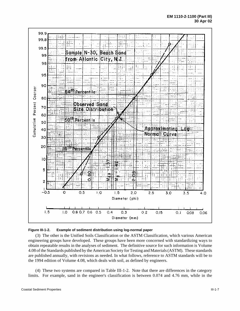
Figure III-1-2. Example of sediment distribution using log-normal paper . . . . . . . . . . . . . . . . . . . III-1-7
Figure III-1-3. Suggested composite sediment sample groups on a typical profile - examplefrom CHL Field Research Facility, Duck, NC . . . . . . . . . . . . . . . . . . . . . . . . . . . . III-1-12
Figure III-1-4. Unconfined ultimate strength of three rock types (Hardin 1966) . . . . . . . . . . . . . III-1-18
Figure III-1-5. Drag coefficient as a function of Reynolds Number (Vanoni 1975) . . . . . . . . . . . III-1-22
Figure III-1-6. Fall velocity of quartz spheres in air and water (Vanoni 1975) . . . . . . . . . . . . . . . III-1-25

EM 1110-2-1100 (Part III)30 Apr 02
Coastal Sediment Properties III-1-1
Chapter III-1Coastal Sediment Properties
III-1-1. Introduction
a. Bases of sediment classification.
(1) Several properties of sediments are important in coastal engineering. Most of these properties canbe placed into one of three groups: the size of the particles making up the sediment, the composition of thesediment, or bulk characteristics of the sediment mass.
(2) In some cases (in clay, for example) there are strong correlations among the three classificationgroups. A clay particle is, in the compositional sense, a mineral whose molecules are arranged in sheets thatfeature orderly arrays of silicon, oxygen, aluminum, and other elements (Lambe and Whitman 1969). Clayparticles are small and platey. They are small in part because they originate from the chemical modificationand disintegration of relatively small pre-existing mineral grains and because the sheet-like minerals are notstrong enough to persist in large pieces. The geologist's size classification defines a particle as clay if it isless than 0.0039 mm. Because a clay particle is so small, it has a large surface area compared to its volume.This surface area is chemically active and, especially when wet, the aggregate of clay surfaces produces thecohesive, plastic, and slippery characteristics of its bulk form. Thus, the three classifications each identifythe same material when describing “clay.”
(3) On the other hand, most grains of beach sand are quartz, a simpler and chemically more inert materialthan clay minerals. In the geologist's size classification, sand grains are at least 16 times larger and may bemore than 500 times larger in diameter than the largest clay particle (4,000 to more than 100 million timeslarger in volume). At this size, the force of gravity acting on individual sand grains dwarfs the surface forcesexerted by those sand grains, so the surface properties of sand are far less important than surface propertiesof clay particles. Because sand grains do not stick together, a handful of pure dry sand cannot be picked upin one piece like a chunk of clay. Several differences between clay and sand are summarized onTable III-1-1. More inclusive discussions of sediment sizes, compositions, and bulk properties are given laterin this chapter.
Table III-1-1Relations Among Three Classifications for Two Types of Sediment
Bases of Classification
Name of Sediment Usual Composition Size Range, Wentworth Bulk Properties
Clay Clay Minerals(sheets of silicates)
Less than 0.0039 mm CohesivePlastic under stressSlipperyImpermeable
Sand Quartz(SiO2)
Between 0.0625 mm and2.00 mm
NoncohesiveRigid under stressGrittyPermeable
b. Sediment properties important for coastal engineering. Sediment properties of material existing atthe project site, or that might be imported to the site, have important implications for the coastal engineeringproject. The following sections briefly discuss several examples of ways that sediment properties affectcoastal engineering projects and illustrate their importance.

EM 1110-2-1100 (Part III)30 Apr 02
III-1-2 Coastal Sediment Properties
(1) Properties important in dredging.
(a) A hydraulic dredge needs to entrain sediment from the bottom and pump it through a pipe. Theentrainment and the pumping are both affected by the properties of the sediment to be dredged. The subjectis briefly treated in the following paragraphs, but more details on dredging practice can be obtained frombooks by Turner (1984) and Huston (1970). Other information is available through the Dredging ResearchProgram of the U.S. Army Corps of Engineers.
(b) Sediment can be classified for entrainment by a hydraulic dredge as fluid, loose, firm, or hard. Fluidmuds and loose silt or sand can be entrained relatively easily by dragheads. Firm sand, stiff clay, andorganically bound sediment may require a cutterhead dredge to loosen the sediment. Usually, hard materialsuch as rock or coral is not suitable for hydraulic dredging unless the material has previously been wellbroken.
(c) Sediment can be classified for pumping by a hydraulic dredge as cohesive, noncohesive, or mitigated(Turner 1984). Cohesive sediments get transported through the pipe as lumps and nodules whereasnoncohesive sediments disperse as a slurry, which is more easily pumped through the pipe. Mitigatedsediments consist mainly of noncohesive sediments with a small amount of clay, which increases the transportefficiency of the pipe.
(d) The diameter of the pipe and the size of the pump limit the size of the material which can be pumped.Usually, oversize material is prevented from entering the pipeline of a suction dredge by a grid placed acrossthe draghead, or the cutterhead reduces material entering the pipeline to adequate size.
(e) Another property of the sediment important in dredging is the degree of its cohesiveness that allowsthe sediment to stand in near-vertical banks while being dredged. A dredge works more efficiently if thematerial will maintain such a steep “face” during the dredging process. Muds and loose sands that flow likeliquids lack this property.
(f) The above statements apply to those dredging systems that remove material from the bottom througha pipeline by a pump. Such hydraulic dredges are not always the most feasible dredging system to usebecause of space constraints, navigation requirements, dredging depth, sediment properties, or disposaloptions. Under some conditions, mechanical dredges, which include a grab bucket operated from a derrick,or a dipper dredge (power shovel) on a barge (Huston 1970), may be more desirable. When mechanicaldredges are used, looser sediments are usually dredged with a bucket and harder sediments with a dipper.
(2) Properties important in environmental questions.
(a) Recently, environmental problems associated with the handling and deposition of sediment havereceived increased attention. These concerns most frequently arise from dredging operations, but can occuranytime sediment is introduced into the marine environment. The usual issues involve the burial of bottom-dwelling organisms, the blockage of light to bottom-dwelling and water-column organisms, and the toxicityof the sediments.
(b) The sediment property of most environmental consequence is size. Turbidity in the water columndepends on the fall velocity of the sediment particles, which is a strong function of the grain size. Turbidwaters can be carried by currents away from the immediate project site, blocking the light to organisms overa wide area and, as the sediments settle out, blanketing the bottom at a rate faster than the organisms canaccommodate. Fine sediments (silts and clays) get greater scrutiny under environmental regulation becausethey produce greater and longer-lasting turbidity, which will impact larger areas of the seafloor than will

EM 1110-2-1100 (Part III)30 Apr 02
Coastal Sediment Properties III-1-3
coarser, sand-sized material. The dredging of sand usually encounters less severe environmental objection,provided that there are few fines mixed with it and that the site has no prior toxic chemical history.
(c) Environmental regulation is changing, and many regulatory questions are outside the usual experienceof coastal engineers. However, a basic coastal engineering contribution to facilitating the progress of aproject through regulatory review is the early collection of relevant sediment samples from the site andobtaining accurate data on their size, composition, and toxicity.
(3) Properties important in beach fills.
(a) Beach fills have two primary functions: to provide temporary protection to upland property, and toincrease temporarily the recreational space along the shore. Neither function can be well satisfied withsediment finer than sand. Because the recreational function is inhibited by material coarser than sand, andbecause fill coarser than sand is frequently less available, the primary beach fill material is usually sand.
(b) The source sediment for a beach fill is known as the borrow material, and the sediment on the beachprior to the fill is known as the native material. The sediment property most important for design is the sizedistribution of the borrow and native sands. The art of beach fill design consists of calculating the volumeof borrow with a given size distribution that will produce a required volume of beach fill.
(c) Ideally, the median size of the borrow sand should not be less than the median size of the native sand,and the spread of the sizes in the borrow size distribution should not exceed the spread of sizes in the nativesand. Often it is impossible to meet these ideal conditions because suitable borrow material does not existin adequate volume at a reasonable cost. Further, on severely eroded beaches, the native sand may be skewedto coarser size ranges because the fines have eroded out, producing unrealistic requirements for borrow sandsize distribution.
(d) Beach fill design aims to compensate for the differences between borrow sand and native sand,usually by overfilling with borrow sand and assuming preferential loss of the fine fractions. A favorablefeature of beach fill technology is the accidental, partial loss of the fine fraction during the dredging andhandling between borrow and beach. There have been cases (mostly anecdotal) where such handling losseshave produced sand fill on the beach that is coarser than the borrow sand from which the fill was derived.
(e) The shore protection and the recreational qualities of a beach fill conflict when coarser sediment sizesare used. Usually, a beach provides more protection against erosion when its particles are coarser (also whenthey are more angular and more easily compacted). However, fill material larger than sand size (about2.0 mm) will lessen the recreational value of the beach. Also odor and color of beach fill may be objectionalto recreational users; but usually, if the grain size of the material is adequate, the objectional odor and colorare temporary.
(4) Properties important in scour protection.
(a) Scour, the localized removal of bed material below its natural elevation, usually occurs near (and isusually caused by) marine structures such as jetties, seawalls, bridge pilings, etc. These types of structurescan accelerate tidal currents, focus wave energy, and increase turbulence in the water column.
(b) To prevent scour, it is usual to place a layer of less erodible material on the surface of the sedimentthat is subject to erosion. Such a layer is called a revetment or scour blanket. A typical revetment consistsof broken rock, known as riprap, which is essentially a sediment consisting of large rock particles. Thesedimentary properties of riprap which are important as scour protection include its size distribution, densityof the rock material, and the porosity and permeability of the material as placed. The riprap must be heavy
EM 1110-2-1100 (Part III)30 Apr 02
III-1-4 Coastal Sediment Properties
enough to resist movement under design currents, the porosity and thickness of the riprap must be adequateto dissipate fluid energy before it reaches the underlying material being protected, and the permeability mustbe adequate to satisfactorily relieve pressure buildup at the seafloor-revetment interface.
(c) For long-term protection, riprap must consist of dense, durable material of blocky shape. Porouscarbonate rocks such as coral and some limestones are not satisfactory, and thin slabs of material of anycomposition (such as shale) are usually more mobile than blocky shapes having the same weight. However,in any situation, economics and available materials may make it advantageous to use materials that departfrom the ideal.
(d) It should be recognized that scour protection in coastal engineering differs from scour protectionencountered in typical transportation projects both in the magnitude of the forces and in their reversingdirections. Though scour protection design for highways is a well-developed art with extensivedocumentation, the direct transferal of highway riprap experience to coastal problems is usuallyunsatisfactory.
(5) Properties important in sediment transport studies.
(a) The underlying physics of how water moves sediment is not well understood. This is, perhaps, onereason for the large number of formulas (often conflicting) which have been proposed to predict transportrates. These formulas are usually functions of fluid properties, flow condition properties, and sedimentproperties. Sediment properties commonly used include: grain size, grain density, fall velocity, angle ofrepose, and volume concentration. Sediment size distribution and grain shape are also important.
(b) One method used to study sediment transport is to follow the movement of marked (tracer) particlesin the nearshore environment. Ideally, tracers should react to coastal processes that move sediment in amanner identical to the native sand, yet provide some signal to the investigator that will distinguish the tracerfrom the native material. In the last two decades, the most common tracer has been dyed native sand grains.Typically representative samples of sand taken from the site are dyed with a fluorescent dye and thenreintroduced to their environment. Care must be taken to ensure that the dying process does not significantlyalter the sediment size or density. Transport of these tracers is then monitored by sampling. Because of theirdilute distribution, tracers are a very labor-intensive means of studying sediment movement.
(c) Native sand tracers (trace minerals, heavy minerals) have been used to interpret sediment movement,but usually these tracers have a size and density that differ from the majority of grains on the beach. Theproblem becomes more complicated as beach fills become more common, and inadvertently introducenon-native tracer grains. See Galvin (1987) for a more thorough discussion of this topic.
(d) Recently, a few sensors have become available that can measure the concentration of movingsediment. These sensors are generally quite sensitive to grain size and require calibration using sedimentsobtained onsite. See, for example, a discussion of an optical backscatter sensor (Downing, Sternberg, andLister 1981).
III-1-2. Classification of Sediment by Size
a. Particle diameter.
(1) One of the most important characteristics of sediment is the size of the particles. The range of grainsizes of practical interest to coastal engineers is enormous, covering about seven orders of magnitude, fromclay particles to large breakwater armor stone blocks. A particle's size is usually defined in terms of itsdiameter. However, since grains are irregularly shaped, the term diameter can be ambiguous. Diameter is

EM 1110-2-1100 (Part III)30 Apr 02
Coastal Sediment Properties III-1-5
normally determined by the mesh size of a sieve that will just allow the grain to pass. This is defined as aparticle’s sieve diameter. When performed in a standard manner, sieving provides repeatable results,although there is some uncertainty about how the size of a sieve opening relates to the physical size of theparticle passing through the opening. (See page 58 of Blatt, Middleton, and Murray (1980) for furtherdiscussion.)
(2) Another way to define a grain's diameter is by its fall velocity. A grain's sedimentation diameter isthe diameter of a sphere having the same density and fall velocity. This definition has the advantage ofrelating a grain's diameter to its fluid behavior, which is the usual ultimate reason for needing to determinethe diameter. However, a settling tube analysis is somewhat less reproducible than a sieve analysis, andtesting procedures have not been standardized. Other diameter definitions that have been occasionally usedinclude the nominal diameter, the diameter of a sphere having the same volume as the particle; and the axialdiameter, the length of one of the grain's principal axes, or some combination of these axes.
(3) For nearly spherical particles, as many sand grains are (but most shell and shell fragments are not),there is little difference in these definitions. When reporting the results of an analysis, it is always appropriateto define the diameter (or describe the measurement procedure), particularly if the sieve diameter is not beingused.
(4) Usually, there is a need to characterize an appropriate diameter for an aggregation of particles, ratherthan the diameter of a single particle. Even the best-sorted natural sediments have a range of grain sizes.Most sediment samples found in nature have a few relatively large particles covering a wide range ofdiameters and many small particles within a small range of diameters. That is, most natural sediment sampleshave a highly skewed distribution, in an absolute sense. However, if size classes are based upon a logarithmic(power of 2) scale and if the contents of each size fraction are considered by weight (not by the number ofparticles), then most typical sediment samples will have a distribution that is near Gaussian (or normal).When such sediment samples are plotted as a percentage of the total weight of the sample being sieved, thesediment size distribution that results usually approximates a straight line on a log-normal graph. This lineis known as the log-normal distribution. Meaningful descriptions of the distributions of this type of data canbe made using standard statistical parameters.
(5) Sediment size data normally come from the weight of sediment that accumulates on each sieve in anest of graduated sieves. This can be plotted on semilog paper as shown in Figure III-1-1 (ENG form 2087)or on log-normal paper as shown in Figure III-1-2.
b. Sediment size classifications.
(1) The division of sediment sizes into classes such as cobbles, sand, silt, etc., is arbitrary, and manyschemes have been proposed. However, two classification systems are in general use today by coastalengineers. Both have been adopted from other fields.
(2) The first is the Modified Wentworth Classification, which is generally used in geologic work.Geologists have been particularly active in sediment size research because they have long been interested ininterpreting slight differences in size as indicating particular processes or events in the geologic past. Asummary of geological work applicable to coastal engineering is found in Chapter 3 of the book by Blatt,Middleton, and Murray (2nd ed., 1980).

EM 1110-2-1100 (Part III)
30 Apr 02
III-1-6C
oastal Sediment Properties
Figure III-1-1. Example of sediment distribution using semilog paper; sample 21c - foreshore at Virginia Beach
GRAVEL SAND FINES COBBLES
CO/>RSE FINE MEDIUM FINE SILT SIZES CLAY SIZES
U.S. STi\NDARD SIEVE SIZES
3" 2" 1'' 3 / 4" 3/8" 4 10 20 40 60 100 200
100 I I I I I I
I I f-.._
~~ I I
90 I I I ~ I I
11 I I
80
f---I C) 70
w :s:
I I I \ I I
I I I \ I I I I I \ I I
I I I \ I I I I I \ I I
>- 60 m I I I I I 0::: I I I I I w 50 z [;:: I I I I I
I I I I I f--- 40 z w I I I I I u 0::: w 30
II I \ I
Q. I I I I I
20 I I I \ I I
I I I I I
10
I I I \: I II I
I I I iR I
0 II I I '"> r-e--I I I I ~
100 10 1.0 0.1 0.01 0.001
GRAIN SIZE IN MILLIMETERS
EM 1110-2-1100 (Part III)30 Apr 02
Coastal Sediment Properties III-1-7
Figure III-1-2. Example of sediment distribution using log-normal paper(3) The other is the Unified Soils Classification or the ASTM Classification, which various American
engineering groups have developed. These groups have been more concerned with standardizing ways toobtain repeatable results in the analyses of sediment. The definitive source for such information is Volume4.08 of the Standards published by the American Society for Testing and Materials (ASTM). These standardsare published annually, with revisions as needed. In what follows, reference to ASTM standards will be tothe 1994 edition of Volume 4.08, which deals with soil, as defined by engineers.
(4) These two systems are compared in Table III-1-2. Note that there are differences in the categorylimits. For example, sand in the engineer's classification is between 0.074 and 4.76 mm, while in the

EM 1110-2-1100 (Part III)31 July 03
III-1-8 Coastal Sediment Properties
Table III-1-2Sediment Particle SizesASTM (Unified) Classification1 U.S. Std. Sieve2 Size in mm Phi Size Wentworth Classification3
Boulder
Cobble
Coarse Gravel
Fine Gravel
Coarse Sand
Medium Sand
Fine Sand
Fine-grained Soil:
Clay if PI $ 4 and plot of PI vs. LL ison or above “A” line and the presenceof organic matter does not influenceLL.
Silt if PI < 4 and plot of PI vs. LL isbelow “A” line and the presence oforganic matter does not influence LL.
(PI = plasticity limit; LL = liquid limit)
12 in. (300 mm)
3 in. (75 mm)
3/4 in. (19 mm)
2.533.5
4 (4.75 mm)5678
10 (2.0 mm)1214161820253035
40 (0.425 mm)4550607080
100120140170
200 (0.075 mm)230270325400
4096.1024.256.128.107.6490.5176.1164.0053.8245.2638.0532.0026.9122.6319.0316.0013.4511.319.518.006.735.664.764.003.362.832.382.001.681.411.191.000.840.710.590.500.4200.3540.2970.2500.2100.1770.1490.1250.1050.0880.0740.06250.05260.04420.03720.03120.01560.00780.00390.001950.000980.000490.000240.000120.000061
-12.0-10.0-8.0-7.0-6.75-6.5-6.25-6.0-5.75-5.5-5.25-5.0-4.75-4.5-4.25-4.0-3.75-3.5-3.25-3.0-2.75-2.5-2.25-2.0-1.75-1.5-1.25-1.0-0.75-0.5-0.250.00.250.50.751.01.251.51.752.02.252.52.753.03.253.53.754.04.254.5
4.755.06.07.08.09.0
10.011.012.013.014.0
Boulder Large Cobble
Small Cobble
Very Large Pebble
Large Pebble
Medium Pebble
Small Pebble
Granule
Very Coarse Sand
Coarse Sand
Medium Sand
Fine Sand
Very Fine Sand
Coarse Silt
Medium Silt Fine Silt Very Fine Silt Coarse Clay
Medium Clay
Fine Clay
Colloids
1 ASTM Standard D 2487-92. This is the ASTM version of the Unified Soil Classification System. Both systems are similar (fromASTM (1994)).2 Note that British Standard, French, and German DIN mesh sizes and classifications are different.3 Wentworth sizes (in mm) cited in Krumbein and Sloss (1963).

EM 1110-2-1100 (Part III)30 Apr 02
Coastal Sediment Properties III-1-9
φ ' & log2 D (III-1-1a)
D ' 2&φ (III-1-1b)
geologist's classification, sand is between 0.0625 and 2.0 mm. In describing a sediment, it is necessary to saywhich classification system is being utilized.
c. Units of sediment size.
(1) Table III-1-2 lists three ways to specify the size of a sediment particle: U.S. Standard sieve numbers,millimeters, and phi units. A sieve number is approximately the number of square openings per inch,measured along a wire in the wire screen cloth (Tyler 1991). Available sieve sizes can be obtained fromcatalogs on construction materials testing such as Soiltest (1983). The millimeter dimension is the length ofthe inside of the square opening in the screen cloth. This square side dimension is not necessarily themaximum dimension of the particle which can get through the opening, so these millimeter sizes must beunderstood as nominal approximations to sediment size. Table III-1-2 shows that the Wentworth scale hasdivisions that are whole powers of 2 mm. For example, medium sands are those with diameters between 2-2
mm and 2-1 mm. This property of powers of 2-mm class limits led Krumbein (1936) to propose a phi unitscale based on the definition:
where D is the grain diameter in millimeters. Phi diameters are indicated by writing φ after the numericalvalue. That is, a 2.0-φ sand grain has a diameter of 0.25 mm. To convert from phi units to millimeters, theinverse equation is used:
(2) The benefits of the phi unit include: (a) it has whole numbers at the limits of sediment classes in theWentworth scale; and (b) it allows comparison of different size distributions because it is dimensionless.Disadvantages of this phi unit are: (a) the unit gets larger as the sediment size gets smaller, which is bothcounterintuitive and ambiguous; (b) it is difficult to physically interpret size in phi units without considerableexperience; and (c) because it is a dimensionless unit, it cannot represent a unit of length in physicalexpressions such as fall velocity or Reynolds number.
d. Median and mean grain sizes.
(1) All natural sediment samples contain grains having a range of sizes. However, it is frequentlynecessary to characterize the sample using a single typical grain diameter as a measure of the central tendencyof the distribution. The median grain diameter Md is the sample characteristic most often chosen. Thedefinition of Md is that, by weight, half the particles in the sample will have a larger diameter and half willhave a smaller. This quantity is easily obtained graphically, if the sample is sorted by sieving or othermethod, and the weight of the size fractions are plotted, as seen in Figures III-1-1 and III-1-2.
(2) The median diameter is also written as D50. Other size fractions are similarly indicated. For example,D90 is the diameter for which 90 percent of the sediment, by weight, has a smaller diameter. An equivalentdefinition holds for the median of the phi-size distribution φ50 or for any other size fraction in the phi scale.
(3) Another measure of the central tendency of a sediment sample is the mean grain size. Severalformulas have been proposed to compute this quantity, given a cumulative size distribution plot of the sample(Otto 1939, Inman 1952, Folk and Ward 1957, McCammon 1962). These formulas are averages of 2, 3, 5,or more symmetrically selected percentiles of the phi frequency distribution. Following Folk (1974):

EM 1110-2-1100 (Part III)30 Apr 02
III-1-10 Coastal Sediment Properties
Mφ '(φ16 % φ50 % φ84 )
3(III-1-2)
σφ '(φ84 & φ16)
4%
(φ95 & φ5)6
(III-1-3)
αφ 'φ16 % φ84 & 2(φ50 )
2(φ84 & φ16 )%
φ5 % φ95 & 2(φ50)2(φ95 & φ5)
(III-1-4)
βφ 'φ95 & φ5
2.44 (φ75 & φ25)(III-1-5)
where Mφ is the estimated mean grain size of the sample in phi units. This can be converted to a lineardiameter using Equation 1-1b. The median and mean grain sizes are usually quite similar for most beachsediments. For example, a study of 465 sand samples from three New Jersey beaches, the mean averagedonly 0.01 mm smaller than the median for sands having an average median diameter of 0.30 mm (1.74 phi)(Ramsey and Galvin 1977). If the grain sizes in a sample are log-normally distributed, the two measures areidentical. Since the median is easier to determine and the mean does not have a universally accepteddefinition, the median is normally used in coastal engineering to characterize the central tendency of asediment sample.
e. Higher order moments.
(1) Additional statistics of the sediment distribution can be used to describe how the sample varies froma log-normal distribution. The standard deviation is a measure of the degree to which the sample spreads outaround the mean (i.e., its sorting). Following Folk (1974), the standard deviation can be approximated by:
where σφ is the estimated standard deviation of the sample in phi units. For a completely uniform sedimentφ05, φ16, φ84, and φ95 are all the same, and thus, the standard deviation is zero. There are also qualitativedescriptions of the standard deviation. A sediment is described as well-sorted if all particles have sizes thatare close to the typical size (small standard deviation). If the particle sizes are distributed evenly over a widerange of sizes, then the sample is said to be well-graded. A well-graded sample is poorly sorted; a well-sorted sample is poorly graded.
(2) The degree by which the distribution departs from symmetry is measured by the phi coefficient ofskewness αφ defined in Folk (1974) as:
(3) For a perfectly symmetric distribution, the skewness is zero. A positive skewness indicates there isa tailing out toward the fine sediments, and conversely, a negative value indicates more outliers in the coarsersediments.
(4) The phi coefficient of kurtosis βφ is a measure of the peakedness of the distribution; that is, theproportion of the sediment in the middle of the distribution relative to the amount in both tails. FollowingFolk (1974), it is defined as:
Values for the mean and median grain sizes are frequently converted from phi units to linear measures.However, the standard deviation, skewness, and kurtosis should remain in phi units because they have nocorresponding dimensional equivalents. If these terms are used in equations, they are used in theirdimensionless phi form. Relative relationships are given for ranges of standard deviation, skewness, andkurtosis in Table III-1-3.

EM 1110-2-1100 (Part III)30 Apr 02
Coastal Sediment Properties III-1-11
Table III-1-3Qualitative Sediment Distribution Ranges for Standard Deviation, Skewness,and Kurtosis
Standard Deviation
Phi Range Description
<0.35 Very well sorted
0.35-0.50 Well sorted
0.50-0.71 Moderately well sorted
0.71-1.00 Moderately sorted
1.00-2.00 Poorly sorted
2.00-4.00 Very poorly sorted
>4.00 Extremely poorly sorted
Coefficient of Skewness
<-0.3 Very coarse-skewed
- 0.3 to - 0.1 Coarse-skewed
- 0.1 to +0.1 Near-symmetrical
+0.1 to +0.3 Fine-skewed
>+0.3 Very fine-skewed
Coefficient of Kurtosis
<0.65 Very platykurtic (flat)
0.65-0.90 Platykurtic
0.90-1.11 Mesokurtic (normal peakedness)
1.11-1.50 Leptokurtic (peaked)
1.50-3.00 Very leptokurtic
>3.00 Extremely leptokurtic
f. Uses of distributions. The median grain size is the most commonly used sediment size characteristic,and it has wide application in coastal engineering practice. The standard deviation of sediment samples hasbeen used in several ways, including beach-fill design (see Hobson (1977), Ch. 5, Sec. III,3) and sedimentpermeability (Krumbein and Monk 1942). When a set of samples are taken from a single project site, theywill frequently show little or no consistent variation in median diameter. In this case, various higher ordermoments are usually used to distinguish different depositional environments. There is an extensive literatureon the potential application of the measures of size distribution; see, for example, Inman (1957), Folk andWard (1957), McCammon (1962), Folk (1965, 1966), Griffiths (1967), and Stauble and Hoel (1986).
g. Sediment sampling procedures.
(1) Although a beach can only be composed of the available sediments, grain size distributions changein time and space. In winter, beach distributions are typically coarser and more poorly sorted than in summer.Also, typically, there is more variability in the foreshore and the bar/trough regions than in the dunes and thenearshore.
(2) While a single sample is occasionally sufficient to grossly characterize the sediments at a site, usuallya set of samples is obtained. Combining samples from across the beach can reduce the high variability inspacial grain size distributions on beaches (Hobson 1977). Composite samples are created by eitherphysically combining several samples before sieving or by mathematically combining the individual sample

EM 1110-2-1100 (Part III)30 Apr 02
III-1-12 Coastal Sediment Properties
Figure III-1-3. Suggested composite sediment sample groups on a typical profile - example fromField Research Facility, Duck, NC
weights. The set of samples obtained can be fairly small if the intent is only to characterize the beach as awhole. However, if the intent is to compare and contrast different portions of the same beach, many moresamples are needed. In this case it is usually necessary to develop a sampling scheme prior to fieldwork.
(3) In the cross-shore it is recommended that samples be collected at all major changes in morphologyalong the profile, such as dune base, mid-berm, mean high water, mid-tide, mean low water, trough, bar crest,and then at 3-m intervals to the depth of closure (Stauble and Hoel 1986). In the longshore direction,sediment sampling should coincide with survey profile lines so that the samples can be spatially located andrelated to morphology and hydrodynamic zones. Shoreline variability and engineering structures should beconsidered in choosing sampling locations. A suggested rule of thumb is that a sampling line be spaced everyhalf mile, but engineering judgment is required to define adequate project coverage.
(4) Samples collected along profile sub-environments can be combined into composite groups of similardepositional energy levels as seen in Figure III-1-3. Intertidal and subaerial beach samples have been foundto be the most usable composites to characterize the beach and nearshore environment. Stauble and Hoel(1986) found that a composite containing the mean high water, mid-tide, and mean low water gave the bestrepresentation of the foreshore beach.

EM 1110-2-1100 (Part III)30 Apr 02
Coastal Sediment Properties III-1-13
EXAMPLE PROBLEM III-1-1
FIND:The statistics of the sediment size distribution shown in Figure III-1-2 and their qualitative
descriptions.
GIVEN:The needed phi values are: φ05 = 0.56, φ16 = 0.80, φ25 = 0.93, φ50 = 1.37, φ75 = 1.87, φ84 = 2.08,
and φ95 = 2.48.
SOLUTION:In phi units, the median grain size is given as:
φ50 = Mdφ = 1.37φ
From Equation 1-1b, the median grain size in millimeters is found as:
Md = 2-1.37 = 0.39 mm
From Equation 1-2, the mean grain size is found in phi units as:
Mφ = (0.80 + 1.37 + 2.08) / 3 = 1.42φ
From Equation 1-1b, this is converted to millimeters as:
D = 2-1.42 = 0.37 mm
From Equation 1-3, the standard deviation is found as:
σφ = (2.08 - 0.80)/4 + (2.48 -0.56)/6.0 = 0.32 + 0.32 = 0.64 φ
From Equation 1-4, the coefficient of skewness is found as:
αφ = 0.055 + 0.078 = 0.13
From Equation 1-5, the coefficient of kurtosis is found as:
βφ = 1.92 / 2.29 = 0.84
Thus, using Tables III-1-2 and III-1-3, the sediment is a medium sand (Wentworth classification),it is moderately well sorted, and the distribution is fine-skewed and platykurtic.

EM 1110-2-1100 (Part III)30 Apr 02
III-1-14 Coastal Sediment Properties
h. Laboratory procedures.
(1) Several techniques are available to analyze the size of beach materials, and each technique isrestricted to a range of sediment sizes. Pebbles and coarser material are usually directly measured withcalipers. However, this is not practical for sediments smaller than about 8 mm. Coarse sieves can also beused for material up to about 75 mm.
(2) Sand-sized particles (medium gravels through coarse silt) are usually analyzed using sieves. Thisrequires an ordered stack of sieves of square-mesh woven-wire cloth. Each sieve in the stack differs fromthe adjacent sieves by having a nominal opening less than the opening of the sieve above it and greater thanthe opening of the sieve below it. A pan is placed below the bottom sieve. The sample is poured into the topsieve, a lid is placed on top, and the stack is placed on a shaker, usually for about 15 min. The differentgrains fall through the stack of sieves until each reaches a sieve that is too fine for it to pass. Then the amountof sediment in each sieve is weighed. ASTM Standard D422-63 (Reapproved 1990) is the basic standard forparticle size analysis of soils, including sieving sedimentary materials of interest to coastal engineers. Theapplication of D422 requires sample preparation described in Standard D421-85 (Reapproved 1993). Thewire cloth sieves should meet ASTM Specification E-11.
(3) Sieves are graduated in size of opening according to the U.S. standard series or according to phi sizes.U.S. standard sieve sizes are listed in Table III-1-2, and the most commonly used sieves are shown inFigure III-1-1. Phi sized sieve openings vary by a factor of 1.19 from one sieve size to the next (by the fourthroot of 2, or 0.25 phi units); e.g., 0.25, 0.30, 0.35, 0.42, and 0.50 mm.
(4) The range of sieve openings must span the range of sediment sizes to be sieved. Typically, about 6full-height sieves or 13 half-height sieves plus a bottom pan are used in the analysis of a particular sediment.If 6 sieves are used, each usually varies in size from its adjacent neighbors by a half phi; if 13 sieves are used,each usually varies by a quarter phi. Normally, about 40 grams of sediment is sieved. More is needed if thereare large size fractions (see ASTM Standard D2487-94).
(5) Determination of sediment size fractions for silts and clays is usually not necessary. Rather it isnormally noted that a certain percentage of the material are fines with diameters smaller than the smallestsieve. When measurements are needed, the pipette method or the hygrometer method is usually used. Bothof these methods are based upon determining the amount of time that different size fractions remain insuspension. These are discussed in Vanoni (1975). Coulter counters have also been used occasionally.
III-1-3. Compositional Properties
a. Minerals.
(1) Because of its resistance to physical and chemical changes and its common occurrence in terrestrialrocks, quartz is the mineral most commonly found in littoral materials. On temperate latitude beaches, quartzand feldspar grains commonly account for more than 90 percent of the material (Krumbein and Sloss 1963,p.134), and quartz, on average, accounts for about 70 percent of beach sand. However, it is important torealize that on individual beaches the percentage of quartz grains (or any other mineral) can range fromessentially zero to 100 percent. Though feldspars are more common on the surface of the earth as a whole,comprising approximately 50 percent of all crustal rocks to quartz's approximately 12 percent (Ritter 1986),feldspars are more subject to chemical weathering, which converts them to clay minerals, quartz, andsolutions. Since quartz is so inert, it accumulates during weathering processes. Thus, feldspars and relatedsilicates are more commonly encountered in coastal sediment close to sources of igneous and metamorphicrocks, especially mountainous and glaciated coasts where streams and ice carry unweathered sediment

EM 1110-2-1100 (Part III)30 Apr 02
Coastal Sediment Properties III-1-15
immediately to the shore. Quartz sand and clay are more common on shores far from mountains whereweathering has had more time to reduce the relative proportions of feldspars and related silicates.
(2) Most carbonate sands owe their formation to organisms (both animal and vegetable) that precipitatecalcium carbonate by modifying the very local chemical environment of the organism to favor carbonatedeposition. Calcium carbonate may be deposited as calcite or aragonite, but aragonite is unstable and changeswith time to either calcite or solutions. Calcite or limestone, the rock made from calcite, may, under someconditions, be altered to dolomite by the partial replacement of the calcium with magnesium. Carbonatesands can contribute up to 100 percent of the beach material, particularly in situations where it is producedin the local marine environment and there are limited terrestrial sediment supplies, such as reef-fringed,tropical island beaches. These sands are generally composed of a combination of shell and shell fragments,oolites, coral fragments, and algal fragments (Halimeda, foraminiferans, etc.). When carbonate shell is mixedwith quartz sand, it may be necessary to dissolve out the shell to get a meaningful representation of each sizefraction. ASTM Standard 4373 describes how to determine the calcium carbonate content of a beach.
(3) Other minerals that frequently form a small percentage of beach sands are normally referred to asheavy minerals, because their specific gravities are usually greater than 2.87. These minerals are frequentlyblack or reddish and may, in sufficient concentrations, color the entire beach. The most common of theseminerals (from Pettijohn (1957)) are andalusite, apatite, augite, biotite, chlorite, diopside, epidote, garnet,hornblende, hypersthene-enstatite, ilmenite, kyanite, leucoxene, magnetite, muscovite, rutile, sphene,staurolite, tourmaline, zircon, and zoisite. Their relative abundance is a function of their distribution in thesource rocks of the littoral sediments and the weathering process. Heavy minerals have been occasionallyused as natural tracers to identify sediment pathways from the parent rocks (Trask 1952; McMaster 1954;Giles and Pilkey 1965; Judge 1970).
In coastal engineering work, knowledge of the sediment composition is not normally important in its ownright, but it is closely related to other important parameters such as sediment density and fall velocity.
b. Density.
(1) Density is the mass per unit volume of a material, which, in SI units, is measured in kilograms percubic meter (kg/m3). Sediment density is a function of its composition. Minerals commonly encounteredin coastal engineering include quartz, feldspar, clay minerals, and carbonates. Densities for these mineralsare given in Table III-1-4.
(2) Quartz is composed of the mineral silicon dioxide. Feldspar refers to a closely related group of metalaluminium silicate minerals. The most common clay minerals are illinite, montmorillonite, and kaolinite.Common carbonate minerals include calcite, aragonite, and dolomite. However, carbonate sands are usuallynot simple, dense solids; but rather the complex products of organisms which produce gaps, pores, and holeswithin the structure, all of which tend to lower the effective density of carbonate sand grains. Thus, carbonatesands frequently have densities less than quartz.
(3) The density of a sediment sample may be calculated by adding a known weight of dry sediment toa known volume of water. The change in volume is measured; this is the volume of the sediment. The sedi-ment mass (= weight / acceleration of gravity) divided by its volume is the density. A complicating factoris that small pockets of air will stay in the pores and cling to the surfaces of almost all sediments. To obtainan accurate volume reading, this air must be removed by drawing a strong vacuum over the sand-water mix-ture. ASTM Volume 4.08 gives standards for measuring the density of soils and rocks, respectively (ASTM1994).
EM 1110-2-1100 (Part III)30 Apr 02
III-1-16 Coastal Sediment Properties
Table III-1-4Densities of Common Coastal Sediments
Mineral Density kg/m3
Quartz 2,648
Feldspar 2,560 - 2,650
Illite 2,660
Montmorillonite 2,608
Kaolinite 2,594
Calcite 2,716
Aragonite 2,931
Dolomite 2,866
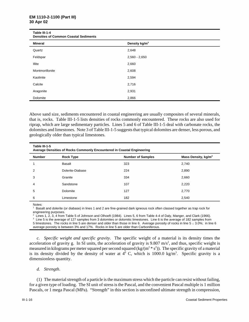
Above sand size, sediments encountered in coastal engineering are usually composites of several minerals,that is, rocks. Table III-1-5 lists densities of rocks commonly encountered. These rocks are also used forriprap, which are large sedimentary particles. Lines 5 and 6 of Table III-1-5 deal with carbonate rocks, thedolomites and limestones. Note 3 of Table III-1-5 suggests that typical dolomites are denser, less porous, andgeologically older than typical limestones.
Table III-1-5Average Densities of Rocks Commonly Encountered in Coastal Engineering
Number Rock Type Number of Samples Mass Density, kg/m3
1 Basalt 323 2,740
2 Dolerite-Diabase 224 2,890
3 Granite 334 2,660
4 Sandstone 107 2,220
5 Dolomite 127 2,770
6 Limestone 182 2,540
Notes:1 Basalt and dolerite (or diabase) in lines 1 and 2 are fine-grained dark igneous rock often classed together as trap rock forengineering purposes.2 Lines 1, 2, 3, 4 from Table 5 of Johnson and Olhoeft (1984). Lines 5, 6 from Table 4-4 of Daly, Manger, and Clark (1966).3 Line 5 is the average of 127 samples from 3 dolomites or dolomitic limestones. Line 6 is the average of 182 samples from5 limestones. The rocks in line 5 are denser and older than those in line 6. Average porosity of rocks in line 5 # 3.0%; in line 6average porosity is between 3% and 17%. Rocks in line 5 are older than Carboniferous.
c. Specific weight and specific gravity. The specific weight of a material is its density times theacceleration of gravity g. In SI units, the acceleration of gravity is 9.807 m/s2, and thus, specific weight ismeasured in kilograms per meter squared per second squared (kg/(m2 * s2)). The specific gravity of a materialis its density divided by the density of water at 40 C, which is 1000.0 kg/m3. Specific gravity is adimensionless quantity.
d. Strength.
(1) The material strength of a particle is the maximum stress which the particle can resist without failing,for a given type of loading. The SI unit of stress is the Pascal, and the convenient Pascal multiple is 1 millionPascals, or 1 mega Pascal (MPa). “Strength” in this section is unconfined ultimate strength in compression,
EM 1110-2-1100 (Part III)30 Apr 02
Coastal Sediment Properties III-1-17
which is equivalent to crushing strength. Tensile strength, which is significantly less than compressivestrength, is not discussed here, but tensile strength is usually proportional to compressive strength.
(2) The most commonly encountered material in coastal engineering is the quartz sand grain, which isvery strong indeed. A single crystal of quartz has a strength on the order of 2,500 MPa. However, asandstone, which is a composite of many sand grains, is surprisingly weak (top histogram on Figure III-1-4),being typically less than 100 MPa, or less than 4 percent of the strength of the single crystal. For this reason,sandstone is rarely used in coastal engineering construction.
(3) The difference in strength between quartz crystal and composite sandstone is due to weakintergranular cement and to flaws such as grain boundaries, bedding planes, cleavage, and joints that havea higher probability of being present in larger pieces. The data on Figure III-1-4 are excerpted from theextensive tabulation of Handin (1966), using all samples which were tested at room temperature and zeroconfining pressure.
(4) For calcium carbonate, strength varies with size in a direction opposite to that of quartz. Singlecrystals of calcite are weak (~14 MPa, depending on orientation) compared to single crystals of quartz(~2,500 MPa). But limestone rocks, made from interlocking calcium carbonate crystals, are much strongerthan single crystals of calcium carbonate, and even somewhat stronger than sandstones, as shown bycomparing the top two histograms on Figure III-1-4.
(5) The weaker rocks on the left end of the histograms of Figure III-1-4 are those with macroscopic flawssuch as bedding planes, rather than flaws in single grains. The high-strength outliers on the right end of thesandstone and limestone histograms of Figure III-1-4 are special cases. The sandstone outlier is a quartzite,a metamorphosed sandstone recrystallized with silica cement. The limestone outlier is Solnhofen limestone,which is a dense, fine-grained, uniform limestone.
(6) Dolomite is a carbonate rock allied to limestone in which about half of the calcium of calcite has beenreplaced by magnesium (both the mineral and the rock are called dolomite). On average, dolomite anddolomitic limestones make better riprap than limestone and sandstone, as suggested by comparison of thehistograms on Figure III-1-4.
(7) Where available, rocks classified commercially as trap rock (dense basalt, diorite, and related rocks)or granite (including rhyolite and dense gneiss) make even better riprap, with strength typically on the orderof 140 to 200 MPa under conditions comparable to those in Figure III-1-4.
(8) A typical specification for rock used as riprap in coastal engineering, extracted from “Low Cost ShoreProtection,” Report on Section 54, U.S. Army Corps of Engineers (1981, p. 785), is as follows:
The stone shall be free of cracks, seams, and other defects that would tend to increase unduly itsdeterioration from natural causes or breakage in handling or dumping. The stone shall weigh, whendry, not less than 150 pounds per cubic foot.* The inclusion of objectionable quantities of sand, dirt,clay, and rock fines will not be permitted. Selected granite and quartzite, rhyolite, traprock andcertain dolomitic limestones generally meet the requirements of these specifications.
*150 PCF is equivalent to 2,400 kg/m3.

EM 1110-2-1100 (Part III)30 Apr 02
III-1-18 Coastal Sediment Properties
Figure III-1-4. Unconfined ultimate strength of three rock types (after Handin(1966))
10
Sandstone N=11
Quartz s ing le crystal strength: 2,500 MPa
5
Quartz
/ 0
10 Limestone N=21
(f) Ca lc ite single cryst a l +-' strength: ~ 1 4 MPa (f) (j)
f-
4-0 5 '--(j)
_Q
E :::J Solen hofen Is. z
I 0
10 Dolomite N=8
5
0 80 160 240 320 400
Ultimate Strength , MegaPascals

EM 1110-2-1100 (Part III)30 Apr 02
Coastal Sediment Properties III-1-19
EXAMPLE PROBLEM III-1-2
FIND:The density, specific weight, and specific gravity of a sediment sample.
GIVEN:18.1 grams of the sample of dry beach sand exactly fills a small container having a volume of
10.0 cm3 after the filled container is strongly vibrated. When this amount of sand is poured into50.0 ml of water which is subjected to a strong vacuum, the volume of the sand-water mixture is56.8 ml.
SOLUTION:It is important to recognize the difference in the volume of the grains themselves, which is
6.8 cm3 (= 56.8 - 50) (a milliliter is a cubic centimeter), and the volume of the aggregate (the grainsplus the void spaces), which is 10 cm3.
Density is the sediment mass divided by its volume:
ρs = 18.1 gm / 6.8 cm3 = 2.66 gm/cm3 = 2,660 kg/m3
If this problem were in English units rather than metric, the sediment weight (in pounds force) wouldprobably be given, rather than the mass. To obtain the mass, the weight would need to be divided bythe acceleration of gravity (32.2 ft/sec2) (mass = weight / g). After dividing by the volume (in ft3), thedensity would be obtained in slugs/ft3.
The specific weight of the sand grains themselves is the density times the acceleration of gravity:
Sp wt of the grains = 2.66 gm/cm3 * 980 cm/sec2 = 2,610 gm/(cm2 * sec2) = 26,100 kg/(m2 * sec2)
The specific gravity of a material has the same value as its density when measured in gm/cm3, becausethe density of water at 40 C is 1.00 gm/cm3:
Specific Gravity = 2.66
e. Grain shape and abrasion.
(1) Grain shape is primarily a function of grain composition, grain size, original shape, and weatheringhistory. The shape of littoral material ranges from nearly spherical (e.g. quartz grains) to nearly disklike (e.g.shell fragments, mica flakes) to concave arcs (e.g. shells). Much of the early work on classifying sedimentparticle shape divided the problem into three size scales; the sphericity or overall shape of a particle, theroundness or the amount of abrasion of the corners, and the microtexture or the very fine scale roughness.These differences can be illustrated by noting that a dodecahedron has high sphericity but low roundness,while a thin oval has low sphericity but high roundness. A tennis ball has greater micro-texture than abaseball. More recent approaches to the quantification of grain shape have avoided the artificial division ofshape into sphericity, roundness, and microtexture by characterizing all the wavelengths of the grain's

EM 1110-2-1100 (Part III)30 Apr 02
III-1-20 Coastal Sediment Properties
irregularities in one procedure using fractal geometry types of analysis. See Ehrlich and Weinberg (1970),and Frisch, Evans, Hudson, and Boon (1987).
(2) Grain shape is important to coastal engineers because it affects several other properties, particularlywhen the grains are far from spherical, which is the usual assumption. These include fall velocity, sieveanalysis, initiation of motion, and also certain bulk properties, such as porosity and angle of repose. Oneparticular area of interest to coastal engineers is in the design of man-made interlocking armor units onbreakwaters that have high stability, even when stacked at a high angle of repose. Grain shape has also beenused to indicate residence time in the littoral environment. See Krinsley and Doornkamp (1973) and Margolis(1969).
(3) However, most littoral grain shapes are close enough to spheres that a detailed study of their shapeis not warranted. Frequently, a qualitative description of roundness is sufficient. This can be done bycomparing the grains in a sample to photographs of standardized grains (see Krumbein 1941; Powers 1953;Shepard and Young 1961).
(4) Among the earliest research studies in coastal engineering were investigations of sand grain abrasion,done because of the worry that abrasion of beach sand contributes to beach erosion. These investigationsfound that abrasion of the typical quartz beach sand is rarely significant. In general, recent information lendsfurther support to the conclusion of Mason (1942) that
On sandy beaches the loss of material ascribable to abrasion occurs at rates so low as to be of nopractical importance in shore protection problems.
(5) To achieve the high stress required for quartz to abrade (to fail locally), very large impact forces areneeded. These forces are developed by sudden changes in momentum, the product of mass and velocity.Given the small mass of a sand grain, large forces can be achieved only by grains moving at high velocities.But the drag on a sand grain moving in water increases as the square of its velocity, which limits sand grainvelocity to a low multiple of its fall velocity. Because fall velocities are only a few centimeters per second,it is extremely difficult to achieve a stress between impacting grains that is anywhere near the strength ofquartz. Thus, the rounding of the corners of angular quartz grains in riverine or littoral environments is a verylengthy process. Sands, silts, and clays found in the coastal environment can generally be considered as someof the stable end results of the weathering process of rocks so long as they remain on or near the surface ofthe earth.
(6) However, abrasion is common in large particles such as boulders and riprap subject to wave action.The mass of a particle increases with the cube of its diameter, so a minimum-size boulder (300 mm onTable III-1-2) compared to a minimum-size coarse sand grain (2 mm) (ASTM classification) will have(300/2)3 = 3.375 million times more mass. If that boulder was a perfect sphere in shape, and this rock sphererested with a point contact on the plane surface of another rock, then merely the weight of the boulder wouldcrush the point contact of the sphere until the area of contact increased enough to reduce the pressure of thecontact to below the crushing strength of the boulder (say 120 MPa, based on Figure III-1-4). The materialcrushed at this contact is abraded from the boulder. This process of stress concentration at points of contactis considered quantitatively by Galvin and Alexander (1981). If the boulder moves, say, with the rockingmotion imparted by the arrival of a wave crest, the slight velocity of the boulder mass provides a momentumwhich can produce impact forces in excess of crushing strength at points of contact between a boulder andits neighbors, thus abrading the rock.
(7) Because it is probable that a large rock will break along surfaces of weakness, the resulting piecesafter breakage will usually be stronger than the rock from which the pieces are broken. Thus, abraded gravel

EM 1110-2-1100 (Part III)30 Apr 02
Coastal Sediment Properties III-1-21
CDπ D 2
4ρ W 2
f
2'
π D 3
6(ρs & ρ) g (III-1-6)
Wf '43
gDCD
ρs
ρ& 1
12 (III-1-7)
pieces on a wave-washed shingle beach are apt to have greater strength than the bulk strength of the rock fromwhich the gravel was derived.
III-1-4. Fall Velocity
When a particle falls through water (or air), it accelerates until it reaches its fall or settling velocity. This isthe terminal velocity that a particle reaches when the (retarding) drag force on the particle just equals the(downward) gravitational force. This quantity figures prominently in many coastal engineering problems.While simple in concept, its precise calculation is usually not. A particle's fall velocity is a function of itssize, shape, and density; as well as the fluid density, and viscosity, and several other parameters.
a. General equation.
(1) For a single sphere falling in an infinite still fluid, the balance between the drag force and thegravitational force is:
or, solving for the velocity:
where
Wf = fall velocity
CD = dimensionless drag coefficient
D = grain diameter
ρ = density of water
ρs = density of the sediment
(2) The units of the fall velocity will be the same as the units of (gD)½. The problem now usuallybecomes one of determining the appropriate drag coefficient. Figure III-1-5, which is based upon extensivelaboratory data of Rouse and many others, shows how the drag coefficient CD varies as a function of theReynolds number (Re = Wf D/ν, where ν is the kinematic viscosity) for spherical particles. Re isdimensionless, but Wf , D, and ν must have common units of length and time.
(3) The plot in Figure III-1-5 can be divided into three regions. In the first region, Re is less than about0.5, and the drag coefficient decreases linearly with Reynolds number. This is the region of small, lightgrains gently falling at slow velocities. The drag on the grain is dominated by viscous forces, rather thaninertia forces, and the fluid flow past the particle is entirely laminar. The intermediate range is from about

EM 1110-2-1100 (Part III)
31 July 03
III-1-22C
oastal Sediment Properties
Figure III-1-5. Drag coefficient as a function of Reynolds Number (Vanoni 1975)
(_)~
_,_, c <I)
.~ .,__ .,__ <I) 0 (j
a> 0 ......
0
1 o4
103
1 o2
10
1
10- 1 10-3
' '\. r• ~
\.
--- i'llo )
'\ D,
01
10-2 10- 1
I I I I I I I I I I I I I I I I I I I I I I I I I I I I I I I I I
$ Al len; pa raffi n spheres in anil ine
t::. Allen ; air bu bbles i n water
X Al len; amber and steel spheres in water
• Amold; r ose m etal s pheres in r ape oil
0 Liebster; steel spheres in water
" Sc hmiedel; gold , si lver and lead discs in water
+ Lunnon ; st eel , br onze and lead s pheres in wate r
+ Simmons and Dewey; discs in wind- t unnel 0 Wieselber ger; s pher es in wind - t unnel
~ Wieselber ger; discs in wind - tun nel '<.
102 103 10 4 105 10 6 107 108 1 09 10 10
" ~, ~~ - I 1i I I 1i I I 111" I -. ~ - I I I-I ( I 1 1 -11 1 1 11 I I I
·' ~ .... \ va lu~ 16f 7T t ~I !z I'<
I' "" ' \ \ 8 , D e \
"~ ~~ I' \ ' \ \ r-, \ \
'\. v. ~ '~~ "'"" ~ ~ \ ~
\ Disc s ~ ~ ..... ~ .. ~ ~ - r--' --1-
' v ~ / ' 't" G \ \
Sta kes / 1'-- \ \ ~ \ \ p u \ ~~ - ' I> \ \Sphe res
\.
I II ~
10 1 o2 1 o3 104 1 o5 1 o6
Rey no lds number, Re

EM 1110-2-1100 (Part III)30 Apr 02
Coastal Sediment Properties III-1-23
C D '24Re
'24 νWf D (III-1-8)
Wf 'g D 2
18 νρs
ρ& 1 (III-1-9)
Wf ' 1.6 g Dρs
ρ& 1
12 (III-1-10)
W f ' 2.6 g Dρs
ρ& 1
12 (III-1-11)
Re > 400 to Re < 200,000. Here the drag coefficient has the approximately constant value of 0.4 to 0.6. Inthis range the particles are larger and denser, and the fall velocity is faster. The physical reason for thischange in the behavior of CD is that inertial drag forces have become predominant over the viscous forces,and the wake behind the particle has become turbulent. At about Re = 200,000 the drag coefficient decreasesabruptly. This is the region of very large particles at high fall velocities. Here, not only is the wake turbulent,but the flow in the boundary layer around the particle is turbulent as well.
(4) In the first region, Stokes found the analytical solution for CD as:
(5) This line is labeled “Stokes” in Figure III-1-5. Substituting Equation 1-8 into Equation 1-7 gives thefall velocity in this region:
(6) Note that in this region the velocity increases as the square of the grain diameter, and is dependentupon the kinematic viscosity.
(7) For the region of 400 < Re < 200,000, the approximation CD~0.5 is used in Equation 1-7 to obtain:
(8) Here it is seen that the fall velocity varies as the square root of the grain diameter and is independentof the kinematic viscosity.
(9) Similarly, in the region Re > 200,000, the approximation CD~0.2 is used in Equation 1-7 to obtain:
(10) There is a large transition region between the first two regimes (between 0.5 < Re < 400). Forquartz spheres falling in water, these Reynolds numbers correspond to grain sizes between about 0.08 mmand 1.9 mm. Unfortunately, this closely corresponds to all sand particles, as seen in Table III-1-2. Thus, forvery small particles (silts and clays), the fall velocity is proportional to D2 and can be calculated fromEquation 1-9. For gravel size particles the fall velocity is proportional to D½ and can be calculated fromEquation 1-10. However, for sand, the size of most interest to coastal engineers, no simple formula isavailable. The fall velocity is in a transition region between a D2 dependence and a D½ dependence. In thissize range, it is easiest to obtain a fall velocity value from plots such as Figure III-1-6, which show the fallvelocity as a function of grain diameter and water temperature for quartz spheres falling in both water andair. The vertical and horizontal axes are grain diameter and fall velocity, in millimeters and centimeters persecond, respectively. The short straight lines crossing the curves obliquely are various values of Re.

EM 1110-2-1100 (Part III)30 Apr 02
III-1-24 Coastal Sediment Properties
π8
CD Re 2 '
π D 3 ρs
ρ& 1 g
6 ν2
(III-1-12)
(11) The transition between the second and third regime corresponds to approximately 90-mm quartzspheres (cobbles, as shown on Table III-1-2) falling in water.
(12) Generally for grain sizes outside the range shown in Figure III-1-6 or for spheres with a densityother than quartz, or fluids other than air or water, Equation 1-7 can be used with a value of CD obtained fromFigure III-1-5. However, this is an iterative procedure involving repeated calculations of fall velocity andReynolds number. Instead, Equation 1-7 can be rearranged to yield:
This quantity, π/8 CD Re2 , can be used in Figure III-1-5 to obtain a value of CD or Re , either of which canthen be used to calculate the fall velocity.
b. Effect of density. Equation 1-7 shows that fall velocity depends on ((ρs /ρ)-1)½. For quartz sandgrains in fresh water, this factor is about 1.28. For quartz grains in ocean water, this factor reduces to about1.25 because of the slight increase in density of salt water. For quartz grains in very turbid (muddy) water,the factor will decrease somewhat more. If the suspended mud is present in a concentration of 10 percent bymass, ((ρs /ρ)-1)½ becomes 1.19. Thus, natural increases in water density encountered in coastal engineeringwill decrease the fall velocity of quartz by not much more than (1.28 - 1.19) / 1.28 = 0.07, or on the order of7 percent.
c. Effect of temperature. Temperature has an effect on the density of water; however, this is very smallcompared to its effect on the coefficient of viscosity. Changes in the fluid viscosity affect the fall velocityfor small particles but not for large. (Equation 1-8 contains a viscosity term while Equations 1-9 and 1-10do not.) Figure III-1-6 has separate lines labeled with temperatures of 0E, 10E, 20E, 30E, and 40 EC, and theselines are reversed for the two fluids. A grain will fall faster in warmer water, but slower in warmer air,compared to its fall velocities at lower temperatures. This difference is the direct result of how viscosityvaries with temperature in the two fluids.
d. Effect of particle shape.
(1) Grain shape affects the fall velocity of large particles (those larger than Re about 10 or D about 0.125mm in water) but has a negligible effect on small particles. For large grains of a given nominal diameter, theless spherical the particle, the slower the fall velocity. In Figure III-1-5 it is seen that at large Reynoldsnumbers, discs have higher CD values, and thus lower fall velocities than spheres.
(2) Mehta, Lee, and Christensen (1980) investigated the fall velocity of natural shells (unbroken bivalvehalves). For Re in the range of 1,000-5,000, they found that if the shells rocked but did not spin as they fell,CD values ranged from about 0.7 to 1.0 depending upon a shape factor. The less spherical, the greater thedrag. If the shells spun while falling, the drag coefficient increased to the range of 1.0 to 1.5. For largeparticles that are far from spherical, it is usually best to determine their fall velocity experimentally.

EM 1110-2-1100 (Part III)
30 Apr 02
Coastal Sedim
ent PropertiesIII-1-25
Figure III-1-6. Fall velocity of quartz spheres in air and water (Vanoni 1975)
• i ~ ·e .!:
! E 0 0
10c 8L-L-
61--"L I I I -4l I dl { I I II ...._ ~ _ -----lk I 1 II : I I ;: _ - lt" I I ::
2
1
'-- I - Walor ~ I ~ 1 r
I 1111111 I I r t J~ II I I I lliJ I II ~ o.a~ lftiJiR~=ItJ1 looo!:ttt-W ILlU
.~ I ~4~ I ~ ·-~~
i--
0
D lle•l'" ::
.2'-- l~l!iB I ·- 7
I II I I II I ~ ~"' lle-11-:;17 ~ 0.1~ ~~ ,, ~ v o.oeE:_ i' ~ ~~r:·~ I I ~" 0.08::. T ,, ~~ [ v r o.04~ -~ -- ~"~ ,....,.L '-- ~•·•o
11.£. V / ; ~·· ~ ~ ~. V / ..1 ..._ ,_ "'~1'2,o .,..._..../ ...... 0. I ~:;~·~.ar.:~~mt=~Ee 11.02'-- _.; r--1:~111\i.ili " 1 _, -r 1 ~.? 'l'~' ~ 10~~ l.tiJ1 I 1 I I ;;p~, - V- I ,_
••• ~ ""'\·o.,oq1ll i I "1';.;.11il~~1~~~~ I TQL J J J JJ ve 20 I I I _tO I I luI j I T J J J J lJ J J I I 0.01 0.02 OJM0.06 0.1 0.2 0.4 0.60.81 2 4 6 810 20 40 608000 200 4001100 1000
F'oll Velocity, in centimeters per secot~d
en a i:
~ j ~ ~ ~ 0 z ~ PI n
I ~

EM 1110-2-1100 (Part III)30 Apr 02
III-1-26 Coastal Sediment Properties
e 'PN (III-1-13a)
N ' 1 & P '1
1 % e (III-1-13b)
e. Other factors.
(1) Several other factors affect the fall velocity. A tight clump of grains in an otherwise clear fluid willfall faster than a single grain because the adjacent fluid is partially entrained and thus the drag on each particledecreases. However, if the grains are uniformly distributed in the fluid, each will fall slower because, as eachgrain falls, replacement fluid must flow upward and this flow impedes the other grains. Likewise, an adjacentwall will decrease the fall velocity. These effects must be considered in the design and calibration of asettling tube used to measure the relationship between grain diameter and fall velocity. Theoreticalcalculations have shown that an increase in turbulence levels in the fluid should reduce the fall velocity forlarge particles. However, this has not been shown experimentally. These and other effects are hard tomeasure and parameterize. However, taken together, they are probably of minor importance and only serveto somewhat decrease the accuracy of fall velocity predictions.
(2) There are no ASTM standards for estimating sand size from fall velocity (see ASTM volume 4.08),and equipment to measure such fall velocity is not usually offered by the construction materials testingindustry (Soiltest 1983). However, the fall velocity of grains is an essential parameter in coastal engineeringresearch on sediment transport. Where large grain sizes are of importance and where shell material makesup a large percentage of the sample, fall velocity may be a preferable way to characterize the material asopposed to sieve size.
III-1-5. Bulk Properties
a. Porosity.
(1) Porosity, bulk density, and permeability are related bulk properties that arise from the fact thataggregations of sediments have void spaces around each grain. The porosity P is defined as the ratio of porespace, or voids, to the whole volume. It is related to the volume concentration N, which is the ratio of thesolid volume to the whole volume; and to the voids ratio e, which is the ratio of pore space to solid space;by the equation:
(2) Porosity is a function of how tightly the grains are packed together, and thus, is not a constant for agiven sediment. As a grain settles to the bed, the greater the effects of gravity relative to the effects of thelateral fluid stresses over the bed, the lower the volume concentration. That is, the grains have lessopportunity to roll around and find a position of maximum stability (= most tightly packed position). Thus,grains in the surf zone are typically compacted to near their maximum volume concentration while this is notthe case in many quiet estuaries.
(3) In natural sands, volume concentration is essentially independent of grain size within the sand sizerange. However, the volume concentration is complicated by the irregular shape and nonuniform size of thegrains. In general, an increase in nonuniformity of grain sizes increases the volume concentration (decreasesthe porosity) because small grains can fit into the pore spaces of the large grains. In engineering terms,
EM 1110-2-1100 (Part III)30 Apr 02
Coastal Sediment Properties III-1-27
Dry Bulk Density ' N ρs (III-1-14)
Saturated Bulk Density ' (N ρs) % (P ρ) (III-1-15)
porosity decreases as the sand becomes better graded. An increase in the irregularity of the grain shapes tendsto decrease the volume concentration. That is, an irregular grain of longest dimension D usually occupiesalmost as much space as a sphere of the same diameter D.
(4) For uniform spheres the loosest packing arrangement is cubic, yielding P = 0.476, while the densestis rhombohedral, yielding P = 0.260. Natural sands have porosities in the range 0.25 < P < .0.50. Blatt,Middleton, and Murray (1980, Chapter 12) and Terzaghi and Peck (1967) showed that for laboratory studiesof sands with gaussian size distributions, porosity decreased from 42.4 percent for extremely well-sortedsands to 27.9 percent for very poorly sorted sands, with no clay matrix. Chamberlain (1960) and Dill (1964)measured volume concentration of the fine sand on the beach and around the head of Scripps Canyon inSouthern California. When compacted by vibration to its densest packing, the sand had a porosity of 0.40.In situ measurements from the beach yielded P = 0.42, while measurements from offshore near the canyonhead yielded P = 0.50, and some micaceous (very irregular) sands from the canyon yielded P = 0.62.
(5) Good porosity data are not often available. The standard assumption in longshore transportcomputations is that sand has a porosity of 0.40, although there are likely to be significant variations fromthat figure, as discussed by Galvin (1979).
b. Bulk density. Density was defined in Part III-1-3-b as relating to a particle itself. Bulk density refersto a group of particles. Dry bulk density is the mass of an aggregation of grains divided by the volume of thegrains (solids) plus the volume of the pore spaces. That is:
Saturated bulk density is the mass of an aggregation of grains plus the mass of the interstitial water dividedby the volume of the sample. That is:
The dry bulk density is never greater than the grain density, and the saturated bulk density is only greater thanthe grain density if the interstitial fluid is more dense than the grains (if the grains float). Table III-1-6 liststypical bulk quantities for several sediments that are useful for coastal engineering computations. Table III-1-6 contains three parts: A – typical engineering data; B – saturated densities of naturally occurring surficialsoils, along with porosity information; and C – dry densities of synthetic laboratory soils. Comparison of thetwo columns of data in Part C of Table III-1-6 gives an idea of the consolidation to be expected from settling,and a minimum estimate of the “bulking” of newly placed dry material.
c. Permeability. Permeability is the ability of water to flow through a sediment bed, and is largely afunction of the size and shape of the pore spaces. Several aspects of this flow are of interest to coastalengineers. Flow into and out of the bed is one source of energy dissipation for waves traveling in shallowwater (see Reid and Kajiura (1957), Packwood and Peregrine (1980)). Permeability is also a major factor indetermining the steepness of the foreshore. Sediment is carried shoreward during the wave uprush in theswash zone. The permeability of the swash zone helps control how much of this water returns to the sea onthe surface (above the bed) and how much returns through the bed. The surface backrush will transportsediment seaward, decreasing the equilibrium foreshore slope (Savage 1958; McLean and Kirk 1969;Packwood 1983). Just seaward of the breaker zone recent studies have suggested that even small amountsof wave-induced flow into and out of the bed have a major effect on the bottom boundary layer and theresulting sediment transport (Conley and Inman 1992).

EM 1110-2-1100 (Part III)30 Apr 02
III-1-28 Coastal Sediment Properties
EXAMPLE PROBLEM III-1-3
FIND:Estimate Wf, Re, and CD for the following particles falling through 20o C fluids.
a) 0.2-mm (=0.02-cm) quartz grain in fresh waterb) 0.2-mm quartz grain in salt waterc) 0.2-mm quartz grain in aird) 0.001-mm-(=0.0001-cm-) diam kaolinite clay particle (unflocculated) in fresh watere) 4.5-mm (=0.45-cm) steel BB pellet in airf) 6-1/2-(=16.5-cm-) diam pine sphere in fresh water
GIVEN:
g = 980 cm/sec2
νwater = 0.011 cm2/secνair = 0.15 cm2/sec
ρfresh water = 1.00 gm/cm3
ρsalt water = 1.03 gm/cm3
ρair = 0.0012 gm/cm3
ρquartz = 2648 kg/m3 from Table III-1-4 (=2.648 gm/cm3)ρkaolinite = 2594 kg/m3 from Table III-1-4 (=2.594 gm/cm3)ρsteel = 7800 kg/m3 (=7.8 gm/cm3)ρpine = 480 kg/m3 (=0.48 gm/cm3)
SOLUTION:
For convenience, all calculations will be done in the cgs (centimeters, grams, seconds) system.
a) The fall velocity is read from Figure III-1-6 as 2.3 cm/sec. Re is calculated from its definitionas:
Re = (2.3 * 0.02)/0.011 = 4.2
CD can be found from Equation III-1-7 when rearranged as:CD = (4/3) * 980*0.02/(2.3)2 * ((2.65/1) - 1) = 8.1
This agrees reasonably well with Figure III-1-5.
b) From section III-1-4-b, the fall velocity should be decreased from its value in part (a) by the factor1.25/1.28 = 0.977, thus:
Wf = 2.3 * 0.977 = 2.2 cm/sec
Re = (2.2 * 0.02)/0.011 = 4.0
CD = 4/3 * 980*0.02/(2.2)2 * (2.65/1-1) = 8.9
(Continued)

EM 1110-2-1100 (Part III)30 Apr 02
Coastal Sediment Properties III-1-29
Example Problem III-1-3 (Concluded)
c) The fall velocity is read from Figure III-1-6 as 150 cm/sec. Re is calculated from itsdefinition as:
Re = (150 * 0.02)/0.15 = 20
CD is calculated from 1-7 as:CD = 4/3 * 980*0.02/(150)2 * ((2.65/0.0012)-1) = 2.5
This agrees reasonably well with Figure III-1-5.
d) Expecting to find Re < 0.5, Equation 1-9 can be used to find Wf.Wf = 980/18 (0.0001)2/0.011 (2.594/1-1) = 7.9 x 10⁻⁵ cm/sec
From its definition:Re = 7.9 x10-5 * 0.0001 / 0.011 = 7.2 x 10⁻⁷
Thus, use of Equation 1-9 is well justified. From Equation 1-8:CD = 24/7.2 x 10-7 = 3.3 x 10⁷
e) Estimating that Re will be in the range 400 < Re < 200,000, Equation 1-10 can be used to findan estimate of Wf.
Wf = 1.6 (980 * 0.45 ((7.8/0.0012)-1))1/2 = 2,700 cm/secRe = .45 * 2700 / 0.15 = 8100
Thus, use of Equation 1-10 is justified. From Figure III-1-5, it is seen that a CD value of 0.4 is betterthan the value of 0.5 used in Equation III-1-10. Iterating using this value in Equation 1-7 yields:
Wf = (4/3 * 980 * 0.45/0.4 * (7.8/0.0012-1))1/2 = 3,100 cm/secRe = .45 * 3,100 / 0.15 = 9,300
Alternatively, Equation III-1-12 could have been used to obtain:π/8 CD Re2 = 3.14*(0.45)3*(7.8/0.0012-1)*980/(6 * (0.15)2)=1.3x10⁷
Using Figure III-1-5, this yields similar values of 12,000 and 0.4 for Re and CD, respectively.
f) It is important to realize that this particle is lighter than water and its direction of motion will beupward. This is implied in the result by the fall velocity having a negative value. Estimating that Re willbe in the range Re > 200,000, Equation 1-11 can be used to find an estimate of Wf.
Wf = 2.6 (980 * 16.5 ((0.48/1)-1))1/2 = -240 cm/secRe = 240 * 15.2 / 0.011 = 360,000
Thus, use of Equation 1-11 is justified. Alternatively, Equation 1-12 could have been used to obtain:π/8 CD Re2 = 3.14*(16.5)3*(0.48/1-1)*980/(6 * (0.011)2)=(-)9.9x10⁹
Using Figure III-1-5, this yields similar values of 4x10⁵ and 0.2 for Re and CD, respectively.

EM 1110-2-1100 (Part III)30 Apr 02
III-1-30 Coastal Sediment Properties
Table III-1-6Soil Densities Useful for Coastal Engineering ComputationsA. Typical Engineering Values (from Terzaghi and Peck (1967), Table 6.3)Material Dry Bulk Density, kg/m3 Saturated Bulk Density, kg/m3
Uniform SandLooseDense
1,4301,750
1,8902,090
Mixed SandLooseDense
1,5901,860
1,9902,160
ClayStiff glacialSoft, very organic
2,0701,430
B. Natural Surface Soils (from Daly, Manger, and Clark (1966), Table 4-4)Material No. of Samples Mean Porosity, % Saturated Bulk Density,
kg/m3 Locality
Sand 12 38.9 1930 Cape May sand spits
Loess 3 61.2 1610 Idaho
Fine Sand 54 46.2 1930 CA seafloor
Very Fine Sand 15 47.7 1920 CA seafloor
Sand-Silt-Clay 3 74.7 1440 CA seafloor
C. Laboratory Soils (from Johnson and Olhoeft (1984), Table 4)Material Dry Bulk Density “fluffed” kg/m3 Dry Bulk Density “tapped”, kg/m3
Gravelly Soil 1,660 1,770
Sandy Soil 1,440 1,560
Dune Sand 1,610 1,760
Loess 990 1,090
Peat 270 320
Muck 800 850
Note: Data for loess in Parts B and C are representative of silty material.
d. Angle of repose.
(1) When a dry sand-size sediment is poured onto a flat surface, it will form a cone-shaped mound. Theslope of the surface of the cone (or dune) at the moment of avalanching is called the angle of repose. Theangle of repose concept is of interest to coastal engineers for several reasons, including the stability of rubble-mound breakwaters and the modeling of sediment transport.
(2) The angle of repose is a function of grain shape; it increases with increasing grain irregularity. Thisis easy to see in the extreme case: a pile of jacks (or interlocking breakwater armor units) will stack at a muchsteeper angle than a pile of ball bearings. Several workers, including Lane (1955), Simons and Albertson(1960), Allen (1970), Cornforth (1973), Statham (1974), and Simons and Senturk (1977) have looked at thevariation of the angle of repose in relationship to various sediment characteristics.
(3) Bagnold used the relationship between the shear forces, the normal forces, and the angle of reposeto develop his energetics-based sediment transport model. He reasoned that the amount of sediment byweight at the top of a bed that can be supported in an elevated state and then be transported is related to theapplied shear stress of the overlying (moving) fluid by the tangent of the angle of repose. Bagnold's conceptforms the basis of many of the sediment transport models most frequently used by coastal engineers. Forfurther discussion, see Bagnold (1963), (1966), Bailard and Inman (1979), and Bailard (1981).

EM 1110-2-1100 (Part III)30 Apr 02
Coastal Sediment Properties III-1-31
e. Bulk properties of different sediments.
(1) Clays, silts, and muds.
(a) Coastal engineers typically encounter clay as a foundation material or as a material to be dredged.The flat topography of coastal plains and the quiet waters of bays and lagoons are often underlain by clay.Some older clays are consolidated and can stand with near-vertical slopes when eroded. For example, thedeepest parts of tidal inlets may have steep sides cut into stiff clay. Many eroding coastal flats contain muchclay. Revetments laid on these clays, or sheet piles driven into them, need particular attention; such designmay require the advice of a geotechnical engineer.
(b) A silt-sized particle is intermediate between sand and clay. Most silt is produced by the gradualchemical weathering of rocks, but some silt is rock flour ground out by glaciers. Sediments consisting mostlyof silt are common in deltas, estuaries, and glacial lakes, but are relatively uncommon on beaches wherewaves drive the dominant processes. Silt remains in suspension far longer than sand grains, so it is easilyremoved from any shore where wave action is moderate or severe. A mass of pure silt differs from a massof clay in that, when dry, the silt has very little cohesion and will easily fall apart, whereas clay will coherelike a brick.
(c) Muds are watery mixtures of clay and silt, typically in approximately equal proportions, often withminor amounts of sand and organic material. Muds act more as a viscous fluid than as a cohesive solid. Theyhave coastal engineering importance because muds often accumulate in dredged channels where the upperand lower boundaries of the mud layer can be difficult to determine. Maintenance dredging of channels thataccumulate mud requires particular attention, especially a clear definition of the material to be dredged.
(d) Some deposits of mud lie offshore of the coast, where the mud is believed to modify the transmissionof water waves. See, for example, Jiang and Zhao (1989); Shen, Isobe, and Watanabe (1994); and deWit,Kranenburg, and Batljes (1994) for introduction to recent work. Such mud deposits have been reported atthe mouth of most large Asian rivers, off the Gulf Coast of Louisiana, northeast of the mouth of the AmazonRiver, and seaward of the Kerala district in India. These mud deposits are believed to oscillate with thepassage of water waves above them, absorbing energy from the waves and reducing their height.
(2) Organically bound sediment.
(a) Marsh grasses growing in back bays and other tidal wetlands bind sands, silts, and clays with theirroot systems to form an organically bound sediment, sometimes called peat (typically, organic silt in theengineer's soil classification). These sediments are very compressible; when overlain by a barrier island, fieldevidence indicates that the compression of organic matter by the weight of the sand results in subsidence ofthe barrier island. Cores illustrating the vertical sequence of organic sediment overlain by barrier island sandshave been shown in many geological studies (e.g., Figures 9 and 15 of Kraft et al. (1979)). Shore erosion canexpose the organically bound sediment to ocean waves. Erosion by ocean waves produces pillow- orcobble-shaped fragments of organically bound sediment, often found on barrier island coasts after storms.

EM 1110-2-1100 (Part III)30 Apr 02
III-1-32 Coastal Sediment Properties
EXAMPLE PROBLEM III-1-4
FIND:
The volume concentration, the porosity, the voids ratio, the dry bulk density, and the saturated bulkdensity of the densely packed aggregate given in example problem III-1-2.
GIVEN:
18.1 grams of dry beach sand exactly fills a small container having a volume of 10.0 cm3 after thefilled container is strongly vibrated. When this amount of sand is poured into 50.0 ml of water that issubjected to a strong vacuum, the volume of the sand-water mixture is 56.8 ml.
SOLUTION:
It is important to recognize the difference in the volume of the grains themselves, 6.8 cm3
(= 56.8 - 50) (a milliliter is a cubic centimeter), and the volume of the aggregate (the grainsplus the void spaces), 10 cm3.
The volume concentration is the ratio of solid volume to total volume:N = 6.8 cm3 / 10.0 cm3 = 0.68
The porosity is the ratio of void space to total volume, which, from Equation 1-13 is:P = 1 - N = 1 - 0.68 = 0.32
The voids ratio is the ratio of pore space to solid space, which,from Equation 1-13 is:
e = P/N = 0.32/0.68 = 0.47
The dry bulk density from Equation 1-14 is:
Dry Bulk Density = 0.68 * 2,660 kg/m3 = 1,800 kg/m3
The saturated bulk density from Equation 1-15 is:
Saturated Bulk Density = (0.68*2,660) +(0.32*1,000) kg/m3 = 2,100 kg/m3
These bulk density values are within the expected range as shown in Table III-1-6A.

EM 1110-2-1100 (Part III)30 Apr 02
Coastal Sediment Properties III-1-33
(b) Where they are present at coastal engineering projects, such organic sediments must be considered.Pile foundations bearing significant loads must penetrate the organic material. It may be required to removethe compressible sediment before construction.
(3) Sand and gravel.
(a) Ocean beaches of the world consist of sand and some gravel. The typical temperate zone ocean beachis made of quartz sand whose median diameter D50 is in the range 0.15 # D50 # 0.40 mm. In colder latitudeswhere geologically recent glacial action has affected sediment supply and the wave climate is more severe,the composition of the beach material becomes more varied and size tends to increase. See, for example,Figure 89 of Davies (1980). In these glacier-affected latitudes, sand grains include silicate and oxidecompositions (heavy minerals) as noticeable components along with the quartz, and coarse pebbles (gravelor “shingle”) may locally dominate the sediment.
(b) In tropical latitudes, quartz beach sand may give way to calcium carbonate sand produced from shellyorganisms, algae, or coral. See, for example, Figure 92 of Davies (1980) derived from earlier work of Hayes.Carbonate sands differ from quartz sand in two important ways: carbonates are chemically more active thanquartz, making carbonate grains subject to local cementation or sometimes dissolution, and individualcarbonate grains are structurally weaker than single quartz grains so that they may be crushed by traffic andoften have sharper edges.
(c) Oolites are a particular variety of carbonate sands locally abundant in the Bahamas and othersemi-tropical lands. Oolites are sands whose grains are ellipsoidal in shape, consisting of thin smoothconcretionary layers of calcium carbonate. There is a very large literature on this subject, mainly bygeologists; section 13.3 of Blatt, Middleton, and Murray (1980) is a good starting point.
(d) Beaches in bays and estuaries often differ from ocean beaches at the same latitudes. Often the beachmaterial along interior shores is coarser and much more limited in volume than along ocean shores, possiblybecause limited wave action on interior waters has not eroded enough material to produce extensive sandbeaches.
(4) Cobbles, boulders, and bedrock. Glaciated lands, tectonically active areas, and hilly or mountainousshorelines often have shores with abundant cobbles, boulders, and bedrock. Such shores result from enhancedsupplies of rock produced by glaciers, by stream erosion of mountainous terrain, or by enhanced wave erosionat the downwind end of long fetches.
III-1-6. References
Allen 1970Allen, J. R. L. 1970. “The Avalanching of Granular Solids on Dune and Similar Slopes,” Journal ofGeology, Vol 78, pp 326-351.
American Society for Testing Materials 1994American Society for Testing Materials. 1994. Volume 04.08, Soil and Rock (1): D420 – D4914, AmericanSociety for Testing and Materials, Philadelphia, PA.
Bagnold 1963Bagnold, R. A. 1963. “Beach and Nearshore Processes; Part I: Mechanics of Marine Sedimentation,” TheSea: Ideas and Observations, M. N. Hill, ed., Interscience, New York, Vol 3, pp 507-528.

EM 1110-2-1100 (Part III)30 Apr 02
III-1-34 Coastal Sediment Properties
Bagnold 1966Bagnold, R. A. 1966. “An Approach to the Sediment Transport Problem from General Physics,”U. S. Geological Survey Professional Paper 422-I, U. S. Department of the Interior.
Bailard 1981Bailard, J. A. 1981. “An Energetics Total Load Sediment Transport Model for a Plane Sloping Beach,”Journal of Geophysical Research, Vol 86, No. C11, pp 10938-10954.
Bailard and Inman 1979Bailard, J. A., and Inman, D. L. 1979. “A Reexamination of Bagnold's Granular Fluid Model and Bed LoadTransport,” Journal of Geophysical Research, Vol 84, No. C12, pp 7827-7833.
Blatt, Middleton, and Murray 1980Blatt, H., Middleton, G., and Murray, R. 1980. Origin of Sedimentary Rocks, 2nd ed., Prentice–Hall,Englewood Cliffs, NJ.
Chamberlain 1960Chamberlain, T. K. 1960. “Mechanics of Mass Sediment Transport in Scripps Submarine Canyon,” Ph.D.diss., Scripps Institution of Oceanography, Univ. California, San Diego.
Conley and Inman 1992Conley, D. C., and Inman, D. L. 1992. “Field Observations of the Fluid-Granular Boundary Layer UnderNear-Breaking Waves,” Journal of Geophysical Research, Vol 97, No. C6, pp 9631-9643.
Cornforth 1973Cornforth, D. H. 1973. “Prediction of Drained Strength of Sands from Relative Density Measurements,”American Society for Testing and Materials, Spec. Tech. Pub. 523, pp 281-303.
Daly, Manger, and Clark 1966Daly, R. A., Manger, G. E., and Clark, S. P., Jr. 1966. “Density of Rocks,” Handbook of Physical Constants,S. P. Clark, Jr., ed., revised edition, pp 19-26.
Davies 1980Davies, J. L. 1980. Geographical Variation in Coastal Development, 2nd ed., Longman, London.
deWit, Kranenburg, and Batljes 1994deWit, P. J., Kranenburg, C., and Batljes, J. A. 1994. “Liquefaction and erosion of mud due to waves andcurrent,” International Conference on Coastal Engineering, Book of Abstracts, Paper 115, Kobe, pp 278-9.
Dill 1964Dill, R.F. 1964. “Sedimentation and Erosion in Scripps Submarine Canyon Head,” Papers in MarineGeology, Shepard Commemorative Volume, R.I. Miller, ed., Macmillian & Co., NY, pp 23-41.
Downing, Sternberg, and Lister 1981Downing, J. P., Sternberg, R. W., and Lister, C. R. B. 1981. “New Instrumentation for the Investigation ofSediment Suspension Processes in the Shallow Marine Environment,” Marine Geology, Vol 42, pp 19-34.
Ehrlich and Weinberg 1970 Ehrlich, R., and Weinberg, B. 1970. “An Exact Method for Characterization of Grain Shape,” Journal Sed.Pet., Vol 40, pp 205-212.

EM 1110-2-1100 (Part III)30 Apr 02
Coastal Sediment Properties III-1-35
Folk 1965Folk, R. L. 1965. Petrology of Sedimentary Rocks, Hemphill Publishing Company, Austin, TX.
Folk 1966 Folk, R. L. 1966. “A Review of Grain-size Parameters,” Sedimentology, Vol 6, pp 73-93.
Folk 1974Folk, R. L. 1974. Petrology of Sedimentary Rock, Hemphill Publishing Company, Austin, TX.
Folk and Ward 1957Folk, R. L. and Ward, W. C. 1957. “Brazos River Bar. A Study in the Significances of Grain SizeParameters,” Journal of Sedimentary Petrology, Vol 27, pp 3-26.
Frisch, Evans, Hudson, and Boon 1987Frisch, A. A., Evans, D. A., Hudson, J. P., and Boon, J. 1987. “Shape Discrimination of Sand Samples usingthe Fractal Dimension,” Proc. Coastal Sediments '87, American Society of Civil Engineers, New Orleans,Louisiana, May 12-14, pp 138-153.
Galvin 1979Galvin, C. 1979. “Relation Between Immersed Weight and Volume Rates of Longshore Transport,”Technical Paper 79-1, Coastal Engineering Research Center, U.S. Army Engineer Waterways ExperimentStation, Vicksburg, MS.
Galvin 1987Galvin, C. 1987. “Vertical Profile of Littoral Sand Tracers from a Distribution of Waiting Times,” CoastalSediment '87, Vol 1, pp 436–451.
Galvin and Alexander 1981Galvin, C., and Alexander, D. F. 1981. “Armor Unit Abrasion and Dolos Breakage by Wave-Induced StressConcentrations,” American Society of Civil Engineers Preprint 81-172.
Giles and Pilkey 1965Giles, G. T. and Pilkey, O. H. 1965. “Atlantic Beach and Dune Sediments of the Southern United States,”Journal of Sedimentary Petrology, Vol 35, No. 4, pp 900-910.
Griffiths 1967Griffiths, J. C. 1967. Scientific Method in Analysis of Sediments, McGraw-Hill, New York.
Handin 1966Handin, J. 1966. “Strength and Ductility,” Handbook of Physical Constants, S. P. Clark, Jr., ed., GeologicalSociety of America, Memoir 97, pp 223–289.
Hobson 1977Hobson, R. D. 1977. “Review of Design Elements for Beach-Fill Evaluation,” TP 77-6, Coastal EngineeringResearch Center, U.S. Army Engineer Waterways Experiment Station, Vicksburg, MS.
Huston 1970Huston, J. 1970. Hydraulic Dredging. Cornell Maritime Press, Cambridge, MD.

EM 1110-2-1100 (Part III)30 Apr 02
III-1-36 Coastal Sediment Properties
Inman 1952Inman, D. L. 1952. “Measures for Describing the Size Distribution,” pp 125-145.
Inman 1957Inman, D. L. 1957. “Wave Generated Ripples in Nearshore Sands,” Technical Memorandum 100, BeachErosion Board, U.S. Army Corps of Engineers.
Jiang and Zhao 1989Jiang, L., and Zhao, Z. 1989. “Viscous Damping of Solitary Waves over Fluid-Mud Seabeds,” JournalWaterway, Port, Coastal, and Ocean Engineering, American Society of Civil Engineers, Vol 115, No. 3,pp 345-362.
Johnson and Olhoeft 1984Johnson, G. R., and Olhoeft, G. R. 1984. “Density of Rocks and Minerals,” Handbook of PhysicalProperties of Rocks, Vol III, R. S. Carmichael, ed., CRC Press, Inc., pp 1-28.
Judge 1970Judge, C. W. 1970. “Heavy Minerals in Beach and Stream Sediments as Indicators of Shore Processesbetween Monterey and Los Angeles, California,” TM-33, Coastal Engineering Research Center, U.S. ArmyEngineer Waterways Experiment Station, Vicksburg, MS.
Kraft, Allen, Belknap, John, and Maurmeyer 1979Kraft, J. C., Allen, E. A., Belknap, D. F., John, D. J., and Maurmeyer, E. M. 1979. “Processes andMorphologic Evolution of an Estuarine and Coastal Barrier System,” Barrier Islands, S. P. Leatherman, ed.,Academic Press, New York, pp 149-183.
Krinsley and Doornkamp 1973Krinsley, D. H., and Doornkamp, J. C. 1973. “Atlas of Quartz Sand Surface Textures,” CambridgeUniversity Press, Cambridge.
Krumbein 1936Krumbein, W. C. 1936. “Application of Logarithmic Moments to Size Frequency Distribution ofSediments,” Journal of Sedimentary Petrology, Vol 6, No. 1, pp 35-47.
Krumbein 1941Krumbein, W. C. 1941. “Measurement and Geological Significance of Shape and Roundness of SedimentaryParticles,” Journal of Sedimentary Petrology, Vol 11, No. 2, pp 64-72.
Krumbein and Monk 1942Krumbein, W. C., and Monk, G. D. “Permeability as a Function of the Size Parameters of UnconsolidatedSand, American Institute Mining and Metallurgy Engineering,” Technical Publication No. 1492, PetroleumTechnology, pp1-11.
Krumbein and Sloss 1963Krumbein, W. C., and Sloss, L. L. 1963. “Stratigraphy and Sedimentation,” Ch. 4, Properties of SedimentaryRocks, W. H. Freeman & Company, pp 93-149.
Lambe and Whitman 1969Lambe, T. W., and Whitman, R. V. 1969. Soil Mechanics, John Wiley, New York.

EM 1110-2-1100 (Part III)30 Apr 02
Coastal Sediment Properties III-1-37
Lane 1955Lane, E. W. 1955. “Design of Stable Channels,” Transactions, American Society of Civil Engineers,Vol 120,pp 1234-1279.
Margolis 1969Margolis, S. V. 1969. “Electron Microscopy of Chemical Solution and Mechanical Abrasion Features onQuartz Sand Grains,” Sedimentary Geology, Vol 2, pp 243-256.
Mason 1942Mason, M. A. 1942. “Abrasion of Beach Sands,” TM-2, U.S. Army Corps of Engineers, Beach ErosionBoard, Washington, DC.
McCammon 1962McCammon, R. B. 1962. “Efficiencies of Percentile Measures for Describing the Mean Size and Sortingof Sedimentary Particles,” Journal of Geology, Vol 70, pp 453-465.
McLean and Kirk 1969McLean, R. F., and Kirk, R. M. 1969. “Relationship Between Grain Size, Size-sorting, and Foreshore Slopeon Mixed Sandy-Shingle Beaches,” N. Z. J. Geol. and Geophys., Vol 12, pp 128-155.
McMaster 1954McMaster, R. L. 1954. “Petrography and Genesis of the N.J. Beach Sands,” Geology Series, Vol 63, NewJersey Department of Conservation & Economic Development.
Mehta, Lee, and Christensen 1980Mehta, A. J., Lee, J., and Christensen, B. A. 1980. “Fall Velocity of Shells as Coastal Sediment,” Journalof the Hydraulics Division, American Society of Civil Engineers, Vol 106, No. HY 11, pp 1727-1744.
Otto 1939Otto, G. H. 1939. “A Modified Logarithmic Probability Graph for the Interpretation of Mechanical Analysesof Sediments,” Journal of Sedimentary Petrology, Vol 9, pp 62-76.
Packwood 1983Packwood, A. R. 1983. “The Influence of Beach Porosity on Wave Uprush and Backwash,” CoastalEngineering, Vol 7, pp 29-40.
Packwood and Peregrine 1980Packwood, A. R., and Peregrine, D. H. 1980. “The Propagation of Solitary Waves and Bores over a PorousBed,” Coastal Engineering, Vol 3, pp 221-242.
Pettijohn 1957Pettijohn, F. J. 1957. Sedimentary Rocks, Harper and Brothers, New York, p 117.
Powers 1953Powers, M. C. 1953. “A New Roundness Scale for Sedimentary Particles,” Journal Sed. Pet., Vol 23,pp 117-119.

EM 1110-2-1100 (Part III)30 Apr 02
III-1-38 Coastal Sediment Properties
Ramsey and Galvin 1977Ramsey, M. D., and Galvin, C. 1977. “Size Analyses of Sand Samples from Southern New Jersey Beaches,”Miscellaneous Paper 77-3, Coastal Engineering Research Center, U.S. Army Engineer WaterwaysExperiment Station, Vicksburg, MS.
Reid and Kajiura 1957Reid, R. O., and Kajiura, K. 1957. “On the Damping of Gravity Waves Over a Permeable Sea Bed,” Trans.Amer. Geophys. Union, Vol 38, No. 5 (October), pp 662-666.
Ritter 1986Ritter, D. F. 1986. Process Geomorphology, 2nd ed., Wm. C. Brown, Dubuque, IA.
Savage 1958Savage, R. P. 1958. “Wave Run-Up on Roughened and Permeable Slopes,” Journal of the Waterways andHarbors Division, American Society of Civil Engineers, Vol 84, No. WW3, Paper 1640.
Shen, Isobe, and Watanabe 1994Shen, D., Isobe, M., and Watanabe, A. 1994. “Mud Transport and Muddy Bottom Deformation Due toWaves,” Book of Abstracts, Paper 30, International Conference on Coastal Engineering, Kobe, pp 106-107.
Shepard and Young 1961Shepard, F. P., and Young, R. 1961. “Distinguishing Between Beach and Dune Sands,” Journal Sed. Pet.,Vol 31, No. 2, pp 196-214.
Simons and Albertson 1960Simons, D. B., and Albertson, M. L. 1960. “Uniform Water Conveyance Channels in Alluvial Material,”Journal Hydraulic Division, American Society of Civil Engineers, Vol 86, No. HY5, pp 33-99.
Simons and Senturk 1977Simons, D. B., and Senturk, F. 1977. Sediment Transport Technology, Water Res. Pub., Fort Collins, CO.
Soiltest 1983Soiltest. 1983. Soiltest Catalog, Evanston, IL.
Statham 1974Statham, I. 1974. Ground Water Hydrology, John Wiley & Sons, New York.
Stauble and Hoel 1986Stauble, D. K., and Hoel, J. 1986. “Guidelines for Beach Restoration Projects, Part II -Engineering,” ReportSGR-77, Florida Sea Grant, University of Florida, Gainesville.
Terzaghi and Peck 1967Terzaghi, K., and Peck, R. B. 1967. Soil Mechanics in Engineering Practice, 2nd ed., John Wiley,New York.
Trask 1952Trask, P. D. 1952. “Source of Beach Sand at Santa Barbara, California, as Indicated by Mineral GrainStudies,” Tech. Memo. No. 28, U. S. Army Corps of Engineers, Beach Erosion Board.

EM 1110-2-1100 (Part III)30 Apr 02
Coastal Sediment Properties III-1-39
Turner 1984Turner, T. M. 1984. Fundamentals of Hydraulic Dredging, Cornell Maritime Press, Centreville, MD.
Tyler 1991Tyler, W. S. 1991. Testing Sieves and Their Uses, Handbook 53, LP9-91.
U. S. Army Corps of Engineers 1981U. S. Army Corps of Engineers. 1981. Low-cost Shore Protection, Final Rept on Shoreline Erosion ControlDemonstration Program (Section 54).
Vanoni 1975Vanoni, V. A. 1975. Sedimentation Engineering, American Society of Civil Engineers, Manual No. 54.

EM 1110-2-1100 (Part III)30 Apr 02
III-1-40 Coastal Sediment Properties
III-1-7. Definition of Symbols
αn Phi coefficient of skewness (Equation III-1-4)
βn Phi coefficient of kurtosis (Equation III-1-5)
ν Kinematic viscosity [length2/time]
ρ Mass density of water (salt water = 1,025 kg/m3 or 2.0 slugs/ft3; fresh water =1,000kg/m3 or 1.94 slugs/ft3) [force-time2/length4]
ρs Mass density of sediment grains [force-time2/length4]
σn Standard deviation of a sediment sample (Equation III-1-3) [phi units]
n Sediment grain diameter in phi units (n = -log2 D, where D is the sediment graindiameter in millimeters)
CD Drag coefficient [dimensionless]
D Sediment grain diameter [length - generally millimeters]
Dx Sediment grain diameter for which x-percent of the sediment, by weight, has asmaller diameter
e Voids ratio of a sediment sample - ratio of pore space to solid space (Equation III-1-13a)
g Gravitational acceleration (32.17 ft/sec2, 9.807m/sec2) [length/time2]
Md Median grain diameter - half the particles in the sample will have a larger diameterand half will have a smaller diameter [length]
Mn Estimated mean grain size of a sediment sample (Equation (III-1-2) [phi units]
N Volume concentration of a sediment sample - ratio of the solid volume to the wholevolume (Equation III-1-13b)
P Porosity - ratio of pore space, or voids, to the whole volume
Re Reynolds number [dimensionless]
Wf Sediment fall velocity [length/time]

EM 1110-2-1100 (Part III)30 Apr 02
Coastal Sediment Properties III-1-41
III-1-8. Acknowledgments
Authors of Chapter III-1, “Coastal Sediment Properties:”
David B. King, Ph.D., Coastal and Hydraulics Laboratory (CHL), Engineer Research and DevelopmentCenter, Vicksburg, Mississippi.
Cyril J. Galvin, Coastal Engineer, Springfield, Virginia.
Reviewers:
Andrew Morang, Ph.D., CHLJoan Pope, CHLTodd L. Walton, Ph.D., CHL

Longshore Sediment Transport III-2-i
Chapter 2 EM 1110-2-1100LONGSHORE SEDIMENT TRANSPORT (Part III)
30 April 2002
Table of Contents
Page
III-2-1. Introduction . . . . . . . . . . . . . . . . . . . . . . . . . . . . . . . . . . . . . . . . . . . . . . . . . . . . . . . . . . . . III-2-1a. Overview . . . . . . . . . . . . . . . . . . . . . . . . . . . . . . . . . . . . . . . . . . . . . . . . . . . . . . . . . . . . . III-2-1b. Scope of chapter . . . . . . . . . . . . . . . . . . . . . . . . . . . . . . . . . . . . . . . . . . . . . . . . . . . . . . . III-2-1
III-2-2. Longshore Sediment Transport Processes . . . . . . . . . . . . . . . . . . . . . . . . . . . . . . . III-2-1a. Definitions . . . . . . . . . . . . . . . . . . . . . . . . . . . . . . . . . . . . . . . . . . . . . . . . . . . . . . . . . . . . III-2-1b. Modes of sediment transport . . . . . . . . . . . . . . . . . . . . . . . . . . . . . . . . . . . . . . . . . . . . . . III-2-3c. Field identification of longshore sediment transport . . . . . . . . . . . . . . . . . . . . . . . . . . . III-2-3
(1) Experimental measurement . . . . . . . . . . . . . . . . . . . . . . . . . . . . . . . . . . . . . . . . . . . . III-2-3(2) Qualitative indicators of longshore transport magnitude and direction . . . . . . . . . . . . . . . . . . . . . . . . . . . . . . . . . . . . . . . . . . . . . . . . . . . . . . . . . III-2-5(3) Quantitative indicators of longshore transport magnitude . . . . . . . . . . . . . . . . . . . . . III-2-6(4) Longshore sediment transport estimations in the United States . . . . . . . . . . . . . . . . . III-2-7
III-2-3. Predicting Potential Longshore Sediment Transport . . . . . . . . . . . . . . . . . . . . . . III-2-7a. Energy flux method . . . . . . . . . . . . . . . . . . . . . . . . . . . . . . . . . . . . . . . . . . . . . . . . . . . . III-2-10
(1) Historical background . . . . . . . . . . . . . . . . . . . . . . . . . . . . . . . . . . . . . . . . . . . . . . . III-2-10(2) Description . . . . . . . . . . . . . . . . . . . . . . . . . . . . . . . . . . . . . . . . . . . . . . . . . . . . . . . . III-2-10(3) Variation of K with median grain size . . . . . . . . . . . . . . . . . . . . . . . . . . . . . . . . . . . III-2-13(4) Variation of K with surf similarity . . . . . . . . . . . . . . . . . . . . . . . . . . . . . . . . . . . . . . III-2-14
b. Longshore current method . . . . . . . . . . . . . . . . . . . . . . . . . . . . . . . . . . . . . . . . . . . . . . III-2-15c. Using hindcast wave data . . . . . . . . . . . . . . . . . . . . . . . . . . . . . . . . . . . . . . . . . . . . . . . III-2-21
(1) Wave transformation procedure . . . . . . . . . . . . . . . . . . . . . . . . . . . . . . . . . . . . . . . . III-2-21(2) Wave conditions . . . . . . . . . . . . . . . . . . . . . . . . . . . . . . . . . . . . . . . . . . . . . . . . . . . . III-2-22
d. Deviation from potential longshore sediment transport rates . . . . . . . . . . . . . . . . . . . III-2-26(1) Temporal variations and persistence . . . . . . . . . . . . . . . . . . . . . . . . . . . . . . . . . . . . III-2-26(2) Wave data accuracy . . . . . . . . . . . . . . . . . . . . . . . . . . . . . . . . . . . . . . . . . . . . . . . . . III-2-31(3) Sand supply availability . . . . . . . . . . . . . . . . . . . . . . . . . . . . . . . . . . . . . . . . . . . . . . III-2-32
e. Littoral drift roses . . . . . . . . . . . . . . . . . . . . . . . . . . . . . . . . . . . . . . . . . . . . . . . . . . . . . III-2-33f. Cross-shore distribution of longshore sediment transport . . . . . . . . . . . . . . . . . . . . . . . III-2-36g. Application of longshore sediment transport calculations . . . . . . . . . . . . . . . . . . . . . . III-2-43
(1) Littoral budgets . . . . . . . . . . . . . . . . . . . . . . . . . . . . . . . . . . . . . . . . . . . . . . . . . . . . III-2-43(2) Variations in longshore sediment transport along the coast . . . . . . . . . . . . . . . . . . . III-2-48
h. Three-dimensionality of shoreline features . . . . . . . . . . . . . . . . . . . . . . . . . . . . . . . . . . III-2-49i. Empirical shoreline models . . . . . . . . . . . . . . . . . . . . . . . . . . . . . . . . . . . . . . . . . . . . . . III-2-54j. Analytical longshore sand transport shoreline change models . . . . . . . . . . . . . . . . . . . III-2-56

EM 1110-2-1100 (Part III)30 Apr 02
III-2-ii Longshore Sediment Transport
III-2-4. Numerical Longshore Sand Transport Beach Change Models . . . . . . . . . . . . . III-2-78a. Types of longshore transport models . . . . . . . . . . . . . . . . . . . . . . . . . . . . . . . . . . . . . . III-2-78
(1) Fully three-dimensional models . . . . . . . . . . . . . . . . . . . . . . . . . . . . . . . . . . . . . . . . III-2-78(2) Schematic three-dimensional models . . . . . . . . . . . . . . . . . . . . . . . . . . . . . . . . . . . . III-2-78(3) One-line (two-dimensional) models . . . . . . . . . . . . . . . . . . . . . . . . . . . . . . . . . . . . . III-2-79
b. Shoreline Change Model GENESIS . . . . . . . . . . . . . . . . . . . . . . . . . . . . . . . . . . . . . . . III-2-80(1) Overview . . . . . . . . . . . . . . . . . . . . . . . . . . . . . . . . . . . . . . . . . . . . . . . . . . . . . . . . . III-2-80(2) Input data requirements and model output . . . . . . . . . . . . . . . . . . . . . . . . . . . . . . . . III-2-81(3) Capabilities and limitations . . . . . . . . . . . . . . . . . . . . . . . . . . . . . . . . . . . . . . . . . . . III-2-81(4) Example application - Bolsa Chica, California . . . . . . . . . . . . . . . . . . . . . . . . . . . . III-2-82
III-2-5. References . . . . . . . . . . . . . . . . . . . . . . . . . . . . . . . . . . . . . . . . . . . . . . . . . . . . . . . . . . . III-2-90
III-2-6. Definition of Symbols . . . . . . . . . . . . . . . . . . . . . . . . . . . . . . . . . . . . . . . . . . . . . . . . . III-2-110
III-2-7. Acknowledgments . . . . . . . . . . . . . . . . . . . . . . . . . . . . . . . . . . . . . . . . . . . . . . . . . . . . III-2-111

EM 1110-2-1100 (Part III)30 Apr 02
Longshore Sediment Transport III-2-iii
List of Tables
Page Table III-2-1Longshore Transport Rates from U.S. Coasts (SPM 1984) . . . . . . . . . . . . . . . . . . . . . . . . . . . . . . . . III-2-9
Table III-2-2Occurrence of Wave Height and Period for Direction Band 112.5E - 157.49ERAL2 Station 72 . . . . . . . . . . . . . . . . . . . . . . . . . . . . . . . . . . . . . . . . . . . . . . . . . . . . . . . . . . . . . . . III-2-22
Table III-2-3List of Authors Postulating Theories for Cusp Development . . . . . . . . . . . . . . . . . . . . . . . . . . . . . III-2-51

EM 1110-2-1100 (Part III)30 Apr 02
III-2-iv Longshore Sediment Transport
List of Figures
Page Figure III-2-1. Impoundment of longshore sediment transport at Indian River Inlet,
Delaware . . . . . . . . . . . . . . . . . . . . . . . . . . . . . . . . . . . . . . . . . . . . . . . . . . . . . . . . III-2-2
Figure III-2-2. Cross-shore distribution of the longshore sand transport rate mea-sured with traps at Duck, North Carolina (Kraus, Gingerich, andRosati 1989) . . . . . . . . . . . . . . . . . . . . . . . . . . . . . . . . . . . . . . . . . . . . . . . . . . . . . III-2-5
Figure III-2-3. Estimated annual net longshore transport rates and directions alongthe east coast of the United States based on data from Johnson (1956,1957) and Komar (1976) . . . . . . . . . . . . . . . . . . . . . . . . . . . . . . . . . . . . . . . . . . . III-2-8
Figure III-2-4. Field data relating IR and PR . . . . . . . . . . . . . . . . . . . . . . . . . . . . . . . . . . . . . . . . . III-2-12
Figure III-2-5. Measured and predicted K coefficients using Bailard's (1984)equation . . . . . . . . . . . . . . . . . . . . . . . . . . . . . . . . . . . . . . . . . . . . . . . . . . . . . . . III-2-14
Figure III-2-6. Coefficient K versus median grain size D50 (del Valle, Medina, andLosada 1993) . . . . . . . . . . . . . . . . . . . . . . . . . . . . . . . . . . . . . . . . . . . . . . . . . . . III-2-15
Figure III-2-7. Longshore transport definitions . . . . . . . . . . . . . . . . . . . . . . . . . . . . . . . . . . . . . III-2-27
Figure III-2-8. Time plot of annual longshore energy flux factor at three east-coastsites (after Douglass (1985)) . . . . . . . . . . . . . . . . . . . . . . . . . . . . . . . . . . . . . . . . III-2-28
Figure III-2-9. Time plot of monthly longshore energy flux factor time series for1956-1975 at three east-coast sites (after Douglass (1985)) . . . . . . . . . . . . . . . . III-2-29
Figure III-2-10. Probability plot for monthly average Pls series (Walton and Douglass1985) . . . . . . . . . . . . . . . . . . . . . . . . . . . . . . . . . . . . . . . . . . . . . . . . . . . . . . . . . . III-2-30
Figure III-2-11. Probability plot for weekly average Pls series (Walton and Douglass1985) . . . . . . . . . . . . . . . . . . . . . . . . . . . . . . . . . . . . . . . . . . . . . . . . . . . . . . . . . . III-2-30
Figure III-2-12. Autocorrelation of monthly Pls series (Walton and Douglass 1985) . . . . . . . . . III-2-31
Figure III-2-13. Autocorrelation of weekly average Pls series (Walton and Douglass1985) . . . . . . . . . . . . . . . . . . . . . . . . . . . . . . . . . . . . . . . . . . . . . . . . . . . . . . . . . . III-2-32
Figure III-2-14. Azimuth of normal to shoreline at Ponte Vedra Beach, Florida(Walton 1972) . . . . . . . . . . . . . . . . . . . . . . . . . . . . . . . . . . . . . . . . . . . . . . . . . . . III-2-34
Figure III-2-15. Net and total littoral drift at Ponte Vedra Beach, Florida (Walton1972) . . . . . . . . . . . . . . . . . . . . . . . . . . . . . . . . . . . . . . . . . . . . . . . . . . . . . . . . . . III-2-35
Figure III-2-16. Ideal case of an unstable null point (Walton 1972) . . . . . . . . . . . . . . . . . . . . . . III-2-36
Figure III-2-17. Instability-formed capes in Santa Rosa Sound (Walton 1972) . . . . . . . . . . . . . . III-2-37

EM 1110-2-1100 (Part III)30 Apr 02
Longshore Sediment Transport III-2-v
Figure III-2-18. Ideal case of a stable null point (Walton 1972) . . . . . . . . . . . . . . . . . . . . . . . . . III-2-38
Figure III-2-19. Distribution of tracer density across the surf zone, 20 October 1961Goleta Point, California, experiment (Ingle 1966) . . . . . . . . . . . . . . . . . . . . . . . III-2-39
Figure III-2-20. Distribution of mean sediment concentration at 10 cm above the bed,relative to wave breakpoint (Kana 1978) . . . . . . . . . . . . . . . . . . . . . . . . . . . . . . III-2-40
Figure III-2-21. Cross-shore distribution of longshore sediment transport as measuredby Bodge and Dean (Bodge 1986, Bodge and Dean 1987a, 1987b) atDuck, North Carolina, and in the laboratory . . . . . . . . . . . . . . . . . . . . . . . . . . . III-2-41
Figure III-2-22. Example III-2-7, predicted cross-shore distribution of longshore sandtransport, wave height, and longshore current speed . . . . . . . . . . . . . . . . . . . . . III-2-45
Figure III-2-23. Beach cusps on a sandy beach in Mexico (photograph by PaulKomar) . . . . . . . . . . . . . . . . . . . . . . . . . . . . . . . . . . . . . . . . . . . . . . . . . . . . . . . . III-2-50
Figure III-2-24. Shoreline fluctuations in plan view at Tokai Beach, Japan . . . . . . . . . . . . . . . . III-2-51
Figure III-2-25. Rhythmic shoreline features associated with the presence of crescen-tic bars welded to the shoreline . . . . . . . . . . . . . . . . . . . . . . . . . . . . . . . . . . . . . III-2-52
Figure III-2-26. Cusp rhythmic features in conjunction with rip currents under waveaction approaching shoreline obliquely (Sonu 1973) . . . . . . . . . . . . . . . . . . . . . III-2-52
Figure III-2-27. Spiral bay geometry: (a) definition sketch, and (b) coefficientsdescribing parabolic shoreline shape (Silvester and Hsu 1993) . . . . . . . . . . . . . III-2-55
Figure III-2-28. Elemental volume on equilibrium beach profile . . . . . . . . . . . . . . . . . . . . . . . . . III-2-56
Figure III-2-29. Definition of local breaker angle . . . . . . . . . . . . . . . . . . . . . . . . . . . . . . . . . . . . III-2-57
Figure III-2-30. Structure placed perpendicular to shore . . . . . . . . . . . . . . . . . . . . . . . . . . . . . . . III-2-60
Figure III-2-31. Nondimensionalized solution graphs (at different scales) for thecondition of no sand transport at the structure location . . . . . . . . . . . . . . . . . . . III-2-61
Figure III-2-32. Error function . . . . . . . . . . . . . . . . . . . . . . . . . . . . . . . . . . . . . . . . . . . . . . . . . . . III-2-62
Figure III-2-33. Complementary error function . . . . . . . . . . . . . . . . . . . . . . . . . . . . . . . . . . . . . . III-2-62
Figure III-2-34. Nondimensional solution curve for plan view of sediment accumula-tion at a coastal structure after natural bypassing initiated . . . . . . . . . . . . . . . . . III-2-64
Figure III-2-35. Rectangular beach fill (t=0) . . . . . . . . . . . . . . . . . . . . . . . . . . . . . . . . . . . . . . . . III-2-67
Figure III-2-36. Nondimensional solution curves for rectangular initial plan view fillarea . . . . . . . . . . . . . . . . . . . . . . . . . . . . . . . . . . . . . . . . . . . . . . . . . . . . . . . . . . . III-2-67

EM 1110-2-1100 (Part III)30 Apr 02
III-2-vi Longshore Sediment Transport
Figure III-2-37. Proportion of fill p(t) remaining within limits of rectangular planview fill area . . . . . . . . . . . . . . . . . . . . . . . . . . . . . . . . . . . . . . . . . . . . . . . . . . . . III-2-68
Figure III-2-38. Triangular beach fill (t=0) . . . . . . . . . . . . . . . . . . . . . . . . . . . . . . . . . . . . . . . . . III-2-69
Figure III-2-39. Nondimensional solution curves for triangular initial plan view fillarea . . . . . . . . . . . . . . . . . . . . . . . . . . . . . . . . . . . . . . . . . . . . . . . . . . . . . . . . . . . III-2-71
Figure III-2-40. Long fill project with a gap (t=0) . . . . . . . . . . . . . . . . . . . . . . . . . . . . . . . . . . . . III-2-71
Figure III-2-41. Nondimensional solution curve for long fill with gap in plan view fillarea . . . . . . . . . . . . . . . . . . . . . . . . . . . . . . . . . . . . . . . . . . . . . . . . . . . . . . . . . . . III-2-72
Figure III-2-42. Semi-infinite beach fill (t=0) . . . . . . . . . . . . . . . . . . . . . . . . . . . . . . . . . . . . . . . III-2-72
Figure III-2-43. Nondimensional solution curve for semi-infinite plan view fill area . . . . . . . . . III-2-73
Figure III-2-44. Beach fill placed with groins (t=0) . . . . . . . . . . . . . . . . . . . . . . . . . . . . . . . . . . . III-2-74
Figure III-2-45. Nondimensional solution curve for plan view of rectangular fill areabetween coastal structures (w/l = 0.25; tan αb = 0.1) . . . . . . . . . . . . . . . . . . . . . III-2-74
Figure III-2-46. Width of maintained beach (x < 0) as a function of time . . . . . . . . . . . . . . . . . . III-2-75
Figure III-2-47. Bolsa Chica, California, study area (Gravens 1990a) . . . . . . . . . . . . . . . . . . . . . III-2-83
Figure III-2-48. Wave transformation hindcast to RCPWAVE grid (Gravens 1990a) . . . . . . . . III-2-84
Figure III-2-49. Total littoral drift rose, Anaheim to Santa Ana River (Gravens1990a) . . . . . . . . . . . . . . . . . . . . . . . . . . . . . . . . . . . . . . . . . . . . . . . . . . . . . . . . . III-2-85
Figure III-2-50. Model calibration results, Bolsa Chica (Gravens 1990a) . . . . . . . . . . . . . . . . . . III-2-86
Figure III-2-51. Model verification results, Bolsa Chica (Gravens 1990a) . . . . . . . . . . . . . . . . . III-2-87
Figure III-2-52. Sand management alternative with feeder beach (Gravens 1990a) . . . . . . . . . . III-2-89
Figure III-2-53. Predicted shoreline change from 1983 shoreline position with sandmanagement alternative and feeder beach (Gravens 1990a) . . . . . . . . . . . . . . . III-2-90

EM 1110-2-1100 (Part III)30 Apr 02
Longshore Sediment Transport III-2-1
Chapter III-2Longshore Sediment Transport
III-2-1. Introduction
a. Overview.
(1) The breaking waves and surf in the nearshore combine with various horizontal and vertical patternsof nearshore currents to transport beach sediments. Sometimes this transport results only in a localrearrangement of sand into bars and troughs, or into a series of rhythmic embayments cut into the beach. Atother times there are extensive longshore displacements of sediments, possibly moving hundreds of thousandsof cubic meters of sand along the coast each year. The objective of this chapter is to examine techniques thathave been developed to evaluate the longshore sediment transport rate, which is defined to occur primarilywithin the surf zone, directed parallel to the coast. This transport is among the most important nearshoreprocesses that control the beach morphology, and determines in large part whether shores erode, accrete, orremain stable. An understanding of longshore sediment transport is essential to sound coastal engineeringdesign practice.
(2) Currents associated with nearshore cell circulation generally act to produce only a localrearrangement of beach sediments. The rip currents of the circulation can be important in the cross-shoretransport of sand, but there is minimal net displacement of beach sediments along the coast. More importantto the longshore movement of sediments are waves breaking obliquely to the coast and the longshore currentsthey generate, which may flow along an extended length of beach (Part II-4). The resulting movement ofbeach sediment along the coast is referred to as littoral transport or longshore sediment transport, whereasthe actual volumes of sand involved in the transport are termed the littoral drift. This longshore movementof beach sediments is of particular importance in that the transport can either be interrupted by theconstruction of jetties and breakwaters (structures which block all or a portion of the longshore sedimenttransport), or can be captured by inlets and submarine canyons. In the case of a jetty, the result is a buildupof the beach along the updrift side of the structure and an erosion of the beach downdrift of the structure. Theimpacts pose problems to the adjacent beach communities, as well as threaten the usefulness of the adjacentnavigable waterways (channels, harbors, etc.) (Figure III-2-1).
(3) Littoral transport can also result from the currents generated by alongshore gradients in breakingwave height, commonly called diffraction currents (Part II-4). This transport is manifest as a movement ofbeach sediments toward the structures which create these diffraction currents (such as jetties, long groins, andheadlands). The result is transport in the “upwave” direction on the downdrift side of the structure. This, inturn, can create a buildup of sediment on the immediate, downdrift side of the structure or contribute to thecreation of a crenulate-shaped shoreline on the downdrift side of a headland.
b. Scope of chapter. This chapter defines terms associated with the longshore transport of littoralmaterial, presents relationships for the longshore sediment transport rate as a function of breaking waves andlongshore currents, discusses the dependence of longshore transport relationships on sediment grain size, pre-sents a method for calculating the cross-shore distribution of longshore sand transport, and overviews analyti-cal and numerical models for shoreline changes which include longshore sediment transport relationships.
III-2-2. Longshore Sediment Transport Processes
a. Definitions. On most coasts, waves reach the beach from different quadrants, producing day-to-dayand seasonal reversals in transport direction. At a particular beach site, transport may be to the right (looking

EM 1110-2-1100 (Part III)30 Apr 02
III-2-2 Longshore Sediment Transport
Figu
re II
I-2-1
. I
mpo
undm
ent o
f lon
gsho
re s
edim
ent t
rans
port
at I
ndia
n R
iver
Inle
t, D
elaw
are

EM 1110-2-1100 (Part III)30 Apr 02
Longshore Sediment Transport III-2-3
seaward) during part of the year and to the left during the remainder of the year. If the left and righttransports are denoted respectively QR L and QR R, with QR R being assigned a positive quantity and QR L assigneda negative value for transport direction clarification purposes, then the net annual transport is defined as QR NET= QR R + QR L. The net longshore sediment transport rate is therefore directed right and positive if QR R > QR L,and to the left and negative if QR R < *QR L*. The net annual transport can range from essentially zero to a largemagnitude, estimated at a million cubic meters of sand per year for some coastal sites. The gross annuallongshore transport is defined as QR GROSS = QR R + * QR L *, the sum of the temporal magnitudes of littoraltransport irrespective of direction. It is possible to have a very large gross longshore transport at a beach sitewhile the net transport is effectively zero. These two contrasting assessments of longshore sedimentmovements have different engineering applications. For example, the gross longshore transport may beutilized in predicting shoaling rates in navigation channels and uncontrolled inlets, whereas the net longshoretransport more often relates to the deposition versus erosion rates of beaches on opposite sides of jetties orbreakwaters. (It is noted, however, that the latter may capture the gross transport rate in some cases.)
b. Modes of sediment transport.
(1) A distinction is made between two modes of sediment transport: suspended sediment transport, inwhich sediment is carried above the bottom by the turbulent eddies of the water, and bed-load sedimenttransport, in which the grains remain close to the bed and move by rolling and saltating. Although thisdistinction may be made conceptually, it is difficult to separately measure these two modes of transport onprototype beaches. Considerable uncertainty remains and differences of opinion exist on their relativecontributions to the total transport rate.
(2) Because it is more readily measured than the bed-load transport, suspended load transport has beenthe subject of considerable study. It has been demonstrated that suspension concentrations decrease withheight above the bottom (Kraus, Gingerich, and Rosati 1988, 1989). The highest concentrations typicallyare found in the breaker and swash zones, with lower concentrations at midsurf positions. On reflectivebeaches, at which a portion of the wave energy is reflected back to sea, individual suspension events arecorrelated with the incident breaking wave period. In contrast, on dissipative beaches, at which effectivelyall of the arriving wave energy is dissipated in the nearshore, long-period water motions have been found toaccount for significant sediment suspension. For dissipative beaches, the suspension concentrations due tolong-period (low-frequency) waves have been measured as 3 to 4 times larger than those associated with theshort-period high-frequency incident waves (Beach and Sternberg 1987).
c. Field identification of longshore sediment transport. Emphasis is placed herein upon field, or proto-type, measurement and identification of littoral transport. Laboratory measurement of longshore sedimenttransport is generally thought to underestimate prototype transport rates, primarily because of scale effects.Laboratory measurements are also complicated by the need to establish a continuous updrift sediment supplyin the model.
(1) Experimental measurement.
(a) Longshore sediment transport relationships are typically based on data measured by surveyingimpoundments of littoral drift at a jetty, breakwater, spit, or deposition basin; bypassing impounded material(e.g., at an inlet); or measuring short-term sand tracer transport rates. Other techniques focus uponmeasurement of only the suspended load transport. Longshore sediment transport estimates usingimpoundment are believed to come closest to yielding total quantities (i.e., the bed load plus suspended loadtransport), and typically represent longer-term measures (i.e., weeks to years). It is these longer-term, totaltransport quantities that are of central importance to practical coastal engineering design. Impoundmenttechniques are discussed below in Part III-2-2.c.(2).

EM 1110-2-1100 (Part III)30 Apr 02
III-2-4 Longshore Sediment Transport
(b) Measurement of sand tracer transport rates involves tagging the natural beach sediment with a coatingof fluorescent dye or low-level radioactivity. Tracers are injected into the surf zone, and the beach materialis sampled on a grid to determine the subsequent tracer distribution. The longshore displacement of the centerof mass of the tracer on the beach between injection and sampling provides a measure of the mean transportdistance. The sand advection velocity is obtained by dividing this distance by the elapsed time. The timebetween tracer injection and sampling is usually an hour to a few hours, so the measurement is basically theinstantaneous longshore sand transport under a fixed set of wave conditions. The technique, therefore,provides measurements that are particularly suitable for correlations with causative waves and longshorecurrents, as in time-dependent numerical models of longshore transport rates and beach change, but is notparticularly useful in determining long-term net transport rates or directions. Identification of the appropriatesediment mixing depth also limits the technique's quantitative accuracy. Numerous studies have used sandtracers to determine sand transport rates; examples include Komar and Inman (1970), Knoth and Nummedal(1977), Duane and James (1980), Inman et al. (1980), Kraus et al. (1982), White (1987), and many others.Tracer techniques can also be used in conjunction with geologically distinct materials, such as naturallyoccurring mineral sediments. These methods, which generally involve larger quantities of material and largerscales of measurement, are potentially more useful for determining longer-term rates and directions and arediscussed below.
(c) Measurements of suspended load transport have been the focus of numerous studies. One approachhas been to pump water containing suspended sand from the surf zone, a technique which has the advantagethat large quantities can be processed, leading to some confidence that the samples are representative ofsediment concentrations found in the surf (Watts 1953b; Fairchild 1972, 1977; Coakley and Skafel 1982).These measurements, combined with simultaneous measurements of alongshore current velocity, yieldestimates of the longshore sediment transport suspended load. The disadvantages of the approach are thatone cannot investigate time variations in sediment concentrations at different phases of wave motions, andthe sampling has often been undertaken from piers which may disturb the water and sediment motion. Recentstudies of suspended load transport have employed optical and acoustic techniques (Brenninkmeyer 1976;Thornton and Morris 1977; Katoh, Tanaka, and Irie 1984; Downing 1984; Sternberg, Shi, and Downing 1984;Beach and Sternberg 1987; Hanes et al. 1988). These approaches yield continuous measurements of theinstantaneous suspended sediment concentrations. Arrays of instruments can be employed to documentvariations across the surf zone and vertically through the water column.
(d) Another method for measuring suspension concentrations is with traps, usually consisting of avertical array of sample bins which collect sediment but allow water to pass, and so can be used to examinethe vertical distribution of suspended sediments and can be positioned at any location across the surf zone(e.g., Hom-ma, Horikawa, and Kajima 1965; Kana 1977, 1978; Inman et al. 1980; Kraus, Gingerich, andRosati 1988). Figure III-2-2 shows vertical distributions of the longshore sediment flux (transport rate perunit area) through the water column obtained in a 5-min sampling interval by traps arranged across the surfzone at Duck, North Carolina (Kraus, Gingerich, and Rosati 1989). The steep decrease in transport withelevation above the bed is apparent; such considerations are important in groin and weir design. The sharpdecrease in transport at the trap located seaward of the breaker line indicates that the main portion oflongshore sediment transport takes place in the surf and swash zones.
(e) The only method presently suitable for distinct measurement of bed load transport is bed-load traps.These are bins which are open-ended or dug into the seabed into which the bed-load transport is to settle.There are questions as to sampling efficiency when used in the nearshore because of the potential for scour(Thornton 1972; Walton, Thomas, and Dickey 1985; Rosati and Kraus 1989).

EM 1110-2-1100 (Part III)30 Apr 02
Longshore Sediment Transport III-2-5
Figure III-2-2. Cross-shore distribution of the longshore sand transport rate measured with traps at Duck,North Carolina (Kraus, Gingerich, and Rosati 1989)
(2) Qualitative indicators of longshore transport magnitude and direction.
(a) The ability to assess directions of longshore sediment transport is central to successful studies ofcoastal erosion and the design of harbor structures and shore protection projects. It is equally important toevaluate quantities of that transport as a function of wave and current conditions.
(b) Multiple lines of evidence have been used to discern directions of longshore sediment transport.Most of these are related to the net transport; i.e., the long-term resultant of many individual transport events.Blockage by major structures such as jetties can provide the clearest indication of the long-term net transportdirection (see Figure III-2-1). Sand entrapment by groins is similar, but generally involves smaller volumesand responds to the shorter-term reversals in transport directions; therefore, groins do not always provide adefinitive indication of the net annual transport direction. Other geomorphologic indicators of transportdirection include the deflection of streams or tidal inlets by the longshore sand movements, shorelinedisplacements at headlands similar to that at jetties, the longshore growth of sand spits and barrier islands,and the pattern of upland depositional features such as beach ridges. Grain sizes and composition of thebeach sediments have also been used to determine transport direction as well as sources of the sediments.It is often believed that a longshore decrease in the grain size of beach sediment provides an indication of thedirection of the net transport. This is sometimes the case, but grain size changes can also be the product ofalongcoast variations in wave energy levels and/or sediment sources and sinks that have no relation tosediment transport directions.

EM 1110-2-1100 (Part III)30 Apr 02
III-2-6 Longshore Sediment Transport
(c) Identification of unique minerals within the sand has also been used to deduce transport paths. Byusing the heavy mineral augite as a tracer of longshore sand movements, Trask (1952, 1955) demonstratedthat the sand filling the harbor at Santa Barbara, California, originates more than 160 km up the coast. Theaugite was derived from volcanic rocks in the Morro Bay area north of Santa Barbara. Likewise, Bowen andInman (1966) estimated the directions and magnitudes of the net transport along the California coast bystudying the progressive dilution of beach sand augite by addition of sand from other sources. In otherexamples, Meisburger (1989) utilized oolitic carbonate as a natural mineral tracer to deduce transport pathsalong Florida's east coast. Johnson (1992) noted the net transport paths along parts of the Lake Michigancoastline by examining the movement of gravel placed as beach restoration.
(d) Many of the geomorphic and sedimentological indicators of longshore sediment transport directionsare not absolute, and too strong a reliance upon them can lead to misinterpretations. It is best to examine allpotential evidence that might relate to transport direction, and consider the relative reliabilities of theindicators.
(3) Quantitative indicators of longshore transport magnitude.
(a) Some of the qualitative indicators of longshore transport discussed above can also be used to estimatethe quantities involved in the process. Repeated surveys over a number of years and analyses of aerialphotographs of the longshore growth of sand spits have been used to establish approximate rates of sedimenttransport. For the estimates to be reasonable, it is typically necessary that such surveys span a decade orlonger, so the results represent a long-term net sediment transport rate.
(b) The blockage of longshore sediment transport by jetties and breakwaters and the resulting growthand erosion patterns of the adjacent beaches have yielded reasonable evaluations of the net (and sometimesgross) transport rates at many coastal sites. Sand bypassing plants have been constructed at some jetties andbreakwaters as a practical measure to reduce the accretion/erosion patterns adjacent to the structures. Thefirst measurements obtained relating sand transport rates to causative wave conditions were collected byWatts (1953a) at Lake Worth Inlet, Florida, using measured quantities of sand pumped past the jetties. Thebest correlation was obtained using month-long net sand volumes. A number of subsequent studies havesimilarly employed sand blockage by jetties and breakwaters to obtain data relating transport rates to waveconditions. Caldwell (1956) estimated the longshore sand transport from erosion rates of the beach downdriftof the jetties at Anaheim Bay, California. Bruno and Gable (1976); Bruno, Dean, and Gable (1980); Brunoet al. (1981); and Walton and Bruno (1989) measured transport rates by repeatedly surveying theaccumulating blocked sand at Channel Islands Harbor, California; Dean et al. (1982) measured sandaccumulations in the spit growing across the breakwater opening at Santa Barbara, California; and Dean et al.(1987) collected data from the weir jetty at Rudee Inlet, Virginia. All of these studies yielded measurementsof longshore sediment transport rates that are used in correlations with wave energy flux estimates. Errorsare introduced with the use of jetties and breakwaters to measure sediment transport rates, the foremost beingthe local effects of the structure on waves and currents, and the long-term nature of the determinations. Insome cases it takes a month or longer of sand accumulation to have a volume that is large enough to beoutside the range of possible survey error, during which time the waves and currents are continuouslychanging. Therefore, a correlation between a given wave condition and the resulting sediment transport ratedue solely to that particular wave condition cannot be obtained; rather, wave parameters occurring during theinterval of interest are integrated and then correlated with the total accumulated volume. Nevertheless, ratesdetermined by impoundment and erosion are very valuable as they are closely related to gross quantitiesinvolved in the design of projects, such as the amount of sediment required to be bypassed at an inlet.

EM 1110-2-1100 (Part III)30 Apr 02
Longshore Sediment Transport III-2-7
IR ' (ρs & ρ) g (1 & n) QR (III-2-1a)
QR 'IR
(ρs & ρ) g (1 & n) (III-2-1b)
(c) As discussed above, sand tracer has been used to make short-term estimates of longshore sandtransport. Other techniques that have been used to measure sediment movements on beaches include varioussand traps, pumps, and optical devices. However, such sampling schemes are also short-term measures andmay be related to specific modes of transport, either the bed load or suspended load, rather than yielding totalquantities of the long-term littoral sediment transport. Generally, it is the latter quantity which is ofimportance to engineering design.
(4) Longshore sediment transport estimation in the United States.
(a) Early attempts to estimate the direction and magnitude of net longshore sediment transport along theU.S. coastline centered chiefly upon examination of sand impoundment and bypassing volumes at jetties andbreakwaters. Johnson (1956, 1957) compiled data of this type for many shorelines and found net transportrates ranging up to approximately 1 million m3 (MCM) of sand per year in some locations. Based onJohnson's work, estimated patterns of littoral drift for a portion of the east coast of the United States areshown in Figure III-2-3. Table III-2-1 lists representative net longshore transport rates for selectedU.S. coasts (SPM 1984). Transport rate magnitudes are clearly related to the general wave climate asenergetic (west coast), intermediate (east coast and parts of the Gulf of Mexico shoreline), and low (GreatLakes and parts of the Gulf of Mexico shoreline).
(b) Since these early estimates of the transport rates, numerous investigations have yielded refined valuesat specific sites along the U.S. coastlines. These values are not generally archived in a single source, andmust therefore be found through a literature search of various site-specific reports and articles. Estimates ofboth the net and gross transport rates along any particular portion of the coastline may also be developedusing hindcast wave data (see Part III-2-2.d.(3) of this chapter below).
III-2-3. Predicting Potential Longshore Sediment Transport
In engineering applications, the longshore sediment transport rate is expressed as the volume transport rateQR having units such as cubic meters per day or cubic yards per year. This is the total volume as would bemeasured by survey of an impoundment at a jetty and includes about 40 percent void space between theparticles as well as the 60-percent solid grains. Another representation of the longshore sediment transportrate is an immersed weight transport rate IR related to the volume transport rate by
or
where
ρs = mass density of the sediment grains
ρ = mass density of water

EM 1110-2-1100 (Part III)30 Apr 02
III-2-8 Longshore Sediment Transport
Figure III-2-3. Estimated annual net longshore transport rates and directions alongthe east coast of the United States based on data from Johnson (1956, 1957) andKomar (1976)

EM 1110-2-1100 (Part III)30 Apr 02
Longshore Sediment Transport III-2-9
Table III-2-1Longshore Transport Rates from U.S. Coasts (SPM 1984)1
Location
PredominantDirection ofTransport
Longshore2
Transport, cu m/yr Date of Record Reference
Atlantic Coast
Suffolk County, NYSandy Hook, NJSandy Hook, NJAsbury Park, NJShark River, NJManasquan, NJBarnegat Inlet, NJAbsecon Inlet, NJOcean City, NJCold Spring Inlet, NJOcean City, MDAtlantic Beach, NCHillsboro Inlet, FLPalm Beach, FL
WNNNNNSSSSSESS
153,000377,000333,000153,000229,000275,000191,000306,000306,000153,000115,000 22,500 57,000
115,000to
175,000
1946-551885-19331933-511922-251947-531930-311939-411935-461935-46---1934-361850-19081850-19081925-30
New York District (1955)New York District (1954)New York District (1954)New York District (1954)New York District (1954)New York District (1954)New York District (1954)New York District (1954)U.S. Congress (1953a)U.S. Congress (1953b)Baltimore District (1948)U.S. Congress (1948)U.S. Army (1955b)BEB (1947)
Gulf of Mexico
Pinellas County, FLPerdido Pass, AL
SW
38,000153,000
1922-501934-53
U.S. Congress (1954a)Mobile District (1954)
Pacific Coast
Santa Barbara, CAOxnard Plain Shore, CAPort Hueneme, CASanta Monica, CAEl Segundo, CARedondo Beach, CAAnaheim Bay, CACamp Pendleton, CA
ESSSSSES
214,000765,000382,000206,000124,000 23,000
115,000 76,000
1932-511938-48---1936-401936-40---1937-481950-52
Johnson (1953)U.S. Congress (1953c)U.S. Congress (1954b)U.S. Army (1948b)U.S. Army (1948b)U.S. Army (1948b)U.S. Congress (1954c)Los Angeles District (1953)
Great Lakes
Milwaukee County, WIRacine County, WIKenosha, WIIL State Line to WaukeganWaukegan to Evanston, ILSouth of Evanston, IL
SSSSSS
6,00031,00011,00069,00044,00031,000
1894-19121912-491872-1909---------
U.S. Congress (1946)U.S. Congress (1953d)U.S. Army (1953b)U.S. Congress (1953e)U.S. Congress (1953e)U.S. Congress (1953e)
Hawaii
Waikiki Beach -- 8,000 --- U.S. Congress (1953f)1 Method of measurement is by accretion except for Absecon Inlet and Ocean City, NJ, and Anaheim Bay, CA, which weremeasured by erosion, and Waikiki Beach, HI, which was measured according to suspended load samples.2 Transport rates are estimated net transport rates QN. In some cases, these approximate the gross transport rates Qg.
g = acceleration due to gravity
n = in-place sediment porosity (n . 0.4)
The parameter n is a pore-space factor such that (1 - n) QR is the volume transport of solids alone. Oneadvantage of using IR is that this immersed weight transport rate incorporates effects of the density of thesediment grains. The factor (ρs - ρ) accounts for the buoyancy of the particles in water. The term “potential”sediment transport rate is used, because calculations of the quantity imply that sediment is available insufficient quantity for transport, and that obstructions (such as groins, jetties, breakwaters, submarinecanyons, etc.) do not slow or stop transport of sediment alongshore.

EM 1110-2-1100 (Part III)30 Apr 02
III-2-10 Longshore Sediment Transport
PR ' (ECg)b sinαb cosαb (III-2-2)
Eb 'ρ g H 2
b
8(III-2-3)
Cgb ' gdb ' gHb
κ
12 (III-2-4)
IR ' KPR (III-2-5)
a. Energy flux method.
(1) Historical background. An extensive discussion of the evolution of energy-based longshore transportformulae is presented by Sayao (1982), in his dissertation. The following is a summary of Sayao's discussion,focussing on evolution of the so-called “CERC” formula.
Munch-Peterson, a Danish engineer, first related the rate of littoral sand transport to deepwater wave energyin conjunction with harbor studies on the Danish coast (Munch-Peterson 1938). Because of a lack of wavedata, Munch-Peterson used wind data in practical applications, which gave preliminary estimations of thelittoral drift direction. In the United States, use of a formula to predict longshore sediment transport basedon wave energy was suggested by the Scripps Institute of Oceanography (1947), and applied by theU.S. Army Corps of Engineers, Los Angeles District to the California coast (Eaton 1950). Watts (1953a) andCaldwell (1956) made the earliest documented measurements of longshore sediment transport (at South LakeWorth, Florida, and Anaheim Bay, California, respectively) and related transport rates to wave energy,resulting in modifications to the existing formulae. Savage (1962) summarized the available data from fieldand laboratory studies and developed an equation which was later adopted by the U.S. Army Corps ofEngineers in a 1966 coastal design manual (U.S. Army Corps of Engineers 1966), which became known asthe “CERC formula.” Inman and Bagnold (1963), based on Bagnold’s earlier work on wind-blown sandtransport and on sand transport in rivers, suggested use of an immersed weight longshore transport rate, ratherthan a volumetric rate. An immersed weight sediment transport equation was calibrated by Komar and Inman(1970) based on the available field data including their tracer-based measurements at Silver Strand,California, and El Moreno, Mexico. Based on Komar and Inman's (1970) transport relationship and otheravailable field data, the CERC formula for littoral sand transport was updated from its 1966 version, and hasbeen presented as such in the previous editions of the Shore Protection Manual (1977, 1984).
(2) Description.
(a) The potential longshore sediment transport rate, dependent on an available quantity of littoralmaterial, is most commonly correlated with the so-called longshore component of wave energy flux or power,
where Eb is the wave energy evaluated at the breaker line,
and Cgb is the wave group speed at the breaker line,
where κ is the breaker index Hb / db . The term (ECg)b is the “wave energy flux” evaluated at the breakerzone, and αb is the wave breaker angle relative to the shoreline. The immersed weight transport rate IR hasthe same units as PR (i.e., N/sec or lbf/sec), so that the relationship

EM 1110-2-1100 (Part III)30 Apr 02
Longshore Sediment Transport III-2-11
IR ' KPR ' K (ECg)b sinαb cosαb (III-2-6a)
IR ' Kρ g H 2
b
8g Hb
κ
12 sinαb cosαb
(III-2-6b)
IR ' K ρ g 3/2
8 κ1/2H 5/2
b sinαb cosαb (III-2-6c)
IR ' K ρ g32
16 κ12
H52
b sin(2αb) (III-2-6d)
QR 'K
(ρs & ρ) g (1 & n)PR (III-2-7a)
QR ' K ρ g
16 κ12 (ρs & ρ) (1 & n)
Hb
52 sin (2αb) (III-2-7b)
is homogeneous, that is, the empirical proportionality coefficient K is dimensionless. This is anotheradvantage in using IR rather than the QR volume transport rate. Equation 2-5 is commonly referred to as the“CERC formula.”
(b) Equation 2-5 may be written
which, on assuming shallow water breaking, gives
(c) By using Equation 2-1b, the relationships for IR can be converted to a volume transport rate:
(d) Field data relating IR and PR are plotted in Figure III-2-4, for which the calculations of the wave powerare based on the root-mean-square (rms) wave height at breaking Hb rms . Data presented in Figure III-2-4include those measured by: (1) sand accumulation at jetties and breakwaters (South Lake Worth Inlet, Florida(Watts 1953a); Anaheim Bay (Caldwell 1956), Santa Barbara (Dean et al. 1987), and Channel Islands (Brunoet al. 1981, Walton and Bruno 1989), California; Rudee Inlet, Virginia (Dean et al. 1987); Cape Thompson,Alaska (Moore and Cole 1960); and Point Sapin, Canada (Kamphuis 1991)); (2) sand tracer at Silver Strand,California (Komar and Inman 1970); El Moreno, Mexico (Komar and Inman 1970); Torrey Pines, California(Inman et al. 1980); and Ajiguara, Japan (Kraus et al. 1982)); and (3) sediment traps at Kewaunee County,Wisconsin (Lee 1975); and Duck, North Carolina (Kana and Ward 1980)). Because of questions inmethodologies and trapping efficiencies, probably the data sets most appropriate for engineering applicationare those based upon category 1 above, sand accumulation (impoundment) at jetties and breakwaters.

EM 1110-2-1100 (Part III)30 Apr 02
III-2-12 Longshore Sediment Transport
Figure III-2-4. Field data relating IR and PR
(e) The K coefficient defined here is based on utilizing the rms breaking wave height Hb rms. The ShoreProtection Manual (1984) presented a dimensionless coefficient KSPM sig = (0.39) based on computationsutilizing the significant wave height. The value of this SPM coefficient corresponding to the rms waveheight Hb rms is KSPM rms = 0.92, which is indicated in Figure III-2-4 with a dashed line for reference.Judgement is required in applying Equation 2-7. Although the data follow a definite trend, the scatter isobvious, even on the log-log plot. The dash-double-dot lines represent a ±50 percent interval around the SPMreference line (KSPM rms = 0.92).
(f) An early design value of the K coefficient was introduced for use with rms breaking wave height byKomar and Inman (1970); KK&I rms = 0.77. This value is commonly seen in many longshore transport ratecomputations.
(g) Values of the other parameters for use in the sediment transport equations are: ρs = 2,650 kg/m3
(5.14 slugs/ft3) for quartz-density sand; ρ = 1,025 kg/m3 (1.99 slug/ft3) for 33 parts per thousand (ppt) saltwater; and ρ = 1,000 kg/m3 (1.94 slug/ft3) for fresh water; g = 9.81 m/sec2 (32.2 ft/sec2); and n = 0.4. Thebreaker index (κ) is .0.78 for flat beaches and increases to more than 1.0 depending on beach slope (Weggel1972).

EM 1110-2-1100 (Part III)30 Apr 02
Longshore Sediment Transport III-2-13
K ' 0.05 % 2.6 sin2 (2αb) % 0.007umb
wf(III-2-8)
umb 'κ2
gdb (III-2-9)
K ' 1.4 e (&2.5 D50 ) (III-2-10)
(3) Variation of K with median grain size.
(a) Longshore sand transport data presented in Figure III-2-4 represent beaches with quartz-density grainsizes ranging from ~0.2 mm to 1.0 mm, and wave heights ranging from 0.5 to 2.0 m. Bailard (1981, 1984)developed an energy-based model, which presents K as a function of the breaker angle and the ratio of theorbital velocity magnitude and the sediment fall speed, also based on the rms wave height at breaking.Bailard calibrated the model using eight field and two laboratory data sets, and developed the followingequation:
where umb is the maximum oscillatory velocity magnitude, obtained from shallow-water wave theory as
and wf is the fall speed of the sediment, either calculated using the relationships described in Part III-1, or,if the spherical grain assumption cannot be applied to the material, measured experimentally. Bailarddeveloped his relationship using the following data ranges: 2.5 # wf # 20.5 cm/sec; 0.2o # αb # 15o; and 33# umb # 283 cm/sec. A comparison of observed and predicted K coefficients using Bailard's Equation 2-8 ispresented in Figure III-2-5, using the data sets on which Bailard based his calibration. Because Bailard'srelationship is based on a limited data set, predicted K coefficients may be highly variable. Bailard'srelationship for K is similar to a relationship presented by Walton (1979) and Walton and Chiu (1979), whichwas compared to limited laboratory data.
(b) Others have proposed empirically based relationships for increasing K with decreasing grain size (orequivalently, fall speed) (Bruno, Dean, and Gable 1980; Dean et al. 1982; Kamphuis et al. 1986; Dean 1987).Komar (1988), after reexamining available field data, suggested that the previous relationships resulted fromtwo data sets with K values based on erroneous or questionable field data. Revising these K values, Komar(1988) concluded that existing data suggests little dependence of the empirical K coefficient on sedimentgrain sizes, at least for the range of sediments in the data set. Data from shingle beaches, however, indicateda smaller K, but the data were too limited to establish a correlation. Komar stressed that K should depend onsediment grain size, and the absence of such a trend in his analysis must result from the imperfect quality ofthe data.
(c) Recently, del Valle, Medina, and Losada (1993) have presented an empirically based relationship forthe K parameter, adding sediment transport data representing a range in median sediment grain sizes (0.40mm to 1.5 mm) from the Adra River Delta, Spain to the available database as modified by Komar (1988).Del Valle, Medina, and Losada obtained wave parameters from buoy and visual observations, and sedimenttransport rates were evaluated from aerial photographs documenting a 30-year period of shoreline evolutionfor five locations along the delta. Results of their analysis reinforce a decreasing trend in the empiricalcoefficient K with sediment grain size. Their empirical fit based on the corrections to the database assuggested by Komar (1988) is shown in Figure III-2-6 and given in Equation III-2-10. The empirically basedrelationship is to be applied with rms breaking wave height,

EM 1110-2-1100 (Part III)30 Apr 02
III-2-14 Longshore Sediment Transport
Figure III-2-5. Measured and predicted K coefficients using Bailard's (1984) equation
where D50 is the median grain size of the beach sediment in millimeters. This relationship is based on limiteddata and depends strongly on the data from the Adra River Delta.
(d) While it is generally thought that the K coefficient should decrease with increasing grain size, thenature of this relationship is not well understood at present. Again, because of the limited data set andinherent variability in measuring longshore sediment transport rates, predicted K coefficients may varyconsiderably from appropriate values for any particular site.
(4) Variation of K with surf similarity.
(a) From laboratory data, a relationship between K and the surf similarity parameter ξb = m / (Hb/Lo)1/2
has also been observed (Kamphuis and Readshaw 1978). These data suggest that the value of K increaseswith increasing value of the surf similarity parameter (i.e. as the breaking waves tend from spilling tocollapsing condition).
(b) Numerous other relationships for predicting longshore sediment transport rates exist (e.g., Watts(1953a), Kamphuis and Rea�shaw (1978), Kraus et al. (1982), Kamphuis et al. (1986), Kamphuis (1991)).A promising empirical relationship based principally upon laboratory results is that developed by Kamphuis(1991) which correlates well with laboratory and field data sets. However, for application to field studies,the use of a physically based relationship based solely on field data, such as the one presented herein (oftencalled the CERC formula) is preferred.

EM 1110-2-1100 (Part III)30 Apr 02
Longshore Sediment Transport III-2-15
Figure III-2-6. Coefficient K versus median grain size D50 (del Valle, Medina, and Losada 1993)
PR 'ρ g Hb W VR Cf
5π2
VVo
(III-2-11)
(c) Researchers at CHL (unpublished) used sand tracer data from Santa Barbara and Torrey Pines,California, and profile and dredging records from Santa Barbara Harbor, California, to compare 20 longshoresediment transport models. They concluded that the CERC equation performed as well or better than theother models. Of the six models including effects of grain size evaluated (they did not evaluate del Valle,Medina, and Losada's (1993) relationship), they concluded that Bailard's (1984) relationship (given inEquation 2-8) performed the best. However, the data set used for comparison only represented grain sizesin the range 0.15 to 0.25 mm, and therefore was not particularly suited for testing the dependence oflongshore sediment transport relationships on grain size outside this limited range.
b. Longshore current method. Early workers such as Grant (1943) stressed that sand transport in thenearshore results from the combined effects of waves and currents; i.e., the waves placing sand in motion andthe longshore currents producing a net sand advection. Walton (1980, 1982) proposed a longshore sedimenttransport calculation method using the breaking-wave-driven longshore current model of Longuet-Higgins(1970) from which the longshore energy flux factor becomes

EM 1110-2-1100 (Part III)30 Apr 02
III-2-16 Longshore Sediment Transport
umb 'κ (g db )1/2
2'
1 (9.81 × 2.0)1/2
2
K ' 1.4 e (&2.5 D50)' 0.12
EXAMPLE PROBLEM III-2-1
FIND:
Determine the K parameter for use at a site using Bailard's (1984) and del Valle, Medina, andLosada's (1993) relationships, then calculate the potential volumetric longshore transport rate along thebeach using each K value.
GIVEN:
Waves having an rms wave height of 2.0 m (6.7 ft) break on a quartz sand beach with median grainsize, D50 = 1.0 mm at a wave breaking angle αb = 4.5o. The temperature of the seawater is 20o C and wf= fall velocity = 13.1 cm/sec. Assume κ = 1.0 for this problem.
SOLUTION:
wf = 13.1 cm/sec (0.43 ft/sec), which is within Bailard's data range.
The maximum oscillatory velocity magnitude is calculated from Equation 2-9 as
umb = 2.21 m/sec, which is within Bailard's (1984) data range.
Therefore, Equation 2-8 may be used, and the coefficient to apply in the longshore sediment transportequation is,
K = 0.05 + 2.6 sin2 (2αb) + 0.007 umb/wf = 0.05 + 2.6 sin2 (2(4.5o)) + 0.007 (2.21/0.131)
K = 0.23
Applying del Valle, Medina, and Losada's relationship, Equation 2-10,
(Continued)

EM 1110-2-1100 (Part III)30 Apr 02
Longshore Sediment Transport III-2-17
QR ' K ρ g16 κ1/2 (ρs & ρ) (1 & n)
Hb rms5/2 sin(2αb)
QR ' 0.23 (1025) (9.81)1/2
16 (1) (2650 & 1025) (1 & 0.4)(2.0)5/2 sin (2×4.5o)
QR ' 0.12 (1025) (9.81)1/2
16 (2650 & 1025) (1 & 0.4)(2.0)5/2 sin (2×4.5o)
Example Problem III-2-1 (Concluded)
Using Equation 2-7b with K = 0.23,
QR = (0.042 m3/sec) (3600 sec/hr) (24 hr/day)
QR = 3.6 x 10³ m3/day (4.7 x 10³ yd3/day) using Bailard's methodology.
Using del Valle, Medina, and Losada's relationship (K = 0.12)
QR = (0.021 m3/sec) (3600 sec/hr) (24 hr/day)
QR = 1.9 x 10³ m3/day (2.5 x 10³ yd3/day)
It is noted that the estimates of the transport rate developed from the two relationships for K,Equations 2-8 and 2-10, differ by a factor of almost 1.9. This serves to highlight the uncertaintyassociated with selection of the appropriate K coefficient for a given site, and the resulting uncertaintyin the prediction of the longshore transport rate's value. The grain size used in this problem is muchlarger than that typically found on U.S. beaches, and the K coefficient found is correspondingly smallerthan that recommended in Shore Protection Manual (1984).

EM 1110-2-1100 (Part III)30 Apr 02
III-2-18 Longshore Sediment Transport
IR ' K ρg32
16 κ12
H52
b rms sin(2αb)
0.60 (1025) (9.81)32
16 (1)(2.0)
52 sin(2×4.5o) – 1050 N/sec (236 lbf/sec)
QR ' K ρ g
16 κ12 (ρs & ρ) (1 & n)
Hb rms
52 sin(2αb)
QR ' 0.60 (1025) (9.81)12
16 (1) (2650 & 1025) (1 & 0.4)(2.0)
52 sin(2×4.5o)
EXAMPLE PROBLEM III-2-2
FIND:Calculate the potential immersed-weight and volumetric longshore sand transport rates.
GIVEN:The same conditions as in Example Problem III-2-1, except assume a median grain size D50
corresponding to a K coefficient = 0.60. Assume κ = 1 for simplicity.
SOLUTION:
With Hb rms = 2.0 m (6.6 ft), ρ = 1,025 kg/m3 (1.99 slug/ft3), ρs = 2,650 kg/m3 (5.14 slug/ft3),g = 9.8 m/sec2 (32.2 ft/sec2) and αb = 4.5E, Equation 2-6d gives
This potential immersed-weight transport rate may be converted to a potential volumetric rate by usingEquation 2-7b
QR = (0.109 m3/sec) (3600 sec/hr) (24 hr/day)
QR = 9.4 x 10³ m3/day (12.3 x 10³ yd3/day)

EM 1110-2-1100 (Part III)30 Apr 02
Longshore Sediment Transport III-2-19
QR 'K
(ρs & ρ) g (1 & n)PR
QR '0.60
(2650 & 1025) (9.81) (1 & 0.4)800
EXAMPLE PROBLEM III-2-3
FIND:Calculate the potential volumetric longshore sand transport rate along the beach.
GIVEN:Spectral analysis of wave measurements at an offshore buoy in deep water yields a wave energy
density Eo of 2.1 x 10³ N/m (144 lbf/ft), with a single peak centered at a period T = 9.4 sec. At themeasurement site, the waves make an angle of αo = 7.5E with the trend of the coast, but after undergoingrefraction, the waves break on a sandy beach with an angle of αb = 3.0E. Assume that the K coefficientis 0.60.
SOLUTION:The group speed of the waves in deep water is given in Part II-1 as
Cgo = gT/4π = 9.8 (9.4) / (4π) = 7.3 m/sec (24.0 ft/sec)
The energy flux per unit shoreline length in deep water is
(ECg)ocosαo = (2.1 x 10³)(7.3)cos(7.5E) = 1.5 x 10⁴ N/sec (3.4 x 10³ lbf/sec)
The conservation of wave energy flux allows the substitution
(ECg)bcosαb = (ECg)ocosαo
where bottom friction and other energy losses are assumed to be negligible, Equation 2-2 for thelongshore component of the energy flux at the shoreline then becomes
PR = (ECg)b sinαb cosαb = [(ECg)ocosαo]sinαb = (1.5 x 10⁴) sin(3.0E)
PR= 800 N/sec (180 lbf/sec)
Spectra yield wave parameters equivalent to rms conditions, and therefore K = 0.60 may be used inEquation 2-7a to calculate the potential volumetric sand transport rate. This gives
QR= 0.050 m3/sec x 3600 sec/hr x 24 hr/day
QR = 4.3 x 10³ m3/day (5.7 x 10³ yd3/day)

EM 1110-2-1100 (Part III)30 Apr 02
III-2-20 Longshore Sediment Transport
VVo
' 0.2 YW
& 0.714 YW
ln YW (III-2-12)
EXAMPLE PROBLEM III-2-4
FIND:Calculate the resulting volumetric longshore transport of sand using measured surf zone velocity.
GIVEN:Breaking waves have an rms height of 1.8 m (5.9 ft) and there is a persistent longshore current in
the surf zone with mean velocity 0.25 m/sec (0.82 ft/sec) as measured at approximately the mid-surfposition. The width of the surf zone is approximately 75 m (246 ft). Assume the K coefficient wascalculated as 0.60.
SOLUTION:
With Hb rms = 1.8 m (5.9 ft) and VR = 0.25 m/sec (0.82 ft/sec), Equation 2-12 gives
V/Vo = 0.2 (37.5/75) - 0.714 (37.5/75) ln (37.5/75) = 0.35
and Equation 2-11 gives
PR = [(1025)(9.81)(1.8)(75)(0.25)(0.01)]/[(5π/2)(0.35)] = 1234 N/sec (277 lbf/sec)
From Equation 2-7a,
QR = (0.60)(1234)/[(2650-1025)(9.81)(1-0.4)]
QR = 0.077 m3/sec = 6.7 x 10³ m3/day (8.8 x 10³ yd3/day)
in which W is the width of the surf zone, VR is the measured longshore current at a point in the surf zone, Cfis a friction coefficient dependent on Reynolds' number and bottom roughness, and Vo is the theoreticallongshore velocity at breaking for the no-lateral-mixing case. A theoretical velocity distribution for a linearbeach profile that best fits Longuet-Higgins nondimensionalized data is chosen
in which Y equals the distance to the measured current from the shoreline, and V/Vo equals Longuet-Higginsdimensionless longshore current velocity for an assumed mixing coefficient equal to 0.4, which agreesreasonably well with laboratory data. Values of the friction factor Cf in Equation 2-11 were shown byLonguet-Higgins to be approximately 0.01, based on laboratory data. Thornton and Guza (1981) calculatedthe friction factor using field data measured at Torrey Pines Beach, San Diego, California, and a mean valueof the parameter, averaged over four selected days, was 0.01 with a standard deviation of 0.01. UsingEquations 2-11 and 2-12 with knowledge of breaking wave height, width of the surf zone, longshore velocity(at some point within the surf zone), distance to the measured longshore velocity, and an assumed frictionfactor, the longshore sand transport rate may then be calculated. From a practical standpoint, it is often easier
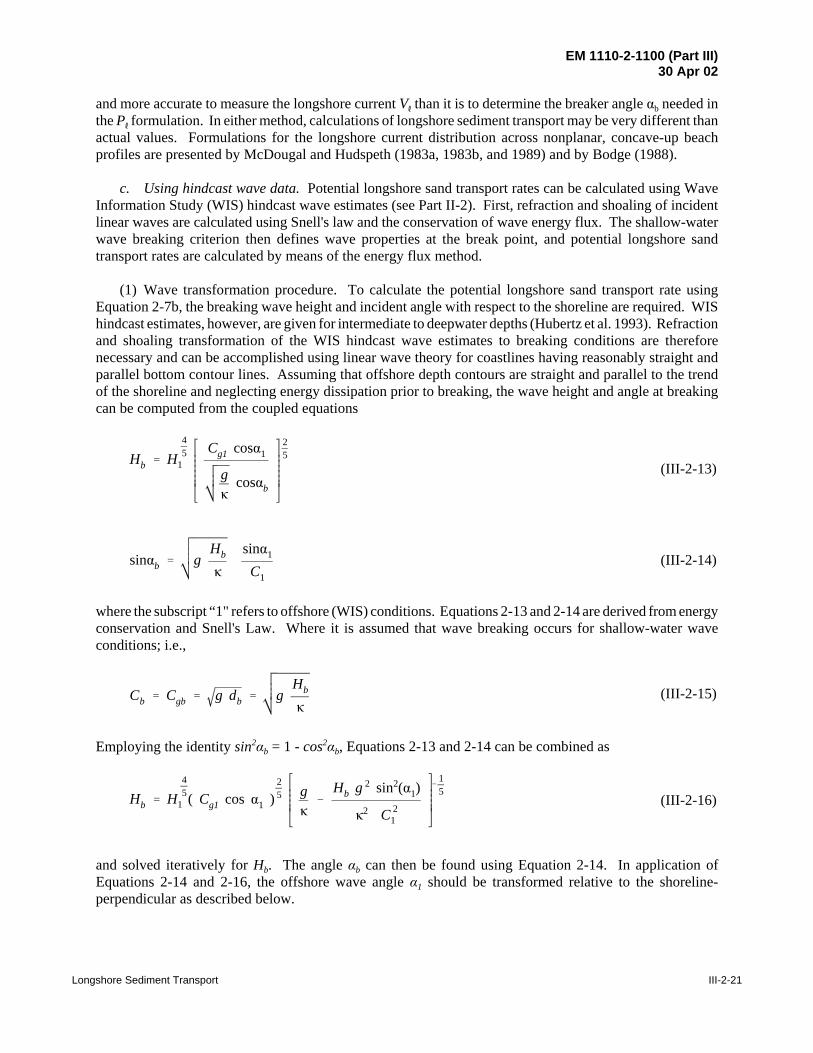
EM 1110-2-1100 (Part III)30 Apr 02
Longshore Sediment Transport III-2-21
Hb ' H45
1Cg1 cosα1
gκ
cosαb
25
(III-2-13)
sinαb ' gHb
κsinα1
C1(III-2-14)
Cb ' Cgb ' g db ' gHb
κ(III-2-15)
Hb ' H45
1 ( Cg1 cos α1 )25 g
κ&
Hb g 2 sin2(α1)
κ2 C 21
&15
(III-2-16)
and more accurate to measure the longshore current VR than it is to determine the breaker angle αb needed inthe PR formulation. In either method, calculations of longshore sediment transport may be very different thanactual values. Formulations for the longshore current distribution across nonplanar, concave-up beachprofiles are presented by McDougal and Hudspeth (1983a, 1983b, and 1989) and by Bodge (1988).
c. Using hindcast wave data. Potential longshore sand transport rates can be calculated using WaveInformation Study (WIS) hindcast wave estimates (see Part II-2). First, refraction and shoaling of incidentlinear waves are calculated using Snell's law and the conservation of wave energy flux. The shallow-waterwave breaking criterion then defines wave properties at the break point, and potential longshore sandtransport rates are calculated by means of the energy flux method.
(1) Wave transformation procedure. To calculate the potential longshore sand transport rate usingEquation 2-7b, the breaking wave height and incident angle with respect to the shoreline are required. WIShindcast estimates, however, are given for intermediate to deepwater depths (Hubertz et al. 1993). Refractionand shoaling transformation of the WIS hindcast wave estimates to breaking conditions are thereforenecessary and can be accomplished using linear wave theory for coastlines having reasonably straight andparallel bottom contour lines. Assuming that offshore depth contours are straight and parallel to the trendof the shoreline and neglecting energy dissipation prior to breaking, the wave height and angle at breakingcan be computed from the coupled equations
where the subscript “1" refers to offshore (WIS) conditions. Equations 2-13 and 2-14 are derived from energyconservation and Snell's Law. Where it is assumed that wave breaking occurs for shallow-water waveconditions; i.e.,
Employing the identity sin2αb = 1 - cos2αb, Equations 2-13 and 2-14 can be combined as
and solved iteratively for Hb. The angle αb can then be found using Equation 2-14. In application ofEquations 2-14 and 2-16, the offshore wave angle α1 should be transformed relative to the shoreline-perpendicular as described below.

EM 1110-2-1100 (Part III)30 Apr 02
III-2-22 Longshore Sediment Transport
α ' θn & WIS angle (III-2-17)
(2) Wave conditions.
(a) As discussed in Part II-2, WIS hindcast wave estimates are compiled in intermediate to deepwaterdepths. The examples presented herein use Revised Atlantic Level 2 (RAL2) WIS data, which are presentedin 45-deg wave angle bands. Angles reported for RAL2 WIS Phase III stations αWIS are measured in degrees“from” in a compass sense, for which due north equals zero and other angles are measured clockwise fromnorth. For calculation of longshore sand transport, a right-handed coordinate system is more convenient, inwhich waves approaching normal to the shoreline are given an angle of 0 deg. Looking seaward, wavesapproaching from the right are associated with negative angles, and waves approaching from the left areassociated with positive angles such that transport directed to the right is given a positive value and transportdirected to the left is given a negative value in accord with sign convention discussed earlier. WIS anglesmay be converted to angles associated with transport calculations α by means of the following relationship:
where θn is the azimuth angle of the outward normal to the shoreline. Angles of α over ± 900 would beexcluded from calculations. The WIS angle is the azimuth angle the waves are coming from.
(b) RAL2 WIS wave data for one particular wave-angle band are summarized in Table III-2-2. Thenumber of occurrences are listed for specific wave height and period bands, with the total number ofoccurrences listed in the right column (for each wave band) and bottom row (for each period band). Theheader gives the time period for the data record (1956 - 1975), location of the station in latitude and longitude,water depth, and angle band represented by the tabulated data.
(c) Data given in WIS statistical tables may be used in several ways to calculate the potential longshoresand transport rate. Two examples using the data in Table III-2-2 are given below. In Example III-2-5, thepotential longshore sand transport rate is estimated with the average significant wave height for the given
Table III-2-2Occurrence of Wave Height and Period for Direction Band 112.5E - 157.49E RAL2 Station 72
WIS ATLANTIC REVISION 1956 - 1975LAT: 40.25 N LONG: 73.75 W, DEPTH = 27 M
OCCURRENCES OF WAVE HEIGHT AND PEAK PERIODFOR 45-DEG DIRECTION BAND
STATION 72(112.500 to 157.490) mean = 135.00
Tp, secondsHmo(m) 3.0-4.9 5.0-6.9 7.0-8.9 9.0-10.9 11.0-12.9 13.0-14.9 15.0-16.9 17.0-18.9 Total0.00-0.99 1,022 1,509 6,018 3,261 918 120 10 . 12,8581.00-1.99 124 1,380 1,437 1,095 610 127 4 . 4,7772.00-2.99 . 66 440 384 183 60 . . 1,1333.00-3.99 . . 56 140 76 16 . . 2884.00-4.99 . . . 17 22 6 . . 455.00-5.99 . . . 1 2 . . . 36.00-6.99 . . . . 1 1 . . 27.00-7.99 . . . . . . . . 08.00-8.99 . . . . . . . . 09.00-Greater . . . . . . . . 0Total 1,146 2,955 7,951 4,898 1,812 330 14 0 19,106
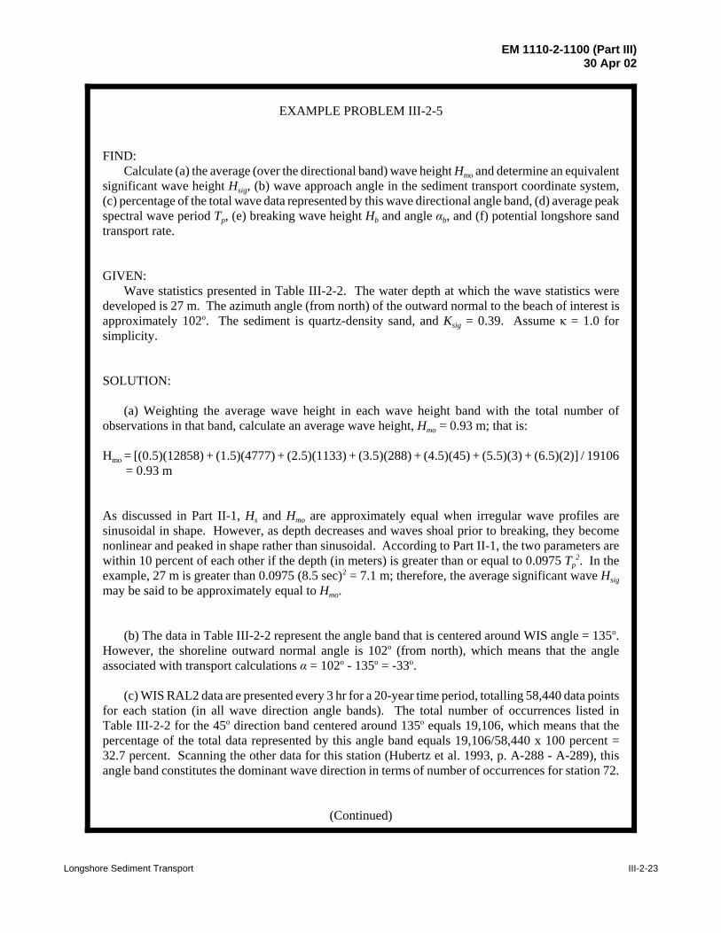
EM 1110-2-1100 (Part III)30 Apr 02
Longshore Sediment Transport III-2-23
EXAMPLE PROBLEM III-2-5
FIND:Calculate (a) the average (over the directional band) wave height Hmo and determine an equivalent
significant wave height Hsig, (b) wave approach angle in the sediment transport coordinate system,(c) percentage of the total wave data represented by this wave directional angle band, (d) average peakspectral wave period Tp, (e) breaking wave height Hb and angle αb, and (f) potential longshore sandtransport rate.
GIVEN:Wave statistics presented in Table III-2-2. The water depth at which the wave statistics were
developed is 27 m. The azimuth angle (from north) of the outward normal to the beach of interest isapproximately 102o. The sediment is quartz-density sand, and Ksig = 0.39. Assume κ = 1.0 forsimplicity.
SOLUTION:
(a) Weighting the average wave height in each wave height band with the total number ofobservations in that band, calculate an average wave height, Hmo = 0.93 m; that is:
Hmo = [(0.5)(12858) + (1.5)(4777) + (2.5)(1133) + (3.5)(288) + (4.5)(45) + (5.5)(3) + (6.5)(2)] / 19106= 0.93 m
As discussed in Part II-1, Hs and Hmo are approximately equal when irregular wave profiles aresinusoidal in shape. However, as depth decreases and waves shoal prior to breaking, they becomenonlinear and peaked in shape rather than sinusoidal. According to Part II-1, the two parameters arewithin 10 percent of each other if the depth (in meters) is greater than or equal to 0.0975 Tp
2. In theexample, 27 m is greater than 0.0975 (8.5 sec)2 = 7.1 m; therefore, the average significant wave Hsigmay be said to be approximately equal to Hmo.
(b) The data in Table III-2-2 represent the angle band that is centered around WIS angle = 135o.However, the shoreline outward normal angle is 102o (from north), which means that the angleassociated with transport calculations α = 102o - 135o = -33o.
(c) WIS RAL2 data are presented every 3 hr for a 20-year time period, totalling 58,440 data pointsfor each station (in all wave direction angle bands). The total number of occurrences listed inTable III-2-2 for the 45o direction band centered around 135o equals 19,106, which means that thepercentage of the total data represented by this angle band equals 19,106/58,440 x 100 percent =32.7 percent. Scanning the other data for this station (Hubertz et al. 1993, p. A-288 - A-289), thisangle band constitutes the dominant wave direction in terms of number of occurrences for station 72.
(Continued)
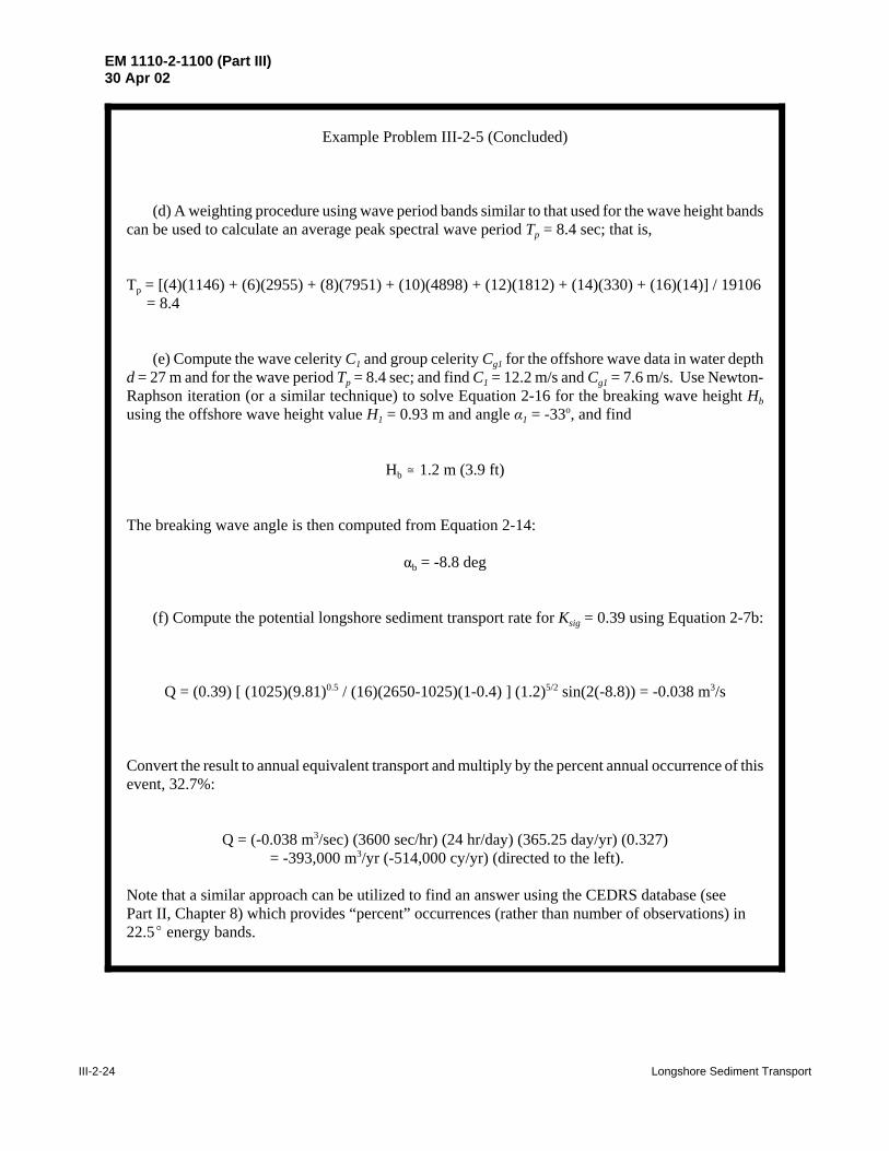
EM 1110-2-1100 (Part III)30 Apr 02
III-2-24 Longshore Sediment Transport
Example Problem III-2-5 (Concluded)
(d) A weighting procedure using wave period bands similar to that used for the wave height bandscan be used to calculate an average peak spectral wave period Tp = 8.4 sec; that is,
Tp = [(4)(1146) + (6)(2955) + (8)(7951) + (10)(4898) + (12)(1812) + (14)(330) + (16)(14)] / 19106 = 8.4
(e) Compute the wave celerity C1 and group celerity Cg1 for the offshore wave data in water depthd = 27 m and for the wave period Tp = 8.4 sec; and find C1 = 12.2 m/s and Cg1 = 7.6 m/s. Use Newton-Raphson iteration (or a similar technique) to solve Equation 2-16 for the breaking wave height Hbusing the offshore wave height value H1 = 0.93 m and angle α1 = -33o, and find
Hb – 1.2 m (3.9 ft)
The breaking wave angle is then computed from Equation 2-14:
αb = -8.8 deg
(f) Compute the potential longshore sediment transport rate for Ksig = 0.39 using Equation 2-7b:
Q = (0.39) [ (1025)(9.81)0.5 / (16)(2650-1025)(1-0.4) ] (1.2)5/2 sin(2(-8.8)) = -0.038 m3/s
Convert the result to annual equivalent transport and multiply by the percent annual occurrence of thisevent, 32.7%:
Q = (-0.038 m3/sec) (3600 sec/hr) (24 hr/day) (365.25 day/yr) (0.327) = -393,000 m3/yr (-514,000 cy/yr) (directed to the left).
Note that a similar approach can be utilized to find an answer using the CEDRS database (seePart II, Chapter 8) which provides “percent” occurrences (rather than number of observations) in22.5E energy bands.

EM 1110-2-1100 (Part III)30 Apr 02
Longshore Sediment Transport III-2-25
EXAMPLE PROBLEM III-2-6FIND:
Calculate the potential longshore transport rate using each of the seven wave height bands given inTable III-2-2.
GIVEN:Data in Table III-2-2, and information in Example III-2-5.
SOLUTION:For each wave height band in Table III-2-2, the associated weighted average peak wave period Tp is
calculated. Using the criteria discussed previously, the wave data are checked to ensure that Hsig ~ Hmo.The percent occurrence for that wave condition is determined by dividing the total number of occurrencesin the wave height band in the given 450 directional band by the total number of records (58,440) in alldirectional bands. The results are shown in the table below as the “input” conditions. The breakingconditions may be computed directly by the program WISTRT or by Equations 2-14 and 2-16 in the samemanner as described in Example 5, above. The potential longshore sediment transport from the 45o
direction band centered approximately 33o to the right of shore-normal (looking seaward) was calculatedto be -1,014,200 m3/year (-1,325,500 yd3/year) (directed to the left) for RAL2 Station 72.
Data for Example Problem III-2-6
Input Conditions Program Output
WaveCondition
Hs(m)
T(sec)
α(deg)
Depth(m)
PercentOccurrence
Hb(m)
αb(deg)
QR
(m3/year)
1 0.5 8.3 -33 27 22.0 0.73 -7.8 -66,500
2 1.5 8.5 -33 27 8.17 1.8 -12.0 -355,000
3 2.5 9.5 -33 27 1.94 2.9 -14.2 -320,000
4 3.5 10.4 -33 27 0.493 4.0 -16.0 -198,800
5 4.5 11.5 -33 27 0.077 5.1 -17.4 -61,200
6 5.5 11.3 -33 27 0.005 6.0 -19.0 -6,500
7 6.5 13.0 -33 27 0.003 7.1 -20.0 -6,200
Total (directed to the left) -1,014,200
Note that a similar approach can be utilized to find an answer using the CEDRS database (seePart II, Chapter 8) which provides “percent” occurrences (rather than number of observations) in22.5E energy bands. Note that engineering judgment must be utilized when assessing actualtransport rates. Values of longshore sand transport calculated with Equations 2-14 and 2-16 arebased on a limitless supply of sand available for transport, which is often not the case (e.g., ifstructures are present, geologic features control sand movement, or sediments other than sandare in the transport region). In addition, longshore transport rates calculated using WIS datahave been found to be larger than accepted rates (Bodge and Kraus 1991).For this example calculated using waves offshore of the New Jersey coast, generally-acceptedtransport rates might be used to adjust the calculated values. Inspection of Figure III-2-3indicates that net longshore transport rates are between 153,000 and 275,000 cu m/year for thisportion of the New Jersey shore. This “calibration” implies that longshore sand transport ratescalculated with WIS data and Equations 2-14 and 2-16 might be reduced from 15 to 27 percentof their calculated values to have application for this part of the coastline. Future calculationsusing WIS data for this portion of the coast could use this calibration for adjustment.

EM 1110-2-1100 (Part III)30 Apr 02
III-2-26 Longshore Sediment Transport
QRNET / Q R'
1To m
To
o
QR (t)dt (III-2-18)
directional band. In Example III-2-6, wave data are more accurately represented by calculating arepresentative wave period for each of the given wave height bands for the given directional band. Eachexample requires the transformation of offshore wave data to breaking conditions, and subsequentcomputation of the associated longshore transport rate. The former can be accomplished usingEquations 2-14 and 2-16 or using the program WISTRT (Gravens 1989). Both require knowledge or inputof the offshore wave height H1 (WISTRT requires the significant wave height Hsig), associated period T, anglerelative to the shoreline α, and water depth associated with wave data. The longshore transport rate can thenbe computed directly by Equation 2-7b. The program WISTRT uses a K value and a breaker wave height-to-depth ratio different than those used here. It also requires the percent occurrence associated with the givenwave condition. The ACES program “Longshore Sediment Transport” (Leenknecht, Szuwalski, and Sherlock1992) also provides a method for calculation of potential longshore sediment transport rates under the actionof waves. Again, different constants K and κ are utilized than those presented here. Both WISTRT and theACES programs use individual wave events as input, rather than an extended time series of wave information.A program for processing the WIS time series to obtain values of sediment transport is presented in Gravens,Kraus, and Hanson (1991).
(d) Note that both Examples III-2-5 and III-2-6 employed the same wave data, but Example III-2-6computed the transport for discrete wave height bands whereas Example III-2-5 computed the transport fora single, band-averaged wave height. The transport computed in Example III-2-6 is more than double thatin Example III-2-5. This difference is due to the nonlinear dependence of the transport equation on breakingwave height. If, for example, wave heights are Rayleigh distributed and the waves are all of uniform period,the transport rate computed using the distribution of wave heights will be about 1.53 times larger than thatcomputed using only the band-averaged wave height.
(e) Bodge and Kraus (1991) and others (e.g., Kraus and Harikai 1983; Gravens, Scheffner, and Hubertz1989; Gravens 1990a) have observed that use of the CERC formula (with the KSPM coefficient) and WIShindcast wave data have yielded potential longshore sand transport magnitudes that are two to five timeslarger than values for the region as estimated from dredging records, bypassing rates, or volumetric change.The longshore sand transport rate determined in Example III-2-6 represents the potential longshore transportrate, which depends on an available supply of littoral material. Consideration of the availability of littoralmaterial; location, type, and condition of coastal structures; and sheltering specific to the project shorelinemay contribute to a lower actual longshore transport rate. It is recommended when using hindcast wave datato predict potential longshore sand transport rates that other independent measures or estimates of longshoretransport be used to supplement the potential transport estimate.
d. Deviation from potential longshore sediment transport rates.
(1) Temporal variations and persistence.
(a) Longshore sediment transport is a fluctuating quantity which can be depicted as shown inFigure III-2-7 where positive sediment transport is defined as positive in value if toward the right for anobserver looking seaward from the beach, and negative in value if sediment transport is toward the left asnoted previously and consistent with notation utilized by Walton (1972), Walton and Dean (1973), Dean(1987), and others. In terms of “QR,” on Figure III-2-7 the net longshore sediment transport rate is the “timeaverage” transport given by

EM 1110-2-1100 (Part III)30 Apr 02
Longshore Sediment Transport III-2-27
Figure III-2-7. Longshore transport definitions
QRGROSS '1To m
To
o
*QR (t)*dt (III-2-19)
(b) The gross longshore sediment transport rate is given by
where To is the length of record, often taken to be greater than 1 year, and |QR| is the absolute magnitude ofthe longshore sediment transport rate. The gross longshore sediment transport rate is always defined positive.When the gross longshore sediment transport rate is multiplied by the time period, the derived quantityrepresents the total volume of sediment passing through a plane perpendicular to the shoreline regardless ofthe direction. The net longshore sediment transport rate may be either positive or negative.
(c) Although net and gross longshore sediment transport rates are often the most meaningful quantitiesfor use in engineering design, the variability of the longshore sediment transport on much shorter timeintervals is often of critical concern. As an example, if a channel is to be maintained clear of sediment, thepump(s) necessary to dredge the channel would need to be sufficiently large to handle the instantaneousmaximum rate of longshore rate of sediment transport (that is projected to reach the channel). Typically,sizing for the maximum instantaneous rate of sediment transport would be economically unfeasible, andtherefore some type of temporary sediment storage would be provided to allow for reduced pump sizing.Optimizing of the pump size and the provided sediment storage structures (possibly a groin, a breakwater,or some combination of both) will require knowledge of the fluctuating longshore sediment transportrates.Figure III-2-8 provides an example of the variability of annual rates of (net) longshore energy flux factor(which is proportional to the longshore sediment transport rate as given in Equation 2-2) for three locationson the East Coast of the United States as computed using 20 years of hindcast wave climate.

EM 1110-2-1100 (Part III)30 Apr 02
III-2-28 Longshore Sediment Transport
Figure III-2-8. Time plot of annual longshore energy flux factor at three east coast sites (after Douglass(1985))
Figure III-2-9 provides an example of the variability of the monthly (net) longshore energy flux factor forthe same three locations. Figures III-2-8 and III-2-9 show that as the averaging period gets shorter, thevariability of the sediment transport rate increases due to the fact that integration is a smoothing process andreduces the variance in the data. For design purposes, an assessment of the uncertainty in the sedimenttransport climate can be addressed via simulation of the sediment transport rates. Walton and Douglass(1985) have provided an approach to such simulation for the case of monthly sand transport rates which, forthe locations assessed, appeared to be in reasonable conformance with a normal distribution assumption.Figure III-2-10 from Walton and Douglass (1985) shows the distribution of monthly averages of longshoreenergy flux factor for a coastal location in South Carolina. The data are reasonably represented by a normaldistribution, as shown by the fit of the solid line to the data. Figure III-2-11, also from Walton and Douglass(1985), is for the same location but with weekly averages. In this case, the weekly averages vary considerablyfrom a normal probability distribution.

EM 1110-2-1100 (Part III)30 Apr 02
Longshore Sediment Transport III-2-29
Figure III-2-9. Time plot of monthly longshore energy flux factor time series for 1956-1975 at three eastcoast sites (after Douglass (1985))
E' -u; / Ill _J
t '--'
en ...... 11..
E' / (/)
/ Ill _J
I
~ en ......
a..
E' / (/)
/ Ill _J
I
~ en ...
11..
1000 ~
500 -
0
-500 f-
1/56
I ~~
MURRELLS INLET, SC
OCEAN CITY, MD
IU Ill I~ II II .I II wiJ PONCE DE LEON INLET, FL
I •11 II l II 1"
I
TIME 12/75

EM 1110-2-1100 (Part III)30 Apr 02
III-2-30 Longshore Sediment Transport
Figure III-2-11. Probability plot for weekly average Pls series (Walton and Douglass 1985)
Figure III-2-10. Probability plot for monthly average Pls series (Walton and Douglass 1985)
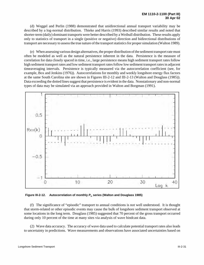
EM 1110-2-1100 (Part III)30 Apr 02
Longshore Sediment Transport III-2-31
Figure III-2-12. Autocorrelation of monthly Pls series (Walton and Douglass 1985)
(d) Weggel and Perlin (1988) demonstrated that unidirectional annual transport variability may bedescribed by a log-normal distribution. Thieke and Harris (1993) described similar results and noted thatshorter-term (daily) dominant transports were better described by a Weibull distribution. These results applyonly to statistics of transport in a single (positive or negative) direction and bidirectional distributions oftransport are necessary to assess the true nature of the transport statistics for proper simulation (Walton 1989).
(e) When assessing various design alternatives, the proper distribution of the sediment transport rate mustoften be modeled as well as the natural persistence inherent in the data. Persistence is the measure ofcorrelation for data closely spaced in time, i.e., large persistence means high sediment transport rates followhigh sediment transport rates and low sediment transport rates follow low sediment transport rates in adjacenttimeaveraging intervals. Persistence is typically measured via the autocorrelation coefficient (see, forexample, Box and Jenkins (1976)). Autocorrelations for monthly and weekly longshore energy flux factorsat the same South Carolina site are shown in Figures III-2-12 and III-2-13 (Walton and Douglass (1985)).Data exceeding the dotted lines suggest that persistence is evident in the data. Nonstationary and non-normaltypes of data may be simulated via an approach provided in Walton and Borgman (1991).
(f) The significance of “episodic” transport to annual conditions is not well understood. It is thoughtthat storm-related or other episodic events may cause the bulk of longshore sediment transport observed atsome locations in the long term. Douglass (1985) suggested that 70 percent of the gross transport occurredduring only 10 percent of the time at many sites via analysis of wave hindcast data.
(2) Wave data accuracy. The accuracy of wave data used to calculate potential transport rates also leadsto uncertainty in predictions. Wave measurements and observations have associated uncertainties based on
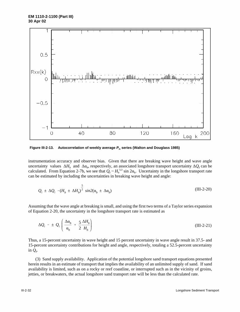
EM 1110-2-1100 (Part III)30 Apr 02
III-2-32 Longshore Sediment Transport
Figure III-2-13. Autocorrelation of weekly average Pls series (Walton and Douglass 1985)
QR ± ∆QR -(Hb ± ∆Hb)52 sin2(αb ± ∆αb) (III-2-20)
∆QR - ± QR
∆αb
αb
%52∆Hb
Hb(III-2-21)
instrumentation accuracy and observer bias. Given that there are breaking wave height and wave angleuncertainty values ∆Hb and ∆αb, respectively, an associated longshore transport uncertainty ∆QR can becalculated. From Equation 2-7b, we see that QR ~ Hb
5/2 sin 2αb. Uncertainty in the longshore transport ratecan be estimated by including the uncertainties in breaking wave height and angle:
Assuming that the wave angle at breaking is small, and using the first two terms of a Taylor series expansionof Equation 2-20, the uncertainty in the longshore transport rate is estimated as
Thus, a 15-percent uncertainty in wave height and 15 percent uncertainty in wave angle result in 37.5- and15-percent uncertainty contributions for height and angle, respectively, totaling a 52.5-percent uncertaintyin QR.
(3) Sand supply availability. Application of the potential longshore sand transport equations presentedherein results in an estimate of transport that implies the availability of an unlimited supply of sand. If sandavailability is limited, such as on a rocky or reef coastline, or interrupted such as in the vicinity of groins,jetties, or breakwaters, the actual longshore sand transport rate will be less than the calculated rate.
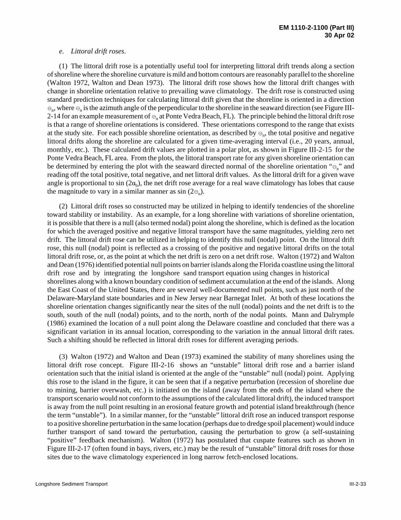
EM 1110-2-1100 (Part III)30 Apr 02
Longshore Sediment Transport III-2-33
e. Littoral drift roses.
(1) The littoral drift rose is a potentially useful tool for interpreting littoral drift trends along a sectionof shoreline where the shoreline curvature is mild and bottom contours are reasonably parallel to the shoreline(Walton 1972, Walton and Dean 1973). The littoral drift rose shows how the littoral drift changes withchange in shoreline orientation relative to prevailing wave climatology. The drift rose is constructed usingstandard prediction techniques for calculating littoral drift given that the shoreline is oriented in a directionsn, where sn is the azimuth angle of the perpendicular to the shoreline in the seaward direction (see Figure III-2-14 for an example measurement of sn at Ponte Vedra Beach, FL). The principle behind the littoral drift roseis that a range of shoreline orientations is considered. These orientations correspond to the range that existsat the study site. For each possible shoreline orientation, as described by sn, the total positive and negativelittoral drifts along the shoreline are calculated for a given time-averaging interval (i.e., 20 years, annual,monthly, etc.). These calculated drift values are plotted in a polar plot, as shown in Figure III-2-15 for thePonte Vedra Beach, FL area. From the plots, the littoral transport rate for any given shoreline orientation canbe determined by entering the plot with the seaward directed normal of the shoreline orientation “sn” andreading off the total positive, total negative, and net littoral drift values. As the littoral drift for a given waveangle is proportional to sin (2αb), the net drift rose average for a real wave climatology has lobes that causethe magnitude to vary in a similar manner as sin (2sn).
(2) Littoral drift roses so constructed may be utilized in helping to identify tendencies of the shorelinetoward stability or instability. As an example, for a long shoreline with variations of shoreline orientation,it is possible that there is a null (also termed nodal) point along the shoreline, which is defined as the locationfor which the averaged positive and negative littoral transport have the same magnitudes, yielding zero netdrift. The littoral drift rose can be utilized in helping to identify this null (nodal) point. On the littoral driftrose, this null (nodal) point is reflected as a crossing of the positive and negative littoral drifts on the totallittoral drift rose, or, as the point at which the net drift is zero on a net drift rose. Walton (1972) and Waltonand Dean (1976) identified potential null points on barrier islands along the Florida coastline using the littoraldrift rose and by integrating the longshore sand transport equation using changes in historicalshorelines along with a known boundary condition of sediment accumulation at the end of the islands. Alongthe East Coast of the United States, there are several well-documented null points, such as just north of theDelaware-Maryland state boundaries and in New Jersey near Barnegat Inlet. At both of these locations theshoreline orientation changes significantly near the sites of the null (nodal) points and the net drift is to thesouth, south of the null (nodal) points, and to the north, north of the nodal points. Mann and Dalrymple(1986) examined the location of a null point along the Delaware coastline and concluded that there was asignificant variation in its annual location, corresponding to the variation in the annual littoral drift rates.Such a shifting should be reflected in littoral drift roses for different averaging periods.
(3) Walton (1972) and Walton and Dean (1973) examined the stability of many shorelines using thelittoral drift rose concept. Figure III-2-16 shows an “unstable” littoral drift rose and a barrier islandorientation such that the initial island is oriented at the angle of the “unstable” null (nodal) point. Applyingthis rose to the island in the figure, it can be seen that if a negative perturbation (recession of shoreline dueto mining, barrier overwash, etc.) is initiated on the island (away from the ends of the island where thetransport scenario would not conform to the assumptions of the calculated littoral drift), the induced transportis away from the null point resulting in an erosional feature growth and potential island breakthrough (hencethe term “unstable”). In a similar manner, for the “unstable” littoral drift rose an induced transport responseto a positive shoreline perturbation in the same location (perhaps due to dredge spoil placement) would inducefurther transport of sand toward the perturbation, causing the perturbation to grow (a self-sustaining“positive” feedback mechanism). Walton (1972) has postulated that cuspate features such as shown inFigure III-2-17 (often found in bays, rivers, etc.) may be the result of “unstable” littoral drift roses for thosesites due to the wave climatology experienced in long narrow fetch-enclosed locations.

EM 1110-2-1100 (Part III)30 Apr 02
III-2-34 Longshore Sediment Transport
Figure III-2-14. Azimuth of normal to shoreline at Ponte Vedra Beach, Florida (Walton 1972)
(4) Another possibility is that the littoral drift rose along a shoreline is as shown in Figure III-2-18. Inthis case the null (nodal) point is stable. Perturbations in the shoreline, positive (accretions) or negative(recessions), now result in transport which tends to reduce rather than accentuate the perturbation(a “negative” feedback mechanism). In this case there is not a self-sustaining tendency toward islandbreaching Walton (1972) noted that the east coast of Florida is characterized by this type of littoral drift roseand, in fact, there are relatively few natural inlets along this coastline and a historical tendency of those inletsthat are opened by man to close (unless closure is prevented via coastal structures such as jetties).

EM 1110-2-1100 (Part III)
30 Apr 02
Longshore Sediment Transport
III-2-35
Figure III-2-15. Net and total littoral drift at Ponte Vedra Beach, Florida (Walton 1972)
?.NNUALL Y AVU(A.GED i'iLT UTTOI;:AL Dl~!l 1
N ICY
z ('I"! __,
800 0 !! 700 "T] __,
z. 600
C> 500 c: UJ 0 400 -< :soo )> ;::o C:J
200 (J)
L1 fTJ 100 ;::o
0
~
180' 170" - r~r~t
.................... Net
NJNUALLY AVmACLD TOTAL UTTOf\i:..L UF~ill
__, N 10" Cl
I
0 1600 ;u j 1400
z 12CJC n c:· 1000 ClJ :"i
8DCJ <
)> 600 ;:.!)
0 (f)
8f} 400 u ["1'1
;{) 200 CJ
90" .1<
1 ()()'
180' 170"
[lirection Direction
70'
9U
100"
110a
rotc I ...................................... TotCJi
Dirccti(1n Directi(Jn

EM 1110-2-1100 (Part III)30 Apr 02
III-2-36 Longshore Sediment Transport
Figure III-2-16. Ideal case of an unstable null point (Walton 1972)
f. Cross-shore distribution of longshore sediment transport.
(1) The relationships given herein yield rates of total longshore sediment transport. Some applicationsrequire evaluations of the cross-shore distribution of the transport; e.g., for the effective design of groins,jetties, and sand weirs for weir jetties. In addition, a description of the cross-shore transport distribution isrequired in many computer simulation models.
(2) Bodge (1986) presents a literature review of the data and models which describe the cross-shoredistribution of the longshore sediment transport. The collection of field data regarding this topic is difficult.The earliest approach was to use sand tracers (e.g., Zenkovitch 1960; Ingle 1966; Inman, Komar, and Bowen1968; Inman, Tait, and Nordstrom 1971; Inman et al. 1980; Kraus et al. 1982, White 1987). As an example,Zenkovitch (1960) determined distributions at a coastal site by averaging a large number of tracerobservations and found three maxima for the sand transport: two over longshore bars and a third in the swash

EM 1110-2-1100 (Part III)30 Apr 02
Longshore Sediment Transport III-2-37
Figure III-2-17. Instability-formed capes in Santa Rosa Sound (Walton 1972)
zone. Ingle (1966) used fluorescent-dyed sediment at five test sites along the California coast to investigatethe longshore rate of tracer dispersion, as well as its cross-shore distribution. An example of the cross-shoredistribution of tracer density measured at Goleta Point in October 1961 is shown at three measurementintervals for two surf zone cross-sections in Figure III-2-19. Cross-section A represents conditions 46 m(150 ft) downdrift of the release line, and cross-section B is 46 m (150 ft) downdrift of cross-section A. Thedistributions indicate that the most rapid tracer dispersal took place at the edge of the swash zone, while thegreatest tracer transport took place at the breaker zone.
(3) Using sediment traps operated from a Florida pier across the outer portion of the surf zone, Thornton(1972) found that longshore transport was a maximum on the seaward side of the longshore bar where waveswere breaking. Sawaragi and Deguchi (1978) placed round sediment traps divided into pie-shaped sectionsinto the beach and found three basic longshore transport distribution profiles: (1) maximum in the swash zoneor near the shoreline, (2) maximum at the breaker line, and (3) bimodal with maxima at the shore and breakerlines. From a field study using fluorescent tracers, Kraus et al. (1982) likewise observed similar results inaddition to a generally uniform cross-shore distribution. Berek and Dean (1982) inferred longshore transportdistribution from measurements of contour rotation in a pocket beach at Santa Barbara, California, and foundfrom their data that the transport was greatest across the inner surf zone. Kraus and Dean (1987) and Kraus,Gingerich, and Rosati (1989) give general examples of vertical and cross-shore distributions of longshoresediment flux measured with portable traps (see Figure III-2-2).

EM 1110-2-1100 (Part III)30 Apr 02
III-2-38 Longshore Sediment Transport
Figure III-2-18. Ideal case of a stable null point (Walton 1972)
(4) Kana (1978) measured the vertical suspended sediment concentration at locations across the surfzone, and longshore current velocity at a mid-surf position. His measurements indicated that, for spillingwaves, sediment concentration rapidly increased inside the breakpoint, then remained relatively constantunder the bore as it propagated towards the beach. For plunging waves, sediment concentration peaked

EM 1110-2-1100 (Part III)30 Apr 02
Longshore Sediment Transport III-2-39
Figure III-2-19. Distribution of tracer density across the surf zone, 20 October 1961 Goleta Point,California, experiment (Ingle 1966)
within a few meters of the breakpoint, then decreased gradually towards shore (see Figure III-2-20).Downing (1984) and Sternberg, Shi, and Downing (1984) likewise measured vertical sediment concentrationprofiles simultaneously with the longshore current, and found maximum transport at about the mid-surf-zonelocation. The measurements did not include the inshore portion of the surf zone and did not account for bed-load transport.
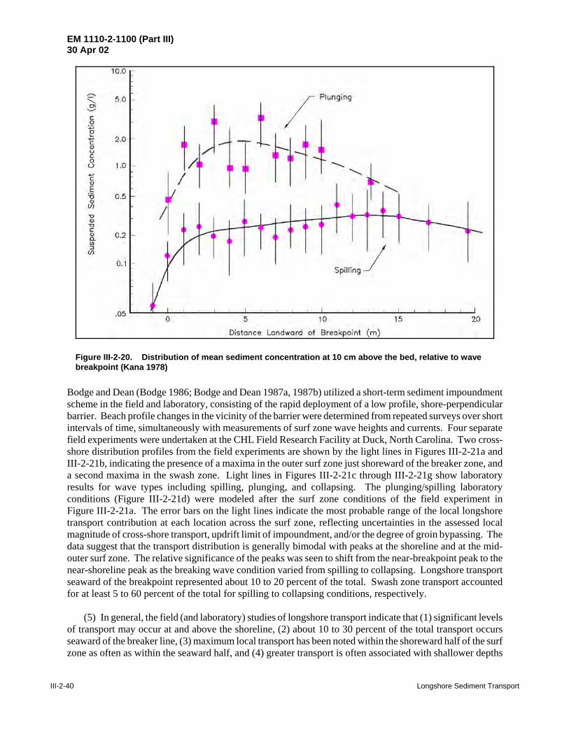
EM 1110-2-1100 (Part III)30 Apr 02
III-2-40 Longshore Sediment Transport
Figure III-2-20. Distribution of mean sediment concentration at 10 cm above the bed, relative to wavebreakpoint (Kana 1978)
Bodge and Dean (Bodge 1986; Bodge and Dean 1987a, 1987b) utilized a short-term sediment impoundmentscheme in the field and laboratory, consisting of the rapid deployment of a low profile, shore-perpendicularbarrier. Beach profile changes in the vicinity of the barrier were determined from repeated surveys over shortintervals of time, simultaneously with measurements of surf zone wave heights and currents. Four separatefield experiments were undertaken at the CHL Field Research Facility at Duck, North Carolina. Two cross-shore distribution profiles from the field experiments are shown by the light lines in Figures III-2-21a andIII-2-21b, indicating the presence of a maxima in the outer surf zone just shoreward of the breaker zone, anda second maxima in the swash zone. Light lines in Figures III-2-21c through III-2-21g show laboratoryresults for wave types including spilling, plunging, and collapsing. The plunging/spilling laboratoryconditions (Figure III-2-21d) were modeled after the surf zone conditions of the field experiment inFigure III-2-21a. The error bars on the light lines indicate the most probable range of the local longshoretransport contribution at each location across the surf zone, reflecting uncertainties in the assessed localmagnitude of cross-shore transport, updrift limit of impoundment, and/or the degree of groin bypassing. Thedata suggest that the transport distribution is generally bimodal with peaks at the shoreline and at the mid-outer surf zone. The relative significance of the peaks was seen to shift from the near-breakpoint peak to thenear-shoreline peak as the breaking wave condition varied from spilling to collapsing. Longshore transportseaward of the breakpoint represented about 10 to 20 percent of the total. Swash zone transport accountedfor at least 5 to 60 percent of the total for spilling to collapsing conditions, respectively.
(5) In general, the field (and laboratory) studies of longshore transport indicate that (1) significant levelsof transport may occur at and above the shoreline, (2) about 10 to 30 percent of the total transport occursseaward of the breaker line, (3) maximum local transport has been noted within the shoreward half of the surfzone as often as within the seaward half, and (4) greater transport is often associated with shallower depths
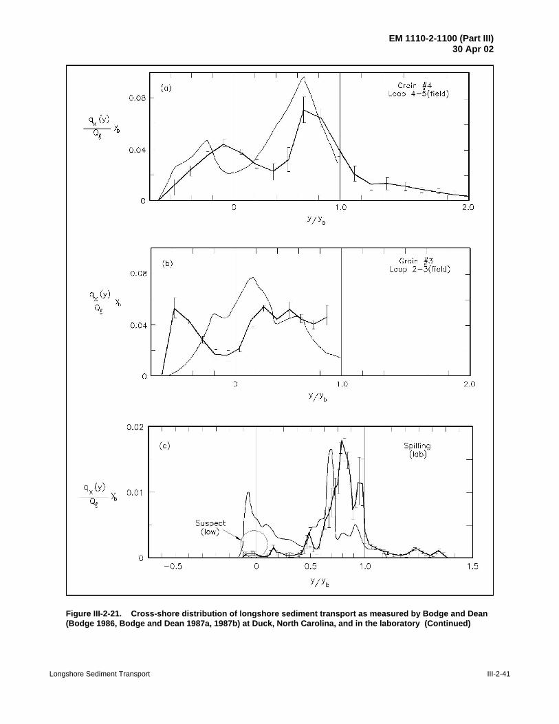
EM 1110-2-1100 (Part III)30 Apr 02
Longshore Sediment Transport III-2-41
Figure III-2-21. Cross-shore distribution of longshore sediment transport as measured by Bodge and Dean(Bodge 1986, Bodge and Dean 1987a, 1987b) at Duck, North Carolina, and in the laboratory (Continued)
(b) 0.08
0.04
0
0.02
(c)
qx (y) 0.01 __ yt>
Qt
Suspect (low)
0 -0.5
0 1.0
y jYb
0 0.5
YjYb
1.0
Groin #3 Loop 2-3(field)
Spilling (lab)
2.0
1.5

EM 1110-2-1100 (Part III)30 Apr 02
III-2-42 Longshore Sediment Transport
Figure III-2-21. (Concluded)
qx( Y) y --we b
qx( Y) y --we b
qx( Y) y --we b
qx( Y) y --we b
0.03
0.02
0.01
0
0.01
0
0.03
0.02
0.01
0
0.02
0.01
0
(d)
(e)
1.0
Plunge/Spill (Lab)
Plunging (Lab)
Plunge/Collapse (Lab)
Collapsing (Lab)
1.5

EM 1110-2-1100 (Part III)30 Apr 02
Longshore Sediment Transport III-2-43
qx(y) ' kq1d
MMx
(E Cg ) VR (III-2-22)
qx(y) ' kq18ρg
32 H
H%d2 dH
dy%
H2 (H%d)
ddy
(H%d) VR (III-2-23)
and breaking waves (i.e., breakpoint bars and the shoreline). Overall, field measurements demonstrate greatvariability in the shape of the longshore transport distribution profile across shore.
(6) Stresses exerted by waves vary in the cross-shore direction, generally decreasing from the breakerzone to the shoreline, but not necessarily in a uniform manner due to the presence of bars and troughs on thebeach profile. The longshore current also has a characteristic profile, and because sand transport is a resultof the combined waves and currents, its distribution will be related to their distributions. Theoreticalrelationships for the cross-shore distribution of longshore sediment transport have been postulated (e.g.,Bagnold 1963, Komar 1977, Walton 1979, McDougal and Hudspeth 1981, Bailard and Inman 1981);however, they have not been shown to reproduce field measurements well. Using data from their field andlaboratory experiments, Bodge and Dean tested five existing cross-shore distribution relationships, whichwere concluded to give from fair to poor correlation with measurements. Bodge and Dean based on the workof Bagnold (1963) also proposed a relationship for the cross-shore distribution of longshore sedimenttransport which assumes that sediment is mobilized in proportion to the local rate of wave energy dissipationper unit volume, and transported alongshore by an ongoing current
where qx(y) is the local longshore transport per unit width offshore, y represents the cross-shore coordinate,kq is a dimensional normalizing constant, d is the local water depth in the surf zone (including wave-inducedsetup), E represents the local wave energy density, Cg is the local wave group celerity, and VR is the locallongshore current speed. Equation 2-22 can be expanded by assuming shallow water conditions, small anglesof wave incidence, and assuming a nonlinear value for Cg = (g(H+d))1/2
in which H is the local wave height in the surf zone. Equation 2-23 represents conditions landward of thebreakpoint; seaward of the breakpoint, qx(y) = 0 under the assumption that no energy dissipation occurs. Inapplication of Bodge and Dean's relationship, the dimensional constant kq may be determined by integratingthe distribution qx(y) across the surf zone, and equating this quantity to the total longshore sand transport rateQR.
(7) The model (solid lines in Figure III-2-21) was compared with field data, and predicted the generaltrend of the measured transport distribution fairly well for one case (Figure III-2-21a), but shifted the cross-shore distribution slightly shoreward relative to the measured data for the second case (Figure III-2-21b).Comparison of the model with laboratory data indicated that the model generally overpredicted transport inthe mid-surf zone (especially for the plunging/collapsing and collapsing cases) and modeled the near-shoreline transport distribution to a more reasonable degree than previous approaches.
g. Application of longshore sediment transport calculations.
(1) Littoral budgets.
(a) A littoral sediment budget reflects an application of the principle of continuity or conservation ofmass to coastal sediment. The time rate of change of sediment within a system is dependent upon the rateat which material is brought into a control volume versus the rate at which sediment leaves the same volume.The budget involves assessing the sedimentary contributions and losses and equating these to the net balanceof sediment in a coastal compartment. Any process that results in a net increase in sediment in a control

EM 1110-2-1100 (Part III)30 Apr 02
III-2-44 Longshore Sediment Transport
EXAMPLE PROBLEM III-2-7
FIND:Cross-shore distribution of longshore sediment transport using Equation 2-23.
GIVEN:Waves in 10-m (32.8-ft) depth have an rms wave height of 2.0 m (6.6 ft), angle of 10 deg to the
shoreline, and wave period 8.5 sec. The beach profile is as given below. Assume the wave height towater depth ratio for incipient breaking κ = 1.0, the stable wave height to water depth ratio for wavere-formation Γstb = 0.40, the energy flux dissipation rate γ = 0.15, the lateral mixing coefficient Λmix = 0.30,and bottom friction coefficient Cf = 0.01. The K parameter (for use in longshore transport relationships)was calculated as 0.60.
Beach profile for Example III-2-7
No. DistanceOffshore (m)
Depth(m)
1 100.0 -0.60
2 111.0 0.10
3 132.0 1.00
4 145.0 1.50
5 156.0 1.70
6 169.0 1.90
7 173.0 1.95
8 186.0 1.85
9 190.0 1.80
10 195.0 1.70
11 199.0 1.75
12 207.0 1.81
13 214.0 2.00
14 246.0 3.10
15 340.0 4.00
SOLUTION:Part II-3 presents relationships for nearshore wave transformation and Part II-4 discusses the
cross-shore distribution of nearshore currents. Alternately, the PC-based numerical model NMLONG(see Part II-4 for a complete description) may be used to calculate the cross-shore distribution of totalwater depth and longshore current speed over an irregular bottom profile (Kraus and Larson 1991),which can be used in application of Equation 2-23. Entering the given data set, with 100 computationpoints, a cross-shore spacing of 2.0 m (6.6 ft), no wind, and a tidal reference elevation of 0.0, thecross-shore distribution of waves and currents as shown in Figure III-2-22b is obtained. A reducedlisting of the NMLONG output, chosen to represent the peaks and minima of the wave height andlongshore current distributions, is presented in the first four columns of the following table. Thepredicted qx(y)/kq is shown in the last column and in Figure III-2-22a.
99Example Problem III-2-7 (Sheet 1 of 4)

EM 1110-2-1100 (Part III)30 Apr 02
Longshore Sediment Transport III-2-45
Figure III-2-22. Example III-2-7, predicted cross-shore distribution of longshore sand transport, waveheight, and longshore current speed
Example Problem III-2-7 (Continued)
Example Problem III-2-7 (Sheet 2 of 4)

EM 1110-2-1100 (Part III)30 Apr 02
III-2-46 Longshore Sediment Transport
Example Problem III-2-7 (Continued)
Output from NMLONG and Calculation of Cross-shore Distribution of LongshoreTransport for Example Problem III-2-7
Cross-shoreCoordinate
(m)
Depthd
(m)
WaveHeightH (m)
Longshorecurrent speed
(m/sec)
qx(y)/kq
(kg m2/sec4)
110 0.09 0.20 0.20 83.3
112 -0.04 0.26 0.22 41.6
114 -0.14 0.32 0.25 40.8
126 -0.66 0.67 0.39 80.4
128 -0.74 0.74 0.39 82.9
130 -0.83 0.82 0.39 99.1
132 -0.91 0.90 0.34 89.4
134 -1.00 0.98 0.26 72.0
136 -1.08 0.96 0.20 - 6.9
148 -1.52 0.90 0.05 - 0.6
150 -1.55 0.89 0.04 - 0.7
152 -1.59 0.89 0.03 0.2
160 -1.73 0.87 0.02 - 0.4
162 -1.76 0.87 0.02 0.10
164 -1.79 0.87 0.02 0.10
178 -1.93 0.85 0.07 - 0.4
180 -1.91 0.85 0.08 - 0.3
182 -1.90 0.86 0.10 2.0
204 -1.80 1.10 0.51 37.5
210 -1.84 1.14 0.54 67.0
212 -1.89 1.18 0.56 72.2
238 -2.76 1.77 0.74 149.5
240 -2.83 1.83 0.74 179.7
242 -2.89 1.88 0.74 152.6
256 -3.18 2.34 0.63 223.8
258 -3.20 2.42 0.59 215.2
260 -3.21 2.42 0.53 2.3
278 -3.39 2.39 0.19 1.5
280 -3.41 2.39 0.17 1.4
282 -3.43 2.38 0.15 - 5.2
Example Problem III-2-7 (Sheet 3 of 4)
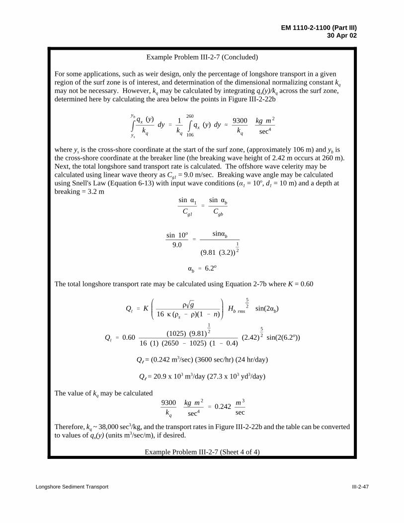
EM 1110-2-1100 (Part III)30 Apr 02
Longshore Sediment Transport III-2-47
myb
ys
qx (y)kq
dy '1kq m
260
106
qx (y) dy . 9300kq
kg m 2
sec4
sin α1
Cg1
'sin αb
Cgb
sin 10o
9.0'
sinαb
(9.81 (3.2))12
αb ' 6.2o
QR ' K ρ g16 κ (ρs & ρ)(1 & n)
Hb rms
52 sin(2αb)
QR ' 0.60 (1025) (9.81)12
16 (1) (2650 & 1025) (1 & 0.4)(2.42)
52 sin(2(6.2o))
9300kq
kg m 2
sec4' 0.242 m 3
sec
Example Problem III-2-7 (Concluded)
For some applications, such as weir design, only the percentage of longshore transport in a givenregion of the surf zone is of interest, and determination of the dimensional normalizing constant kqmay not be necessary. However, kq may be calculated by integrating qx(y)/kq across the surf zone,determined here by calculating the area below the points in Figure III-2-22b
where ys is the cross-shore coordinate at the start of the surf zone, (approximately 106 m) and yb isthe cross-shore coordinate at the breaker line (the breaking wave height of 2.42 m occurs at 260 m). Next, the total longshore sand transport rate is calculated. The offshore wave celerity may becalculated using linear wave theory as Cg1 = 9.0 m/sec. Breaking wave angle may be calculatedusing Snell's Law (Equation 6-13) with input wave conditions (α1 = 10o, d1 = 10 m) and a depth atbreaking = 3.2 m
The total longshore transport rate may be calculated using Equation 2-7b where K = 0.60
QR = (0.242 m3/sec) (3600 sec/hr) (24 hr/day)
QR = 20.9 x 10³ m3/day (27.3 x 10³ yd3/day)
The value of kq may be calculated
Therefore, kq ~ 38,000 sec3/kg, and the transport rates in Figure III-2-22b and the table can be convertedto values of qx(y) (units m3/sec/m), if desired.
Example Problem III-2-7 (Sheet 4 of 4)

EM 1110-2-1100 (Part III)30 Apr 02
III-2-48 Longshore Sediment Transport
volume is called a source. Alternately, any process that results in a net loss of sediment from a controlvolume is considered a sink. Some processes can function as sources and sinks for the same control volume(e.g., longshore sediment transport). The balance of sediment between losses and gains is reflected inlocalized erosion and deposition. In general, longshore movement of sediment into a coastal compartment,onshore transport of sediment, additions from fluvial transport, and dune/bluff/cliff erosion provide the majorsources of sediment. Longshore movement of sediment out of a coastal compartment, offshore transport ofsediment, and aeolian transport and washover that increase beach/island elevation produce losses from acontrol volume. Sediment budgets, including the types and importance of sources and sinks, are discussedin detail in Part IV-5.
(b) The appropriate level of detail for a littoral budget is a function of the intended uses of the littoralbudget, and the available resources to complete the project. The essential components of a littoral budgetinclude a site description, background, and examination of previous analyses. Past and present conditions,and the results of other studies, must be examined before initiating a new budget analysis.
(c) The longshore sediment transport rate must be determined next. This requires data on waveconditions over as long a time period as possible. These waves are propagated to and transformed in the surfzone. Appropriate sediment transport equations must be applied, ideally using historical shoreline positionsand wave conditions for the same time period to, in effect, “calibrate” the transport equations for the studysite. Very often, shoreline change models, which use the sediment transport equations, are applied. Boundaryconditions defined at the start of the analysis are changed, so that sensitivity of the budget to these conditionsmay be evaluated.
(d) The actual sediment budget may then be determined. Usually there are poorly quantified componentsremaining in the analysis, such as offshore gains and losses. These must be estimated using any availabledata, engineering judgment, and the requirement that the budget close. Although a significant effort goes intothe development of a littoral budget, it must be remembered that it is an estimate and may easily be in error.In addition, the budget is usually calibrated with shoreline positions over a number of years, and thereforeindicates long-term average rates of change. It may not be indicative of the changes in any one year.
(2) Variations in longshore sediment transport along the coast.
(a) As described in the next section, noncohesive shorelines are not typically straight. The shorelineorientation and the degree to which waves refract, shoal, and converge or diverge along the shorelinedetermine variations in the potential transport rate along the coast. These variations are importantdeterminants to shoreline change along the coast. For a nonuniform coastline, the potential longshoresediment transport rate is computed at discrete points along the coastline using values of the local breakingwave height and angle, where the latter is expressed relative to the local shoreline orientation. A ray-tracingor grid-based wave refraction analysis is typically employed to determine these values.
(b) Shoreline change may be related to the computed gradients in transport rate along the coast. Forexample, areas of convergent transport may correspond to a sediment sink (or deposition). Areas of divergenttransport may correspond to a sediment source (or erosion if the area is not a source). As long as there is anunlimited sediment source, a shoreline's response to longshore sediment transport should be dependent ongradients in transport along the coast rather than magnitudes of transport.

EM 1110-2-1100 (Part III)30 Apr 02
Longshore Sediment Transport III-2-49
h. Three-dimensionality of shoreline features.
(1) The three-dimensionality of noncohesive shoreline shape and its corresponding underwaterexpression are important to various aspects of engineering design. Dunes are more susceptible tobreakthrough where the beach width fronting the dune is narrow due to the diminished protection affordedby the berm. Noncohesive shorelines are typically neither straight nor of smooth curvature. They often haveisolated “bumps” or more regularly spaced shoreline features. Migration of such shoreline features canundercut or flank the landward ends of coastal structures such as seawalls or groins. For this reason anyregularly spaced (rhythmic) topographic features inherent in the beach/shoreline structure as reflected in itsplanform shape may be of importance to the engineer for consideration of risk factors in evaluation ofprojects. Little is known about these features from a quantitative standpoint, although considerablequalitative descriptions of the features are documented.
(2) Typically, shoreline rhythmic features are classified by their planform (longshore) spacing orapproximate wavelength if they are of reasonably regular form and hence are often referred to as “sandwaves” by many authors. The term “sand wave” in this context should not be confused with underwater sandwaves that are ubiquitous in most marine environments. Planform amplitude or height of the shorelinefeatures (defined as cross-shore distance from embayment to cusp point) often is correlated with thewavelength. That is, longer shoreline planform wavelength (or alongshore spacing) suggests larger planformamplitudes (Sonu 1969). Along most shorelines, a spectrum of rhythmic shapes and sizes is present, makingthe underlying shoreline planform characteristics somewhat confusing. Due to the continuous range of scalein observed shoreline rhythmic features it is impossible to completely separate discussion of the variousfeatures by size since the physics governing the various length scales may be similar.
(3) At the small end of the scale of rhythmic shoreline features (and consequently of lesser engineeringsignificance) are “beach cusps.” Figure III-2-23 is an example of a beach with developed beach cusps.Russell and McIntire (1965) compile observational statistics on beach cusps from a number of ocean beachesand show cusp planform wavelengths (or longshore spacing) from 6 to 67 m. Numerous authors havepostulated theories for the conditions of formation as well as spacing and amplitude of these smaller-scalefeatures.
(4) At present, though, an explanation that would encompass all the numerous small-scale rhythmicfeatures noted along the shoreline is lacking. Extended discussion on these smaller-scale shoreline featurescan be found in Komar (1976).
(5) As an example of larger-scale rhythmic topography, Figure III-2-24 shows a shoreline from TokaiBeach, Japan (Mogi 1960), in which two predominant wavelength scales of rhythmic sinuous topographydominate over a 3-month period of study. The shorter planform wavelengths in this example are on the orderof 250 m while the longer planform wavelengths are on the order of 2.5 km. Although phasing changes areevident, the rhythmic feature length scales appear to have prevailed throughout the different survey periods.Lippmann and Holman (1990) have documented the conditions for rhythmic bars along one section of theNorth Carolina shoreline (Duck, NC). They found that rhythmic bars were a predominant feature observedin 68 percent of video imaging records and noted that during the strongest wave activity the rhythmic featureswere destroyed but that the features returned 5-16 days following peak wave events.
(6) Along beaches in Japan, Hom-ma and Sonu (1963) observed that under certain conditions crescenticbars with a regular alongshore spacing would weld to the shoreline with consequent large cusps formed atthe attachment points (see Figure III-2-25). Sonu (1973) notes a second type of rhythmic topography inwhich rhythmic shoreline features are associated with the presence of rip current cell circulation (see Fig-ure III-2-26). Sonu (1973) noted that both types of rhythmic topography could be present independently
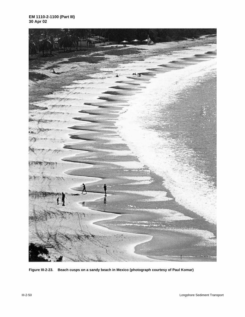
EM 1110-2-1100 (Part III)30 Apr 02
III-2-50 Longshore Sediment Transport
Figure III-2-23. Beach cusps on a sandy beach in Mexico (photograph courtesy of Paul Komar)

EM 1110-2-1100 (Part III)30 Apr 02
Longshore Sediment Transport III-2-51
Figure III-2-24. Shoreline fluctuations in plan view at Tokai Beach, Japan (after Mogi (1960))
Table III-2-3List of Authors Postulating Theories for Cusp Development
Johnson (1910, 1919) Dalrymple and Lanan (1976)
Dolan and Ferm (1968) Dubois (1978)
Escher (1937) Shepard (1973)
Longuet-Higgins and Parkin (1962) Dolan, Vincent, and Hayden (1974)
Russell and McIntire (1965) Flemming (1964)
Bagnold (1940) Krumbein (1944b)
Williams (1973) Komar (1973)
Kuenen (1948) Zenkovitch (1964)
Sonu (1972, 1973) Otvos (1964)
Sonu and Russell (1967) Sonu, McCloy, and McArthur (1967)
Bowen (1973) Bowen and Inman (1969)
Guza and Bowen (1981) Guza and Inman (1975)
Sallanger (1979) Seymour and Aubrey (1985)
Holman and Bowen (1979, 1982) Darbyshire (1977)
Darbyshire and Pritchard (1978) Dean and Maurmeyer (1980)
along a shoreline, and that the crescentic bar type of feature is typically at larger scales than the featuresassociated with rip current cell circulation.
(7) Sonu (1973) details numerous examples of world coastlines with rhythmic shoreline/nearshorefeatures, and notes the ubiquitous nature of these features via their existence on long uninterrupted coastlinesas well as embayment shorelines between headlands, in tideless seas as well as coasts with tidal ranges upto 4 m, and on beaches with grain size ranging from sand to gravel. Observations of the planform wavelength(or alongshore spacing) of the features varies markedly, including 100 to 300 m along the east coast of Florida(Bruun and Manohar 1963); 64 to 218 m between transverse bars on the low-energy sheltered coast

EM 1110-2-1100 (Part III)30 Apr 02
III-2-52 Longshore Sediment Transport
Figure III-2-25. Rhythmic shoreline features associated with the presence of crescenticbars welded to the shoreline
Figure III-2-26. Cusp rhythmic features in conjunction with rip currents underwave action approaching shoreline obliquely (adapted from Sonu (1973))

EM 1110-2-1100 (Part III)30 Apr 02
Longshore Sediment Transport III-2-53
of St. James Island, Florida (Niedoroda and Tanner 1970); 100 to several thousand meters in the case ofthe example shown in Figure III-2-25 (Sonu 1973); up to 1,500 m for giant cusps noted along variousbeaches (Shepard 1952, 1973); and on the order of hundreds of meters along the Atlantic bluff shorelineof Cape Cod, Massachusetts (Aubrey 1980). Sonu and Russell (1967) noted, and later Dolan (1971)measured shoreline rhythmic features along the North Carolina coast with alongshore spacing ranging from150 to 1,000 m with the predominant spacing about 500 to 600 m. In the same study, Dolan (1971) measureplanform amplitudes from 15 to 25 m with large sand waves reaching amplitudes of 40 m. Numerous, well-documented surveys of sand wave/giant cusp rhythmic beach planforms also exist along the Danish andDutch coasts (van Bendegom 1949, Brunn 1954, Verhagen 1989).
(8) Migration rates of rhythmic features vary widely with some studies reporting short-term fluctuationsin position but no net long-term migration. Van Bendegom (1949) documents the monitoring over an 80-yearperiod of large sand waves with amplitudes up to 200 m along the Dutch coast, and discusses thecorresponding cycle of beach erosion and accretion as these waves migrate along the coastline with anaverage speed of 200 m/year. Dolan (1971) noted migration velocities of large sand waves along the NorthCarolina coast ranging from 100 to 200 m/month during heavy weather seasons. Verhagen (1989) hasdocumented sand waves along the Dutch coast with amplitudes from 25 to 2,500 m and longshore speedsranging from 45 to 310 m/year. Sonu (1969) has suggested that migration velocities of such shorelinefeatures are inversely proportional to some power of the feature's alongshore spacing (i.e., the larger thefeature, the slower the movement).
(9) Edge waves and rip currents are often cited as the main contributing forcing functions to theformation of rhythmic topography at various scales. A discussion of edge wave generation and hypothesizedeffects on beaches can be found in Guza and Inman (1975), Huntley and Bowen (1973, 1975a, 1975b, 1979),Huntley (1976), Holman and Bowen (1979, 1982), Wright et al. (1979), Guza and Bowen (1981), and Bowenand Inman (1971). A discussion of rip current formation and its effects on beaches can be found in Bowen(1969), Bowen and Inman (1969), Hino (1974), Dalrymple (1975), Dalrymple and Lanan (1976), Dolan(1971), Komar (1971), Komar and Rea (1976), and Komar (1978). Conclusive evidence proving themechanisms for the formation of the many types of rhythmic topography is lacking.
(10) From an engineering standpoint the importance of rhythmic shoreline features (especially largerones) and their potential for migration should not be overlooked in planning engineering structures or inanalysis of design dune width for storm protection. For example, van Bendegom (1949) documents thestructural failure of a groin due to the erosion produced by a large, migrating sand wave along the Dutchcoast. Brunn (1954) described migrating sand waves along the Danish North Sea coast with observedplanform spacings on the order of 300 to 2,000 m and amplitudes on the order of 60 to 80 m in areas whereseasonal beach change was only 20 m/year and long-term shoreline recession only 2 m/year. In this regard,Brunn (1954) also cites a case of a sand wave of 900 m wavelength and 60 m amplitude with a migrationspeed of 700 m/year, and notes the difficulty of drawing definitive conclusions on average shorelinemovements in such areas. Dolan (1971) noted that the regular spacing of dune breaching on Bodie Island,North Carolina, during the Ash Wednesday storm of 7 March 1962 correlated well with the rhythmictopography seen in the shoreline. Dolan (1971) also documented erosion along the Cape Hatteras, NorthCarolina, shoreline corresponding to embayments of rhythmic topography and suggested that when analyzingbeach variability for specific sites, in addition to the seasonal recession-progradation cycle, additionalvariation (about 20 percent along the Outer Banks) should be considered to account for migration of therhythmic topographic features.
(11) In practice, aerial photography at a reasonable scale (1 in. = 100 m or larger) or shoreline surveysare necessary to document the existence of rhythmic shoreline features. Sets of such aerialphotographs/shoreline surveys with common control points and interspersed over long periods of time should

EM 1110-2-1100 (Part III)30 Apr 02
III-2-54 Longshore Sediment Transport
RRo
' Co % C1βθ
% C2βθ
2
(III-2-24)
be useful in detailing both the potential existence and characteristics of such features for consideration inengineering planning.
i. Empirical shoreline models.
(1) In nature, many sections of coastline which are situated in the lee of a natural or artificial headlandfeature a curved shoreline geometry. Where sections of coastline are situated between two headlands, andparticularly when there is a single, dominant wave direction, the shoreline may likewise assume a curved or“scalloped” shape (see Figure III-2-27a). In both cases, the curved portion of the shoreline related to theheadland(s) is termed a crenulate or “spiral bay.” Because of their geometries, these shorelines are alsosometimes termed “parabolic,” “zeta-bay,” or “log-spiral” shorelines. The shape results from longshoretransport processes which move sediment in the downdrift direction along the down-wave section of theshoreline, and from processes associated with wave diffraction which move sediment in the opposite directionin the immediate lee of the up-wave headland.
(2) Krumbein (1944b) and Yasso (1965) were among the first investigators to suggest that many“static” shorelines in the vicinity of rocky or erosion-resistant headlands could be fit to a log-spiral curve.Silvester (1970); Silvester and Ho (1972); Silvester, Tsuchiya, and Shibano (1980); and Hsu and Evans(1989) utilized the concept to develop empirical guidance for maximum coastal indentation between twoheadlands or coastal structures (such as seawalls or breakwaters) based on one dominant wave direction.Practical application of the approach requires identification of a predominant wave direction and the properorigin of the log-spiral curve. In a more theoretical effort, LeBlond (1972, 1979) derived equations for anequilibrium shoreline shape in the shadow zone of an upcoast headland based upon many simplifyingassumptions concerning refraction and diffraction and found the resulting shoreline to be very similar to thelog spiral shape. Rea and Komar (1975), Parker and Quigley (1980), and Finkelstein (1982) have also notedthe similarity of bay shoreline shapes to log spiral curves. Walton (1977) and Walton and Chiu (1977)demonstrated that the log spiral curve is robust in the sense that most smooth curves found in nature can befit to a log spiral if fortuitous values of its parameters are chosen. Walton (1977) presents a simplifiedprocedure for evaluating a dynamic progression of static equilibrium shorelines downcoast from headland-type features using the concept of the littoral energy rose.
(3) Using shoreline data from prototype bays considered to be in static equilibrium and from physicalmodels, Hsu, Silvester, and Xia (1987, 1989a, 1989b) presented an alternate expression to approximate theshoreline in the lee of headland-type features:
where the geometric parameters R, Ro, β, and θ are as shown in Figure III-2-27a, and values for thecoefficients C0, C1, and C2 are shown in Figure III-2-27b. The distance Ro corresponds to a control line drawnbetween the ends of the headlands that define a given section of shoreline. In the case of a single, upcoastheadland, the distance Ro is the length of a control line drawn from the end of the headland to the nearest pointon the downcoast shoreline at which the shoreline is parallel with the predominant wave crest. The distanceR, measured from the end of the upcoast headland, defines the location of the shoreline at angles θ measuredfrom the predominant wave crest. The angle β is that between the predominant wave direction and the controlline Ro.
(4) The tidal shoreline which Equation 2-24 represents is not clear, but might be interpreted to representthe mean water shoreline. The data upon which Equation 2-24 is based are principally limited to β > 22E.

EM 1110-2-1100 (Part III)30 Apr 02
Longshore Sediment Transport III-2-55
Figure III-2-27. Spiral bay geometry: (a) definition sketch and (b) coefficients describingparabolic shoreline shape (Silvester and Hsu 1993)

EM 1110-2-1100 (Part III)30 Apr 02
III-2-56 Longshore Sediment Transport
Figure III-2-28. Elemental volume on equilibrium beach profile
Additionally, Equation 2-24 is intended for application for β # θ # 180E, and assumes that a predominantwave direction exists at the site of interest. The latter is often not the case in nature, and so engineeringjudgement must be utilized in practical application of this method. For θ > 180E, the distance R may beassumed to be constant and equal to the value of R computed at θ = 180E.
(5) Additional empirical guidance on shoreline change at seawalls is provided in Walton andSensabaugh (1979) where additional localized recession at a seawall under a storm condition (hurricaneEloise along the Florida panhandle), is provided. Similar guidance for other storms and other locations is notavailable, although McDougal, Sturtevant, and Komar (1987) and Komar and McDougal (1988), havereported similar findings at laboratory scales.
(6) The approach(es) outlined above may be useful for rough, preliminary calculations and estimatesof “static” shoreline equilibriums when the assumptions necessary for application of the approaches arefulfilled, where detailed dynamics of the changing shoreline are not sought, and where time and/or budgetconstraints preclude a more detailed approach. For detailed prediction of shoreline change due to longshoregradients in sand transport or otherwise complicated geometries, a preferred approach would be to utilize aphysical model and/or a numerical model, as appropriate to the scale of the study area.
j. Analytical longshore sand transport shoreline change models.
(1) If the angle of the shoreline is small with respect to the x axis and simple relationships describe thewaves, analytical solutions for shoreline change may be developed. As an example, utilizing the expressionprovided in Equation 2-7b for longshore sediment transport along with the assumption that the breaking waveangle αb is small, the following planform shoreline change equation can be derived utilizing the coordinatesystem given in Figures III-2-28 and III-2-29:

EM 1110-2-1100 (Part III)30 Apr 02
Longshore Sediment Transport III-2-57
Figure III-2-29. Definition of local breaker angle
ε M2 yMx 2
'MyM t (III-2-25)
ε 'K H 2
b Cgb
8ρ
ρs & ρ1
1 & n1
dB % dc(III-2-26)
where
and where dB = beach berm height above still-water level; dc = depth of appreciable sand transport asmeasured from still-water level. Equation 2-25 is a partial differential equation, as it is dependent on bothspace (variable x) and time (variable t). A number of researchers have employed this equation or slight varia-tions of it to provide analytical solutions to shoreline change under certain assumptions (the boundary con-ditions and initial conditions of the problem). Pelnard-Considére (1956) first presented an analytical solutionto this simplified shoreline change equation for the case of an impermeable groin or jetty impounding thelongshore sand transport on the updrift side of the structure under a stationary (constant) wave climate.Pelnard-Considére also verified its applicability with laboratory experiments and derived analytical solutionsof the linearized shoreline change equation for two other boundary conditions: shoreline evolution updriftof an impermeable groin (with bypassing) and release of an instantaneous plane source of sand on the beach.

EM 1110-2-1100 (Part III)30 Apr 02
III-2-58 Longshore Sediment Transport
EXAMPLE PROBLEM III-2-8
FIND:Compute the shoreline geometry of a crenulate bay located between two rock headlands for a
shoreline where one dominant wave direction exists.
GIVEN:The distance between the ends of the headlands is 175 m. The incident wave crests make an angle
of 30 deg with a line drawn between the two headlands.
SOLUTION:
From Figure III-2-27b, the values of the coefficients for the wave angle β = 30 deg areapproximately C0 = 0.05, C1 = 1.14, and C2 = -0.19. The location of the shoreline may be predictedby plotting the distance R, measured from the end of the upwave headland, at angles θ measured fromthe line drawn between the headlands. The values R/Ro for various arbitrary angles between the waveangle, 30 deg, and a maximum angle, 180 deg, are computed from Equation 2-24. The correspondingdimensional values of R are then computed by multiplying R/Ro by the distance between the headlandsRo = 175 m. Representative examples are given below:
For θ = 30 deg: R = [ 0.05 + 1.14(30/30) - 0.19(30/30)2 ] ( 175 m ) = 175 m
For θ = 75 deg: R = [ 0.05 + 1.14(30/75) - 0.19(30/75)2 ] ( 175 m ) = 83 m
For θ = 180 deg: R = [ 0.05 + 1.14(30/180) - 0.19(30/180)2 ] ( 175 m ) = 41 m
For θ > 180E, the distance R may be assumed to be constant and equal to the value of R computed atθ = 180E.
(2) Le Méhauté and Brebner (1961) discuss solutions for shoreline change at groins, with and withoutbypassing of sand, and the effect of sudden dumping of material at a given point. They also present solutionsfor the decay of an undulating shoreline, and the equilibrium shape of the shoreline between two headlands.
(3) Bakker and Edelman (1965) modified the longshore sand transport rate equation to allow for ananalytical treatment without linearization. The sand transport rate is divided into two different cases:

EM 1110-2-1100 (Part III)30 Apr 02
Longshore Sediment Transport III-2-59
QR ' Qo Ka tan (αb ) for 0 # tan αb # 1.23 (III-2-27a)
QR ' QoKb
tan (αb )for 1.23 < tan (αb) (III-2-27b)
and
where Ka and Kb are constants. The growth of river deltas was studied with these equations.
(4) Bakker (1968) extended a one-line shoreline change theory to include the shoreline and an additionaloffshore depth contour to describe beach planform change. Bakker hypothesized that the two-line theoryprovides a better description of sand movement downdrift of a long groin since it describes representativechanges in the contours seaward of the groin head. Near structures such as groins, offshore contours mayhave a different shape from the shoreline. The two lines in the model are represented by a system of twodifferential equations which are coupled through a term describing cross-shore transport. According toBakker (1968), the cross-shore transport rate depends on the steepness of the beach profile; a steep profileimplies offshore sand transport; and a gently sloping profile implies onshore sand transport. Additionalcomplex solutions of cases with groins under very simplistic assumptions are discussed in Bakker, Klein-Breteler, and Roos (1971). Le Méhauté and Soldate (1977) provide an analytical solution of the linearizedshoreline change equation for the spread of a rectangular beach fill. Walton (1994) has extended this caseto the fill case with tapered ends.
(5) Walton and Chiu (1979) present two derivations of the linearized shoreline change equation. Thedifference between the two approaches, which both arrive at the same partial differential equation, is that oneuses the so-called “CERC Formula” (see Equation 2-5) for describing the longshore sand transport rate bywave action and the other a formula derived by Dean (1973) based on the assumption that the major sandtransport occurs as suspended load. Walton and Chiu (1979) also present solutions for beach fill in atriangular shape, a rectangular gap in a beach, and a semi-infinite rectangular fill, and present previousanalytical solutions in the literature in a nondimensionalized graphical solution form.
(6) Dean (1984) gives a brief survey of some analytical shoreline change solutions applicable to beachnourishment calculations, especially in the form of characteristic quantities describing loss percentages. Onesolution describes the shoreline change between two groins initially filled with sand. Larson, Hanson, andKraus (1987) provide a review of a number of analytical solutions to the one-line model as well as additionalsolutions where the amplitude of the longshore sand transport rate is a discontinuous function of x, theshoreline coordinate in the longshore direction.
(7) Analytical solutions presented here are in the nondimensionalized form of Walton and Chiu (1979)and easily adaptable to solving simple scenarios. More difficult scenarios are best handled by a numericalmodel. In arriving at all solutions, it is tacitly assumed that sand is always available for transport unlessexplicitly restricted by boundary and/or initial conditions.
(8) The first case to be considered is that of a structure trapping sediment. This formulation can beapplied to the prediction of the shoreline updrift and downdrift of a littoral barrier extending perpendicularto the initially straight and uniform shoreline. At the barrier, all sediment is assumed to be trapped by thebarrier (no bypassing). This boundary condition requires that the shoreline at the structure be parallel to theincoming wave crests. Figure III-2-30 shows the resulting shoreline evolution with increasing time updrift(accretion) and downdrift (erosion). Figures III-2-31a, III-2-31b, and III-2-31c are nondimensionalizedsolution graphs (at different scales) for the condition of no sand transport at the structure location (x = 0),

EM 1110-2-1100 (Part III)30 Apr 02
III-2-60 Longshore Sediment Transport
Figure III-2-30. Structure placed perpendicular to shore
erf ( ) '2π m
( )
0e &z 2
dz
with the boundary condition at the structure being tan αb = dy/dx, and the boundary condition at x = 4 beingy = 0 for all times. The initial condition for this solution is that y = 0 for t = 0. This particular solution graphcan be utilized to estimate planform shapes on the updrift side of coastal structures where bypassing does nottake place.
(9) The dimensionalized solution for these conditions is given by Pelnard-Considére (1956) to be
(III-2-28)y ' 2 ε t tan(αb)1π
exp &x
2 ε t
2
&x
2 ε terfc x
2 ε t, for t < tf
where tf is the time at which the structure fills to its capacity via this solution and where erfc( ) is thecomplementary error function defined as erfc( ) = 1 - erf( ) where erf( ) is the error function and
Both erfc ( ) and erf ( ) are tabulated in various mathematical handbooks. Figures III-2-32 and III-2-33provide graphs of erfc ( ) and erf ( ).
(10) The time required for the structure to fill to capacity t = tf can be found from the previous solutionwith ordinate x = 0; i.e.,

EM 1110-2-1100 (Part III)30 Apr 02
Longshore Sediment Transport III-2-61
Figure III-2-31. Nondimensionalized solution graphs (at different scales)for the condition of no sand transport at the structure location
0.6
0.5
.D 0.4 ~ c .3
>- ~ 0 .3
0.2
0 .1
0 .5 1.5 2 .5
X
z...JET (a)
0.06
0 .05
0 .04
0.03
0.02
0.01
1.5 2 .5
_ x_ z...JET
0 .00 1
0 .0008
.0 ~ c 0. 0006 0
>-~ N 0.0004
0 .0002
0 2 2 .2 2.4 2. 6 2.8
X
2...JET (c)

EM 1110-2-1100 (Part III)30 Apr 02
III-2-62 Longshore Sediment Transport
Figure III-2-32. Error function
Figure III-2-33. Complementary error function
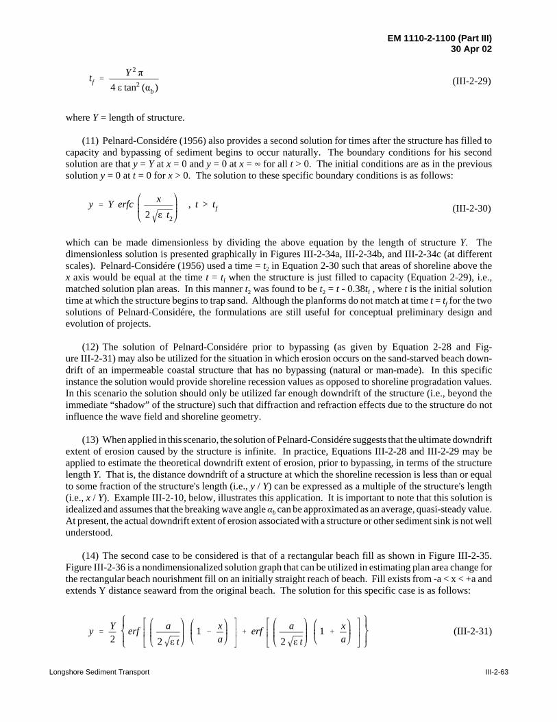
EM 1110-2-1100 (Part III)30 Apr 02
Longshore Sediment Transport III-2-63
tf 'Y 2 π
4 ε tan2 (αb ) (III-2-29)
y ' Y erfc x2 ε t2
, t > tf (III-2-30)
where Y = length of structure.
(11) Pelnard-Considére (1956) also provides a second solution for times after the structure has filled tocapacity and bypassing of sediment begins to occur naturally. The boundary conditions for his secondsolution are that y = Y at x = 0 and y = 0 at x = 4 for all t > 0. The initial conditions are as in the previoussolution y = 0 at t = 0 for x > 0. The solution to these specific boundary conditions is as follows:
which can be made dimensionless by dividing the above equation by the length of structure Y. Thedimensionless solution is presented graphically in Figures III-2-34a, III-2-34b, and III-2-34c (at differentscales). Pelnard-Considére (1956) used a time = t2 in Equation 2-30 such that areas of shoreline above thex axis would be equal at the time t = tf when the structure is just filled to capacity (Equation 2-29), i.e.,matched solution plan areas. In this manner t2 was found to be t2 = t - 0.38tf , where t is the initial solutiontime at which the structure begins to trap sand. Although the planforms do not match at time t = tf for the twosolutions of Pelnard-Considére, the formulations are still useful for conceptual preliminary design andevolution of projects.
(12) The solution of Pelnard-Considére prior to bypassing (as given by Equation 2-28 and Fig-ure III-2-31) may also be utilized for the situation in which erosion occurs on the sand-starved beach down-drift of an impermeable coastal structure that has no bypassing (natural or man-made). In this specificinstance the solution would provide shoreline recession values as opposed to shoreline progradation values.In this scenario the solution should only be utilized far enough downdrift of the structure (i.e., beyond theimmediate “shadow” of the structure) such that diffraction and refraction effects due to the structure do notinfluence the wave field and shoreline geometry.
(13) When applied in this scenario, the solution of Pelnard-Considére suggests that the ultimate downdriftextent of erosion caused by the structure is infinite. In practice, Equations III-2-28 and III-2-29 may beapplied to estimate the theoretical downdrift extent of erosion, prior to bypassing, in terms of the structurelength Y. That is, the distance downdrift of a structure at which the shoreline recession is less than or equalto some fraction of the structure's length (i.e., y / Y) can be expressed as a multiple of the structure's length(i.e., x / Y). Example III-2-10, below, illustrates this application. It is important to note that this solution isidealized and assumes that the breaking wave angle αb can be approximated as an average, quasi-steady value.At present, the actual downdrift extent of erosion associated with a structure or other sediment sink is not wellunderstood.
(14) The second case to be considered is that of a rectangular beach fill as shown in Figure III-2-35.Figure III-2-36 is a nondimensionalized solution graph that can be utilized in estimating plan area change forthe rectangular beach nourishment fill on an initially straight reach of beach. Fill exists from -a < x < +a andextends Y distance seaward from the original beach. The solution for this specific case is as follows:
(III-2-31)y 'Y2
erf a2 ε t
1 &xa
% erf a2 ε t
1 %xa

EM 1110-2-1100 (Part III)30 Apr 02
III-2-64 Longshore Sediment Transport
Figure III-2-34. Nondimensional solution curve for plan view of sedimentaccumulation at a coastal structure after natural bypassing initiated
0.8
~ 0.6 >,
0.4
0.2
0 0 0.5 1.5 2 2.5
X
2vEt
(a)
0.18
0.16
0.14
0.12
>- 0.1 '-..._ >,
0.08
0.06
0.04
0.02
0 1.0 1.2 1.4 1.6 1.8 2 2.2 2.4
__ x_
2.Vct
(b)
.005
.004
.003
~ >,
.002
.001
0 2 2.1 2.2 2.3 2.4 2.5
X
2vEt
(c)
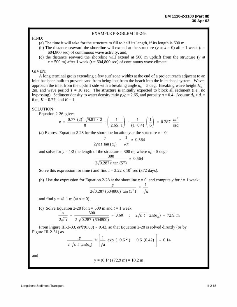
EM 1110-2-1100 (Part III)30 Apr 02
Longshore Sediment Transport III-2-65
ε '0.77 (2)2 9.81 @ 2
8@ 1
2.65&1@ 1
(1&0.4)16
' 0.287 m 2
sec
y2 ε t tan (αb)
'1π
– 0.564
3002 0.287 t tan (50 )
– 0.564
y2 0.287 (604800) tan (50 )
'1π
x2 ε t
'500
2 0.287 (604800)' 0.60 ; 2 ε t tan(αb ) ' 72.9 m
y2 ε t tan(αb)
– 1π
exp (&0.6 2 ) & 0.6 (0.42) ' 0.14
EXAMPLE PROBLEM III-2-9FIND:
(a) The time it will take for the structure to fill to half its length, if its length is 600 m.(b) The distance seaward the shoreline will extend at the structure (y at x = 0) after 1 week (t =
604,800 sec) of continuous wave activity, and;(c) the distance seaward the shoreline will extend at 500 m updrift from the structure (y at
x = 500 m) after 1 week (t = 604,800 sec) of continuous wave climate.
GIVEN:A long terminal groin extending a few surf zone widths at the end of a project reach adjacent to an
inlet has been built to prevent sand from being lost from the beach into the inlet shoal system. Wavesapproach the inlet from the updrift side with a breaking angle αb = 5 deg. Breaking wave height Hb =2m, and wave period T = 10 sec. The structure is initially expected to block all sediment (i.e., nobypassing). Sediment density to water density ratio ρs/ρ = 2.65, and porosity n = 0.4. Assume dB + dc =6 m, K = 0.77, and K = 1.
SOLUTION:Equation 2-26 gives
(a) Express Equation 2-28 for the shoreline location y at the structure x = 0:
and solve for y = 1/2 the length of the structure = 300 m, where αb = 5 deg:
Solve this expression for time t and find t = 3.22 x 10⁷ sec (372 days).
(b) Use the expression for Equation 2-28 at the shoreline x = 0, and compute y for t = 1 week:
and find y = 41.1 m (at x = 0).
(c) Solve Equation 2-28 for x = 500 m and t = 1 week.
From Figure III-2-33, erfc(0.60) • 0.42, so that Equation 2-28 is solved directly (or byFigure III-2-31) as
andy = (0.14) (72.9 m) = 10.2 m

EM 1110-2-1100 (Part III)30 Apr 02
III-2-66 Longshore Sediment Transport
yY
' [ exp(&u 2) & π u erfc (u) ]
u 'x
2 ε tf
'xY
1π
tan(αb )
xY
' u πtan(αb )
' 0.96 πtan(50 )
' 19.4
EXAMPLE PROBLEM III-2-10
FIND:
The distance downdrift of a structure at which the shoreline recession is less than or equal to10 percent of the structure's length before sand begins to naturally bypass the structure.
GIVEN:
A long groin extending a few surf zone widths has been built with no artificial sand fill oneither side. The groin's length, measured from the original shoreline, is Y. Assume that the waveactivity is continuous with breaking angle αb = 5 deg.
SOLUTION:
The structure becomes filled to capacity at time tf. Substitution of Equation 2-29 for tf intoEquation 2-28 yields:
where
Determine the value u (graphically or by iteration), for which y/Y = 0.10. Find u – 0.96. Determine the downdrift distance x (relative to the structure's length Y) using this value for u andusing αb = 5 deg:
That is, the shoreline recession is equal to or less than 10 percent of the structure's length beyondapproximately 19.4 structure-lengths downdrift. If, for instance, the structure's length was Y =200 m, the downdrift location at which the shoreline recession is less than 20 m (at the time thestructure is filled to capacity) is (19.4)(200) = 3,880 m downdrift of the structure.
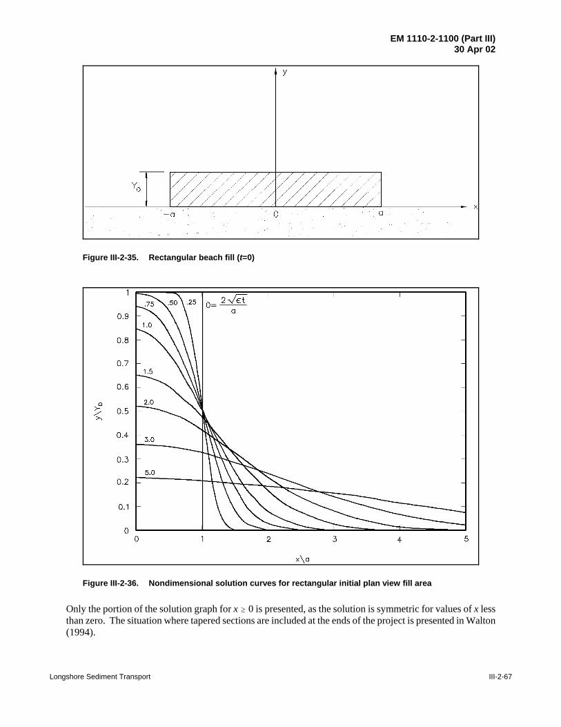
EM 1110-2-1100 (Part III)30 Apr 02
Longshore Sediment Transport III-2-67
Figure III-2-35. Rectangular beach fill (t=0)
Figure III-2-36. Nondimensional solution curves for rectangular initial plan view fill area
Only the portion of the solution graph for x $ 0 is presented, as the solution is symmetric for values of x lessthan zero. The situation where tapered sections are included at the ends of the project is presented in Walton(1994).

EM 1110-2-1100 (Part III)30 Apr 02
III-2-68 Longshore Sediment Transport
p(t) '1π
ε ta
exp &aε t
2
& 1 % erf aε t
(III-2-32)
Figure III-2-37. Proportion of fill p(t) remaining within limits of rectangular plan view fill area
(15) This equation may be integrated over the project limits to allow estimation of the proportion p(t) offill left within the project boundaries at a given time after project initiation to give:
which is plotted in Figure III-2-37 as a function of the inverse of the nondimensionalized beach half lengthparameter a
2 ε t
(16) A third case to be considered is that of a triangular beach fill as shown in Figure III-2-38. Atriangular planform beach nourishment might exist at a location where either a truck dumping of sand occursor where drag scraping of sand from the offshore occurs. The solution for this specific case (where theoriginal fill has been assumed triangular in shape) is:
(III-2-33)y '
Yo
2(1&X) erf (U(1&X)) % (1%X) erf (U (1%X)) &2 Xerf (UX)
%1πU
(e &U 2 (1%X)2% e &U 2 (1&X)2
& 2e &(UX)2)

EM 1110-2-1100 (Part III)30 Apr 02
Longshore Sediment Transport III-2-69
Figure III-2-38. Triangular beach fill (t=0)
X 'xa
and U 'a
2 ε t
y 'Yo
21 % erf x
2 ε t(III-2-35)
where
(17) Figure III-2-39 is a nondimensionalized solution graph for the case of a triangular planform beachnourishment. Only the portion of the solution graph for x $ 0 is presented, as the solution is symmetric forvalues of x less than zero.
(18) A fourth case to be considered is that of a long fill project with a gap as shown in Figure III-2-40.For the case in which a beach nourishment has been placed on an existing beach but a gap has been left inthe beach nourishment project (such as occurred in a beach nourishment project on Jupiter Island, Florida,in 1974), the following solution would apply:
(III-2-34)y 'Y2
erfc a2 ε t
1 &xa
% erfc a2 ε t
1 %xa
The nondimensionalized solution graph for this particular planform of beach nourishment is provided inFigure III-2-41. Only the portion of the solution graph for x $ 0 is presented, as the solution is symmetricfor values of x less than 0.
(19) A fifth case to be considered is that of the end of a rectangular fill on a long beach nourishmentproject as shown in Figure III-2-42. The nondimensional solution graph for the case of a semi-infinite beachfill where the fill is contained within the area x > 0 is given in Figure III-2-43. This semi-infinite beach fillcase can be utilized to provide the shape of the end of a long beach fill and the extent of the fill as itprogresses down the coast with time. The solution for this specific case is

EM 1110-2-1100 (Part III)30 Apr 02
III-2-70 Longshore Sediment Transport
ε '0.77 (3)2 9.81 @ 3
81
2.65 & 11
1 & 0.41
3 % 7
– 0.47 m 2/s
a2 ε t
'2,500
2 0.47 (259,200)' 3.58
xa
' 1.0 yYo
' 0.56 hence, y ' 0.56 (50) ' 28 m
a2 ε t
'2,500
2 0.47 (7,257,600)' 0.68
xa
' 1.0 yY0
' 0.46 hence, y ' 0.46 (50) ' 23 m
EXAMPLE PROBLEM III-2-11
FIND:The width of the beach at the ends of the fill after 3 days and after 12 weeks of design wave action
on the beach fill.
GIVEN:A beach nourishment 5,000 m in length is placed on a reasonably stable shoreline to widen the beach
as a protective measure for upland construction during storms. The new beach width is to be 50 m andis to be placed at the same berm elevation as the natural beach dB = 3 m. Depth of appreciable sandtransport as estimated from historical profiles in the region is assumed dc = 7 m. A design wave for thearea is estimated to be Hb = 3 m, T = 12 sec, αb = 10 deg. The sediment size of the natural beach is thesame size as the fill sediment size and ratio of sediment density to water density (i.e., specific gravity)is 2.65. The porosity of beach is n = 0.4. The K factor is assumed = 0.77, and κ is assumed = 1.
SOLUTION:a = 5,000/2 = 2,500 m ; YO = 50 m
At fill ends x/a = 1.0
From Equation 2-26
After 3 days (t = 259,200 sec)
From Figure III-2-36, for
After 12 weeks (t = 7,257,600 sec)
From Figure III-2-36, for

EM 1110-2-1100 (Part III)30 Apr 02
Longshore Sediment Transport III-2-71
Figure III-2-39. Nondimensional solution curves for triangular initial plan view fill area
Figure III-2-40. Long fill project with a gap (t=0)

EM 1110-2-1100 (Part III)30 Apr 02
III-2-72 Longshore Sediment Transport
Figure III-2-41. Nondimensional solution curve for long fill with gap in plan viewfill area
Figure III-2-42. Semi-infinite beach fill (t=0)
y ' Yo 1 % erf x2 ε t
(III-2-36)
(20) For the situation in which the fill is in area x < 0, the graph can be utilized by flipping the solutionpresented around the y axis.
(21) A sixth case to be considered is the nourishment fill initially placed in the area (x > 0) andmaintained at the initial beach width Y within the project area. The solution for the planform beach adjacentto the fill (x # 0) is given by

EM 1110-2-1100 (Part III)30 Apr 02
Longshore Sediment Transport III-2-73
Figure III-2-43. Nondimensional solution curve for semi-infinite plan view fill area
y ' Yo erfc x2 ε t
(III-2-37)
y ' w & R 1 &xR
tan (αb ) %2 tan(αb )
R j4
n'0
2R(2n % 1)π
2
exp &ε (2n % 1)2π2t4R2
cos (2n % 1)πx2R
(III-2-38)
(22) For the analogous case to the above instance where the planform fill is placed in the area (x < 0) andmaintained at the initial beach width Y in the project area, the solution (for x $ 0) is:
where the nondimensionalized solution graph has the same nondimensionalized solution as provided earlierin Figure III-2-34.
(23) A final case is presented for the situation in which groins and fill are implemented together as in Fig-ure III-2-44. Where the initial fill is placed to the end of the groin, the solution is given by Dean (1984) as:
The nondimensionalized shoreline solution graph for this situation is provided in Figure III-2-45 for theparameters W/L = 0.25 and tan (αb) = 0.1.

EM 1110-2-1100 (Part III)30 Apr 02
III-2-74 Longshore Sediment Transport
Figure III-2-45. Nondimensional solution curve for plan view of rectangular fill areabetween coastal structures (w/l = 0.25; tan αb = 0.1)
Figure III-2-44. Beach fill placed with groins (t=0)
(24) Since Equation 2-24 is linear, the above solutions can be combined to address more complexsituations than those presented. As an example, consider the case in which staged construction of a beachnourishment project takes place over a long length of beach and the fill area of the beach is to be confinedin the reach x < 0 and maintained at its fill width. Equation 2-37 could be utilized for solving this particularexample in the case that the entire fill was placed at time t = 0. Instead, consider that the fill is placed in

EM 1110-2-1100 (Part III)30 Apr 02
Longshore Sediment Transport III-2-75
Figure III-2-46. Width of maintained beach (x < 0) as a function of time
stages with the plan view dimension of the fill as a function of time given in Figure III-2-46. For thisparticular scenario, the solution (at time t) analogous to Equation 2-37 only with the planform beach built instaged increments (as per Figure III-2-46) is:
(III-2-39)y ' Yo erfc x2 εt
% Y1&Yo erfc x2 ε (t& t1)
% Y2&Y1 erfc x2 ε (t& t2)
which can be nondimensionalized and solved utilizing the nondimensionalized solution graph provided bythe simpler case of Equation 2-37 given in Figure III-2-34.
(25) It should be recognized that the linearized form of shoreline solution will produce a higher rate ofshoreline change by overestimating the longshore transport rate because 2αb > sin(2αb) in the linearized sandtransport solution. Thus, under properly estimated parameters for idealized conditions, a higher rate ofattenuation of beach fills will be obtained than is expected to occur in reality, thus providing a conservativeanswer to project losses.
(26) As a final point, it is noted that when wave angles are very large and the difference between thewave direction and shoreline orientation exceeds 45 deg, the true form of the shoreline diffusivity constantbased on the nonlinear sin(2α) term in the sand transport equation will be negative, which totally changes thecharacteristics of the shoreline change model equation. In these cases, the shoreline evolves in an unstablemanner equivalent to running the previous stable solution forms backwards through time. In other words,a shoreline having a perturbation placed on it (such as a beach fill) would see a growth of the perturbationtoward an elongated cuspate feature as time progresses rather than seeing the smoothing out of theperturbation as given in solutions of the preceding paragraphs. This type of shoreline instability may possiblyexplain certain shoreline features such as cuspate forelands which are ubiquitous on elongated bays wherethe dominant wave action is along the major axis of the bay and at large angles to the prevailing shorelinetrends (Walton 1972).

EM 1110-2-1100 (Part III)30 Apr 02
III-2-76 Longshore Sediment Transport
ε '0.77 (1)2 9.81 @ 1
81
2.65 & 11
1 & 0.416
– 0.0508 m2
sec
y (1 mile, 3 months)' 50 @ erfc 1,609
2 0.0508 @ 7.78 × 10⁶meters
. 50 @ erfc (1.28)
. 50 (0.07) – 3.5 m
EXAMPLE PROBLEM III-2-12
FIND:
The level of protection (i.e., width of beach) afforded to a historical lighthouse as a consequence ofthe nourishment project at the end of 3, 6, 8, 9, and 12 months after initial fill placement. The lighthouseis situated at the shoreline 1 mile (. 1,609 m) south of the south end of the proposed beach at theinitiation of the project fill.
GIVEN:
A long beach fill is placed along a north-south directed stretch of shoreline along the east coast ofthe United States (i.e., the azimuth of the offshore direction is 90 deg). The project is to be constructedand maintained continuously to design project width throughout the project fill area. The project willbe constructed in two stages; Stage 1 will provide a fill width of 50 m, and Stage 2 (to be placed3 months after initial placement) will add another 50 m of beach width, making the total finished projectwidth = 100 m. Assume that: Hb = 1 m; T = 10 sec; αb = 5 deg (from the north) K is assumed = 0.77,and κ = 1.0. Sediment density to water density ratio (i.e., specific gravity) = ρs/ρ = 2.65; porosity n =0.4; dB + dc = 6 m. Note that except for breaking wave height Hb, these are the same wave and sedimentparameters as given in Example III-2-8.
SOLUTION:
For Hb = 1 m, with other parameters the same as the previous problem;
At the end of the first 3 months, the solution of Equation 2-37 (graphical solution provided by Figure III-2-34) can be utilized with t = 3 months . 7.78 × 10⁶ sec, and x = 1 mile . 1,609 m:
(Continued)

EM 1110-2-1100 (Part III)30 Apr 02
Longshore Sediment Transport III-2-77
y(x, t) ' Yo @ erfc x2 ε t
% (Y1 & Yo) @ erfc x2 ε (t & t1)
y(x, t) ' 50 @ erfc x2 ε t
% 50 erfc x2 ε t
@ 1
1&t1
t
' term 1 % term 2
x2 ε t
Example Problem III-2-12 (Concluded)
For times beyond the 3-month initial fill placement and maintenance, a solution of the form ofEquation 2-39 must be utilized. In this particular case, the solution would be of the form (where Yo= 50 m, Y1 - Yo = 50 m, and t1 = 3 months):
which can be reformulated to be:
The solution is provided in the table below:
(1)
t
(2) (3)
(2) @ 1&t1
t
&1/2(4)
erfc((2))
(5)
erfc((3))
(6)
term 1
(7)
term 2
(8)
y
6 mo.= 15.8 × 10⁶ sec.
0.90 0.90 (1.414)= 1.27
0.20 0.07 10.0 3.5 13.5 m
9 mo.= 23.7 × 10⁶ sec.
0.73 0.73 (1.225)= 0.89
0.30 0.21 15.0 10.5 25.5 m
12 mo.= 31.6 × 10⁶ sec.
0.63 0.63 (1.155)= 0.73
0.37 0.30 18.5 15.0 33.5 m
Note that the solution form assumes that the fill is constantly maintained at its design width. Thiswould probably not be achievable in practice, and solutions would have to be modified in accordwith good engineering judgment.

EM 1110-2-1100 (Part III)30 Apr 02
III-2-78 Longshore Sediment Transport
III-2-4. Numerical Longshore Sand Transport Beach Change Models
As opposed to analytical solutions of shoreline change, which simplify the equations used to predict beachevolution, mathematical modeling facilitates generalization of these equations so that input parameters mayvary in time and in the longshore, and possibly cross-shore, dimensions. Also, numerical models becomenecessary where difficult boundary conditions are encountered (say at groins or offshore breakwaters)because of shoreline morphology or wave transformation. Numerical models of beach change perform bestwhen a perturbation is introduced to a system that is in equilibrium. The perturbation to the system mightbe an introduction or removal of littoral material (e.g., beach fill, sand mining, release of sediment due to aflooded river or landslide) or placement of a hardened structure (e.g., groins, detached breakwaters, seawalls,revetments). Historical trends of beach change and knowledge of the littoral budget are typically used tocalibrate and verify the controlling equations, then forecasts may be simulated as a function of variousengineering alternatives and/or wave climate scenarios. Therefore, beach response as a function of complexcoastal processes may be readily examined in detail with mathematical models. However, the limitationsinherent in the controlling equations, and assumptions implied in developing “representative” parametersrequire that model results be carefully interpreted, ideally within the context of other coastal engineeringanalyses.
a. Types of longshore transport models
(1) Fully three-dimensional models.
(a) In nature, nearshore beach change due to waves, circulation patterns, and longshore currents varieswith time and location; therefore, equations to fully describe effects of these processes on beach evolutionmust be three-dimensional and time-dependent. Development of these equations is still an area of activeresearch, and fully three-dimensional models are not available for routine engineering design.
(b) The intent of three-dimensional models is to describe bottom elevation changes which may vary inthe cross-shore and longshore directions. These models provide insight into wave transformations andcirculation for complicated bathymetry and in the vicinity of nearshore structures. However, they are lessuseful for making long-term shoreline evolution calculations because they are computationally intensive.These models also involve poorly known empirical coefficients such as those related to bottom friction,turbulent mixing, and sediment transport. Integrating the calculated local distributions of sediment transportover the cross-shore and for long time periods may lead to erroneous results because small local inaccuracieswill be amplified over a long simulation. Because of their intent to predict local process parameters (e.g.,waves, currents, sediment transport), they require a detailed data set for calibration, verification, andsensitivity testing, perhaps from a companion physical model study or field data collection.
(2) Schematic three-dimensional models. Schematic three-dimensional models simplify the controllingequations of fully three-dimensional models by, for example, restricting the shape of the profile or calculatingglobal rather than point transport rates. Bakker (1968) has developed a two-line model which allows theevolution of two contours to be independently simulated. From this model, Perlin and Dean (1983)developed an n-line model that allows an arbitrary number of contour lines to represent the beach profile.Most schematic multi-line models developed to date are restricted to monotomic profile representations. Formodels that represent the profile by more than one contour, it is necessary to specify a relationship for cross-shore sediment transport. Schematic three-dimensional models have not yet reached the stage of wideapplication due to their complexity, requirement for considerable computational resources, and need forexpertise in operational applications.

EM 1110-2-1100 (Part III)30 Apr 02
Longshore Sediment Transport III-2-79
∆y∆ t
%1
dB % dC
∆QR
∆x± q ' 0 (III-2-40)
αb ' αbg & αsg ' αbg & tan&1 dydx
(III-2-41)
(3) One-line (two-dimensional) models.
(a) The Large Scale Sediment Processes Committee at the Nearshore Processes Workshop in St.Petersburg in 1989 concluded that long-term simulations of beach change are more reasonably formulatedon the basis of total or bulk transport models such as Equation 2-7. These models have fewer coefficientsthan three-dimensional models and provide no details of the sediment transport profile. However, they maybe calibrated and verified to include the integrated effect of all of the local processes on the total transport.
(b) The shoreline change models developed from bulk transport models are often referred to as one-linemodels. One-line models assume that the beach profile is a constant shape; thus, the controlling equationsmay be solved for one contour line only (usually taken as the shoreline). Many shoreline change models havebeen developed and applied (e.g., Komar 1973a; LeMéhauté and Soldate 1977; Walton, Liu, and Hands 1988;and many others). Documented nonproprietary, one-line models that are also presently available include amodel developed at the University of Florida (Dean and Grant 1989, Dean and Yoo 1992, 1994), and thecomputer model GENESIS (GENEralized model for SImulating Shoreline change) (Hanson 1987; Hansonand Kraus 1989; Gravens, Kraus, and Hanson 1991).
(c) One-line models used to estimate longshore sand transport rates and long-term shoreline changesgenerally assume that the profile is displaced parallel to itself in the cross-shore direction. The profile mayinclude bars and other features but is assumed to always maintain the same shape. This assumption is bestsatisfied if the profile is in equilibrium. The one-line model is formulated on the conservation equation ofsediment in a control volume or shoreline reach, and a bulk longshore sand transport equation. It is assumedthat there is an offshore closure depth dC at which there are no significant changes in the profile, and the upperend of the active profile is at the berm crest elevation dB. The constant profile shape moves in the cross-shoredirection between these two limits. This implies that sediment transport is uniformly distributed over theactive portion of the profile. The incremental volume of sediment in a reach is simply (dB + dC)∆x∆y, where∆x is the reach of shoreline segment, and ∆y is the cross-shore displacement of the profile. Conservation ofsediment volume may be written as
in which QR is the longshore transport rate, q is a line source or sink of sediment along the reach, and t is time(Figure III-2-28). As examples, line sources of sediment may be rivers and coastal cliffs, and sinks may beproduced by sand mining or dredging.
(d) The longshore transport rate is evaluated using equations similar to Equation 2-7. These requiremeasurement or calculation of the breaking wave angle relative to the beach. The local wave angle relativeto the beach is the difference between the wave angle relative to a model baseline and the shoreline anglerelative to the model baseline (Figure III-2-29),
where x is the distance alongshore, and y is the distance offshore.
(e) If the angle of the shoreline is small with respect to the x axis and simple relationships describe thewaves, analytical solutions for shoreline change may be developed, as discussed in the previous section. For

EM 1110-2-1100 (Part III)30 Apr 02
III-2-80 Longshore Sediment Transport
QR ' H 2b sig Cgb a1 sin2αb & a2 cosαb
dHb sig
dx(III-2-42)
a1 'K1
16ρs
ρ& 1 (1 & n) (1.416)
52
(III-2-43)
a2 'K2
8ρs
ρ& 1 (1 & n) m (1.416)
72
(III-2-44)
more complex conditions, such as time-varying wave conditions, large shoreline angles, variable longshorewave height (perhaps due to diffraction), multiple structures, etc., numerical models can be used in manyinstances.
b. Shoreline Change Model GENESIS.
(1) Overview.
(a) The numerical model GENESIS (Hanson 1987; Hanson and Kraus 1989; Gravens, Kraus, andHanson 1991) is an example of a one-line shoreline change model that is supported for use both on personalcomputer and mainframe systems (see Cialone et al. (1992)) and has a companion system of support programs(Gravens 1992). GENESIS has been applied to numerous coastal engineering projects, and it calculatesshoreline change due to spatial and temporal differences in longshore transport as produced by breakingwaves. GENESIS is used in conjunction with grid-based wave transformation models that develop valuesof breaking wave height and angle for various representative wave periods and approach azimuths along thecoast. Shoreline change at grid cells along the coastline is computed in the time domain as a function of thesecomputed values of the breaking wave height and angle.
(b) As discussed by Hanson (1987) and Hanson and Kraus (1989), the empirical predictive formula forthe longshore sand transport rate used in GENESIS is
The nondimensional parameters a1 and a2 are given by
and
where K1 and K2 are empirical coefficients, treated as calibration parameters, and m is the average bottomslope from the shoreline to the depth of active longshore sand transport. The factors involving 1.416 are usedto convert the K1 and K2 coefficients from use with rms wave height to use with significant wave height(which is the statistical wave height required by GENESIS). That is, Equation 2-43 is presented such thatK1 is equivalent to Krms (as opposed to Ksig) in Equation 2-7. Nonetheless, both longshore sand transportcoefficients K1 and K2 should be viewed as calibration parameters that are to be adjusted to match measuredpositions of shoreline change (Hanson and Kraus 1989).
(c) The first term in Equation 2-42 corresponds to Equation 2-7, and accounts for longshore sandtransport produced by obliquely incident breaking waves. The second term in Equation 2-42 is used todescribe the effect of another generating mechanism for longshore sand transport, the longshore gradient inbreaking wave height. The contribution arising from the longshore gradient in wave height is usually much

EM 1110-2-1100 (Part III)30 Apr 02
Longshore Sediment Transport III-2-81
smaller than that from oblique wave incidence in an open-coast situation. However, in the vicinity ofstructures, where diffraction produces a substantial change in breaking wave height over a considerable lengthof beach, inclusion of the second term provides an improved modeling result, accounting for diffractioneffects.
(d) The boundary conditions at the ends of a study area in a shoreline change modeling project mustbe specified. There are three common boundary conditions: no sand transport (QR = 0), free sand transport(dQR/dx = 0), and partial sand transport (QR … 0). The locations of the study area ends should be selected withthese options in mind. Large headlands or jetties which completely block the longshore transport are goodchoices for model boundaries. At these locations QR = 0. Points where the position of the shoreline has notchanged for many years are also good locations for boundaries. At these points, the gradient in longshoretransport is small so that a free transport condition can be specified (dQR/dx = 0). At some locations, thelongshore transport rate is known and can be used as a boundary condition (i.e., artificial sand bypassing ata jetty). If none of these “good” locations exist, engineering judgment must be used.
(e) In all cases, results should be calibrated and verified using known shoreline positions and waveconditions for the longest period possible. The modeler also attempts to use wave data applicable to theperiod between the dates of the calibration shorelines. The GENESIS technical reference (Hanson and Kraus1989) discusses in full the operation of shoreline change numerical simulation models.
(2) Input data requirements and model output.
(a) As discussed by Gravens (1991, 1992), preparation and analysis of the input and output data filesoccupy a substantial portion, perhaps the majority, of the time spent on a detailed shoreline change modelingproject. Gravens (1991, 1992) stresses that the data gathering organization and analysis process cannot beoveremphasized because (1) it forms the first necessary level in understanding coastal processes at the projectsite, and (2) the simulation results must be interpreted within the context of regional and local coastalprocesses, and the natural variability of the coastal system. Success in modeling shoreline change depends,to a large extent, on preparation and analysis of the input data.
(b) General input information required by GENESIS includes the spatial and temporal ranges of thesimulation, structure and beach fill configurations (if any), values of model calibration parameters, andsimulated times when output is desired. Initial and measured (if available) shoreline positions as referencedto a baseline established for the simulation are also required. Offshore and nearshore (if available) waveinformation and associated reference depths are used to calculate longshore sand transport rates. Outputinformation produced by GENESIS includes intermediate and final calculated shoreline positions, and netand gross longshore sand transport rates.
(3) Capabilities and limitations.
(a) GENESIS was designed to predict long-term trends of the beach plan shape in its evolution fromone given initial condition. This change is usually caused by a notable perturbation; for example, by beachfill placement, sand mining, sand discharge from a river, construction of a detached breakwater, or jettiesconstructed at a harbor or inlet. In engineering applications and tests of GENESIS, modeled shoreline reacheshave ranged from about 2 to 35 km with a grid resolution of 15 to 90 m, and simulation periods have spannedfrom approximately 6 months to 20 years, with wave data typically entered at simulated time intervals in therange of 30 min to 6 hr (Gravens, Kraus, and Hanson 1991).
(b) Hanson and Kraus (1989) and Gravens, Kraus, and Hanson (1991) discuss the capabilities andlimitations of GENESIS. The model allows an almost arbitrary number and combination of groins, jetties,

EM 1110-2-1100 (Part III)30 Apr 02
III-2-82 Longshore Sediment Transport
detached breakwaters, beach fills, and seawalls, with a primary limitation in this regard being the size andspeed of the computer and the maximum number of grid cells that can be accommodated by the program.Compound structures (such as T-shaped, Y-shaped, and spur groins) may be simulated with varying degreesof realism. At least five grid cells are required to reasonably model the shoreline behind and betweenstructures. Sand bypassing around and transmission through groins and jetties may be simulated, as well asdiffraction at detached breakwaters, jetties, and groins. Transmission through detached breakwaters may besimulated. GENESIS allows multiple wave trains to be input (such as from independent wave sources), andthe wave information may include arbitrary values of wave height, period, and direction. As presented inEquation 2-42, sand transport is calculated due to oblique wave incidence and a longshore gradient in waveheight.
(c) GENESIS is not applicable to simulating a randomly fluctuating beach system in which no trendin evolution of the shoreline is evident. In particular, GENESIS is not applicable to calculating shorelinechange in the following situations which involve beach change that is not related to coastal structures,boundary conditions, or spatial differences in wave-induced longshore sand transport: beach change insideinlets or in areas dominated by tidal flow; beach change produced by wind-generated currents; storm-inducedbeach erosion in which cross-shore sediment transport processes are dominant; and scour at structures.GENESIS also does not include wave reflection from structures; cannot reliably simulate tombolo or salientdevelopment at a detached breakwater; and there is no direct provision for changing tide level. In addition,the basic assumptions in the development of shoreline change modeling theory apply.
(4) Example application - Bolsa Chica, California.
(a) As discussed by Hanson and Kraus (1989) and Gravens (1990b), GENESIS (either its predecessor,Version 1, or the current Version 2) has been applied at numerous project sites, including locations in Alaska(Chu et al. 1987); California (Gravens 1990a); Louisiana (Hanson, Kraus, and Nakashima 1989; Gravens1994); New Jersey (Gravens, Scheffner, and Hubertz 1989); New York (Cialone et al. 1994); Florida (by theU.S. Army Engineers District, Jacksonville); and outside the United States (Hanson and Kraus 1986;Kraus 1988). Application of the model to assess a proposed structured inlet system at Bolsa Chica,California, is summarized below (Gravens 1990a) to illustrate model use in coastal project evaluation andrefinement.
(b) GENESIS was applied to an approximately 10-mile-long shoreline reach from Anaheim Bay to theSanta Ana River, California (Figure III-2-47) as part of a comprehensive multi-tasked engineeringinvestigation for the California State Lands Commission (SLC). The shoreline change modeling effort wasdirected towards quantifying the potential long-term impacts of the proposed entrance on adjacent shorelines,and to investigate mitigation of any adverse impacts induced by the entrance. Three major components wereinvolved in the shoreline modeling effort: (1) a preliminary shoreline response study, in which availablewave and shoreline data were used to provide preliminary estimates of the introduction of a littoral barrierin the local littoral cell; (2) a comprehensive wave hindcast of locally generated wind sea and North Pacificswell conditions from 1956 to 1975 at 3-hr intervals, and an 18-month hindcast of South Pacific swell; and(3) comprehensive shoreline response modeling using the hindcast wave data to predict response of theproject area to various design alternatives. Discussion herein is focussed on this third component, includingpreparation of input data sets and analysis of model output, as they pertain to application of GENESIS. Fora more complete description of the project, the reader is directed to Gravens (1990a).

EM 1110-2-1100 (Part III)30 Apr 02
Longshore Sediment Transport III-2-83
Figure III-2-47. Bolsa Chica, California, study area (Gravens 1990a)
(c) The modeled reach from Anaheim Bay to the Santa Ana River forms a littoral cell, including acomplete barrier to littoral transport at Anaheim Bay, and a submarine canyon offshore of Newport Beach(Figure III-2-47). Coastal structures and features of importance within the model reach include the eastAnaheim jetty, the sea cliffs at Huntington Beach, the Huntington Beach pier, and the north jetty at the mouthof the Santa Ana River. Each of these features influences the evolution of adjacent shoreline and wasrepresented in the shoreline change model. The sea cliffs at Huntington Beach serve to pin the shorelinebetween the cliffs and Anaheim Bay to the northwest and the Santa Ana River to the southeast. TheHuntington Pier and the east Anaheim Bay jetty modify the local breaking wave pattern and produce a localshoreline signature unique to these structures. Beaches between Anaheim Bay and the Santa Ana River haveaccreted an average of 1.3 m/year (4.4 ft/year) between 1934 and 1983.
(d) Ten shoreline position data sets dating from 1878 and 1983 were analyzed to determine historicaland representative shoreline change trends. As a result of this analysis, the 1963, 1970, and 1983 shorelineswere determined to be representative, and were summarized at 61-m (200-ft) intervals for model calibration(1963 to 1970) and verification (1970 to 1983).
(e) For the comprehensive shoreline response study, hindcast wave estimates at stations located nearthe lateral boundaries of the modeled shoreline reach were transformed from the hindcast stations to theoffshore boundary of the GENESIS grid using the linear wave propagation model RCPWAVE (RegionalCoastal Processes Wave Model; Ebersole 1985; Ebersole, Cialone, and Prater 1986) (Figure III-2-48). Useof two hindcast stations allowed systematic variations in the incident waves (alongshore wave height andangle) to be accounted for in RCPWAVE and ultimately in GENESIS.
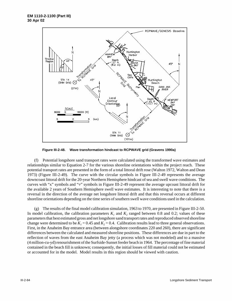
EM 1110-2-1100 (Part III)30 Apr 02
III-2-84 Longshore Sediment Transport
Figure III-2-48. Wave transformation hindcast to RCPWAVE grid (Gravens 1990a)
(f) Potential longshore sand transport rates were calculated using the transformed wave estimates andrelationships similar to Equation 2-7 for the various shoreline orientations within the project reach. Thesepotential transport rates are presented in the form of a total littoral drift rose (Walton 1972, Walton and Dean1973) (Figure III-2-49). The curve with the circular symbols in Figure III-2-49 represents the averagedowncoast littoral drift for the 20-year Northern Hemisphere hindcast of sea and swell wave conditions. Thecurves with “x” symbols and “«” symbols in Figure III-2-49 represent the average upcoast littoral drift forthe available 2 years of Southern Hemisphere swell wave estimates. It is interesting to note that there is areversal in the direction of the average net longshore littoral drift and that this reversal occurs at differentshoreline orientations depending on the time series of southern swell wave conditions used in the calculation.
(g) The results of the final model calibration simulation, 1963 to 1970, are presented in Figure III-2-50.In model calibration, the calibration parameters K1 and K2 ranged between 0.8 and 0.2; values of theseparameters that best estimated gross and net longshore sand transport rates and reproduced observed shorelinechange were determined to be K1 = 0.45 and K2 = 0.4. Calibration results lead to three general observations.First, in the Anaheim Bay entrance area (between alongshore coordinates 220 and 260), there are significantdifferences between the calculated and measured shoreline positions. These differences are due in part to thereflection of waves from the east Anaheim Bay jetty (a process which was not modeled) and to a massive(4 million-cu-yd) renourishment of the Surfside-Sunset feeder beach in 1964. The percentage of fine materialcontained in the beach fill is unknown; consequently, the initial losses of fill material could not be estimatedor accounted for in the model. Model results in this region should be viewed with caution.
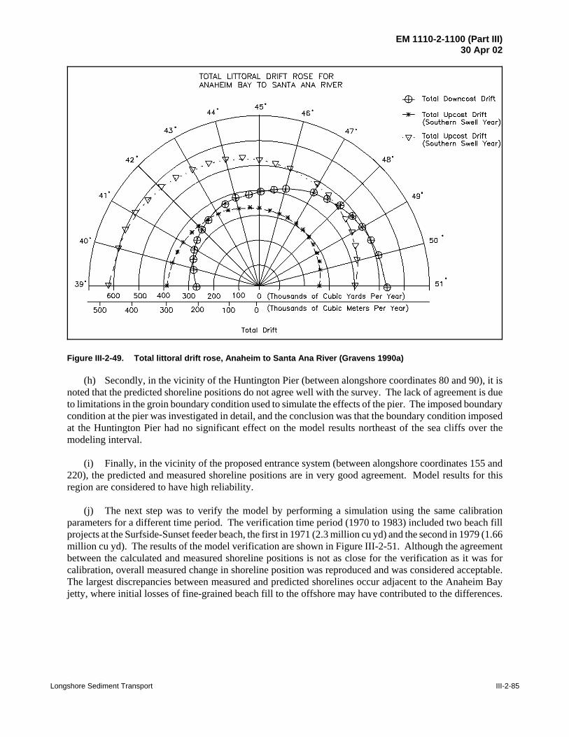
EM 1110-2-1100 (Part III)30 Apr 02
Longshore Sediment Transport III-2-85
Figure III-2-49. Total littoral drift rose, Anaheim to Santa Ana River (Gravens 1990a)
(h) Secondly, in the vicinity of the Huntington Pier (between alongshore coordinates 80 and 90), it isnoted that the predicted shoreline positions do not agree well with the survey. The lack of agreement is dueto limitations in the groin boundary condition used to simulate the effects of the pier. The imposed boundarycondition at the pier was investigated in detail, and the conclusion was that the boundary condition imposedat the Huntington Pier had no significant effect on the model results northeast of the sea cliffs over themodeling interval.
(i) Finally, in the vicinity of the proposed entrance system (between alongshore coordinates 155 and220), the predicted and measured shoreline positions are in very good agreement. Model results for thisregion are considered to have high reliability.
(j) The next step was to verify the model by performing a simulation using the same calibrationparameters for a different time period. The verification time period (1970 to 1983) included two beach fillprojects at the Surfside-Sunset feeder beach, the first in 1971 (2.3 million cu yd) and the second in 1979 (1.66million cu yd). The results of the model verification are shown in Figure III-2-51. Although the agreementbetween the calculated and measured shoreline positions is not as close for the verification as it was forcalibration, overall measured change in shoreline position was reproduced and was considered acceptable.The largest discrepancies between measured and predicted shorelines occur adjacent to the Anaheim Bayjetty, where initial losses of fine-grained beach fill to the offshore may have contributed to the differences.

EM 1110-2-1100 (Part III)
30 Apr 02
III-2-86Longshore Sedim
ent Transport
Figure III-2-50. Model calibration results, Bolsa Chica (Gravens 1990a)
g BOLSA CHICA: MODEL CALIBRATION
;= HUNTING1tlN PIER
~3000 1 --~-~~~~ :. ~ ' 000000~-0000000-~00000~ ~ Pocific Coast Hwy a
1000 ••••• -~···~-····· ·············~---············ -··--····· ~
!5 ·-~. ~ .... '·=· ' ... ~ .. ' ... : .. ~ .... ;:~-· ~ 0 Z ~ ~ ~ ~ ~ ~ ~ B ~ ~ ~ ~ 4800~ AI..DNGSHORE COORDINATE (cell spacing = 200 ft)
4400
4000
t3600 .83200 E ,g2800 a;
;:
HlJNT't4GTON PER
?" ~···-··--·~ ..•... -············· SEA CUFFS
.r/ .. ~·· .. ··· ~1100
!~
/,11' .--~~-···-··-·
/~// Pacirc Coast Hoy ... ···· .··
100=1 / •...•. ••·••·
~~r/ ...... / ... .... .... ··•··
-- 1963 (Jun) surveyed shoreline -·- 1970 (Ap~ surveyed shorel"ne ........ 1970 (Ap~ predicted shonll'ne
0 J··;- ;~"~,j':"''~n;',""";' 11 1 1 I i 1 c a : e 1 ; 1 U ; 1 I : I : 1 I I : I J : I I I 1 I I I I 1 : I I I 1 I : I I j I I I I Ji1 ":'-','
11 ~~·~
100 ~ ~ 160 180 220 ~ ~ zo 0 z 40 eo BO
ALONGSHORE COORDINATE (ceU spacing = 200 ft)

EM 1110-2-1100 (Part III)
30 Apr 02
Longshore Sediment Transport
III-2-87
Figure III-2-51. Model verification results, Bolsa Chica (Gravens 1990a)
g BOLSA CHICA: MODEL VERifiCATION ;: HUNTING11lN PER
~~-- ~ ~ ~ ~ m ~ ~ * s 200 220 240 210
4100
44GO
4000
13100 .83200
!2800 s ~:MOO
~2000 ~1&00 ~GOO
800
~
ALONGSHORE COORDINATE (ceU spacing = 200 ft)
HUNTINGTON PER
~ '··-.~-~
--1970 (Ap~ surveyed shoreliw -·- 1983 4Jan) surveyed shoreine -------- 1983 (Jan) predicted shoreline
Beach FiR 6:u )d) 1971: 2;300/XX) 1979: \644/XX)
~ .. ~ .. ; .. ··"' ·· .... A ... ··· PacifiC eoast Hwy ····--·-.... .J" ... ·········· '·· ........... _ ~ ...... · ·-······-............. .
· ....... ··················· ·····-~·· ..... - SANTA AAA RIVER JETTY ~I v ... t I I ,. ....... __ ,""
0 I··, I I I I I I I I i I I I I I I I I I I I I I I I I I I I I I •• I I I I 0 I I I I I I I u I • I I I I I I ' I I • I I I • I ; I I I
220 240 260 '100 120 ~ 110 110 200 0 ~ ~ 10 10 ALONGSHClRE CCIORilW.TE (cel!lpCICitg = 200 ft)

EM 1110-2-1100 (Part III)30 Apr 02
III-2-88 Longshore Sediment Transport
(k) After model calibration and verification, eight conceptual design alternatives were modeled, andseveral simulation variations were performed for each alternative. The intent of the simulations was toquantify the shoreline impacts of the proposed Bolsa Chica navigable ocean entrance system. In thesimulation of Alternatives 1 and 3, no beach fill was included along the modeled reach. For Alternatives 2,4, 5, 6, and 8, renourishment of the Surfside-Sunset feeder beach was specified at 1 million cu yd every 5years. Alternatives 7 and 8 modeled impact mitigation sand management techniques. The 1983 shorelinewas used as the initial shoreline, and all model tests were performed for 5- and 10-year simulation (prediction)periods using a randomly selected 10-year time history of Northern Hemisphere sea and swell conditions.The Southern Hemisphere swell component of the incident wave climate was varied from alternatingavailable southern swell wave conditions, low-intensity southern swell, and high-intensity southern swell topredict a range of influence.
(l) Model results and analysis from 24 production simulations are documented by Gravens (1990a);only results from one alternative are presented here for illustrative purposes. Predicted changes in 10-yearpost-project shoreline position with Alternative 8 are shown in Figure III-2-52. Alternative 8 includes twoshore-perpendicular jetties spaced 245 m apart and extending approximately 425 m offshore, a detachedbreakwater composed of three sections located offshore of the entrance channel, a feeder beach at Surfside-Sunset, and impact mitigation sand management. The impacts of this entrance system with the specified sandmanagement plan as compared to a without-project 10-year projection are shown in Figure III-2-53. Thisalternative satisfied the criteria established by the SLC for successful impact mitigation. The SLC specifiedthat only sand accumulating within 460 m of the entrance jetties may be used by sand bypassing/backpassing,and that a successful sand management plan would predict more accretive, or equal or less erosive, conditionsthan would occur without the project in place.
(m) Conclusions from shoreline change modeling of Bolsa Chica Bay were as follows:
• The proposed site of the new entrance system is located in a region of converging longshore sandtransport.
• Locating the entrance system approximately 1.6 km up- or downcoast from the proposed site wouldnot significantly change the predicted shoreline response.
• Implementation of a sand management plan would allow for the mitigation of adverse shorelineimpacts.
• The Surfside-Sunset feeder beach nourishment program must be continued in order to maintain theshoreline within 3.2 km of the Anaheim Bay entrance. However, the proposed entrance system wouldneither aggravate nor improve the situation.
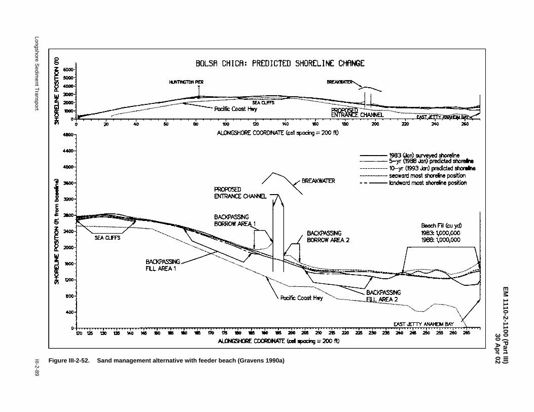
EM 1110-2-1100 (Part III)
30 Apr 02
Longshore Sediment Transport
III-2-89
Figure III-2-52. Sand management alternative with feeder beach (Gravens 1990a)
g
;= i ~lr:7
0
........ --······-····-····-·······
20 40
4100
4400
4000
i: ! 300-.7 ??q·.
;: i:
BOO
400
BOLSA CHICA: PREDICTED SHORELINE CHANGE
HI.INTIGTtlN PER
~--:.~-· ··-·--·-···-· SEA CLFFS
·-·······-~PacifiC Coast Hwy
~ ----~~ ·-·-····-·-.. :::::~··-·--·-····--
60 80 100 120 MO 160 180
Al..DNGSHClRE COORJ)NATE (cell spacing = 200 ft) 200 220 240 260
---1983 4Jan) ~ shorefne -·-·-5-yr (1988 Jon) precfded shorfJne ----------- 10-yr (1993 .bl) precfcted shcnlne ---seaward most shorelne position - - -- landward most shoreline position
Beach Fill (cu ycD 1983: 1,000,000 1988: 1,000,000
EAST JETTY ANAt£JM BAY . o I , .. ., , , , " , " , 1 " " ,. , " 1 " " 1 , " , 1 , " , 1 , , " 1 , , " 1 , , " 1 , a a 'I , " 'I , " , 1 " " 1 , " , 1 " " ,. " , r a " • 1 , " 1 " " ;: " , ,. " , 1 , , " 1 , " 'I " " I' , " 1 • , • • 1 • • "l • • " 1 120z~mM•••••~w••••••3m220maa240a~~-~
AI..ONGSHORE COORDIW"E (t:el tpOCi1g = 200 ft)

EM 1110-2-1100 (Part III)30 Apr 02
III-2-90 Longshore Sediment Transport
Figure III-2-53. Predicted shoreline change from 1983 shoreline position with sand management alternativeand feeder beach (Gravens 1990a)
III-2-3. References
Aubrey 1980Aubrey, D. G. 1980. “Our Dynamic Coastline,” Oceanus, Vol 23, No. 4, pp 4-13.
Bagnold 1940Bagnold, R. A. 1940. “Beach Formation by Waves: Some Model Experiments in a Wave Tank,” JournalInst. Civil Engineering, Vol 15, pp 27-52.
Bagnold 1963Bagnold, R. A. 1963. “Beach and Nearshore Processes; Part I: Mechanics of Marine Sedimentation,” TheSea: Ideas and Observations, Vol 3, M. N. Hill, ed., Interscience, New York, pp 507-528.
Bailard 1981Bailard, J. A. 1981. “An Energetics Total Load Sediment Transport Model for a Plane Sloping Beach,”Journal of Geophysical Research, Vol 86, No. C11, pp 10938-10954.
Bailard 1984Bailard, J. A. 1984. “A Simplified Model for Longshore Sediment Transport,” Proceedings, 19thInternational Coastal Engineering Conference, American Society of Civil Engineers, New York, pp 1454-1470.
Bailard and Inman 1981Bailard, J. A., and Inman, D. L. 1981. “An Energetics Bedload Model for a Plane Sloping Beach: LocalTransport,” Journal of Geophysical Research, Vol 86, pp 2035-2043.

EM 1110-2-1100 (Part III)30 Apr 02
Longshore Sediment Transport III-2-91
Bakker 1968Bakker, W. T. 1968. “The Dynamics of a Coast with a Groin System,” Proceedings of the 11th CoastalEngineering Conference, American Society of Civil Engineers, pp 492-517.
Bakker and Edelman 1965Bakker, W. T., and Edelman, T. 1965. “The Coastline of River Deltas,” Proceedings of the 9th CoastalEngineering Conference, American Society of Civil Engineers, pp 199-218.
Bakker, Klein-Breteler, and Roos 1971Bakker, W. T., Klein-Breteler, E. H. J., and Roos, A. 1971. “The Dynamics of a Coast with a GroinSystem,” Proceedings of the 12th Coastal Engineering Conference, American Society of Civil Engineers,pp 1001-1020.
Beach and Sternberg 1987Beach, R. A., and Sternberg, R. W. 1987. “The Influence of Infragravity Motions on Suspended SedimentTransport in the Inner Surf Zone,” Proceedings of Coastal Sediments '87, American Society of CivilEngineers, pp 913-928.
Bendat and Piersol 1971Bendat, J. S., and Piersol, A. G. 1971. Random Data: Analysis and Measurement Procedures, Wiley-Interscience, New York.
Berek and Dean 1982Berek, E. P., and Dean, R. G. 1982. “Field Investigation of Longshore Transport Distribution,” Proceedings,18th International Conference on Coastal Engineering, American Society of Civil Engineers, pp 1620-1639.
Bodge 1986Bodge, K. R. 1986. “Short-Term Impoundment of Longshore Sediment Transport,” Ph.D. diss., Departmentof Coastal and Oceanographic Engineering, University of Florida, Gainesville.
Bodge 1988Bodge, K. R. 1988. “Longshore Current and Transport Across Non-Singular Equilibrium Beach Profiles,”Proceedings, 21st International Conf. on Coastal Engineering, American Society of Civil Engineers,pp 1396-1410.
Bodge and Dean 1987aBodge, K. R., and Dean, R. G. 1987a. “Short-Term Impoundment of Longshore Transport,” Proceedingsof Coastal Sediments '87, American Society of Civil Engineers, pp 468-483.
Bodge and Dean 1987bBodge, K. R., and Dean, R. G. 1987b. “Short-Term Impoundment of Longshore Sediment Transport,”Miscellaneous Paper CERC-87-7, U.S. Army Engineer Waterways Experiment Station, Vicksburg, MS.
Bodge and Kraus 1991Bodge, K. R., and Kraus, N. C. 1991. “Critical Examination of Longshore Transport Rate Magnitude,”Proceedings, Coastal Sediments '91, American Society of Civil Engineers, pp 139-155.
Bowen 1969Bowen, A. J. 1969. “Rip Currents: 1. Theoretical Investigations,” Journal of Geophysical Research, Vol 74,pp 5467-78.

EM 1110-2-1100 (Part III)30 Apr 02
III-2-92 Longshore Sediment Transport
Bowen 1973Bowen, A. J. 1973. “Edge Waves and the Littoral Environment,” Proceedings 13th Conf. on Coast. Eng.,American Society of Civil Engineers, pp 1313-20.
Bowen and Guza 1978Bowen, A. J., and Guza, R. T. 1978. “Edge Waves and Surf Beat,” Journal Geophysical Research, Vol 83,pp 1913-20.
Bowen and Inman 1966Bowen, A. J., and Inman, D. L. 1966. “Budget of Littoral Sands in the Vicinity of Port Arguello, California,”Technical Memorandum No. 19, Coastal Engineering Research Center, U.S. Army Corps EngineerWaterways Experiment Station, Vicksburg, MS.
Bowen and Inman 1969Bowen, A. J., and Inman, D. L. 1969. “Rip Currents: 2. Laboratory and Field Observations,” Journal ofGeophysical Research, Vol 74, pp 5478-90.
Bowen and Inman 1971Bowen, A. J., and Inman, D. L. 1971. “Edge Waves and Crescentic Bars,” Journal of Geophysical Research,Vol 76, No. 76, pp 8662-71.
Box and Jenkins 1976Box, G. E. P., and Jenkins, G. M. 1976. “Time Series Analysis, Forecasting, and Control,” Holden-Day,San Francisco, CA, p 575.
Brenninkmeyer 1976Brenninkmeyer, B. M. 1976. “In Situ Measurements of Rapidly Fluctuating, High SedimentConcentrations,” Marine Geology, Vol 20, pp 117-128.
Brunn 1954Brunn, P. 1954. “Migrating Sand Waves and Sand Humps, with Special Reference to Investigations Carriedout on the Danish North Sea Coast,” Proceedings 5th Conf. on Coast. Eng., pp 269-95.
Bruno and Gable 1976Bruno, R. O., and Gable, C. G. 1976. “Longshore Transport at a Total Littoral Barrier,” Proceedings of the15th International Conference on Coastal Engineering, American Society of Civil Engineers, pp 1203-1222.
Bruno, Dean and Gable 1980Bruno, R. O., Dean, R. G., and Gable, C. G. 1980. “Littoral Transport Evaluations at a DetachedBreakwater,” Proceedings of the 17th International Conference on Coastal Engineering, American Societyof Civil Engineers, pp 1453-1475.
Bruno, Dean, Gable, and Walton 1981Bruno, R. O., Dean, R. G., Gable, C. G., and Walton, T. L. 1981. “Longshore Sand Transport Study atChannel Island Harbor, California,” Technical Paper No. 81-2, Coastal Engineering Research Center,U.S. Army Engineer Waterways Experiment Station, Vicksburg, MS.
Bruun and Manohar 1963Bruun, P., and Manohar, M. 1963. “Coastal Protection for Florida,” Florida Engineering and IndustrialExperiment Station Bulletin No. 113, University of Florida, Gainesville.

EM 1110-2-1100 (Part III)30 Apr 02
Longshore Sediment Transport III-2-93
Caldwell 1956Caldwell, J. M. 1956. “Wave Action and Sand Movement Near Anaheim Bay, California,” U.S. Army Corpsof Engineers, Beach Erosion Board, Technical Memorandum No. 68.
Chu, Gravens, Smith, Gorman and Chen 1987Chu, Y., Gravens, M. B., Smith, J. M., Gorman, L. T., and Chen, H. S. 1987. “Beach Erosion Control Study,Homer Spit, Alaska,” Miscellaneous Paper CERC-87-15, U.S. Army Engineer Waterways ExperimentStation, Vicksburg, MS.
Cialone et al. 1992Cialone, M. A., Mark, D. J., Chou, L. W., Leenknecht, D. A., Davis, J. E., Lillycrop, L. S., and Jensen, R. E.1992. “Coastal Modeling System (CMS) User's Manual,” Instruction Report CERC-91-1, U.S. ArmyEngineer Waterways Experiment Station, Vicksburg, MS.
Cialone, Neilans, Carson, and Smith (in preparation)Cialone, M. A., Neilans, P. J., Carson, F. C., and Smith, J. M. “Long-term Shoreline Response Modeling atWesthampton Beach, New York,” in preparation, U.S. Army Engineer Waterways Experiment Station,Vicksburg, MS.
Coakley and Skafel 1982Coakley, J. P., and Skafel, M. G. 1982. “Suspended Sediment Discharge on a Non-Tidal Coast,”Proceedings of the 18th International Conference on Coastal Engineering, American Society of CivilEngineers, pp 1288-1304.
Dalrymple 1975Dalrymple, R. A. 1975. “A Mechanism for Rip Current Generation on an Open Coast,” Journal ofGeophysical Research, Vol 80, No. 24, pp 3485-3487.
Dalrymple and Lanan 1976Dalrymple, R. A., and Lanan, G. A. 1976. “Beach Cusps Formed by Intersecting Waves,” Bull. Geo. Soc.Am., Vol 87, pp 57-60.
Darbyshire 1977Darbyshire, J. 1977. “An Investigation of Beach Cusps in Hells Mouth Bay,” A Voyage of Discovery(George Deacon 70th Anniversary Volume), M. Angel, ed., Pergamon, Oxford, pp 405-27.
Darbyshire and Pritchard 1978Darbyshire, J., and Pritchard, E. 1978. Riv. Ital. Geofisc. Sci. Affi, Vol 5, pp 73-80.
Dean 1973Dean, R. G. 1973. “Heuristic Models of Sand Transport in the Surf Zone,” Proceedings, Conference onEngineering Dynamics in the Surf Zone, Sydney, Australia.
Dean 1984Dean, R. G. 1984. “Principles of Beach Nourishment,” Chapter 11, CRC Handbook of Coastal Processesand Erosion, P. D. Komar, ed., CRC Press, Inc., Boca Raton, FL, pp 217-232.
Dean 1987Dean, R. G. 1987. “Measuring Longshore Transport with Traps,” Nearshore Sediment Transport, RichardJ. Seymour, ed., Plenum Press, New York.
EM 1110-2-1100 (Part III)30 Apr 02
III-2-94 Longshore Sediment Transport
Dean and Grant 1989Dean, R. G., and Grant, J. 1989. “Development of Methodology for Thirty-Year Shoreline Projection in theVicinity of Beach Nourishment Projects,” University of Florida Report UFP/COEL-89/026, University ofFlorida, Gainesville.
Dean and Maurmeyer 1980Dean, R. G., and Maurmeyer, E. M. 1980. “Beach Cusps at Point Reyes and Drakes Bay Beaches, CA,”Proceedings 17th Coastal Engineering Conference, American Society of Civil Engineers, pp 863-884.
Dean and Yoo 1992Dean, R. G., and Yoo, C. 1992. “Beach-Nourishment Performance Predictions,” Journal of Waterway, Port,Coastal, and Ocean Engineering, Vol 118, No. 6, November/December, pp 567-586.
Dean and Yoo 1994Dean, R. G., and Yoo, C. 1994. “Beach Nourishment in Presence of Seawall,” Journal of Waterway, Port,Coastal, and Ocean Engineering, Vol 120, No. 3, May/June, pp 302-316.
Dean, Berek, Bodge, and Gable 1987Dean, R. G., Berek, E. P., Bodge, K. R., and Gable, C. G. 1987. “NSTS Measurements of Total LongshoreTransport,” Proceedings of Coastal Sediments '87, American Society of Civil Engineers, pp 652-667.
Dean, Berek, Gable, and Seymour 1982Dean, R. G., Berek, E. P., Gable, C. G., and Seymour, R. J. 1982. “Longshore Transport Determined by anEfficient Trap,” Proceedings of the 18th International Conference on Coastal Engineering, American Societyof Civil Engineers, pp 954-968.
del Valle, Medina, and Losada 1993del Valle, R., Medina, R., and Losada, M. A. 1993. “Dependence of Coefficient K on Grain Size,” TechnicalNote No. 3062, Journal of Waterway, Port, Coastal, and Ocean Engineering, Vol 119, No. 5, September/October, pp 568-574.
Dolan 1971Dolan, R. 1971. “Coastal Landforms: Crescentic and Rhythmic,” Geol. Soc. Am. Bull., Vol 82, pp 177-80.
Dolan and Ferm 1968Dolan, R., and Ferm, J. C. 1968. “Conentric Landforms along the Atlantic Coast of the United States,”Science, Vol 1959, pp 627-69.
Dolan, Vincent, and Hayden 1974Dolan, R., Vincent, L., and Hayden, B. 1974. “Crescentic Coastal Landforms,” Zeitschr. fur Geomorph.,Vol 18, pp 1-12.a.
Douglass 1985Douglass, S. L. 1985. “Longshore Sand Transport Statistics,” M.S. thesis, Mississippi State University,Starkville, MS.
Downing 1984Downing, J. P. 1984. “Suspended Sand Transport on a Dissipative Beach,” Proceedings of the 19thInternational Conference on Coastal Engineering, American Society of Civil Engineers, pp 1765-1781.

EM 1110-2-1100 (Part III)30 Apr 02
Longshore Sediment Transport III-2-95
Duane and James 1980Duane, D. B., and James, W. R. 1980. “Littoral Transport in the Surf Zone Elucidated by an EulerianSediment Tracer Experiment,” Journal of Sedimentary Petrology, Vol 50, pp 929-942.
Dubois 1978Dubois, R. 1978. Geol. Soc. Am. Bull., Vol 89, pp 1133-1139.
Eaton 1950Eaton, R. O. 1950. “Littoral Processes on Sandy Coasts,” Proceedings, First Coastal EngineeringConference, Long Beach, California, Council on Wave Research, Chapter 15, pp 140-154.
Ebersole 1985Ebersole, B. A. 1985. “Refraction-Diffraction Model for Linear Water Waves,” Journal of Waterways, Port,Coastal, and Ocean Engineering, American Society of Civil Engineers, Vol III (No. WW6) pp 939-953.
Ebersole, Cialone, and Prater 1986Ebersole, B. A., Cialone, M. A., and Prater, M. D. 1986. “RCPWAVE - A Linear Wave Propagation Modelfor Engineering Use,” Technical Report CERC-86-4, U.S. Army Engineer Waterways Experiment Station,Vicksburg, MS.
Escher 1937Escher, B. G. 1937. “Experiments on the Formation of Beach Cusps,” Leidse Geologische Mededlingen, Vol9, pp 70-104.
Evans 1938Evans, O. F. 1938. “Classification and Origin of Beach Cusps,” J. Geol., Vol 46, pp 615-627.
Fairchild 1972Fairchild, J. C. 1972. “Longshore Transport of Suspended Sediment,” Proceedings of the 13th InternationalConference on Coastal Engineering, American Society of Civil Engineers, pp 1069-1088.
Fairchild 1977Fairchild, J. C. 1977. “Suspended Sediment in the Littoral Zone at Vetnor, New Jersey, and Nags Head,North Carolina,” Technical Paper No. 77-5, U.S. Army Engineer Waterways Experiment Station, Vicksburg,MS.
Finkelstein 1982Finkelstein, K. 1982. “Morphological Variations and Sediment Transport in Crenulate-Bay Beaches; KodiakIsland, Alaska,” Marine Geology, Vol 47, pp 261-81.
Flemming 1964Flemming, N. C. 1964. “Tank Experiments on the Sorting of Beach Material During Cusp Formation,”Journal Sediment. Petrol., Vol 34, pp 112-22.
Grant 1943Grant, U. S. 1943. “Waves as a Transporting Agent,” American Journal of Science, Vol 241, pp 117-123.
Gravens 1989Gravens, M. B. 1989. “Estimating Potential Longshore Sand Transport Rates Using WIS Data,” CETN-II-19, U.S. Army Engineer Waterways Experiment Station, Vicksburg, MS.

EM 1110-2-1100 (Part III)30 Apr 02
III-2-96 Longshore Sediment Transport
Gravens 1990aGravens, M. B. 1990a. “Bolsa Bay, California, Proposed Ocean Entrance System Study; Report 2,Comprehensive Shoreline Response Computer Simulation, Bolsa Bay, California,” Miscellaneous PaperCERC-89-17, U.S. Army Engineer Waterways Experiment Station, Vicksburg, MS.
Gravens 1990bGravens, M. B. 1990b. “Computer Program: GENESIS Version 2,” CETN-II-21, U.S. Army EngineerWaterways Experiment Station, Vicksburg, MS.
Gravens 1991Gravens, M. B. 1991. “Development of an Input Data Set for Shoreline Change Modeling,” Proceedings,Coastal Sediments ‘91, American Society of Civil Engineers, pp 1800-1813.
Gravens 1992Gravens, M. B. 1992. “User's Guide to the Shoreline Modeling System (SMS),” Instruction Report CERC-92-1, U.S. Army Engineer Waterways Experiment Station, Vicksburg, MS.
Gravens (in preparation)Gravens, M. B. “Shoreline Change Modeling At Grande Isle, Louisiana,” in preparation, U.S. ArmyEngineer Waterways Experiment Station, Vicksburg, MS.
Gravens, Kraus, and Hanson 1991Gravens, M. B., Kraus, N. C., and Hanson, H. 1991. “GENESIS: Generalized Model for SimulatingShoreline Change,” Instruction Report CERC-89-19, U.S. Army Engineer Waterways Experiment Station,Vicksburg, MS.
Gravens, Scheffner, and Hubertz 1989Gravens, M. B., Scheffner, N. W., and Hubertz, J. M. 1989. “Coastal Processes form Asbury Park toManasquan, New Jersey,” Miscellaneous Paper CERC-89-11, U.S. Army Engineer Waterways ExperimentStation, Vicksburg, MS.
Guza and Bowen 1981Guza, R. T., and Bowen, A. J. 1981. “On the Amplitude of Beach Cusps,” Journal Geophys Research,Vol 86, pp 4125-4132.
Guza and Inman 1975Guza, R. T., and Inman, D. L. 1975. “Edge Waves and Beach Cusps,” Journal Geophysical Research,Vol 80, No. 21, pp 2997-3012.
Hanes, Vincent, Huntley, and Clarke 1988Hanes, D. M., Vincent, C. E., Huntley, D. A., and Clarke, T. L. 1988. “Acoustic Measurements ofSuspended Sand Concentration in the C2S2 Experiment at Stanhope Lane, Prince Edward Island,” MarineGeology, Vol 81, pp 185-196.
Hanson 1987Hanson, H. 1987. “GENESIS - A Generalized Shoreline Change Numerical Model for Engineering Use,”Report No. 1007, Department of Water Resources Engineering, University of Lund, Lund, Sweden.

EM 1110-2-1100 (Part III)30 Apr 02
Longshore Sediment Transport III-2-97
Hanson and Kraus 1986Hanson, H., and Kraus, N. C. 1986. “Forecast of Shoreline Change Behind Multiple Coastal Structures,”Coastal Engineering in Japan, Vol 29, pp 195-213.
Hanson and Kraus 1989Hanson, H., and Kraus, N. C. 1989. “GENESIS: Generalized Numerical Modeling System for SimulatingShoreline Change; Report 1, Technical Reference Manual,” Technical Report CERC-89-19, U.S. ArmyEngineer Waterways Experiment Station, Vicksburg, MS.
Hanson, Kraus and Nakashima 1989Hanson, H., Kraus, N. C., and Nakashima, L. D. 1989. “Shoreline Change Behind Transmissive DetachedBreakwaters,” Proceedings, Coastal Zone '89, American Society of Civil Engineers, pp 568-582.
Hino 1974Hino, M. 1974. “Theory on Formation of Rip-Current and Cuspidal Coast,” Proceedings of the 14th CoastalEngineering Conference, American Society of Civil Engineers, pp 901-919.
Holman and Bowen 1979Holman, R. A., and Bowen, A. J. 1979. “Edge Waves on Complex Beach Profiles,” Journal GeophysicalResearch, Vol 84, pp 6339-46.
Holman and Bowen 1982Holman, R. A., and Bowen, A. J. 1982. “Bars, Bumps, and Holes: Models for the Generation of ComplexBeach Topography,” Journal Geophysical Research, Vol 87, pp 457-468.
Hom-ma and Sonu 1963Hom-ma, M., and Sonu, C. J. 1963. “Rhythmic Patterns of Longshore Bars Related to SedimentCharacteristics,” Proceedings 8th Conf. on Coast. Eng., American Society of Civil Engineers, pp 248-78.
Hom-ma, Horikawa and Kajima 1965Hom-ma, M., Horikawa, K., and Kajima, R. 1965. “A Study of Suspended Sediment Due to Wave Action,”Coastal Engineering in Japan, Vol 3, pp 101-122.
Hsu and Evans 1989Hsu, J. R. C., and Evans, C. 1989. “Parabolic Bay Shapes and Applications,” Proceedings, Instn. CivilEngrs., Vol 87, pp 557-70.
Hsu, Silvester and Xia 1987Hsu, J. R. C., Silvester, R., and Xia, Y. M. 1987. “New Characteristics of Equilibrium Shaped Bays,”Proceedings, 8th Aust. Conference on Coastal and Ocean Eng., pp 140-44.
Hsu, Silvester and Xia 1989aHsu, J. R. C., Silvester, R., and Xia, Y. M. 1989. “Static Equilibrium Bays: New Relationships,” JournalWaterways, Port, Coastal and Ocean Engineering, American Society of Civil Engineers, Vol 115, No. 3, pp285-98.
Hsu, Silvester and Xia 1989bHsu, J. R. C., Silvester, R., and Xia, Y. M. 1989. “Generalities on Static Equilibrium Bays,” Journal CoastalEngineering, Vol 12, pp 353-369.

EM 1110-2-1100 (Part III)30 Apr 02
III-2-98 Longshore Sediment Transport
Hubertz, Brooks, Brandon, and Tracy 1993Hubertz, J. M., Brooks, R. M., Brandon, W. A., and Tracy, B. A. 1993. “Hindcast Wave Information for theU.S. Atlantic Coast,” Wave Information Study Report 30, U.S. Army Engineer Waterways ExperimentStation, Vicksburg, MS.
Huntley 1976Huntley, D. A. 1976. “Long-Period Waves on a Natural Beach,” Journal of Geophysical Research, Vol 81,No. 36, pp 6441-6449.
Huntley and Bowen 1973Huntley, D. A., and Bowen, A. J. 1973. “Field Observations of Edge Waves,” Nature, Vol 243, pp 160-1,Copyright© 1973 Macmillan Journals Ltd.
Huntley and Bowen 1975aHuntley, D. A., and Bowen, A. J. (1975a). “Comparison of the Hydrodynamics of Steep and ShallowBeaches,” Nearshore Sediment Dynamics and Sedimentation, J. R. Hails and A. Carr, ed., John Wiley,London, pp 69-109.
Huntley and Bowen 1975bHuntley, D. A., and Bowen, A. J. (1975b). “Field Observations of Edge Waves and Their Effect on BeachMaterials,” Quarterly Journal of the Geological Society (London), Vol 131, pp 68-81.
Huntley and Bowen 1979Huntley, D. A., and Bowen, A. J. 1979. “Beach Cusps and Edge Waves,” Proceedings 16th Conf. CoastalEngineering., American Society of Civil Engineers, pp 1378-1393.
Ingle 1966Ingle, J. C. 1966. “The Movement of Beach Sand; An Analysis using Fluorescent Grains,” Department ofGeology, University of Southern California, Los Angeles, California, Elsevier Publishing Company,New York.
Inman and Bagnold 1963Inman, D. L., and Bagnold, R. A. 1963. “Beach and Nearshore Processes; Part II: Littoral Processes,”contribution to The Sea, Vol 3, M. N. Hille, ed., John Wiley and Sons, pp 529-553.
Inman et al. 1980Inman, D. L., Zampol, J. A., White, T. E., Hanes, D. M., Waldorf, B. W., and Kastens, K. A. 1980. “FieldMeasurements of Sand Motion in the Surf Zone,” Proceedings of the 17th International Conference onCoastal Engineering, American Society of Civil Engineers, pp 1215-1234.
Inman, Komar, and Bowen 1968Inman, D. L., Komar, P. D., and Bowen. 1968. “Longshore Transport of Sand,” Proceedings of the 11thInternational Conference on Coastal Engineering, American Society of Civil Engineers, pp 248-306.
Inman, Tait, and Nordstrom 1971Inman, D. L., Tait, and Nordstrom, 1971. “Mixing in the Surf Zone,” Journal of Geophysical Research,Vol 76, pp 3493-3514.
Johnson 1910Johnson, D. W. 1910. “Beach Cusps,” Geol. Soc. Am. Bull., Vol 21, pp 604-24.

EM 1110-2-1100 (Part III)30 Apr 02
Longshore Sediment Transport III-2-99
Johnson 1919Johnson, D. W. 1919. Shore Processes and Shoreline Development, 1965 facsimile, Hafner, New York.
Johnson 1956Johnson, J. W. 1956. “Dynamics of Nearshore Sediment Movement,” Bulletin of the American Society ofPetroleum Geologists, Vol 40, pp 2211-2232.
Johnson 1957Johnson, J. W. 1957. “The Littoral Drift Problem at Shoreline Harbors,” Journal of the Waterways andHarbors Division, American Society of Civil Engineers, Vol 83, pp 1-37.
Johnson 1992Johnson, C. N. 1992. “Mitigation of Harbor Caused Shore Erosion with Beach Nourishment, St. JosephHarbor, MI,” Proceedings, Coastal Engineering Practice ‘92, American Society of Civil Engineers, pp 137-153.
Kamphuis 1991Kamphuis, J. W. 1991. “Alongshore Sediment Transport Rate,” Journal of Waterway, Port, Coastal, andOcean Engineering, Vol 117, No. 6, pp 624-640.
Kamphuis and Readshaw 1978Kamphuis, J. W., and Readshaw, J. S. 1978. “A Model Study of Alongshore Sediment Transport Rate,”Proceedings, 16th International Coastal Engineering Conference, American Society of Civil Engineers,pp 1656-1674.
Kamphuis and Sayao 1982Kamphuis, J. W., and Sayao, O. 1982. “Model Tests on Littoral Sand Transport Rate,” Proceedings, 16thInternational Conference on Coastal Engineering, American Society of Civil Engineers, pp 1305-1325.
Kamphuis, Davies, Nairn and Sayao 1986Kamphuis, J. E., Davies, M. H., Nairn, R. B., and Sayao, O. J. 1986. “Calculation of Littoral Sand TransportRate,” Journal Coastal Engineering Conference, Vol 10, No. 1, pp 1-21.
Kana 1977Kana, T. W. 1977. “Suspended Sediment Transport at Price Inlet, S.C.,” Proceedings of Coastal Sediments'77, American Society of Civil Engineers, pp 366-382.
Kana 1978Kana, T. W. 1978. “Surf Zone Measurements of Suspended Sediment,” Proceedings of the 16thInternational Conference on Coastal Engineering, American Society of Civil Engineers, pp 1725-1743.
Kana and Ward 1980Kana, T. W., and Ward, L. G. 1980. “Nearshore Suspended Sediment Load During Storms and Post-StormConditions,” Proceedings, 17th International Conference on Coastal Engineering, pp 1158-1171.
Katoh, Tanaka and Irie 1984Katoh, K., Tanaka, N., and Irie, I. 1984. “Field Observation on Suspended-Load in the Surf Zone,”Proceedings of the 19th International Conference on Coastal Engineering, American Society of CivilEngineers, pp 1846-1862.

EM 1110-2-1100 (Part III)30 Apr 02
III-2-100 Longshore Sediment Transport
Knoth and Nummedal 1977Knoth, J. S., and Nummedal, D. 1977. “Longshore Sediment Transport Using Fluorescent Tracer,”Proceedings of Coastal Sediments '77, American Society of Civil Engineers, pp 383-398.
Komar 1971Komar, P. D. 1971. “Nearshore Cell Circulation and the Formation of Giant Cusps,” Geol. Soc. Am. Bull.,Vol 81, pp 2643-50.
Komar 1973aKomar, P. D. 1973a. “Computer Models of Delta Growth Due to Sediment Input from Waves and LongshoreCurrents,” Geological Society of America Bulletin, Vol 84, pp 2217-2226.
Komar 1973bKomar, P. D. 1973b. “Observations of Beach Cusps at Mono Lake, California,” Geol. Soc. Am. Bull.,Vol 84, pp 3593-600.
Komar 1976Komar, P. D. 1976. Beach Processes and Sedimentation, Prentice-Hall, Inc., Englewood Cliffs, NJ.
Komar 1977Komar, P. D. 1977. “Beach Sand Transport: Distribution and Total Drift,” Journal of the Waterway, Port,Coastal and Ocean Engineering Division, American Society of Civil Engineers, Vol 103, pp 225-239.
Komar 1978Komar, P. D. 1978. “Wave Conditions on the Oregon Coast During the Winter of 1977-78 and the ResultingErosion of Nestucca Spit,” Shore and Beach, Vol 46, pp 3-8.
Komar 1983Komar, P. D. 1983. “Rhythmic Shoreline Features and their Origins,” Mega-Geomorphology, R. Garnderand H.G. Scoging, eds., Claredon Press, Oxford, U.K., pp 92-112.
Komar 1988Komar, P. D. 1988. “Environmental Controls on Littoral Sand Transport,” 21st International CoastalEngineering Conference, American Society of Civil Engineers, pp 1238-1252.
Komar and Inman 1970Komar, P. D., and Inman, D. L. 1970. “Longshore Sand Transport on Beaches,” Journal of GeophysicalResearch, Vol 75, No. 30, pp 5914-5927.
Komar and McDougal 1988Komar, P.D., and McDougal, W. G. 1988. “Coastal Erosion and Engineering Structures: The OregonExperience,” Journal Coastal Research, Vol 4, pp 77-92.
Komar and Rea 1976Komar, P. D., and Rea, C. C. 1976. “Erosion of Siletz Spit, Oregon,” Shore and Beach, Vol 44, pp 9-15.

EM 1110-2-1100 (Part III)30 Apr 02
Longshore Sediment Transport III-2-101
Kraus 1988Kraus, N. C. 1988. “Part IV: Prediction Models of Shoreline Change,” Chapter 6, “Case Studies ofApplication of the Shoreline Change Model,” Nearshore Dynamics and Coastal Processes: Theory,Measurement, and Predictive Models, K. Horikawa, ed., University of Tokyo Press, Tokyo, Japan, pp 355-366.
Kraus and Dean 1987Kraus, N. C., and Dean, J. L. 1987. “Longshore Sand Transport Rate Distributions Measured by Trap,”Proceedings, Coastal Sediments '87, N. C. Kraus, ed., American Society of Civil Engineers, pp 881-896.
Kraus and Harikai 1983Kraus, N. C., and Harikai, S. 1983. “Numerical Model of the Shoreline Change at Oarai Beach,” CoastalEngineering, Vol 7, pp 1-28.
Kraus and Larson 1991Kraus, N. C., and Larson, M. 1991. “NMLONG: Numerical Model for Simulating the Longshore Current;Report 1: Model Development and Tests,” Technical Report DRP-91-1, U.S. Army Engineer WaterwaysExperiment Station, Vicksburg, MS.
Kraus et al. 1982Kraus, N. C., Isobe, M., Igarashi, H., Sasaki, T. O., and Horikawa, K. 1982. “Field Experiments onLongshore Sand Transport in the Surf Zone,” Proceedings, 18th International Conference on CoastalEngineering, American Society of Civil Engineers, pp 969-988.
Kraus, Gingerich, and Rosati 1988Kraus, N. C., Gingerich, K. J., and Rosati, J. D. 1988. “Toward an Improved Empirical Formula forLongshore Sand Transport,” Proceedings of the 21st International Conference on Coastal Engineering,American Society of Civil Engineers, pp 1182-1196.
Kraus, Gingerich and Rosati 1989Kraus, N. C., Gingerich, K. J., and Rosati, J. D. 1989. “DUCK85 Surf Zone Sand Transport Experiment,”Technical Report CERC-89-5, U.S. Army Engineer Waterways Experiment Station, Vicksburg, MS.
Krumbein 1944aKrumbein, W. C. 1944a. “Shore Currents and Sand Movement on a Model Beach,” Beach Erosion BoardTech. Memo. No. 7, U.S. Army Engineer Waterways Experiment Station, Vicksburg, MS.
Krumbein 1944bKrumbein, W. C. 1944b. “Shore Processes and Beach Characteristics,” Beach Erosion Board Tech. Memo.No. 37, U.S. Army Engineer Waterways Experiment Station, Vicksburg, MS.
Kuenen 1948Kuenen, Ph.H. 1948. “The Formation of Beach Cusps,” Journal Geol., Vol 56, pp 34-40.
Larson, Hanson and Kraus 1987Larson, M., Hanson, H., and Kraus, N. C. 1987. “Analytical Solutions of the One-Line Model of ShorelineChange,” Technical Report CERC-87-15, U.S. Army Engineer Waterways Experiment Station, Vicksburg,MS.

EM 1110-2-1100 (Part III)30 Apr 02
III-2-102 Longshore Sediment Transport
LeBlond 1972LeBlond, P. H. 1972. “On the Formation of Spiral beaches,” Proceedings 13th Int. Conf. on CoastalEngineering, American Society of Civil Engineers, pp 1331-45.
LeBlond 1979LeBlond, P. H. 1979. “An Explanation of the Logarithmic Spiral Plan Shape of Headland Bay Beaches,”Journal Sedimentary Petrology, Vol 49, No. 4, pp 1093-1100.
Lee 1975Lee, K. K. 1975. “Longshore Currents and Sediment Transport in West Shore of Lake Michigan,” WaterResources Research, Vol 11, pp 1029-1032.
Leenknecht, Szuwalski, and Sherlock 1992Leenknecht, D. A., Szuwalski, A., and Sherlock, A. R. 1992. “Automated Coastal Engineering System,User Guide and Technical Reference, Version 1.07,” U.S. Army Engineer Waterways Experiment Station,Vicksburg, MS.
LeMéhauté and Brebner 1961LeMéhauté, B., and Brebner, A. 1961. “An Introduction to Coastal Morphology and Littoral Processes,”Report No. 14, Civil Engineering Department, Queens University at Kingston, Ontario, Canada.
LeMéhauté and Soldate 1977LeMéhauté, B., and Soldate, M. 1977. “Mathematical Modeling of Shoreline Evolution,” MiscellaneousReport 77-10, U.S. Army Engineer Waterways Experiment Station, Vicksburg, MS.
Lippman and Holman 1990Lippman, T. C., and Holman, R. A. 1990. “Spatial and Temporal Variability of Sand Bar Morphology,”Journal of Geophysical Research, Vol 95, No. C7, pp 11575-11590.
Longuet-Higgins 1970Longuet-Higgins, M. S. 1970. “Longshore Currents Generated by Obliquely Incident Sea Waves, Parts 1and 2,” Journal of Geophysical Research, Vol 75, No. 33, November, pp 6778-6801.
Longuet-Higgins and Parkin 1962Longuet-Higgins, M. S., and Parkin, D. W. 1962. “Sea Waves and Beach Cusps,” Geog. J., Vol 128, pp 194-201.
Mann and Dalrymple 1986Mann, D. W., and Dalrymple, R. A. 1986. “A Quantitative Approach to Delaware's Nodal Point,” Shore andBeach, Vol 54, No. 2, pp 13-16.
McDougal and Hudspeth 1981McDougal, W. G., and Hudspeth, R. T. 1981. “Wave Induced Setup/Setdown and Longshore Current; Non-Planar Beaches: Sediment Transport,” Proceedings, Oceans, IEEE, pp 834-846.
McDougal and Hudspeth 1983aMcDougal, W. G., and Hudspeth, R. T. 1983a. “Wave Setup/Setdown and Longshore Current on Non-PlanarBeaches,” Journal Coastal Engineering, Vol 7, pp 103-117.

EM 1110-2-1100 (Part III)31 July 03
Longshore Sediment Transport III-2-103
McDougal and Hudspeth 1983bMcDougal, W. G., and Hudspeth, R. T. 1983b. “Longshore Sediment Transport on Non-Planar Beaches,”Journal Coastal Engineering, Vol 7, pp 119-131.
McDougal and Hudspeth 1989McDougal, W. G., and Hudspeth, R. T. 1989. “Longshore Current and Sediment Transport on CompositeBeach Profiles,” Journal Coastal Engineering, Vol 12, pp 315-338.
McDougal, Sturtevant, and Komar 1987McDougal, W. G., Sturtevant, M. A., and Komar, P. D. 1987. “Laboratory and Field Investigations of theImpact of Shoreline Stabilization Structures on Adjacent Properties,” Proceedings, Coastal Sediments '87,American Society of Civil Engineers, pp. 961-73.
Meisburger 1989Meisburger, E. P. 1989. “Oolites as a Natural Tracer in Beaches of Southeastern Florida,” MiscellaneousPaper CERC-89-10, U.S. Army Engineer Waterways Experiment Station, Vicksburg, MS.
Mogi 1960Mogi, A. 1960. “On the Topographical Change of the Beach at Tokai, Japan,” Japan Geographical Review,398-411.
Moore and Cole 1960Moore, G. W., and Cole, J. Y. 1960. “Coastal Processes in the Vicinity of Cape Thompson, Alaska;Geologic Investigations in Support of Project Chariot in the Vicinity of Cape Thompson, NorthwesternAlaska - Preliminary Report,” U.S. Geological Survey Trace Elements Investigation Report 753.
Munch-Peterson 1938Munch-Peterson, J. 1938. “Littoral Drift Formula,” Beach Erosion Board Bulletin, U.S. Army EngineerWaterways Experiment Station, Vicksburg, MS, Vol 4, No. 4, pp 1-31.
Niedoroda and Tanner 1970Niedoroda, A. W., and Tanner, W. F. 1970. “Preliminary Study of Transverse Bars,” Mar. Geol., Vol 9,pp 41-62.
Otvos 1964Otvos, E. G. 1964. “Observations of Beach Cusps and Pebble Ridge Formation on the Long Island Sound,”Journal Sediment. Petrol., Vol 34, pp 554-60.
Ozhan 1982Ozhan, E. 1982. “Laboratory Study of Breaker Type Effect on Longshore Sand Transport,” Proceedings,Euromech 156, Mechanics of Sediment Transport, Istanbul, A. Balkema Publishers.
Parker and Quigley 1980Parker, G. F., and Quigley, R. M. 1980. “Shoreline Embayment Growth Between Two Headlands at PortStanley, Ontario,” Proceedings, Canadian Coastal Conference, pp 380-93.
Pelnard-Considere 1956Pelnard-Considere, R. 1956. “Essai de theorie de l'Evolution des Forms de Rivages en Plage de Sable et deGalets,” 4th Journees de l'Hydralique, les energies de la Mer, Question III, Repport No. 1, pp 289-298.

EM 1110-2-1100 (Part III)30 Apr 02
III-2-104 Longshore Sediment Transport
Perlin and Dean 1983Perlin, M., and Dean, R. G. 1983. “A Numerical Model to Simulate Sediment Transport in the Vicinity ofCoastal Structures,” Miscellaneous Report No. 83-10, Coastal Engineering Research Center, U.S. ArmyEngineer Waterways Experiment Station, Vicksburg, MS.
Rea and Komar 1975Rea, C. C., and Komar, P. D. 1975. “Computer Simulation Models of a Hooked Beach ShorelineConfiguration,” Journal Sedimentary Petrology, Vol 45, pp 866-72.
Rosati and Kraus 1989Rosati, J. D., and Kraus, N. C. 1989. “Development of a Portable Sand Trap for Use in the Nearshore,”Technical Report CERC-89-11, U.S. Army Engineer Waterways Experiment Station, Vicksburg, MS.
Russell and McIntire 1965Russell, R. J., and McIntire, W. G. 1965. “Beach Cusps,” Geol. Soc. Am. Bull., Vol 76, pp 307-20.
Sallanger 1979Sallanger, A. H., Jr. 1979. “Beach Cusp Formation,” Marine Geology, Vol 29, pp 23-37.
Savage 1962Savage, R. P. 1962. “Laboratory Determination of Littoral Transport Rates,” Journal of the Waterway, Port,Coastal, and Ocean Division, American Society of Civil Engineers, No. WW2, pp 69-92.
Sawaragi and Deguchi 1978Sawaragi, T., and Deguchi, I., 1978. “Distribution of Sand Transport Rate Acros a Surf Zone,” Proceedings,16th International Conference on Coastal Engineering, American Society of Civil Engineers, pp 1596-1613.
Sayao 1982Sayao, O. 1982. “Beach Profiles and Littoral Sand Transport,” Ph.D. diss., Department of Civil Engineering,Queen's University, Kingston, Ontario, Canada.
Scripps Institute of Oceanography 1947Scripps Institute of Oceanography. 1947. “A Statistical Study of Wave Conditions at Five Locations alongthe California Coast,” Wave Report No. 68, University of California, San Diego.
Seymour and Aubrey 1985Seymour, R. J., and Aubrey, D. G. 1985. Marine Geology, Vol 65, pp 289-304.
Shepard 1952Shepard, F. P. 1952. “Revised Nomenclature for Depositional Ccoastal Features,” Bull. Am. Assoc. PetrolGeol., Vol 36, pp 1902-12.
Shepard 1973Shepard, F. P. 1973. Submarine Geology, 3rd ed., Harper & Row, New York.
Shore Protection Manual 1977Shore Protection Manual. 1977. 3rd ed., 2 Vol, U. S. Army Engineer Waterways Experiment Station,U. S. Government Printing Office, Washington, DC.

EM 1110-2-1100 (Part III)30 Apr 02
Longshore Sediment Transport III-2-105
Shore Protection Manual 1984Shore Protection Manual. 1984. 4th ed., 2 Vol, U. S. Army Engineer Waterways Experiment Station,U. S. Government Printing Office, Washington, DC.
Silvester 1970Silvester, R. 1970. “Development of Crenulate Shaped Bays to Equilibrium,” Journal Waterways andHarbors Div., American Society of Civil Engineers, Vol 96(WW2), pp 275-87.
Silvester and Ho 1972Silvester, R., and Ho, S. K. 1972. “Use of Crenulate-Shaped Bays to Stabilize Coasts,” Proceedings, 13thInt. Conf. on Coastal Engineering, American Society of Civil Engineers, pp 1347-65.
Silvester and Hsu 1993Silvester, R., and Hsu, J. R. C. 1993. Coastal Stabilization: Innovative Concepts, Prentice Hall, Inc.,Englewood Cliffs, NJ.
Silvester, Tsuchiya, and Shibano 1980Silvester, R., Tsuchiya, T., and Shibano, T. 1980. “Zeta Bays, Pocket Beaches and Headland Control,”Proceedings, 17th Int. Conf. on Coastal Eng., American Society of Civil Engineers, pp 1306-19.
Sonu 1969Sonu, C. J. 1969. “Collective Movement of Sediment in Littoral Environment,” Proceedings 11th Conf. onCoast. Eng., American Society of Civil Engineers, pp 373-400.
Sonu 1972Sonu, C. J. 1972. “Edge Wave and Crescentic Bars,” Comments on paper by A. J. Bowen and D. L. Inman,Journal Geophysical Research, No. 33, pp 6629-31.
Sonu 1973Sonu, C. J. 1973. “Three-dimensional Beach Changes,” Journal Geol., Vol 81, pp 42-64.
Sonu and Russell 1967Sonu, C. J., and Russell, R. J. 1967. “Topographic Changes in the Surf Zone Profile,” Proceedings 10thConf. on Coast Eng., American Society of Civil Engineers, pp 502-24.
Sonu and van Beek 1971Sonu, C. J., and van Beek, J. L. 1971. “Systematic Beach Changes on the Outer Banks, North Carolina,”Journal Geol. Vol 79, pp 416-25.
Sonu, McCloy, and McArthur 1967Sonu, C. J., McCloy, J. M., and McArthur, D. S. 1967. “Longshore Currents and Nearshore Topographies,”Proc. 10th Conf. on Coast Eng., American Society of Civil Engineers, pp 5255-49.
Sternberg, Shi, and Downing 1984Sternberg, R. W., Shi, N. C., and Downing, J. P. 1984. “Field Investigation of Suspended SedimentTransport in the Nearshore Zone,” Proceedings of the 19th International Conference on Coastal Engineering,American Society of Civil Engineers, pp 1782-1798.
EM 1110-2-1100 (Part III)30 Apr 02
III-2-106 Longshore Sediment Transport
Thieke and Harris 1993Thieke, R. J., and Harris, P. S. 1993. “Application of Longshore Transport Statistics to the Evaluation ofSand Transfer Alternatives at Inlets,” Journal of Coastal Research, Vol 18, pp 125-145.
Thornton 1972Thornton, E. B. 1972. “Distribution of Sediment Transport Across the Surf Zone,” Proceedings of the 13thInternational Conference on Coastal Engineering, American Society of Civil Engineers, pp 1049-1068.
Thornton and Guza 1981Thornton, E. B., and Guza, R. T. 1981. “Longshore Currents and Bed Shear Stress,” Proceedings of theConference on Directional Wave Spectra Applications, R. L. Weigel, ed., University of California, Berkeley.
Thornton and Morris 1977Thornton, E. B., and Morris, W. D. 1977. “Suspended Sediments Measured Within the Surf Zone,”Proceedings of Coastal Sediments '77, American Society of Civil Engineers, pp 655-668.
Trask 1952Trask, P. D. 1952. “Source of Beach Sand at Santa Barbara, California, as Indicated by Mineral GrainStudies,” Beach Erosion Board Tech. Memo. No. 28, U.S. Army Engineer Waterways Experiment Station,Vicksburg, MS.
Trask 1955Trask, P. D. 1955. “Movement of Sand Around Southern California Promontories,” Beach Erosion BoardTech. Memo. No. 76, U.S. Army Engineer Waterways Experiment Station, Vicksburg, MS.
U.S. Army Corps of Engineers 1966U.S. Army Corps of Engineers. 1966. Shore Protection, Planning, and Design, Technical Report No. 4,3rd ed., Coastal Engineering Research Center, U.S. Army Engineer Waterways Experiment Station,Vicksburg, MS.
van Bendegom 1949van Bendegom, L. 1949. “Consideration of the Fundamentals of Coastal Protection,” Ph.D. diss., TechnicalUniversity, Delft, The Netherlands [in Dutch].
Verhagen 1989Verhagen, H. J. 1989. “Sand Waves Along the Dutch Coast,” Coastal Engineering, Vol 13, pp 129-147.
Vitale 1981Vitale, P. 1981. “Moveable-Bed Laboratory Experiments Comparing Radiation Stress and Energy FluxFactor as Predictors of Longshore Transport Rate,” Miscellaneous Report No. 81-4, U.S. Army EngineerWaterways Experiment Station, Coastal Engineering Research Center, Vicksburg, MS.
Walton 1972Walton, T. L., Jr. 1972. “Littoral Drift Computations Along the Coast of Florida by Means of Ship WaveObservations,” Technical Report No. 15, Coastal and Oceanographic Engineering Laboratory, University ofFlorida, Gainesville.
Walton 1976Walton, T. L., Jr. 1976. “Uses of Outer Bars of Inlets as Sources of Beach Nourishment Material,” Shoreand Beach, Vol 44, No. 2.

EM 1110-2-1100 (Part III)30 Apr 02
Longshore Sediment Transport III-2-107
Walton 1977Walton, T. L., Jr. 1977. “Equilibrium Shores and Coastal Design,” Proceedings, Coastal Sediments '77,American Society of Civil Engineers.
Walton 1979Walton, T. L. 1979. “Littoral Sand Transport on Beaches,” Ph.D. diss., University of Florida, Gainesville.
Walton 1980Walton, T. L. 1980. “Littoral Sand Transport from Longshore Currents,” Technical Note, Journal of theWaterway, Port, Coastal, and Ocean Division, American Society of Civil Engineers, Vol 106, No. WW4,November, pp 483-487.
Walton 1982Walton, T. L. 1982. “Hand-held Calculator Algorithms for Coastal Engineering; Second Series,” CETA 82-4, Coastal Engineering Research Center, U.S. Army Engineer Waterways Experiment Station, Vicksburg,MS.
Walton 1989Walton, T. L., Jr. 1989. “Discussion of Sand Bypassing Simulation Using Synthetic Longshore TransportData,” Journal Waterway, Port, Coastal and Ocean Division, American Society of Civil Engineers, Vol 115,No. 4, pp 576-557.
Walton 1994Walton, T. L., Jr. 1994. “Shoreline Solution for Tapered Beach Fill,” Journal Waterway, Port, Coastal andOcean Engineering, Vol 120, No. 6, pp 1-5.
Walton and Borgman 1991Walton, T. L., Jr., and Borgman, L. B. 1991. “Simulation of Nonstationary, Non-Gaussion Water Levelson Great Lakes,” Journal of Waterway, Port, Coastal, and Ocean Engineering, Vol 116, No. 6, AmericanSociety of Civil Engineers, New York.
Walton and Bruno 1989Walton, T. L., and Bruno, R. O. 1989. “Longshore Transport at a Detached Breakwater, Phase II,” Journalof Coastal Research, Vol 5, No. 4, pp 679-691.
Walton and Chiu 1977Walton, T., and Chiu, T. 1977. “Sheltered Shorelines in Florida,” Shore and Beach, Vol 45, No. 4.
Walton and Chiu 1979Walton, T., and Chiu, T. 1979. “A Review of Analytical Techniques to Solve the Sand Transport Equationand Some Simplified Solutions,” Proceedings of Coastal Structures '79, American Society of Civil Engineers,pp 809-837.
Walton and Dean 1973Walton, T. L., Jr., and Dean, R. G. 1973. “Application of Littoral Drift Roses to Coastal EngineeringProblems,” Proceedings, First Australian Conference on Coastal Engineering, National Committee onCoastal and Ocean Engineering Institution of Engineers, Australia.

EM 1110-2-1100 (Part III)30 Apr 02
III-2-108 Longshore Sediment Transport
Walton and Dean 1976Walton, T. L., Jr., and Dean, R. G. 1976. “Use of Outer Bars of Inlets as Sources of Beach NourishmentMaterial,” Shore and Beach, Vol 44, No. 2.
Walton and Douglass 1985Walton, T. L., Jr., and Douglass, S. L. 1985. “Stochastic Sand Transport Using ARIMA Modeling,”Proceedings 21st Congress, International Association for Hydraulic Research, Melbourne, Australia, Vol 4,pp 166-172.
Walton and Sensabaugh 1979Walton, T. L., and Sensabaugh, W. 1979. “Seawall Design on the Open Coast,” Sea Grant Report No. 29,University of Florida, Gainesville.
Walton, Liu and Hands 1988Walton, T. L., Liu, P. L-F., and Hands, E. B. 1988. “Shoreline at a Jetty Due to Cyclic and Random Waves,”Proceedings, 21st International Conference on Coastal Engineering, American Society of Civil Engineers,pp 1911-1921.
Walton, Thomas and Dickey 1985Walton, T. L., Thomas, J. L., and Dickey, M. D. 1985. “Cross-shore Distribution of Sediment Transport ata Weir Jetty,” Australasian Conference on Coastal and Ocean Engineering, Christchurch, New Zealand, 2-6December, pp 525-535.
Watts 1953aWatts, G. M. 1953a. “A Study of Sand Movement at South Lake Worth Inlet, Florida,” Beach Erosion BoardTech. Memo. No. 42, U.S. Army Engineer Waterways Experiment Station, Vicksburg, MS.
Watts 1953bWatts, G. M. 1953b. “Development and Field Test of a Sampler for Suspended Sediment in Wave Action,”Beach Erosion Board Tech. Memo. No. 34, U.S. Army Engineer Waterways Experiment Station, Vicksburg,MS.
Weggel 1972Weggel, J. R. 1972. “Maximum Breaker Height,” Journal of the Waterways, Ports, and Coastal EngineeringDivision, Vol 98, ww 4, pp 529-548.
Weggel and Perlin 1988Weggel, J. R., and Perlin, M. 1988. “Statistical Description of Longshore Transport Environment.” JournalWaterway, Port, Coastal and Ocean Engineering, American Society of Civil Engineers, Vol 114, No. 2,pp 125-145.
White 1987White, T. E. 1987. “Nearshore Sand Transport,” Ph.D. diss., University of California, San Diego.
Williams 1973Williams, A. T. 1973. “The Problem of Beach Cusp Development,” Journal Sediment Petrol., Vol 43,pp 857-66.

EM 1110-2-1100 (Part III)30 Apr 02
Longshore Sediment Transport III-2-109
Wright et al. 1979Wright, L. D., Chappell, J., Thorn, B. G., Bradshaw, M. P., and Cowell, P. 1979. “Morphodynamics ofReflective and Dissipative Beach and Inshore Systems: Southeastern Australia,” Marine Geology, Vol 32,pp 105-40.
Yasso 1965Yasso, W. E. 1965. “Plan Geometry of Headland Bay Beaches,” Journal Geology, Vol 73, pp 702-14.
Zenkovitch 1960Zenkovitch, V. P. 1960. “Fluorescent Substances as Tracers for Studying the Movement of Sand on the SeaBed, Experiments Conducted in the U.S.S.R.,” Dock and Harbor Authority, Vol 40, pp 280-283.
Zenkovitch 1964Zenkovitch, V. P. 1964. “Cyclic Cuspate Sand Spits and Sediment Transport Efficiency,” discussion,Journal Geol., Vol 72, pp 879-80.

EM 1110-2-1100 (Part III)30 Apr 02
III-2-110 Longshore Sediment Transport
III-2-6. Definition of Symbols
α Wave crest angle relative to bottom contours [deg]
αb Wave breaker angle relative to the shoreline [deg]
β Geometric parameter in the expression to approximate the shoreline in the lee ofheadland-type features (Equation III-2-24 III-2-24 and Figure III-2-27) [deg]
γ Energy flux dissipation rate [dimensionless]
Γstb Stable wave height to water depth ratio for wave re-formation
g Shoreline diffusivity parameter (Equation III-2-26) [length2/time]
θ Geometric parameter in the expression to approximate the shoreline in the lee ofheadland-type features (Equation III-2-24 and Figure III-2-27) [deg]
θn Azimuth angle of the outward normal to the shoreline (Equation III-2-17) [deg]
κ Breaker index Hb/db [dimensionless]
Λmix Lateral mixing coefficient [dimensionless]
ξb Surf similarity parameter [dimensionless]
ρ Mass density of water (salt water = 1,025 kg/m3 or 2.0 slugs/ft3; fresh water =1,000kg/m3 or 1.94 slugs/ft3) [force-time2/length4]
ρs Mass density of sediment grains (2,650 kg/m3 or 5.14 slugs/ft3 for quartz-densitysand) [force-time2/length4]
a1, a2 Dimensionless parameters used in the GENESIS empirical predictive formula forlongshore sand transport rate (Equation III-2-42)
C0, C1, C2 Coefficients in expression to approximate the shoreline in the lee of headland-typefeatures (Equation III-2-24)
Cb Wave group speed at the breaker line [length/time]
Cf Friction coefficient
Cg Wave group speed [length/time]
Cg0 Wave group speed in deep water [length/time]
Cgb Wave group speed at the breaker line [length/time]
d Water depth in the surf zone, including wave-induced setup [length]
db Water depth at the breaker line [length]
dB Berm crest elevation or beach berm height above still-water [length]
dc Depth of appreciable sand transport as measured from still-water level [length]

EM 1110-2-1100 (Part III)30 Apr 02
Longshore Sediment Transport III-2-111
dC Offshore closure depth [length]
E Total wave energy in one wavelength per unit crest width [length-force/length2]
Eb Wave energy at the breaker line per unit crest width [length-force/length]
erf( ) Error function
erfc( ) Complementary error function
g Gravitational acceleration (32.17 ft/sec2, 9.807m/sec2) [length/time2]
H Wave height in the surf zone [length]
Hb Wave height at breaking [length]
Hmo Average wave height [length]
Hsig Significant wave height [length]
IR Immersed weight transport rate [force/sec]
K Empirical proportionality coefficient [dimensionless]
K1, K2 Empirical coefficients, treated as calibration parameters, used in the GENESISempirical predictive formula for longshore sand transport rate (Equation III-2-42)
Ka,b Constants [dimensionless]
kq Dimensional normalizing constant [time3/force]
m Average bottom slope from the shoreline to the depth of active longshore sandtransport [length-rise/length-run]
n In-place sediment porosity (. 0.4) [dimensionless]
p(t) Proportion of fill left within project boundaries at a given time after projectinitiation (Equation III-2-32)
PR Potential longshore sediment transport rate [force/time]
q Line source or sink of sediment
Q Potential volumetric longshore transport rate [length3/time]
qx(y) Local longshore transport per unit width offshore [length3/time/length]
QR R Annual longshore transport to the right (looking seaward) [length3/time]
QR NET Net annual longshore transport [length3/time]
QR L Annual longshore transport to the left (looking seaward) [length3/time]
QR GROSS Gross annual longshore transport [length3/time]
QR Volume longshore transport rate [length3/time]

EM 1110-2-1100 (Part III)30 Apr 02
III-2-112 Longshore Sediment Transport
R Geometric parameter in the expression to approximate the shoreline in the lee ofheadland-type features (Equation III-2-24 and Figure III-2-27) [length]
R0 Distance between the ends of headlands that define a given section of shoreline(Equation III-2-24 and Figure III-2-27) [length]
T Wave period [time]
T0 Length of a wane record [time]
tf Time required for structure to fill to capacity (Equation III-2-29)
Tp Average peak spectral wave period [time]
umb Maximum oscillatory velocity magnitude (Equation III-2-9) [length/time]
V0 Theoretical longshore velocity at breaking point for the no-lateral-mixing case[length/time]
VR Longshore current speed [length/time]
W Width of the surf zone [length]
wf Sediment fall velocity [length/time]
y Distance seaward the shoreline will extend at a structure [length]
Y Distance to the measured current from the shoreline (Equation III-2-12) [length]
Y Length of structure (Equation III-2-29) [length]

EM 1110-2-1100 (Part III)30 Apr 02
Longshore Sediment Transport III-2-113
III-2-7. Acknowledgments
Authors of Chapter III-2, “Longshore Sediment Transport:”
Julie D. Rosati, Coastal and Hydraulics Laboratory (CHL), Engineer Research and Development Center(ERDC), Vicksburg, Mississippi.
Todd L. Walton, Ph.D., CHLKevin Bodge, Ph.D., Olsen Associates, Jacksonville, Florida.
Reviewers:
James Bailard, Ph.D., Private consultantJames R. Houston, Ph.D., ERDCDavid L. Kriebel, Ph.D., Department of Ocean Engineering, United States Naval Academy, Annapolis,
Maryland.Paul A. Work, Ph.D., School of Civil and Environmental Engineering, Georgia Institute of Technology,
Atlanta, Georgia.

Cross-Shore Sediment Transport Processes III-3-i
Chapter 3CROSS-SHORE SEDIMENT EM 1110-2-1100TRANSPORT PROCESSES (Part III)
1 August 2008 (Change 2)
Table of Contents
Page
III-3-1. Introduction . . . . . . . . . . . . . . . . . . . . . . . . . . . . . . . . . . . . . . . . . . . . . . . . . . . . . . . . . . . . III-3-1a. Overview/purpose . . . . . . . . . . . . . . . . . . . . . . . . . . . . . . . . . . . . . . . . . . . . . . . . . . . . . . III-3-1b. Scope of chapter . . . . . . . . . . . . . . . . . . . . . . . . . . . . . . . . . . . . . . . . . . . . . . . . . . . . . . . III-3-2
III-3-2. General Characteristics of Natural and Altered Profiles . . . . . . . . . . . . . . . . . . . . III-3-2a. Forces acting in the nearshore . . . . . . . . . . . . . . . . . . . . . . . . . . . . . . . . . . . . . . . . . . . . III-3-2b. Equilibrium beach profile characteristics . . . . . . . . . . . . . . . . . . . . . . . . . . . . . . . . . . . . III-3-9c. Interaction of structures with cross-shore sediment transport . . . . . . . . . . . . . . . . . . . III-3-16d. Methods of measuring beach profiles . . . . . . . . . . . . . . . . . . . . . . . . . . . . . . . . . . . . . . III-3-16
(1) Introduction . . . . . . . . . . . . . . . . . . . . . . . . . . . . . . . . . . . . . . . . . . . . . . . . . . . . . . . III-3-16(a) Fathometer . . . . . . . . . . . . . . . . . . . . . . . . . . . . . . . . . . . . . . . . . . . . . . . . . . . . . III-3-16(b) CRAB . . . . . . . . . . . . . . . . . . . . . . . . . . . . . . . . . . . . . . . . . . . . . . . . . . . . . . . . . III-3-18(c) Sea sled . . . . . . . . . . . . . . . . . . . . . . . . . . . . . . . . . . . . . . . . . . . . . . . . . . . . . . . III-3-19(d) Hydrostatic profiler . . . . . . . . . . . . . . . . . . . . . . . . . . . . . . . . . . . . . . . . . . . . . . III-3-19
(2) Summary . . . . . . . . . . . . . . . . . . . . . . . . . . . . . . . . . . . . . . . . . . . . . . . . . . . . . . . . . III-3-19
III-3-3. Engineering Aspects of Beach Profiles and Cross-shore Sediment Transport . . . . . . . . . . . . . . . . . . . . . . . . . . . . . . . . . . . . . . . . . . . . . . . . . . . . . . . . . . . III-3-19a. Introduction . . . . . . . . . . . . . . . . . . . . . . . . . . . . . . . . . . . . . . . . . . . . . . . . . . . . . . . . . . III-3-19b. Limits of cross-shore sand transport in the onshore and offshore directions . . . . . . . . III-3-19c. Quantitative description of equilibrium beach profiles . . . . . . . . . . . . . . . . . . . . . . . . . III-3-21d. Computation of equilibrium beach profiles . . . . . . . . . . . . . . . . . . . . . . . . . . . . . . . . . . III-3-25e. Application of equilibrium profile methods to nourished beaches. . . . . . . . . . . . . . . . . III-3-25f. Quantitative relationships for nourished profiles . . . . . . . . . . . . . . . . . . . . . . . . . . . . . III-3-26g. Longshore bar formation and seasonal shoreline changes . . . . . . . . . . . . . . . . . . . . . . III-3-32h. Static models for shoreline response to sea level rise and/or storm effects . . . . . . . . . III-3-43i. Computational models for dynamic response to storm effects . . . . . . . . . . . . . . . . . . . . III-3-51
(1) Introduction . . . . . . . . . . . . . . . . . . . . . . . . . . . . . . . . . . . . . . . . . . . . . . . . . . . . . . . III-3-51(2) Numerical and analytical models . . . . . . . . . . . . . . . . . . . . . . . . . . . . . . . . . . . . . . . III-3-51(3) General description of numerical models . . . . . . . . . . . . . . . . . . . . . . . . . . . . . . . . . III-3-52
(a) Conservation equation . . . . . . . . . . . . . . . . . . . . . . . . . . . . . . . . . . . . . . . . . . . . III-3-52(b) Transport relationships . . . . . . . . . . . . . . . . . . . . . . . . . . . . . . . . . . . . . . . . . . . . III-3-52(c) Closed loop transport relationships . . . . . . . . . . . . . . . . . . . . . . . . . . . . . . . . . . III-3-52(d) Open loop transport relationships . . . . . . . . . . . . . . . . . . . . . . . . . . . . . . . . . . . III-3-52
(4) General description of analytical models . . . . . . . . . . . . . . . . . . . . . . . . . . . . . . . . . III-3-54j. Example application of an analytical model . . . . . . . . . . . . . . . . . . . . . . . . . . . . . . . . . III-3-55k. Examples of numerical models . . . . . . . . . . . . . . . . . . . . . . . . . . . . . . . . . . . . . . . . . . . III-3-59l. Physical modeling of beach profile response . . . . . . . . . . . . . . . . . . . . . . . . . . . . . . . . . III-3-65

EM 1110-2-1100 (Part III)1 Aug 08 (Change 2)
III-3-ii Cross-Shore Sediment Transport Processes
III-3-4. References . . . . . . . . . . . . . . . . . . . . . . . . . . . . . . . . . . . . . . . . . . . . . . . . . . . . . . . . . . . III-3-69
III-3-5. Definition of Symbols . . . . . . . . . . . . . . . . . . . . . . . . . . . . . . . . . . . . . . . . . . . . . . . . . . III-3-76
III-3-6. Acknowledgments . . . . . . . . . . . . . . . . . . . . . . . . . . . . . . . . . . . . . . . . . . . . . . . . . . . . . III-3-79

EM 1110-2-1100 (Part III)1 Aug 08 (Change 2)
Cross-Shore Sediment Transport Processes III-3-iii
List of Tables
Page
Table III-3-1Constructive and Destructive Cross-shore “Forces” in Terms of Induced Bottom Shear Stresses . III-3-11
Table III-3-2Summary of Field Evaluation of Various Nearshore Survey Systems (Based on Clausner, Birkemeier, and Clark (1986)) . . . . . . . . . . . . . . . . . . . . . . . . . . . . . . . . . . . . . . . . . . . . . . . . . . III-3-18
Table III-3-3Summary of Recommended A Values (Units of A Parameter are m1/3) . . . . . . . . . . . . . . . . . . . . . . III-3-24

EM 1110-2-1100 (Part III)1 Aug 08 (Change 2)
III-3-iv Cross-Shore Sediment Transport Processes
List of Figures
Page
Figure III-3-1. Longshore (qx) and cross-shore (qy) sediment transport components . . . . . . . . III-3-1
Figure III-3-2. Problems and processes in which cross-shore sediment transport isrelevant . . . . . . . . . . . . . . . . . . . . . . . . . . . . . . . . . . . . . . . . . . . . . . . . . . . . . . . III-3-3
Figure III-3-3. Definition sketch . . . . . . . . . . . . . . . . . . . . . . . . . . . . . . . . . . . . . . . . . . . . . . . . III-3-4
Figure III-3-4. Variation with time of the bottom shear stress under a breaking nonlinearwave. H = 0.78 m, h= 1.0 m, T = 8.0 s, and D = 0.2 mm . . . . . . . . . . . . . . . . . III-3-5
Figure III-3-5. Isolines of nondimensional average bottom shear stress Jb versusrelative depth and wave steepness (Dean 1987a). Note that bottomshear stresses are directed landward. . . . . . . . . . . . . . . . . . . . . . . . . . . . . . . . . . III-3-6
Figure III-3-6. Distribution over depth of the flux of the onshore component ofmomentum . . . . . . . . . . . . . . . . . . . . . . . . . . . . . . . . . . . . . . . . . . . . . . . . . . . . . III-3-8
Figure III-3-7. Bottom stresses caused by surface winds . . . . . . . . . . . . . . . . . . . . . . . . . . . . . III-3-8
Figure III-3-8. Velocity distributions inside and outside the surf zone for nosurface wind stress and cases of no overtopping and full overtop-ping both inside and outside the surf zone . . . . . . . . . . . . . . . . . . . . . . . . . . . III-3-10
Figure III-3-9. Effects of varying wave energy flux (a) on: (b) shoreline position,and (c) foreshore beach slope (dots are shoreline position in (b) and(c), solid curve is trend line in (b), foreshore slope in (c)) (Katohand Yanagishima 1988) . . . . . . . . . . . . . . . . . . . . . . . . . . . . . . . . . . . . . . . . . . III-3-12
Figure III-3-10. Examples of two offshore bar profiles . . . . . . . . . . . . . . . . . . . . . . . . . . . . . . III-3-13
Figure III-3-11. Variation in shoreline and bar crest positions, Duck, NC (Lee andBirkemeier 1993) . . . . . . . . . . . . . . . . . . . . . . . . . . . . . . . . . . . . . . . . . . . . . . . III-3-14
Figure III-3-12. Definition of offshore bar characteristics (Keulegan 1945) . . . . . . . . . . . . . . III-3-15
Figure III-3-13. Nondimensional geometries of natural bars compared with thoseproduced in the laboratory (Keulegan 1948) . . . . . . . . . . . . . . . . . . . . . . . . . . III-3-15
Figure III-3-14. Profiles extending across the continental shelf for three locationsalong the East and Gulf coastlines of the United States (Dean1987a) . . . . . . . . . . . . . . . . . . . . . . . . . . . . . . . . . . . . . . . . . . . . . . . . . . . . . . . III-3-17
Figure III-3-15. Comparison of response of natural and seawalled profiles toHurricane Elena, September, 1985 (Kriebel 1987) . . . . . . . . . . . . . . . . . . . . III-3-18
EM 1110-2-1100 (Part III)1 Aug 08 (Change 2)
Cross-Shore Sediment Transport Processes III-3-v
Figure III-3-16. Erosional profile evolution, large wave tank results (Vellinga 1983) . . . . . . . III-3-21
Figure III-3-17. Variation of sediment scale parameter A with sediment size D andfall velocity wf (Dean 1987b) . . . . . . . . . . . . . . . . . . . . . . . . . . . . . . . . . . . . . III-3-23
Figure III-3-18. Variation of sediment scale parameter A(D) with sediment size Dfor beach sand sizes . . . . . . . . . . . . . . . . . . . . . . . . . . . . . . . . . . . . . . . . . . . . . III-3-23
Figure III-3-19. Equilibrium beach profiles for sand sizes of 0.3 mm and 0.6 mmA(D = 0.3 mm) = 0.12 m1/3, A(D = 0.6 mm) =0.20 m1/3 . . . . . . . . . . . . . . . . . III-3-26
Figure III-3-20. Three generic types of nourished profiles (a) intersecting, (b) non-intersecting, and (c) submerged profiles (Dean 1991) . . . . . . . . . . . . . . . . . . III-3-27
Figure III-3-21. Effect of nourishment material scale parameter AF on width ofresulting dry beach. Four examples of decreasing AF with sameadded volume per unit beach length (Dean 1991) . . . . . . . . . . . . . . . . . . . . . . III-3-28
Figure III-3-22. Effect of increasing volume of sand added on resulting beachprofile. AF = 0.1 m1/3, AN = 0.2 m1/3, h* = 6.0 m, B = 1.5 m (Dean1991) . . . . . . . . . . . . . . . . . . . . . . . . . . . . . . . . . . . . . . . . . . . . . . . . . . . . . . . . III-3-29
Figure III-3-23. (1) Volumetric requirement for finite shoreline advancement(Equation 3-23); (2) Volumetric requirement for intersectingprofiles (Equation 3-22). Results presented for special case BN =0.25 . . . . . . . . . . . . . . . . . . . . . . . . . . . . . . . . . . . . . . . . . . . . . . . . . . . . . . . . . III-3-31
Figure III-3-24. Variation of nondimensional shoreline advancement )y/W*, withAN and V. Results shown for h*/B = 2.0 (BN=0.5) (Dean 1991) . . . . . . . . . . . III-3-33
Figure III-3-25. Variation of nondimensional shoreline advancement )y/W*, withAN and V. Results shown for h*/B = 3.0 (BN= 0.333) (Dean 1991) . . . . . . . . . III-3-34
Figure III-3-26. Variation of nondimensional shoreline advancement )y/W*, withAN and V. Results shown for h*/B = 4.0 (BN=0.25) (Dean 1991) . . . . . . . . . . III-3-35
Figure III-3-27. Nourishment with coarser sand than native (Intersecting profiles) . . . . . . . . III-3-37
Figure III-3-28. Example III-3-3. Nourishment with same-sized sand as native(Nonintersecting profiles) . . . . . . . . . . . . . . . . . . . . . . . . . . . . . . . . . . . . . . . . III-3-39
Figure III-3-29. Illustration of effect of volume added V and fill sediment scaleparameter AF on additional dry beach width )y. Example condi-tions: B = 1.5 m,h* = 6 m,AN = 0.1 m1/3 . . . . . . . . . . . . . . . . . . . . . . . . . . . . . . III-3-40
Figure III-3-30. Mean monthly shoreline position A and unit volume B at Jupiter,referenced to first survey (Dewall and Richter 1977) . . . . . . . . . . . . . . . . . . . III-3-41
Figure III-3-31. Changes in shoreline position and unit volume at WesthamptonBeach, New York (Dewall 1979) . . . . . . . . . . . . . . . . . . . . . . . . . . . . . . . . . . III-3-42

EM 1110-2-1100 (Part III)1 Aug 08 (Change 2)
III-3-vi Cross-Shore Sediment Transport Processes
Figure III-3-32. Components of sand volume balance due to sea level rise andassociated profile retreat according to the Bruun Rule . . . . . . . . . . . . . . . . . . III-3-44
Figure III-3-33. The Bruun Rule generalized for the case of a barrier island thatmaintains its form relative to the adjacent ocean and lagoon (Deanand Maurmeyer 1983) . . . . . . . . . . . . . . . . . . . . . . . . . . . . . . . . . . . . . . . . . . . III-3-45
Figure III-3-34. Elements of the Edelman model . . . . . . . . . . . . . . . . . . . . . . . . . . . . . . . . . . . III-3-46
Figure III-3-35. Profile forms considered by Kriebel and Dean (1993) . . . . . . . . . . . . . . . . . . III-3-48
Figure III-3-36. Two types of grids employed in numerical modelling of cross-shore sediment transport and profile evolution . . . . . . . . . . . . . . . . . . . . . . . . III-3-53
Figure III-3-37. Examples of profile response to idealized sine-squared storm surge:(a) Short-duration hurricane, and (b) Long-duration northeaster(Kriebel and Dean 1993) . . . . . . . . . . . . . . . . . . . . . . . . . . . . . . . . . . . . . . . . . III-3-56
Figure III-3-38. Maximum relative erosion versus ratio of storm duration to profiletime scale TD/TS . . . . . . . . . . . . . . . . . . . . . . . . . . . . . . . . . . . . . . . . . . . . . . . . III-3-57
Figure III-3-39. Empirical relationship for determination of erosion time scale Ts . . . . . . . . . III-3-57
Figure III-3-40. Potential and actual shoreline response based on Kriebel and Dean(1993) model . . . . . . . . . . . . . . . . . . . . . . . . . . . . . . . . . . . . . . . . . . . . . . . . . . III-3-59
Figure III-3-41. Kriebel and Dean erosion model calibration using large-wave tankdata of Saville (1957) (from Kriebel (1990)) . . . . . . . . . . . . . . . . . . . . . . . . . III-3-61
Figure III-3-42. Comparison of Kriebel and Dean erosion model to measuredprofiles from northeast storm at Point Pleasant, NJ (from Kriebel(1990)). . . . . . . . . . . . . . . . . . . . . . . . . . . . . . . . . . . . . . . . . . . . . . . . . . . . . . . III-3-61
Figure III-3-43. SBEACH compared to two tests from large-scale wave tanks(Larson and Kraus 1989) . . . . . . . . . . . . . . . . . . . . . . . . . . . . . . . . . . . . . . . . . III-3-63
Figure III-3-44. SBEACH tested against profile evolution data from Duck, NC(Larson and Kraus 1989) . . . . . . . . . . . . . . . . . . . . . . . . . . . . . . . . . . . . . . . . . III-3-64
Figure III-3-45. Noda's recommendation for profile modeling (Noda 1972) . . . . . . . . . . . . . . III-3-66
Figure III-3-46. Profile evolution by small- and large-scale wave tank tests. Basedon maintaining the same fall velocity parameter. Length ratio =1:9.6 (Kriebel, Dally, and Dean 1986) . . . . . . . . . . . . . . . . . . . . . . . . . . . . . . III-3-68
Figure III-3-47. Profile evolution by small- and large-scale wave tank tests. Case ofsloping seawall. Based on maintaining the same fall velocityparameter. Length ratio = 1:7.5 (Hughes and Fowler 1990) . . . . . . . . . . . . . III-3-69

EM 1110-2-1100 (Part III)1 Aug 08 (Change 2)
Cross-Shore Sediment Transport Processes III-3-1
Figure III-3-1. Longshore (qx) and cross-shore (qy) sedimenttransport components
Chapter III-3Cross-Shore Sediment Transport Processes
III-3-1. Introduction
a. Overview/purpose.
(1) Sediment transport at a point in the nearshore zone is a vector with both longshore and cross-shorecomponents (see Figure III-3-1). It appears that under a number of coastal engineering scenarios of interest,transport is dominated by either the longshore or cross-shore component and this, in part, has led to a historyof separate investigative efforts for each of these two components. The subject of total longshore sedimenttransport has been studied for approximately five decades. There is still considerable uncertainty regardingcertain aspects of this transport component including the effects of grain size, barred topography, and thecross-shore distribution of longshore transport. A focus on cross-shore sediment transport is relatively recent,having commenced approximately one decade ago and uncertainty in prediction capability (including theeffects of all variables) may be considerably greater. In some cases the limitations on prediction accuracyof both components may be due as much to a lack of good wave data as to an inadequate understanding oftransport processes.
(2) Cross-shore sediment transport encompasses both offshore transport, such as occurs during storms,and onshore transport, which dominates during mild wave activity. Transport in these two directions appearsto occur in significantly distinct modes and with markedly disparate time scales; as a result, the difficultiesin predictive capabilities differ substantially. Offshore transport is the simpler of the two and tends to occur

EM 1110-2-1100 (Part III)1 Aug 08 (Change 2)
III-3-2 Cross-Shore Sediment Transport Processes
with greater rapidity and as a more regular process with transport more or less in phase over the entire activeprofile. This is fortunate since there is considerably greater engineering relevance and interest in offshoretransport due to the potential for damage to structures and loss of land. Onshore sediment transport withinthe region delineated by the offshore bar often occurs in “wave-like” motions referred to as“ridge-and-runnel” systems in which individual packets of sand move toward, merge onto, and widen the drybeach. A complete understanding of cross-shore sediment transport is complicated by the contributions ofboth bed and suspended load transport. Partitioning between the two components depends in an unknownway on grain size, local wave energy, and other variables.
(3) Cross-shore sediment transport is relevant to a number of coastal engineering problems, including:(a) beach and dune response to storms, (b) the equilibration of a beach nourishment project that is placed atslopes steeper than equilibrium, (c) so-called “profile nourishment” in which the sand is placed in thenearshore with the expectation that it will move landward nourishing the beach (this involves the moredifficult problem of onshore transport), (d) shoreline response to sea level rise, (e) seasonal changes ofshoreline positions, which can amount to 30 to 40 m, (f) overwash, the process of landward transport due toovertopping of the normal land mass due to high tides and waves, (g) scour immediately seaward of shore-parallel structures, and (h) the three-dimensional flow of sand around coastal structures in which the steeperand milder slopes on the updrift and downdrift sides of the structure induce seaward and landwardcomponents, respectively. These problems are schematized in Figure III-3-2.
b. Scope of chapter.
(1) This chapter consists of two additional sections. The first section describes the general characteristicsof equilibrium beach profiles and cross-shore sediment transport. This section commences with a qualitativedescription of the forces acting within the nearshore zone, the characteristics of an equilibrium beach profile,and a discussion of conditions of equilibrium when the forces are balanced, as well as the ensuing sedimenttransport when conditions change, causing an imbalance. The general profile characteristics across thecontinental shelf are reviewed with special emphasis on the more active nearshore zone. Bar morphologyand short- and long-term changes of beach profiles due to storms and sea level rise are examined, along witheffects of various parameters on the profile characteristics, including wave climate and sedimentcharacteristics. Survey capabilities to quantify the profiles are reviewed.
(2) The second section deals with quantitative aspects of cross-shore sediment transport with specialemphasis on engineering applications and the prediction of beach profile change. First, the general shape ofthe equilibrium beach profile is quantified in terms of sediment grain size and basic wave parameters.Equilibrium profile methods are then used to develop analytical solutions to several problems of interest inbeach nourishment design. Similar analytical solutions are developed for the steady-state beach profileresponse to elevated water levels, including both the long-term response to sea level rise and the short-termresponse to storm surge. For simplified cases, analytical methods are then presented for estimating thedynamic profile response during storms. For more general applications, numerical modelling approaches arerequired and these are briefly reviewed.
III-3-2. General Characteristics of Natural and Altered Profiles
a. Forces acting in the nearshore.
(1) There are several identifiable forces that occur within the nearshore active zone that affect sedimentmotion and beach profile response. The magnitudes of these forces can be markedly different inside and

EM 1110-2-1100 (Part III)1 Aug 08 (Change 2)
Cross-Shore Sediment Transport Processes III-3-3
Figure III-3-2. Problems and processes in which cross-shore sediment transport is relevant
/ Pre-Storm Profile
" \ / Storm Water level \.. - --~-- --------
' '-, / Normal Sea Level
/ ' ' ................ "'~ Post-Storm -.._ ------....,
Profi le "
a) Response to Storms
~ Migration Sh d? _ o rewor .
-,r-/_;_)?7/~
"Profile" Nou rishment /
c) Profile Nourishment Evolution
/ "Summer" Profile
"Winter"
" ""' ~ ~ /",,~ ~ ~ Profile '-~---,\
e) Seasonal Profi le Changes
/ Seawall
---,.,·' :~-__ ~ _ -;;,t,Qr[!];;:,Q.t~ J:e~e_!_
::JC7 <:::::7 -- ....... . - _.. ....... ~ \ -...-... ..._
\ Stor m - I n_d_u_c_e-:::d"""'"S- c_o_u r
Adj acent to Seawall
g) Storm-Induced Scour Adjacent to Seawalls
/\ Immediately
I ~ /Post -Nour ished ~---...~-~~-------
/~~ Pre- Nou r ishment ..._ ..._ ..._
Equilibrat ed --,
b ) Beach No u ris hment Evolutio n
Shoreline Respons e
Increased Sea Level
/ _ ~n.!_tio l Se_o Level
~=~2=
-----"
d) Prof ile Response to Sea level Rise
Boy d
,r --/
Post-Storm Profi le with Wo shover Deposits
! Storm Water Level ---- ------------'- .,../ N~rmo.!.-._Woter level
'-":::, ~ .._..
""'
Pre- Storm Profile I
f) Effects of Storm - Induced Overwosh
)
I i I t I
I I \ \ \ \ \ \ \,. " \ ' ' .... \ ~I
\ '1 -- - 1
\\ ;; r11 \ \ , ' '
) I I I I I I I I I I I I I
h) Flow o f San d A r ound S t ructu res

EM 1110-2-1100 (Part III)1 Aug 08 (Change 2)
III-3-4 Cross-Shore Sediment Transport Processes
(III-3-1)
Figure III-3-3. Definition sketch
(III-3-2)
outside the surf zone. Under equilibrium conditions, these forces are in balance and although there is motionof the individual sand grains under even low wave activity, the profile remains more or less static. Cross-shore sediment transport occurs when hydrodynamic conditions within the nearshore zone change, therebymodifying one or more of the forces resulting in an imbalance and thus causing transport gradients and profilechange. Established terminology is that onshore- and offshore-directed forces are referred to as “construc-tive” and “destructive,” respectively. These two types of forces are briefly reviewed below; however, as willbe noted, the term “forces” is used in the generic sense. Moreover it will be evident that some forces couldbehave as constructive under certain conditions and destructive under others.
(2) As noted, constructive forces are those that tend to cause onshore sediment transport. For classicnonlinear wave theories (Stokes, Cnoidal, Solitary, Stream Function, etc.), the wave crests are higher and ofshorter duration than are the troughs. This feature is most pronounced just outside the breaking point and alsoapplies to the water particle velocities. For oscillatory water particle velocities expressed as a sum of phase-locked sinusoids such as for the Stokes or Stream Function wave theories, even though the time mean of thewater particle velocity is zero, the average of the bottom shear stress Jb expressed as
can be shown to be directed onshore. In the above, D is the mass density of water, f is the Darcy-Weisbachfriction coefficient which, for purposes here is considered constant over a wave period, and vb is theinstantaneous wave-induced water particle velocity at the bottom. A definition sketch is provided in Fig-ure III-3-3. An example of the time-varying shear stress due to a nonlinear (Stream Function) wave is shownin Figure III-3-4. Dean (1987a) has developed the average bottom shear stress based on the Stream Functionwave theory and presented the results in the nondimensional form shown in Figure III-3-5.
(3) A second constructive force originates within the bottom boundary layer, causing a net mean velocityin the direction of propagating water waves. This streaming motion was first observed in the laboratory byBagnold (1940) and has been quantified by Longuet-Higgins (1953) as due to the local transfer of momentumassociated with energy losses by friction. For the case of laminar flows, the maximum (over depth) value ofthis steady velocity vs is surprisingly independent of the value of the viscosity and is given by

EM 1110-2-1100 (Part III)1 Aug 08 (Change 2)
Cross-Shore Sediment Transport Processes III-3-5
Figure III-3-4. Variation with time of the bottom shear stress under a breakingnonlinear wave. H = 0.78 m, h= 1.0 m, T = 8.0 s, and D = 0.2 mm
(III-3-3)
which, for the case of shallow water and a wave height proportional to the breaking depth, will be shown tobe 1.5 times the average of the return flow due to the mass transport. In Equation 3-2, F is the wave angularfrequency, k is the wave number, and H the wave height. Although the maximum velocity is independentof the viscosity, the bottom shear stress Jbs induced by the streaming velocity is not and is given by
in which , is the eddy viscosity.
(4) Within the surf zone, cross-shore transport may be predominantly due to sediment in suspension.If the suspension is intermittent, occurring each wave period, the average water particle velocity during theperiod that the particle is suspended determines the direction of cross-shore transport. Although this causeof sediment transport is not a true force, it does represent a contributing mechanism. Turbulence, althoughalso not a true force, can be effective in mobilizing sediment and dependent on whether the net forces areshoreward or seaward at the time of mobilization, can be constructive or destructive, respectively. Dean(1973) noted that suspended sediment can move either onshore (constructive) or offshore (destructive),depending on how high a sand grain is suspended off the bottom. Under the wave crest, if the sedimentparticle is suspended a distance above the bottom proportional to the wave height H, and if the particle hasa fall velocity w, then the time required for the grain to fall back to the bottom would be proportional to H/w.If this fall time is less than one-half of the wave period, then the particle should experience net onshore

EM 1110-2-1100 (Part III)1 Aug 08 (Change 2)
III-3-6 Cross-Shore Sediment Transport Processes
Figure III-3-5. Isolines of nondimensional average bottom shear stress Jb versus relative depth andwave steepness (Dean 1987a). Note that bottom shear stresses are directed landward
motion, whereas the particle should move offshore if the fall time is greater than one-half the wave period.While such an approach is overly simplistic, and does not include the effects of mean cross-shore currents,it has been shown that net onshore or offshore sediment transport can be correlated to the so-called fall timeparameter H/wT, which will be discussed later in this chapter.
(5) Gravity is the most obvious destructive force, acting downslope and in a generally seaward directionfor a monotonic profile. However, for the case of a barred profile, gravity can act in the shoreward directionover portions of the profile. Gravity tends to “smooth” any irregularities that occur in the profile. If gravitywere the only force acting, the only possible equilibrium profile would be horizontal and sandy beaches aswe know them would not exist. It should be recognized, however, that gravity may also serve as a stabilizingforce, since sediment particles cannot be mobilized from the bed unless: (a) upward-directed forces

EM 1110-2-1100 (Part III)1 Aug 08 (Change 2)
Cross-Shore Sediment Transport Processes III-3-7
(III-3-4)
(III-3-5)
associated with fluid turbulence can exceed the submerged weight of the sediment, and/or (b) slope-parallelfluid shear forces can exceed the frictional resistance of sediment. Also, as noted, gravity causes suspendedsediment to settle out of the water column, with fall velocity w, which may cause suspended sediment to moveshoreward if not suspended too high in the water column.
(6) Other destructive forces are generally related to the vertical structure of the cross-shore currents. Theundertow, the seaward return flow of wave mass transport, induces a seaward stress on the bottom sedimentparticles. For linear waves, the time-averaged seaward discharge due to the return flow of shoreward masstransport Q is (Dean and Dalrymple 1991)
where E is the wave energy density and C is the wave celerity. If the return flow due to mass transport weredistributed uniformly over the water depth, it can be shown from linear shallow-water wave theory that themean velocity would be
which, as noted for shallow water, is two-thirds of the maximum streaming velocity. Within the surf zone,the wave height can be considered to be proportional to the local depth, as H = 6 h, so that the mean velocityfurther simplifies to 0.08 (gh)1/2 for 6 . 0.78 where (gh)1/2 is the wave celerity in shallow water. In stormevents where there is overtopping of the barrier island, a portion or all of the potential return flow due to masstransport can be relieved through strong landward flows, thereby eliminating this destructive force andresulting instead in constructive forces.
(7) It is well-known that associated with wave propagation toward shore is a shoreward flux of linearmomentum (Longuet-Higgins and Stewart 1964). When waves break, the momentum is transferred to thewater column, resulting in a shoreward-directed thrust and thus a wave-induced setup within the surf zone,the gradient of which is proportional to the local bottom slope. This momentum is distributed over depth,as shown in Figure III-3-6. In shallow water, linear water wave theory predicts that one-third of themomentum flux originates between the trough and crest levels and has its centroid at the mean water level.The remaining two-thirds originates between the bottom and the mean water level, is uniformly distributedover this dimension, and thus has its centroid at the mid-depth of the water column. Because of thecontribution at the free surface, breaking waves induce an equivalent shear force on the water surface whichwill be quantified later. This causes a seaward bottom shear stress within the breaking zone. The bottomshear stress is dependent on the rate of energy dissipation. This effective shear force due to momentumtransfer must be balanced by the bottom shear stress and the pressure forces due to the slope of the watersurface.
(8) Often during major storm events, strong onshore winds will be present in the vicinity of the shoreline.These winds cause a shoreward-directed surface flow and a seaward-directed bottom flow, as shown in Fig-ure III-3-7. Of course, seaward-directed winds would cause shoreward-directed bottom velocities and thusconstructive forces. Thus, landward- and seaward-directed winds result in destructive and constructive forces,respectively.

EM 1110-2-1100 (Part III)1 Aug 08 (Change 2)
III-3-8 Cross-Shore Sediment Transport Processes
Figure III-3-6. Distribution over depth of the flux of the onshore component ofmomentum
Figure III-3-7. Bottom stresses caused by surface winds
(9) Considering linear wave theory, and a linear shear stress relationship with eddy viscosity ,, thedistribution of the mean velocity over depth for the case of return of mass transport (no overtopping) andwithout including the contribution of bottom streaming can be shown to be (Dean and Dalrymple 2000)
(III-3-6)
In this expression, the first term is associated with the surface wind stress J0. The second term is associatedwith the vertical gradient of momentum flux and is expressed as a function of the cross-shore gradient in waveenergy ME/My. It is noted that this term is zero outside the breakpoint and contributes only inside the surf zonewhere energy is dissipated. The third term is associated with the seaward return flow of mass transport, whereQ represents the net seaward discharge over the water column as given by Equation 3-4.
(10) For the three effects considered in Equation 3-6, the shear stress associated with the vertical velocitydistribution may be computed for any elevation z as

EM 1110-2-1100 (Part III)1 Aug 08 (Change 2)
Cross-Shore Sediment Transport Processes III-3-9
(III-3-7)
(III-3-8)
where , is the turbulent eddy viscosity. The resulting seaward-directed shear stress at the bottom (z = -h) isthen given by
(11) Velocity distributions and shear stress distributions inside and outside the surf zone based on Equa-tions III-3-6 and III-3-7 are shown in Figure III-3-8 for a condition of no surface wind stress and for casesof no overtopping and full overtopping both inside and outside the breakpoint. Profile conditions assumedfor this example are shown in the figure caption and assume an equilibrium beach profile where wavebreaking is assumed to occur at a depth of 1 m. For the case with no overtopping, most of the seawardvelocity shown in Figure III-3-8 is due to the return flow required to balance the shoreward flows near thesurface. This is further illustrated in the cases with overtopping where it is assumed that the shoreward flowsovertop the profile so that there is no net return flow due to mass transport.
(12) Table III-3-1 summarizes the mechanisms identified as contributing to constructive and/ordestructive forces and, where possible, provides an estimate of their magnitudes. For purposes of thesecalculations, the following conditions have been considered: an equilibrium beach profile with a grain sizeof D = 0.2 mm, h = 1 m, H = 0.78 m, T = 8 s, , = 0.04 m2/s, wind speed = 20 m/s. It is seen that of the bottomstresses that can be quantified, those associated with undertow due to mass transport and momentum fluxtransfer are dominant.
b. Equilibrium beach profile characteristics.
(1) In considerations of cross-shore sediment transport, it is useful to first examine the case ofequilibrium in which there is no net cross-shore sediment transport. The competing forces elucidated in theprevious section can be fairly substantial, exerting tendencies for both onshore and offshore transport. Achange will bring about a disequilibrium that causes cross-shore sediment transport. The concept of anequilibrium beach profile has been criticized, since in nature the forces affecting equilibrium are alwayschanging with the varying tides, waves, currents, and winds. Although this is true, the concept of anequilibrium profile is one of the coastal engineer's most valuable tools in providing a framework to considerdisequilibrium and thus cross-shore sediment transport. Also, many useful and powerful conceptual anddesign relationships are based on profiles of equilibrium.
(2) When applying equilibrium profile concepts to problems requiring an estimate of profile retreat oradvance, a related concept of importance is the principle of conservation of sand across the profile. Underconditions where no longshore gradients exist in the longshore transport, onshore-offshore transport causesa redistribution of sand across the profile but does not lead to net gain or loss of sediment. Most engineeringmethods applied to the prediction of profile change ensure that the total sand volume is conserved in theactive profile, so that erosion of the exposed beach face requires a compensating deposition offshore, whiledeposition on the exposed beach face must be accompanied by erosion of sediment in the surf zone. For caseswhere longshore gradients in longshore transport do exist, it is then common to assume that the profile

EM 1110-2-1100 (Part III)1 Aug 08 (Change 2)
III-3-10 Cross-Shore Sediment Transport Processes
Figure III-3-8. Velocity distributions inside and outside the surf zone for no surface wind stress and casesof no overtopping and full overtopping both inside and outside the surf zone
advances or retreats uniformly at all active elevations while maintaining its shape across the profile. In thisway, sediment volume can be added or removed from the profile without changing the shape of the activeprofile. As a result, most methods for predicting beach profile change treat the longshore and cross-shorecomponents separately so that the final profile form and location are determined by superposition.

EM 1110-2-1100 (Part III)1 Aug 08 (Change 2)
Cross-Shore Sediment Transport Processes III-3-11
Table III-3-1Constructive and Destructive Cross-shore “Forces” in Terms of Induced Bottom Shear Stresses
Constructive orDestructive
Descriptionof
Force
Magnitude of Force(N/m2)
Breaking Waves NonbreakingWaves
Constructive
Average Bottom Shear StressDue to Nonlinear Waves1
0.84 0.84
Streaming Velocities2 28.9 28.9
Overtopping 28.6 28.6
Destructive
Gravity3 0.046 0.046
Undertow Due to MassTransport
28.6 28.6
Undertow Due to Momentum Flux Transfer
7.9 0
Constructive orDestructive
Intermittent Suspension ? ?
Turbulence Relatively Large Relatively Small
Wind Effects4 0.95 0.95
Notes:For the calculations resulting in the values in this table: H = 0.78 m, h = 1.0 m, T = 8 s.1 f = 0.082 , = 0.04 m2/s3 Equilibrium profile with D = 0.2 mm4 Wind speed = 20 m/s.
(3) Generally observed properties of equilibrium profiles are as follows: (a) they tend to be concaveupward, (b) the slopes are milder when composed of finer sediments, (c) the slopes tend to be flatter forsteeper waves, and (d) the sediments tend to be sorted with the coarser and finer sediments residing in theshallower and deeper waters, respectively. The effects of changes that induce cross-shore sediment transportcan be deduced from these known general characteristics. For example, an increase in water level will causea disequilibrium, as can be seen by noting that due to the concave upward nature of the profile, the depth ata particular reference distance from the new shoreline is now greater than it was before the increased waterlevel. If the equilibrium profile had been planar, then the increase in water level would not change the depthat a distance from the new shoreline and there would be no disequilibrium. It will be shown that without theintroduction of additional sediment into the system, the only way in which the profile can reattain equilibriumis to recede, thus providing sediment to fill the bottom to a depth consistent with the equilibrium profile andthe new (elevated) water level.
(4) Since profiles are generally flatter for steeper waves, an increase or decrease in wave steepness willalso induce seaward or landward sediment flows, respectively. Naturally, onshore and offshore winds willcause seaward and landward sediment transport, respectively. As an example of the shoreline response tostorms, Figure III-3-9 presents results from Katoh and Yanagishima (1988) in which the offshore waves,shoreline position, and beach face slope were measured over a period of approximately 7 months. It is seenthat the shoreline retreats abruptly during the higher wave events and advances more gradually during periodsof milder wave activity. The beach slope and shoreline changes, of course, correlate with the slope becomingmilder during periods of shoreline retreat. The authors also found it of interest that the rate of shorelineadvancement during the recovery phase was almost constant at 0.68 m/day.
(5) Many beaches in nature have one or more longshore bars present. At some locations, these bars areseasonal and at some they are more or less permanent. Figure III-3-10a presents a profile from

EM 1110-2-1100 (Part III)1 Aug 08 (Change 2)
III-3-12 Cross-Shore Sediment Transport Processes
(a) Changes of daily mean wave energy flux
(b) On-offshore changes of shoreline position
(c) Changes of foreshore beach slope
Figure III-3-9. Effects of varying wave energy flux (a) on: (b) shoreline position, and (c) foreshorebeach slope (dots are shoreline position in (b) and (c), solid curve is trend line in (b), foreshore slopein (c)) (Katoh and Yanagishima 1988)

EM 1110-2-1100 (Part III)1 Aug 08 (Change 2)
Cross-Shore Sediment Transport Processes III-3-13
(a) Multiple-barred Profile from Chesapeake Bay (from Dolan and Dean 1985)
(b) Profiles from Monitoring of a Beach and Profile Nourishment Project at PerdidoKey, FL
Figure III-3-10. Examples of two offshore bar profiles
Chesapeake Bay in which at least six bars are evident and Figure III-3-10b shows profiles measured in amonitoring program to document the evolution of a beach nourishment project at Perdido Key, FL. Thisproject included both beach nourishment in the form of a large seaward buildup of the berm and foreshoreand profile nourishment in the form of a large offshore mound. As seen from Figure III-3-10b, a bar waspresent before nourishment and gradually re-formed in depths of less than 1 m as the profile equilibratedduring the 2-year period shown in Figure III-3-10b.
(6) It will be shown later that the presence of bars depends on wave and sediment conditions and at aparticular beach, bars may form or move farther seaward during storms. It appears that the outer bars on someprofiles are relict and may have been caused by a past large storm which deposited the sand in water too deep

EM 1110-2-1100 (Part III)1 Aug 08 (Change 2)
III-3-14 Cross-Shore Sediment Transport Processes
Figure III-3-11. Variation in shoreline and bar crest positions, Duck, NC (Lee and Birkemeier 1993)
for fair- weather conditions to return the sand to shore. At some beaches with more than one bar, the innerbar will exhibit more rapid response to changing wave conditions than those farther offshore. Figure III-3-11presents results from Duck, NC, in which profile surveys were conducted over a period of approximately 11years. It is seen in this case that both the outer and inner bars undergo significant changes in position whereasthe shoreline remains relatively fixed, possibly due to coarser sediment in shallow water and at the shoreline.As an example of the potential rates of change of bar position, Birkemeier (1984) shows examples of offshoremigration of the outer bar at Duck, NC, during three successive storms in the fall of 1981 averaging almost4 m/day while onshore migration of the outer bar following the storm season averaged almost 0.5 m/day.
(7) Keulegan (1945, 1948) reported on studies which included both laboratory and field data todetermine relationships for bar formation. A focus of these studies was the geometric characteristics of thelongshore bars. In examining bars from nature, an attempt was made to select sites with small tidal effects.The bar geometry was defined in terms of the depth over the bar crest hCR the depth of the bar trough hT andthe depth to the bar base hD at the position of the bar crest. These definitions are shown in Figure III-3-12.Keulegan found that the ratio of depths of bar crest to bar base hCR/hD was approximately 0.58 for both thelaboratory and field cases. The ratio of depths of trough to crest hT/hCR ranged from 1.6 to 1.8. It was alsofound that bars in nature are considerably broader than those produced in the laboratory. This is probablydue to varying wave heights in nature and, to a lesser extent, to varying water levels. Figure III-3-13compares laboratory and field bar geometries. The field bar is approximately twice as wide as the barproduced in the laboratory.

EM 1110-2-1100 (Part III)1 Aug 08 (Change 2)
Cross-Shore Sediment Transport Processes III-3-15
Figure III-3-12. Definition of offshore bar characteristics (Keulegan 1945)
Figure III-3-13. Nondimensional geometries of natural bars compared with those produced in the laboratory(Keulegan 1948)

EM 1110-2-1100 (Part III)1 Aug 08 (Change 2)
III-3-16 Cross-Shore Sediment Transport Processes
(8) The shapes of profiles across the continental shelf are less predictable than those within the moreactive zone of generally greater engineering interest. This may be due to the presence of bottom materialdifferent than sand (including rock and peat outcrops), the much greater time constants required for equilibra-tion in these greater depths, the greater role of currents in shaping the profile and the effects of past sea levelvariations. In general, the slopes seaward of the more active zone are quite small if the bottom is composedof sand or smaller-sized materials. Figure III-3-14 presents three examples of profiles extending off the Eastand Gulf coasts of Florida. It is seen that at this scale, the profile may be approximated by a nearshore slopethat extends to 5 to 18 m and milder seaward slopes, which are on the order of 1/2,000 to 1/10,000.
c. Interaction of structures with cross-shore sediment transport.
The structure that interacts most frequently with cross-shore sediment transport is a shore-parallelstructure such as a seawall or revetment. During storm events, a characteristic profile fronting a shore-parallelstructure is one with a trough at its base, as shown in Figure III-3-15, from Kriebel (1987) for a profileaffected by Hurricane Elena in Pinellas County, Florida, in September 1985. This trough is due to largetransport gradients immediately seaward of the structure. Although the hydrodynamic cause of this scour isnot well-known, it has been suggested that it is due to a standing wave system with an antinode at thestructure. A second, more heuristic explanation is that sand removal is prevented behind the seawall and thetransport system removes sand from as near as possible to where removal would normally occur. Barnett andWang (1988) have reported on a model study to evaluate the interaction of a seawall with the profile and havefound that the additional volume represented by the scour trough is approximately 62 percent of what wouldhave been removed landward of the seawall if it had not been present. During mild wave activity, it appearsthat the profile recovers nearly as it would have if the seawall had not been present. The reader is referredto the comprehensive review by Kraus (1988) for additional information on shore-parallel structures and theireffects on the shoreline.
d. Methods of measuring beach profiles.
(1) Introduction. Changes in beach and nearshore profiles are a result of cross-shore and longshoresediment transport. If the longshore gradients in the longshore component can be considered small, it ispossible, through the continuity equation, to infer the volumetric cross-shore transport from two successiveprofile surveys.
(2) Clausner, Birkemeier, and Clark (1986) have carried out a comprehensive field test of four nearshoresurvey systems, including: (a) the standard fathometer system, (b) the CRAB, which is aself-propelled platform on which a survey prism is mounted, (c) a sea sled, which also carries a prism but istowed by a boat or a cable from shore, and (d) a hydrostatic profiler, which utilizes a cable for towing andan oil-filled tube to sense the elevation difference between the shore and the location of the point beingsurveyed. Each of these systems is reviewed briefly below and their performance characteristics are describedand summarized in Table III-3-2.
(a) Fathometer. This method of measuring nearshore profiles requires knowledge of the water level asa reference datum. To provide a complete description of the active profile, fathometer surveys must becomplemented with surveys of the shallow-water and above-water portions of the profile. In the field tests,the fathometer was mounted on a 47-ft vessel and the surveys were conducted under favorable waveconditions, which should result in a lower estimate of the error. Characteristics of this system and resultsobtained from the field measurements are presented in Table III-3-2.

EM 1110-2-1100 (Part III)1 Aug 08 (Change 2)
Cross-Shore Sediment Transport Processes III-3-17
Figure III-3-14. Profiles extending across the continental shelf for three locations along the East and Gulfcoastlines of the United States (Dean 1987a)

EM 1110-2-1100 (Part III)1 Aug 08 (Change 2)
III-3-18 Cross-Shore Sediment Transport Processes
Figure III-3-15. Comparison of response of natural and seawalled profiles to Hurricane Elena, September1985 (after Kriebel (1987))
Table III-3-2Summary of Field Evaluation of Various Nearshore Survey Systems (Based on Clausner, Birkemeier, and Clark (1986))
System
OperatingRequirements Field Performance Characteristics
PersonnelRequired
WaveHeights
(m)
Numberof
ProfilesMeasured
ProfilesperDay
Vertical AccuracyHorizontalAccuracy
AverageDistanceOff Line
(m)
AverageDifferenceFrom Mean
(cm)
AverageVertical
Envelope(cm)
Fathometer 4 < 1 6 (5)1 16 9 (6)1 31 (20)1 1.3
CRAB 2 < 2 5 7 2 5 0.4
Sea Sled 3 - 4 < 1 5 9 1 3 1.6
HydrostaticProfiler
2 - 3 < 1 4 3 3 7 3.6
1 Based on the smoothed analog records. All other fathometer data based on digital records.
(b) CRAB. The CRAB (Coastal Research Amphibious Buggy) is a self-propelled vehicle that has asurvey prism mounted on it and is used in conjunction with a laser survey system. At the time of the Clausnerreport (Clausner, Birkemeier, and Clark 1986), it was necessary to stop the CRAB to take a reading. Morerecently, the system has been upgraded to an automatic self-tracking mode such that the CRAB can be movedcontinuously and readings taken at predetermined time increments. Since the CRAB avoids the need for awater level datum, the vertical accuracy is inherently superior to that of fathometer measurements.

EM 1110-2-1100 (Part III)1 Aug 08 (Change 2)
Cross-Shore Sediment Transport Processes III-3-19
(c) Sea sled. The sea sled incorporates many of the inherent survey advantages of the CRAB, sincedependency on the water level is avoided. The major difference is that the CRAB is self-propelled whereasthe sea sled is towed by either a boat or a truck on the shore. Since the sea sled is dependent on some vehicleto transport it through the surf zone and this vehicle is usually a boat, it will be more limited by waveconditions than the CRAB, which can operate in sea states of 2 m.
(d) Hydrostatic profiler. The hydrostatic profiler was developed by Seymour and Boothman (1984) andconsists of a long (about 600 m) oil-filled tube extending from the shoreline to a small weighted sled at themeasurement location. A pressure sensor at the sled “weighs” the vertical column of oil from the shore tothe sled location which can be interpreted as the associated elevation difference. In general, the hydrostaticprofiler has not been widely used due to inherent limitations in its performance, related to sensitivity topressure surges and to longshore currents.
(2) Summary. In summary, referring to Table III-3-2, the CRAB emerges as the overall best system.The sea sled provides slightly better overall vertical accuracy; however, as noted, the CRAB now utilizes anautomatic tracking mode, which should reduce possibility of human-induced error. The main disadvantagesof the CRAB system are the limited availability of such systems and the difficulties of transporting from onesite to another. The reader is referred to the report by Clausner, Birkemeier, and Clark (1986) for additionaldetails of the four systems and the results of the field tests.
III-3-3. Engineering Aspects of Beach Profiles and Cross-shore Sediment Transport
a. Introduction. Previous sections have discussed the natural characteristics of beach profiles inequilibrium, the effects that cause disequilibrium, and the associated profile changes. Also shown in Fig-ure III-3-2 were the numerous possible engineering applications of equilibrium beach profiles. This sectionpresents some of the applications, illustrates these with examples, and investigates approaches to calculationof cross-shore sediment transport and the associated profile changes.
b. Limits of cross-shore sand transport in the onshore and offshore directions.
(1) The long-term and short-term limits of cross-shore sediment transport are important in engineeringconsiderations of profile response. During short-term erosional events, elevated water levels and high wavesare usually present and the seaward limit of interest is that to which significant quantities of sand-sizedsediments are transported and deposited. It is important to note that sediment particles are in motion toconsiderably greater depths than those to which significant profile readjustment occurs. This readjustmentoccurs most rapidly in the shallow portions of the profile and, during erosion, transport and deposition fromthese areas cause the leading edge of the deposition to advance into deeper water. This is illustrated in FigureIII-3-16 from Vellinga (1983), in which it is seen that with progressively increasing time, the evolving profileadvances into deeper and deeper water. It is also evident from this figure that the rate of profile evolutionis decreasing consistent with an approach to equilibrium. For predicting cross-shore profile change, the depthof limiting motion is not that to which the sediment particles are disturbed but rather these award limit towhich the depositional front has advanced. Vellinga recommends that this depth be 0.75 Hs in which Hs isthe deepwater significant wave height computed from the breaking wave height using linear water wavetheory. In general, the limit of effective transport for short-term (storm) events is commonly taken as thebreaking depth hb based on the significant wave height.
(2) The onshore limit of profile response is also of interest as it represents the maximum elevation andlandward limit of sediment transport. During normal erosion/accretion cycles, the upper limit of significantbeach profile change coincides with the wave runup limit. Under constructive conditions, as the beach facebuilds seaward, this upper limit of sediment deposition is usually well-defined in the form of a depositional

EM 1110-2-1100 (Part III)1 Aug 08 (Change 2)
III-3-20 Cross-Shore Sediment Transport Processes
(III-3-9)
(III-3-10)
(III-3-11)
(III-3-12)
beach berm. During erosion conditions, the berm may retreat more or less uniformly. In some cases, theberm may be so high that runup never reaches its crest, in which case an erosion scarp will form above therunup limit. This is also evident in the case of eroding dunes, which are not overtopped by wave runup. Inthese cases, the slope of the eroding scarp may be quite steep, approaching vertical in some cases. A commonassumption is that the eroding scarp will form at more or less the angle of repose of the sediment. Vellinga(1983), based on results shown in Figure III-3-16, suggests adopting a 1:1 slope for this erosion scarp. Inother cases, the berm may be significantly overtopped by either the water level (storm surge) or by the waverunup. If overwash occurs, the landward limit may be controlled by the extent to which the individual uprushand overwash events are competent to transport sediment. Often this distance is determined by loss oftransporting power due to percolation into the beach or by water impounded by the overwash event itself.In the latter case, the landward depositional front will advance at more or less the angle of repose into theimpounded water.
(3) The seaward limit of effective profile fluctuation over long-term (seasonal or multi-year) time scalesis a useful engineering concept and is referred to as the “closure depth,” denoted by hc. Based on laboratoryand field data, Hallermeier (1978, 1981) developed the first rational approach to the determination of closuredepth. He defined two depths, the shallowest of which delineates the limit of intense bed activity and thedeepest seaward of which there is expected to be little sand transport due to waves. The shallower of the twoappears to be of the greatest engineering relevance and will be discussed here. Based on correlations withthe Shields parameter, Hallermeier defined a condition for sediment motion resulting from wave conditionsthat are relatively rare. Effective significant wave height He and effective wave period Te were based onconditions exceeded only 12 hr per year; i.e., 0.14 percent of the time. The resulting approximate equationfor the depth of closure was determined to be
in which He can be determined from the annual mean significant wave height H6 and the standard deviationof significant wave height FH as
(4) Based on this relationship, Hallermeier also proposed a form of Equation 3-9 that did not dependon the effective wave period in the form
(5) Birkemeier (1985) evaluated Hallermeier's relationship using high-quality field measurements fromDuck, NC, and found that the following simplified approximation to the effective depth of closure providednearly as good a fit to the data

EM 1110-2-1100 (Part III)1 Aug 08 (Change 2)
Cross-Shore Sediment Transport Processes III-3-21
Figure III-3-16. Erosional profile evolution, large wave tank results (Vellinga 1983)
(6) In the applications to follow, it will be assumed that hc is an appropriate representation of the closuredepth for profile equilibration and for significant beach profile change over long time scales. This quantitywill be denoted as h* in most of the examples presented when applied to beach nourishment problems. Forshort-term profile changes such as those that occur during a storm, the breaking depth hb will be assumed todelineate the active profile. It should be noted that other approaches to “channel depth” are discussed in theliterature (Hands 1983).
c. Quantitative description of equilibrium beach profiles.
(1) Various models have been proposed for representing equilibrium beach profiles (EBP). Some ofthese models are based on examination of the geometric characteristics of profiles in nature and some attemptto represent in a gross manner the forces active in shaping the profile. One approach that has been utilizedis to recognize the presence of the constructive forces and to hypothesize the dominance of variousdestructive forces. This approach can lead to simple algebraic forms for the profiles for testing against profiledata.
(2) Dean (1977) has examined the forms of the EBPs that would result if the dominant destructive forceswere one of the following:
(a) Wave energy dissipation per unit water volume.
(b) Wave energy dissipation per unit surface area.
(c) Uniform average longshore shear stress across the surf zone. It was found that for all three of thesedestructive forces, by using linear wave theory and a simple wave breaking model, the EBP could berepresented by the following simple algebraic form

EM 1110-2-1100 (Part III)1 Aug 08 (Change 2)
III-3-22 Cross-Shore Sediment Transport Processes
(III-3-13)
(III-3-14)
(III-3-15)
(III-3-16)
in which A, representing a sediment scale parameter, depends on the sediment size D. This form with anexponent n equal to 2/3 had been found earlier by Bruun (1954) based on an examination of beach profilesin Denmark and in Monterey Bay, CA. Dean (1977) found the theoretical value of the exponent n to be 2/3for the case of wave energy dissipation per unit volume as the dominant force and 0.4 for the other two cases.Comparison of Equation 3-13 with approximately 500 profiles from the east coast and Gulf shorelines of theUnited States showed that, although there was a reasonably wide spread of the exponents n for the individualprofiles, a value of 2/3 provided the best overall fit to the data. As a result, the following expression isrecommended for use in describing equilibrium beach profiles
This allows the appealing interpretation that the wave energy dissipation per unit water volume causesdestabilization of the sediment particles through the turbulence associated with the breaking waves. Thusdynamic equilibrium results when the level of destabilizing and constructive forces are balanced.
(3) The sediment scale parameter A and the equilibrium wave energy dissipation per unit volume D* arerelated by (Dean 1991)
(4) Moore (1982) and Dean (1987b) have provided empirical correlations between the sediment scaleparameter A as a function of sediment size D and fall velocity wf as shown in Figure III-3-17. These resultsare based on a least-squares fit of Equation 3-14 to measured beach profiles. Figure III-3-18 presents anexpanded version of the A versus D relationship for grain sizes more typical of beach sands and Table III-3-3provides a tabulation of A values over the size range D = 0.10 mm to D = 1.09 mm. Although Table III-3-3provides A values to four decimal places at diameter increments of 0.01 mm, this should not be interpretedas signifying that understanding of EBP justifies this level of quantification. Rather the values are presentedfor consistency by different users and possibly for use in sensitivity tests.
(5) The equilibrium profile parameter A may also be correlated to sediment fall velocity. In Fig-ure III-3-17, a relationship is suggested between A and wf that is valid over the entire range of sediment sizesshown. Kriebel, Kraus, and Larson (1991) developed a similar correlation over a range of typical sand grainsizes from D = 0.1 mm to D = 0.4 mm and found the following relationship
(6) This dependence of A on fall velocity to the two-thirds power has also been suggested by Hughes(1994) based on dimensional analysis.

EM 1110-2-1100 (Part III)1 Aug 08 (Change 2)
Cross-Shore Sediment Transport Processes III-3-23
Figure III-3-17. Variation of sediment scale parameter A with sediment size D and fall velocity wf (Dean1987b)
0.06
0.08
0.1
0.12
0.14
0.16
0.18
0.2
0.22
Sca
le P
aram
eter
A
0 0.2 0.4 0.6 0.8 1 1.2 Median Sed Size D (mm)
Figure III-3-18. Variation of sediment scale parameter A(D) with sediment size D for beach sandsizes (based on Dean 1978b, values recomputed by Dean, June 2001)

EM 1110-2-1100 (Part III)1 Aug 08 (Change 2)
III-3-24 Cross-Shore Sediment Transport Processes
(III-3-17)
(III-3-18)
Table III-3-3Summary of Recommended A Values (Units of A Parameter are m1/3)
D(mm) 0.00 0.01 0.02 0.03 0.04 0.05 0.06 0.07 0.08 0.09
0.1 0.063 0.0672 0.0714 0.0756 0.0798 0.084 0.0872 0.0904 0.0936 0.0968
0.2 0.100 0.103 0.106 0.109 0.112 0.115 0.117 0.119 0.121 0.123
0.3 0.125 0.127 0.129 0.131 0.133 0.135 0.137 0.139 0.141 0.143
0.4 0.145 0.1466 0.1482 0.1498 0.1514 0.153 0.1546 0.1562 0.1578 0.1594
0.5 0.161 0.1622 0.1634 0.1646 0.1658 0.167 0.1682 0.1694 0.1706 0.1718
0.6 0.173 0.1742 0.1754 0.1766 0.1778 0.179 0.1802 0.1814 0.1826 0.1838
0.7 0.185 0.1859 0.1868 0.1877 0.1886 0.1895 0.1904 0.1913 0.1922 0.1931
0.8 0.194 0.1948 0.1956 0.1964 0.1972 0.198 0.1988 0.1996 0.2004 0.2012
0.9 0.202 0.2028 0.2036 0.2044 0.2052 0.206 0.2068 0.2076 0.2084 0.2092
1.0 0.210 0.2108 0.2116 0.2124 0.2132 0.2140 0.2148 0.2156 0.2164 0.2172
Notes:(1) The A values above, some to four places, are not intended to suggest that they are known to that accuracy, but ratherare presented for consistency and sensitivity tests of the effects of variation in grain size.(2) As an example of use of the values in the table, the A value for a median sand size of 0.24 mm is: A = 0.112 m1/3. Toconvert A values to feet1/3 units, multiply by (3.28)1/3 = 1.49.
(7) There are two inherent limitations of Equation 3-14. First, the slope of the beach profile at thewater line (y=0) is infinite. Second, the beach profile form is monotonic; i.e., it cannot represent bars. It hasbeen shown that the first limitation can be overcome by recognizing gravity as a significant destabilizingforce when the profile becomes steep. In this case with the beach face slope denoted as mo, the form is
which, unfortunately, is significantly more cumbersome to apply. Larson (1988) and Larson and Kraus(1989) have shown that an EBP of the form of Equation 3-17 results by replacing the simple breaking wavemodel leading to Equation 3-14 by the more complex breaking model of Dally et al. (1985). Bodge (1992)and Komar and McDougal (1994) have each proposed slightly different forms of an exponential beachprofile. The form proposed by Bodge is
in which ho is the asymptotic depth at a great offshore distance, and k is a decay constant. The form suggestedby Komar and McDougal is quite similar with ho = mo/k in which mo is the beach face slope. Bodge fit hisprofile to the averages of the ten data sets provided by Dean (1977) and found that the majority (about 80percent) fit the exponential form better than the Ay2/3 expression. The exponential forms have two freeconstants which are determined to provide the best fit and thus should agree better than for the case in whichn is constrained to the 2/3 value. Since the exponential profile form requires determination of the two freeparameters from the individual profile being represented, it can be applied in a diagnostic manner but notprognostically. In another approach Inman, Elwany, and Jenkins (1993) discuss the fitting of compoundbeach profile to a number of beaches. The curve-fitting approach requires up to seven free parameters andappears to require subjectivity in parameter choice. This method cannot be applied in a prognostic manner.

EM 1110-2-1100 (Part III)1 Aug 08 (Change 2)
Cross-Shore Sediment Transport Processes III-3-25
d. Computation of equilibrium beach profiles. The most simple application is the calculation ofequilibrium beach profiles for various grain sizes, assumed uniform across the profile. This application isillustrated by the following example.
The extension of the equilibrium profile form to cases where the grain size varies across the profile isdiscussed in Dean (1991).
e. Application of equilibrium profile methods to nourished beaches.
(1) In the design of beach nourishment projects, it is important to estimate the dry beach width afterprofile equilibration. Most profiles are placed at slopes considerably steeper than equilibrium and theequilibration process, consisting of a redistribution of the fill sand across the active profile out to the depthof closure, occurs over a period of several years. In general, the performance of a beach fill, in terms of theresulting gain in dry beach width relative to the volume of sand placed on the beach, is a function of thecompatibility of the fill sand with the native sand. Based on equilibrium beach profile concepts, it should beevident that since profiles composed of coarser sediments assume steeper profiles, beach fills using coarsersand will require less sediment to provide the same equilibrium dry beach width )y than fills using sedimentthat is finer than the native sand.
(2) It can be shown that three types of nourished profiles are possible, depending on the volumes addedand on whether the nourishment is coarser or finer than that originally present on the beach. These profilesare termed “intersecting,” “nonintersecting,” and “submerged,” respectively, and are shown in Figure III-3-20. It can be shown that an intersecting profile requires the added sand to be coarser than the native sand,although this condition does not guarantee intersecting profiles, since the intersection may be at a depth inexcess of the depth of closure. Nonintersecting or submerged profiles always occur if the sediment is of thesame diameter or finer than the native sand.
(3) Several more general examples will assist in understanding the significance of the sand and volumecharacteristics. Denoting the sediment scale parameters for the native and fill sediments as AN and AF,respectively, Figure III-3-21 presents the variation in dry beach width for a native sand size of 0.20 mm andvarious fill diameters ranging from 0.15 mm to 0.40 mm. These results are illustrated for a closure depth h*of 6 m, a berm height B of 2 m, and a volumetric addition per unit beach length of 340 m3/m. In the upperpanel, the fill sediment is coarser than the native sand and the profiles are intersecting, resulting in anequilibrium additional dry beach width of 92.4 m. In the second panel, the fill sand is of the same size as thenative (nonintersecting profiles) and the added beach width is 45.3 m. The third and fourth panels illustratethe effects of further decreases in sediment sizes with an incipient submerged profile in the last panel. Theseexamples have considered the effects only of cross-shore equilibration. In design of beach nourishmentprojects, the additional effects of more rapid spreading out of the nourishment project due to longshoresediment transport due to fine sediments should also be considered. The next generic example, presented inFigure III-3-22, illustrates the effects of adding greater amounts of sediment that are finer than the native.For small amounts, the profile is totally submerged. However, as greater and greater amounts are added, thelandward extremity of the nourished profile advances toward land, and ultimately the profile becomesemergent.

EM 1110-2-1100 (Part III)1 Aug 08 (Change 2)
III-3-26 Cross-Shore Sediment Transport Processes
-7
-6
-5
-4
-3
-2
-1
0
Dep
th h
(m)
0 50 100 150 200 Distance offshore y (m)
D = 0.3 mm
D = 0.66 mm
Figure III-3-19. Equilibrium beach profiles for sand sizes of 0.3 mm and 0.66 mmA(D = 0.3 mm) = 0.125 m1/3, A(D = 0.66 mm) = 0.18 m1/3
(III-3-19)
EXAMPLE PROBLEM III-3-1FIND:
The equilibrium beach profiles.
GIVEN:Consider grain sizes of 0.3 mm and 0.66 mm.
SOLUTION:From Figure III-3-18 and/or Table III-3-3, the associated A values are 0.125 m1/3 and 0.18 m1/3,
respectively. Applying Equation 3-14, the two profiles are computed and are presented in Fig-ure III-3-19. The profile composed of the coarser sand is considerably steeper than that for the finermaterial.
f. Quantitative relationships for nourished profiles.
(1) In order to investigate the conditions of profile type occurrence and additional quantitative aspects,it is useful to define the following nondimensional quantities: AN= AF/AN, )yN = )y/W*, BN= B/h*, and VN=V/(B W*), where the symbol V denotes added volume per unit beach length, B is the berm height, and h* isthe depth to which the nourished profile will equilibrate as shown in Figure III-3-21. In general, this will beconsidered to be the closure depth. It is important to note that the width W* is based on the native sedimentscale parameter AN as given by

EM 1110-2-1100 (Part III)1 Aug 08 (Change 2)
Cross-Shore Sediment Transport Processes III-3-27
Figure III-3-20. Three generic types of nourished profiles. (a) intersecting, (b)nonintersecting, and (c) submerged profiles (Dean 1991)
1---------- W..,
Added Sand
a) Intersecting Profile AF >A N
Added Sand
b) Non- intersecting Prof ile
~y<O
' ~ Virt ual Origin of
Nourished Prof ile
Added Sand
c) Submerged Profi le AF<AN

EM 1110-2-1100 (Part III)1 Aug 08 (Change 2)
III-3-28 Cross-Shore Sediment Transport Processes
Figure III-3-21. Effect of nourishment material scale parameter AF on width of resulting dry beach. Four examples of decreasing AF with same added volume per unit beach length (Dean 1991)

EM 1110-2-1100 (Part III)1 Aug 08 (Change 2)
Cross-Shore Sediment Transport Processes III-3-29
Figure III-3-22. Effect of increasing volume of sand added on resulting beachprofile. AF = 0.1 m1/3, AN = 0.2 m1/3, h* = 6.0 m, B = 1.5 m (Dean 1991)
r--. +4 E '-" 0 z 0 f=
~ _j w
10
0 z <( (/)
0 w 0 0 <(
I.J.. 0 (/) w :::::E ::) _j
0 > <.:> z (/) <( w 0:: 0 z
OFFSHORE DISTANCE (m)
0 100 200 300
B 1.5m
h+ =
(a) Added Volume 3
120 m /m
(b) Added Volume 490 m3 /m
(c) Added Volume 3
900 m /m
(d) Added Volume = 1660 m3 /m Case of Incipient Dry Beach
400 500
.
6m
.
-

EM 1110-2-1100 (Part III)1 Aug 08 (Change 2)
III-3-30 Cross-Shore Sediment Transport Processes
(III-3-20)
(III-3-21)
(III-3-22)
(III-3-23)
(III-3-24)
(III-3-25)
It is possible to show that the nondimensional equilibrium dry beach width )yN can be presented in terms ofthree nondimensional quantities
(2) The relationships governing the conditions for intersecting/nonintersecting profiles are
given that the fill sediment scale parameter is greater than or equal to the native sediment scale parameter.
The critical volume of sand delineating intersecting and nonintersecting profiles is
which applies only for AN>1, since for AN<1, the profiles will always be nonintersecting although it shouldbe recognized that nonintersecting profiles can also exist for AN>1. If AN>1, but VN > Vc1, then the profilewill be nonintersecting. Also of interest is the critical volume of sand Vc2 that will just yield a finite shorelinedisplacement for the case of sand that is finer than the native (AN<1)
(3) Figure III-3-23 presents these two critical volumes versus the scale parameter AN for the special caseBN=0.25.
(4) For intersecting profiles, the nondimensional volume required to yield an advancement )yN is
This equation would apply for the example in Figure III-3-20a.
(5) For nonintersecting but emergent profiles, the corresponding volume V2N is
This equation would apply for Figure III-3-20b.

EM 1110-2-1100 (Part III)1 Aug 08 (Change 2)
Cross-Shore Sediment Transport Processes III-3-31
0
5
10
15
V'
0
1
2
3
V'
0 1 2 3 A'
Eq. III-3-22
Eq. III-3-23
Region of non-intersectingprofiles
Region ofintersecting profiles
Figure III-3-23. (1) Volumetric requirement for finite shoreline advancement (Equa-tion 3-23); (2) Volumetric requirement for intersecting profiles (Equation 3-22). Results presented for special case BN = 0.25
(III-3-26)
(III-3-27)
(6) For submerged profiles, referring to Figure III-3-20c, it can be shown that
where )yN<0, AN < 1, and the nondimensional volume of sediment can be expressed as
where
This equation would apply for Figure III-3-20c but is of limited value since no beach width would be added.

EM 1110-2-1100 (Part III)1 Aug 08 (Change 2)
III-3-32 Cross-Shore Sediment Transport Processes
(III-3-28)
(7) Equations 3-24 and 3-25 can be displayed in a useful form for calculating the volume required fora particular equilibrium additional dry beach width. However, as is evident from Equation 3-20, there arethree independent variables: BN, AN, and VN. Thus, since only two independent variables can be displayedon a single plot, it is necessary to have a series of plots. Three are presented here, one each for BN = 0.5 (Fig-ure III-3-24) BN = 0.333 (Figure III-325) and BN = 0.25 (Figure III-3-26). The information contained in theseplots will be discussed by reference to Figure III-3-24.
(8) The vertical axis is the nondimensional added beach width )yN, the horizontal axis is thenondimensional sediment scale parameter AN, and the isolines are the nondimensional volumes VN. For agiven AN and VN, the value of )yN is readily determined. It is seen that )yN increases with increasing VN andAN. The heavy dashed line delineates the regions of intersecting and nonintersecting profiles (Equation 3-23).With decreasing AN and constant VN, the value of )yN decreases to the asymptotes for a submerged profile.Several examples will be presented illustrating the application of Figures III-3-24, III-3-25, and III-3-26.
g. Longshore bar formation and seasonal shoreline changes.
(1) Longshore bars were discussed briefly in Part III-3-2. They are elongated mounds more or lessparallel to the shoreline and are known to be more prevalent for storm conditions and for finer sediments.Bars may be present as single features or may occur as a series (Figure III-3-10). Additionally, bars can beseasonal or perennial. In most locations where bars are seasonal, their formation is associated with a seawardtransport of sediment and a retreat of the shoreline. At a particular location, the amount of seasonalfluctuation depends on the number and intensity of storms during a particular year. Figure III-3-30 showsresults of measurements by Dewall and Richter (1977) from Jupiter Island, Florida, where the seasonalfluctuations appear to be on the order of 15 m. Figure III-3-31, from Dewall (1979) shows shoreline andvolume changes (above mean sea level) from Westhampton, Long Island, New York, where the seasonalchanges may be on the order of 20 to 40 m.
(2) Although the prediction of bar geometry and the associated shoreline changes have not advancedto a reliable stage, parameters have been proposed and correlated successfully with conditions for which barsform. Based on field observations, Dean (1973) hypothesized that sediment was suspended during the crestphase position and that if the fall time were less or greater than one-half the wave period, the net transportwould be landward or seaward, respectively, resulting in bar formation in the latter case. This mechanismwould be consistent with the wave-breaking cause. Further rationalizing that the suspension height wouldbe proportional to the wave height resulted in identification of the so-called fall velocity parameter Hb/wfT.Although there is no agreement on the cause of longshore bar formation, it appears to result from wavebreaking, with edge waves and other phenomena proposed as possible causes.
(3) Examination of small-scale laboratory data for which the deep water reference wave height Hovalues were available led to the following relationship (Dean 1973) for offshore sediment transport leadingto bar formation
(4) Later, Kriebel, Dally, and Dean (1986) examined only prototype and large-scale laboratory data andfound a constant of approximately 2.8 rather than 0.85 as in Equation 3-28. Kraus, Larson, and Kriebel(1991) examined only large wave tank data and proposed the following two relationships for barformation

EM 1110-2-1100 (Part III)1 Aug 08 (Change 2)
Cross-Shore Sediment Transport Processes III-3-33
0.0001
0.001
0.01
0.1
1
)(r
0 1 2 3 A'
V' = 0.001
V' = 0.002
V' = 0.005
V' = 0.01
V' = 0.02
V' = 0.05
V' = 0.1
V' = 0.2
V' = 0.5
V' = 1.0V' =2.0
V' = 5.0V' = 10.0
B' = 0.5
Non-intersecting
Profiles
IntersectingProfiles
Critical Line
Figure III-3-24. Variation of nondimensional shoreline advancement )y/W*, with AN and V. Resultsshown for H*/B = 2.0 (BN = 0.5) (based on Dean (1991), values recomputed by Dean, May 2001). Intersecting and non-intersecting profiles divided by critical line; definition sketches shown inFigure III-3-20.
(III-3-29)
(III-3-30)
and
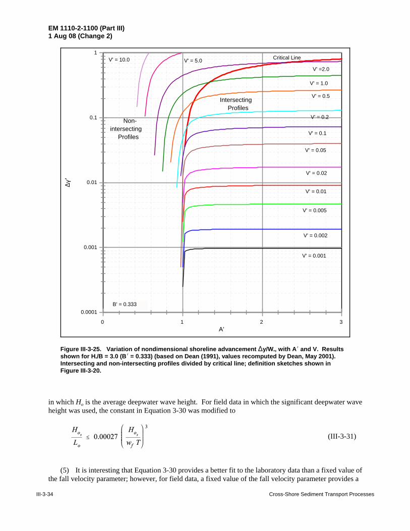
EM 1110-2-1100 (Part III)1 Aug 08 (Change 2)
III-3-34 Cross-Shore Sediment Transport Processes
0.0001
0.001
0.01
0.1
1
)(r
0 1 2 3 A'
V' = 0.001
V' = 0.002
V' = 0.005
V' = 0.01
V' = 0.02
V' = 0.05
V' = 0.1
V' = 0.2
V' = 0.5
V' = 1.0
V' =2.0V' = 5.0V' = 10.0
B' = 0.333
Non-intersecting
Profiles
IntersectingProfiles
Critical Line
Figure III-3-25. Variation of nondimensional shoreline advancement )y/W*, with AN and V. Resultsshown for H*/B = 3.0 (BN = 0.333) (based on Dean (1991), values recomputed by Dean, May 2001). Intersecting and non-intersecting profiles divided by critical line; definition sketches shown inFigure III-3-20.
(III-3-31)
in which Ho is the average deepwater wave height. For field data in which the significant deepwater waveheight was used, the constant in Equation 3-30 was modified to
(5) It is interesting that Equation 3-30 provides a better fit to the laboratory data than a fixed value ofthe fall velocity parameter; however, for field data, a fixed value of the fall velocity parameter provides a

EM 1110-2-1100 (Part III)1 Aug 08 (Change 2)
Cross-Shore Sediment Transport Processes III-3-35
0.0001
0.001
0.01
0.1
1
)(r
0 1 2 3 A'
V' = 0.001
V' = 0.002
V' = 0.005
V' = 0.01
V' = 0.02
V' = 0.05
V' = 0.1
V' = 0.2
V' = 0.5
V' = 1.0
V' =2.0V' = 5.0V' = 10.0
B' = 0.25
Non-intersecting
ProfilesIntersecting
Profiles
Critical Line
Figure III-3-26. Variation of nondimensional shoreline advancement )y/W*, with AN and V. Resultsshown for H*/B = 4.0 (BN = 0.25), based on Dean (1991), values recomputed by Dean, May 2001). Intersecting and non-intersecting profiles divided by critical line; definition sketches shown inFigure III-3-20.
(III-3-32)
better fit than Equation 3-30 (Kraus, Larson, and Kriebel 1991). Dalrymple (1992) has shown thatEquations 3-29 and 3-30 can be represented in terms of a single profile parameter P where
and that the criterion for bar formation is that P exceeds about 10,000.

EM 1110-2-1100 (Part III)1 Aug 08 (Change 2)
III-3-36 Cross-Shore Sediment Transport Processes
EXAMPLE PROBLEM III-3-2FIND:
The equilibrated additional dry beach width )y due to cross-shore transport.
GIVEN:DN = 0.2 mm, DF = 0.24 mm, B = 2 m, V = 400 m3/m.
H6 = 1.5 m, FH = 0.64 m as provided in WES and CEDRS databases discussed in Part II-8.
SOLUTION:Based on the above, the sediment scale parameters are determined from Figure III-3-18 and/or
Table III-3-3 to be: AN = 0.1 m1/3, AF = 0.11 m1/3. The effective wave height He is determined fromEquation 3-10 as:
He = H6 + 5.6 FH = 1.5 + (5.6)(0.64) – 5.1 m
The closure depth h* is determined from Equation 3-12 as:
h* = hC = 1.57 He = (1.57) (5.11) – 8 m
The reference width of effective motion W* is based on Equation 3-19
With this information, it is possible to determine the following nondimensional quantities:
BN = B/h* = 2/8 = 0.25, AN = AF/AN = 0.11/0.1 = 1.1
VN = V/(BW*) = 400/(2)(716) – 0.28
Since BN = 0.25, Figure III-3-26 is applicable and for AN = 1.1 and VN = 0.28, it is found that )yN = 0.092.Thus )y = (0.092)(716) – 65.9 m. Also, it is seen from Figure III-3-26 that this solution is near theboundary of the intersecting/nonintersecting profiles.The native and nourished profiles are shown inFigure III-3-27. The solution is next carried out with the appropriate equations for comparison with thegraphical procedure. Applying Equation 3-22 to determine whether the profiles will be intersecting ornonintersecting
compared with the applied VN of 0.28. Thus since VN<(VN)c1 the solution is an intersecting profile.Applying Equation 3-24 requires an iterative solution for )yN. This equation can be reduced to
0.28 = )yN + 9.20()yN)5/3
the solution to which yields )yN = 0.0955 or )y = 68.4 m(Continued)

EM 1110-2-1100 (Part III)1 Aug 08 (Change 2)
Cross-Shore Sediment Transport Processes III-3-37
Figure III-3-27. Nourishment with coarser sand than native (intersecting profiles)
Example Problem III-3-2 (Concluded)Thus, for this example, the graphical solution is reasonable. The calculated intersection distance forthe two profiles yI is determined from
or
and
By comparison, the corresponding values from the graphical solution are yI = 495 m and hI = 6.25 m.Figure III-3-27 presents the results of the graphical solution.

EM 1110-2-1100 (Part III)1 Aug 08 (Change 2)
III-3-38 Cross-Shore Sediment Transport Processes
EXAMPLE PROBLEM III-3-3FIND:
V, the volume of sand necessary to achieve the additional dry beach width )y of 50 m.
GIVEN:B=2 m, DN = DF = 0.25 mm, )y = 50 m, where H6=1.5 m, FH = 0.4 m.
SOLUTION:
The value of h* is computed as:
h* = 1.57 (H6 + 5.6 FH) = 1.57 [1.5 + (5.6)(0.4)] – 5.9 m
For these values, the associated A values are determined from Figure III-3-18 and/or Table III-3-3 to be:AN = AF = 0.115 m1/3. The reference width of active motion W* is
and the required nondimensional quantities are:
)y/W* – 50/367 – 0.136, BN = B/h* – 0.34, AN = AF/AN = 0.115/0.115 = 1.0
Since the value of BN lies between the two values represented in Figures III-3-24 and III-3-26, it isnecessary to interpolate. The values from these two figures are: VN(BN = 0.25) = 0.75, VN(BN = 0.5) =0.35. Interpolating linearly, VN is found to be 0.606 for the desired BN value of 0.34, from which thevolume V is determined as V = VN B W* = (0.606) (2) (367) – 445 m3/m. Since the fill and nativesediments are of the same size, it is clear that the two profiles will be nonintersecting and thatEquation 3-25 can be used to compute the nondimensional volume directly
(Continued)

EM 1110-2-1100 (Part III)1 Aug 08 (Change 2)
Cross-Shore Sediment Transport Processes III-3-39
Figure III-3-28. Example III-3-3. Nourishment with same-sized sand as native (nonintersectingprofiles)
Example Problem III-3-3 (Concluded)
which yields a volume of sand, V = VN B W* = (0.554)(2)(367) = 407 m3/m, which is about 9 percentless than the value determined by interpolating between the values from the two figures. Since inthis particular case, the two sand sizes are the same and thus every contour must be displaced by thesame amount, an approximate equation for the required volume density is the product of the contourdisplacement (50 m) and the full depth of active motion: V = ()y)(h* + B) = (50)(5.9 + 2) =395 m3/m. This result differs slightly from the values determined above because a small wedge-shaped sand volume has been neglected near the depth of closure. The native and nourished profilesare plotted in Figure III-3-28.

EM 1110-2-1100 (Part III)1 Aug 08 (Change 2)
III-3-40 Cross-Shore Sediment Transport Processes
Figure III-2-29. Illustration of effect of volume added V and fill sediment scaleparameter AF on additional dry beach width )y. Example conditions: B = 1.5 m,h* = 6 m, AN = 0.1 m1/3
EXAMPLE PROBLEM III-3-4FIND:
The variation in equilibrated dry beach width with volume added for three candidate fill sand sizes.
GIVEN:Three candidate borrow sites with representative sand sizes: = 0.15 mm, = 0.2 mm and
= 0.25 mm. The native sand size, DN = 0.2 mm. The berm height B = 1.5 m and h* = 6 m.
SOLUTION:The associated values of the sediment scale parameters are determined from Figure III-3-18 and/or
Table III-3-3: AN = 0.1 m1/3, = 0.084 m1/3, = 0.1 m1/3, and = 0.115 m1/3, respectively.
The procedures illustrated in Example Problems III-3-2 and III-3-3 produce the results shown inFigure III-3-29. It is seen that there is a nearly linear relationship for the sand that is of the same sizeas the native in accordance with: V =()y)(h* + B). For the fill sand, which is coarser than the native, forvolumes less than approximately 450 m3/m, the increase in dry beach width for each volume added isgreater than for the same-sized sand. For this region, the profiles are intersecting. For greater volumes,the profiles are nonintersecting and the slope of the relationship is nearly the same as for AF/AN = 1.0.For the sand smaller than the native, the profiles are submerged for the smaller volumes and later becomeemergent in accordance with Equation 3-23. For larger volumes, the relationship has approximately thesame slope as that for sand the same size as the native. The explanation for this is that once the profilesbecome emergent and nonintersecting, additional volumes of sand added simply displace the profile withall contours moving the same distance over the active depth. Thus the slope in Figure III-3-29 for thissituation is nearly independent of the grain size.

EM 1110-2-1100 (Part III)1 Aug 08 (Change 2)
Cross-Shore Sediment Transport Processes III-3-41
Figure III-3-30. Mean monthly shoreline position (A) and unit volume (B) at Jupiter Island, FL, referenced tofirst survey (Dewall and Richter 1977)

EM 1110-2-1100 (Part III)1 Aug 08 (Change 2)
III-3-42 Cross-Shore Sediment Transport Processes
Figure III-3-31. Changes in shoreline position and unit volume at Westhampton Beach,New York (Dewall 1979)
40t·~~ o~~
-40 40 o[ A..... .r
-40 [~\lv'\J~
4~[~j(Wf -40[
40 ~ E Ot··"'-.l '--" V'~Vf '{ c -40
.Q 40 +-' 'ii) 0 0 1----+---l--1---A~~-(L
<I)
c <I) L.
0 .c (/)
_j (/)
~
-40 40
0
-40 40
0
-40 40
o~~~~~~~~
-40 40
o~-----+~+---
-40 40
o~~------~~~
-40 40
O~+M----~--~~
-40~~~~~~~~
1962 1966 1968 1971 1974
Year
PROFILE LINE
2
3
4
150
otrvh~ -150 I
150
0 t F""'vot:Jf.----v..f -150
150
0 t .. -~ ,_rvv--150
Groin Construction
5
6
7
8
9
,-... E
"--.. -150 I")
E 150
m Or-~~-=~-----
~ -150 0 150 >
o~~~~~~~
-150 150
0~~~~~~--
-150 150
Ohd~~~~+----
Groins -150 and Fill--~15~0:::------------
10
11
ot, .... ~ tJb. ... \T~IJ\IV'
-150 150
-15~t I ~; I 1-t:'!::: 1962 1966 1968 1971 197
Year

EM 1110-2-1100 (Part III)1 Aug 08 (Change 2)
Cross-Shore Sediment Transport Processes III-3-43
(III-3-33)
h. Static models for shoreline response to sea level rise and/or storm effects.
(1) As water level and/or wave conditions change, the profile will respond toward a new equilibrium.If the conditions change very slowly, the profile changes will nearly maintain pace with the changedconditions and static models are applicable. However, rapidly changing conditions require dynamic modelsthat account for the time scales of response of the profile. This section presents several useful static modelsfor profile response.
(2) First, consider the long-term profile response to sea level rise. On a worldwide basis, the averagesea level has risen approximately 12 cm during the last century. However, the relative sea level changes(difference between absolute sea level rise and vertical land movements) at a particular location can differsubstantially from the average, ranging from locations at which the relative sea level (RSL) change is a riseof four times the average (Louisiana (Penland, Suter, and McBride 1987)) and locations where the RSLchange is decreasing at a rate of almost 1 m per century (Alaska (Hicks, Debaugh, and Hickman 1983)).Human-induced activities can cause considerable subsidence, primarily from extraction of ground fluidsand the consequent reduction of pore pressures (National Research Council 1984), and can be a reason forrelative sea level changes higher than average. Uplifting due to tectonic activity is the typical reason forrelative sea level changes lower than average. As noted previously, any rise in mean water level on a beachprofile that is otherwise in equilibrium must result in a redistribution of sand with erosion of the foreshoreand with deposition of sand offshore near the depth of closure to maintain the profile shape relative to therising water level. In the following discussion, equilibrium profile methods are applied to determineanalytical solutions for the shoreline recession, here denoted by the symbol R, which will be more convenientnotation than negative values of y.
(3) Bruun (1962) proposed the following relationship for equilibrium shoreline response R4 to sea levelrise S
in which L* and (h*+B) are the width and vertical extent of the active profile and the subscript “4” indicatesa static response. The basis for this equation is seen in Figure III-3-32 in which the two components of theresponse are: (1) a retreat of the shoreline R4, which produces a sediment “yield” R4(h* + B), and (2) anincrease in elevation of the equilibrium profile by an amount of the sea level rise S, which causes a sediment“demand” equal to SL*. Equating the demand and the yield results in Equation 3-33, which is known as the“Bruun Rule.” It is noted that the Bruun Rule does not depend on the particular profile shape.
(4) The Bruun Rule has been modified to account for several features of natural beaches that were notaccounted for in the original development. Bruun (1988), for example, shows that Equation 3-33 may bemodified to account for loss or “winnowing” of fine sediment out of the profile or for loss of sediment todeepwater canyons or other “sinks” in the offshore. Similar corrections may be made to account forunbalanced sediment flux into or out of the beach profile due to gradients in the net longshore sedimenttransport, as shown, for example, by Everts (1985).
(5) Despite these modifications, several aspects of the Bruun Rule have remained problematic. Forexample, the upper limit of the active profile is not clearly defined in Figure III-3-32 so that it is difficult toestablish a realistic profile width L* in Equation 3-33. Dean and Maurmeyer (1983) later extended Bruun'sresult to apply to the case of a barrier island in the form

EM 1110-2-1100 (Part III)1 Aug 08 (Change 2)
III-3-44 Cross-Shore Sediment Transport Processes
Figure III-3-32. Components of sand volume balance due to sea level rise and associated profileretreat according to the Bruun Rule
Ef fective Motion~
·--- ' ---
a) Volume of Sand "Generated" by Horizontal Retreat, Roo, of Equilibrium Profile Over Vertical Distance ( h * +8) r.- L.,.- --1-:
t ___ _ Depth of Effective Motion
b) Volume of Sand Required to Maintain an Equilibrium Profile of Active Width, L* , Due to a Rise, S, in Mean Water Level
Deposition
_j s_
Profile After Response to Sea Level Rise
. . -, ... ~.- . ' ...

EM 1110-2-1100 (Part III)1 Aug 08 (Change 2)
Cross-Shore Sediment Transport Processes III-3-45
(III-3-34)
Figure III-3-33. The Bruun Rule generalized for the case of a barrier island that maintains its form relative tothe adjacent ocean and lagoon (Dean and Maurmeyer 1983)
(III-3-35)
and the various terms are explained in Figure III-3-33. In general, the shoreline retreat is some 50 to200 times the sea level rise with the greater factors associated with the milder beach slopes and moreenergetic wave conditions (i.e., greater h*). These factors for the case of a barrier island would beconsiderably greater due to the difference term in the denominator (Equation 3-34). Situations where theregion behind the island is deep may explain the geological evidence for some barrier islands which arebelieved to have “drowned in place” rather than to have migrated landward.
(6) The Bruun Rule has been subjected to verifications both in the laboratory and in the field. Hands(1983), evaluated the Bruun Rule in Lake Michigan using 25 beach profiles over a 50-km length of shorelinesubjected to a 0.2-m water level rise over a 7-year period from 1969 to 1976. The on- and offshore limits ofprofile response were determined directly from measured beach profiles. Thus, the depth of closure wasidentified as the maximum depth of significant profile change observed from beach surveys. Likewise, theupper limit of profile change was selected as the natural vegetation line in the foredunes. With theseempirical input parameters, calculated profile retreat over the 7-year period then agreed to within 10 percentof measured values. Over shorter periods of time for example, over a 3-year period, Hands found that theBruun Rule initially over-estimated the profile response due to the time lag between elevated water levels andthe profile response. Storm processes were then identified as being responsible for causing rapid equilibrationof the profiles and for causing the profiles to “catch up” or equilibrate relative to the water level.
(7) Edelman (1972) modified the Bruun Rule to make it more appropriate for larger values of increasedwater levels and for time-varying storm surges. It was assumed that the profile maintained pace with therising sea level and thus, at each time, the following equation is valid

EM 1110-2-1100 (Part III)1 Aug 08 (Change 2)
III-3-46 Cross-Shore Sediment Transport Processes
(III-3-36)
Figure III-3-34. Elements of the Edelman model
(III-3-37)
where now B(t) represents the instantaneous total height of the active profile above the current water level.As shown in Figure III-3-34, B(t)=Bo-S(t) where Bo is the original berm height. For application to stormevents, Edelman also adopted the breaking depth hb (and surf zone width Wb) rather than the offshore depthof closure h* (and corresponding W*) as would be appropriate for long-term sea level rise. SubstitutingEquation 3-35 and integrating gives
(8) Using the small argument approximation for the natural logarithm, it is readily shown that to the firstapproximation, Edelman's equation is equivalent to the Bruun Rule.
(9) Dean (1991) derived similar solutions for storm-induced berm retreat based on theoretical pre- andpost-storm profile forms given by the equilibrium profile in Equation 3-14. Because pre- and post-stormprofiles were defined by an analytical form, the equilibrium beach response could be obtained by integratingthe areas (volume per unit length) between the initial and final equilibrium profiles and by equating theresulting eroded and deposited areas. Solutions were obtained for both the case of a uniform water level riseand for the case where breaking waves create a distribution of wave setup across the surf zone. Oneinteresting result is the case where water levels are elevated by both a storm surge and by breaking-inducedwave setup. For this case, an approximate solution for the steady-state erosion is given as
where Wb is the width of the surf zone, defined for the equilibrium profile as Wb = (hb/A)3/2. The solution forerosion due to combined storm surge and wave setup is similar in form to the Bruun Rule in Equation 3-33.In this case, wave setup causes a general rise in water level in the surf zone so that it functions much like

EM 1110-2-1100 (Part III)1 Aug 08 (Change 2)
Cross-Shore Sediment Transport Processes III-3-47
(III-3-38)
(III-3-39)
(III-3-40)
storm surge. It is noted, however, that storm surge has a much larger effect than wave setup. For this reason,the other analytical solutions that follow do not include wave setup effects and, instead, assume that beachresponse is driven primarily by storm surge.
(10) Kriebel and Dean (1993) considered both profiles with a vertical face at the water line as shown inFigure III-3-35a and profiles with a sloping beach face as shown in Figure III-3-35b. They showed that byaccounting for the small wedge-shaped sand volume offshore of the breaking depth, somewhat improvedexpressions could be developed for the potential beach recession due to elevated water levels. The beachprofile with a vertical face is a special limiting case of the profile with a sloping beach face, thus only theresults for the sloping beach face are given here. As shown by Kriebel and Dean (1993), the general resultfor equilibrium berm recession due to a storm surge level S is given as
where mo is the slope of the beach profile at the waterline. This slope is joined to the concave equilibriumprofile at a depth where the slope of the equilibrium profile is equal to mo. As a result, the surf zone widthcan be shown to be equal to
where yo is a small offset of the shoreline between the sloping beach face and the imaginary or virtual originof the equilibrium profile, given by yo = (4A3)/(27mo
3). For most conditions, this offset is negligible and canbe neglected when estimating the surf zone width, as will be illustrated in Example Problem III-3-6. Forengineering application, it is also of interest to compute the volume of sand eroded between the initial andfinal profiles per unit length of beach. For the case with a sloping beach face, the volume eroded from theberm above the initial still-water level due to a storm surge level S is given by
(11) When the beach face slope becomes infinite, the solutions from Equation 3-38 for the vertical beachface depicted in Figure III-3-35a are similar to those obtained by the Bruun Rule in Equation 3-33 or by Dean(1991) in Equation 3-37. The major difference is the term S/2 in the denominator of Equation 3-38, whichis the result of considering the small wedge-shaped volume of sand near the breakpoint. For more realisticbeach face slopes, the results in Equation 3-38 will yield smaller estimates of the potential berm recessionthan the Bruun or Dean solutions, since a portion of the rise in water level is accommodated by shifting theshoreline higher on the sloping beach face and less berm retreat is then required. Kriebel and Dean (1993)also provide analytical solutions for cases where the beach profile has a distinct dune on top of the berm.

EM 1110-2-1100 (Part III)1 Aug 08 (Change 2)
III-3-48 Cross-Shore Sediment Transport Processes
Figure III-3-35. Profile forms considered by Kriebel and Dean (1993)
Reo ~=(hb)3/2
A
VI 8 -
a) Profile with vertical beach face
B
b) Profile with sloping beach face

EM 1110-2-1100 (Part III)1 Aug 08 (Change 2)
Cross-Shore Sediment Transport Processes III-3-49
EXAMPLE PROBLEM III-3-5
FIND:The rate of shoreline retreat, according to the Bruun Rule, then find the rate at which beach
nourishment would be required to maintain the shoreline position.
GIVEN:
h* = 6 m, B = 2 m, D = 0.2 mm, and a rate of sea level rise of .
SOLUTION:
The sediment scale parameter is determined from Figure III-3-18 and/or Table III-3-3 as A =0.1 m1/3. The width W* of the active nearshore zone is determined from Equation 3-19 as
and from Equation 3-33, assuming the berm stays at a constant elevation, the rate of shoreline retreatis given by
so that the ratio of shoreline retreat to sea level rise is about 58.
When considering sea level rise and beach nourishment, from Equation 3-42, the rate at which sandmust be added to offset the erosion due to sea level rise is

EM 1110-2-1100 (Part III)1 Aug 08 (Change 2)
III-3-50 Cross-Shore Sediment Transport Processes
EXAMPLE PROBLEM III-3-6FIND:
The potential berm retreat, along with the volume of sand eroded from above the mean sea level,for the storm conditions given below.
GIVEN:Equilibrium beach profile with sand grain size D = 0.25 mm, beach face slope mo = 0.05, and
berm height B = 2 m. Storm conditions with a peak surge level S = 2 m and a breaking depth hb =3.0 m.
SOLUTION:The equilibrium berm retreat may be determined from Equation 3-38, which first requires
knowledge of the breaking depth hb and the surf zone width Wb, which, from Equation 3-39, are givenby Wb= yo+(hb/A)3/2. From Table III-3-3, the so-called A parameter for the equilibrium beach profileis found to be A = 0.115 m1/3 based on the grain size of 0.25 mm.
In calculating the surf zone width, the term (hb/A)3/2 is equal to (3.0m/0.115m1/3)3/2 = 133.2 m whilethe small shoreline offset is given by yo = (4A3)/(27mo
3) = 1.8 m. The total surf zone width is then Wb= 1.8 m + 133.2 m = 135.0 m. As noted, however, the offset is negligible and could be neglected forsimplicity.
From Equation 3-38, the potential berm retreat is now determined as
From Equation 3-40, the potential volume eroded from above the mean sea level datum is given by
These solutions are known to generally overestimate erosion associated with severe storms. Forexample, Chiu (1977) compared both the Edelman and Dean methods to erosion measured afterHurricane Eloise on the Florida coast and found that both methods gave erosion estimates that wereas much as a factor of 5 higher than observed. The reason for this overprediction is that thesemethods assume the profile responds instantly to changes in water level while they neglect thetransient or time-dependent approach to equilibrium. Such equilibrium solutions are still useful froman engineering perspective since they place a conservative upper bound on the actual beach response.
(12) While these idealized analytical solutions are useful, such computations of the maximum potentialresponse can also be performed numerically for a measured (surveyed) beach and dune profile. In this case,
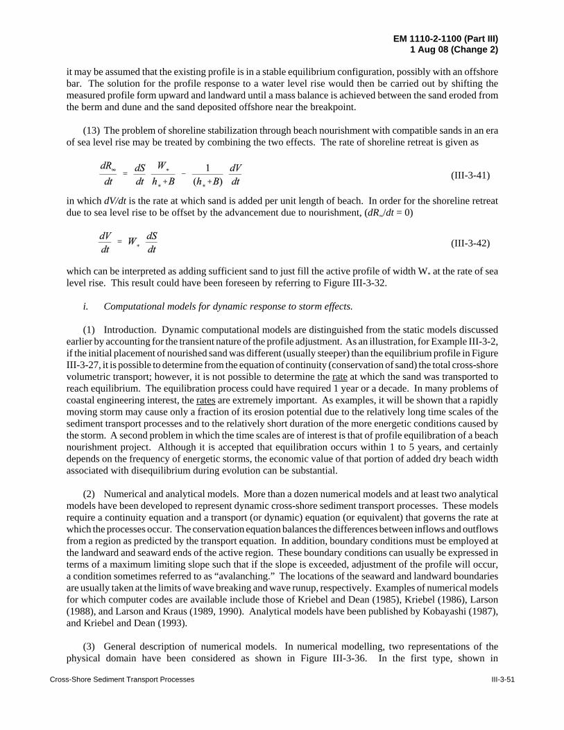
EM 1110-2-1100 (Part III)1 Aug 08 (Change 2)
Cross-Shore Sediment Transport Processes III-3-51
(III-3-41)
(III-3-42)
it may be assumed that the existing profile is in a stable equilibrium configuration, possibly with an offshorebar. The solution for the profile response to a water level rise would then be carried out by shifting themeasured profile form upward and landward until a mass balance is achieved between the sand eroded fromthe berm and dune and the sand deposited offshore near the breakpoint.
(13) The problem of shoreline stabilization through beach nourishment with compatible sands in an eraof sea level rise may be treated by combining the two effects. The rate of shoreline retreat is given as
in which dV/dt is the rate at which sand is added per unit length of beach. In order for the shoreline retreatdue to sea level rise to be offset by the advancement due to nourishment, (dR4/dt = 0)
which can be interpreted as adding sufficient sand to just fill the active profile of width W* at the rate of sealevel rise. This result could have been foreseen by referring to Figure III-3-32.
i. Computational models for dynamic response to storm effects.
(1) Introduction. Dynamic computational models are distinguished from the static models discussedearlier by accounting for the transient nature of the profile adjustment. As an illustration, for Example III-3-2,if the initial placement of nourished sand was different (usually steeper) than the equilibrium profile in FigureIII-3-27, it is possible to determine from the equation of continuity (conservation of sand) the total cross-shorevolumetric transport; however, it is not possible to determine the rate at which the sand was transported toreach equilibrium. The equilibration process could have required 1 year or a decade. In many problems ofcoastal engineering interest, the rates are extremely important. As examples, it will be shown that a rapidlymoving storm may cause only a fraction of its erosion potential due to the relatively long time scales of thesediment transport processes and to the relatively short duration of the more energetic conditions caused bythe storm. A second problem in which the time scales are of interest is that of profile equilibration of a beachnourishment project. Although it is accepted that equilibration occurs within 1 to 5 years, and certainlydepends on the frequency of energetic storms, the economic value of that portion of added dry beach widthassociated with disequilibrium during evolution can be substantial.
(2) Numerical and analytical models. More than a dozen numerical models and at least two analyticalmodels have been developed to represent dynamic cross-shore sediment transport processes. These modelsrequire a continuity equation and a transport (or dynamic) equation (or equivalent) that governs the rate atwhich the processes occur. The conservation equation balances the differences between inflows and outflowsfrom a region as predicted by the transport equation. In addition, boundary conditions must be employed atthe landward and seaward ends of the active region. These boundary conditions can usually be expressed interms of a maximum limiting slope such that if the slope is exceeded, adjustment of the profile will occur,a condition sometimes referred to as “avalanching.” The locations of the seaward and landward boundariesare usually taken at the limits of wave breaking and wave runup, respectively. Examples of numerical modelsfor which computer codes are available include those of Kriebel and Dean (1985), Kriebel (1986), Larson(1988), and Larson and Kraus (1989, 1990). Analytical models have been published by Kobayashi (1987),and Kriebel and Dean (1993).
(3) General description of numerical models. In numerical modelling, two representations of thephysical domain have been considered as shown in Figure III-3-36. In the first type, shown in

EM 1110-2-1100 (Part III)1 Aug 08 (Change 2)
III-3-52 Cross-Shore Sediment Transport Processes
(III-3-43)
(III-3-44)
(III-3-45)
(III-3-46)
Figure III-3-36a, the cells are finite increments of the distance variable y. Thus the distance is theindependent variable and the dependent variable is depth, which varies with time. In the second type shownin Figure III-3-36b, the computational cells are formed by finite increments of the depth h. In this case, theindependent variable is h and y varies with time for each h value. There is an inherent advantage of the firsttype since the presence of bars can be represented with no difficulties. All dynamic models require acontinuity equation and a transport (dynamic) equation.
(a) Conservation equation. The conservation equation is very straightforward and for the computationalcell type in Figure III-3-36a is given by
in which y and t are the independent variables. If h and t are regarded as the independent variables as inFigure III-3-36b, the conservation equation is
in which it is noted that for each depth value (h), there is an associated distance value (y).
(b) Transport relationships. Sediment transport relationships fall within the categories of “closed loop,”which converge to a target profile and “open loop,” which are not a priori constrained to the final(equilibrium) profile. Transport relationships of the “closed loop” type will be reviewed first.
(c) Closed loop transport relationships. One of the first closed loop transport relationships was thatproposed by Kriebel and Dean (1985). Recalling that the equilibrium beach profile (EBP) represented byEquation 3-14 is consistent with uniform wave energy dissipation per unit water volume D*, Kriebel and Deanadopted a simple transport relationship in the form
such that at equilibrium D=D*, and an equilibrium profile results. The parameter KN is then used to calibratethe model by correlating the sediment transport rate to the excess energy dissipation. The transportrelationship above may be modified to be consistent with a profile with beach face slope mo
where , is an additional model parameter as suggested by Larson and Kraus (1989). In this expression, thecalibration parameter KNN differs from that used in Equation 3-45, since the additional gravitational effects,represented by the slope term, assist in moving sediment offshore.
(d) Open loop transport relationships. These transport relationships depend on the detailedhydrodynamics and attempt to incorporate the actual processes more faithfully than the closed loop variety.Usually both bed load and suspended load transport components are represented based on the hydrodynamicproperties averaged over a wave period. Open loop models will not be considered further in this chapter;however, an excellent review of open loop models is given by Roelvink and Broker (1993). In general, thesemodels can be grouped according to the physical processes that are assumed to be dominant for cross-shore
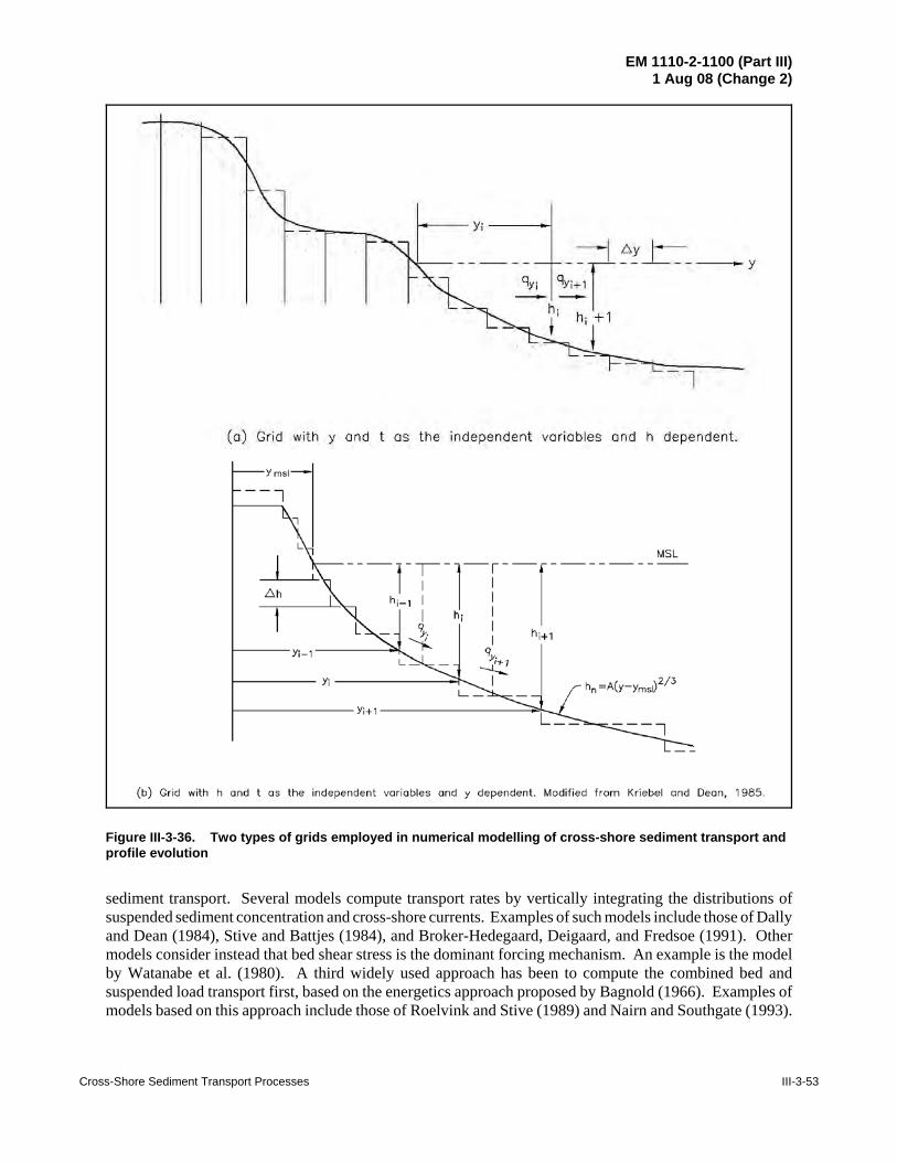
EM 1110-2-1100 (Part III)1 Aug 08 (Change 2)
Cross-Shore Sediment Transport Processes III-3-53
Figure III-3-36. Two types of grids employed in numerical modelling of cross-shore sediment transport andprofile evolution
sediment transport. Several models compute transport rates by vertically integrating the distributions ofsuspended sediment concentration and cross-shore currents. Examples of such models include those of Dallyand Dean (1984), Stive and Battjes (1984), and Broker-Hedegaard, Deigaard, and Fredsoe (1991). Othermodels consider instead that bed shear stress is the dominant forcing mechanism. An example is the modelby Watanabe et al. (1980). A third widely used approach has been to compute the combined bed andsuspended load transport first, based on the energetics approach proposed by Bagnold (1966). Examples ofmodels based on this approach include those of Roelvink and Stive (1989) and Nairn and Southgate (1993).

EM 1110-2-1100 (Part III)1 Aug 08 (Change 2)
III-3-54 Cross-Shore Sediment Transport Processes
(III-3-47)
(III-3-48)
(III-3-49)
(4) General description of analytical models.
(a) The analytical model of profile evolution by Kobayashi (1987) incorporates the conservation andtransport relationships (Equations 3-41 and 3-43). The transport equation is linearized such that a diffusionequation results. The landward and seaward receding and advancing limits of the evolving profile are treatedas moving boundary conditions. Kobayashi (1987) presents an analytical solution for the case of a constantelevated water level in the form of fairly complex error functions. For more complete water level scenarios,a numerical scheme must be used. As presented, the model does not lend itself readily to engineeringapplications.
(b) A simpler analytical model for predicting dynamic profile response during storms is the so-calledConvolution Method of Kriebel and Dean (1993). This method is based on the observation that beaches tendto respond toward a new equilibrium exponentially over time. For laboratory conditions, where a beach issuddenly subjected to steady wave action, the time-dependent shoreline response R(t) may be approximatedby the form
where R4 is the equilibrium beach response and TS is the characteristic time-scale of the system. Anexponential response of this kind has been observed in wave tank experiments by Swart (1974), Dette andUliczka (1987), and Larson and Kraus (1989).
(c) A more general result for the dynamic erosion response may be obtained by noting thatEquation 3-47 suggests that the rate of profile response is proportional to the difference between theinstantaneous profile form and the ultimate equilibrium form. An approximate differential equationgoverning the profile response to time-dependent variations in water level may be assumed in the form
where f(t) represents a unit-amplitude function of time that describes the storm surge hydrograph, while R4represents the equilibrium beach response for the peak water level. The general solution to this system maybe expressed as a convolution integral as
(d) As a result, several important characteristics of dynamic beach profile response are evident. First,a beach has a certain “memory,” so that the beach response at any one time is dependent on the forcingconditions applied over some preceding time period. As a result, the beach response will lag behind theerosion forcing. In addition, because of the exponential response characteristics of the beach system, thebeach response will be damped so that the actual maximum response will be less than the erosion potentialof the system.

EM 1110-2-1100 (Part III)1 Aug 08 (Change 2)
Cross-Shore Sediment Transport Processes III-3-55
(III-3-50)
(III-3-52)
j. Example application of an analytical model.
(1) Of the two analytical models, the Kriebel and Dean (1993) analytical model is simpler to apply andthus will be discussed and illustrated by several examples herein.
(2) A useful application of the convolution method is to analyze the erosion associated with an idealizedstorm surge hydrograph. Consider the case where the storm surge is approximated by the function
with F= B/TD and where TD is the total storm surge duration. The maximum storm surge level S would beused to determine the maximum potential erosion R4 according to Equation 3-38 or one of the otherexpressions for static profile response developed in the preceding section. As shown by Kriebel and Dean(1993), solution of the convolution integral in Equation 3-49, with the unit-amplitude forcing term f(t) equalto the sine-squared function, gives the following time-dependent erosion response
(III-3-51)
where $ is the ratio of the erosion time scale to the storm duration, which is given as $=2BTS/TD. Thepredicted beach response is shown in Figure III-3-37 for two different values of $, correspondingapproximately to a short-duration hurricane ($ = 10.6) and to a long-duration northeaster ($ = 0.76). Theexamples illustrate the role of storm duration in determining the maximum erosion response such that short-duration storms may only achieve a small percentage of their potential equilibrium response.
(3) The magnitude of the beach response from the sine-squared storm surge can be summarized in termsof the expected maximum dynamic erosion relative to the potential static or equilibrium response. This maybe shown to be a function of $, as illustrated in Figure III-3-38. In general, short-duration storms fall to theright of this curve such that the predicted maximum erosion may be only 20 to 40 percent of the maximumerosion potential. For long-duration storms, the maximum erosion may be from 40 to 90 percent of themaximum erosion potential. When the storm duration is equal to the erosion time scale, ($ = 2B), thedynamic erosion response is only 36 percent of the static response.
(4) The time scale of dynamic profile response TS has not been as widely considered in coastalengineering as the equilibrium erosion R4 and, thus far, the time scale has not been derived analytically. Asa result, empirical descriptions of the time scale are required. These have been developed from results of thenumerical erosion model of Kriebel (1986, 1990) for various combinations of profile geometry and breakingwave conditions. From these numerical tests, it was found that the time scale was approximately independentof the storm surge level, but varied strongly with sediment size (through the A parameter) and breaking waveheight, and varied less significantly as a function of beach profile geometry. Numerical results were analyzedby dimensional analysis to arrive at the following empirical relationship
(5) In Figure III-3-39, the numerically generated values of the erosion time scale are plotted as afunction of the expression on the right-hand side of the equation (above). In general, beaches composed of

EM 1110-2-1100 (Part III)1 Aug 08 (Change 2)
III-3-56 Cross-Shore Sediment Transport Processes
Figure III-3-37. Examples of profile response to idealized sine-squared stormsurge: (a) Short-duration hurricane, and (b) Long-duration northeaster (Kriebel andDean 1993)
EQUILIBRIUM RESPONSE
0.8 BETA=O
0.6
0.4
0.2
0
0.8
0.6
0.4
0 .2
0
.,.,...
0.785
EQUILIBRIUM RESPONSE BETA=O
0.785
BETA=1 0.6 ~--.,.,...
.,.,... .,.,... .,.,...
1.57
1r (radians) (a)
.........
" BETA=0.76
1.57
1r (radians) (b)
2.355
\ \ \
2.355
\ \
\
3.14
\ '\
3.14

EM 1110-2-1100 (Part III)1 Aug 08 (Change 2)
Cross-Shore Sediment Transport Processes III-3-57
Figure III-3-38. Maximum relative erosion versus ratio of storm duration toprofile time scale, TD/TS
Figure III-3-39. Empirical relationship for determination of erosion time scale,Ts

EM 1110-2-1100 (Part III)1 Aug 08 (Change 2)
III-3-58 Cross-Shore Sediment Transport Processes
EXAMPLE PROBLEM III-3-7FIND:
The shoreline recession, R(t), as a function of time and quantify the maximum erosion, Rmax.
GIVEN:Hb = 3 m, hb = 3.85m, D = 0.2 mm, B = 2 m, mo = 1:10, TD = 10 hr, and Smax = 1.5 m.
SOLUTION:
As in previous examples, the value of the profile scale parameter is determined from Figure III-3-18and/or Table III-3-3 as 0.1 m1/3. The active width of the surf zone Wb is calculated from Equation 3-19as
The equilibrium value of the shoreline response based on the maximum water level Smax is determinedfrom Equation 3-38 as
The morphological time scale Ts is determined from Figure III-3-39 by calculating the value of theabscissa in Figure III-3-39 as
(Continued)

EM 1110-2-1100 (Part III)1 Aug 08 (Change 2)
Cross-Shore Sediment Transport Processes III-3-59
Figure III-3-40. Potential and actual shoreline response based on Kriebel and Dean (1993) model
Example Problem III-3-7 (Concluded)
The morphological time scale is determined from Figure III-3-39 to be approximately 17.0 hr. The time-varying shoreline recession is determined from Equation 3-49 and is presented in Figure III-3-40. Themaximum erosion can be determined from Equation 3-49 or directly from Figure III-3-40 as Rmax/R4 =0.236 or Rmax = 13.9 m.
very fine sand, subjected to very large breaking wave heights, have extremely long time scales such that theywill experience only a small percentage of their equilibrium erosion potential during a typical storm.
k. Examples of numerical models.
(1) The numerical model described by Kriebel and Dean (1985) and later Kriebel (1986, 1990), was thefirst widely used numerical model developed to simulate storm-induced erosion based on equilibrium beachprofile concepts. This model assumes that a beach profile will evolve toward an equilibrium form in response

EM 1110-2-1100 (Part III)1 Aug 08 (Change 2)
III-3-60 Cross-Shore Sediment Transport Processes
(III-3-53)
(III-3-54)
to changing water levels and wave conditions and that the sediment transport rate is proportional to the“disequilibrium” existing between the profile at any instant in time and the equilibrium profile form.
This is quantified in terms of the “excess” energy dissipation per unit volume in the surf zone, as given byEquation 3-45. The energy dissipation per unit volume at any location in the surf zone is given by
where the last form is based on the assumption of shallow-water breaking waves. Based on the equilibriumbeach profile given by Equation 3-14, the equilibrium energy dissipation per unit volume is given by
where the equilibrium profile parameter A is determined either from the sediment grain size, as suggested inTable III-3-3 or from a best-fit of the equilibrium profile equation h = Ay2/3 to the measured beach profile.
(2) The numerical solution for profile response is based on a finite difference solution to the sedimentconservation equation given in Equation 3-44. In this case, the profile is gridded in a “stair-step” form asshown in Figure III-3-36(b) so that erosion or accretion (retreat or advance) of each elevation contour isdetermined by vertical gradients in the sediment transport rate. At each time-step, the local depth h inEquation 3-53 is the depth to the sand bed below the time-varying storm surge. As a result, beach profilechange is driven primarily by changes in water level associated with storm surge. Breaking waves are treatedvery simply by shallow-water, spilling-breaker assumptions and, as a result, have a secondary effect onprofile response. In effect, the breakpoint serves to separate the two main computational domains in themodel: the offshore region, where the sediment transport rate is assumed to equal zero, and the surf zone,where the transport rate is given by Equation III-3-45.
(3) In this model, an increase in water level due to storm surge allows waves to break closer to shore,thus temporarily decreasing the width of the surf zone and increasing the energy dissipation per unit volumeabove the equilibrium level. According to Equation III-3-45, this leads to offshore directed sediment trans-port, the gradients of which cause erosion of the foreshore, deposition near the breakpoint, and an overallwidening of the profile toward a new equilibrium form. At each time-step in the finite-difference solution,the profile responds toward equilibrium, but this is rarely, if ever, achieved due to the limited storm durations.
(4) The transport relationship used in the Kriebel and Dean model, given by Equation 3-45, requirescalibration of a single empirical parameter KN. Kriebel (1986) first determined this parameter from numericalsimulations of both large wave tank tests and hurricane-induced beach profile change as observed inHurricane Eloise on the Gulf Coast of Florida. Figure III-3-41 shows numerical profile development alongwith results of large wave tank tests of Saville (1957). This illustrates the time-dependent profiledevelopment. It is noted that in the offshore region near the breakpoint, numerical results appear reasonable;however, the model does not simulate bar and trough features. For the Hurricane Eloise data, one profile wascalibrated and the calibrated model was then applied to 20 additional profiles. Overall results showed thatthe model was capable of predicting the volume eroded from the dune to within about 25 to 40 percent, withlittle bias toward either under- or overestimating the volume eroded. Figure III-3-42 shows numerical modelsimulation of a long-duration extra-tropical storm from Point Pleasant, New Jersey. In these cases, measured

EM 1110-2-1100 (Part III)1 Aug 08 (Change 2)
Cross-Shore Sediment Transport Processes III-3-61
Figure III-3-41. Example of Kriebel and Dean erosion model calibration using large-wave tank dataof Saville (1957) (from Kriebel 1990)
Figure III-3-42. Comparison of Kriebel and Dean erosion model to measured profiles from northeast stormat Point Pleasant, NJ (from Kriebel 1990)

EM 1110-2-1100 (Part III)1 Aug 08 (Change 2)
III-3-62 Cross-Shore Sediment Transport Processes
(III-3-55)
post-storm profiles show evidence of post-storm beach recovery, which is not predicted in the numericalmodel.
An earlier version of the Kriebel and Dean model is provided in the ACES software package (Leenknecht,Szuwalski, and Sherlock 1992).
(5) The numerical model by Larson (1988) and Larson and Kraus (1989, 1990), SBEACH, isconceptually similar to the model of Kriebel and Dean (1985) but contains a more detailed description ofbreaking wave transformation and sediment transport across the beach profile, especially near the breakpoint.This model approximates the equation for conservation of sand in Equation 3-43 in finite difference formbased on the profile gridding depicted in Figure III-3-36(a). Thus, vertical changes in water depth aredetermined by horizontal gradients in sediment transport rate. In contrast to the Kriebel and Dean model, thisallows simulation of breakpoint bar formation and evolution.
(6) In the Larson and Kraus model, sediment transport rates in the surf zone are generally determinedby Equation 3-46 in terms of excess energy dissipation, but with an additional effect of the local bottomslope. Because of this additional term, Equation 3-46 requires calibration through adjustment of twoparameters, KNN and ,. The breaking wave model employed in the Larson and Kraus model is moresophisticated than that used by Kriebel and Dean, and is based on the breaking wave model of Dally, Dean,and Dalrymple (1985). This breaking wave model introduces gradients in the breaking wave height andenergy dissipation that, in turn, lead naturally to gradients in sediment transport that produce bar/troughformations. Because of this improved breaking wave model, beach profile changes can be driven by changesin wave conditions, in addition to changes in water level.
(7) The computational domain used in the Larson and Kraus model is divided into four regions acrossthe beach profile and the exact sediment transport relationship is adjusted somewhat for each of the fourregions. In the surf zone, which is the major region for cross-shore sediment transport in the model, transportdirections are first determined from the following critical value of wave steepness
which is recognized as Equation 3-30 presented earlier. At each time-step in the solution, if the actual valueof wave steepness exceeds the critical value given above, then transport is directed offshore over the entireactive profile. Transport is then onshore if wave steepness is smaller than this critical value. Transportmagnitudes in the surf zone are then determined by Equation 3-44, although the transport is “turned off” ifthe wave energy dissipation is below a critical value since this might cause a reversal in transport directionin conflict with the transport direction determined from wave steepness. It is noted, however, that therelationship determining transport direction (Equation 3-53) does not include any of the profilecharacteristics. In some cases where the profile is very steep, as may occur after beach nourishment, forexample, the transport direction utilized in the model may be onshore based on wave and sedimentcharacteristics whereas the actual transport would likely be offshore, even under mild wave conditions, dueto the artificially high profile slope.
(8) The Larson and Kraus model has been compared with laboratory and field data as shown inFigures III-3-43 and III-3-44. Figure III-3-43 presents results for the two sets of available large-scale wavetank data. The upper panel shows a comparison from the Saville (1957) data and the comparisons includecalculations at various times and the measured profile at 40 hr. The lower panel is for data from the Japanlarge tank and presents calculations at various times and the measured profile at 30-1/2 hr. The calculations

EM 1110-2-1100 (Part III)1 Aug 08 (Change 2)
Cross-Shore Sediment Transport Processes III-3-63
Figure III-3-43. SBEACH compared to two tests from large-scale wave tanks (Larson and Kraus1989)
3 ,--,
E '-/
I
-1
r--...
E '-/
I I-
-3 D.... w 0
-5
3
I
-1
I -3 I-D.... w 0
-5
CE Case 400 H
Distance Offshore (m)
60 80 100 calculated (hr)
(a) Test from large Beach Erosion Board tank.
CRIEPI Case 6-2
H
Dista nee Offshore (m)
60 80 100 calculated (hr)
(b) Test from large Japanese tank.

EM 1110-2-1100 (Part III)1 Aug 08 (Change 2)
III-3-64 Cross-Shore Sediment Transport Processes
Figure III-3-44. SBEACH tested against profile evolution data from Duck, NC (Larson and Kraus1989)
4
3 ;--....
E '-"'
2
-1
8
4
Duck, NC Calibration Interval No. 4
Wave
Wave Height
.....--. (.J (1.) QJ
'--"
10:55 840406
o) Input measured wove height, wove period end water level
Duck, NC Calibration Interval No. 4
LEGEND ---measured initial (840403)
-- calculated (840406)
-measured (840406)
Distance Offshore (m)
~ 0~------~.---------~------~--------~--------~------~ a.. (1.)
0
-4
100 150
b) Result of simulation
200 250 300
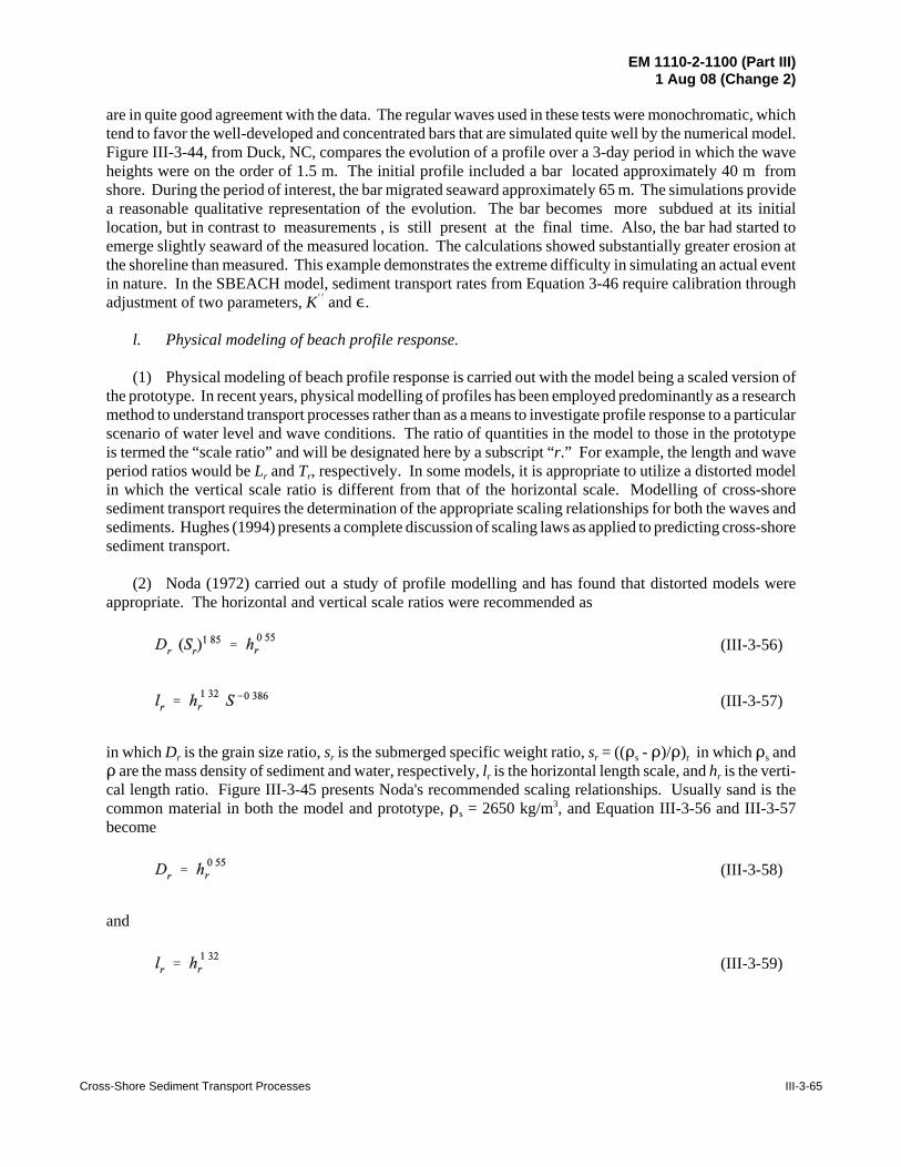
EM 1110-2-1100 (Part III)1 Aug 08 (Change 2)
Cross-Shore Sediment Transport Processes III-3-65
(III-3-56)
(III-3-57)
(III-3-58)
(III-3-59)
are in quite good agreement with the data. The regular waves used in these tests were monochromatic, whichtend to favor the well-developed and concentrated bars that are simulated quite well by the numerical model.Figure III-3-44, from Duck, NC, compares the evolution of a profile over a 3-day period in which the waveheights were on the order of 1.5 m. The initial profile included a bar located approximately 40 m fromshore. During the period of interest, the bar migrated seaward approximately 65 m. The simulations providea reasonable qualitative representation of the evolution. The bar becomes more subdued at its initiallocation, but in contrast to measurements , is still present at the final time. Also, the bar had started toemerge slightly seaward of the measured location. The calculations showed substantially greater erosion atthe shoreline than measured. This example demonstrates the extreme difficulty in simulating an actual eventin nature. In the SBEACH model, sediment transport rates from Equation 3-46 require calibration throughadjustment of two parameters, KNN and ,.
l. Physical modeling of beach profile response.
(1) Physical modeling of beach profile response is carried out with the model being a scaled version ofthe prototype. In recent years, physical modelling of profiles has been employed predominantly as a researchmethod to understand transport processes rather than as a means to investigate profile response to a particularscenario of water level and wave conditions. The ratio of quantities in the model to those in the prototypeis termed the “scale ratio” and will be designated here by a subscript “r.” For example, the length and waveperiod ratios would be Lr and Tr, respectively. In some models, it is appropriate to utilize a distorted modelin which the vertical scale ratio is different from that of the horizontal scale. Modelling of cross-shoresediment transport requires the determination of the appropriate scaling relationships for both the waves andsediments. Hughes (1994) presents a complete discussion of scaling laws as applied to predicting cross-shoresediment transport.
(2) Noda (1972) carried out a study of profile modelling and has found that distorted models wereappropriate. The horizontal and vertical scale ratios were recommended as
in which Dr is the grain size ratio, sr is the submerged specific weight ratio, sr = ((Ds - D)/D)r in which Ds andD are the mass density of sediment and water, respectively, lr is the horizontal length scale, and hr is the verti-cal length ratio. Figure III-3-45 presents Noda's recommended scaling relationships. Usually sand is thecommon material in both the model and prototype, Ds = 2650 kg/m3, and Equation III-3-56 and III-3-57become
and
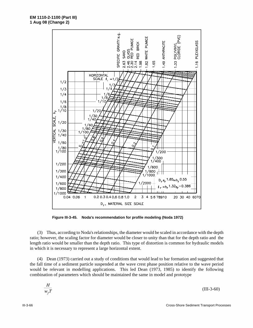
EM 1110-2-1100 (Part III)1 Aug 08 (Change 2)
III-3-66 Cross-Shore Sediment Transport Processes
Figure III-3-45. Noda's recommendation for profile modeling (Noda 1972)
(III-3-60)
(3) Thus, according to Noda's relationships, the diameter would be scaled in accordance with the depthratio; however, the scaling factor for diameter would be closer to unity than that for the depth ratio and thelength ratio would be smaller than the depth ratio. This type of distortion is common for hydraulic modelsin which it is necessary to represent a large horizontal extent.
(4) Dean (1973) carried out a study of conditions that would lead to bar formation and suggested thatthe fall time of a sediment particle suspended at the wave crest phase position relative to the wave periodwould be relevant in modelling applications. This led Dean (1973, 1985) to identify the followingcombination of parameters which should be maintained the same in model and prototype

EM 1110-2-1100 (Part III)1 Aug 08 (Change 2)
Cross-Shore Sediment Transport Processes III-3-67
(III-3-61)
(III-3-62)
(5) This combination of terms will be termed herein as the “Fall Velocity Parameter” (FVP). It wasfurther suggested that an appropriate model for cross-shore sediment transport is one based on undistortedFroude modelling for the wave characteristics and one that maintains the FVP the same in the model andprototype. This simple approach leads to the following requirement for scaling the sediment fall velocity wf
which is the standard relationship for velocity scaling for a Froude model.
(6) Evaluation of cross-shore modelling according to the FVP has been carried out by Vellinga (1983),Kriebel, Dally, and Dean (1986) and Hughes and Fowler (1990). Each of these studies concluded that theFVP was effective in scaling the erosion process. Figures III-3-46 and III-3-47, from Kriebel, Dally, andDean (1986) and Hughes and Fowler (1990), compare different scales while maintaining the same FVP inmodel and prototype. Considering the FVP as valid leads to the following valuable transport relationship fornumerical models
(7) One limitation for scaling by the FVP is that the length ratio Lr and the prototype diameter can resultin designated model sediments so small that cohesive forces would be significant. Although there are no strictguidelines for a minimum sediment size, values smaller than approximately 0.08 to 0.09 mm should beavoided.

EM 1110-2-1100 (Part III)1 Aug 08 (Change 2)
III-3-68 Cross-Shore Sediment Transport Processes
Figure III-3-46. Profile evolution by small- and large-scale wave tank tests. Basedon maintaining the same fall velocity parameter. Length ratio = 1:9.6 (Kriebel, Dally,and Dean 1986)
cm~:L' 0 100 200
em
Model H= 16.7 em, T= 1.8 s
--- Prototy pe H= 1.6 m, T=5.6 s
Prototype Elapsed Time=1.0 hr
3.0 hrs
5.0 hrs
10.0 hrs
20.0 hrs
30.0 hrs

EM 1110-2-1100 (Part III)1 Aug 08 (Change 2)
Cross-Shore Sediment Transport Processes III-3-69
Figure III-3-47. Profile evolution by small- and large-scale wave tank tests. Case of sloping seawall. Basedon maintaining the same fall velocity parameter. Length ratio = 1:7.5 (Hughes and Fowler 1990)
III-3-4. References
Bagnold 1940Bagnold, R. A. 1940. “Beach Formation by Waves: Some Model Experiments in a Wave Tank,” Journalof the Institution of Civil Engineers, Vol 15, pp 27-52.
Bagnold 1966Bagnold, R. A. 1966. “An Approach to the Sediment Transport Problem from General Physics,”U.S. Geological Survey Professional Paper 422-I, U. S. Dept of Interior.
Bailard 1981Bailard, J. A. 1981. “An Energetics Total Load Sediment Transport Model for a Plane Sloping Beach,”Journal of Geophysical Research, Vol 86, No. C11, pp 10938-10954.
Barnett and Wang 1988Barnett, M., and Wang, H. 1988. “Effects of a Vertical Seawall on Profile Response,” American Society ofCivil Engineers, Proceedings of the Twenty-first International Conference on Coastal Engineering,Chapter 111, pp 1493-1507.

EM 1110-2-1100 (Part III)1 Aug 08 (Change 2)
III-3-70 Cross-Shore Sediment Transport Processes
Birkemeier 1984Birkemeier, W. A. 1984. “Time Scales of Nearshore Profile Change,” Proceedings, 19th InternationalConference on Coastal Engineering, Chapter 102, pp 1501-1521.
Birkemeier 1985Birkemeier, W. A. 1985. “Field Data on Seaward Limit of Profile Change,” Journal of the Waterways, PortCoastal and Ocean Engineering, American Society of Civil Engineers, Vol 111, No. 3, pp 598-602.
Bodge 1992Bodge, K. R. 1992. “Representing Equilibrium Beach Profiles with an Exponential Expression,” Journal ofCoastal Research, Vol 8, No. 1, pp 47-55.
Broker-Hedegaard, Deigaard, and Fredsoe 1991Broker-Hedegaard, I., Deigaard, R., and Fredsoe, J. 1991. “Onshore/Offshore Sediment Transport andMorphological Modelling of Coastal Profiles,”Proceedings Coastal Sediments '91 Conference, pp 643-657.
Bruun 1954Bruun, P. 1954. “Coast Erosion and the Development of Beach Profiles,” Beach Erosion Board TechnicalMemorandum No. 44, U.S. Army Engineer Waterways Experiment Station, Vicksburg, MS.
Bruun 1962Brunn, P. 1962. “Sea-Level Rise as a Cause of Shore Erosion,” Journal of Waterways and Harbor Division,American Society of Civil Engineers, Vol 88, pp 117-130.
Bruun 1988Bruun, P. 1988. “The Bruun Rule of Erosion by Sea Level Rise: A Discussion on Large-Scale Two- andThree-Dimensional Usages,” Journal of Coastal Research, Vol 4, No. 4, pp 627-648.
Chiu 1977Chiu, T. Y. 1977. “Beach and Dune Response to Hurricane Eloise of September 1975. Proceedings ofCoastal Sediments '77, pp 116-134.
Clausner, Birkemeier, and Clark 1986Clausner, J. E., Birkemeier, W. A., and Clark, G. R. 1986. “Field Comparison of Four Nearshore SurveySystems,” Miscellaneous Paper CERC-86-6, U.S. Army Engineer Waterways Experiment Station, Vicksburg,MS.
Dally and Dean 1984Dally, W. R., and Dean, R. G. 1984. “Suspended Sediment Transport and Beach Profile Evolution,” Journalof Waterway, Port, Coastal, and Ocean Engineering, Vol 110, No. 1, pp 15-33.
Dally, Dean, and Dalrymple 1985Dally, W. R., Dean, R. G., and Dalrymple, R. G. 1985. “Wave Height Variation Across Beaches of ArbitraryProfile,” Journal of Geophysical Research, Vol 90, No. C6, pp 11917-11927.
Dalrymple 1992Dalrymple, R. A. 1992. “Prediction of Storm/Normal Beach Profiles,” Journal of Waterways, Port, Coastaland Ocean Engineering, American Society of Civil Engineers, Vol 118, No. 2, pp 193-200.

EM 1110-2-1100 (Part III)1 Aug 08 (Change 2)
Cross-Shore Sediment Transport Processes III-3-71
Dean 1973Dean, R. G. 1973. “Heuristic Models of Sand Transport in the Surf Zone,” Proceedings, Conference onEngineering Dynamics in the Surf Zone, Sydney, Australia.
Dean 1977Dean, R. G. 1977. “Equilibrium Beach Profiles: U.S. Atlantic and Gulf Coasts,” Department of CivilEngineering, Ocean Engineering Report No. 12, University of Delaware, Newark, DE.
Dean 1985Dean, R. G. 1985. “Physical Modelling of Littoral Processes,” Physical Modelling in Coastal Engineering,R. A. Dalrymple, ed., A. A. Balkema, pp 119-139.
Dean 1987aDean, R. G. 1987a. “Additional Sediment Input into the Nearshore Region,” Shore and Beach, Vol 55,Nos. 3-4, pp 76-81.
Dean 1987bDean, R. G. 1987b. “Coastal Sediment Processes: Toward Engineering Solutions,” Coastal Sediments '87,American Society of Civil Engineers, New Orleans, LA, Vol 1, pp 1-24.
Dean 1991Dean, R. G. 1991. “Equilibrium Beach Profiles: Characteristics and Applications,” Journal of CoastalResearch, Vol 7, No. 1, pp 53-84.
Dean and Dalrymple 1991Dean, R. G., and Dalrymple, R. A. 1991. Water Wave Mechanics for Engineers and Scientists, WorldScientific Pub. Co., Teaneck, NJ.
Dean and Dalrymple 2001Dean, R. G., and Dalrymple, R. A. 2001. Coastal Processes with Engineering Applications, CambridgeUniversity Press, New York.
Dean and Maurmeyer 1983Dean, R. G., and Maurmeyer, E. M. 1983. “Models for Beach Profile Response,” CRC Handbook on BeachErosion and Coastal Processes, P. D. Komar, ed., Chapter 7, pp 151-166.
Dette and Uliczka 1987Dette, H., and Uliczka, K. 1987. “Prototype Investigation on Time-Dependent Dune Recession and BeachErosion,” Proceedings Coastal Sediments '87, New Orleans, pp 1430-1444.
Dewall 1979Dewall, A. E. 1979. “Beach Changes at Westhampton Beach, New York,” MR 79-5, Coastal EngineeringResearch Center, U.S. Army Engineer Waterways Experiment Station, Vicksburg, MS.
Dewall and Richter 1977Dewall, A. E., and Richter, J. J. 1977. “Beach and Nearshore Processes in Southeastern Florida,” CoastalSediments'77, pp 425-443.

EM 1110-2-1100 (Part III)1 Aug 08 (Change 2)
III-3-72 Cross-Shore Sediment Transport Processes
Dolan and Dean 1985Dolan, T., and Dean, R. G. 1985. “Multiple Longshore Sand Bars in the Upper Chesapeake Bay,” EstuarineCoastal & Shelf Science, Vol 21, pp 727-743.
Edelman 1972Edelman, T. 1972. “Dune Erosion During Storm Conditions,” Proceedings of the Thirteenth InternationalConference on Coastal Engineering, pp 1305-1312.
Everts 1985Everts, C. H. 1985. “Sea Level Rise Effects on Shoreline Position,” Journal of Waterway, Port, and CoastalEngineering, Vol 111, No. 6, pp 985-999.
Hallermeier 1978Hallermeier, R. J. 1978. “Uses for a Calculated Limit Depth to Beach Erosion,” Proceedings of the 16thInternational Conference on Coastal Engineering, American Society of Civil Engineers, Hamburg, pp 1493-1512.
Hallermeier 1981Hallermeier, R. J. 1981. “A Profile Zonation for Seasonal Sand Beaches from Wave Climate,” CoastalEngineering, Vol 4, pp 253-277.
Hands 1983Hands, E. 1983. “Erosion of the Great Lakes Due to Changes in the Water Level,” CRC Handbook ofCoastal Processes and Erosion, P. D. Komar, ed., CRC Press, pp 167-189.
Hicks, Debaugh, and Hickman 1983Hicks, S. D., Debaugh, H. A., Jr., and Hickman, E. 1983. “Sea Level Variations for the United States, 1955-1980,” National Ocean Service, National Oceanic and Atmospheric Administration.
Hughes 1994Hughes, S. A. 1994. Physical Models and Laboratory Techniques in Coastal Engineering. World Scientific,River Edge, NJ.
Hughes and Fowler 1990Hughes, S. A., and Fowler, J. E. 1990. “Validation of Movable-Bed Modeling Guidance,” Proceedings ofthe 22nd International Conference on Coastal Engineering, American Society of Civil Engineers, Chapter186, pp 2457-2470.
Inman, Elwany, and Jenkkins 1993Inman, D. L., Elwany, M. H. S., and Jenkkins, S. A. 1993. “Shoreline and Bar-Berm Profiles on OceanBeaches,” Journal of Geophysical Research, Vol 98, No. C10, pp 18,181 - 18,199.
Katoh and Yanagishima 1988Katoh, K., and Yanagishima, S. 1988. “Predictive Model for Daily Changes of Shoreline,” Proceedings ofthe Twenty-First International Conference on Coastal Engineering, American Society of Civil Engineers,Hamburg, Chapter 93, pp 1253-1264.

EM 1110-2-1100 (Part III)1 Aug 08 (Change 2)
Cross-Shore Sediment Transport Processes III-3-73
Keulegan 1945Keulegan, G. H. 1945. “Depths of Offshore Bars,” Engineering Notes No. 8, Beach Erosion Board,U.S. Army Engineer Waterways Experiment Station, Vicksburg, MS.
Keulegan 1948Keulegan, G. H. 1948. “An Experimental Study of Submarine Sand Bars,” Technical Report No. 8, BeachErosion Board, U.S. Army Engineer Waterways Experiment Station, Vicksburg, MS.
Kobayashi 1987Kobayashi, N. 1987. “Analytical Solutions for Dune Erosion by Storms,” Journal of the Waterway, Coastaland Ocean Engineering, American Society of Civil Engineers, Vol 113, No. 4, pp 401-418.
Komar and McDougal 1994Komar, P. D., and McDougal, W. G. 1994. “The Analysis of Exponential Beach Profiles,” Journal ofCoastal Research, Vol 10, pp 59-69.
Kraus 1988Kraus, N. C. 1988. “The Effects of Seawalls on the Beach: An Extended Literature Review,” Journal ofCoastal Research, Special Issue No. 4, pp 1-28.
Kraus, Larson, and Kriebel 1991Kraus, N. C., Larson, M., and Kriebel, D. L. 1991. “Evaluation of Beach Erosion and Accretion Predictors,”Proceedings of Conference on Coastal Sediments '91, American Society of Civil Engineers, pp 572-587.
Kriebel 1986Kriebel, D. L. 1986. “Verification Study of a Dune Erosion Model,” Shore and Beach, Vol 54, No. 3,pp 13-20.
Kriebel 1987Kriebel, D. L. 1987. “Beach Recovery Following Hurricane Elena,” Proceedings of Conference on CoastalSediments '87, American Society of Civil Engineers, pp 990-1005.
Kriebel 1990Kriebel, D. L. 1990. “Advances in Numerical Modeling of Dune Erosion,” 22nd Intl. Conf. on CoastalEngineering, American Society of Civil Engineers, pp 2304-2317.
Kriebel and Dean 1985Kriebel, D. L., and Dean, R. G. 1985. “Numerical Simulation of Time-Dependent Beach and Dune Erosion,”Coastal Engineering, Vol 9, pp 221-245.
Kriebel and Dean 1993Kriebel, D. L., and Dean, R. G. 1993. “Convolution Method for Time-Dependent Beach-Profile Response,”Journal of Waterway, Port, Coastal and Ocean Engineering, American Society of Civil Engineers, Vol 119,No. 2, pp 204-227.
Kriebel, Dally, and Dean 1986Kriebel, D. L., Dally, W. R., and Dean, R. G. 1986. “Undistorted Froude Model for Surf Zone SedimentTransport,” Proceedings of the Twentieth International Conference on Coastal Engineering, AmericanSociety of Civil Engineers, pp 1296-1310.

EM 1110-2-1100 (Part III)1 Aug 08 (Change 2)
III-3-74 Cross-Shore Sediment Transport Processes
Kriebel, Kraus, and Larson 1991Kriebel, D. L., Kraus, N. C., and Larson, M. 1991. “Engineering Methods for Predicting Beach ProfileResponse,” Proceedings of Conference on Coastal Sediments '91, American Society of Civil Engineers,pp 557-571.
Larson 1988Larson, M. 1988. “Quantification of Beach Profile Change,” Report No. 1008, Department of WaterResources and Engineering, University of Lund, Lund, Sweden.
Larson and Kraus 1989Larson, M., and Kraus, N. C. 1989. “SBEACH: Numerical Model for Simulating Storm-induced BeachChange; Report 1: Empirical Foundation and Model Development,” Technical Report CERC-89-9,U.S. Army Engineer Waterways Experiment Station, Vicksburg, MS.
Larson and Kraus 1990Larson, M., and Kraus, N. C. 1990. “SBEACH: Numerical Model for Simulating Storm-induced BeachChange; Report 2: Numerical Formulation and Model Tests,” Technical Report CERC-89-9, U.S. ArmyEngineer Waterways Experiment Station, Vicksburg, MS.
Lee and Birkemeier 1993Lee, G. H., and Birkemeier, W. A. 1993. “Beach and Nearshore Survey Data: 1985-1991 CERC FieldResearch Facility,” Technical Report CERC-93-3, U.S. Army Engineer Waterways Experiment Station,Vicksburg, MS.
Leenknecht, Szuwalski, and Sherlock 1992Leenknecht, D. A., Szuwalski, A., and Sherlock, A. R. 1992. “Automated Coastal Engineering System, UserGuide and Technical Reference, Version 1.07,” U.S. Army Engineer Waterways Experiment Station,Vicksburg, MS.
Longuet-Higgins 1953Longuet-Higgins, M. S. 1953. “Mass Transport in Water Waves,” Philosophical Transactions of the RoyalSociety of London, Ser A, Vol 245, pp 535-581.
Longuet-Higgins and Stewart 1964Longuet-Higgins, M. S., and Stewart, R. W. 1964. “Radiation Stresses in Water Waves: A PhysicalDiscussion with Applications,” Deep Sea Research, Vol 2, pp 529-562.
Moore 1982Moore, B. D. 1982. “Beach Profile Evolution in Response to Changes to Water Level and Wave Height,”M.S. thesis, Department of Civil Engineering, University of Delaware, Newark.
Nairn and Southgate 1993Nairn, R. B., and Southgate, H. N. 1993. “Deterministic Profile Modelling of Nearshore Processes; Part 2,Sediment Transport and Beach Profile Development,” Coastal Engineering, Vol 19, pp 57-96.
National Research Council 1984National Research Council. 1984. “Responding to Changes in Sea Level: Engineering Implications,”National Research Council Committee on Engineering Implication of Change in Relative Sea Level.

EM 1110-2-1100 (Part III)1 Aug 08 (Change 2)
Cross-Shore Sediment Transport Processes III-3-75
Noda 1972Noda, E. K. 1972. “Equilibrium Beach Profile Scale Model Relationships,” Journal of Waterway, Harborsand Coastal Engineering, American Society of Civil Engineers, Vol 98, No. 4, pp 511-528.
Penland, Suter, and McBride 1987Penland, S., Suter, J. R., and McBride, R. A. 1987. “Delta Plain Development and Sea Level History inTerrebonne Coastal Region, Louisiana,” Proceedings of Conference on Coastal Sediments '87, AmericanSociety of Civil Engineers, pp 1689-1705.
Roelvink and Broker 1993Roelvink, J. A., and Broker, I. 1993. “Cross-Shore Profile Models,” Coastal Engineering, Vol 21, pp 163-191.
Roelvink and Stive 1989Roelvink, J. A., and Stive, M. J. F. 1989. “Bar Generating Cross-Shore Flow Mechanisms on a Beach,”Journal of Geophysical Research, Vol 94, No. C4, pp 4785-4800.
Saville 1957Saville, T. 1957. “Scale Effects in Two-Dimensional Beach Studies,” Transactions of the Seventh GeneralMeeting of the International Association of Hydraulic Research, Vol 1, pp A3.1 - A3.10.
Seymour and Boothman 1984Seymour, R. J., and Boothman, D. P. 1984. “A Hydrostatic Profiler for Nearshore Surveying,” Journal ofCoastal Engineering, Vol 8, pp 1-14.
Stive and Battjes 1984Stive, M. J. F., and Battjes, J. A. 1984. “A Model for Offshore Sediment Transport,” Proceedings 19th Intl.Conf. on Coastal Engineering, pp 1420-1436.
Swart 1974Swart, D. H. 1974. “Offshore Sediment Transport and Equilibrium Beach Profiles,'' Publ. No. 131, DelftHydraulics Lab, Delft, The Netherlands.
Vellinga 1983Vellinga, P. 1983. “Predictive Computational Model for Beach and Dune Erosion During Storm Surges,”Proceedings, American Society of Civil Engineers Specialty Conference on Coastal Structures' 83, pp 806-819.
Watanabe, Riho, and Horikawa 1980Watanabe, A., Riho, Y., and Horikawa, K. 1980. “Beach Profile and On-Offshore Sediment Transport,”Proceedings 17th International Conference on Coastal Engineering, pp 1106-1121.

EM 1110-2-1100 (Part III)1 Aug 08 (Change 2)
III-3-76 Cross-Shore Sediment Transport Processes
III-3-5. Definition of Symbols
$ Ratio of the erosion time scale to the storm duration [dimensionless]
)y Equilibrium dry beach width [length]
)yN Non-dimensional equilibrium dry beach width
g Parameter suggested by Larson & Kraus to calibrate a sediment transport model[dimensionless]
g Eddy viscosity [length2/time]
6 Ratio of wave height to local depth within the surf zone
<b Instantaneous wave-induced water particle velocity at the bottom [length/time]
<s Steady wave-induced water particle velocity [length/time]
D Mass density of water (salt water = 1,025 kg/m3 or 2.0 slugs/ft3; fresh water =1,000kg/m3 or 1.94 slugs/ft3) [force-time2/length4]
F Angular frequency (= 2B/T) [time-1]
FH Standard deviation of significant wave height [length]
J&b Average bottom shear stress [force/length2]
J&bs Bottom shear stress [force/length2]
J0 Surface wind stress [force/length2]
Jb Seaward-directed shear stress at the bottom [force/length2]
A Sediment scale or equilibrium profile parameter (Table III-3-3) [length1/3]
AF Nourishment material scale parameter [length1/3]
AN Native sediment scale parameter [length1/3]
AN Parameter for nourished beach calculations ( = AF / AN ) [dimensionless]
B Berm height [length]
B(t) Instantaneous total height of the active profile above the current water level [length]
B0 Original berm height [length]
BN Parameter for nourished beach calculations [dimensionless]
C Wave speed [length/time]
D Sediment grain diameter [length - generally millimeters]
D* Excess energy dissipation per unit volume in the surf zone
DF Sediment grain diameter of beach fill material [length - generally millimeters]
DN Sediment grain diameter of native beach [length] - generally millimeters
Dr Model to prototype sediment grain size scale ratio

EM 1110-2-1100 (Part III)1 Aug 08 (Change 2)
Cross-Shore Sediment Transport Processes III-3-77
E Total wave energy in one wavelength per unit crest width [length-force/length]
f Darcy-Weisbach friction coefficient [dimensionless]
g Gravitational acceleration (32.17 ft/sec2, 9.807m/sec2) [length/time2]
h Equilibrium beach profile depth (Equation III-3-13) [length]
h Water depth [length]
H Wave height [length]
h* Depth to which nourished profile will equilibrate or closure depth [length]
H& Annual mean significant wave height [length]
h0 Asymptotic beach profile depth [length]
H0 Deepwater wave height [length]
hb Breaking depth [length]
hc Closure depth [length]
hCR Depth over bar crest [length]
hD Depth to the bar base [length]
He Effective significant wave height [length]
hr Model to prototype vertical length scale ratio
Hs Deepwater significant wave height [length]
hT Depth over bar trough [length]
k Decay constant [dimensionless]
k Wave number (= 2B/L = 2B/CT) [length-1]
KN Parameter used to calibrate the Kriebel & Dean simple transport relationship[dimensionless]
KNN Parameter used to calibrate a sediment transport model [dimensionless]
L* Width of active profile [length]
L0 Deepwater wave length [length]
lr Model to prototype horizontal length scale ratio
Lr Model to prototype length scale ratio
m0 Beach slope [length-rise/length-run]
n Empirical exponent used in the equilibrium beach profile equation [dimensionless]
P Single profile parameter (Equation III-3-32) [dimensionless]
Q Time-averaged seaward discharge due to the return flow of shoreward masstransport
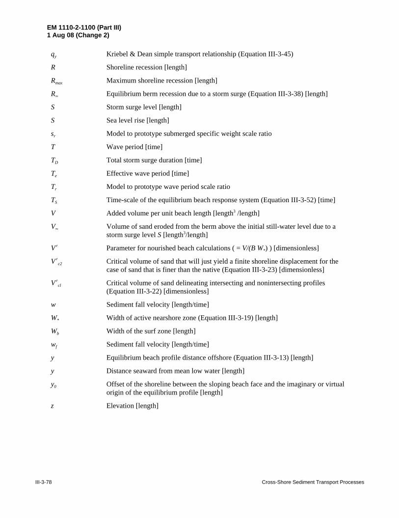
EM 1110-2-1100 (Part III)1 Aug 08 (Change 2)
III-3-78 Cross-Shore Sediment Transport Processes
qy Kriebel & Dean simple transport relationship (Equation III-3-45)
R Shoreline recession [length]
Rmax Maximum shoreline recession [length]
R4 Equilibrium berm recession due to a storm surge (Equation III-3-38) [length]
S Storm surge level [length]
S Sea level rise [length]
sr Model to prototype submerged specific weight scale ratio
T Wave period [time]
TD Total storm surge duration [time]
Te Effective wave period [time]
Tr Model to prototype wave period scale ratio
TS Time-scale of the equilibrium beach response system (Equation III-3-52) [time]
V Added volume per unit beach length [length3 /length]
V4 Volume of sand eroded from the berm above the initial still-water level due to astorm surge level S [length3/length]
VN Parameter for nourished beach calculations ( = V/(B W*) ) [dimensionless]
VNc2 Critical volume of sand that will just yield a finite shoreline displacement for thecase of sand that is finer than the native (Equation III-3-23) [dimensionless]
VNcl Critical volume of sand delineating intersecting and nonintersecting profiles(Equation III-3-22) [dimensionless]
w Sediment fall velocity [length/time]
W* Width of active nearshore zone (Equation III-3-19) [length]
Wb Width of the surf zone [length]
wf Sediment fall velocity [length/time]
y Equilibrium beach profile distance offshore (Equation III-3-13) [length]
y Distance seaward from mean low water [length]
y0 Offset of the shoreline between the sloping beach face and the imaginary or virtualorigin of the equilibrium profile [length]
z Elevation [length]

EM 1110-2-1100 (Part III)1 Aug 08 (Change 2)
Cross-Shore Sediment Transport Processes III-3-79
III-3-6. Acknowledgments
Authors of Chapter III-3, “Cross-Shore Sediment Transport Processes:”
Robert G. Dean, Ph.D., Coastal & Oceanographic Engineering, University of Florida, Gainesville, Florida.David L. Kriebel, Ph.D., Department of Ocean Engineering, United States Naval Academy, Annapolis,
Maryland.Todd L. Walton, Ph.D., Coastal and Hydraulics Laboratory, Engineer Research and Development Center,
Vicksburg, Mississippi.
Reviewers:Kevin Bodge, Ph.D., Olsen Associates, Jacksonville, Florida.James R. Houston, Ph.D., Engineer Research and Development Center, Vicksburg, Mississippi.Paul A. Work, Ph.D., School of Civil and Environmental Engineering, Georgia Institute of Technology,
Atlanta, Georgia.

Wind-Blown Sediment Transport III-4-i
Chapter 4 EM 1110-2-1100WIND-BLOWN SEDIMENT TRANSPORT (Part III)
30 April 2002
Table of Contents
Page
III-4-1. Introduction . . . . . . . . . . . . . . . . . . . . . . . . . . . . . . . . . . . . . . . . . . . . . . . . . . . . . . . . . . . . III-4-1
III-4-2. Wind Regime of U.S. Coastal Areas . . . . . . . . . . . . . . . . . . . . . . . . . . . . . . . . . . . . . . III-4-1a. Introduction . . . . . . . . . . . . . . . . . . . . . . . . . . . . . . . . . . . . . . . . . . . . . . . . . . . . . . . . . . . III-4-1b. Sample wind environments . . . . . . . . . . . . . . . . . . . . . . . . . . . . . . . . . . . . . . . . . . . . . . . III-4-1c. Wind direction . . . . . . . . . . . . . . . . . . . . . . . . . . . . . . . . . . . . . . . . . . . . . . . . . . . . . . . . . III-4-1
(1) Basic concepts . . . . . . . . . . . . . . . . . . . . . . . . . . . . . . . . . . . . . . . . . . . . . . . . . . . . . . III-4-2(2) Measurement of wind speed and direction . . . . . . . . . . . . . . . . . . . . . . . . . . . . . . . III-4-12(3) Effects of vegetation, dunes, and buildings . . . . . . . . . . . . . . . . . . . . . . . . . . . . . . III-4-15
III-4-3. Transport Rates . . . . . . . . . . . . . . . . . . . . . . . . . . . . . . . . . . . . . . . . . . . . . . . . . . . . . . . III-4-16a. Processes of sand transport by wind . . . . . . . . . . . . . . . . . . . . . . . . . . . . . . . . . . . . . . . III-4-16b. Sand transport rate prediction formulas . . . . . . . . . . . . . . . . . . . . . . . . . . . . . . . . . . . . III-4-18c. Initiation of sand transport . . . . . . . . . . . . . . . . . . . . . . . . . . . . . . . . . . . . . . . . . . . . . . III-4-21
III-4-4. Procedures for Calculating Wind-Blown Sand Transport . . . . . . . . . . . . . . . . . III-4-21
III-4-5. Wind-Blown Sand Transport and Coastal Dunes . . . . . . . . . . . . . . . . . . . . . . . . . III-4-39a. Dunes and dune processes . . . . . . . . . . . . . . . . . . . . . . . . . . . . . . . . . . . . . . . . . . . . . . III-4-39b. Factors affecting dune growth rates . . . . . . . . . . . . . . . . . . . . . . . . . . . . . . . . . . . . . . . III-4-51c. Dune sediment budget . . . . . . . . . . . . . . . . . . . . . . . . . . . . . . . . . . . . . . . . . . . . . . . . . . III-4-54d. Procedure to estimate dune "trapping factor" . . . . . . . . . . . . . . . . . . . . . . . . . . . . . . . III-4-55e. Continuity equation for wind transport of beach sand . . . . . . . . . . . . . . . . . . . . . . . . . III-4-59f. Limited source due to gradation armoring . . . . . . . . . . . . . . . . . . . . . . . . . . . . . . . . . . III-4-61
III-4-6. References . . . . . . . . . . . . . . . . . . . . . . . . . . . . . . . . . . . . . . . . . . . . . . . . . . . . . . . . . . . III-4-72
III-4-7. Definition of Symbols . . . . . . . . . . . . . . . . . . . . . . . . . . . . . . . . . . . . . . . . . . . . . . . . . . III-4-76
III-4-8. Acknowledgments . . . . . . . . . . . . . . . . . . . . . . . . . . . . . . . . . . . . . . . . . . . . . . . . . . . . . III-4-77

EM 1110-2-1100 (Part III)30 Apr 02
III-4-ii Wind-Blown Sediment Transport
List of Tables
Page
Table III-4-1Monthly Mean Wind Speeds Near Westhampton Beach, Long Island, NY - Based onSimultaneous Measurements at C-MAN Station ALSN6 and Offshore Buoy 44025 . . . . . . . . . . . III-4-15
Table III-4-2Predictive Capability of Sand Transport Equations (Chapman 1990) . . . . . . . . . . . . . . . . . . . . . . . III-4-19
Table III-4-3Hourly Wind Data, Westhampton Beach, Long Island, NY . . . . . . . . . . . . . . . . . . . . . . . . . . . . . . III-4-33
Table III-4-4Hourly Transport Analysis under Dry Conditions, Westhampton Beach, Long Island, NY . . . . III-4-34
Table III-4-5Hourly Transport Analysis Under Wet Conditions, Westhampton Beach, Long Island, NY . . . . . III-4-38
Table III-4-6Monthly Sand Transport at Westhampton Beach, Long Island, NY(All Data Considered) (Hsu 1994) . . . . . . . . . . . . . . . . . . . . . . . . . . . . . . . . . . . . . . . . . . . . . . . . . . III-4-41
Table III-4-7Monthly Sand Transport at Westhampton Beach, Long Island, NY(Snow Days Excluded) (Hsu 1994) . . . . . . . . . . . . . . . . . . . . . . . . . . . . . . . . . . . . . . . . . . . . . . . . . III-4-41
Table III-4-8Monthly Sand Transport at Westhampton Beach, Long Island, NY(Snow Days and Wet Days Excluded) (Hsu 1994) . . . . . . . . . . . . . . . . . . . . . . . . . . . . . . . . . . . . . III-4-41
Table III-4-9Wind Rose Data, Atlantic City, NJ(Wind Data, 1936 to 1952) . . . . . . . . . . . . . . . . . . . . . . . . . . . . . . . . . . . . . . . . . . . . . . . . . . . . . . . III-4-44
Table III-4-10Wind Rose Data Analysis, Atlantic City, NJ(Anemometer at Standard 10-m Height) . . . . . . . . . . . . . . . . . . . . . . . . . . . . . . . . . . . . . . . . . . . . . III-4-44
Table III-4-11Wind-Blown Sand Transport Analysis, Wind Rose DataAtlantic City, NJ (Wind Data, 1936 to 1952) . . . . . . . . . . . . . . . . . . . . . . . . . . . . . . . . . . . . . . . . . III-4-45
Table III-4-12Estimated Annual Dune Growth at Atlantic City, NJ . . . . . . . . . . . . . . . . . . . . . . . . . . . . . . . . . . . III-4-50
Table III-4-13Measured Dune Growth Rates (adapted from SPM 1984) . . . . . . . . . . . . . . . . . . . . . . . . . . . . . . . III-4-52

EM 1110-2-1100 (Part III)30 Apr 02
Wind-Blown Sediment Transport III-4-iii
Table III-4-14Typical Beach and Dune Sand Phi Diameters and Dune Trapping Factors Calculated fromBeach and Dune Sand Samples at Various U. S. Beaches . . . . . . . . . . . . . . . . . . . . . . . . . . . . . . . III-4-59
Table III-4-15Size Distribution, Threshold Wind Speeds, and Volumetric Transport Coefficients forBeach Sand Size Intervals, Atlantic City, NJ . . . . . . . . . . . . . . . . . . . . . . . . . . . . . . . . . . . . . . . . . . III-4-63
Table III-4-16Wind Speeds for Atlantic City Wind Rose Intervals . . . . . . . . . . . . . . . . . . . . . . . . . . . . . . . . . . . . III-4-63
Table III-4-17Transport Rates for Size Intervals at Atlantic City Wind Rose Speed Intervals . . . . . . . . . . . . . . . III-4-64
Table III-4-18Wind Transport of Size Intervals for Winds from North Weighted by Fraction of YearWind was Within Given Speed and Direction Interval . . . . . . . . . . . . . . . . . . . . . . . . . . . . . . . . . . III-4-65
Table III-4-19Summary of Transports for Eight Compass Directions . . . . . . . . . . . . . . . . . . . . . . . . . . . . . . . . . . III-4-66
Table III-4-20Computation of Dune Growth Rate . . . . . . . . . . . . . . . . . . . . . . . . . . . . . . . . . . . . . . . . . . . . . . . . . III-4-67
Table III-4-21Calculated Dune Sand Size Distribution . . . . . . . . . . . . . . . . . . . . . . . . . . . . . . . . . . . . . . . . . . . . . III-4-68
Table III-4-22Comparison of Calculated Dune Sand Size Distribution and Actual Dune SandSize Distribution . . . . . . . . . . . . . . . . . . . . . . . . . . . . . . . . . . . . . . . . . . . . . . . . . . . . . . . . . . . . . . . III-4-70
Table III-4-23Corrected Transport Rates for Size Intervals and Corrected Dune Growth Rate . . . . . . . . . . . . . . . III-4-71
EM 1110-2-1100 (Part III)30 Apr 02
III-4-iv Wind-Blown Sediment Transport
List of Figures
Page
Figure III-4-1. Air masses and fronts over the coastal areas . . . . . . . . . . . . . . . . . . . . . . . . . . . III-4-2
Figure III-4-2. Example wind regime areas (Solid circles denote example wind regimeareas. Open circles are nearby buoys used to construct wind roses) . . . . . . . . . III-4-3
Figure III-4-3. Wind roses based on hourly data nearby: (a) Newport, OR, (b) AransasPass, TX, (c) Westhampton Beach, Long Island, NY, and(d) New Buffalo, MI . . . . . . . . . . . . . . . . . . . . . . . . . . . . . . . . . . . . . . . . . . . . . . III-4-4
Figure III-4-4. Example logarithmic wind profile at Isles Dernieres, LA (adoptedfrom Hsu and Blanchard 1991) . . . . . . . . . . . . . . . . . . . . . . . . . . . . . . . . . . . . . . III-4-6
Figure III-4-5. Aerodynamic roughness element lengths Z0 and relationship betweenshear velocity u* and wind speed at the 2-m height U2m in coastalenvironments (adopted from Hsu (1977)) . . . . . . . . . . . . . . . . . . . . . . . . . . . . III-4-10
Figure III-4-6. Variation of Usea with Uland. (Hsu 1986) . . . . . . . . . . . . . . . . . . . . . . . . . . . . . . III-4-14
Figure III-4-7. Temperature correction factor RT as a function of air-sea temperaturedifference (Resio and Vincent 1977) . . . . . . . . . . . . . . . . . . . . . . . . . . . . . . . . III-4-14
Figure III-4-8. Wind field in the vicinity of a coastal sand dune (q is the local resultantmean velocity and v is the reference velocity in the uniform stream above the dune) (Hsu 1988) . . . . . . . . . . . . . . . . . . . . . . . . . . . . . . . . . . . . . . . III-4-16
Figure III-4-9. Wind-blown sand transport coefficient as a function of mean sand-grain diameter (adopted from Hsu (1977)) . . . . . . . . . . . . . . . . . . . . . . . . . . . . III-4-20
Figure III-4-10. Westhampton Beach, Long Island, NY (Hsu 1994) . . . . . . . . . . . . . . . . . . . . . III-4-22
Figure III-4-11. Threshold (critical) wind speed as a function of median sand-graindiameter and the anemometer height at which wind speed is measured . . . . . . III-4-27
Figure III-4-12. Mass transport rate coefficient K* as a function of median sand-graindiameter and the anemometer height at which wind speed is measured . . . . . . III-4-29
Figure III-4-13. Volume transport rate coefficient K*V as a function of median sand-grain
diameter and the anemometer height at which wind speed is measured(assumes sediment density = 2.65 gm/cm3 and porosity = 0.4) . . . . . . . . . . . . III-4-31
Figure III-4-14. Wet sand transport rate coefficient as a function of median sand-graindiameter and the anemometer height at which wind speed is measured . . . . . . III-4-36
Figure III-4-15. Wind-blown sand transport rose at Westhampton Beach, Long Island, NY,for 1989 (Hsu 1994) . . . . . . . . . . . . . . . . . . . . . . . . . . . . . . . . . . . . . . . . . . . . . III-4-40

EM 1110-2-1100 (Part III)30 Apr 02
Wind-Blown Sediment Transport III-4-v
Figure III-4-16. Wind rose for Atlantic City, NJ (data from 1936 to 1952) . . . . . . . . . . . . . . . . III-4-43
Figure III-4-17. Net sand transport at an angle α with the wind direction . . . . . . . . . . . . . . . . . III-4-47
Figure III-4-18. Shoreline orientation with respect to compass directions atAtlantic City, NJ . . . . . . . . . . . . . . . . . . . . . . . . . . . . . . . . . . . . . . . . . . . . . . . . III-4-48
Figure III-4-19. Sand transport efficiency for winds blowing from dunes toward beachas a function of the angle between wind direction and shoreline . . . . . . . . . . . III-4-49
Figure III-4-20. Definition of angle ß, between wind and shoreline . . . . . . . . . . . . . . . . . . . . . III-4-49
Figure III-4-21. Schematic views of sorted sand deposits: (a) well-sorted (poorly graded);(b) poorly sorted (well-graded); (c) poorly sorted after fines have beenremoved by wind erosion . . . . . . . . . . . . . . . . . . . . . . . . . . . . . . . . . . . . . . . . . III-4-53
Figure III-4-22. Definition of terms, dune sediment budget . . . . . . . . . . . . . . . . . . . . . . . . . . . . III-4-54
Figure III-4-23. Dune sand trapping factor Tf . . . . . . . . . . . . . . . . . . . . . . . . . . . . . . . . . . . . . . . III-4-56
Figure III-4-24. Sand conservation equations for a beach showing deflation area,equilibrium area, and deposition area . . . . . . . . . . . . . . . . . . . . . . . . . . . . . . . . III-4-60
Figure III-4-25. Beach and dune and size gradations for Atlantic City, NJ . . . . . . . . . . . . . . . . III-4-62
Figure III-4-26. Actual and calculated dune sand size gradation at Atlantic City, NJ . . . . . . . . III-4-69
Figure III-4-27. Comparison of actual dune sand size gradation with corrected,calculated gradation . . . . . . . . . . . . . . . . . . . . . . . . . . . . . . . . . . . . . . . . . . . . . III-4-71

EM 1110-2-1100 (Part III)30 Apr 02
Wind-Blown Sediment Transport III-4-1
Chapter III-4Wind-Blown Sediment Transport
III-4-1. Introduction
From an engineering perspective, the transport of sand by wind is often an important component in the coastalsediment budget. Wind transport can lead to the removal of sand or its redistribution within the littoral zone.Onshore winds carry sand from the beach and deposit it in backshore marshes, in developed backshore areas,or in natural or man-made dunes. Offshore winds carry sand from the beach into the sea or lake. In someareas, wind-blown sand is a nuisance and must be controlled. In other areas, the natural growth of protectivedunes is limited by the amount of sand transported to them by wind. Wind transport of sand is a continual,natural process that is often significant in bringing about beach changes. It is important to be able toquantitatively predict how much sand will be transported by wind at a given coastal site, the direction inwhich that sand will be transported, and where it will be deposited. This chapter discusses wind transportprediction in coastal areas by describing the driving force (the wind) and the transport mechanisms. Theoverall wind regime of U.S. coastal areas, modifications to the wind field brought about by its proximity tothe ground (the atmospheric boundary layer), initiation of sediment motion under wind, processes involvedin sand transport by wind, and the quantitative prediction of transport rates are described.
III-4-2. Wind Regime of U.S. Coastal Areas
a. Introduction. In the Northern Hemisphere, between the equator and latitude 30E N, winds generallyblow from the east (the trade winds), while between 30E N and 60E N, winds blow generally from the west(the prevailing westerlies). From autumn to spring, however, cold fronts frequently pass over the UnitedStates. During these events the normal wind regime is different. Ahead of these fronts, winds are generallysoutherly, while behind the fronts, winds are northerly. Southerly winds ahead of the front transport warmertropical air northward while behind the front, northerly winds transport cold polar air southward (seeFigure III-4-1).
b. Example wind environments. Four coastal areas are considered herein as example wind environments(see Figure III-4-2). The sites are: Newport, OR; Aransas Pass, TX; Westhampton Beach, NY; and NewBuffalo, MI on Lake Michigan. The four sites represent a broad range of geographical parameters. Windroses for each area are given in Figure III-4-3. Since sand transport generally occurs for wind speeds greaterthan about 5-m/s (approximately 10 knots), the 5 m/s wind speed is used to separate the winds into tworegimes.
c. Wind direction. Winds at Newport, OR, have a major north-south component because the CascadeRange immediately behind the shoreline has a north-south orientation and because of the north-southorientation of the shoreline. Occasionally, winds may blow from land toward the sea. In Port Aransas, TX,winds come mostly from the southeast because of the influence of Bermuda high pressure systems. AtWesthampton Beach, NY, winds blow mainly from the southwest around through the northwest. At NewBuffalo, MI, in the Lake Michigan region, winds blow generally in the north-south direction because of thewest-to-east passage of fronts. These wind conditions are in general agreement with the air mass and coldfront influences shown in Figure III-4-1.

EM 1110-2-1100 (Part III)30 Apr 02
III-4-2 Wind-Blown Sediment Transport
Figure III-4-1. Air masses and fronts over the coastal areas
u('
τρa
(III-4-1)
(1) Basic concepts.
(a) Wind velocity and the vertical gradient of wind speed near the ground are important factors indetermining how much sediment will be transported by wind. In addition, sediment characteristics such assize, size distribution, packing, and moisture content play important roles. The vertical gradient of windspeed results in shearing forces within the air and eventually on the ground surface. When vegetation ispresent, sheer can be transferred into the uppermost soil layers. The steeper the gradient, the greater the shearstress. The velocity gradient is significantly influenced by local topography, vegetation, and land use. Thesefactors contribute to the “roughness” of the ground surface. In the case of wind transport in coastal areas,local perturbations in the wind field may also be important in determining the eventual erosion and depositionpatterns of wind-blown sand.
(b) The vertical distribution of wind speed - the velocity profile - generally follows a logarithmicdistribution. An important parameter in this representation is the shear velocity defined by

EM 1110-2-1100 (Part III)30 Apr 02
Wind-Blown Sediment Transport III-4-3
Figure III-4-2. Example wind regime areas (Solid circles denote example wind regime areas. Open circlesare nearby buoys used to construct wind roses)
Uz 'u(
κln
Zo % ZZo
(III-4-2)
Uz .u(
κln Z
Zo(III-4-3)
in which u* = the shear or friction velocity, τ = the boundary shear stress (force per unit surface area), and ρa =the density of the air. The logarithmic distribution of wind velocity is given by
in which Uz = the average wind speed as a function of height above ground level, u* = the shear velocity, Z =the height above ground level, Zo = the height of a roughness element characterizing the surface over whichthe wind is blowing, and κ = von Karman's constant (κ = 0.4). Wind speed measurements are usuallyaveraged over a period of several minutes to smooth out fluctuations due to gusts. Averaging time can varydepending on how the measurements are made. If readings are taken from an anemometer dial rather thanfrom a recording, the observer may visually average the speed by observing the needle over a period ofseveral minutes. Wind speeds are occasionally reported as the fastest mile of wind speed where the averagingtime is the time it would take the wind to travel the distance of 1 mile; thus, the averaging time for a 60-mphwind would be 1 min; the averaging time for a 30-mph wind would be 2 min, etc.
(c) Since the height of a roughness element Zo is usually small compared with Z, Equation 4-2 can beapproximated by
or

EM 1110-2-1100 (Part III)30 Apr 02
III-4-4 Wind-Blown Sediment Transport
Figure III-4-3. Wind roses based on hourly data nearby: (a) Newport, OR, (b) Aransas Pass, TX,(c) Westhampton Beach, Long Island, NY, and (d) New Buffalo, MI
BOUY #46010
LEGEND
--=:] <5m/s 1 >5m/s (10kts) (10kts)
BOUY
LEGEND
--=:] <5m/s 1 >5m/s (10kts) (10kts)
N
(o)
s
N
(c)
s
BOUY #42008
LEGEND
--=:] <5m/s 1 >5m/s (10kts) (10kts)
BOUY #45007
LEGEND
--=:] <5m/s 1 >5m/s (10kts) (10kts)
N
(b)
s
N
(d)
s

EM 1110-2-1100 (Part III)30 Apr 02
Wind-Blown Sediment Transport III-4-5
ln Z ' ln Zo %κu(
Uz
Y ' ao % a1 X
ao ' ln Zo or, Zo ' e ao
a1 'κu(
or, u('
κa1
Cz 'u(
Uz
2
(III-4-4)
ln Z1 ' ln Zo %κu(
Uz1 (III-4-5)
ln Z2 ' ln Zo %κu(
Uz2 (III-4-6)
which is of the form
where Y = ln Z and
and
(d) A logarithmic velocity distribution as fit by linear regression techniques is given in Figure III-4-4 forIsle Dernieres, LA.
(e) The concept of a drag coefficient is sometimes used in wind transport calculations, where the dragcoefficient is defined as
in which Cz = the drag coefficient at height Z. Often Cz is considered a constant for a given Z; however,computations by Hsu and Blanchard (1991) for C10 showed a variation of from 0.5 × 10⁻³ to 5.0 × 10⁻³, anorder of magnitude. In fact, Cz varies with season and wind direction and cannot be considered constant. Itis evident that the roughness characteristics of the fetch over which the wind blows depend on wind direction,particularly in coastal regions where onshore and offshore winds experience significantly different fetches.Onshore winds usually experience less friction than offshore winds because of the relative smoothness of thewater surface when compared with the rougher land surface. On the other hand, shear stresses on the beachdue to onshore winds will be greater than shear stresses due to offshore winds of the same speed.
(f) Because the appropriate height of a roughness element is not known a priori, it must be found by thesimultaneous solution of Equation 4-2 applied at two heights above the ground. However, if Zo is small, andthe wind speed is not measured very close to the ground (well outside of the roughness elements), Equation 4-3 can be used to estimate the wind speed distribution without first finding Zo. Equation 4-3 can be appliedat two heights, Z1 and Z2 so that
and

EM 1110-2-1100 (Part III)30 Apr 02
III-4-6 Wind-Blown Sediment Transport
Figure III-4-4. Example logarithmic wind profile at Isles Dernieres, LA (adoptedfrom Hsu and Blanchard (1991))
u('
κ (Uz2 & Uz1)
lnZ2
Z1
(III-4-7)
where Z1 is below Z2 so that UZ1 is less than UZ2.
(g) Eliminating Zo from Equations 4-5 and 4-6 gives
(h) Consequently, the shear velocity u* can be determined from Equation 4-7 without first finding Zo bymeasuring the wind velocity at two elevations. For wind transport studies, wind velocity sensors used todetermine u* should be spaced vertically as far apart as practical, say a minimum of 3 to 4 m, but preferablymore.

EM 1110-2-1100 (Part III)30 Apr 02
Wind-Blown Sediment Transport III-4-7
11.3 'u(
0.4ln
10 % Zo
Zo
9.36 'u(
0.4ln
4 % Zo
Zo
9.36 (0.4)
ln4 % Zo
Zo
'11.3 (0.4)
ln10 % Zo
Zo
ln10 % Zo
Zo
' 1.207 ln4 % Zo
Zo
ln (Zo % 10) & lnZo ' 1.207 ln(Zo % 4) & lnZo
ln (10 % Zo) ' 1.207ln(4 % Zo) & 0.207lnZo
EXAMPLE PROBLEM III-4-1
Find:The shear velocity u* and the height of a characteristic roughness element Zo. What is the
magnitude of the shear stress acting on the ground surface?
Given:Wind speed is measured at two elevations above the ground. At 10 m height, the average wind
speed is 11.3 m/s; at 4 m, it is 9.36 m/s.
Solution:The velocity distribution is logarithmic as given by Equation 4-2. Since there are two unknowns,
Zo and u*, the equation must be solved at the two elevations. Substituting into the equation with κ =0.4
and
Solving for each equation for u* and equating
or
Assuming that Zo is small with respect to the height at which the wind speeds are measured, a firstapproximation to Zo can be obtained,
(Sheet 1 of 3)

EM 1110-2-1100 (Part III)30 Apr 02
III-4-8 Wind-Blown Sediment Transport
ln(10) ' 1.207 ln(4) & 0.207 lnZo
2.303 ' 1.673 & 0.207 lnZo
lnZo ' &3.042
Zo ' 0.0477 m
ln(10 % 0.0477) ' 1.207ln(4 % 0.0477) & 0.207lnZo
Zo ' 0.05 m
u('
Uzκ
lnZ % Zo
Zo
u('
(11.3) (0.4)
ln 10 % 0.050.05
' 0.852 m/s
Uz 'u(
0.4ln Z
Zo
11.3 'u(
0.4ln 10
Zo
Example Problem III-4-1 (Continued)
A second improved approximation can be found by substituting Zo = 0.0477 into,
Solving for Zo
Then, substituting back into one of the wind speed equations
for the wind speed observation at 10 m
The assumption that Zo is small with respect to the height at which wind speeds are measured couldhave been made at the outset by using Equation 4-3. Then
and
(Sheet 2 of 3)

EM 1110-2-1100 (Part III)30 Apr 02
Wind-Blown Sediment Transport III-4-9
9.36 'u(
0.4ln 4
Zo
(11.3)(0.4) ' u(
ln(10) & lnZo
(9.36)(0.4) ' u(
ln(4) & lnZo
0.776 ' u(
ln 104
u(' 0.847 m/s
Z0 ' 0.048 m
u('
τρa
τ ' ρa u(
2
τ ' 0.00122(85.2)2 ' 8.86 dynes/cm2
Example Problem III-4-1 (Concluded)with
or
and
Subtracting
On substituting this value for u* back into one of the above equations and solving for Z0 gives
These are the same as the first approximations found above.
The shear stress can be found from Equation 4-1, the definition of u*
or
where ρa = 0.00122 gm/cm3 and u* = 0.852 m/sec. Substituting
The reader may wish to verify the shear velocity and characteristic roughness element height for thewind speed observation at Isle Dernieres given in Figure III-4-4.
(Sheet 3 of 3)

EM 1110-2-1100 (Part III)30 Apr 02
III-4-10 Wind-Blown Sediment Transport
u(' 0.044 U2m (III-4-8)
Figure III-4-5. Aerodynamic roughness element lengths Z0 and relationship between shear velocity u* andwind speed at the 2-m height U2m in coastal environments (adopted from Hsu (1977))
(i) In most sand transport studies, two-level or multilevel wind velocity measurements are rarelyavailable and the wind speed climatology must be measured at two or more levels to establish u*. Based onmeasurements at six beaches, Hsu (1977) established a relationship for u* in terms of U2m, the wind speed atthe 2-m height (see Figure III-4-5). His relationship for the dry beach area is given by
in which U2m = the average wind speed at the 2-m height. Equations for u* on tidal flats, dunes, etc. are alsogiven by Hsu (1977) (see Figure III-4-5). Note that the coefficient in this equation depends critically on theheight of a roughness element so that Equation 4-8 is valid only for beaches with roughness conditions similarto those for which the equation was developed.

EM 1110-2-1100 (Part III)30 Apr 02
Wind-Blown Sediment Transport III-4-11
C10m 'u(
U10m
2
C10m '0.85211.3
2' 0.00568
U2m '(0.852)
(0.4)ln 2 % 0.05
0.05
U2m ' 7.91 m/s
C2m '0.8527.91
2' 0.0116
u(' 0.044U2m
u(' 0.044(7.91) ' 0.348 m/s
EXAMPLE PROBLEM III-4-2
Find:The drag coefficient at the 10-m, 4-m, and 2-m heights using the shear velocity calculated in the
preceding problem, then estimate the shear velocity using the wind speed determined for the 2-m height.Compare the shear velocity with the value determined in the preceding example problem.
Given:The wind speed measurements from the previous example problem.
Solution:The definition of the drag coefficient is given by Equation 4-4. Thus, for the 10-m height,
For the 4-m height C4m = (0.852/9.36)2 = 0.00829. The wind speed at the 2-m height must be found fromEquation 4-2 (or Equation 4-3 if the roughness element height can be assumed small). Thus,
and
Using this wind speed at the 2-m height to estimate the shear velocity u* in Equation 4-8 gives
This result is significantly lower than the u* = 0.852 value found from the wind speed distributionbecause the example wind speed distribution is somewhat unusual for a beach. The characteristicroughness length for the example is larger than what is typically found on beaches. A value of Zo typicalfor beaches is 0.000225 m (0.0225 cm); however, based on measurements by Hsu (1977), Zo can bemuch larger in the lee of dune areas. See Figure III-4-5 for some typical values of Zo in various coastalenvironments.

EM 1110-2-1100 (Part III)30 Apr 02
III-4-12 Wind-Blown Sediment Transport
Usea
Uland
'Hsea CD, land
Hland CD, sea
12 (III-4-9)
Usea ' A % BUland (III-4-10)
(2) Measurement of wind speed and direction.
(a) Wind speed is measured with an anemometer. Two types of anemometers are typically used, cup-type or propeller-type anemometers. Wind direction is measured using a vane that indicates the directionfrom which the wind is blowing. When wind speed measurements are made with a cup-type anemometer,a separate vane is needed. Propeller-type anemometers have a built-in vane that keeps the propeller directedinto the wind. Wind speed measurements are usually obtained at or corrected to a standard anemometerheight of 10 m above ground level, although anemometers may be mounted at other heights. The wind recordfrom an anemometer depends significantly on the physical conditions of the surrounding terrain. Thesurrounding terrain determines the boundary roughness and thus the rate at which wind speed increases withheight above the ground. Consequently, physical conditions characterizing the surrounding fetches determinethe wind environment at a site. At coastal sites, the fetch seaward of the beach is over water and is generallycharacterized by relatively low roughness. The fetch landward of the beach can vary significantly from siteto site since it depends on the type of vegetation, terrain, etc.
(b) Differences exist between onshore and offshore wind speeds due to differences in friction conditionsover the fetch. The differences are most marked in the observed wind speeds (see Hsu (1988)). Hsu (1986)derived an equation to estimate the difference in overwater and overland wind speeds. The ratio of windspeed overwater to the wind speed overland is given by
where
Usea and Uland = the wind speed over sea and land, respectively
Hsea and Hland = the height of the planetary boundary layer over the sea and land
CD,sea and CD,land = the drag coefficients over sea and land
(c) Equation 4-9 should apply for both onshore and offshore winds assuming that the geostrophic windabove the boundary layer does not change appreciably. For a given climatological area, the parameters onthe right side of Equation 4-9 are generally known. Holzworth (1972) and SethuRaman and Raynor (1980)found Hsea = 620 m, Hland = 1014 m, CD,sea 0.0017, and CD,land = 0.0083, leading to Usea/Uland = 1.7 for this area.CD,sea and CD,land were measured at the 8-m level.
(d) If the direction between either onshore near-surface winds or offshore near-surface winds is within45 deg of shore-normal, Equation 4-9 will be valid regardless of whether the wind blows from land to sea orvice versa (Hsu (1988), pp 184-186). Equation 4-9 may, therefore, be applicable to weather systems suchas land breezes, sea breezes, hurricanes near landfall, and other synoptic-scale phenomena such as cyclones(low pressure cells), anti-cyclones (high pressure cells), and monsoons. This is not the case for the passageof frontal systems and squall lines, however, since their winds do not usually blow within 45 deg of shore-normal. Typically, winds associated with the passage of fronts and squall lines do not persist for long periodsof time.
(e) An empirical relationship between overland wind speed and overwater wind speed can be estimatedfrom measured wind speeds at land and water sites by

EM 1110-2-1100 (Part III)30 Apr 02
Wind-Blown Sediment Transport III-4-13
Usea ' 1.85 (m/s) % 1.2 Uland (III-4-11)
Usea ' 1.62 (m/s) % 1.17 Uland (III-4-12)
U )
10m ' RT U10m (III-4-13)
RT ' 1 & 0.06878*Ta & Ts*0.3811 sign(Ta & Ts) (III-4-14)
where A and B are empirical constants.
(f) If the air-water temperature difference is small, say less than 5 EC, and if the aggregate windestimation error at airports is less than 10 percent (Wieringa 1980), then an estimate is given by Liu, Schwab,and Bennett (1984) as
where Usea and Uland are measured in m/s.
(g) Based on many pairs of measurements of overland and overwater wind speeds, the Usea was correlatedwith Uland for synoptic-scale weather systems (Hsu 1981; Powell 1982). Wind speeds used by Hsu (1981)were less than 18 m/s while Powell's (1982) data included hurricane-force wind speeds obtained duringHurricane Frederic in Alabama in 1979. The correlation between Usea and Uland is shown in Figure III-4-6.The best-fit equation by linear regression methods is given by
(h) Equation 4-11 is also plotted in Figure III-4-6. The difference between Equations 4-11 and 4-12 isnot significant even though the correlation on which Equation 4-12 is based did not consider air-seatemperature differences. Equation 4-12 is recommended for use in coastal wind-blown sand transport studieswhere the air water temperature difference is small (|Ta - Ts| < 5 EC).
(i) For air-sea temperature differences exceeding 5 EC, a correction can be applied. A temperaturecorrection applied to wind speed as given by Resio and Vincent (1977) is
where UN10m is the wind speed corrected for the air-sea temperature difference and RT is the correction factorapplied to the overwater wind speed at the 10-m height. The correction factor RT is shown in Figure III-4-7and given by the equation
where Ta = the air temperature in degrees Celsius and Ts = the sea temperature in degrees Celsius.
(j) For wind-blown sand transport studies, wind measurement stations should be close to the study siteand preferably on the beach. Land-based wind measurements at airports are generally not useful indicatorsof nearshore wind conditions and should not be used for coastal sand transport studies. Unfortunately, windmeasurements are often not available near coastal study sites and data from nearby Coastal Marine AutomatedNetwork (C-MAN) and offshore meteorological buoys must be used. Table III-4-1 compares windmeasurements at a C-MAN station (ALSN6), at an offshore buoy 44025, and at Islip Airport on central LongIsland. (Wind speeds have been corrected to the standard 10-m elevation using a power-law relation. Thiscorrection is discussed below.) Wind speed measurements at Islip Airport are consistently lower thanmeasurements at the coast. On average, U44025/UIslip = 1.6, which is consistent with the Usea/Uland foundearlier for the New York-Massachusetts area (Holzworth 1972, SethuRaman and Raynor 1980). Also,measurements at the offshore buoy are more variable than those at the C-MAN station, making the C-MANstation data preferable in this case.

EM 1110-2-1100 (Part III)30 Apr 02
III-4-14 Wind-Blown Sediment Transport
Figure III-4-6. Variation of Usea with Uland. (Hsu 1986)
Figure III-4-7. Temperature correction factor RT as a function of air-sea temperaturedifference (Resio and Vincent 1977)

EM 1110-2-1100 (Part III)30 Apr 02
Wind-Blown Sediment Transport III-4-15
Table III-4-1Monthly Mean Wind Speeds Near Westhampton Beach, Long Island NY - Based on Simultaneous Measurements atC-MAN Station ALSN6 and Offshore Buoy 44025
Wind Speeds in meters/sec
YEAR MONTH
C-MAN BUOY C-MAN BUOY ISLIP
ALSN6 44025 ALSN6 44025 AIRPORT
@4.9 m @ 4.9 m @ 10 m @ 10 m @ 10 m
1991 May 7.30 4.70 6.20 5.00 2.60
Jun 6.70 5.40 5.70 5.80 2.90
Jul 6.00 4.70 5.10 5.00 2.40
Aug 6.80 5.00 5.80 5.40 2.80
Sep 6.60 5.80 5.60 6.20 3.80
Oct 7.60 6.30 6.50 6.70 4.50
1992 Nov 7.70 7.10 6.50 7.60 4.60
Dec 8.80 7.90 7.50 8.50 4.70
Jan 8.10 N/A 6.90 N/A 4.70
Feb 8.70 7.30 7.40 7.80 5.10
Mar 9.00 7.30 7.70 7.80 5.30
Apr 7.00 5.40 6.00 5.80 4.50
May 6.80 5.10 5.80 5.50 4.60
Jun 7.10 4.80 6.00 5.10 4.70
AVG = 7.44 5.91 6.34 6.32 4.09
STD DEV = 0.91 1.14 0.79 1.22 0.99
(k) Wind speeds are often adjusted to a standard anemometer height by using a power-law relation. Thestandard anemometer height is usually 10 m above the ground. The power-law adjustment equation is givenby
(III-4-15)UZR ' UZMZR
ZM
n
in which ZM = the anemometer height, ZR = the reference height (usually 10 m), UZM = the wind speed at theanemometer height, UZR = the wind speed at the reference height, and n = an empirically determinedexponent, ranging from 1/11 to 1/7. The following example details the calculation of this exponent as wellas wind speed correction factors for air sea temperature differences.
(3) Effects of vegetation, dunes, and buildings.
(a) Air flow over a flat beach differs from air flow over dunes. There are at least three distinct windtransport zones resulting from the presence of dunes on the backbeach (Hsu 1988). Dunes produce both astagnation zone on their windward side and a wake zone on their leeward side within which wind patternsare disturbed and no longer exhibit the typical logarithmic distribution with height above the ground. Windblowing offshore results in a stagnation zone landward of the dune that extends landward approximately twoto four times the height of the dune. In this zone, wind speeds are lower than the free stream wind speed(region of underspeed); in fact, near the ground they may even blow in the direction opposite to that of the

EM 1110-2-1100 (Part III)30 Apr 02
III-4-16 Wind-Blown Sediment Transport
Figure III-4-8. Wind field in the vicinity of a coastal sand dune (q is the local resultantmean velocity and v is the reference velocity in the uniform stream above the dune)(Hsu 1988)
free stream. A wake region (cavity) may extend 10 dune heights seaward of the dune. Within the wakecavity, wind speeds are also reduced and may reverse direction near ground level. Over the dune crest, windspeeds are higher than the free stream speed because the streamlines are compressed and the flow isaccelerated (region of overspeed) (see Figure III-4-8).
(b) Buildings and vegetation also locally modify the air flow. Generally, buildings will produce a wakein their lee. Air flow patterns near buildings will be complex, will depend on the specific building geometry,and on the presence of any surrounding buildings. Generalized air flow patterns cannot be established forthe numerous building/construction configurations encountered in practice. The effect of vegetation dependson the type of vegetation, its location relative to any dunes, and how far it projects into the near-groundboundary layer. Trees usually have more effect on wind patterns than do shrubs or grasses but, dependingon their location, may be less significant than shorter vegetation in affecting sand transport rates and sedimentdeposition patterns. Most sand transport takes place within a few centimeters of the ground and anything thatmodifies the air flow in this region will have some effect.
III-4-3. Transport Rates
a. Processes of sand transport by wind.
(1) The processes involved in transporting sand by wind are summarized by Raudkivi (1976). Sandgrains move by bouncing along the surface, a process termed saltation, and by surface creep. Sand grains,

EM 1110-2-1100 (Part III)30 Apr 02
Wind-Blown Sediment Transport III-4-17
RT ' 1 & 0.06878*15 & 5*0.3811 (%) ' 0.8346
U10m ' 0.8346(11.3) ' 9.43 m/s
Uz 'u(
κln
Z % Zo
Zo
9.43 'u(
0.4ln 10 % 0.05
0.05
u(' 0.7113 m/s
U8m '0.7113
0.4ln 8 % 0.05
0.05' 9.036 m/s
U10m
U8m
'108
n 9.439.036
' (1.25)n
n 'ln (1.0436)
ln(1.25)' 0.1913 '
15.23
EXAMPLE PROBLEM III-4-3
Find:Determine the overwater wind speed and correct the wind speed due to the air-sea temperature
difference. Estimate the exponent in Equation 4-15 using the overwater wind speeds.
Given:The winds given in Example Problem III-4-1 measured over land on a day when the air
temperature is 15 EC and the water temperature is 5 EC.
Solution:The air-sea temperature difference is (15E-5E) = 10 EC and the correction RT is given by
Equation 4-14
This correction is applied to the wind speed at the 10-m height. Therefore, from ExampleProblem III-4-1, U10m = 11.3 m/s and the corrected 10-m wind speed is
Assuming that the height of the roughness elements are Zo = 0.05 as found in Example Problem III-4-1, the shear velocity can be found from Equation 4-2
The wind speed at the 8-m height is then calculated as
Using these two wind speeds to estimate the exponent in Equation 4-15

EM 1110-2-1100 (Part III)30 Apr 02
III-4-18 Wind-Blown Sediment Transport
once dislodged, are carried up into the moving air by turbulence; they acquire energy from the moving air,and they settle through the air column due to their weight and impact on the ground. The saltating grainsimpact on the ground surface at a flat angle and transmit a portion of their energy to the grains on the ground.Some of the grains on the surface are dislodged and are carried upward into the flow where they continue theprocess of saltation; others are moved forward on the surface by the horizontal momentum of the impacting,saltating grains. This latter forward movement of sand on the ground surface is termed surface creep.Saltating grains are capable of moving much larger surface grains by surface creep due to their impact. Onbeaches, saltation is the more important of the two processes.
(2) The presence of sand in the air column near ground level also leads to a reduction in the wind speednear the ground and a modification of the wind speed distribution.
(3) Because saltating sand grains impact the ground surface at a relatively flat angle which ranges fromabout 10 to 16 deg with the horizontal, there is a tendency for small depressions in the ground surface to leadto the formation of sand ripples. Saltating sand grains have a greater tendency to impact the back face of asmall depression because of the flat angle of incidence. This preferential movement on the back face of thedepression moves sand up the back face to form a mound or ripple. Once small ripples are established theymay grow until they reach a limiting height which is determined by the prevailing wind speed.
(4) On beaches, the most important sand features frequently present are sand dunes. Dunes are muchlarger than the sand features described above. They are large enough to significantly alter wind patterns andto shelter the area on their leeward side. Once established, dunes cause wind pattern changes which lead todune growth.
b. Sand transport rate prediction formulas.
(1) Many equations have been proposed to predict sand transport by wind; e.g., see Horikawa (1988) andSarre (1988). Several example sand transport equations follow:
(O’Brien and Rindlaub 1936)G ' 0.036 U5ft3
in which G = the dry weight transport rate in pounds per foot per day and U5ft = the wind speed at the 5-ftelevation in feet per second (U5ft > 13.4 feet per second);
(Bagnold 1941)q ' BBagnoldρa
gDd
u(
3
in which q = the mass transport rate in gm/cm-s, BBagnold = a coefficient, ρa = the mass density of the air =0.001226 gm/cm3, d = a standard grain size = 0.25 mm, D = grain size in mm, and u* = the shear velocity incm/sec;
(Zingg 1953)q ' ZZinggρa
gDd
34 u
(
3
in which ZZingg = a coefficient, and q, D, d, ρa, and u* are as in the previous expression.
(2) Chapman (1990) provides an evaluation of these and several other equations. The predictivecapability of the seven equations investigated by Chapman (1990), as gauged by the coefficient ofdetermination, ranged from r2 = 0.63 to r2 = 0.87 (see Table III-4-2).

EM 1110-2-1100 (Part III)30 Apr 02
Wind-Blown Sediment Transport III-4-19
q ' Ku(
gD
3
(III-4-16)
ln K ' &9.63 % 4.91D (III-4-17a)
K ' e &9.63 % 4.91D (III-4-17b)
Table III-4-2Predictive Capability of Sand Transport Equations (Chapman 1990)
Equation Value of r2
Bagnold (1941) 0.63
Horikawa & Shen (1960) 0.84
Hsu (1973) 0.87
Kadib (1964) 0.65
O'Brien & Rindlaub (1936) 0.80
Williams (1964) 0.80
Zingg (1953) 0.78
(3) In Chapman's evaluation, Hsu's (1986) equation, which like Bagnold's (1941) is based onconsiderations of the turbulent kinetic energy relationship, had an r2 = 0.87. Hsu's equation is given by
where
q = sand transport rate in gm/cm-s
u* = shear velocity
g = acceleration of gravity
D = mean sand grain diameter
K = dimensional eolian sand transport coefficient
(4) The term in square brackets in Equation 4-16 is a dimensionless Froude number, which can becomputed using any consistent units. The dimensions of K are the same as those of q; in this case, grams percentimeter per second. Values of K as a function of sand grain diameter can be obtained from Figure III-4-9.A regression equation (r2 = 0.87) fitted to both laboratory and field data is given by
or
where D is in millimeters and K in grams per centimeter per second, which plots as a straight line on semi-logarithmic graph paper (see Figure III-4-9).
(5) Equations 4-16 and 4-17a can be used to estimate sand transport rates for given wind speeds andmean sand-grain diameters within the range of empirical observations from which the equations weredeveloped. Equation 4-17a is based on the data in Figure III-4-9, which include transport data for mean sandgrain diameters up to 1.0 mm; consequently, the equations should not be used to estimate transport on beacheswith mean grain diameters greater than about 1.0 mm.

EM 1110-2-1100 (Part III)30 Apr 02
III-4-20 Wind-Blown Sediment Transport
Figure III-4-9. Wind-blown sand transport coefficient as a function of mean sand-grain diameter (adoptedfrom Hsu (1977)
.04
• Bognold, 1936
.02 0 O'Brien and Rindoub, 1936
& Zingg, 1952
.01 ... Kawamura, 1 951 . 008 • Horikawa, 1960 . 006
D .004
Belly, 1962
~ *' Kodib, 1963 u Q)
* Kodib, 1965 CJ)
I .002 E >f. Svosek and u
" Terwindt, 1974 E "' D .001 'L .0008 ~
D c .0006 Q) o., () ~ .0004 ~
Q)
* 0 u
~ L • 0 .0002 Q_ CJ)
c & 0 L ~
I .0001 v • c .00008 0
*' & (f)
.00006 c 0
£.n, K~-9.63+4.91 0 0 .00004 w
0 .1 .2 .3 .4 .5 .6 .7 .8 .9 1.0 1.1 1.2
Mean groin s1ze of sand particle, 0 (mm)

EM 1110-2-1100 (Part III)30 Apr 02
Wind-Blown Sediment Transport III-4-21
qνaρa
' K )u(
gD
3
(III-4-18)
K ) ' e &1.00 % 4.91D (III-4-19)
u(t ' At
(ρs & ρa)gDρa
(III-4-20)
(6) Equation 4-16 can be recast into a dimensionless form, which allows it to be used with any consistentset of units. The revised equation is given by
in which νa = the kinematic viscosity of the air and ρa = the mass density of the air. The dimensionlesscoefficient K' is given by
in which D = the median grain diameter in millimeters. Equation 4-18 reduces to Equation 4-16 whenνa = 0.147 cm2/sec and ρa = 0.00122 gm/cm3 are substituted into it.
c. Initiation of sand transport. Before sand will be transported by wind, the boundary shear stress mustbe increased above some critical or threshold value. The critical shear stress, in terms of the shear velocity,is given by Bagnold (1941)
in which ρs = the mass density of the sediment, ρa = the mass density of the air, and At = a dimensionlessconstant (At = 0.118). The effect of soil moisture that increases the critical shear stress is not considered inEquation 4-20.
III-4-4. Procedures for Calculating Wind-Blown Sand Transport
The steps for calculating wind-blown sand transport on beaches follow.
a. Obtain hourly average wind speed and direction data. (Wind data tabulated at intervals less frequentthan 1 hr may be used in lieu of hourly data; however, hourly data are preferable.)
b. Obtain daily precipitation data and monthly evaporation records from a nearby National WeatherService (NWS) station. (These data are available in “Climatological Data” summaries published monthly foreach state by the National Climatic Data Center (NCDC), Asheville, NC).
c. Obtain the density and median grain size of the beach sand at the study site.
d. Compute the critical shear velocity u*t for the mean grain diameter using Equation 4-20.
e. Compute the critical wind speed at the 2-m height U2mt using Equation 4-8 with the value of u*tcomputed under Step 4 above. (This is the wind speed measured at the 2-m height that can initiate sandtransport.)
f. Shear velocity u* is relatively independent of height up to a height of about 50 m above ground level;therefore, Equation 4-7 can be used to compute the critical wind speed at any height above the ground usingthe U2mt and u*t. (For example, let Z1 = 2 m, Uz1 = U2mt, Z2 = the height at which the available wind

EM 1110-2-1100 (Part III)30 Apr 02
III-4-22 Wind-Blown Sediment Transport
Figure III-4-10. Westhampton Beach, Long Island, NY (Hsu 1994)
u(t ' At
(ρs & ρa)gDρa
EXAMPLE PROBLEM III-4-4
Find:Determine the volume of sand being transported per meter of beach width by the wind if the sand
is dry.
Given:The median sand-grain diameter at Westhampton Beach, Long Island, NY, is 0.26 mm. The
wind velocity is measured by an anemometer located 8 m above the beach and found to be 21 m/s(see Figure III-4-10 for site location).
Solution:The first step is to compute the threshold wind speed that will just initiate sand transport. This is
obtained from Equation 4-20
(Sheet 1 of 5)

EM 1110-2-1100 (Part III)30 Apr 02
Wind-Blown Sediment Transport III-4-23
u(t ' 0.118 (2.65 & 0.00122)(980)(0.026)
(0.00122)' 27.75 cm/s (0.2775 m/s)
u(' 0.044U2m
u(t ' 0.044U2mt
U2mt ' 630.8 cm/sec (6.308 m/s)
u('
κ (UZ2 & UZ1)ln (Z2/Z1)
27.75 '0.4(U8mt & 630.8)
ln(8 /2)
Example Problem III-4-4 (Continued)
where At = 0.118, g = acceleration of gravity, D = sand-grain diameter, ρa = density of air, and ρs =density of the sediment. At 18 EC, ρa = 1.22 × 10⁻³ gm/cm3; ρs = 2.65 gm/cm3, g = 980 cm/sec2, andD = 0.026 cm. Note that Equation 4-20 is valid for any consistent set of units. Substituting into theequation
Next compute the threshold wind speed at the 2-m height. Using Equation 4-8 and the thresholdshear velocity determined above
where u* = the shear velocity and U2m = the wind velocity at the 2-m height. For threshold conditions
where U2mt is the threshold wind speed at a height of 2 m. Thus
This is the wind speed measured at the 2-m height that will initiate sand transport. Only averagewind speeds that exceed 630.8 cm/s at the 2-m elevation will transport sand.
Because the wind speed is measured at the 8-m height, the threshold wind speed at that height mustbe determined. Equation 4-7 is given by
in which u* is taken equal to u*t since the shear velocity is independent of height above the ground.
Then, letting UZ2 = U8mt, UZ1 = U2mt, Z2 = 8 m, Z1 = 2 m, and noting that u2t = 630.8 cm/s,
Solving for U8mt gives U8mt = 727.0 cm/s (7.27 m/s). Consequently, winds speeds that exceed727.0 cm/s at the 8-m height are capable of transporting sand, while wind speeds less than727.0 cm/s can be ignored in any wind-blown sediment transport study at this site.
(Sheet 2 of 5)

EM 1110-2-1100 (Part III)30 Apr 02
III-4-24 Wind-Blown Sediment Transport
q ' Ku(
gD
3
K ' e &9.63 % 4.91D (gm/cm&s)
K ' e &9.63%4.91(0.26) ' e &8.354
K ' e &8.354 o r K ' 2.355 x 10&4 gm/cm&s
q (gm/cm&s) ' (2.355 x 10&4)u(
(cm/s)
(980)(0.026)
3
q ' (1.831 × 10&6) u 3(
u('
0.4(U8m & 22.73u()
ln(8/2)
Example Problem III-4-4 (Continued)
Alternatively, Figure III-4-11a or III-4-11b can be used to find the threshold velocity for wind speedmeasurements at the 8-m height. The curves on Figures III-4-11a and III-4-11b were calculatedusing the preceding procedure. Enter the figure with the median sand-grain diameter of 0.26 mm andread from the curve for an anemometer height of 8 m. This gives U8mt = 730 cm/s. (Figure III-4-11bis an enlargement of Figure III-4-11a for median sand sizes up to 0.25 mm.)
The amount of sediment being transported by the 21-m/s wind speed can now be calculated fromEquation 4-16 or 4-18.
where K = an empirical coefficient given by Equation 4-17a or 4-17b. The term in the squarebrackets is a dimensionless number having the form of a Froude number. Since this term isdimensionless, variables in any consistent set of units can be used to evaluate it. Equation 4-17b is
in which D must be in millimeters. Equation 4-17a yields K in units of gm/cm-s; consequently,when used in Equation 4-16, the resulting mass transport q also will be in units of gm/cm-s. For theexample,
hence
Then
in which u* must be specified in cm/s since g is in centimeters per second squared and D is providedin centimeter units for dimensional consistency. Then
The shear velocity u* must now be expressed in terms of the wind speed at the 8-m height. Equation 4-7 is used again, noting that u* = 0.044 U2m, or U2m = 22.73 u*
(Sheet 3 of 5)
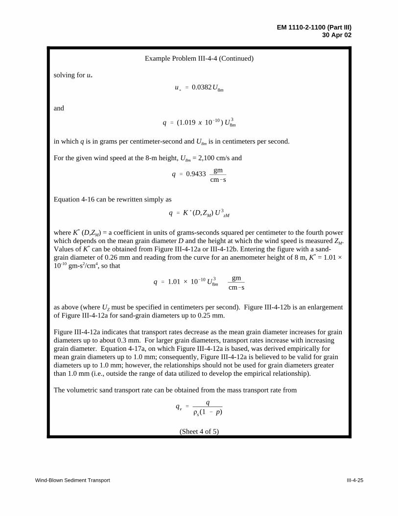
EM 1110-2-1100 (Part III)30 Apr 02
Wind-Blown Sediment Transport III-4-25
u(' 0.0382U8m
q ' (1.019 x 10&10 ) U 38m
q ' 0.9433 gmcm&s
q ' K ( (D,ZM) U 3zM
q ' 1.01 × 10&10 U 38m
gmcm&s
qv 'q
ρs (1 & p)
Example Problem III-4-4 (Continued)
solving for u*
and
in which q is in grams per centimeter-second and U8m is in centimeters per second.
For the given wind speed at the 8-m height, U8m = 2,100 cm/s and
Equation 4-16 can be rewritten simply as
where K* (D,ZM) = a coefficient in units of grams-seconds squared per centimeter to the fourth powerwhich depends on the mean grain diameter D and the height at which the wind speed is measured ZM. Values of K* can be obtained from Figure III-4-12a or III-4-12b. Entering the figure with a sand-grain diameter of 0.26 mm and reading from the curve for an anemometer height of 8 m, K* = 1.01 ×10⁻¹⁰ gm-s2/cm4, so that
as above (where UZ must be specified in centimeters per second). Figure III-4-12b is an enlargementof Figure III-4-12a for sand-grain diameters up to 0.25 mm.
Figure III-4-12a indicates that transport rates decrease as the mean grain diameter increases for graindiameters up to about 0.3 mm. For larger grain diameters, transport rates increase with increasinggrain diameter. Equation 4-17a, on which Figure III-4-12a is based, was derived empirically formean grain diameters up to 1.0 mm; consequently, Figure III-4-12a is believed to be valid for graindiameters up to 1.0 mm; however, the relationships should not be used for grain diameters greaterthan 1.0 mm (i.e., outside the range of data utilized to develop the empirical relationship).
The volumetric sand transport rate can be obtained from the mass transport rate from
(Sheet 4 of 5)

EM 1110-2-1100 (Part III)30 Apr 02
III-4-26 Wind-Blown Sediment Transport
qv '(0.9433)
(2.65) (1 & 0.4)or qv ' 0.5933 cm 3/cm&s
qv ' 5.933 × 10&5 m 3/m&s
qv ' Kv((D,ZM) U 3
zM
qv ' 6.3 × 10&15 U8m3
qv ' 6.3 × 10&15 (2,100)3 ' 5.83 × 10&5 m 3/m&s
U8mt ' 727.0 cm/s
q ' (1.019 × 10&10) U8m3 gm/cm&s
Example Problem III-4-4 (Concluded)
in which ρs = the mass density of the sand and p = the porosity (the fraction of the in situ sanddeposit which is pore space). Assuming a typical porosity of 0.4 for the in situ sand and using ρs =2.65 gm/cm3, the volume rate of dry sand transport per unit width is
Therefore
An equation for the volume sand transport rate can be written
in which Kv* = a coefficient in units of m2 - sec2/cm3 which depends on the mean sand-grain diameter
D and the height at which the wind speed is measured ZM. The coefficient Kv* can be obtained from
Figure III-4-13 which is based on the assumption that the sediment has a mass density of ρs =2.65 gm/cm2 and an in situ porosity of 0.4. Entering Figure III-4-13 with the grain diameter of0.26 mm and reading from the curve for an anemometer height of 8 m gives
in which qv = the volume transport rate in cubic meters per meter-second and U8m is in centimetersper second. Therefore
which is approximately the same result obtained earlier. Note that the wind speed is specified incentimeters per second and the resulting volume transport is in cubic meters per meter-second.
While the foregoing involves a lot of computation, repeated application of the equations to windspeed and direction data is much simplified, since the equations for the given site reduce to
the threshold wind velocity at the 8-m height, and
the mass transport rate per unit width where U8m is in centimeters per second. These equations willbe used in a subsequent example.
(Sheet 5 of 5)

EM 1110-2-1100 (Part III)30 Apr 02
Wind-Blown Sediment Transport III-4-27
Figure III-4-11a. Threshold (critical) wind speed as a function of median sand-grain diameter andthe anemometer height at which wind speed is measured (Continued)
1800
1600
1400 o"" ~'IJ
"" 0"' '<' 0<;0-
ov <v"' 1200 ~
~
u w (J) ~_,;;:-'1--0' ~
= ,d' u "'" ~ 1000 "'"<!-0 ~o~<v w w ~c""" Q_ (J)
0 z 800 5 0 _j
0 :r:: (f) w 600 [L :r:: f-
400
200
0 +-------4-------~--------+--------+-------+ 0 .2 .4 .6 .8
MEDIAN SAND GRAIN DIAMETER (MM)

EM 1110-2-1100 (Part III)30 Apr 02
III-4-28 Wind-Blown Sediment Transport
Figure III-4-11b. (Concluded)
800
700
u bi 600 ~
= u ~
0 w
it 500 [I)
0 z 5:
'3 400 0 :r:: [I) w [L :r:: f--
300
200
100
0
0
1 I
.05 . 1 . 1 5 .2 .25
MEDIAN SAND GRAIN DIAMETER (MM)

EM 1110-2-1100 (Part III)30 Apr 02
Wind-Blown Sediment Transport III-4-29
Figure III-4-12a. Mass transport rate coefficient K* as a function of median sand-grain diameter andthe anemometer height at which wind speed is measured (Continued)
1Q-8 +---------+-------~---------+---------r--------~
" = u ~ N
u w Ul
I
= Cl
f-z w u u_ u_ w 0 u w C;: cr fer 0 o_ Ul z <( cr f--
~ <( z 0 Ul z w
1 o-s
= 1 o- 10
0
10- 11 +----------f-----------r---------+---------+---------+ 0 .2 .4 .6 .8
MEDIAN SAND GRAIN DIAMETER (MM)

EM 1110-2-1100 (Part III)30 Apr 02
III-4-30 Wind-Blown Sediment Transport
Figure III-4-12b. (Concluded)
'" = u
" N
u w (f)
I
= Cl
f-z w u LL LL w 0 u w 10-9 C;;: rr fer 0 o_ (f)
z C2 HocHr c- -- ""2m _j <( z 0 (f)
z w = 0
1 o-11
0 .05 . 1 . 1 5 .2
MEDIAN SAND GRAIN DIAMETER (MM)
.25

EM 1110-2-1100 (Part III)30 Apr 02
Wind-Blown Sediment Transport III-4-31
Figure III-4-13. Volume transport rate coefficient K*V as a function of median sand-grain diameter
and the anemometer height at which wind speed is measured (assumes sediment density = 2.65gm/cm3 and porosity = 0.4)
10- 11 +--------r-------+--------r-------+--------r-------+
n
= u
" N
u w Ul
I
fz w u u_ u_ w 0 u fer
1 o-12 I
0 1 o-13 o_ Ul z <( cr f-
w = ::::l _j
0 > _j <( z 0 ~ 1 o-14
w = 0
--4m----
10-15+--------r-------+--------r-------+--------r-------+ 0 .05 .1 .15 .2 .25 .3
MEDIAN SAND GRAIN SIZE (MM)

EM 1110-2-1100 (Part III)30 Apr 02
III-4-32 Wind-Blown Sediment Transport
q ' (1.019 × 10&10) U8m3
EXAMPLE PROBLEM III-4-5
Find:
The total amount of sand transported by the wind during the given day and the total transported ineach of the 16 point compass directions.
Given:
Hourly wind speed and direction data given in Table III-4-3 for Westhampton Beach, Long Island,NY, were measured by an anemometer located 8 m above the ground. The median sand-grain diameterat Westhampton Beach is 0.26 mm.
Solution:
The solution is given in Table III-4-4. The preceding example problem shows that for a sand-graindiameter of 0.26 mm, the threshold wind speed at the 8-m height is 7.27 m/s. Winds less than 7.27 m/swill not transport sand. Columns 1, 2, and 3 in Table III-4-4 are the given data. (Note that winddirections are the direction from which the wind is blowing.) Column 4 is constructed from column 3and indicates the direction in which the sand will move rather than the direction from which the windis blowing. The given winds are essentially from the south and will transport sand northward. Column5 gives the effective winds. Winds less than the threshold value of 7.27 m/sec have been set to zero.Column 6 is computed from column 5 using the equation
in which U8m is the wind speed at the 8-m height in centimeters per second; this equation gives q ingrams per centimeter-seconds. Column 7 is obtained from column 6 by dividing by the density of thesand, 2.65 gm/cm3, and the packing factor, (1 - 0.4) = 0.6. The total volume transported during eachhour between observations (column 8) is 3,600 s/hr times the average transport rate during each hour.The total sand transport during the day is 0.5994 m3/m. Transport in each compass direction is givenat the bottom of the table.

EM 1110-2-1100 (Part III)30 Apr 02
Wind-Blown Sediment Transport III-4-33
Table III-4-3Hourly Wind Data, Westhampton Beach, Long Island, NY
Time (hr)Wind Speed
(m/sec)
WindDirection(Azimuth)
TransportDirection
(Compass)
(1) (2) (3) (4)*
Midnight 12.0 175 N
1 8.0 170 N
2 9.0 175 N
3 11.0 150 NNW
4 9.0 175 N
5 9.0 190 N
6 10.0 170 N
7 9.0 185 N
8 6.0 165 NNW
9 5.0 155 NNW
1 4.0 170 N
1 5.0 195 NNE
Noon 9.0 215 NE
1 14.0 200 NNE
2 12.0 215 NE
3 13.0 190 N
4 11.0 180 N
5 10.0 160 NNW
6 7.0 180 N
7 11.0 170 N
8 16.0 175 N
9 14.0 175 N
10 9.0 175 N
11 9.0 150 NNW
Midnight 7.0 145 NW
* Direction of transport (opposite of wind direction).

EM 1110-2-1100 (Part III)30 Apr 02
III-4-34 Wind-Blown Sediment Transport
Table III-4-4Hourly Transport Analysis Under Dry Conditions, Westhampton Beach, Long Island, NY
Time
(hr)(1)
Speed
(cm/sec)(2)
DirectionAzimuth
(3)
DirectionCompass
(4)
EffectiveWinds
(cm/sec)(5)
Rate
(g/cm-sec)(6)
Rate
(m3/m-sec)(7)
Volume
(m3/m) (8)
1 am 800 170 N 800 0.0522 3.281e-06 0.0258
2 900 175 N 900 0.0743 4.672e-06 0.0143
3 1100 150 NNW 1100 0.1356 8.530e-06 0.0238
4 900 175 N 900 0.0743 4.672e-06 0.0238
5 900 190 N 900 0.0743 4.672e-06 0.0168
6 1000 170 N 1000 0.1019 6.409e-06 0.0199
7 900 185 N 900 0.0743 4.672e-06 0.0199
8 600 165 NNW 0 0 0.000e+00 0
9 500 155 NNW 0 0 0.000e+00 0
10 400 170 N 0 0 0.000e+00 0
11 500 195 NNE 0 0 0.000e+00 0
Noon 900 215 NE 900 0.0743 4.672e-06 0.0084
1 pm 1400 200 NNE 1400 0.2796 1.759e-05 0.0401
2 1200 215 NE 1200 0.1761 1.107e-05 0.0516
3 1300 190 N 1300 0.2239 1.408e-05 0.0453
4 1100 180 N 1100 0.1356 8.530e-06 0.0407
5 1000 160 NNW 1000 0.1019 6.409e-06 0.0269
6 700 180 N 0 0 0.000e+00 0
7 1100 170 N 1100 0.1356 8.530e-06 0.0154
8 1600 175 N 1600 0.4174 2.625e-05 0.0626
9 1400 175 N 1400 0.2796 1.759e-05 0.0789
10 900 175 N 900 0.0743 4.672e-06 0.0401
11 900 150 NNW 900 0.0743 4.672e-06 0.0168
Midnight 700 145 NW 0 0 0.000e+00 0
TOTAL 0.5711
TOTAL NW 0
TOTAL NNW 0.0675
TOTAL N 0.4035
TOTAL NNE 0.0401
TOTAL NE 0.0600

EM 1110-2-1100 (Part III)30 Apr 02
Wind-Blown Sediment Transport III-4-35
u(tw ' u
(t % 18.75 cm/s
u(tw ' 27.75 % 18.75 ' 46.5 cm/s
u(tw ' 0.044U2mtw
U2mtw '46.5
0.044' 1057 cm/s
u('
κ (UZ2 & UZ1)ln (Z2 /Z1)
46.5 '0.4(U8mtw & 1057)
ln(8/2) Therefore U8mtw ' 1,218 cm/s
EXAMPLE PROBLEM III-4-6
Find:If the amount of precipitation on the given day exceeds the amount of evaporation, determine the
total amount of sand transported by wind and the amount of transport in each of the 16 compassdirections.
Given:The hourly wind speeds and directions in the preceding example problem (Table III-4-3) for
Westhampton Beach, Long Island.
Solution:Because the amount of precipitation exceeds the amount of evaporation, the sand can be assumed
to be wet and the threshold velocity will be greater than the threshold velocity for dry sand. Thethreshold velocity for wet sand is given by Equation 4-22b
in which u*tw and u*t are in centimeters per second. From the preceding example, u*t = 27.75 cm/s. Thus
The corresponding wind speed at the 2-m height is
or
For winds measured at the 8-m height, as before
and
The wind speed measured at the 8-m height must exceed 1,218 cm/s in order to transport sand. Windsless than 1,218 cm/s in the record are not considered in the computations. The wet sand thresholdvelocity can also be found from Figures III-4-14a or III-4-14b. Entering with a grain diameter of0.26 mm, read the curve for and anemometer height of 8 m to find the threshold velocity of U8mtw = 1,220cm/s. Figure III-4-14b is an enlargement of Figure III-4-14a. Table III-4-5 gives the results of thetransport analysis. Wet conditions reduce the total transport from 0.5994 m3/m to 0.2718 m3/m.
(Sheet 1 of 4)

EM 1110-2-1100 (Part III)30 Apr 02
III-4-36 Wind-Blown Sediment Transport
Figure III-4-14. Wet sand transport rate coefficient as a function of median sand graindiameter and the anemometer height at which wind speed is measured (Continued)
Example Problem III-4-6 (Continued)
(Sheet 2 of 4)

EM 1110-2-1100 (Part III)30 Apr 02
Wind-Blown Sediment Transport III-4-37
Figure III-4-14. (Concluded)
Example Problem III-4-6 (Continued)
(Sheet 3 of 4)

EM 1110-2-1100 (Part III)30 Apr 02
III-4-38 Wind-Blown Sediment Transport
Example Problem III-4-6 (Concluded)
Table III-4-5Hourly Transport Analysis Under Wet Conditions, Westhampton Beach, Long Island, NY.
Time
(hr)(1)
Speed
(cm/sec)(2)
DirectionAzimuth
(3)
DirectionCompass
(4)
EffectiveWinds
(cm/sec)(5)
Rate
(g/cm-sec)(6)
Rate
(m3/m-sec)(7)
Volume
(m3/m) (8)
1 am 800 170 N 0 0 0.000e+00 02 900 175 N 0 0 0.000e+00 03 1100 150 NNW 0 0 0.000e+00 04 900 175 N 0 0 0.000e+00 05 900 190 N 0 0 0.000e+00 06 1000 170 N 0 0 0.000e+00 07 900 185 N 0 0 0.000e+00 08 600 165 NNW 0 0 0.000e+00 09 500 155 NNW 0 0 0.000e+00 010 400 170 N 0 0 0.000e+00 011 500 195 NNE 0 0 0.000e+00 0
Noon 900 215 NE 0 0 0.000e+00 01 pm 1400 200 NNE 1400 0.2796 1.759e-05 0.0317
2 1200 215 NE 0 0 0.000e+00 03 1300 190 N 1300 0.2239 1.408e-05 0.02534 1100 180 N 0 0 0.000e+00 05 1000 160 NNW 0 0 0.000e+00 06 700 180 N 0 0 0.000e+00 07 1100 170 N 0 0 0.000e+00 08 1600 175 N 1600 0.4174 2.625e-05 0.04739 1400 175 N 1400 0.2796 1.759e-05 0.0789
10 900 175 N 0 0 0.000e+00 011 900 150 NNW 0 0 0.000e+00 0
Midnight 700 145 NW 0 0 0.000e+00 0
TOTAL 0.1832TOTAL NW 0
TOTALNNW
0
TOTALN
0.1515
TOTALNNE
0.0317
TOTALNE
0
(Sheet 4 of 4)

EM 1110-2-1100 (Part III)30 Apr 02
Wind-Blown Sediment Transport III-4-39
u(tw ' u
(t % 7.5W (III-4-21)
u(tw ' u
(t % 0.1875 (m/s) (III-4-22a)
u(tw ' u
(t % 18.75 (cm/s) (III-4-22b)
measurements were taken, and solve for Uz2t = the critical wind velocity at the Z2 height.) Only wind speedsin excess of the computed Uz2t will result in sand transport.
g. If wind speeds exceed the critical value and there was no precipitation on a given day, compute thepotential sand transport rate using Equation 4-16 or Equation 4-18.
h. If there was precipitation on a given day, the amount of precipitation should be compared with theamount of evaporation. If evaporation exceeds precipitation, compute the potential sand transport rate usingEquation 4-16 or 4-18. (If daily evaporation data are not available, daily evaporation can be estimated bydividing monthly evaporation by the number of days in the month.)
i. If precipitation exceeds evaporation, the critical shear velocity can be computed by
in which W = the fraction water content in the upper 5 mm of the sand (Hotta et al. 1985). Based onmeasurements in Holland made with a radioactive moisture probe, Svasek and Terwindt (1974) found thatW < 0.025 (2.5 percent). Consequently
or
may be used in the absence of detailed soil moisture data. For days when precipitation exceeds evaporation,u*tw is used as the critical shear velocity rather than u*t. The computations then proceed as above.
j. If precipitation is in the form of snow, there will be no sand transport until the snow cover has melted.In the computations, days with snow and days known to have snow cover are excluded from the record. Dataon snow cover are included in “Local Climatological Data” for all major National Weather Service (NWS)stations.
k. The results of a comprehensive study of potential sand transport by wind at Westhampton Beach byHsu (1994) are shown in the form of a transport rose in Figure III-4-15. The rose gives the direction fromwhich the sand is transported with the most being transported northward or northwestward. Wind data wereobtained from C_MAN Station ALSN6 for 1989. The results of the analysis are tabulated in Tables III-4-6through III-4-8. Table III-4-6 presents the results obtained by not considering snow cover or moistureconditions. The total potential transport for the year is 71.2 m3/m-yr. The table also shows that mosttransport at Westhampton Beach occurs during the winter months, with the most transport during Novemberand December. Table III-4-7 corrects for days of snow cover. The total transport is reduced to 64.6 m3/m-yr.When the data are also corrected for moisture conditions (Table III-4-8), the total transport is further reducedto 53.2 m3/m-yr, about 75 percent of the uncorrected value of 71.2 m3/m-yr.
III-4-5. Wind-Blown Sand Transport and Coastal Dunes
a. Dunes and dune processes.
(1) Sand dunes are important coastal features that are created, enlarged, and altered by wind-blown sand.In the absence of dunes, the beach landward of the active shoreface and berm is often characterized by a

EM 1110-2-1100 (Part III)30 Apr 02
III-4-40 Wind-Blown Sediment Transport
Figure III-4-15. Wind-blown sand transport rose at Westhampton Beach, Long Island, NY, for 1989(Hsu 1994)
w
WIND -BLOWN SAND TRANSPORT IN m3m-1 yr-1
AT WESTHAMPTON, LONG ISLAND,
N
NEW YORK, IN 1989 --+-~~ -1 yr - \-
:1 0' 7-G 0'
LEGEND: MAX. POTENTIAL TRANSPORT
EXCLUDE SNOW DAYS BUT INCLUDE BOTH WET
AND DRY TRANSPORTS
s
!-----+------1 E

EM 1110-2-1100 (Part III)30 Apr 02
Wind-Blown Sediment Transport III-4-41
Table III-4-6Monthly Sand Transport at Westhampton Beach, Long Island, NY (All Data Considered) (Hsu 1994)
Volume, Cubic Meters Per Meter
Direction Jan Feb Mar Apr May Jun Jul Aug Sep Oct Nov Dec Total
N 2.66 1.06 0.80 0.91 0.33 0.16 0.07 0.09 0.85 0.69 2.88 3.37 13.88
NE 0.14 1.45 1.12 0.38 0.12 0.03 0.15 0.14 0.10 0.24 0.34 0.86 5.07
E 0.92 0.63 3.94 0.13 1.83 0.33 0.23 0.60 1.63 2.41 0.04 0.33 13.01
SE 0.10 0.00 0.16 0.09 0.05 0.01 0.18 0.06 0.14 0.20 0.03 0.00 1.03
S 0.33 0.47 0.08 0.19 0.56 0.09 0.03 0.01 0.52 0.53 1.20 0.30 4.32
SW 0.47 0.95 1.68 2.09 1.54 0.58 0.28 0.12 1.53 0.58 1.67 0.33 11.82
W 0.33 0.30 0.20 0.10 0.24 0.02 0.16 0.08 0.18 0.42 1.85 0.34 4.23
NW 1.65 1.43 0.54 1.04 0.44 0.34 0.01 0.11 0.08 1.17 4.55 6.46 17.82
Total 6.62 6.29 8.53 4.94 5.11 1.55 1.10 1.22 5.03 6.24 12.56 11.99 71.18
Table III-4-7Monthly Sand Transport at Westhampton Beach, Long Island, NY (Snow Days Excluded) (Hsu 1994)
Volume, Cubic Meters Per Meter
Direction Jan Feb Mar Apr May Jun Jul Aug Sep Oct Nov Dec Total
N 2.66 0.76 0.78 0.91 0.33 0.16 0.07 0.09 0.85 0.69 2.80 3.12 13.24
NE 0.11 0.28 0.26 0.38 0.12 0.03 0.15 0.14 0.10 0.24 0.00 0.85 2.66
E 0.22 0.60 3.35 0.13 1.83 0.33 0.23 0.60 1.63 2.41 0.04 0.07 11.45
SE 0.10 0.00 0.16 0.09 0.05 0.01 0.18 0.06 0.14 0.20 0.03 0.00 1.03
S 0.33 0.47 0.08 0.19 0.56 0.09 0.03 0.01 0.52 0.53 1.20 0.30 4.32
SW 0.47 0.95 1.68 2.09 1.54 0.58 0.28 0.12 1.53 0.58 1.62 0.33 11.77
W 0.33 0.30 0.20 0.10 0.24 0.02 0.16 0.08 0.18 0.42 1.68 0.16 3.88
NW 1.65 1.18 0.54 1.04 0.44 0.34 0.01 0.11 0.08 1.17 4.27 5.40 16.23
Total 5.90 4.54 7.06 4.94 5.11 1.55 1.10 1.22 5.03 6.24 11.64 10.23 64.58
Table III-4-8Monthly Sand Transport at Westhampton Beach, Long Island, NY (Snow Days and Wet Days Excluded) (Hsu 1994)
Volume, Cubic Meters Per Meter
Direction Jan Feb Mar Apr May Jun Jul Aug Sep Oct Nov Dec Total
N 2.54 0.64 0.59 0.73 0.25 0.16 0.07 0.08 0.77 0.69 2.72 3.12 12.36
NE 0.11 0.27 0.19 0.19 0.00 0.03 0.05 0.08 0.08 0.00 0.00 0.85 1.85
E 0.22 0.49 2.89 0.00 1.00 0.02 0.04 0.49 1.00 2.14 0.00 0.07 8.37
SE 0.02 0.00 0.11 0.01 0.01 0.01 0.15 0.06 0.14 0.04 0.00 0.00 0.55
S 0.08 0.31 0.08 0.09 0.33 0.00 0.02 0.01 0.46 0.25 1.15 0.27 3.06
SW 0.44 0.70 1.30 1.86 1.44 0.23 0.28 0.10 1.19 0.32 0.83 0.24 8.93
W 0.23 0.28 0.20 0.09 0.22 0.01 0.06 0.08 0.18 0.30 1.24 0.13 3.03
NW 1.53 1.18 0.52 0.91 0.32 0.30 0.01 0.09 0.08 1.06 3.74 5.26 15.00
Total 5.17 3.87 5.89 3.88 3.56 0.76 0.67 1.00 3.90 4.81 9.69 9.95 53.15

EM 1110-2-1100 (Part III)30 Apr 02
III-4-42 Wind-Blown Sediment Transport
EXAMPLE PROBLEM III-4-7
Find:
Estimate the sand transport in each of the eight compass directions. (Note that the results of thisanalysis will only be approximate since no information on moisture conditions and/or snow cover isavailable. Also, the data are daily average wind speeds rather than hourly values.) Ideally, this typeof analysis would be performed with several years of hourly wind data; however, a rough estimatecan be obtained from wind rose data.
Given:
The wind rose for Atlantic City, NJ, in Figure III-4-16 and the median sand grain diameter of0.25 mm. The winds have been corrected to offshore conditions and the standard anemometer heightof 10 m.
Solution:
Data from the wind rose (Figure III-4-16) are tabulated in Table III-4-9. The transport rates atthe wind speed interval boundaries are computed in Table III-4-10. An upper bound of 35 mph wasselected to determine the average transport rate over the interval. This upper bound is somewhatarbitrary and was selected only 6 mph above the 29 mph lower bound since it is likely that on thosedays with average winds exceeding 29 mph, the speed will not exceed 29 mph by much. Column 3of Table III-4-10 gives the threshold wind speed at the 10-m height for a median sand-grain diameterof 0.25 mm. The transport coefficient in column 4 is from Figure III-4-12b. Column 5 is thetransport rate and column 6 is the average transport rate over the interval. (Note that it is importantto use average transport rates rather than average wind speeds since transport rate varies with thecube of the wind speed.) For example, the average transport rate over the interval between windspeeds of 29 mph and 35 mph is 0.2944 gm/cm-s. The amounts of sand transported are computed inTable III-4-11.
The threshold velocity of 7.25 m/s is greater than the 6.26 m/s corresponding to the 6.3 m/s (14 mph)interval boundary; therefore, the number of days that the wind speed was between 7.25 m/s and12.96 m/s (29 mph) was calculated assuming that wind speeds are uniformly distributed over theinterval. Adjusted days/year were computed as (12.96 - 7.25)/(12.96 - 6.26) = 0.852 times the totalnumber of days in the 6.3 m/s (14 mph) < U < 13.0 m/s (29 mph) interval. Column 5 is from TableIII-4-10. The mass transport (column 6) is column 5 x number of days x number of seconds/day. Column 7 is the volume transport equal to column 6 divided by (0.6) x 2.65 gm/cm3 and converted tocubic meters per meter. The total amount of sand transported in all directions is 146.1 m3/m.

EM 1110-2-1100 (Part III)30 Apr 02
Wind-Blown Sediment Transport III-4-43
Figure III-4-16. Wind Rose for Atlantic City, NJ (data from 1936 to 1952)
w
Oto14mph
- 14 to 29 mph
11111111111111 > 2 9 m p h

EM 1110-2-1100 (Part III)30 Apr 02
III-4-44 Wind-Blown Sediment Transport
Table III-4-9Wind Rose Data, Atlantic City, NJ (Wind Data, 1936 to 1952)
Direction Wind Speed Interval Days/Year
N 29 mph < U 3
N 14 mph < U < 29 mph 20
N 0 mph < U < 14 mph 20
NE 29 mph < U 5
NE 14 mph < U < 29 mph 19
NE 0 mph < U < 14 mph 11
E 29 mph < U 2
E 14 mph < U < 29 mph 15
E 0 mph < U < 14 mph 17
SE 29 mph < U 2
SE 14 mph < U < 29 mph 13
SE 0 mph < U < 14 mph 16
S 29 mph < U 3
S 14 mph < U < 29 mph 49
S 0 mph < U < 14 mph 25
SW 29 mph < U 1
SW 14 mph < U < 29 mph 23
SW 0 mph < U < 14 mph 12
W 29 mph < U 1
W 14 mph < U < 29 mph 42
W 0 mph < U < 14 mph 27
NW 29 mph < U 1
NW 14 mph < U < 29 mph 21
NW 0 mph < U < 14 mph 17
TOTAL 365
Table III-4-10Wind Rose Data Analysis, Atlantic City, NJ (Anemometer at Standard 10-m Height)
WindSpeed(mph)
WindSpeed(m/sec)
ThresholdWind Speed *
(m/sec)
TransportCoef. *
(gm-s2/cm4)
TransportRate
(gm/cm-sec)
Average RateOver Interval(gm/cm-sec)
(1) (2) (3) (4) (5) (6)
35 15.64 7.25 9.8000e-11 0.3753
0.2944
29 12.96 7.25 9.8000e-11 0.2135
0.1254
14 6.26 7.25 9.8000e-11 0.0373 **
0 ***
0 0 7.25 9.8000e-11 0
* Based on median grain size of 0.25 mm** Calculated for threshold wind speed of 7.25 m/s.*** Wind speed in interval does not exceed threshold wind speed.

EM 1110-2-1100 (Part III)30 Apr 02
Wind-Blown Sediment Transport III-4-45
Tabl
e III
-4-1
1W
ind
Blo
wn
Sand
Tra
nspo
rt A
naly
sis,
Win
d R
ose
Dat
a, A
tlant
ic C
ity, N
J (W
ind
Dat
a, 1
936
to 1
952)
Win
dD
irect
ion
Win
d Sp
eed
Inte
rval
Day
s/Ye
arA
djus
tmen
tD
ays/
Year
Tran
spor
tR
ate
(gm
/cm
-sec
)
Mas
sTr
ansp
ort
(gm
/cm
-yr)
Volu
me
Tran
spor
t(m
3 /m-y
r)
Dire
ctio
n in
whi
ch s
and
istr
ansp
orte
d(m
3 /m)
(1)
(2)
(3)
(4)
(5)
(6)
(7)
(8)
N 1
3 m
/s <
U
33
0.29
4476
,308
4.80
N6.
3 m
/s <
U <
13
m/s
2017
*0.
1254
184,
621
11.6
1To
tal S
= 1
6.41
N 0
m/s
< U
< 6
.3 m
/s20
00
00
NE
13
m/s
< U
5
50.
2944
127,
181
8.00
NE
6.3
m/s
< U
< 1
3 m
/s19
16*
0.12
5417
5,39
011
.03
Tota
l SW
= 1
9.03
NE
0 m
/s <
U <
6.3
m/s
110
00
0
E 1
3 m
/s <
U
22
0.29
4450
,872
3.20
E6.
3 m
/s <
U <
13
m/s
1513
*0.
1254
138,
466
8.71
Tota
l W =
11.
91
E 0
m/s
< U
< 6
.3 m
/s17
00
00
SE 1
3 m
/s <
U
22
0.29
4450
,872
3.20
SE6.
3 m
/s <
U <
13
m/s
1311
*0.
1254
120,
004
7.55
Tota
l NW
= 1
0.75
SE 0
m/s
< U
< 6
.3 m
/s16
00
00
S 1
3 m
/s <
U
33
0.29
4476
,308
4.80
S6.
3 m
/s <
U <
13
m/s
4942
*0.
1254
452,
321
28.4
5To
tal N
= 3
3.25
S 0
m/s
< U
< 6
.3 m
/s25
00
00
SW 1
3 m
/s <
U
11
0.29
4425
,436
1.60
SW6.
3 m
/s <
U <
13
m/s
2320
*0.
1254
212,
314
13.3
5To
tal N
E =
14.9
5
SW 0
m/s
< U
< 6
.3 m
/s12
00
00
W 1
3 m
/s <
U
11
0.29
4425
,436
1.60
W6.
3 m
/s <
U <
13
m/s
4236
*0.
1254
387,
704
24.3
8To
tal E
= 2
5.98
W 0
m/s
< U
< 6
.3 m
/s27
00
00
NW
13
m/s
< U
1
10.
2944
25,4
361.
60
NW
6.3
m/s
< U
< 1
3 m
/s21
18*
0.12
5419
3,85
212
.19
Tota
l SE
= 13
.79
NW
0 m
/s <
U <
6.3
m/s
170
00
0
Tota
l36
519
014
6.07
* Num
ber o
f day
s w
hen
win
d sp
eed
exce
eds
the
thre
shol
d w
ind
spee
d an
d so
me
trans
port
occu
rs.
Assu
mes
uni
form
dis
tribu
tion
of w
ind
spee
ds o
ver t
he 6
.3 m
/s <
U <
13
m/s
inte
rval
.

EM 1110-2-1100 (Part III)30 Apr 02
III-4-46 Wind-Blown Sediment Transport
“deflation plain” from which sand is removed and the profile lowered by wind. The presence of vegetationor other obstructions to the wind results in sand being trapped and leads to the creation of sand dunes.Foredunes are the first line of dunes landward of the shoreline. These dunes often result from the naturalaccumulation of wind-blown sand originating on the beach face; however, they may also be man-made.Whether natural or man-made, they are subject to continued growth, alteration, and movement due to naturalwind transport processes. When present and if sufficiently large, foredunes can provide protection fromcoastal flooding, shoreline erosion, and wave damage. Dunes can also shelter the area landward of them fromwind-blown sand by providing an area within which wind-blown sand accumulates. This can be an importantfunction of stabilized dunes, since wind-blown sand is often a nuisance that must be controlled.
(2) A line of dunes can provide protection from flooding due to high-water levels and wave overtopping.Sand stored in dunes is also available as a sacrificial contribution to the increased longshore and offshore sandtransport during storms. Dunes, by contributing their volume to the sand in transport, reduce the landwardmovement of the shoreline during storms. Dunes can also reduce wave damage in developed landward areasby limiting wave heights by causing waves to break as they propagate over the dunes. On undevelopedbarrier islands, dunes provide a source of sand for overwash processes. During storms with elevated waterlevels, waves overtopping the dunes carry sand into the bay or lagoon behind a barrier island. Over a periodof time, this natural process results in landward migration of the island.
(3) Dunes can be constructed artificially by: (a) beach nourishment, (b) grading existing sand availableon the dry beach, or (c) “beach scraping” - removing sand from below the high-water line during low tide andusing it to construct a protective dune. In areas where there is sufficient sand and the beach is wide, dunescan be encouraged to develop by natural accumulation by planting dune grass or other vegetation, or byinstalling sand fences to trap the landward-blowing sand. The rate at which dunes grow depends on the rateat which sand is transported to the dune from the fronting beach and on the effectiveness of the vegetation,fencing, and/or the dune itself in retaining sand. Because of the effect of the dune on the wind field (see Fig-ure III-4-8) and the absence of a mobile sand supply on the landward side of coastal dunes, there is littletransport from the dune to the beach, even during periods when winds blow seaward. Coastal dunes generallygrow by trapping and accumulating sand on their seaward side; thus, they grow toward the source of sand -the fronting beach. If more than one line of foredunes is to be developed by natural accumulation, thelandward line of dunes must be constructed before the line closest to the shoreline is constructed, otherwisethe line closest to the shoreline will trap sand and keep it from reaching the more landward line.
(4) When designing a dune system intended to accumulate sand by natural wind transport processes, thedunes should be set back from the shoreline so that there is sufficient dry beach to provide a source of sand.A distance of 60 m between the toe of the dune and the high-water line has been recommended (ShoreProtection Manual 1984). This expanse of sand is often not available on many beaches so that lesserdistances must be accepted. At the very least, the toe of the foredune should be landward of the normalseasonal fluctuation of the shoreline. Narrow beaches are less effective sand sources and dune growth willbe slower. Typical rates of sand accumulation in dunes are about 2.5 to 7.5 m3/m-yr; however, rates as highas 25 m3/m-yr have been measured (Woodhouse 1978). Savage (1963) measured accumulations of 4.5 to 6m3/m over a period of 7 to 8 months using a single row of sand fencing. Savage and Woodhouse (1968)measured accumulations of 39 m3/m over a 3-year period in a multiple-fence experiment. This is an averageof 13 m3/m-yr; however, accumulation rates must have been higher than this average rate during portions ofthe 3-year period.
(5) Dunes that are intended to provide protection against flooding and erosion must be stabilized toprevent their deflation and/or landward migration. Stabilization is also necessary to control the landwardmovement of wind-blown sand into developed areas. Stabilization can be achieved using vegetation or sandfencing. Guidelines for dune creation and stabilization using vegetation are given by U.S. Army Corps of

EM 1110-2-1100 (Part III)30 Apr 02
Wind-Blown Sediment Transport III-4-47
qz ' q cosα
qzE ' qE cos(50E)qzSE ' qSE cos(5E)qzS ' qS cos(40E)
qzSW ' qSW cos(85E)
Figure III-4-17. Net sand transport at an angle α with the winddirection
EXAMPLE PROBLEM III-4-8
Find:If the shoreline azimuth at Atlantic City is θ = 50 deg (angle between north and the shoreline),
estimate the rate at which sand might accumulate in a dune field behind the beach. (As in the precedingexample, this type of analysis ideally should be done with hourly wind data.)
Given:The transport computations from the preceding Example Problem III-4-7 based on the wind rose at
Atlantic City, NJ.
Solution:The transport rate in a given direction is the transport rate times the cosine of the angle between the
wind direction and the given direction. See Figure III-4-17. For Atlantic City, shoreline alignment andcompass directions are shown in Figure III-4-18. For example, an easterly wind will transport sandperpendicular to the shoreline qzE = qE cos 50E where qzE is the transport perpendicular to the shorelineinto the dunes. For a southeasterly wind, the transport perpendicular to the shoreline is qzSE = qSEcos 5 deg. In general,
where α = angle between wind direction and offshore, directed normal to the shoreline.For the example
(Sheet 1 of 4)

EM 1110-2-1100 (Part III)30 Apr 02
III-4-48 Wind-Blown Sediment Transport
Figure III-4-18. Shoreline orientation with respect to compassdirections at Atlantic City, NJ
qz ' q cosα cos2β, 180E < β < 360E
cos(α) ' cos(β & 90E) ' & sin(β)
Example Problem III-4-8 (Continued)
Winds blowing generally from the dunes or backbeach towards the shoreline are not as efficient intransporting sand as are winds blowing generally onshore. This is because of sheltering provided by thedune itself and stabilization by vegetation on the dune, and because there is often only a limited supplyof sand landward of the dunes. This latter condition prevails at Atlantic City, where much of the arealandward of the beach is paved or developed. Figure III-4-8 also shows that in the lee of a dune, windsnear ground level may be in the direction opposite of the wind direction at a higher elevation. Windsblowing seaward from the dunes are not very efficient in transporting sand from the dunes back onto thebeach. Sand transport efficiency, proportional to the square of the cosine of the angle between the winddirection and a vector perpendicular to the shoreline, is assumed. See Figure III-4-19 for the efficiencyfactor as a function of β, the angle between the shoreline and wind direction. Figure III-4-20 gives thedefinition of β.
Sand transport rates in the offshore direction, perpendicular to the general orientation of the dune toe,are given by
where β is the angle the wind makes with the shoreline and α is the angle the wind makes with a vectorperpendicular to the shoreline. Therefore, α = β - 90E and
(Sheet 2 of 4)

EM 1110-2-1100 (Part III)30 Apr 02
Wind-Blown Sediment Transport III-4-49
qz ' & q sinβ cos2β, 180E < β < 360E
Figure III-4-19. Sand transport efficiency for winds blowingfrom dunes toward beach as a function of the angle betweenwind direction and shoreline
Figure III-4-20. Definition of angle ß, between wind and shoreline
Example Problem III-4-8 (Continued)Therefore,
The sin β term in the equation corrects the transport from the wind direction to a direction perpendicularto the shore, while the cos2 β term is the efficiency term introduced to consider the sheltering effects ofthe dune.
(Sheet 3 of 4)

EM 1110-2-1100 (Part III)30 Apr 02
III-4-50 Wind-Blown Sediment Transport
Example Problem III-4-8 (Concluded)
Results of the analysis are given in Table III-4-12. Columns 1 and 2 are obtained from Table III-4-11.Column 3 is the angle β between the given wind directions and the shoreline azimuth of θ = 50E atAtlantic City. Column 4 is sin(β) and column 5 is the offshore wind transport efficiency, cos2(β). Theefficiency is assumed equal to 1.0 for onshore winds. Column 6, the rate of dune growth due to windsfrom the given direction, is the product of columns 2, 4, and 5. The estimated total potential dune growthrate is 27.2 m3/m-yr. This estimate represents a potential growth rate which depends on the sand supply.The analysis does not consider the effects of snow cover and moisture to reduce transport. Woodhouse(1978) reports on a 30-year average dune accumulation rate of 13.7 m3/m-yr on the Clatsop Plains,Oregon, and suggests that higher accumulation rates probably prevailed in the early years.
Table III-4-12Estimated Annual Dune Growth at Atlantic City, NJ
WindDirection
AnnualTransport
(m3/m)
WindAngle (β)(degrees)
COS(α)or
SIN(ß)EfficiencyCOS²(ß)
DuneGrowth
(m3/m/yr)
(1) (2) (3) (4) (5) (6)
N 15.79 310 -0.7660 0.4132 -5.00
NE 18.44 355 -0.0872 0.9924 -1.60
E 11.44 40 0.6428 1.00001 7.35
SE 10.34 85 0.9962 1.00001 10.30
S 31.73 130 0.7660 1.00001 24.31
SW 14.24 175 0.0872 1.00001 1.24
W 24.68 220 -0.6428 0.5868 -9.31
NW 13.14 265 -0.9962 0.0076 -0.10
TOTAL 27.20 m3/m/yr
1 Transport efficiency = 1.0 for angles between 0 and 180 deg.
(Sheet 4 of 4)

EM 1110-2-1100 (Part III)30 Apr 02
Wind-Blown Sediment Transport III-4-51
Engineers (1978) and Woodhouse (1978). The best type of stabilizing vegetation varies with geographicalarea, location on the dune, exposure of the site, whether the water body is salt or fresh water, etc. Typicalplants used for dune stabilization include European beach grass (Ammophila arenaria) and, less frequently,American dunegrass (Elymus mollis) along the Pacific Northwest and California coasts; American beach grass(Ammophila breviligulita) along the mid- and upper-Atlantic and Great Lakes coasts; sea oats (Uniolapaniculata) along the South Atlantic and gulf coasts, and panic grasses (Panicum amarum or P. amarulum)along the Atlantic and gulf coasts.
(6) Guidelines for dune creation and stabilization with fencing are given in the Shore Protection Manual(1984) and Woodhouse (1978). Typical sand fencing is either wooden-slat fencing of the type used to controlsnow along highways or geosynthetic fabric fencing. A wooden-slat fence is typically 1.2 m high with 3.8-cm-wide slats wired together to provide about 50 percent porosity. Stabilization by fencing requires periodicinspection of the installation, replacement of damaged or vandalized fencing, and installation of new fencingto continue the stabilization process as the dune grows. The size and shape of a dune can be controlled bystategically installing subsequent lines of fencing to encourage the dune to grow higher or wider. Most fenceinstallations fill within 1 year of construction. Dune growth is most often limited by the available sand supplyrather than by the capacity of the fence installation. Dunes created by fencing must also subsequently beplanted to stabilize them for when the fencing eventually deteriorates.
(7) Stabilization by vegetation has the advantage that it is capable of growing up through theaccumulating dune and of repairing itself if damaged, provided the damage is not too extensive. Afterplanting and for a year or two thereafter, vegetation requires fertilization to establish healthy plants. Trafficthrough vegetated dunes must also be controlled to prevent damage to plants by excluding any pedestriansand vehicles or by providing dune walk-over structures. Dune areas with barren areas in an otherwise healthyvegetated dune, will be subject to “blowouts,” local areas of deflation. Blowouts reduce a dune's capabilityto protect an area from flooding.
(8) An example of estimating the rate of dune growth follows. Example III-4-8 assumes that all of thesand transported to the dune is trapped by vegetation and/or sand fencing and that the fronting beach issufficiently wide to supply sand at the potential transport rate for a given wind speed, i.e., dune growth is notlimited by sand supply. Subsequent examples consider the effects of armoring and a limited sand supply.
b. Factors affecting dune growth rates.
(1) The dune growth rates presented in the preceding section and Example III-4-8 are “potential” rates,since they consider only the accumulation of sand in the dunes and not any of the processes that remove sandfrom the dunes. Furthermore, the trapping process is assumed to be nearly perfect, i.e., little sand is removedfrom the dunes when wind direction reverses and blows offshore and no sand is blown landward of the dunes.In some developed coastal communities, sand is often removed from the area landward of the dunes; hence,the rate of dune growth often underestimates wind-blown sand transport rates or, vice versa, calculatedtransport rates overestimate the rate of dune growth. Some typical measured dune growth rates are given inTable III-4-13.
(2) On relatively narrow beaches backed by dunes, the dunes are occasionally eroded by waves duringstorms having elevated water levels. The storms often leave a nearly vertical scarp with the height of thescarp and the amount of erosion depending on the severity of the storm; i.e., the height of the waves and stormsurge. Less frequently, during unusual storms, the dune may be completely destroyed. Dunes erode duringstorms only to be rebuilt during the period between storms with sand transported by winds having an onshorecomponent. The net rate of dune growth, therefore, is only a fraction of what would be predicted if only ratesof accumulation are considered and sand losses are ignored. Dune growth rates can be estimated

EM 1110-2-1100 (Part III)30 Apr 02
III-4-52 Wind-Blown Sediment Transport
Table III-4-13Measured Dune Growth Rates (Field experiments conducted by Coastal Engineering Research Center in 1960sand 1970s)
Site Padre Island, TX Padre Island, TX Ocracoke Island, NC
Type Wood fencing(3 fences, 3 lifts)
Wood fencing(4 fences, 3 lifts)
American Beachgrass
Beach 60 - 90 m 60 - 90 m 180 - 210 m
GrowthRates
∆t(mos)
∆V(m3/m)
Rate(m3/m-yr)
∆t(mos)
∆V(m3/m)
Rate(m3/m-yr)
∆t(mos)
∆V(m3/m)
Rate(m3/m-yr)
12 8.5 8.53 12 6.0 6.02 24 12.8 6.40
12 6.8 6.77 12 10.3 10.28 27 9.8 4.35
12 10.8 10.79 12 6.5 6.52 29 16.6 6.85
Avg Rate 8.70 7.61 5.86
Site Core Banks, NC Padre Island, TX Core Banks, NC
Type American Beachgrassand fence
Sea oats Sea oats
Beach 120 - 150 m 60 - 90 m 90 m
GrowthRates
∆t(mos)
∆V(m3/m)
Rate(m3/m-yr)
∆t(mos)
∆V(m3/m)
Rate(m3/m-yr)
∆t(mos)
∆V(m3/m)
Rate(m3/m-yr)
32 11.7 4.42 36 29.6 9.87 22 5.0 2.74
22 11.0 4.98 60 42.6 8.53 14 2.8 2.37
26 10.8 4.98 19 6.3 3.96
Avg Rate 5.14 9.20 3.02
Site Clatsop Spit, OR
Type European beachgrass
Beach 180 m
GrowthRates
∆t(mos)
∆V(m3/m)
Rate(m3/m-yr)
360 384 12.79
Avg Rate 12.79
by constructing a sediment budget for the dune that balances rates of accumulation against rates of erosion.However, estimating the occurrence and volume of dune erosion is difficult. Estimating how much sand isactually trapped by the dune is also difficult.
(3) The rate at which sand is supplied to a dune depends also on the availability of a sand source upwindof the dunes. A wide beach usually provides an adequate source. However, if the beach is narrow, there maynot be a sufficient upwind supply in the sense that the over-sand fetch is insufficient for the transport rate toreach an equilibrium (Nordstrom and Jackson 1992; Gillette et al. 1996). Consequently, calculated transportrates overestimate actual transport rates.

EM 1110-2-1100 (Part III)30 Apr 02
Wind-Blown Sediment Transport III-4-53
Figure III-4-21. Schematic views of sorted sand deposits: (a)well-sorted (poorly graded); (b) poorly sorted (well-graded); (c)poorly sorted after fines have been removed by wind erosion
(4) The size gradation of the beach sand also has an influence on transport rates. Sand transport analysesbased on a single sand-grain diameter fail to recognize that beach sands are comprised of a gradation of sizeseach of which has a different threshold wind speed that initiates motion. Grains finer than the median sizeare more easily transported and may be moved by lower wind speeds while coarser grains are left behind.Basing transport rates on only the median grain size fails to recognize that finer grains on the surface can betransported even when wind speeds are relatively low. Ideally, each grain size should be consideredseparately. In addition, as fines are removed from the beach sand surface, the remaining larger size fractionarmors the surface, making it difficult to transport additional sand. Figure III-4-21(a) shows a relativelyuniform distribution of sand grains where almost all grains have about the same threshold speed. Figure III-4-21(b) shows a well-graded sand prior to wind erosion, while Figure III-4-21(c) shows the same well-gradedsand after the fines have been removed leaving behind the coarse fraction on the surface. Higher wind speedsare required to continue the transport process after the fine surficial materials are removed. Alternatively,processes that break up the beach surface to expose additional fine sediments to wind will reestablish thetransport of fines. Such processes include pedestrian and vehicular traffic and beach raking.
(5) The formation of a salt crust on the beach surface by the evaporation of seawater also increasesthreshold wind speeds and reduces transport (Nickling and Egglestone 1981). Sand below the high tide lineis most affected by this process; however, occasional saturation of the beach above the usual high tide levelby storm tides will expand the affected beach area inland. Additionally, salt spray carried inland by wind canfurther expand the affected area. Processes that break up the crust to restore usual threshold wind speedsinclude pedestrian and vehicular traffic.
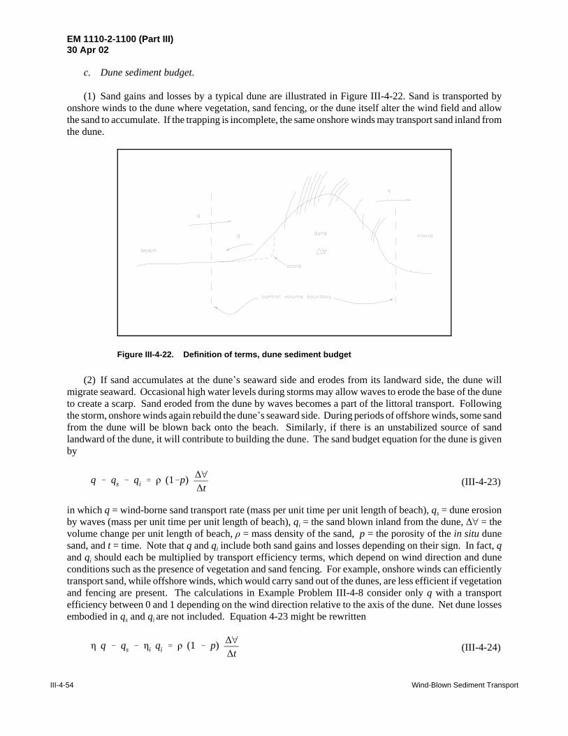
EM 1110-2-1100 (Part III)30 Apr 02
III-4-54 Wind-Blown Sediment Transport
Figure III-4-22. Definition of terms, dune sediment budget
q & qs & qi ' ρ (1&p) ∆œ∆t (III-4-23)
η q & qs & ηi qi ' ρ (1 & p) ∆œ∆t (III-4-24)
c. Dune sediment budget.
(1) Sand gains and losses by a typical dune are illustrated in Figure III-4-22. Sand is transported byonshore winds to the dune where vegetation, sand fencing, or the dune itself alter the wind field and allowthe sand to accumulate. If the trapping is incomplete, the same onshore winds may transport sand inland fromthe dune.
(2) If sand accumulates at the dune*s seaward side and erodes from its landward side, the dune willmigrate seaward. Occasional high water levels during storms may allow waves to erode the base of the duneto create a scarp. Sand eroded from the dune by waves becomes a part of the littoral transport. Followingthe storm, onshore winds again rebuild the dune*s seaward side. During periods of offshore winds, some sandfrom the dune will be blown back onto the beach. Similarly, if there is an unstabilized source of sandlandward of the dune, it will contribute to building the dune. The sand budget equation for the dune is givenby
in which q = wind-borne sand transport rate (mass per unit time per unit length of beach), qs = dune erosionby waves (mass per unit time per unit length of beach), qi = the sand blown inland from the dune, ∆œ = thevolume change per unit length of beach, ρ = mass density of the sand, p = the porosity of the in situ dunesand, and t = time. Note that q and qi include both sand gains and losses depending on their sign. In fact, qand qi should each be multiplied by transport efficiency terms, which depend on wind direction and duneconditions such as the presence of vegetation and sand fencing. For example, onshore winds can efficientlytransport sand, while offshore winds, which would carry sand out of the dunes, are less efficient if vegetationand fencing are present. The calculations in Example Problem III-4-8 consider only q with a transportefficiency between 0 and 1 depending on the wind direction relative to the axis of the dune. Net dune lossesembodied in qs and qi are not included. Equation 4-23 might be rewritten

EM 1110-2-1100 (Part III)30 Apr 02
Wind-Blown Sediment Transport III-4-55
Ra ' Tf Rt (III-4-25)
µφ 'φ16 % φ84
2(III-4-26)
σφ 'φ16 & φ84
2(III-4-27)
φ ' & log2 dmm
or equivalently by
φ ' &3.3219 log10 dmm
(III-4-28)
in which η = the transport efficiency for winds at the seaward side of the dune and ηi = the transport efficiencyfor winds at the landward side of the dune. For the calculations in Example Problem III-4-8, η was assumedto be a function of wind direction (η = 1 for winds with an onshore component and 0 < η < 1 for winds withan offshore component), and ηi was assumed zero (no inland sand losses and no inland sand source). Notethat η was assumed to vary as cos2β with 180 deg < β < 360 deg, where β = the angle between the wind andthe dune axis (the dunes are usually parallel with the shoreline) so that β = 270 deg represents wind blowingfrom the back of the dune.
d. Procedure to estimate dune “trapping factor.”
(1) Unfortunately, the preceding discussion assumes knowledge of quantities that are most typicallyunknown and a simple approach must be taken. A “dune trapping factor” can be computed to correctpredicted “potential” dune growth rates in order to obtain better estimates of actual rates. The trapping factorTf is based on the difference between the sand grain size distribution on the dune and the size distribution onthe beach in front of the dune. If Rt = a theoretical growth rate based on calculations of sand transport andRa = the actual growth rate, the relationship is given by
(2) The value of Tf can be found using the procedure suggested by Krumbein and James (1965) tocompare the characteristics of potential beach nourishment sand with native beach sand characteristics.While the Krumbein and James (1965) procedure has been superseded by better methods to estimate beachnourishment overfill ratios, in principle it presents a way to estimate what volume of sand with a givengradation is needed to produce a unit volume of sand having a different gradation. The procedure is basedon the assumption that the gradations of the sand on the beach and the sand in the dunes are both log-normallydistributed and can be described by their phi-mean µφ and phi-standard deviation σφ. These parameters canbe estimated using the relationships
and
in which φ16 = the phi diameter of the 16th percentile (16 percent of the grains are finer) and φ84 = the phidiameter of the 84th percentile. The phi diameter is given by
in which φ = the diameter in phi units and dmm = the grain diameter in millimeters. The phi-mean and phi-standard deviation are calculated for sand taken from the dune, FφD and σφD, and for sand from the beach infront of the dune, FφB and σφB , and the following parameters are calculated

EM 1110-2-1100 (Part III)30 Apr 02
III-4-56 Wind-Blown Sediment Transport
σφ D
σφ B(III-4-29)
µφ D & µφ B
σφ B(III-4-30)
Figure III-4-23. Dune sand trapping factor Tf
and
and used with Figure III-4-23 to determine how much beach sand is needed to produce a unit volume of dunesand. Figure III-4-23 is derived from the equation

EM 1110-2-1100 (Part III)30 Apr 02
Wind-Blown Sediment Transport III-4-57
φ ' &log2 dmm
φ ' & 3.3219 log10 dmm
φ16 ' & 3.3219 log10 (0.159) ' 2.65
φ84 ' 0.59
φ16 ' 2.53 and φ84 ' 1.31
µφB '2.65 % 0.59
2' 1.62
EXAMPLE PROBLEM III-4-9
Find:Determine the dune trapping factor and estimate the rate of dune growth for the sands from the beach
and dune in Atlantic City with the size characteristics given below.
Given:The dune growth rate from Example Problem III-4-8 based on the transport rates of Example
Problem III-4-7 and the following data from a sand size analysis of the beach and dune sands at AtlanticCity.
Beach sand: d16 = 0.159 mm d84 = 0.664 mm
Dune sand: d16 = 0.173 mm d84 = 0.403 mm
Solution:To use the relationships for Fφ and σn, the phi diameter must be calculated for each of the above
percentiles using Equation 4-28.
For the beach sand
or equivalently
and, therefore
Similarly
For the dune sand
From Equation III-4-26 and III-4-27
(Continued)

EM 1110-2-1100 (Part III)30 Apr 02
III-4-58 Wind-Blown Sediment Transport
σφB '2.65 & 0.59
2' 1.03
µφD ' 1.92 and σφD ' 0.61
Tf '0.611.03
exp (1.92 & 1.62)2
2(0.612 & 1.032)– 0.55
Ra ' 0.55 Rt
Ra ' 0.55 (27.2) – 15.0 m3
m&yr
Example Problem III-4-9 (Concluded)
and
Similarly, for the dune sand
Substituting these values into Equation 4-31 gives
The trapping factor Tf can also be found from Figure III-4-23.
Consequently, the transport rate found in example problem III-4-8 should be multiplied by 0.55. Thetransport rate is therefore
or

EM 1110-2-1100 (Part III)30 Apr 02
Wind-Blown Sediment Transport III-4-59
Tf 'σφ D
σφ B
exp(µφ D & µφ B )2
2 (σ2φ D & σ2
φ B )(III-4-31)
which is based on a comparison of the log-normal distributions of dune and beach sands. The procedure isvalid only if the dune sand is finer than the beach sand and more narrowly graded (better sorted). This isgenerally the case since the dune sand is almost always derived from the sand on the beach in front of thedune.
(3) Some example values of the various parameters for typical beach and dune sands along withcalculated dune trapping factors are given in Table III-4-14.
Table III-4-14Typical Beach and Dune Sand Phi Diameters and Dune Trapping Factors Calculated from Beach and Dune SandSamples at Various U. S. Beaches
Locationφ16
(dune)φ84
(dune)φ16
(beach)φ84
(beach) FφB FφD σφB σφD Tf
North StreetOcean City, NJ
2.48 1.88 2.61 1.72 2.17 2.18 0.45 0.30 0.67
9th StreetOcean City, NJ
2.59 0.79 2.49 0.19 1.34 1.69 1.15 0.90 0.69
29th StreetOcean City, NJ
2.64 1.98 2.69 1.41 2.05 2.31 0.64 0.33 0.46
36th StreetOcean City, NJ
2.53 1.31 2.65 0.59 1.62 1.92 1.03 0.61 0.55
Cape May, NJLocation 1
1.86 0.60 2.06 0.20 1.13 1.23 0.93 0.63 0.67
Cape May, NJLocation 2
1.62 0.58 1.71 0.39 1.05 1.10 0.66 0.52 0.78
CERC FRFDuck, NC
0.76 1.08 1.00 0.77 0.68
Clearwater Beach, FL 2.87 2.09 2.66 1.41 2.04 2.48 0.63 0.39 0.41
e. Continuity equation for wind transport of beach sand.
(1) The continuity equation for the beach sand transported by an onshore wind is developed inFigure III-4-24.
(2) At the upwind end of the fetch, the ocean and/or saturated sand precludes any wind transport. Furthershoreward, the sand is dry and transportable by the prevailing wind; however, the amount in transport hasnot reached its potential rate predicted by the equations. In this region the wind is deflating the beach. Theamount of sand leaving the ∆x-long control volume exceeds the amount entering and the difference iscomprised of sand eroded from the beach. Downwind along the fetch, the sand transport rate has reachedequilibrium and the amount of sand entering the control volume equals the amount leaving. Here the beachis not deflating; rather the amount of sand eroded is balanced by the amount deposited. Further along thefetch, near the base of the dune, the amount of sand entering the control volume is less than the amountremoved by the wind, and sand accumulates to build the dune. The change in transport rate is often due toa decrease in local wind speed induced by vegetation, sand fencing, or by the dune itself. Writing a sedimentbalance for the ∆x control volume yields the equation

EM 1110-2-1100 (Part III)30 Apr 02
III-4-60 Wind-Blown Sediment Transport
Figure III-4-24. Sand conservation equations for a beach showing deflation area,equilibrium area, and deposition area
q % qe & q %MqMx
∆x ' 0 (III-4-32)
MqMx
'qe
∆x(III-4-33)
qe 'MyM t
∆x ρ (1 & p) ε (III-4-34)
in which q equals the wind-blown transport into the control volume (mass per unit time per unit lengthperpendicular to the direction of transport), qe equals the amount contributed to the control volume by erosionfrom the beach (mass per unit time per unit length), and ∆x equals the width of the control volume in thedirection of transport. The first two terms are the sand influx to the control volume while the term in bracketsis the efflux. Simplifying Equation 4-32 gives
(3) The contribution from the beach qe can be expressed as a deflation rate times the beach surface area
in which y equals the height of the beach surface above some datum, ρ equals the mass density of the sand,p equals the porosity of the in-situ beach sand, and ε equals a dimensionless “erodibility factor” related to thebeach sand that is potentially transportable. ε is related to the sand size gradation as well as to any conditionsthat increase the threshold wind speed such as soil moisture content, salt crust formation, etc. Equation III-4-33 becomes

EM 1110-2-1100 (Part III)30 Apr 02
Wind-Blown Sediment Transport III-4-61
MqMx
'MyM t
ρ 1 & p ε (III-4-35)
(4) The upwind boundary condition, q = 0 at x = 0, is applied where the sand is first transportable, i.e.,at the shoreline or the point where the sand is no longer wet. Since different size fractions are transportedat different rates by a given wind speed, Equation 4-35 must be applied to each range of sizes present on thebeach. Unfortunately, the relationship between the size gradation parameters and the amount of surficial,transportable sand is not known. Therefore, it is not possible to establish limit depths of erosion for a givenwind speed blowing over sand with a given size distribution.
(5) The amount of sand available for transport at a given wind speed depends on the gradation as wellas the mean or median grain size. For a fine, poorly graded sand, once transport is initiated, there is a nearlycontinuous supply of sizes that can be transported. For a well-graded sand subjected to winds capable oftransporting the finer fractions, fine sediments are eventually removed from the surface leaving behind thecoarse fraction. See Figure III-4-21. In order to continue the transport process, higher wind speeds mustoccur or fine sediments must be exposed at the surface again.
f. Limited source due to gradation armoring. Beach sands generally are not uniform in size but havea gradation that is often log-normally distributed. The finer fraction at the beach surface is more easilytransported than the coarser fraction. Finer sand in the gradation also has the potential to be transported ata greater rate by lower wind speeds while larger sand is transported at a slower rate, if at all. However, asfiner sands are depleted from the surface layer of the beach, the remaining larger particles shelter theunderlying fines and armor the beach. Then, at the upwind end of the fetch, transport of fine sand ceases and,unless the wind speed increases to remove and transport the coarser fraction, transport will cease. Furtherdownwind, the fines leaving the control volume balance the fines entering so that transport continues.Consequently, there is a moving, upwind boundary between that portion of beach where the fines have beenremoved and transport has ceased, and where transport of fines continues. Each size fraction has its ownboundary. As fines are removed and the coarser fraction remains behind to armor the surface, the no-transport boundary moves downwind. Note that for sand with a uniform size gradation, this armoring processdoes not occur while for a well-graded sand it does. Other armoring processes may occur for uniformlygraded sands. Figure III-4-24 shows the location of the upwind boundary separating the armored area fromthe area where transport processes continue.

EM 1110-2-1100 (Part III)30 Apr 02
III-4-62 Wind-Blown Sediment Transport
Figure III-4-25. Beach and dune and size gradations for Atlantic City, NJ
EXAMPLE PROBLEM III-4-10
Find:The wind transport rate for each fraction of the sand at Atlantic City having the distribution given
in Figure III-4-25. Determine the total transport by summing the transport of all fractions using thebeach sand size distribution as a weight function.
Given:The wind rose data from Atlantic City in Table III-4-9 and the beach and dune sand size distributions
in Figure III-4-25.
Solution: The first step is to divide the size distribution for the beach sand into discrete increments and to
determine the threshold wind speed for the upper limit of each size interval. See Table III-4-15. Thevolumetric transport coefficient is obtained from Figure III-4-13 entering with the appropriate sand graindiameter and elevation at which the wind speeds are measured (in this example assumed to be 10 m).The wind speeds in both miles per hour (mph) and in centimeters per second at the wind rose intervalboundaries are given in Table III-4-16.
(Sheet 1 of 6)
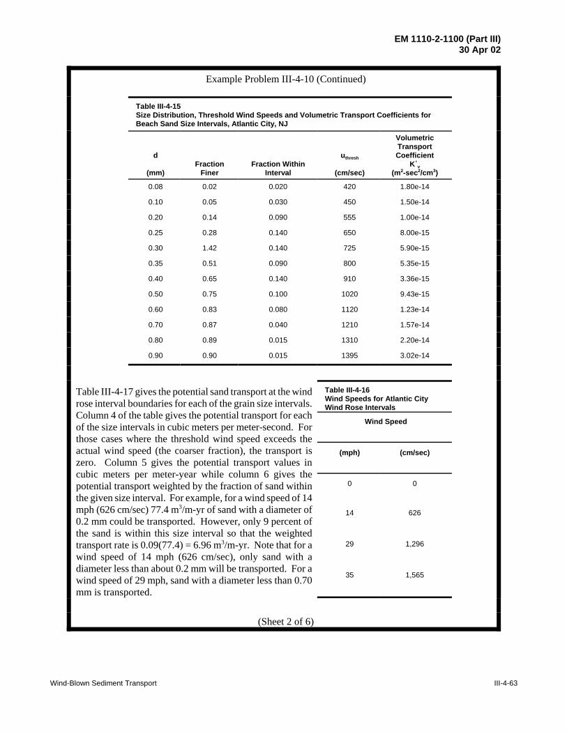
EM 1110-2-1100 (Part III)30 Apr 02
Wind-Blown Sediment Transport III-4-63
Example Problem III-4-10 (Continued)
Table III-4-15Size Distribution, Threshold Wind Speeds and Volumetric Transport Coefficients forBeach Sand Size Intervals, Atlantic City, NJ
d
(mm)Fraction
FinerFraction Within
Interval
uthresh
(cm/sec)
VolumetricTransportCoefficient
K*v(m2-sec2/cm3)
0.08 0.02 0.020 420 1.80e-14
0.10 0.05 0.030 450 1.50e-14
0.20 0.14 0.090 555 1.00e-14
0.25 0.28 0.140 650 8.00e-15
0.30 1.42 0.140 725 5.90e-15
0.35 0.51 0.090 800 5.35e-15
0.40 0.65 0.140 910 3.36e-15
0.50 0.75 0.100 1020 9.43e-15
0.60 0.83 0.080 1120 1.23e-14
0.70 0.87 0.040 1210 1.57e-14
0.80 0.89 0.015 1310 2.20e-14
0.90 0.90 0.015 1395 3.02e-14
Table III-4-17 gives the potential sand transport at the windrose interval boundaries for each of the grain size intervals.Column 4 of the table gives the potential transport for eachof the size intervals in cubic meters per meter-second. Forthose cases where the threshold wind speed exceeds theactual wind speed (the coarser fraction), the transport iszero. Column 5 gives the potential transport values incubic meters per meter-year while column 6 gives thepotential transport weighted by the fraction of sand withinthe given size interval. For example, for a wind speed of 14mph (626 cm/sec) 77.4 m3/m-yr of sand with a diameter of0.2 mm could be transported. However, only 9 percent ofthe sand is within this size interval so that the weightedtransport rate is 0.09(77.4) = 6.96 m3/m-yr. Note that for awind speed of 14 mph (626 cm/sec), only sand with adiameter less than about 0.2 mm will be transported. For awind speed of 29 mph, sand with a diameter less than 0.70mm is transported.
Table III-4-16Wind Speeds for Atlantic CityWind Rose Intervals
Wind Speed
(mph) (cm/sec)
0 0
14 626
29 1,296
35 1,565
(Sheet 2 of 6)

EM 1110-2-1100 (Part III)30 Apr 02
III-4-64 Wind-Blown Sediment Transport
Example Problem III-4-10 (Continued)Table III-4-17Transport Rates for Size Intervals at Atlantic City Wind Rose Speed Intervals
d
(mm)Fraction Within
Interval
Wind Speed
(cm/sec)
Potential Transport
(m3/m-sec)
Potential Transport
(m3/m-yr)
Transport Weightedby Sand Fraction
Within Interval(m3/m-yr)
0.08 0.020 626 4.413e-6 139.3 2.79
0.10 0.030 626 3.677e-6 116.0 3.48
0.20 0.090 626 2.451e-6 77.4 6.96
0.25 0.140 626 01 01 01
0.30 0.140 626 0 0 0
0.35 0.090 626 0 0 0
0.40 0.140 626 0 0 0
0.50 0.100 626 0 0 0
0.60 0.080 626 0 0 0
0.70 0.040 626 0 0 0
0.80 0.015 626 0 0 0
0.90 0.015 626 0 0 0
0.08 0.020 1296 3.922e-5 1237.7 24.75
0.10 0.030 1296 3.268e-5 1031.4 30.94
0.20 0.090 1296 2.179e-5 687.6 61.88
0.25 0.140 1296 1.743e-5 550.1 77.01
0.30 0.140 1296 1.286e-5 405.7 56.80
0.35 0.090 1296 1.166e-5 367.9 33.11
0.40 0.140 1296 7.321e-6 231.0 32.34
0.50 0.100 1296 2.055e-5 648.4 64.84
0.60 0.080 1296 2.680e-5 845.7 67.66
0.70 0.040 1296 3.421e-5 1079.5 43.18
0.80 0.015 1296 01 01 01
0.90 0.015 1296 0 0 0
0.08 0.020 1565 6.895e-5 2175.8 43.52
0.10 0.030 1565 5.746e-5 1813.2 54.40
0.20 0.090 1565 3.830e-5 1208.8 108.79
0.25 0.140 1565 3.064e-5 967.0 135.38
0.30 0.140 1565 2.260e-5 713.2 99.85
0.35 0.090 1565 2.049e-5 646.7 58.20
0.40 0.140 1565 1.287e-5 406.2 56.86
0.50 0.100 1565 3.612e-5 1139.9 113.99
0.60 0.080 1565 4.711e-5 1486.8 118.94
0.70 0.040 1565 6.014e-5 1897.8 75.91
0.80 0.015 1565 8.427e-5 2659.3 39.89
0.90 0.015 1565 1.157e-4 3650.5 54.761 Threshold wind speed exceeds actual wind speed and there is no transport of coarser sands.
(Sheet 3 of 6)

EM 1110-2-1100 (Part III)30 Apr 02
Wind-Blown Sediment Transport III-4-65
Example Problem III-4-10 (Continued)
Table III-4-18 is constructed from Table III-4-17 and the wind rose data. Table III-4-18 is only for windsfrom the north. The values in columns 2, 3, and 4 are the average transport values over the wind speedinterval; hence, for example, the first value in column 3 is the average transport over the wind speedinterval 14 mph < U < 29 mph, or (2.79 + 24.75)/2 = 13.77 m3/m-yr. Similarly, the first value in column 4is the average over the interval 29 mph < U < 35 mph, or (24.75 + 43.52)/2 = 34.14 m3/m-sec. The valuesin column 5 are the weighted sums of the values across each row with the number of days that the windwas within the given speed interval used as the weight factor. Hence, the value in the first row is givenby (1.395)(20/365) + (13.77)(20/365) + (34.14)(0/365) = 0.831 m3/m-yr. Consequently, the total amountof sand transported northward is 14.218 m3/m-yr. Table III-4-18 is for winds from the north only. Similaranalyses must be done for the remaining seven compass directions. The results of the analyses for all eightcompass directions are summarized in Table III-4-19 where, for example, column 2 is derived fromcolumn 5 of Table III-4-18. (Calculations for the remaining compass directions are omitted for brevity.)
Table III-4-18Wind Transport of Size Intervals for Winds from North Weighted by Fraction of Year Wind was withinGiven Speed and Direction Interval
(Similar tables must be constructed for the other seven compass directions)
Wind From North
d(mm)
Avg. Transport OverInterval0<U<14
No. Days = 20
Avg. Transport OverInterval
14<U<29No. Days = 20
Avg. TransportOver Interval
29<U<35No. Days = 0
Sum ofTransports
Weighted byNo. of Days
(m3/m-yr)
0.08 1.395 13.77 34.14 0.831
0.10 1.740 17.21 42.67 1.038
0.20 3.480 34.42 85.33 2.077
0.25 0 38.5 106.20 2.110
0.30 0 28.4 78.33 1.556
0.35 0 16.55 45.66 0.907
0.40 0 16.17 44.60 0.886
0.50 0 32.42 89.42 1.776
0.60 0 33.83 93.30 1.854
0.70 0 21.59 59.55 1.183
0.80 0 0 19.95 0
0.90 0 0 27.38 0
TOTAL N = 14.218
(Sheet 4 of 6)

EM 1110-2-1100 (Part III)30 Apr 02
III-4-66 Wind-Blown Sediment Transport
Example Problem III-4-10 (Continued)
Table III-4-19Summary of Transports for Eight Compass Directions
d(mm) Transport (m2/yr)
N NE E SE S SW W NW
0.08 0.831 1.226 0.818 0.739 2.225 1.007 1.781 0.951
0.10 1.038 1.533 1.022 0.923 2.780 1.259 2.226 1.188
0.20 2.077 3.066 2.044 1.846 5.560 2.517 4.452 2.376
0.25 2.110 3.456 2.164 1.953 6.041 2.717 4.721 2.506
0.30 1.556 2.551 1.596 1.441 4.456 2.004 3.483 1.849
0.35 0.907 1.487 0.930 0.840 2.597 1.168 2.029 1.077
0.40 0.886 1.453 0.909 0.820 2.537 1.141 1.983 1.053
0.50 1.776 2.912 1.822 1.645 5.087 2.288 3.975 2.110
0.60 1.854 3.039 1.902 1.716 5.308 2.387 4.148 2.202
0.70 1.183 1.940 1.214 1.095 3.388 1.524 2.647 1.405
0.80 0 0.273 0.109 0.109 0.164 0.055 0.055 0.055
0.90 0 0.375 0.150 0.150 0.225 0.075 0.075 0.075
TOTAL 14.218 23.314 14.680 13.277 40.307 18.142 31.576 16.847
Dune growth depends on the wind direction relative to the dune axis and the assumptions made regardingthe ability of the dune to trap and hold sand. The procedures presented in Example Problem III-4-8 areapplied to each individual grain size interval and the values summed to estimate the amount of sandtrapped by the dune. Transport in each direction is multiplied by sinβ, the angle between the dune axisand the direction from which the wind is blowing, and cos2β, the dune trapping efficiency. These valuesare given at the bottom of Table III-4-20. The values in Table III-4-20 are the net contribution to dunegrowth by winds from the indicated directions. For example, winds from the north remove sand from thedunes since values in column 2 are negative (the wind is blowing from the dune toward the beach). Forthis site, most dune growth is due to southerly winds and, to a lesser extent, to southeasterly winds.
(Sheet 5 of 6)

EM 1110-2-1100 (Part III)30 Apr 02
Wind-Blown Sediment Transport III-4-67
Example Problem III-4-10 (Concluded)
For the example, the total dune growth rate is 38.63 m3/m-yr. This represents a high rate ofgrowth and most certainly overestimates dune growth at Atlantic City since the example assumesan unlimited supply of sand in all size intervals available for transport. As in ExampleProblem III-4-9, the calculated dune growth rate can be adjusted by using the trapping efficiencybased on a comparison of the beach sand with the dune sand. From the preceding example, Tf =0.55; hence, the estimated dune growth rate is Ra = 0.55(38.63) = 21.4 m3/m-yr. An alternativeprocedure to adjust dune growth rates based on comparing the dune sand distribution with thebeach sand distribution is given in Example Problem III-4-11, which follows.
Table III-4-20Computation of Dune Growth Rate
d(mm)
Dune Growth (m2/yr)
N NE E SE S SW W NW Total
0.08 -0.263 -0.106 0.526 0.736 1.704 0.088 -0.672 -0.007 2.110
0.10 -0.329 -0.133 0.657 0.919 2.130 0.110 -0.840 -0.009 2.639
0.20 -0.657 -0.265 1.314 1.839 4.260 0.219 -1.679 -0.018 5.277
0.25 -0.668 -0.299 1.391 1.946 4.628 0.237 -1.781 -0.019 5.734
0.30 -0.493 -0.221 1.026 1.435 3.144 0.175 -1.314 -0.014 4.230
0.35 -0.287 -0.129 0.598 0.836 1.989 0.102 -0.766 -0.008 2.465
0.40 -0.280 -0.126 0.584 0.817 1.944 0.100 -0.748 -0.008 2.408
0.50 -0.562 -0.252 1.171 1.638 3.897 0.199 -1.500 -0.016 2.828
0.60 -0.587 -0.263 1.222 1.710 4.066 0.208 -1.565 -0.011 5.038
0.70 -0.374 -0.168 0.780 1.091 2.595 0.133 -0.999 -0.010 3.215
0.80 0 -0.024 0.070 0.109 0.126 0.005 -0.021 -0.000 0.288
0.90 0 -0.032 0.096 0.150 0.172 0.007 -0.028 -0.001 0.396
TOTAL -4.500 -2.017 9.436 13.226 30.925 1.581 -11.911 -0.127
sinβ -0.7660 -0.0872 0.6428 0.9962 0.7660 0.0872 -0.6428 -0.9962
cos2β 0.4132 0.9924 1.0000 1.0000 1.0000 1.0000 0.5868 0.0076
TOTAL DUNE GROWTH RATE = 38.631 m3/m-yr
(Sheet 6 of 6)

EM 1110-2-1100 (Part III)30 Apr 02
III-4-68 Wind-Blown Sediment Transport
EXAMPLE PROBLEM III-4-11
Find:
The trapping efficiency for natural dune building in Atlantic City and the dune grain size distributioncalculated from the results of Example Problem III-4-10 given the measured and calculated grain-sizedistributions for the dune sand at Atlantic City.
Given:The dune growth rates based on the individual grain size intervals as calculated in Example
Problem III-4-10 and the actual dune sand size distributions given in Figure III-4-25.
Solution: The calculated amounts of sand trapped in the dune from each size interval are given in
Table III-4-21. The values in column 2 of Table III-4-21 are found by summing across the rows inTable III-4-20. Thus, 2.111 m3/m-yr of sand with a diameter less than 0.08 mm is trapped by the dunes.Similarly, 2.639 m3/m-yr of sand with a diameter between 0.08 mm and 0.10 mm is trapped. Thecalculated size distribution of the dune sand is determined by normalizing the values in column 2 bydividing each value in column 2 by the sum of column 2. The resulting values are given in column 3,which represents the fraction of the sand in the dune within the given size interval. For example, 0.0547or 5.47 percent of the dune sand is finer than d = 0.08 mm and 6.83 percent is between d = 0.10 mm andd = 0.08 mm, etc. Column 4 of Table III-4-21 gives the cumulative distribution.
Table III-4-21Calculated Dune Sand Size Distribution
d(mm)
Amount Trapped in Dune(m3/m-yr)
Normalized AmountTrapped in Dune
Cumulative SizeDistribution
in Dune
0.08 2.111 0.0547 0.05470.10 2.639 0.0683 0.12300.20 5.277 0.1366 0.25960.25 5.732 0.1484 0.40800.30 4.230 0.1095 0.51750.35 2.465 0.0638 0.58130.40 2.408 0.0623 0.64360.50 4.828 0.1250 0.76860.60 5.038 0.1304 0.89900.70 3.215 0.0832 0.98230.80 0.288 0.0075 0.98980.90 0.396 0.0102 1.0000
TOTAL 38.631 1.0000
(Sheet 1 of 4)

EM 1110-2-1100 (Part III)30 Apr 02
Wind-Blown Sediment Transport III-4-69
Figure III-4-26. Actual and calculated dune sand size gradation at Atlantic City, NJ
Example Problem III-4-11 (Continued)
Figure III-4-26 shows the calculated sand size distribution in the dune along with the actual dune sizedistribution. The actual distribution differs from the calculated distribution because not all of the sandpresent on the beach is available for transport due to processes like gradation armoring, crust formation,etc. Some fines might be confined between larger grains and once the surficial fines are removed, theremaining fines are not available for transport. Also, the coarser fraction can only be transported by theless frequent high wind speeds.
The transport rates calculated for each size interval are potential transport rates. Comparison of thecalculated size distribution with the actual distribution allows a correction factor to be calculated for eachsize fraction. Columns 2 and 3 of Table III-4-22 present the calculated and actual size distributions,respectively. Column 4 is a calculated correction factor equal to the actual interval fraction divided bythe calculated interval fraction. For example, the correction factor 0.1818 in the first row equals0.0100/0.0547, the ratio of column 3 over column 2. Thus column 4 gives the numbers by whichcalculated values must be multiplied in order to obtain actual values. The amount of sand available fortransport in each size interval is limited, so, in order to calculate the amount actually transported in eachsize interval, the correction factor values in column 4 must be normalized by dividing through by thelargest value. (Column 4 would suggest that 300 percent of the amount of sand between 0.35 mm and0.40 mm is needed to produce the observed distribution. Clearly, no more than 100 percent can beavailable.) The values in column 5 result. These values can be considered to be transport correctionfactors for each size interval. They are the values by which the transport rate in each size interval mustbe multiplied in order to produce the measured dune size distribution.
(Sheet 2 of 4)

EM 1110-2-1100 (Part III)30 Apr 02
III-4-70 Wind-Blown Sediment Transport
Example Problem III-4-11 (Continued)
Table III-4-22Comparison of Calculated Dune Sand Size Distribution and Actual Dune Sand SizeDistribution
d(mm)
Calculated DuneSand Size
Distribution
Actual DuneSand Size
DistributionCorrection =
Actual/CalculatedNormalizedCorrection
0.08 0.0547 0.0100 0.1818 0.0604
0.10 0.0683 0.0470 0.6912 0.2297
0.20 0.1366 0.1355 0.9891 0.3286
0.25 0.1484 0.0908 0.6135 0.2039
0.30 0.1095 0.2250 2.0455 0.6797
0.35 0.0638 0.1334 2.1175 0.7036
0.40 0.0623 0.1896 3.0095 1.0000
0.50 0.1250 0.0832 0.6656 0.2212
0.60 0.1304 0.0397 0.3054 0.1015
0.70 0.0832 0.0125 0.1506 0.0500
0.80 0.0075 0.0125 1.6026 0.5325
0.90 0.0102 0.0100 0.9804 0.3258
TOTAL 1.0000 1.0000
Table III-4-23 gives the corrected transport rates for each size interval. Column 2 is the calculated amountin each size interval trapped in the dune. (See column 2, Table III-4-21.) Column 3 is the normalizedcorrection factor (see column 5, Table III-4-22) and column 4 is the corrected dune growth rate for sandwithin the given size fraction. The sum of the values in column 4 gives the corrected dune growth rate.For the given example, the corrected dune growth rate is 12.7 m3/m-yr. This procedure is similar to theprocedure used to derive the trapping factor Tf but by matching the calculated and actual dune sizedistributions and without assuming that the distributions are log-normal. The value of Tf can be calculatedfor this example by taking the ratio of the value of the total from column 4 in Table III-4-23 to the totalin column 2. This ratio is Tf = 12.68/38.63 = 0.33, which can be computed with the value of Tf = 0.57calculated in Example Problem III-4-9.
Figure III-4-27 compares the actual dune size distribution with the calculated distribution after thecorrection has been applied.
(Sheet 3 of 4)

EM 1110-2-1100 (Part III)30 Apr 02
Wind-Blown Sediment Transport III-4-71
Figure III-4-27. Comparison of actual dune sand size gradation with corrected,calculated gradation
Example Problem III-4-11 (Concluded)
Table III-4-23Corrected Transport Rates for Size Intervals and Corrected Dune Growth Rate
d(mm)
CalculatedTransport Rates
(m3/m-yr)
NormalizedCorrection
Factor
CorrectedTransport Rates
(m3/m-yr)
0.08 2.111 0.0604 0.12750.10 2.639 0.2297 0.60620.20 5.277 0.3286 1.73400.25 5.732 0.2039 1.16880.30 4.230 0.6797 2.87510.35 2.465 0.7036 1.73440.40 2.408 1.0000 2.40800.50 4.828 0.2212 1.06800.60 5.038 0.1015 0.51140.70 3.215 0.0500 0.16080.80 0.288 0.5325 0.15340.90 0.396 0.3258 0.1290
TOTAL = 38.627 12.6766
(Sheet 4 of 4)
EM 1110-2-1100 (Part III)30 Apr 02
III-4-72 Wind-Blown Sediment Transport
III-4-6. References
EM 1110-2-5003Planting Guidelines for Dune Creation and Stabilization
Bagnold 1936Bagnold, R. A. 1936. “The Movement of Desert Sand,” Proceedings Royal Society of London, Series A, Vol157, pp 94-620.
Bagnold 1941Bagnold, R. A. 1941. The Physics of Blown Sand and Desert Dunes, Morrow, New York, (republished in1954 by Methuen, London).
Belly 1962Belly, P. Y. 1962. “Sand Movement by Wind,” Technical Memorandum, TM-1, Coastal and HydraulicsLaboratory, U.S. Army Engineer Waterways Experiment Station, Vicksburg, MS.
Chapman 1990Chapman, D. M. 1990. “Aeolian Sand Transport - An Optimized Model,” Earth Surface Processes andLandforms, Vol 15, pp 751-760.
Gillette, Herbert, Stockton, and Owen 1996Gillette, D. A., Herbert, G., Stockton, P. H., and Owen, P. R. 1996. “ Causes of the Fetch Effect in WindErosion,” Earth Surface Processes and Landforms, Vol 21, pp 641-659.
Holzworth 1972Holzworth 1972. “Mixing Heights, Wind Speeds, and Potential for Urban Air Pollution Throughout theContiguous United States,” Office of Air Programs, Publication No. AP-101, Environmental ProtectionAgency, Research Triangle Park, North Carolina.
Horikawa 1988Horikawa, K. (Editor). 1988. Nearshore Dynamics and Coastal Processes, University of Tokyo Press,Tokyo, Japan.
Horikawa and Shen 1960Horikawa, K., and Shen, H. W. 1960. “Sand Movement by Wind Action - on the Characteristics of SandTraps,” Technical Memorandum 119, Coastal and Hydraulics Laboratory, U.S. Army Engineer WaterwaysExperiment Station, Vicksburg, MS.
Hotta, Kubota, Katori, and Horikawa 1985Hotta, S., Kubota, S., Katori, S., and Horikawa, K. 1985. “Sand Transport by Wind on a Wet Sand Surface,”Proceedings, 19th International Conference on Coastal Engineering, American Society of Civil Engineers,pp 1265-1281.
Hsu 1973Hsu, S. A. 1973. “Computing Eolian Sand Transport from Shear Velocity Measurements,” Journal ofGeology, Vol 81, pp 739-743.

EM 1110-2-1100 (Part III)30 Apr 02
Wind-Blown Sediment Transport III-4-73
Hsu 1977Hsu, S. A. 1977. “Boundary Layer Meteorological Research in the Coastal Zone,” Geoscience and Man,H. J. Walker, ed., School of Geoscience, Louisiana State University, Baton Rouge, LA, Vol 18, pp 99-111.
Hsu 1981Hsu, S. A. 1981. “Models for Estimating Offshore Winds from Onshore Meteorological Measurements,”Boundary Layer Meteorology, Vol 20, pp 341-351.
Hsu 1986Hsu, S. A. 1986. “Correction of Land-Based Wind Data for Offshore Applications: A Further Evaluation,”Journal of Physical Oceanography, Vol 16, pp 390-394.
Hsu 1988Hsu, S. A. 1988. Coastal Meteorology, Academic Press, San Diego, CA.
Hsu 1994Hsu, S. A. 1994. Personal communication, Coastal Studies Institute, Louisiana State University,Baton Rouge, LA.
Hsu and Blanchard 1991Hsu, S. A., and Blanchard, B. W. 1991. “Shear Velocity and Eolian Sand Transport on a Barrier Island,”Proceedings, Coastal Sediments ‘91, American Society of Civil Engineers, New York, Vol 1, pp 220-234.
Kadib 1964Kadib, A. 1964. “Calculation Procedure for Sand Transport on Natural Beaches,” Miscellaneous Paper 2-64,Coastal and Hydraulics Laboratory, U.S. Army Engineer Waterways Experiment Station, Vicksburg, MS.
Kadib 1966Kadib, A. 1966. “Mechanics of Sand Movement on Coastal Dunes,” Journal of the Waterways and HarborsDivision, American Society of Civil Engineers, WW2, pp 27-44.
Kawamura 1951Kawamura, R. 1951. “Study on Sand Movement by Wind,” Report, Institute of Science and Technology,University of Tokyo. (translation, University of California, Berkeley, Hydraulic Engineering LaboratoryResearch Report, HEL-2-9, Berkeley, CA, 1964, pp 1-64).
Krumbein and James 1965Krumbein, W. C., and James, W. R. 1965. “A Lognormal Size Distribution Model for Estimating Stabilityof Beach Fill Material,” TM-16, Coastal and Hydraulics Laboratory, U.S. Army Engineer WaterwaysExperiment Station, Vicksburg, MS.
Liu, Schwab, and Bennett 1984Liu, P. C., Schwab, D. J., and Bennett, J. R. 1984. “Comparison of a Two Dimensional Wave PredictionModel with Synoptic Measurements in Lake Michigan,” Journal of Physical Oceanography, Vol 14,pp 1514-1518.

EM 1110-2-1100 (Part III)30 Apr 02
III-4-74 Wind-Blown Sediment Transport
Nickling and Egglestone 1981Nickling, W. G., and Egglestone, M. 1981. “The Effects of Soluble Salts on the Threshold Shear Velocityof Fine Sand,” Sedimentology, Vol 28, pp 505-510.
Nordstrom and Jackson 1992Nordstrom, K. F., and Jackson, N. L. 1992. “Effect of Source Width and Tidal Elevation Changes onAeolian Transport on an Estuarine Beach,” Sedimentology, Vol 39, pp 769-778.
O'Brien and Rindlaub 1936O'Brien, M. P., and Rindlaub, B. D. 1936. “The Transport of Sand by Wind,” Civil Engineering, Vol 6,pp 325-327.
Powell 1982Powell, M. D. 1982. “The Transition of the Hurricane Frederic Boundary-Layer Wind Field from the OpenGulf of Mexico to Landfall,” Monthly Weather Review, Vol 110, pp 1912-1932.
Raudkivi 1976Raudkivi, A. J. 1976. Loose Boundary Hydraulics, 2nd ed., Pergamon Press, New York.
Resio and Vincent 1977Resio, D.T., and Vincent, C. L. 1977. “Estimation of Winds Over the Great Lakes,” Journal of theWaterway, Port, Coastal and Ocean Engineering Division, American Society of Civil Engineers, Vol 103,No. WW2.
Sarre 1988Sarre, R. D. 1988. “Evaluation of Eolian Transport Equations Using Intertidal Zone Measurements: SauntonSands, England,” Sedimentology, Vol 35, pp 671-679.
Savage 1963Savage, R. P. 1963. “Experimental Study of Dune Building with Sand Fences,” Proceedings, InternationalConference on Coastal Engineering, 1963, pp 380-396.
Savage and Woodhouse 1968Savage, R. P., and Woodhouse, W. W., Jr. 1968. “Creation and Stabilization of Coastal Barrier Dunes,”Proceedings, 11th International Conference on Coastal Engineering, Vol 1, 1968, pp 671-700.
SethuRaman and Raynor 1980SethuRaman, S., and Raynor, G. S. 1980. “Comparison of Mean Wind Speeds and Turbulence at a CoastalSite and Offshore Location,” Journal of Applied Meteorology, Vol 19, pp 15-21.
Shore Protection Manual 1984Shore Protection Manual. 1984. 4th ed., 2 Vol, U.S. Army Engineer Waterways Experiment Station, U.S.Government Printing Office, Washington, DC.
Svasek and Terwindt 1974Svasek, J.N., and Terwindt, J. H. J. 1974. “Measurements of Sand Transport by Wind on a Natural Beach,”Sedimentology, Vol 21, pp 311-322.

EM 1110-2-1100 (Part III)30 Apr 02
Wind-Blown Sediment Transport III-4-75
Wieringa 1980Wieringa, J. 1980. “Representativeness of Wind Observation at Airports,” Bulletin, AmericanMeteorological Society, Vol 61, pp 962-971
Williams 1964Williams, G. 1964. “Some Aspects of the Aeolian Saltation Load,” Sedimentology, Vol 3, pp 257-287.
Woodhouse 1978Woodhouse, Jr. 1978. “Dune Building and Stabilization with Vegetation,” Special Report No. 3, Coastaland Hydraulics Laboratory, U.S. Army Engineer Waterways Experiment Station, Vicksburg, MS.
Zingg 1953Zingg, A. W. 1953. “Wind Tunnel Studies of the Movement of Sedimentary Material,” Proceedings, 5thHydraulic Conference, State University of Iowa, Studies in Engineering, Bulletin, Vol 34, pp 111-135.

EM 1110-2-1100 (Part III)30 Apr 02
III-4-76 Wind-Blown Sediment Transport
III-4-7. Definition of Symbols
∆œ Volume change per unit length of beach [length3/length]
g Erodibility factor related to beach sand that is potentially transportable[dimensionless]
η Transport efficiency for winds at the seaward side of a dune
ηi Transport efficiency for winds at the landward side of a dune
κ von Karman’s constant (= 0.4)
µn Mean of a sediment sample [phi units]
µnD or B Mean of a sediment sample taken from the dune or beach [phi units]
νa Kinematic viscosity of air [length2/time]
ρ Mass density of sediment grains [force-time2/length4]
ρa Mass density of air [force-time2/length4]
σn Standard deviation of a sediment sample [phi units]
σnD or B Standard deviation of a sediment sample taken from the dune or beach [phi units]
τ Boundary shear stress [force/length2]
n Sediment grain diameter in phi units (n = -log2 dmm, where dmm is the grain diameterin millimeters)
nx Sediment grain diameter of the x-percentile of a sample (x-percent of the grains arefiner) [phi units]
A Empirical constant (Equation III-4-10) [dimensionless]
At Dimensionless constant ( = 0.118) used in calculating the critical shear stress, u*t ,for sand transport by wind (Equation III-4-20)
B Empirical constant (Equation III-4-10) [dimensionless]
BBagnold Bagnold coefficient [dimensionless]
CD,land Drag coefficients over land [dimensionless]
CD,sea Drag coefficient over sea [dimensionless]
Cz Wind drag coefficient at height Z (Equation III-4-4) [dimensionless]
d Standard grain size ( = 0.25mm)
D Median sediment grain diameter [length - generally millimeters]
D Mean sediment grain diameter [length - generally millimeters]
dmm Sediment grain diameter in millimeters

EM 1110-2-1100 (Part III)30 Apr 02
Wind-Blown Sediment Transport III-4-77
dx Sediment grain diameter of the x-percentile of a sample (x-percent of the grains arefiner) [length]
e Base of natural logarithms
g Gravitational acceleration (32.17 ft/sec2, 9.807m/sec2) [length/time2]
G Dry weight sand transport rate [force/length/time]
Hland Height of the planetary boundary layer over the land [length]
Hsea Height of the planetary boundary layer over the sea [length]
K Empirical dimensional eolian sand transport coefficient (Equation III-4-17)[force/length/time]
KN Eolian sand transport coefficient (Equation III-4-19) [dimensionless]
n Empirically determined exponent (ranging from 1/11 to 1/17) (Equation III-4-15)[dimensionless]
p Porosity of the in situ dune sand [percent]
q Wind-borne sand transport rate [mass/time/length]
qi Sand blown inland from the dune [mass/time/length]
qs Dune erosion by waves [mass/time/length]
qv Volumetric sand transport rate [length3/length/time]
Ra Actual dune growth rate [length3/length-time]
Rt Theoretical dune growth rate [length3/length-time]
RT Temperature correction factor applied to wind speed at the 10-m height (Figure III-4-7) [dimensionless]
t Time
Ta Air temperature [degrees Celsius]
Tf Dune trapping factor [dimensionless]
Ts Sea temperature [degrees Celsius]
u* Wind shear or friction velocity [length/time]
u*t Critical or threshold velocity for sand transport by wind (Equation III-4-20)[length/time]
u*tw Critical or threshold velocity for wet sand transport by wind (Equation III-4-20)[length/time]
Uland Wind speed over land [length/time]
Usea Wind speed over sea [length/time]

EM 1110-2-1100 (Part III)30 Apr 02
III-4-78 Wind-Blown Sediment Transport
Ux Average wind speed at x-elevation [length/time]
Uz Average wind velocity as a function of height above ground level [length]
UZM Wind speed at the anemometer height [length/time]
U!10m Wind speed at the 10-meter height corrected for the air-sea temperature difference[length/time]
W Fraction of water content in the upper 5mm of the sand [percent]
Z Height at which wind speed is measured [length]
Z0 Height of a roughness element characterizing the surface over which the wind isblowing [length]
ZM Anemometer height [length]
ZR Reference height [length]
ZZingg Zingg Coefficient [dimensionless]

EM 1110-2-1100 (Part III)30 Apr 02
Wind-Blown Sediment Transport III-4-79
III-4-8. Acknowledgments
Authors of Chapter III-4, “Wind-Blown Sediment Transport:”
S. A. Hsu, Ph.D., Coastal Studies Institute, School of Geosciences, Louisiana State University, BatonRouge, Louisiana.
J. Richard Weggel, Ph.D., Dept. of Civil and Architectural Engineering, Drexel University, Philadelphia,Pennsylvania.
Reviewers:
Robert G. Dean, Ph.D., Coastal & Oceanographic Engineering, University of Florida, Gainesville,Florida.
Scott Douglass, Ph.D., Dept. of Civil Engineering, University of South Alabama, Mobile, Alabama.James R. Houston, Ph.D., Engineer Research and Development Center, Vicksburg, Mississippi.David B. King, Ph.D., Coastal and Hydraulics Laboratory (CHL), Engineer Research and Development
Center, Vicksburg, Mississippi.Joon Rhee, Ph.D., CHLTodd L. Walton, Ph.D., CHL

Erosion, Transport, and Deposition of Cohesive Sediments III-5-i
Chapter 5EROSION, TRANSPORT, AND DEPOSITION EM 1110-2-1100
OF COHESIVE SEDIMENTS (Part III)30 April 2002
Table of Contents
Page
III-5-1. Introduction . . . . . . . . . . . . . . . . . . . . . . . . . . . . . . . . . . . . . . . . . . . . . . . . . . . . . . . . . . . . III-5-1
III-5-2. Consolidated and Unconsolidated Shores . . . . . . . . . . . . . . . . . . . . . . . . . . . . . . . . III-5-2a. Consolidated shore . . . . . . . . . . . . . . . . . . . . . . . . . . . . . . . . . . . . . . . . . . . . . . . . . . . . . III-5-2b. Mud shore . . . . . . . . . . . . . . . . . . . . . . . . . . . . . . . . . . . . . . . . . . . . . . . . . . . . . . . . . . . . III-5-6
(1) Mud flat . . . . . . . . . . . . . . . . . . . . . . . . . . . . . . . . . . . . . . . . . . . . . . . . . . . . . . . . . . III-5-6(2) Coastal wetland . . . . . . . . . . . . . . . . . . . . . . . . . . . . . . . . . . . . . . . . . . . . . . . . . . . . III-5-6(3) Mangrove . . . . . . . . . . . . . . . . . . . . . . . . . . . . . . . . . . . . . . . . . . . . . . . . . . . . . . . . . III-5-8(4) Mud ‘beach’ . . . . . . . . . . . . . . . . . . . . . . . . . . . . . . . . . . . . . . . . . . . . . . . . . . . . . . . III-5-8
III-5-3. Erosion Processes on Consolidated Shores . . . . . . . . . . . . . . . . . . . . . . . . . . . . . . III-5-8
III-5-4. Physical and Numerical Modeling . . . . . . . . . . . . . . . . . . . . . . . . . . . . . . . . . . . . . . III-5-10
III-5-5. Geomorphology of Consolidated Shores . . . . . . . . . . . . . . . . . . . . . . . . . . . . . . . . III-5-11a. Controlling factors . . . . . . . . . . . . . . . . . . . . . . . . . . . . . . . . . . . . . . . . . . . . . . . . . . . . III-5-11
(1) Lag deposits . . . . . . . . . . . . . . . . . . . . . . . . . . . . . . . . . . . . . . . . . . . . . . . . . . . . . . III-5-11(2) Different stratigraphic units . . . . . . . . . . . . . . . . . . . . . . . . . . . . . . . . . . . . . . . . . . III-5-11(3) Quantity and mobility of sand cover . . . . . . . . . . . . . . . . . . . . . . . . . . . . . . . . . . . III-5-13(4) Local wave and water level conditions . . . . . . . . . . . . . . . . . . . . . . . . . . . . . . . . . III-5-16
b. Profile types . . . . . . . . . . . . . . . . . . . . . . . . . . . . . . . . . . . . . . . . . . . . . . . . . . . . . . . . . III-5-16
III-5-6. Sediment Properties and Measurement Techniques . . . . . . . . . . . . . . . . . . . . . . III-5-17a. Introduction . . . . . . . . . . . . . . . . . . . . . . . . . . . . . . . . . . . . . . . . . . . . . . . . . . . . . . . . . . III-5-17b. Consolidated shore erosion . . . . . . . . . . . . . . . . . . . . . . . . . . . . . . . . . . . . . . . . . . . . . III-5-17
(1) Field sampling and geotechnical analyses . . . . . . . . . . . . . . . . . . . . . . . . . . . . . . . III-5-18(2) Laboratory erodibility experiments . . . . . . . . . . . . . . . . . . . . . . . . . . . . . . . . . . . . III-5-18(3) Field techniques for assessing surface and subsurface conditions . . . . . . . . . . . . . III-5-20
c. Erosion, transport, and deposition of mud . . . . . . . . . . . . . . . . . . . . . . . . . . . . . . . . . . III-5-21(1) Cohesion . . . . . . . . . . . . . . . . . . . . . . . . . . . . . . . . . . . . . . . . . . . . . . . . . . . . . . . . III-5-21(2) Critical shear for erosion . . . . . . . . . . . . . . . . . . . . . . . . . . . . . . . . . . . . . . . . . . . . III-5-21(3) Erosion rate at twice critical shear . . . . . . . . . . . . . . . . . . . . . . . . . . . . . . . . . . . . . III-5-21(4) Critical shear for deposition . . . . . . . . . . . . . . . . . . . . . . . . . . . . . . . . . . . . . . . . . . III-5-22(5) Sediment, fluid mud, and water densities . . . . . . . . . . . . . . . . . . . . . . . . . . . . . . . III-5-22(6) Grain size and settling velocity . . . . . . . . . . . . . . . . . . . . . . . . . . . . . . . . . . . . . . . III-5-22(7) Degree of consolidation . . . . . . . . . . . . . . . . . . . . . . . . . . . . . . . . . . . . . . . . . . . . . III-5-23(8) Field measurement techniques . . . . . . . . . . . . . . . . . . . . . . . . . . . . . . . . . . . . . . . . III-5-23(9) Laboratory measurement techniques . . . . . . . . . . . . . . . . . . . . . . . . . . . . . . . . . . . III-5-24(10) Calibration techniques . . . . . . . . . . . . . . . . . . . . . . . . . . . . . . . . . . . . . . . . . . . . . III-5-26
III-5-7. Erosion Processes . . . . . . . . . . . . . . . . . . . . . . . . . . . . . . . . . . . . . . . . . . . . . . . . . . . . III-5-26

EM 1110-2-1100 (Part III)30 Apr 02
III-5-ii Erosion, Transport, and Deposition of Cohesive Sediments
a. Shear stress . . . . . . . . . . . . . . . . . . . . . . . . . . . . . . . . . . . . . . . . . . . . . . . . . . . . . . . . . III-5-26b. Erodibility of consolidated sediments . . . . . . . . . . . . . . . . . . . . . . . . . . . . . . . . . . . . . III-5-26c. Subaqueous erosion of consolidated sediments . . . . . . . . . . . . . . . . . . . . . . . . . . . . . . III-5-30d. Subaqueous erosion of mud . . . . . . . . . . . . . . . . . . . . . . . . . . . . . . . . . . . . . . . . . . . . . III-5-33e. Fluid mud . . . . . . . . . . . . . . . . . . . . . . . . . . . . . . . . . . . . . . . . . . . . . . . . . . . . . . . . . . . III-5-33f. Subaerial erosion processes . . . . . . . . . . . . . . . . . . . . . . . . . . . . . . . . . . . . . . . . . . . . . III-5-34
III-5-8. Transport Processes . . . . . . . . . . . . . . . . . . . . . . . . . . . . . . . . . . . . . . . . . . . . . . . . . . III-5-38a. Advection and dispersion . . . . . . . . . . . . . . . . . . . . . . . . . . . . . . . . . . . . . . . . . . . . . . . III-5-38b. Fluid mud . . . . . . . . . . . . . . . . . . . . . . . . . . . . . . . . . . . . . . . . . . . . . . . . . . . . . . . . . . . III-5-38
III-5-9. Deposition Processes . . . . . . . . . . . . . . . . . . . . . . . . . . . . . . . . . . . . . . . . . . . . . . . . . III-5-38a. Flocculation . . . . . . . . . . . . . . . . . . . . . . . . . . . . . . . . . . . . . . . . . . . . . . . . . . . . . . . . . III-5-38b. Shear stress . . . . . . . . . . . . . . . . . . . . . . . . . . . . . . . . . . . . . . . . . . . . . . . . . . . . . . . . . III-5-39c. Krone equation . . . . . . . . . . . . . . . . . . . . . . . . . . . . . . . . . . . . . . . . . . . . . . . . . . . . . . . III-5-39d. Fluid mud . . . . . . . . . . . . . . . . . . . . . . . . . . . . . . . . . . . . . . . . . . . . . . . . . . . . . . . . . . . III-5-39
III-5-10. Consolidation . . . . . . . . . . . . . . . . . . . . . . . . . . . . . . . . . . . . . . . . . . . . . . . . . . . . . . . . III-5-39a. Strength versus consolidation . . . . . . . . . . . . . . . . . . . . . . . . . . . . . . . . . . . . . . . . . . . III-5-39b. Degree of consolidation . . . . . . . . . . . . . . . . . . . . . . . . . . . . . . . . . . . . . . . . . . . . . . . III-5-40
III-5-11. Wave Propagation . . . . . . . . . . . . . . . . . . . . . . . . . . . . . . . . . . . . . . . . . . . . . . . . . . . . III-5-40a. Roughness and shear . . . . . . . . . . . . . . . . . . . . . . . . . . . . . . . . . . . . . . . . . . . . . . . . . III-5-40b. Fluid mud . . . . . . . . . . . . . . . . . . . . . . . . . . . . . . . . . . . . . . . . . . . . . . . . . . . . . . . . . . III-5-40
III-5-12. Numerical Modeling . . . . . . . . . . . . . . . . . . . . . . . . . . . . . . . . . . . . . . . . . . . . . . . . . . III-5-44a. Introduction . . . . . . . . . . . . . . . . . . . . . . . . . . . . . . . . . . . . . . . . . . . . . . . . . . . . . . . . . III-5-44b. Simulating erosion of consolidated sediment . . . . . . . . . . . . . . . . . . . . . . . . . . . . . . . III-5-46c. Simulating erosion and deposition of mud . . . . . . . . . . . . . . . . . . . . . . . . . . . . . . . . . III-5-48
III-5-13. Engineering and Management Implications . . . . . . . . . . . . . . . . . . . . . . . . . . . . . III-5-48a. Setbacks and cliff stablilization . . . . . . . . . . . . . . . . . . . . . . . . . . . . . . . . . . . . . . . . . III-5-48b. Vegetation . . . . . . . . . . . . . . . . . . . . . . . . . . . . . . . . . . . . . . . . . . . . . . . . . . . . . . . . . . III-5-48c. Interruption to sediment supply and downdrift impacts . . . . . . . . . . . . . . . . . . . . . . . III-5-49d. Remedial measures for cohesive shore erosion . . . . . . . . . . . . . . . . . . . . . . . . . . . . . III-5-49e. Foundations . . . . . . . . . . . . . . . . . . . . . . . . . . . . . . . . . . . . . . . . . . . . . . . . . . . . . . . . III-5-50
III-5-14. References . . . . . . . . . . . . . . . . . . . . . . . . . . . . . . . . . . . . . . . . . . . . . . . . . . . . . . . . . . III-5-53
III-5-15. Definition of Symbols . . . . . . . . . . . . . . . . . . . . . . . . . . . . . . . . . . . . . . . . . . . . . . . . . III-5-60
III-5-16. Acknowledgments . . . . . . . . . . . . . . . . . . . . . . . . . . . . . . . . . . . . . . . . . . . . . . . . . . . III-5-61

EM 1110-2-1100 (Part III)30 Apr 02
Erosion, Transport, and Deposition of Cohesive Sediments III-5-iii
List of Tables
Page
Table III-5-1Cohesive Sediment Density . . . . . . . . . . . . . . . . . . . . . . . . . . . . . . . . . . . . . . . . . . . . . . . . . . . . . . . . III-5-2
Table III-5-2Example Problem III-5-1, “Annular Flume Test Results” . . . . . . . . . . . . . . . . . . . . . . . . . . . . . . . . III-5-41
Table III-5-3Erodibility Coefficients (from Penner (1993)) . . . . . . . . . . . . . . . . . . . . . . . . . . . . . . . . . . . . . . . . . III-5-47

EM 1110-2-1100 (Part III)30 Apr 02
III-5-iv Erosion, Transport, and Deposition of Cohesive Sediments
List of Figures
Page
Figure III-5-1. Outline of cohesive shore processes . . . . . . . . . . . . . . . . . . . . . . . . . . . . . . . . . III-5-2
Figure III-5-2. Peat exposed on a beach along the Keta shoreline in Ghana, WestAfrica . . . . . . . . . . . . . . . . . . . . . . . . . . . . . . . . . . . . . . . . . . . . . . . . . . . . . . . . . III-5-4
Figure III-5-3. Pieces of eroded clay (and some rubble) scattered on a beach alongthe Keta shoreline in Ghana, West Africa . . . . . . . . . . . . . . . . . . . . . . . . . . . . . III-5-4
Figure III-5-4. Springs flowing over the beach surface along the Keta shoreline inGhana, West Africa . . . . . . . . . . . . . . . . . . . . . . . . . . . . . . . . . . . . . . . . . . . . . . III-5-5
Figure III-5-5. Discolored water from erosion of exposed cohesive sediment alongthe Keta shoreline in Ghana, West Africa . . . . . . . . . . . . . . . . . . . . . . . . . . . . . III-5-6
Figure III-5-6. Permanent undulations in the Keta shoreline in Ghana, West Africa. . . . . . . . . . . . . . . . . . . . . . . . . . . . . . . . . . . . . . . . . . . . . . . . . . . . . . . . . . . . . . III-5-7
Figure III-5-7. Mud flat in Cumberland Basin, Bay of Fundy, showing drainagegullies . . . . . . . . . . . . . . . . . . . . . . . . . . . . . . . . . . . . . . . . . . . . . . . . . . . . . . . . III-5-7
Figure III-5-8. A mud ‘beach’ backed with eroding salt marsh at Annapolis Royal,in the Annapolis Basin of the Bay of Fundy. Basalt revetment attop of salt marsh is an attempt to halt the erosion . . . . . . . . . . . . . . . . . . . . . . . III-5-8
Figure III-5-9. Sand beach disappearing into mangrove on the island of Borneo.Sediment within the mangrove is cohesive mud . . . . . . . . . . . . . . . . . . . . . . . . III-5-9
Figure III-5-10. A convex consolidated cohesive profile with a shelf protected bylag deposits located near Goderich, Ontario, on Lake Huron . . . . . . . . . . . . . III-5-12
Figure III-5-11. Plan and cross section of East Point along the Scarborough Bluffs(located east of Toronto on Lake Ontario) showing the influence ofthe erosion-resistant leaside (or northern) till on the localgeomorphology . . . . . . . . . . . . . . . . . . . . . . . . . . . . . . . . . . . . . . . . . . . . . . . . III-5-13
Figure III-5-12. Plan and cross section of the Port Burwell area on the north centralshore of Lake Erie showing the influence of a fillet beach andstratigraphy changes on the geomorphology of a cohesive shore . . . . . . . . . . III-5-14
Figure III-5-13. Bluff erosion along the Holderness coast of the North Sea. Theunderlying cohesive profile is exposed at low tide in a trough(referred to as an "Ord") between the upper beach and first bar . . . . . . . . . . . III-5-15

EM 1110-2-1100 (Part III)30 Apr 02
Erosion, Transport, and Deposition of Cohesive Sediments III-5-v
Figure III-5-14. Close-up of the exposed cohesive profile on the Holderness coast(see Figure III-5-13). A rock-capped pedestal of cohesivesediment, about 10 cm in height, has developed through erosion ofthe adjacent seabed . . . . . . . . . . . . . . . . . . . . . . . . . . . . . . . . . . . . . . . . . . . . . III-5-15
Figure III-5-15. Distinctions between concave and convex consolidated cohesiveprofiles . . . . . . . . . . . . . . . . . . . . . . . . . . . . . . . . . . . . . . . . . . . . . . . . . . . . . . . III-5-16
Figure III-5-16. Laser doppler velocimeter (LDV) used to determine shear stressexerted on the till bed in a unidirectional flow flume test. This testfeatures sand in the flow acting as an abrasive . . . . . . . . . . . . . . . . . . . . . . . . III-5-19
Figure III-5-17. Prototype direct shear device, the annular flume . . . . . . . . . . . . . . . . . . . . . . III-5-25
Figure III-5-18. Clear-water erosion rates from unidirectional flow flume andtunnel tests for various materials . . . . . . . . . . . . . . . . . . . . . . . . . . . . . . . . . . . III-5-28
Figure III-5-19. Sand in flow erosion rates from unidirectional flow flume andtunnel tests for various materials . . . . . . . . . . . . . . . . . . . . . . . . . . . . . . . . . . . III-5-29
Figure III-5-20. Bluff retreat and profile downcutting over a 37-year period atScarborough Bluffs, located east of Toronto on Lake Ontario . . . . . . . . . . . . III-5-32
Figure III-5-21. A rotational bluff failure along the north central shore of Lake Erie. . . . . . . . . . . . . . . . . . . . . . . . . . . . . . . . . . . . . . . . . . . . . . . . . . . . . . . . . . . . . III-5-35
Figure III-5-22. Gully erosion of a bluff along the north central shore of Lake Erie. . . . . . . . . . . . . . . . . . . . . . . . . . . . . . . . . . . . . . . . . . . . . . . . . . . . . . . . . . . . . III-5-36
Figure III-5-23. An eroding shale bluff along the west Lake Ontario shoreline . . . . . . . . . . . . III-5-36
Figure III-5-24. Shore protection consisting of a wide berm protected by arevetment along the base of the Scarborough Bluffs located east ofToronto on Lake Ontario . . . . . . . . . . . . . . . . . . . . . . . . . . . . . . . . . . . . . . . . . III-5-37
Figure III-5-25. Plot of erosion rate versus shear for example problem . . . . . . . . . . . . . . . . . . III-5-43
Figure III-5-26. Mud beach processes (after Lee (1995)) . . . . . . . . . . . . . . . . . . . . . . . . . . . . . III-5-45
Figure III-5-27. A toppled concrete seawall along the Lake Michigan coast ofBerrien County. Failure probably resulted from undermining ofthe underlying glacial till foundation . . . . . . . . . . . . . . . . . . . . . . . . . . . . . . . III-5-51
Figure III-5-28. A steel sheet-pile wall and groin field has been ineffective atprotecting this section of cohesive shore along the Berrien Countyshoreline of Lake Michigan . . . . . . . . . . . . . . . . . . . . . . . . . . . . . . . . . . . . . . . III-5-51

EM 1110-2-1100 (Part III)30 Apr 02
Erosion, Transport, and Deposition of Cohesive Sediments III-5-1
Chapter III-5Erosion, Transport, and Deposition of Cohesive Sediments
III-5-1. Introduction
a. Cohesive sediments are those in which the attractive forces, predominantly electrochemical, betweensediment grains are stronger than the force of gravity drawing each to the bed. Individual grains are smallto minimize mass and gravitational attraction, and are generally taken to be in the silt (<70 F) to clay (<4 F)range. The strength of the cohesive bond is a function of the grain mineralogy and water chemistry,particularly salinity. Thus, a coarse silt behaves like noncohesive fine sand in fresh water, but is cohesivein an ocean environment. Similarly, a fine sand exhibits cohesion in salt water. In other words, it is easierto define cohesive sediment by behavior than by size.
b. Grain size and shape nevertheless play a significant role in the lack of permeability of cohesive sedi-ment. As grain size decreases, so does the size of the interstitial pore spaces while drainage path lengthincreases. The small pores result in greater resistance to flow, exacerbating the effects of the long drainagepath. Clay minerals tend to form flake-shaped platelets, rather than spherical particles. These plateletsdeposit with the smallest dimension vertical, further reducing pores and increasing vertical drainage paths.For this reason, clay is often used as an impermeable layer in hydraulic earthworks such as dikes andchannels.
c. In coastal engineering terms, the principal indicator of cohesive sediment behavior is a critical shearfor erosion of bed sediment τc, which is significantly greater than the critical shear for deposition τs. In otherwords, once the sediment has been deposited on the bed, the cohesive bond with other bed particles makesit more difficult to remove than particle mass alone would suggest.
d. The processes and states of coastal cohesive sediment listed below are shown schematically inFigure III-5-1 and Table III-5-1.
(1) Consolidated. Stiff or hard cohesive sediment that has had centuries to drain, probably compressedbeneath glaciers or other overburden.
(2) Suspension. Individual grains or flocs dispersed in the water column and transported with the water.
(3) Fluid Mud. A static or moving intermediate state between suspension and deposition, analogous tobed-load transport of noncohesive sand, that can move in the direction of flow supported by the bed. Fluidmud is the result of excess pore pressure, built up by hindered settling or wave action. Water cannot escapefrom the sediment deposit, and builds up the excess interstitial pore pressure necessary to support the weightof sediment above it. The whole mass of sediment and trapped water behaves like a uniform dense viscousfluid, flowing downhill or in the direction of the water flow. Fluid mud layers can often be seen on echosoundings as a false bottom in depressions in the seabed.
(4) Mud. Unconsolidated cohesive sediment that has been recently deposited. ‘Recently’ may be amatter of a few hours to several years.
e. Processes and states in Figure III-5-1 may be skipped. For example: most coastal mud, even fluidmud, is eroded before it has undergone sufficient consolidation to be defined as ‘consolidated’; manycohesive sediments do not form fluid mud, but deposit directly as stationary mud. Differences between mudand consolidated sediments occur during erosion. Transport, deposition, and consolidation are the same forboth mud and consolidated cohesive sediments.

EM 1110-2-1100 (Part III)30 Apr 02
III-5-2 Erosion, Transport, and Deposition of Cohesive Sediments
Figure III-5-1. Outline of cohesive shore processes — Any process or state may bebypassed, for example, fluid mud may be eroded without passing through (further)deposition and consolidation
Table III-5-1Cohesive Sediment Density
Soil Description
Typical Saturated Bulk Density
kg/m3 lb/ft3
Suspension 1,020 64
Fluid Mud 1,100 70
Freshly Deposited Mud 1,300 80
Very Soft Consolidated 1,500 90
Soft Consolidated 1,600 100
Medium Consolidated 1,800 110
Stiff Consolidated 1,900 120
Very Stiff Consolidated 2,100 130
Hard Consolidated 2,200 140
III-5-2. Consolidated and Unconsolidated Shores
a. Consolidated shore.
(1) A shore is defined as consolidated cohesive when the erosion process is directly related to theirreversible removal of a cohesive sediment substratum (such as glacial deposits, ancient lagoon peats, tidalflat muds, valley and bay fill muds, lacustrine clays, flood deltas consisting of fine sediments, soft rock orother consolidated or over-consolidated deposits). Even when sand beaches are present, under the sand beachthere lies an erodible surface that plays the most important role in determining how these shores erode, andultimately, how they evolve in the long term. This differs fundamentally from sandy shores where erosion(or deposition) is directly related to the net loss (or gain) of noncohesive sediment from a given surface area.

EM 1110-2-1100 (Part III)30 Apr 02
Erosion, Transport, and Deposition of Cohesive Sediments III-5-3
Erosion on a sandy shore is a potentially reversible process (i.e., due to natural processes), while erosion ona consolidated cohesive shore is irreversible.
(2) Consolidated shores consist of consolidated or partially consolidated cohesive sediments which areusually covered by a thin veneer of sand and gravel, sometimes forming a beach at the shore (Part III-5-3describes the techniques available for determining the properties of cohesive sediment). In essence, theseshores are defined by an insufficient supply of littoral sand and gravel (i.e., noncohesive sediments).Consolidated shorelines may be associated with an eroding bluff or cliff face, or they may consist of atransgressive barrier beach perched over older sediments. The sand veneer often disguises the underlyingcohesive substratum, and therefore, at many locations consolidated shores are incorrectly assumed to behaveas sandy shores. The veneer thickness is usually in the range of a few centimeters to 2 or 3 m.
(3) Consolidated cohesive shores compose a large part of the Great Lakes, Arctic, Atlantic, Pacific, andU.S. Gulf coasts, a large part of the North Sea coast of England, and sections of the Baltic and Black Seas.Examples along the U.S. Atlantic coast include many of the barrier islands that are perched over olderconsolidated sediment; Riggs, Cleary, and Snyder (1995) estimate that 50 percent of the North Carolina coastis underlain by older estuarine peats and clays. Other examples along the U.S. east coast include the shoresof Chesapeake and Delaware Bays. In many instances, the erosion of the shores associated with theMississippi Delta and the transgressive barrier islands along the Texas coast is the result of cohesiveprocesses. Cliff erosion along the South California coast and along large parts of the Beaufort Sea coast ofAlaska are related to an insufficient supply of littoral sand, the hallmark of consolidated cohesive shores.Many other examples throughout the world, including erodible rocky coasts, are cited by Sunamura (1992).As awareness of the importance of the distinction of this shore type grows, and as sub-bottom investigationsbecome more prevalent, more examples are identified. As Riggs, Cleary, and Snyder (1995) note, in manycases the shore is not just a ‘thick pile of sand.’
(4) Consolidated cohesive shores are often difficult to identify owing to the presence of a sand beach atthe shore. The existence of an eroding bluff or cliff at the shore, featuring consolidated or cohesive sedimentof some form, is a sure sign of a consolidated shore. However, in many cases, cohesive shores do not featureeroding bluffs. Examples include many of the barriers along the Atlantic and U.S. Gulf coasts.
(5) There are at least six ways of visually identifying the presence of underlying consolidated cohesivesediment, which would distinguish a consolidated cohesive shore from a sandy shore. A series of photos ofa transgressive shoreline along the east coast of Ghana in West Africa provide examples of the different typesof evidence which may indicate the presence of cohesive sediment under a sand beach. Long-term recessionrates along this 7-km section of the Ghanaian coast are in the range of 2 to 8 m/year. The six distinguishingfeatures are:
(a) The most straightforward evidence is the presence of exposed cohesive sediment on the beach.Figure III-5-2 shows a large expanse of peat exposed on the beach in Ghana. Such exposures may beinfrequent and result from severe erosion events (where the overlying sand is stripped and carried offshore)or may appear between large alongshore sand waves.
(b) Pieces of clay or peat on the beach. Figure III-5-3 shows some angular clay blocks that have beenremoved from the seabed and transported towards the shore, along with some pieces of rubble from oldbuildings that have been destroyed by erosion. In many locations, clay balls can be found along the shoreline.The more rounded clay pieces probably result from transport over a greater distance, i.e., the exposedcohesive sediment may not be located in the immediate vicinity of where the clay balls are found.

EM 1110-2-1100 (Part III)30 Apr 02
III-5-4 Erosion, Transport, and Deposition of Cohesive Sediments
Figure III-5-2. Peat exposed on a beach along the Keta shoreline in Ghana, West Africa, May1996
Figure III-5-3. Pieces of eroded clay (and some rubble) scattered on a beach along the Ketashoreline in Ghana, West Africa, September 1996

EM 1110-2-1100 (Part III)30 Apr 02
Erosion, Transport, and Deposition of Cohesive Sediments III-5-5
Figure III-5-4. Springs flowing over the beach surface along theKeta shoreline in Ghana, West Africa, September 1996
(c) Springs or surface runoff across a beach. Figure III-5-4 shows springs near the waterline along thebeach in Ghana which result from groundwater flow over the impervious underlying clay and peat sediments.In this case, the groundwater flow gradient is driven by the presence of an enclosed lagoon with water levelshigher than mean sea levels on the other side of the washover terrace.
(d) Discoloration of water in the nearshore zone. Along eroding bluff shorelines, the water takes on thecolor of the bluff sediment in response to wave attack. Figure III-5-5 shows discoloration of the seawaternear the shoreline caused by erosion of underlying lagoon sediments along the Ghana shoreline. At thislocation, this was the first evidence that easily erodible cohesive sediments existed in the nearshore zone.
(e) Permanent undulations in the shoreline planform may also signify the presence of cohesive or con-solidated sediments in the nearshore zone with alongshore variability in erosion resistance. These featuresare best identified through oblique or overhead aerial photographs. An example along the Ghana

EM 1110-2-1100 (Part III)30 Apr 02
III-5-6 Erosion, Transport, and Deposition of Cohesive Sediments
Figure III-5-5. Discolored water from erosion of exposed cohesive sediment along the Ketashoreline in Ghana, West Africa, July 1996
coast is shown in Figure III-5-6. These same undulations could be seen at the same location in several aerialphotos taken over a 35-year period. Therefore, these features are distinguished from migrating alongshoresand waves which also occur here. Subsurface investigations at this location have subsequently revealedconsiderable alongshore variability in the stratigraphy of the underlying sediments, possibly relating to thepresence of old channels into the lagoon inshore of the present beach.
(f) Finally, exposed cohesive sediments can often be identified in the troughs between offshore barsthrough a swimming or diving survey.
(6) At the site in Ghana, subsequent to the initial visual observations of evidence of the presence ofunderlying cohesive sediments, a series of subsurface investigations was completed to define these conditions.These included augers, boreholes, vibracores and sub-bottom profiling. Use of more detailed subsurfaceinvestigations to confirm visual observations and provide more detailed information is discussed in Part III-5-6.
b. Mud shore. Unconsolidated mud coasts are generally the result of more recent deposition of cohesivesediment. Deposition requires quiet or calm hydrodynamic conditions, where large waves are rare. Muddyshore naturally occurs as mud flats and coastal wetlands in protected waters, such as estuaries and otherembayments with short fetches.
(1) Mud flat. Generally without vegetation, lying below high water in tidal areas (Figure III-5-7).
(2) Coastal Wetland. Salt marsh in saltwater, stabilized by vegetation, generally above low water in tidalareas, often above mud flats (Figure III-5-8) and mangrove. Marsh vegetation stabilizes the mud bed andprovides shelter in which more sediment can deposit.
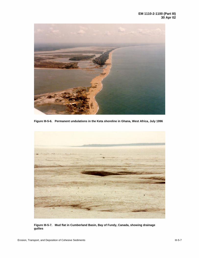
EM 1110-2-1100 (Part III)30 Apr 02
Erosion, Transport, and Deposition of Cohesive Sediments III-5-7
Figure III-5-6. Permanent undulations in the Keta shoreline in Ghana, West Africa, July 1996
Figure III-5-7. Mud flat in Cumberland Basin, Bay of Fundy, Canada, showing drainagegullies

EM 1110-2-1100 (Part III)30 Apr 02
III-5-8 Erosion, Transport, and Deposition of Cohesive Sediments
Figure III-5-8. A mud ‘beach’ backed with eroding salt marsh at Annapolis Royal, in theAnnapolis Bay of the Bay of Fundy. Basalt revetment at top of salt marsh is an attempt to halt the erosion
(3) Mangrove. Tropical coastal wetland where the vegetation, in the form of trees, can withstandrelatively severe wave attack (Figure III-5-9). Depth-limited waves will penetrate a mangrove, eroding mudfrom around the root system in extreme storms, and endangering individual trees. Mangrove can be foundbetween mud flats and salt marsh, and can transmit waves, which erode the adjacent salt marsh behind it.
(4) Mud ‘beach.’ A sloping mud shore, exposed to wave attack often following the destruction ofmangrove or other wetland vegetation (Figure III-5-8). The usual cause of wetland or mangrove destructionis property developers, municipal agencies, and individuals wishing to ‘reclaim’ the shore. Naturaldestruction occurs from the seaward edge, through undermining of the root system by waves and currents.
III-5-3. Erosion Processes on Consolidated Shores
a. Erosion processes on cohesive shores are distinctly different from those on sandy shores. There arealso differences between consolidated and mud cohesive shores. On consolidated shores, the erosion processis irreversible because, once eroded, the cohesive sediment (e.g., glacial till, glacio-lacustrine deposits, icebonded sediments, soft rock or other consolidated deposits) cannot be reconstituted in their consolidated formin the energetic coastal environment. Furthermore, since the sand and gravel content is low in these deposits(often less than 20 percent), erosion is not balanced by an equal volume of deposition within the littoral zone.The eroded fine sediments (silt and clay) are winnowed, carried offshore, and deposited in deep water incontrast to the sand fraction, which usually remains in the littoral zone.

EM 1110-2-1100 (Part III)30 Apr 02
Erosion, Transport, and Deposition of Cohesive Sediments III-5-9
Figure III-5-9. Sand beach disappearing into mangrove on the island of Borneo. Sediment withinthe mangrove is cohesive mud
b. Consolidated cohesive sediment is eroded by at least four mechanisms:
(1) Through abrasion by sand particles moved by waves and low currents.
(2) Through pressure fluctuations associated with turbulence generated at various scales such as wave-breaking-induced turbulence that reaches the lake or seabed and large-scale eddies that may develop in thesurf zone.
(3) Through chemical and biological influences.
(4) Through wet/dry and freeze/thaw cycles where exposed to the atmosphere.
c. Sand can also provide a protective cover to the underlying cohesive substratum. However, only whenthe sand cover is sufficient to protect the cohesive substratum at all times will the shore revert to a sandyclassification (i.e., truly a ‘thick pile of sand’).
d. On consolidated cohesive shores, the rate of lake or seabed downcutting determines the long-termrate at which the bluff or cliff retreats at the shoreline. In other words, while subaerial geotechnical processesmay dictate when and where a slope failure will occur, the frequency of failures over the long term isdetermined by the rate at which the nearshore profile is eroded (i.e. the downcutting rate). Subaqueous andsubaerial erosion processes on cohesive shores are discussed in detail in Part III-5-7. In addition, thegeomorphology of cohesive shores and the relationship to erosion processes is the topic of Part III-5-5.
EM 1110-2-1100 (Part III)30 Apr 02
III-5-10 Erosion, Transport, and Deposition of Cohesive Sediments
III-5-4. Physical and Numerical Modeling
a. Laboratory or physical model experiments have been used in two ways: (1) to improve theunderstanding of the fundamental principles of cohesive shore erosion processes, and (2) to develop ameasure of the erodibility of specific samples of cohesive sediment.
b. In the former category, scale model tests have been performed in wave flumes as described bySunamura (1975, 1976 and 1992) for erodible rocky coasts similar to consolidated cohesive behavior, byNairn (1986) for a section of the Lake Erie shoreline using an artificial clay, and by Skafel and Bishop (1994)and Skafel (1995) using intact samples of till removed from the Lake Erie shoreline. The tests described bySkafel and Bishop (1994) included an assessment of the relationship between wave properties (e.g.,wave height, orbital velocity, type and fraction of broken waves) and local erosion rate and therelationship between sand cover and erosion rates. Laboratory experiments on erosion and deposition ofmud are described in Part III-5-6c(9). The annular flume, used in both the laboratory and the field (e.g.,Amos et al. 1992, Krishnappan 1993) may be regarded as a full-scale model of the response of a mud bed toshear.
c. The primary difficulty in the use of physical model experiments of cohesive shores is the scaling ofthe cohesive material. At present, it is not possible to accurately scale cohesive sediment with respect toits erosion resistance properties. Therefore, model tests must be interpreted qualitatively, or full-scale testsmust be conducted using low wave energy conditions. Nevertheless, the noted tests have been extremelyvaluable in advancing the understanding of cohesive shore erosion processes both inside and outside the surfzone.
d. A technique of assessing the erodibility of intact samples of consolidated cohesive sediment inunidirectional flow conditions has been developed and applied by Kamphuis (1990), and, more recently, forthe assessment of cohesive sediment samples removed from the southeast shoreline of Lake Michigan(Parson, Morang, and Nairn 1996). These tests are typically performed for both clear water and sand in flowconditions to elucidate the importance of sand as an abrasive agent. This approach for defining the erodibilityof cohesive sediment samples is discussed in more detail in Part III-5-7b.
e. The development and application of numerical models for describing erosion processes on cohesiveshores is not far advanced owing to the complexity of the processes involved. Most numerical models maybe described as little more than numerical frameworks for interpolating or extrapolating observed behaviorof cohesive sediments in water. Essentially, a numerical model of cohesive shore erosion must define thenear-bed flow conditions within the surf zone, the movement of any overlying noncohesive sediment cover,as well as the erosion resistance properties of the cohesive sediment (which change with time due to exposureof sediment layers and subaerial drying). Numerical modeling of cohesive shores is summarized inPart III-5-12.
f. The best 3-D numerical mud models (e.g. Le Hir 1994) treat the water column as a continuum: fromstationary consolidating bed, through fluid mud, to sediment maintained in suspension by turbulence. Thereare nevertheless bed sediment ‘modules,’ which use the equations presented in Parts III-5-7, 9, and 10 tocalculate erosion and deposition, supplying sediment and new bathymetry to numerical hydrodynamic modelsthat transport the sediment by advection and dispersion (Part III-5-8a).
g. All mud models need to track sediment layering - the composition and state of each sediment layerat each grid point in the model — more a bookkeeping function than numerical modeling.
EM 1110-2-1100 (Part III)30 Apr 02
Erosion, Transport, and Deposition of Cohesive Sediments III-5-11
h. Part III-5-13 provides some detailed guidance on the specific coastal engineering and managementissues associated with cohesive shores. The success of engineering and management techniques on cohesiveshores is dependent on a recognition of the fundamental differences between sandy and cohesive shoreprocesses. Engineering techniques that may have been successful on the more familiar sandy shores, maybe unsuitable or inappropriate along cohesive shores.
III-5-5. Geomorphology of Consolidated Shores
This section provides a review of the geomorphology of cohesive shores and the relationship between the landforms and the erosion processes discussed in the previous sections. The discussion is subdivided under twoheadings: “Controlling Factors” and “Profile Types.” This section focuses on the geomorphology ofconsolidated cohesive sediment shores. For more detail on erosion processes along rocky coasts, refer toSunamura (1992).
a. Controlling factors. The primary controlling factors discussed in the following paragraphs influencethe geomorphology of cohesive shores:
(1) Lag deposits.
(a) Some consolidated cohesive sediment units have cobbles or boulders within their composition. Forexample, along the Great Lakes, glacial till may be either fine-grained or stony (i.e., containing gravel andcobbles). During the evolution of stony till shores, the cobbles and boulders that are left behind after theremoval of the finer clay, silt, and sand build up to form a protective armor for the underlying till. In thesecases, an erosion-resistant nearshore shelf will usually have formed. The depth of the shelf at any locationis such that the lag deposit remains immobile, and therefore the depth is determined by the local wave climateand the grain size of the lag deposit. Generally, for the Great Lakes, the depth of this shelf is approximately2 m below low water datum. Along sea and ocean coasts with large tidal ranges and longer waves, lagdeposits may occur at much greater depths (e.g., lag deposits over clay have been found in water depths of10 m below datum along the North Sea coast of England). The shelf creates what has been referred to as aconvex profile, in contrast to the concave profile associated with situations where lags are not present.
(b) The armored shelf acts to dissipate wave energy, and therefore reduce or even prevent bluff erosion.Boyd (1992) gives several examples where a bluff is protected from erosion by a nearshore shelf and notesthat the reduced wave energy may also allow a stable beach to exist at the shore, providing additionalprotection to the bluff toe. Natural headlands along an eroding cohesive shoreline often owe their existenceto the presence of a lag-protected nearshore shelf.
(c) An example of a site where a lag deposit has resulted in an erosion-resistant foreshore and a stableshoreline is located near the town of Goderich on the Canadian shore of Lake Huron. A nearshore profilefor this site is shown in Figure III-5-10. The cobble-protected shelf has a depth of 1.75 m and is about 200 mwide. The stratigraphy at the site consists of a stony till unit below the average lake level and a fine-grainedtill unit above the average lake level. At nearby sites where the fine-grained till unit dips below the averagelake level to depths of greater than 2 m, and the nearshore shelf is no longer present, the bluff recession ratesrange from 0.3 m/year to over 1 m/year.
(2) Different stratigraphic units.
(a) Along most cohesive shores, 3-D variations in contact surfaces between stratigraphic units arecommon. This results from the complex geomorphologic conditions that formed the underlying geology,which, depending on the location, may include some combination of: glacial, lacustrine, estuarine, or fluvial

EM 1110-2-1100 (Part III)30 Apr 02
III-5-12 Erosion, Transport, and Deposition of Cohesive Sediments
Figure III-5-10. A convex consolidated cohesive profile with a shelf protected by lag deposits located nearGoderich, Ontario, on Lake Huron
processes. Therefore, as the shore erodes in time, the recession rates can change, as either more or lesserosion resistant, units are encountered further inland. One example of the influence of erosion resistanceis East Point located along the Scarborough Bluffs east of Toronto on Lake Ontario. The plan andstratigraphy cross section of this feature are shown in Figure III-5-11. Clearly, East Point is an expressionof the more erosion-resistant Leaside (or northern) till unit, which dips below the average lake level at thislocation. Leaside till is relatively hard and includes boulder pavements (Boyce, Eyles, and Pugin 1995).Along the neighboring shore, the less erosion-resistant Scarborough clay unit exists below the lake level.
(b) Recognition of the variation in erosion resistance of different till units resulted in an unlikely findingduring the investigation of the influence of a harbor structure at Port Burwell on downdrift erosion along thenorth central shore of Lake Erie (Figure III-5-12). A long harbor jetty here intercepts almost all of the sandmoving along the shore from west to east, therefore depriving the downdrift shore of sediment. On a sandyshore, this would be a clear case of downdrift erosion due to sediment supply starvation. However, theinvestigation described by Philpott (1984) revealed that cohesive shores along the north central shore of LakeErie seldom have (and probably never had) enough sand to halt the downcutting of the underlying till.Updrift of the harbor, the trapping of large quantities of sand eventually halted the nearshore profiledowncutting, and the bluff position was stabilized. However, this still did not fully explain why recessionrates updrift of the harbor fillet beach were generally lower (about 1 m/year) than those on the downdriftshoreline to the east (in the range of 2 to 4 m/year).
(c) Figure III-5-12 also describes the bluff face stratigraphy at Port Burwell. There is a change in thesubaqueous stratigraphic unit at the harbor mouth, where Port Stanley till exists below the lake level on theupdrift side and Waterlain till forms the nearshore profile on the downdrift side. Based on a comprehensiveinvestigation, including laboratory testing of the erodibility of the different till units, it was concluded thatWaterlain till was less erosion-resistant than the Port Stanley till. It is not coincidental that the change in till

EM 1110-2-1100 (Part III)30 Apr 02
Erosion, Transport, and Deposition of Cohesive Sediments III-5-13
Figure III-5-11. Plan and cross section of East Point along the Scarborough Bluffs (located east of Torontoon Lake Ontario) showing the influence of the erosion-resistant leaside (or northern) till on the localgeomorphology
occurred at the harbor mouth, as often creeks or rivers follow the interface between different stratigraphicunits.
(d) Riggs, Cleary, and Snyder (1995) provide several examples of both headlands (local areas of slowlyretreating or stable shoreline) and local sections of rapidly retreating shoreline, that are a direct result ofvariability in the erosion resistance of different stratigraphic units that make up the shoreface. They foundthat headlands result from the presence in the nearshore of more erosion-resistant Pleistocene or oldersediments. In contrast, rapidly retreating sections of shore consisted of sand-poor, valley-fill sediment orcompact peats and clays deposited in modern estuarine environments.
(3) Quantity and mobility of sand cover.
(a) In natural situations, a protective sand cover can build up over an erodible substrate and protect itfrom further erosion. Investigations of Great Lakes sites have shown that approximately 200 m3/m of sandcover (measured from the top of the beach out to the 4-m contour) is required to halt the downcutting process(Nairn 1992). However, even half as much as this quantity can afford at least some protection to theunderlying cohesive substratum.
(b) Another important factor is the volatility or mobility of sand cover. If the overlying noncohesive bedforms are rapidly and frequently changing position, the underlying cohesive substratum will be exposed toerosive situations more frequently. Nairn and Parson (1995) have indicated that on the Great Lakes, the shiftof bar position in response to changing lake levels has an important influence on the exposure of theunderlying till (in the troughs between the bars) to erosion. On an eroding cohesive bluff shore along theNorth Sea coast of England, Pringle (1985) identified alongshore migrating areas of reduced beach cover andexposed glacial till called ‘Ords.’ These Ords have an important role in exposing the underlying glacial tillto erosion. Figure III-5-13 shows an Ord on the Holderness coast at low tide with glacial till exposed (partly

EM 1110-2-1100 (Part III)30 Apr 02
III-5-14 Erosion, Transport, and Deposition of Cohesive Sediments
Figure III-5-12. Plan and cross section of the Port Burwell area on the north central shore of Lake Erieshowing the influence of a fillet beach and stratigraphy changes on the geomorphology of a cohesive shore
covered with cobbles) between the upper coarse sand beach and a bar consisting of finer sand. The closeupphoto of the Ord (Figure III-5-14) shows erosion of the exposed till around a 10-cm-high pedestal protectedby a rock cap. Pringle (1985) found that the migration rate for these features was approximately 500 m/year,which is similar to the rate of migration for large sand waves or rhythmic features along Long Island, NY(Thevenot and Kraus 1995). An Ord could be defined as the area between two migrating sand waves. Insummary, both cross-shore and alongshore variations in sand cover thickness resulting from migration of barsand sand waves or Ords, respectively, have an important influence on the rate of cohesive sediment erosionin the nearshore zone.
(c) Deposition of large quantities of sand over a cohesive substrate can occur at a change in shorelineorientation where the potential alongshore sediment transport rate rapidly decreases, or at a naturalobstruction to alongshore transport, such as at a rock headland. Other instances where sand may eventuallybuild up to protect a profile include sites where the alongshore transport of sediment is intercepted at a harborjetty. The Port Burwell fillet beach shown in Figure III-5-6, as discussed above, protects the nearshorecohesive substratum and has stopped the bluff recession behind the fillet beach.

EM 1110-2-1100 (Part III)30 Apr 02
Erosion, Transport, and Deposition of Cohesive Sediments III-5-15
Figure III-5-13. Bluff erosion along the Holderness coast of the North Sea. The underlyingcohesive profile is exposed at low tide in a trough (referred to as an “Ord”) between the upperbeach and first bar
Figure III-5-14. Close-up of the exposed cohesive profile on the Holderness coast (Figure III-5-13). A rock-capped pedestal of cohesive sediment, about 10 cm in height, has developed througherosion of the adjacent seabed

EM 1110-2-1100 (Part III)30 Apr 02
III-5-16 Erosion, Transport, and Deposition of Cohesive Sediments
Mean lake level
Initial sand veneer
Bars
ConcaveProfiles(typical)
ConvexProfiles(typical)
Beach deposit
Cobble/boulder lag deposit
Mean lake level
Figure III-5-15. Distinctions between concave and convex consolidated cohesiveprofiles
(d) Many areas along the Great Lakes shores that once had sufficient sand cover to protect an underlyingcohesive substratum from downcutting are now coming under attack as the sediment supply has been reducedthrough human influences. Reductions to the sediment supply occur through entrapment of sediment atstructures which protrude into the lake (including harbor jetties and land reclamation projects that have beencreated for many purposes, such as power plants, marinas, and docking facilities) as well as throughprotection of previously eroding sections of shoreline. Shabica and Pranschke (1994) describe one such areanorth of Chicago on Lake Michigan where the sand cover has decreased from 560 m3/m in 1975 to 190 m3/min 1989. If the depletion of sediment cover continues at this site, the previously very low rates of shorelinerecession (less than 0.2 m/year, or 8 in./year) may accelerate.
(4) Local wave and water level conditions. The characteristics of the local wave and water levelconditions represent the fourth controlling factor on the geomorphology of consolidated cohesive coasts.Both the intensity and the directionality of the waves can influence the rate of erosion at a particular shoresite. Other factors being equal, greater wave energy translates to higher downcutting rates and more rapidshoreline erosion. Directionality of the waves can have a secondary influence on downcutting rates byaffecting the mobility of the sand cover over the underlying till. Large swings in wave direction can resultin a more dynamic system with respect to the sediment cover. Fluctuations in water level also have animportant role in cohesive shore erosion processes as explained by Stewart and Pope (1993) andFuller (1995). While direct erosion at the bluff toe may be accelerated during high-water conditions, lowwater leads to acceleration of the nearshore downcutting process (which in turn allows more waves to reachthe bluff toe).
b. Profile types. Boyd (1981, 1992) completed an extensive review of nearshore profile shapes forconsolidated cohesive shores on the Great Lakes. These essentially fall into two categories: concave profilesand convex profiles. Figure III-5-15 provides a schematic description of these two profile types.

EM 1110-2-1100 (Part III)30 Apr 02
Erosion, Transport, and Deposition of Cohesive Sediments III-5-17
(1) Concave profiles. Concave profiles develop in fine-grained sediment with a relatively uniformerosion resistance from the closure point up to the top of the bluff or cliff. These profiles have an exponentialform similar to sandy shore profiles described by Dean (1977). Sand cover over these cohesive profiles canrange from perhaps as little as 25 to over 200 m3/m measured between the bluff toe and the 4-m depthcontour. The sand cover can be in the form of bars, and, in areas with a sand cover in the high end of therange, a substantial beach at the shore. Stewart and Pope (1993) found that a reduction in the range of waterlevel fluctuations would not reduce the long-term erosion rates for cohesive shores with concave profiles.As explained above, lower water levels result in accelerated lowering of the nearshore profile, whichessentially has the same effect as high water levels — allowing waves to reach the bluff toe.
(2) Convex profiles. As noted above, convex profiles develop at locations where potential lag depositsexist within the eroding material. These profiles are characterized by a nearshore shelf, which on the GreatLakes has a depth approximately 2 m below low water datum. At other locations, this depth will bedetermined by the median grain size of the lag deposit, the wave climate, and the range of water levelfluctuations. Long-term erosion rates along these shores are less than rates for concave cohesive shores(having limited sand cover) with the same wave exposure. With the exception of high-water periods, theerosion-resistant nearshore shelf acts to dissipate wave energy before it reaches the shoreline. However,during high water periods, these shorelines are more vulnerable to erosion when waves are able to attack thebluff toe. Therefore, in contrast to cohesive shores with concave profiles, shores with convex profiles wouldbenefit from a reduction in the range of water level fluctuations (Stewart and Pope 1993). Finally, the fishhabitat function of cohesive shores with a convex profile shape is much more important owing to the surficialsubstrate (cobbles and boulders with limited sand cover) and the proximity to a deepwater drop-off at the edgeof the shelf.
III-5-6. Sediment Properties and Measurement Techniques
a. Introduction.
(1) In the case of noncohesive sand and gravel, sediment mobility can be estimated just by knowing thegrain size and shape, specific gravities of the sediment and water, and the viscosity or temperature of thewater (i.e., physical properties). The mobility of cohesive sediment is a more complex phenomenon.Cohesion (particle attraction) is governed by the electrochemistry of the sediment mineral and water; its stateof consolidation; and in many cases, by the presence of organisms like diatoms, which can bind the sedimentparticles together with mucus.
(2) The extent of data requirements will vary depending on the nature of the coastal engineering problemand the nature of the shore. This section presents an overview of the range of possible field and laboratoryinvestigations that can be used to characterize the conditions associated with erosion, transport, deposition,and consolidation on a cohesive shore. This discussion focuses on a characterization of the specific geologicconditions related to the cohesive shore. For the measurement of environmental conditions (e.g., waves andwater levels), refer to Part II-3.
b. Consolidated shore erosion. Developing an understanding of consolidated shore erosion requiresinformation on profile shape (beach and nearshore profile techniques are summarized in Part III-3-2),presence or absence of lag deposits, bluff and nearshore stratigraphy, erodibility of the one or more cohesiveunits in the active nearshore erosion zone (i.e., between high water and the depth of closure), and the sandcover thickness and stability. Available techniques to assess the characteristics listed above are as follows:

EM 1110-2-1100 (Part III)30 Apr 02
III-5-18 Erosion, Transport, and Deposition of Cohesive Sediments
(1) Field sampling and geotechnical analyses.
(a) Testing may be performed in situ or in a laboratory on samples extracted from the field. Extractiontechniques for seabed or lake bed cohesive sediments include: dredging; coring; box coring; and cuttingsamples (the latter using a chainsaw with a trenching chain). As noted in Part III-5-6, it is important toretrieve intact samples that, to the extent possible, preserve the natural structure of the cohesive sediment.
(b) None of the available standard geotechnical test procedures provide a direct measure of the erosionresistance of a cohesive sediment in the coastal environment. Nevertheless, the more important characteristicsthat provide an indirect assessment of erodibility include: grain size analysis (including clay content); liquidand plastic limits; water content; undrained shear strength; bulk density; and consolidation pressure.Techniques for establishing these parameters are presented in the USACE Engineering Manual “LaboratorySoils Testing” (EM 1110-2-1906). Undrained shear strength can be determined in the field using a conepenetrometer or a vane shear apparatus.
(c) Borehole information can be valuable for assessing variations in stratigraphy both above and belowthe water level.
(2) Laboratory erodibility experiments.
(a) There are no standard and accepted approaches for establishing the erodibility of cohesive sedimentin the coastal environment based on geotechnical properties. Therefore, to quantify the relationship betweenerodibility and shear stress applied under a given flow condition, it is usually necessary to perform laboratoryexperiments. Experiments may not be required where direct techniques have been applied to determine theerodibility of similar sediment. It is advisable that these experiments be performed with intact, and to theextent possible, undisturbed samples of cohesive sediment in order to preserve the natural structure of the soil.
(b) Four laboratory techniques for assessing erodibility are briefly reviewed in this section. Theseprovide an example of the range of techniques that are available.
(c) Arulanandan, Loganatham, and Krone (1975), and more recently Zeman (1986), describe the use ofa rotating cylinder apparatus to assess the erodibility of intact and undisturbed samples of cohesive sediment.This technique is also mentioned for testing the erodibility of mud. In this approach, a long cylindricalsample is mounted inside a larger transparent cell. The cell is then filled with water and rotated. Duringrotation, the torque transmitted to the inside stationary cylinder is measured to quantify the shear stressapplied to the sample. At the end of the test, erosion rates are determined by the loss in mass of the sample.A disadvantage of this approach is the inability to introduce sand to the flow to assess the important influenceof sand abrasion.
(d) Another small-scale laboratory technique for testing intact and undisturbed samples is described byRohan et al. (1986). This procedure is based on an adaptation of the standard pinhole test. Water is circulatedthrough a hole drilled through the axis of a cylindrical sample. The head loss caused by friction in the sampleis measured using differential manometers in order to assess the shear stress applied to the soil by the flow.Depending on the size of the hole bored in the sample, it is possible that this technique could be adapted toassess the influence on erosion of sand in the flow.
(e) At a larger scale, intact and undisturbed cohesive sediment samples can be placed in a drop sectionin the floor of a unidirectional flow flume or tunnel. The sample is then exposed to different flow conditionswith and without the presence of sand, and the erosion of the sample surface is surveyed intermittently todetermine erosion rates for the different conditions. This technique is also frequently used for mud.Kamphuis (1990) describes the use of a tilting tunnel in which Pitot tubes were used to determine a velocity

EM 1110-2-1100 (Part III)30 Apr 02
Erosion, Transport, and Deposition of Cohesive Sediments III-5-19
Figure III-5-16. Laser doppler velocimeter (LDV) used to determine shear stress exerted on the tillbed in a unidirectional flow flume test. This test features sand in the flow acting as an abrasive
profile upstream and downstream of the sample in order to determine the shear stress applied to the sampleby the flow. Cornett, Sigouin, and Davies (1994) describe a similar approach using a tilting flume for theanalysis of samples extracted from the bed of Lake Michigan near St. Joseph Harbor (Parson, Morang, andNairn 1996). In this case, a laser doppler velocimeter measured the velocity profile near the bed in order toestablish the shear stress applied to the sample by the flow (Figure III-5-16). This figure shows a sand veneermigrating over the till sample in the unidirectional flow flume. In both the Kamphuis (1990) and the Cornett,Sigouin, and Davies (1994) tests, the maximum flows generated were in the range of 3 to 3.5 m/sec (10 to12 ft/sec). Results from experiments using this technique to estimate erodibility are presented in Part III-5-7b.
(f) The most realistic approach that can be taken to assess erodibility in a laboratory setting is to createa nearshore profile with intact and undisturbed cohesive sediment samples in a wave flume or basin. Thisapproach was used by Skafel and Bishop (1994) to complete important research into the erosion processeson cohesive shores. Intact samples, measuring 1 m by 0.35 m by 0.45 m, encased in an open-ended steel boxwere extracted from the top of a bluff on Lake Erie and placed directly in a wave flume. The open-endedsteel box was pushed slowly into the till by a 20-ton hydraulic ram and the till at the inner end of the box wascut away using a chainsaw with a trenching chain. The box was then removed with a crane. The till boxeswere installed in the flume to create the desired profile shape. In these tests, the effects of sand cover in theform of migrating bars or a patchy veneer were tested. Also, the influence of breaking waves on the erosionof the cohesive sediment was assessed.
EM 1110-2-1100 (Part III)30 Apr 02
III-5-20 Erosion, Transport, and Deposition of Cohesive Sediments
(3) Field techniques for assessing surface and subsurface conditions.
(a) One of the most important pieces of information in characterizing a cohesive shore profile is the sandcover thickness across the underlying cohesive profile (i.e., measured from the bluff toe out to a depth of atleast 4 m). In addition, where the cohesive profile is exposed, it is also important to determine whether ornot a protective lag deposit exists. As with any coastal engineering site investigation, beach and nearshoreprofiles are essential information. In this section, a variety of techniques for characterizing the surface andsubsurface conditions, with particular focus on the sand cover thickness, are presented, ranging from thesimplest to the most sophisticated.
(b) The simplest technique of estimating the thickness of the sand cover across the profile involves thefollowing tasks:
• Complete a beach and nearshore profile from the toe of the bluff out to the depth of closure (betweenthe 5- and 10-m water depth).
• Through the use of a steel probe or test pits, attempt to determine the thickness of sand cover nearthe waterline.
• Estimate the shape of the underlying cohesive profile (as a smooth exponential form) joining pointsbetween the toe of the bluff, the position of the till at the waterline (if determinable), and the troughs betweenthe bars on the profile. Typically, the till will be exposed or only thinly covered in the troughs. If repeatedprofiles are available at a site, these may provide additional information on the position of the underlying tillif the position of the troughs between bars shifts between surveys.
(c) In order to complement the simple technique described above, a diving inspection could be completedacross the profile. The diver could use an underwater video to document conditions, and a steel probe toestimate sand cover thickness at different locations. Depending on the extent of sand cover, the till may beexposed in some areas. Alternatively, a frame-mounted video camera lowered from a boat or a remotelyoperated vehicle with video could be used. Video is also valuable in assessing whether or not a lag depositexists where the cohesive layer is exposed.
(d) In place of a simple steel probe, a jet probe could be used to survey the thickness of the sand coveron the land and underwater. A jet of either water or air can be used to penetrate the sand cover (the latter isonly applicable underwater). Shabica and Pranschke (1994) describe the use of a hydraulic probe consistingof an extendible 20 mm diameter pipe through which water is pumped at 2.8 kg/cm2 (40 psi).
(e) A technique based on electrical resistivity has been used to establish the sand thickness across thesubaerial section of beach for sections of the Holderness shoreline. This method is particularly useful atlocations with large tidal ranges that allow for significant sections of the profile to be surveyed at low tide.
(f) Ground-penetrating radar was used to survey the thickness of the sand cover for several profilesdowndrift of St. Joseph Harbor (Parson, Morang, and Nairn 1996). The limitation of this technique is thatit can only be used in a freshwater environment.
(g) Sub-bottom profiling, or high-frequency seismic imaging, is another geophysical technique that iscapable of establishing the thickness of sand cover over an underlying cohesive profile. Side-scan sonar isan acoustic technique that provides an image of the seabed or lake bed surficial conditions. While thisprocedure would not be capable of determining the thickness of sand cover, it could provide useful surficialinformation such as the extent of exposed gravel and cobble lag deposits. These methods are described inPart IV-5 in greater detail.

EM 1110-2-1100 (Part III)30 Apr 02
Erosion, Transport, and Deposition of Cohesive Sediments III-5-21
c. Erosion, transport, and deposition of mud. In the case of mud, it is useful first to examine thefollowing hydrodynamic sediment properties that will be required by the equations presented later:
(1) Cohesion. The cohesive bond is predominantly electrochemical, increasing with the electricalconductivity of the ambient water and proximity of the particles. Conductivity increases with salinity. Thebond between particles may be enhanced, particularly at rest on the bed, by biological ‘glues’ such as themucus excreted by diatoms, worm tubes, and feces (Paterson 1994).
(2) Critical shear for erosion.
(a) As water flows over the mud bed, as either steady flow or oscillatory flow under tides and waves, itexerts a shear stress τ on the bed due to viscosity and turbulence (described in greater detail in Part III-6).Not only is shear a real physical stress on the bed sediment, but it also serves as empirical shorthand for thelevel of turbulence in the flow. Thus, it is a useful parameter in describing suspended load sedimenttransport; as well as fluid mud (bed load), erosion, and deposition.
(b) At the level of a stationary particle on the bed, shear forces are balanced by the forces of gravity,interparticle friction, and cohesion. Shear is augmented by lift and drag, making the force balance
SHEAR + LIFT + DRAG < GRAVITY + FRICTION + COHESION
a vector sum, the same as that for noncohesive sand and gravel, but with the addition of cohesion. As flowincreases, the left-hand side of this balance increases approximately as the square of velocity, until
SHEAR + LIFT + DRAG = GRAVITY + FRICTION + COHESION
and the formerly stationary particle leaves the bed and begins to move. The shear stress at which this occursis known as the critical shear for erosion or erosion threshold τc. τc is still shorthand for the entire left-handside of the balance, not shear alone.
(c) The sediment ‘particle’ may be an individual grain; but more likely a floc, made up of several grainsheld together by cohesion. Cohesion plays the major role in the right-hand side of the force balance, andfailure (erosion) will occur where cohesion is weakest.
(d) Critical shear τc is not a particularly useful concept in fluid mud. At the water/fluid mud interface,the applied shear stress is balanced by a shear strain (flow) of the fluid mud, rather than GRAVITY + FRICTION + COHESION. Also, the fluid mud is essentially a thick, viscous, laminar, boundary layer,protecting the stationary bed from any SHEAR + LIFT + DRAG approaching τc. Erosion of fluid mud isbetter described by densimetric Froude Number entrainment between two fluids (Part III-5-7e).
(3) Erosion rate at twice critical shear. Both the Parthenaides and Krone Equations (Parts III-5-7d andIII-5-9c) are ‘excess shear’ fits to observed erosion and deposition, respectively. For example, theParthenaides Equation (Part III-5-7d) correlates observed erosion rates with
Dimensionless Excess Shear = (τc - τ) / τc; negative (τc < τ) for erosion
The Parthenaides coefficient Mp (in units of kg/m2/sec) (see Equation III-5-1), is the correlation coefficientbetween erosion rate and excess shear, when dimensionless excess shear = -1; that is, when τ = 2τc.
(4) Critical shear for deposition.
(a) A critical shear stress for deposition τs Pa (lbf/ft2) is not obvious at first glance. In noncohesivesediment, the critical shear for deposition is only slightly less than that for erosion: a noncohesive particle
EM 1110-2-1100 (Part III)30 Apr 02
III-5-22 Erosion, Transport, and Deposition of Cohesive Sediments
will come to rest almost as soon as the shear is too small to move it. But the process of deposition of cohesivesediment flocs is quite different; τs is generally on the order of one fourth of τc.
(b) High shear near the bed breaks up large flocs before they can settle. Then, the resulting smaller flocsand individual particles are resuspended. The critical shear for deposition τs is that through which large flocscan pass without being broken up. Note that τs is not shorthand for something more; τs really is the shearstress in the bottom boundary layer which cannot overcome cohesion in the settling flocs.
(5) Sediment, fluid mud, and water densities.
(a) Important densities and specific gravities:
ρw = specific gravity (mass density) of water — 1,000 kg/m3 (62.4 lb/ft3) in fresh water, up to1,030 kg/m3 (64.3 lb/ft3) in seawater
ρs = specific gravity (mass density) of sediment mineral (no voids): generally 2,000 kg/m3 (125 lb/ft3)to 2,700 kg/m3 (170 lb/ft3) depending on mineral
(b) Bulk sediment density voids filled with ambient water:
• Of freshly deposited flocs (may be fluid mud if < 1,100 to 1,200 kg/m3 (70 to 75 lb/ft3),corresponding to a mass concentration in excess of about 20 kg/m3 (20 ppt)).
• Of existing bed surface, and layers, e.g., 1,400 kg/m3 (90 lb/ft3).
• Of fully consolidated sediment, generally < 2,000 kg/m3 (125 lb/ft3).
(6) Grain size and settling velocity.
(a) Settling velocity is a more important hydrodynamic property of cohesive sediment than grain size.Settling velocity is a measure of the sediment’s behavior in suspension; grain size only allows us to guess thesettling velocity.
(b) The first thing to know about cohesive sediment grain size is that it is not a measurable physicalconstant. True, the size of individual dispersed grains may be inferred from measurements of their settlingvelocities in distilled (free of dissolved chemicals) water: generally on the order of 10-µ or less. The settlingvelocity of a 10-µ sphere, 2,500 kg/m3 (156 lb/ft3), in water of 20 EC (68 EF) is 0.06 mm/sec (0.002 in./sec).
(c) But cohesive sediment of this size in natural, often salt, water does not stay dispersed for long.Grains stick together when they come close enough for the cohesive forces to overcome the fluid shear andgravity keeping them apart. Aggregations of cohesive sediment grains are called ‘flocs.’ Flocs are larger thanindividual grains, of course, but because of water trapped within the floc, they are also less dense than

EM 1110-2-1100 (Part III)30 Apr 02
Erosion, Transport, and Deposition of Cohesive Sediments III-5-23
the pure mineral. Depending on the relationships among floc size, shape, and density, the result is a flocsettling velocity that may be more or less than that of individual grains. The settling velocity must bedetermined with the natural sediment in the natural water.
(d) Mud may also be biologically cohesive (Paterson 1994), for example, due to mucus excreted bydiatoms. Biological cohesion is even more difficult to predict than electrochemical, providing yet anotherreason for using natural sediment and natural water in determining floc size and settling velocities.
(7) Degree of consolidation.
(a) The degree of consolidation u is defined as the ratio of the bulk density of the sediment to the bulkdensity of the ‘fully consolidated’ sediment, measured under Part III-5-6b(5). Consolidation of cohesivesediment is the compaction of the soil mass accompanied by drainage of the interstitial water, just as withnoncohesive sediment. The principal difference is the length and cross-sectional area of the drainage path.In cohesive sediments, the path length is long and the area is small (i.e., low permeability); slowing downdrainage and consolidation. Drainage is through the bed surface, into the ambient water, so that a goodrelative measure of the length of the drainage path P is the depth of burial below the surface. Cross-sectionalarea of the drainage path must be inferred from measurements of permeability.
(b) Overburden speeds up consolidation but increases the length of the drainage path, especially whenthe overburden is also cohesive. Nevertheless, consolidation starts at the bottom of a sediment layer andfollows the draining water upward, giving even a freshly deposited layer a density gradient, denser at thebottom to less dense at the surface, until the entire layer is fully consolidated. The strength of the sedimentrepresented by the critical shear for erosion τc increases with density and consolidation.
(8) Field measurement techniques. Many of the cohesive sediment field and laboratory measurementtechniques are the same as those for noncohesive sediment (Part III-1). Nevertheless, some accommodationmust be made for mud:
(a) Bed sampling. Much depends on knowledge of the composition and density of surficial sediments,which can be gained from laboratory analysis of surface samples obtained in the field. It is unreasonable toexpect that undisturbed mud samples can be collected. In fact, it is difficult to contain most surficial mud inthe commonly used Shipek or Ponar grab samplers because the samples leak out. Underwater samples mayhave to be obtained by divers, and all samples that include entrapped water should be transported in sealedjars and stored at 4 EC (39 EF).
(b) Boreholes and cores. The techniques give information on subsurface sediment layers. Blow countsand cone penetration tests give a relative measure of the strength and density of the layers (but not of thecritical shears for erosion and deposition of mud, see below), and cores taken from the layers are as close toundisturbed samples as is possible in cohesive sediment. Boreholes should extend to bedrock or similar hard,impenetrable layers, with cores and cone penetration tests in each major layer.
(c) Suspended sediment sampling. This type of testing is needed to determine composition and quantityof sediment in suspension. Generally, the technique is to pump and filter 4 L of suspension and transport thefilter and contents to the laboratory for subsequent analysis. Alternatively, 1 L of suspension may be sealedin jars and transported to the laboratory for filtering and analysis there; this liter may be obtained by pumpingor from any of the proprietary suspension samplers. Filters should be no larger than 10 microns. Samplingshould be carried out at a minimum of four elevations over the depth, with special attention to the near-bedor fluid mud layer.

EM 1110-2-1100 (Part III)30 Apr 02
III-5-24 Erosion, Transport, and Deposition of Cohesive Sediments
(d) Settling tube. Field settling tubes, e.g., the ‘Owen Tube’ (Eisma, Dyer, and van Leussen 1994)measure the settling velocity of cohesive sediment flocs in ‘live’ natural water, even in a natural level ofturbulence. Typically an undisturbed sample of sediment-water suspension is captured in a horizontal tube.The tube is immediately turned into the vertical position, and the settling velocity of the flocs is determinedfrom density changes that occur in the suspension at various depths in the tube and over various times.
(e) Piezometers. These instruments measure rate of drainage of excess pore pressure from natural muds,and thus permeability and rates of consolidation. Lancelot (Christian, Heffler, and Davis 1993) is apiezometer that first creates excess pore pressure on its insertion in the mud bed, and then measures the rateof decay or drainage.
(f) Optical techniques. These techniques are primarily used as a substitute for suspended sedimentsampling. Two basic techniques are used: measuring light transmitted through a known illuminated volumeof suspension in a turbidity meter or transmissometer (e.g. Bartz, Zaneveld, and Pak 1978); or measuring lightreflected from the suspension by an ‘Optical Backscatterance (sic) Sensor’ or OBS (e.g. Sternberg, Shi, andDowning 1989). Both require calibration against natural sediment in known concentrations in natural water.
(g) Acoustic techniques. Many novel applications are still under development, mostly in the high-frequency (MHz) range, where for example, suspended sediment concentration and grain size profiles canbe measured (e.g. Hay and Sheng 1992). At lower frequencies, echo sounding detects the elevation of thebed and of the surface of fluid mud; and in the side-scan mode, detects bed forms such as ripples and dunes,and their orientation (Hay and Wilson 1994). At still lower (seismic) frequencies, sound penetrates the bedand detects the interfaces between sediment layers of different densities, creating sub-bottom profiles.
(h) Radioactivity techniques. In these techniques, Gamma rays or X-rays are passed through asediment/water suspension or bed layer (e.g. Sills 1994). The energy passing can be related by calibrationto the mass density of the suspension or layer. These techniques are particularly useful in characterizing fluidmud layers, as and where they occur. Radioactivity techniques are also used in laboratory consolidationcolumns.
(i) Direct shear techniques. There are several field devices that apply a variable shear stress to thesurface of a cohesive sediment bed (Gust 1994), and measure the variable rate of erosion (increase insuspended sediment in the water column) and deposition (decrease in suspended sediment in the watercolumn). Results can be used directly in the Parthenaides and Krone equations (Equations 5-1 and 5-4)respectively. The prototype for all such devices is the annular flume, described under Part III-5-6b(9)“Laboratory Measurement Techniques,” and sketched in Figure III-5-17. The Sea Carousel described byAmos et al. (1992) is an example of field adaptation of the annular flume.
(j) Correlation with shear strength. Although the critical shear for erosion τc would seem to be a functionof the shear strength of soft cohesive soil (measured by vane, cone, or penetrometer), the form of that functionis not yet known and certainly not linear. Even measuring mechanical surface shear directly on tidal mudflats (Faas et al. 1992) produces mechanical yield stress an order of magnitude larger than the hydrodynamicτc.
(9) Laboratory measurement techniques.
(a) Grain size analysis. Standard ASTM D422 laboratory techniques should be applied to determine thephysical size of individual grains in bed, core, and suspended sediment samples. Although no ASTMstandard has been published, the pipette technique (removing a known volume of suspension from a known

EM 1110-2-1100 (Part III)30 Apr 02
Erosion, Transport, and Deposition of Cohesive Sediments III-5-25
Figure III-5-17. Prototype direct shear device, the annular flume
elevation in the settling column, and filtering or drying to determine sediment concentration), is an alternativeto the hydrometer technique. Total dry weight of suspended samples is also required to give fieldconcentration in mg/l (ppm). Both hydrometer and pipette techniques measure settling velocity, and infergrain size from it. The settling column also measures settling velocity in the manner of a large-scale(typically greater than 1 m (40 in.) deep, 0.3 m (12 in.) diameter) hydrometer or pipette test (Gibbs 1972).Sensitive differential pressure transducers record the variations in suspended sediment concentration withdepth and time, from which settling velocity distribution in the sample can be computed. Like theconsolidation column below, settling columns need to be well-isolated from vibration and temperaturechanges to prevent artificial flocculation of the settling particles. For clay particules (<4 m), it will benecessary to use a nonstandard particle counter, e.g., Coulter counter. Nonstandard (natural water)hydrometer, pipette, or settling column tests should be used to estimate settling velocity of the flocs and bulkdensity of deposited sediment.
(b) Consolidation column. A consolidation column is a cylinder containing 2 to 3 m of natural sedimentand natural water in a vibration-free environment to ensure natural rates of consolidation (Sills 1994).Variations in pore pressure with time and depth (overburden) are measured with piezometers, and in density,with gamma ray or observed volume. Estimates of permeability (length and diameter of drainage paths, andvariation with bulk density) come out of the same measurements, using Equation 5-6, for example.
(c) Direct shear techniques. There are several laboratory devices that apply a variable shear stress to thesurface of a cohesive sediment bed and measure the variable rate of erosion (increase in suspended sedimentin the water column) and deposition (decrease in suspended sediment in the water column). Results can beused directly in the Parthenaides and Krone Equations of Parts III-5-7d and III-5-9c, respectively. Theprototype for all such devices is the annular flume (e.g., Krishnappan 1993), sketched in Figure III-5-17. Anannular flume is simply an endless channel in which the shear or velocity of rotation of the lid can be varied
EM 1110-2-1100 (Part III)30 Apr 02
III-5-26 Erosion, Transport, and Deposition of Cohesive Sediments
and the changes in the mud bed can be inferred from changes in suspended sediment concentration, measuredusing one of the techniques described above. The shear force driving the circulation can be measured directlyas the force needed to rotate the lid. Laboratory annular flumes generally rotate the flume and the lid inopposite directions, to minimize secondary radial circulation of the water, and to obtain a more uniformdistribution of shear on the mud bed. An increase in suspended sediment corresponds to a decrease in themass of sediment on the bed m and a decrease in suspended sediment to an increase in the mass of the bed.It is then possible to extrapolate these measured shear stresses to τc and τs, at which erosion or depositionceases; and to interpolate the Parthenaides coefficient Mp and fall velocity w (Example Problem III-5-1).
(10) Calibration techniques. Ideally, one should be able to measure all the hydrodynamic properties ofa cohesive sediment, and proceed directly to a model of the shore. The model, however, will always needcalibration and verification against measurements of erosion and deposition, to fine tune measurements andconfirm that the model represents the shore. With some of the hydrodynamic properties unknown, the modelcan be used to choose between high and low values of the unknown properties, using “design of experiments”techniques (Willis and Crookshank 1994). This still requires intelligent estimates of high and low values ofthe unknown properties and good field measurements of erosion, deposition, or transport.
III-5-7. Erosion Processes
a. Shear stress.
(1) The formulae for predicting the movement of cohesive sediment predict rates of erosion anddeposition, not transport. Try putting a typical cohesive floc size into a noncohesive sediment transportformula (Part III-6) and you will predict virtually infinite transport rates, in which the predicted density of‘sediment in suspension’ may exceed its real density on the bed. Noncohesive sediment formulae aregenerally based on transport limitations: assuming there is a sediment supply to match the transport potential.Cohesive sediment formulae are generally based on supply limitations, and assume the flow can transport alleroded sediment. They define the sediment exchange between the bed and the water column.
(2) The cohesive sediment formulae are also less theoretically based. They form a simple numericalframework for interpolating and extrapolating observed hydrodynamic behavior of cohesive sediment.Generally erosion or deposition is correlated with the excess shear stress.
b. Erodibility of consolidated sediments.
(1) There have been many studies of the erosion resistance of cohesive soils to flowing water. Very fewof these investigations have considered the much more complex flow conditions encountered in the coastalzone. Nevertheless, a basic understanding, such as it is, of the complex process of erosion of consolidatedcohesive soil provides a basis for assessing the erosion resistance of cohesive soils in the coastal environment.
(2) The erodibility of cohesive soils is controlled by the bonds between cohesive particles. Many testsof remolded cohesive sediments have found that the most important parameters in describing the erodibilityof cohesive sediments include consolidation and physio-chemical conditions, both of which influence thedegree of bonding between particles. Aside from the difficulty of obtaining intact cohesive samples, thereason for testing remolded and reconsolidated samples is to establish the erodibility of recompacted clays,used as construction materials. Extensive investigations into the relationships between the properties of these‘homogenous’ cohesive sediments (e.g., consolidation and other geotechnical parameters), and thephysio-chemical properties of the fluid (including temperature, pH, and salt or cation content) have found adirect relationship between these parameters and erodibility (Croad 1981; Arulanandan, Loganatham, andKrone 1975).

EM 1110-2-1100 (Part III)30 Apr 02
Erosion, Transport, and Deposition of Cohesive Sediments III-5-27
(3) More recent investigations of intact consolidated sediment samples have found that the naturalstructure of the material, including the presence of fissures, fractures, and seams of noncohesive materialssuch as silt and fine sand, is the most important factor in determining erodibility (Lefebvre, Rohan, andDouville 1985; Hutchinson 1986). The natural structure is uniquely defined by the environmental conditionsduring the original deposition and subsequent weathering of the sediment (including overconsolidation duringglacial periods for some sediments). Conventional geotechnical parameters such as clay content and shearstrength do not provide a direct measure of the influence of the natural structure of consolidated sedimentsas it relates to erodibility. Nevertheless, Kamphuis (1987) suggested that the presence of fissures in samplesmay be indirectly reflected in the undrained shear strength, consolidation pressure, and clay content.
(4) A technique for assessing the hydraulic erodibility of natural and engineered earth materials includingboth soil and rock is described by Annandale (1996). This empirical method, which provides a relationshipbetween threshold stream power for erosion and an erodibility index, was developed from field observationsof spillway performance downstream of dams. The erodibility index is determined as a scalar product ofindices representing the following material properties: (1) mass strength, (2) block/particle size, (3)discontinuity/interparticle bond shear strength, and (4) shape of the material units and their orientation relativeto the flow velocity.
(5) For clay materials as for mud, the erodibility index is primarily a function of the shear strength of thesoil. Stream power is calculated as the product of near-bed velocity and shear stress. This approach wasapplied to the scour of weak rock in the presence of waves and currents to investigate scour potential aroundbridge piers (Anglin et al. 1996).
(6) In summary, in the absence of a reliable and standardized technique for assessing the natural structureof consolidated cohesive sediment, as it relates to erodibility in the coastal environment, more empiricalapproaches must be followed, such as establishing erodibility coefficients from laboratory tests or field data.
(7) One such example of a direct empirical technique for estimating erodibility is described byKamphuis (1990) and Parson, Morang, and Nairn (1996). In these tests, intact (undisturbed) samples ofconsolidated sediment were placed in a drop section of the floor of a high-velocity unidirectional flow flumeor tunnel with transparent walls or windows. The shear stress over the samples was determined indirectlyby measuring the vertical profile of velocity just above the bed. The average erosion rate was thendetermined by measuring the volumetric erosion experienced on the surface of a sample within a test period.Rates were determined for velocities in the range of 0.5 to 3 m/sec. Further details on this test procedure arepresented in Part III-5-6a. All results determined by using this technique for various types of consolidatedsediment (including mudstone, till, and lacustrine clay) are summarized in Figure III-5-18 (from Parson,Morang, and Nairn (1996)). It was found that shear stresses in the range of 0 to 18 Pa resulted in erosion ratesin the range of 0 to 8 mm/hr.
(8) In a further extension of this type of testing, Kamphuis (1990) found that the erosion rate increaseddramatically when sand was added to the flow. The results of all of the erodibility tests using this techniquewith sand in flow are presented in Figure III-5-19 (from Parson, Morang, and Nairn (1996)). A comparisonof the clear water erosion results of Figure III-5-18 and the sand in flow results of Figure III-5-19, indicatesthat for the same shear stress and sediment sample, the erosion rate is increased by a factor of 3 to 8 when

EM 1110-2-1100 (Part III)
30 Apr 02
III-5-28Erosion, Transport, and D
eposition of Cohesive Sedim
ents
Figure III-5-18. Clear-water erosion rates from unidirectional flow flume and tunnel tests for various materials
8 ··~
ljjj
7 f-1- St. Joseph 's Ti ll (dark, hard)
1!!1 St. Joseph's Ti ll (light , weak)
6 f-• JWK ( '9 1) Port Stan ley Ti ll
~
0 - NRC ('94) PEl Till
~ '-- lliJ NRC ('94 ) PEl Mudstone _c
~ t: 5 A, JWK ('88) Humber R. Lacustrine Clay
t: V JWK ( '88) Fairchild Crk , Lacustri ne Clay ..__.
([) 4 ~ <> 0 JW K ('88) Ding man Crk, Lacust rin e Clay +' 0 [L ... 0 JWK ( '88) Col li ns Crk, Lacustrine Cloy
c 0 3 0 UJ ... A 0 <> '--w
0 2 0 1!!1 • A
~ <> n A <>
0 A A • • 0 A 0 • • 0 A <><> • .....
I .;)u ~ ~u
•• 1 • 0 ; (1 Wca; I • ~ I I !
0 2 4 6 8 10 12 14 16 18
Sh e ar St ress (Po)

EM 1110-2-1100 (Part III)
30 Apr 02
Erosion, Transport, and Deposition of C
ohesive Sediments
III-5-29
Figure III-5-19. Sand in flow erosion rates from unidirectional flow flume and tunnel tests for various materials

EM 1110-2-1100 (Part III)30 Apr 02
III-5-30 Erosion, Transport, and Deposition of Cohesive Sediments
sand is introduced into the flow. It should be noted that the sand-grain size was selected so that sand transportoccurred in a saltating (bed load) manner in the tests.
(9) A close review of the results presented in Figure III-5-18 reveals two populations of erosionresponse. The less erosion-resistant group consists of soft cohesive sediments as well as sedimentscharacterized with a high degree of fracturing and/or the presence of silt seams. In contrast, the more erosion-resistant group consisted of firm, homogenous cohesive sediments. The shear strengths for the material testedranged from 50 to 200 kPa.
(10) Some of the most recent research into the erodibility of cohesive sediments in the coastalenvironment has focused on the potential for softening of the exposed surface layer. Davidson-Arnott andLangham (1995) report that at the western end of Lake Ontario, previously overconsolidated till featuredshear strengths in the range of 10 to 100 kPa. The softer sediment (10- to 20-kPa shear strength range) wasassociated with deeper water areas where the till was always exposed (i.e., the noncohesive sediment coverwas insignificant) and where the frequency of erosion events was low. In contrast, in shallower areas (depthsless than 3 m or 10 ft), the shear strengths were found to be in the range of 30 to 80 kPa. In the shallowerdepths, the lake bed is exposed to erosion events more frequently and sand cover thicknesses were greater.Using an adapted micro shear vane for a location in a water depth of 3.5 m, they found that the shear strengthwas lower in the upper 0.1 m of the lake bed and much lower in a 10-mm-thick surface layer. In fresh water,the softening process may be a result of cyclic loading by wave action, whereas in a seawater environment,factors such as salinity and biological activity (such as burrowing organisms) may also be important(Hutchinson 1986).
(11) Finally, an indirect approach to determining the erodibility of consolidated sediment at a specificsite is through the use of numerical models to ‘back-calculate’ the erodibility coefficient through an analysisof environmental conditions (wave action and water levels) and the observed shoreline or lake bed erosionover a given period of time. This approach is discussed in more detail in Part III-5-12.
c. Subaqueous erosion of consolidated sediments.
(1) In this section, the underwater erosion process is described. In the previous section, we explainedthat the erosion of hard cohesive soils consists of the destruction of bonds between clay particles and thenatural structure or framework created through consolidation of the soil matrix. Erosion of consolidatedsediment is irreversible. Once the sediment, which often consists of 80 to 90 percent fines, is eroded, itcannot be reconstituted in its consolidated form in the littoral zone. The eroded fines (silt and clay) arewinnowed, carried offshore, and deposited in deep water in contrast to the small fraction of sand and gravel,which remains in the littoral zone. Therefore, the erosion of cohesive sediment is fundamentally differentfrom the erosion of noncohesive sediment. In the latter case, for every volume of eroded sand, a large portionof that material will be deposited somewhere in the littoral zone (in some specific instances, onshore oroffshore losses of sand from beaches can occur). Therefore, on sandy shores, the process of erosion isreversible.
(2) An extensive study of nearshore profiles on the north central shore of Lake Erie described byPhilpott (1984) revealed that the profile shape remained relatively constant over an 80-year interval despitedramatic shore recession. This led Philpott (1984) to conclude that the controlling process in bluff or cliffrecession on cohesive shores is not restricted to wave action at the toe (as proposed by Sunamura (1992) foreroding rocky coasts) but by the erosion of the nearshore profile by waves. Boyd (1992) cites many earlierreferences that also suggest that the nearshore has a controlling influence on shoreline recession. Theshoreward shift of the dynamic equilibrium profile implies that erosion or downcutting is proportional to thegradient of the nearshore profile and is, thus, greatest close to shore. Davidson-Arnott (1986) describes fieldmeasurements of downcutting for a till profile (through the deployment of micro-erosion meters across a
EM 1110-2-1100 (Part III)30 Apr 02
Erosion, Transport, and Deposition of Cohesive Sediments III-5-31
transect) at a site near Grimsby on Lake Ontario. The results confirm the hypothesis on downcutting, i.e.,the rates increase towards the shore in a manner related to the local bed slope, thus allowing for thepreservation of the profile shape as it shifts shoreward with time. The downcutting hypothesis has now beenconfirmed by many other field investigations including 9 years of profile retreat data at Maumee Bay StatePark in Ohio (Fuller 1995). Hutchinson (1986) and Sunamura (1992) also note that the rate of lowering ordownwasting of the intertidal platform on erodible rocky coasts probably determines the long-term rate ofcliff retreat in most instances.
(3) In general, it has also been shown that the underlying cohesive profile, for cases where the propertiesof the cohesive sediment are uniform along the profile, follows an equilibrium profile shape as defined byDean (1977). Kamphuis (1990) went on to show that the specific exponential shape of the equilibrium profileat a cohesive shore site was related to the grain size of the overlying noncohesive sediment. In other words,the profile shape could be determined using the grain size of the sand veneer to define the sediment scaleparameter A (see Equation 3-15). The shape of the profile can also be influenced by other factors such asvariable stratigraphy and the presence of lag deposits as discussed in Part III-5-5. In these cases, a smoothequilibrium profile with an exponential shape will not exist, at least not over the full profile. Riggs, Cleary,and Snyder (1995) note that in most instances along the North Carolina coasts, the complexity of theunderlying stratigraphy is such that the profile rarely resembles the equilibrium form found on truly sandyshores.
(4) The downcutting process is illustrated in Figure III-5-20 for a cohesive shore site located east ofToronto along the Scarborough Bluffs. The bluff face has retreated approximately 30 m (100 ft) in a 37-yearperiod. The underlying cohesive profile shape in 1952 is very similar to that in 1989; it has simply shiftedshoreward by 30 m. Therefore, the long-term bluff or cliff retreat rate is equivalent to the profile retreat rate.This figure also shows that there can be a significant quantity of sand covering an underlying cohesive profile.The position of the underlying cohesive profile shown in Figure III-5-20 was estimated based on observationsthat the cohesive sediment is usually exposed or very thinly covered in the troughs between the bars. Also,it is known that the till is exposed at the toe of the bluff (i.e., at the back of the beach).
(5) Figure III-5-20 demonstrates that there is not a cross-shore balance of erosion and deposition. Allof the eroded material from the cohesive profile and the bluff is either winnowed offshore (clay and siltfractions) or transported alongshore (sand and gravel fractions).
(6) The profile retreat model for cohesive shores implies that: the amount that the driving forces forerosion exceed the resisting forces is inversely proportional to the water depth. In other words, the mostactive subaqueous erosion occurs at the shoreline. In general, it may be assumed that the erosion resistanceof the cohesive sediment is consistent across the profile (if anything, the sediment may be less erosion-resistant in deeper water due to the increased role of softening). Therefore, the driving force for erosion mustincrease in the shoreward direction. These observations provide important evidence on the nature of thedriving forces for cohesive profile erosion.
(7) Coakley, Rukavina, and Zeman (1986) proposed that outside the surf zone, the downcutting processis driven by shear stresses generated by the orbital motion under waves. Outside the surf zone, this drivingforce is inversely proportional to water depth. However, considering that wave heights and the related orbitalvelocity decreases in the surf zone, this mechanism cannot explain the inverse relationship between depth anddriving force in this zone. Nairn, Pinchin, and Philpott (1986) proposed that the complex combination ofdriving forces in the surf zone may be represented by the rate of energy dissipation (described by the rate ofwave height decay). Using a model of wave energy dissipation for random waves, it was shown that the rateof energy dissipation was directly proportional to the rate of downcutting in the surf zone. In the surf

EM 1110-2-1100 (Part III)30 Apr 02
III-5-32 Erosion, Transport, and Deposition of Cohesive Sediments
Figure III-5-20. Bluff retreat and profile downcutting over a 37-year period atScarborough Bluffs, located east of Toronto on Lake Ontario
zone, the rate of energy dissipation provides a good indicator of the possible driving forces such as intensityof flows (e.g., undertow and alongshore currents) as well as the intensity of near-bed turbulence (i.e.,plunging breakers, which generate high near-bed turbulence, are associated with rapid wave decay). Theerosive nature of plunging breakers (and the associated near-bed turbulence) on cohesive profile erosion wasdemonstrated through laboratory experiments performed in a wave flume with intact cohesive samples(Skafel 1995).
(8) Sand acts as an abrasive agent in the erosion of consolidated shores. Referring to Figure III-5-20,it is also likely that the presence of alongshore bars can have the opposite effect of protecting the underlyingcohesive sediment from exposure and subsequent downcutting. As these bars migrate with changing waveand water level conditions, different areas of the underlying cohesive profile become exposed in the troughsbetween the bars. The influence of the quantity and mobility of sand cover over a cohesive profile is exploredin greater detail in Part III-5-2.
(9) At the boundary between the action of subaqueous and subaerial erosion processes, the bluff or clifftoe can in some instances experience notching. This notching typically occurs in more competent materialssuch as rock, frozen sediments, and harder cohesive sediments, (i.e., in materials that are capable ofwithstanding failure when undercut).
(10) In summary, the fundamental principles of consolidated cohesive shore erosion are:
(a) The erosion of consolidated cohesive sediment is irreversible.
(b) The long-term rate of shoreline retreat is directly related to the rate of nearshore downcutting and theassociated profile retreat.

EM 1110-2-1100 (Part III)30 Apr 02
Erosion, Transport, and Deposition of Cohesive Sediments III-5-33
dmdt
'Mp(τc&τ)τc
(III-5-1)
Fr'(Vw&Vfm)2ρfm
ghfm(ρfm&ρw)(III-5-2)
(c) The local rate of downcutting is proportional to the gradient of the nearshore slope at any locationacross the profile.
(d) In addition to acting as an abrasive agent that accelerates consolidated cohesive sediment erosion,sand can also serve to protect an underlying cohesive profile from erosion.
d. Subaqueous erosion of mud. The Parthenaides Equation for mud erosion (Parthenaides 1962, Mehtaet al. 1989) is an excess shear equation describing the erosion rate of a cohesive sediment:
where
m = mass of sediment on the bed, kg/m2 (lb/ft2)
t = time, sec
τ = bed shear, Pa (lbf/ft2)
τc = critical shear for erosion, Pa (psf) (lbf/ft2)
Mp = ‘Parthenaides Coefficient,’ erosion rate at twice τc, kg/m2/sec (lb/ft2/sec)
e. Fluid mud.
(1) This assumes a well-defined interface between bed and water column: sediment on the bed remainsat rest; while that in the water column moves with the water. Often, cohesive sediment forms an intermediatelayer of fluid mud (denser than water; less dense than the bed; still capable of motion, but slower than theambient flow). Fluid mud layers are frequently found near the shoreline, where wave activity can ‘pump up’excess pore pressures within the fluid mud mass, slowing down drainage and consolidation. Hydrographersgenerally define fluid mud as having a density of less than 1,100 to 1,200 kg/m3 (70 to 75 lb/ft3).
(2) Erosion processes in fluid mud are similar to mixing processes at a salt-wedge interface. A layer oflighter fluid (water with suspended sediment) flowing above the denser fluid mud eventually induces wavesin the interface when a critical Richardson Number or densimetric Froude Number is exceeded. Wind-waveactivity in the upper layer increases the interfacial waves, diverting energy from the surface waves. As thedifference in flow rates increases, the interfacial wave energy increases until breaking occurs, putting somefluid mud back in suspension and entraining clearer water in the fluid mud.
(3) The densimetric Froude Number is defined as:

EM 1110-2-1100 (Part III)30 Apr 02
III-5-34 Erosion, Transport, and Deposition of Cohesive Sediments
where
Vw = mean velocity in the water layer, m/sec (fps), above
Vfm = mean velocity in the fluid mud layer, m/sec (fps)
ρw = density of the water layer, kg/m3 (lb/ft3)
ρfm = density of the fluid mud layer, kg/m3 (lb/ft3)
g = acceleration due to gravity, m/sec2 (ft/sec2)
hfm = thickness (depth) of fluid mud layer, m (ft)
(4) This reduces to the more familiar Froude Number at the water surface, where the upper layer is airof relatively negligible density and the lower fluid mud layer is the water. It defines the ratio of the velocitydifferential at the interface (Vw - Vfm) to the celerity of a small gravity wave in the interface. When that ratiois unity, the equivalent of a hydraulic jump (breaking wave) may be expected in the interface, with resultantentrainment of fluid mud in the water (erosion of the fluid mud) balanced by entrainment of water in the fluidmud.
(5) At the interface between the fluid mud and the bed, the fluid mud protects the bed from erosion.Shear that develops between the mud and the bed is generally too low to entrain stationary particles. Theprocesses at this interface are entirely deposition, as water drains from the fluid mud.
f. Subaerial erosion processes.
(1) Subaerial erosion processes on cohesive shores do not necessarily have anything to do with the airor wind, although strengthening of mud flats has been noted by Amos et al. (1992) due to evaporation at lowwater in the macrotidal Bay of Fundy. On consolidated shores, the primary subaerial erosion process isslumping of oversteep bluffs or cliffs.
(2) As stated earlier, the long-term bluff or cliff retreat rate is determined by the rate of profiledowncutting. In a review of shoreline erosion data from the Lake Erie shoreline, Kamphuis (1987) pointsout that cliff height does not exert much influence on the process (in fact, a distinct lack of correlation wasnoted) because erosional debris from a shore cliff is quickly swept away, winnowed offshore, and depositedin deep water. Exceptions to this generalization include locations where the debris is not easily removed fromthe toe of the cliff (e.g., in the case of eroded rock cliffs or blocks of frozen sediment along Arctic shores).The primary reason for slope failures along a cohesive shore is the oversteepened nature of the slope owingto the ongoing profile and toe erosion. Nevertheless, even though subaerial processes do not determine thelong-term rate of shoreline recession on cohesive shores (i.e., the frequency of slope failures), these processesare critical in determining when and where a failure will occur.
(3) Slope stability is a function of the balance between the downward force of gravity and the strengthof the geologic materials in a bluff or cliff. The strength of the geologic materials depends on the cohesionof particles and the presence or absence of groundwater. The stratigraphy of a bluff or cliff can have asignificant influence on slope stability. Weak clay layers can provide slip planes for slope failures or serveto confine groundwater flows, which may appear as springs at the bluff face. Where groundwater exits thebluff face, seepage erosion can occur. Also, depending on the sequence of layering, groundwater flows canact to increase pressures within the slope and contribute to instability. This will often occur when seepagepathways at the bluff face are blocked by talus from a slide further up the slope. In some instances, the

EM 1110-2-1100 (Part III)30 Apr 02
Erosion, Transport, and Deposition of Cohesive Sediments III-5-35
Figure III-5-21. A rotational bluff failure along the north central shore of Lake Erie
combination of surface runoff and seepage can lead to the development of large gullies. Slope failures maybe classified as: falls and topples; rotational (i.e., circular) and translational slides; and, spreads and flows.The type of failure is a function of the geologic conditions at the site. There are a variety of methods forassessing slope stability.
(4) Figures III-5-21 to III-5-23 show some examples of eroding bluffs along the Great Lakes. Recentrotational failures are evident in Figure III-5-21 along the north central shore of Lake Erie. The developmentof a gulley is shown in Figure III-5-22 from another location on the north central shore of Lake Erie.Figure III-5-23 shows an eroding shale bluff along the western Lake Ontario shoreline.
(5) In addition to slope stability, surface erosion of the cliff or bluff face can have a secondary influenceon the overall erosion of the feature. Surface erosion results from runoff, seepage, rain, and spray from waveaction. This would be one of the key processes leading to the erosion of the shale bluff shown in Figure III-5-23.
(6) Edil and Bosscher (1988) present a Great Lakes perspective overview of forces and resistanceinfluencing cohesive shore slope erosion which result in mass movement (including sliding, flow, and creep)and particle movement (including wave, wind, ice, rill and sheet erosion and sapping through seepage flow).
(7) Kuhn and Osborne (1987) investigated the recession of cohesive cliffs on the California coast. Theshort-term cliff recession is partly related to subaerial processes such as drainage of precipitation and theeffects of urbanization at the cliff top. At these locations the cliff base is well protected by a substantial beachdeposit which restricts the downcutting of the subaqueous profile. Notably, almost all of the sand at thesesites is supplied by nearby rivers and not by cliff recession. This is in contrast to the Great Lakes and barrierislands on the U.S. east coast, where very little sand is supplied by rivers in most areas.

EM 1110-2-1100 (Part III)30 Apr 02
III-5-36 Erosion, Transport, and Deposition of Cohesive Sediments
Figure III-5-22. Gully erosion of a bluff along the north central shore of Lake Erie
Figure III-5-23. An eroding shale bluff along the west Lake Ontario shoreline

EM 1110-2-1100 (Part III)30 Apr 02
Erosion, Transport, and Deposition of Cohesive Sediments III-5-37
Figure III-5-24. Shore protection consisting of a wide berm protected by a revetment along thebase of the Scarborough Bluffs located east of Toronto on Lake Ontario
(8) A cliff stabilization project for the Scarborough Bluffs (east of Toronto on Lake Ontario) is discussedby Parker, Matich, and Denney (1986) (Figure III-5-24). It has been recognized that arresting the foreshoredowncutting at the base of the bluffs is not sufficient on its own to control the erosion of an oversteep slope;proper drainage systems must be implemented to prevent gullies from developing and to address the problemof piping through sand and silt lenses. Parker, Matich, and Denney (1986) also note that the toe of the bluffmust be surcharged in some locations to prevent large slip failures from occurring. One function of the landbase created at the toe of the slope in Figure III-5-24 is to provide sufficient area to construct a surchargeberm. The surcharge provided by extensive shingle beaches along the south coast of England is known tocontribute to the stability of cliffs that rise behind the beaches (Fleming and Summers 1986).
Bioegineering, which consists of promoting the growth of vegetation (e.g., through the placement of matsconsisting of bundled twigs to enhance rooting), may also help to stabilize an oversteep slope.
(9) Another extensive review of subaerial processes was made by Hutchinson (1986); other processesthat he identified included: freeze/thaw cycles; alternate wetting and drying; and mechanical andhydrodynamic effects of micro-geological features such as erratic cobbles and boring organisms.Hutchinson (1986) provides sample test results indicating that seawater penetrated the pores of glacial tillsfrom the Holderness coast of England (along the North Sea) to depths of at least 0.85 m. He goes on tosuggest that an increase in the concentration of NaCl in the pore water from the intrusion of the seawater mayincrease the net attractive forces between clay particles and increase the degree of aggregation. The degreeto which this effect will occur will depend on the clay content and the chemical properties of the cohesivesediment. Hutchinson (1986) concludes that the opposite effect may occur along freshwater shores, wherethe intrusion of fresh water may dilute the salt or cation content, thus decreasing the net attractive forcesbetween clay particles, and increasing the susceptibility to erosion.

EM 1110-2-1100 (Part III)30 Apr 02
III-5-38 Erosion, Transport, and Deposition of Cohesive Sediments
S&Cw'&DzdCdz (III-5-3)
III-5-8. Transport Processes
a. Advection and dispersion.
(1) Cohesive sediments are not transported as bed load, except in the form of fluid mud (see Part III-5-8bbelow). They almost always are transported in suspension: advected (carried with the ambient water at theflow velocity) and dispersed (moved from areas of high sediment concentration to low by mixing, such asturbulence). Advection and dispersion are described in Part II-6-2.
(2) But sediment, even a floc, is denser than the ambient water and hence settles as it is being advectedand dispersed. This results in a downward bias of the vertical dispersion relation
where
S = vertical (upward) dispersion of sediment, kg/m2/sec (lb/ft2/sec)
w = settling velocity of floc, m/sec (ft/sec)
Dz = vertical dispersion coefficient, m2/s (ft2/sec)
C = suspended sediment concentration, kg/m3 (lb/ft3)
z = vertical dimension, m (ft)
b. Fluid mud. Fluid mud, as its name suggests, flows and is a mechanism for transport of cohesivesediment. It flows down slopes by gravity, sometimes referred to as a ‘turbidity current,’ which is why fluidmud is often found in the bottoms of dredged cuts. Fluid mud is also dragged along by the shear of the waterflowing above it. How it flows is determined by its rheology; which in turn, must be measured for each fluidmud combination of sediment and water. Fluid mud may have an apparent yield point, remaining stable untila critical slope or shear is exceeded. More likely, its flow velocity will vary in a nonlinear way with slopeor shear, from stiffest at lowest shear to most fluid at highest shear.
III-5-9. Deposition Processes
a. Flocculation.
(1) Cohesive sediments rarely settle as individual grains in nature. Collisions between sediment grainsare encouraged by differences in settling velocity, turbulence, Brownian motion, and electrochemicalattraction or cohesion.
(2) When cohesive grains collide they tend to stick together, or cohere. To determine settling velocityin the laboratory, cohesive grains can be kept apart in distilled water containing a dispersing agent toneutralize the electrochemical bond.
(3) The process by which individual cohesive particles agglomerate while settling is called flocculation;and the resulting large particles with entrapped water, flocs. The settling velocity of a floc is a function ofits size, shape, and relative density. A floc usually settles faster than its constituent particles; but because of

EM 1110-2-1100 (Part III)30 Apr 02
Erosion, Transport, and Deposition of Cohesive Sediments III-5-39
dmdt
'Cw(τs&τ)τs
(III-5-4)
the entrapped water, its density is less than that of the sediment mineral, and the settling velocity of the flocmay actually be slower than that of an individual clay particle. The size and shape of flocs, and their settlingvelocity, are hydrodynamic sediment properties which must be measured or determined by model calibrationas described in Part III-5-3.
b. Shear stress. The principle of excess shear is also used for correlating observed rates of cohesivesediment deposition with flow. But for deposition, ‘excess’ is the amount by which the shear τ is less thana critical shear for deposition τs.
c. Krone Equation. The Krone Equation for mud deposition (Krone 1962, Mehta et al. 1989) is asfollows:
where
m = mass of sediment on the bed, kg/m2 (lb/ft2)
t = time, sec
τ = bed shear, Pa (lbf/ft2)
τs = critical shear for deposition, Pa (lbf/ft2)
C = suspended sediment concentration above the bed, kg/m3 (lb/ft3)
w = settling velocity of sediment floc, m/sec (ft/sec)
Comparison of the Krone and Parthenaides Equations (Part III-5-4d) suggests that the Krone Equation maybe less empirical, more theoretical. There is no obvious empirical coefficient to match the Parthenaidescoefficient Mp, but the unknown coefficient hidden in the Krone Equation is w, the settling velocity of theflocs.
d. Fluid mud. Deposition takes place at both interfaces: that between water and fluid mud; and alsothat between fluid mud and the stationary bed. At the water/fluid mud interface, the process can still bepredicted by the Krone Equation, except the density of the deposited sediment is less than 1,100 to1,200 kg/m3 (70 to 75 lb/ft3). At the fluid mud/bed interface, the deposition process is one of consolidation:as the fluid mud drains, it consolidates to the point where it is too dense to remain fluid.
III-5-10. Consolidation
a. Strength versus consolidation.
(1) The critical shear for erosion τc is a function of the consolidation or density of the bed. Think of thecohesion between sediment particles varying inversely, like the force of gravity, with distance betweenparticles. The closer the particles are to each other, the stronger the cohesive bond and the greater the shearforce needed to separate them.

EM 1110-2-1100 (Part III)30 Apr 02
III-5-40 Erosion, Transport, and Deposition of Cohesive Sediments
τc'NρsM (III-5-5)
u'0.964tCv
P 2
0.415
(III-5-6)
(2) The Migniot Equation expresses the exponential relationship between mud density and critical shearfor erosion as:
where
ρs = bulk density of sediment on the surface of the bed, kg/m3 (lb/ft3)
M, N = constants to be determined for the sediment and water. M is dimensionless and tends to be less than 1; N equals 10-1 or 10-2 in the SI system of units.
b. Degree of consolidation. The Terzaghi consolidation relation, developed for building settlementcalculations, also serves to illustrate the consolidation of coastal cohesive sediment.
where
u = degree of consolidation, dimensionless ratio
Cv = a consolidation coefficient to be determined, m2/sec (ft2/sec) (values on the order of 1 x 10⁻⁵ m2/secare not uncommon)
P = length of the drainage path, m (ft) (generally depth of burial)
III-5-11. Wave Propagation
a. Roughness and shear.
(1) The predominant nearshore wave transformation associated with muddy beds is wave energydissipation or attenuation. Refraction, diffraction, and reflection all pretty much obey the rules set out inPart II-3-3, but wave attenuation is generally much greater over mud beaches than over sand and gravel. Asmore wave energy is absorbed by the mud, less reaches the breaker line.
(2) This energy dissipation can only partially be accounted for through the traditional mechanisms of bedroughness and friction. In fact, a mud bed is usually smoother (less rough) than sand.
b. Fluid mud.
(1) The predominant mechanism of wave attenuation is in the thick, viscous boundary layer of fluid mud(Lee 1995, Lee and Mehta 1994). Part of the wave energy goes to ‘pumping up’ excess pore pressuresmaintaining the mud in a fluid state. But more is converted to work done in moving the fluid mud againstviscous shear.

EM 1110-2-1100 (Part III)30 Apr 02
Erosion, Transport, and Deposition of Cohesive Sediments III-5-41
Example Problem III-5-1
FIND: Apply the Parthenaides and Krone Equations to the annular flume test results in the table, to
determine values of:
Mp = Parthenaides coefficient for this combination of sediment and water
τc = Critical shear for erosion at this sediment density
w = Settling velocity of sediment flocs for this combination of sediment and water
τs = Critical shear for deposition for this combination of sediment and water
For the purposes of this example, ignore changes in bed elevation and water depth due to erosion anddeposition.
GIVEN:
Table III-5-2Example Problem III-5-1, “Annular Flume Test Results”AppliedShear(Pa)
Duration(sec)
StartingConcentration
(kg/m3)
End Concentration
(kg/m3) 0 600 0 0
0.2 600 0 0
0.4 600 0 0
0.6 600 0 1
0.8 600 1 3.33
1.0 600 3.33 7
0.8 600 7 7
0.6 600 7 7
0.4 600 7 7
0.2 600 7 1
0 50 1 0
Bulk (dry) density of sediment on the bed = 1,500 kg/m3
Water density = 1,020 kg/m3
Area of annular flume bed = 1 m2
Water depth = 0.2 m
Total water volume, therefore = 0.2 m3
(Sheet 1 of 3)

EM 1110-2-1100 (Part III)30 Apr 02
III-5-42 Erosion, Transport, and Deposition of Cohesive Sediments
Example Problem III-5-1 (Continued)SOLUTION:
Since the bed area of the annular flume has been carefully chosen to be 1 m2, the rate of changeof total sediment suspension will directly give us the quantity dmb /dt. Otherwise, we would havehad to multiply both sides of both equations by the area of the bed.
Our results are not given as total sediment in suspension, but as concentration in kg/m3. We need tomultiply them by the volume of water in the annular flume, 0.2 m3, to get total sediment numbersequivalent to dm/dt on the bed.
So, for example, when the applied shear was 0.6 Pa
dm/dt = (V x ∆C) / (A x ∆T) = (0.2 m3 x -1 kg/m3 ) / (1 m2 x 600 sec)
= -3.33 x 10⁻⁴ kg/m2-sec
Similarly for 0.8 Pa, -7.77 x 10⁻⁴ kg/m2/sec, and for 1.0 Pa, -1.22 x 10⁻³ kg/m2-sec.
This concludes the erosion data for the Parthenaides Equation. By plotting erosion rate versus shear(Figure III-5-25), we can extrapolate back to the shear at which the erosion rate is zero, τc = 0.45 Pa. From the same plot we can read Mp, the erosion rate at 2τc = 0.9 Pa, = 10-3 kg/m2-sec.
In the same way, the deposition results can be used as shear is reduced, with the Krone Equationfor
0.2 Pa and Cavg = 4.0 kg/m3, dm/dt = 2 x 10⁻³ kg/m2-secand for
0.0 Pa and 0.5 kg/m3, dm/dt = 4 x 10⁻³ kg/m2-sec
Note that we can use the mean sediment concentration Cavg, since deposition rate is a linear functionof concentration. In high concentration, settling velocity also becomes an inverse function ofconcentration. The result at 0.0 Pa gives the floc settling velocity directly
w = (dm/dt) / (Cavg x τs / τs) = (4 x 10⁻³ kg/m2-sec) / (0.5 kg/m3) = 8 x 10⁻³ m/sec
Substituting this in the Krone Equation at 0.2 Pa, yields
τs = (τ x Cavg x w) / (Cavg x w - dm/dt)= (0.2 Pa x 4.0 kg/m3 x 8 x 10-3 m/sec) / (4.0 kg/m3 x 8 x 10-3 m/sec - 2 x 10⁻³ kg/m2-sec)= 0.21 Pa
A real set of data, whether from field or laboratory annular flume, will be more difficult to work with. Complications to be expected are:
The variation of erosion rate with bed shear will not be linear, but will require some judgmentand nonlinear regression to determine τc.
(Sheet 2 of 3)

EM 1110-2-1100 (Part III)30 Apr 02
Erosion, Transport, and Deposition of Cohesive Sediments III-5-43
Figure III-5-25. Plot of erosion rate versus shear for example problem
Example Problem III-5-1 (Concluded)
You will never again have the luxury of somebody timing the settlement of the last floc, giving wdirectly. Instead, you will have to solve two or more equations with two or more unknowns, oneof which is w.
Bed sediment density, and hence τc, varies with depth of erosion due to consolidation.
A natural bed will be layered, with discontinuities in consolidation and sedimentology overdepth.
Water volume and depth vary with depth of erosion.
Direct measurement of bed shear is often difficult, particularly in the field laboratory whererotation of the lid of the annular flume is resisted by fluid shear, both in the flume and on theupper surface.
The area of the bed in the direct shear device (annular flume in this example) is seldom aconvenient 1 m2 or 1 ft2.
(Sheet 3 of 3)

EM 1110-2-1100 (Part III)30 Apr 02
III-5-44 Erosion, Transport, and Deposition of Cohesive Sediments
Hy'H0e&kiy (III-5-7)
Figure III-5-26 (Lee 1995) summarizes the interactions between a mud shore and waves:
(a) At low water or under calm seas, the profile formed by the previous wave condition consolidates.
(b) Breaking waves result in mass erosion at the breaker line, with high turbidity in the surf zone; lowerturbidity and surface erosion occur seaward of the breaker line, to the point where bed shear is less than thecritical shear for erosion.
(c) Turbidity in the surf zone reaches that of fluid mud, flowing generally downhill offshore andcollecting in troughs, under the influence of the wave orbital motion within the fluid mud.
(d) Return to (1), consolidation of the new profile under calm seas or at low water.
(3) Lee (1995) and Lee and Mehta (1994) found that wave height decays exponentially across the profile,i.e.
where
y = distance along wave ray, m (ft), positive towards shore
H0 = incident wave height at y = 0, m (ft)
Hy = wave height at y, m (ft)
ki = wave height attenuation coefficient, m-1 (ft-1)
(4) The wave height attenuation coefficient ki characterizes the fluidization potential of the mud. It isobviously a function of the rheology of the bed; and also probably of the wave period T and incident waveheight H0. Lee (1995) and Lee and Mehta (1994) believe ki to be a function of the local wave height, and talkof a spatial mean k̄ i across the profile. In practice, k̄ i is another calibration coefficient, like the Parthenaidescoefficient, to be determined by fitting to observations of wave attenuation and profile development. A highk̄ i indicates a thick fluid mud layer, which Lee (1995) and Lee and Mehta (1994) associate with offshore flowon an eroding profile; a low k̄ i, with an accreting profile. Lee (1995) quotes values of k̄ i in the range 0.0001# ki # 0.05.
III-5-12. Numerical Modeling
a. Introduction.
(1) In this section, the role of numerical modeling is discussed both as an engineering tool and a planningtool. The development of numerical modeling of cohesive shore erosion is not far advanced. Nevertheless,approaches that have been utilized are briefly summarized. Numerical models are generally applied tosimulate a future outcome given a known set of input conditions. For cohesive shore applications, there areat least four possibilities where numerical models can provide valuable information as follows:

EM 1110-2-1100 (Part III)30 Apr 02
Erosion, Transport, and Deposition of Cohesive Sediments III-5-45
Figure III-5-26. Mud beach processes (after Lee (1995))
(a)
(b)
(c)
/ Profile Formed Under Previous Wave Episode
High Turbidity Wove Breaking
/
Moss Erosion
Wove Orbital Profile
Surface Erosion
Reduced Wave I Breaking
Calm Sea
Low Turbidity
Enchanced Wave ;Damping
Mass Erosion +Fluid Mud Entrainment
(d)
Mass Transport
Wave Orbital Profile in Mud
Fluid Mud
Reduced Surface/ Erosion
Calm Sea
New Profile
-~-----c-------=~-----_=:::---/C_ _______ Bed Formation ~ Consolidation
Old Profile/~,~, ~
and

EM 1110-2-1100 (Part III)30 Apr 02
III-5-46 Erosion, Transport, and Deposition of Cohesive Sediments
(a) To forecast long-term erosion rates (i.e., on the order of 50 years for developing shorelines).‘Developing shorelines’ refer to areas where the evolution of a shore profile is at an early stage (e.g., newlycreated reservoirs). In these cases, the future rate of shoreline recession will probably differ from thatexperienced in the past owing to the evolving shape of the nearshore profile. Future erosion rates are requiredto plan setbacks and development around the new water bodies. In addition, the changing nature of thelittoral zone (slopes and surficial substrate) may be important to the management of fish habitat.
(b) To forecast long-term erosion rates where either the environmental or the geologic conditions arechanging due to natural or human causes. Natural influences that may change include increased storminess,sea level rise, changes to sand supply, or the changing geology encountered as the shoreline erodes. Humaninfluences may include changes to water level fluctuations by water level regulation and reduction in the sandcover over the cohesive profile due to interruptions or reduction in sand supply to the littoral zone.
(c) To forecast the performance and potential impacts of coastal engineering works. For example,downcutting will continue offshore of the toe of a revetment constructed on a cohesive shore, and thisoutcome must be forecast and addressed in the design of the structure.
(d) Based on known historic recession rates and environmental conditions, numerical models can beapplied to ‘back-calculate’ erodibility coefficients to describe the erosion resistance of a particular type ofcohesive sediment. In turn, this can be used to assess future erosion rates at another site with the samesediment type but with different environmental conditions (i.e., the wave and water level climate).
(2) Therefore, there are many situations where numerical modeling would serve as an important tool forcoastal engineering and coastal zone planning in cohesive shore environments.
b. Simulating erosion of consolidated sediment.
(1) Two approaches to modeling consolidated cohesive shore erosion are described in this section. Bothrely on a significant degree of empiricism.
(2) The first approach is described by Penner (1993) for estimating future bank recession rates onWestern Canadian lakes and reservoirs. This procedure consists of using a wave hindcast to determine theamount of wave energy that reaches a bluff face (accounting for losses over the nearshore profile). From thisinformation and a knowledge of an erodibility coefficient, the future rate of shore recession can bedetermined. The erodibility coefficient relates volumetric erosion to the wave energy that reaches the blufftoe. This coefficient may be determined through back-calculation, or model calibration, for a location withknown history of erosion (with the wave climate calculated by a wind-wave hindcast) or it may be estimatedbased on published values by others who have used this technique in the past (e.g., Penner 1993,Mollard 1986; Kachugin 1970; Newbury and McCullough 1984).
(3) Since this method essentially ignores the role of profile downcutting, it is primarily applicable toprofiles that are at an early stage of development (i.e., with a very steep profile and narrow nearshore zone).In these cases, most of the wave energy is dissipated at the bluff face, in contrast to the more developedshoreline profiles on the Great Lakes and ocean coasts where the majority of wave energy is dissipated acrossthe profile.
(4) This method has been applied to estimate the future shoreline position around new reservoirs in orderto establish setback and ownership requirements. It has been refined to consider variations in erodibility ofthe materials encountered through time as the shoreline recedes. A table of erodibility coefficients fromPenner (1993) is reproduced in Table III-5-3 below. The empirical coefficients relate wave energy thatreaches the bluff toe to the weight of eroded sediment.

EM 1110-2-1100 (Part III)30 Apr 02
Erosion, Transport, and Deposition of Cohesive Sediments III-5-47
(5) Table III-5-3 reveals some interesting comparisons to the previous discussions of erosion processes.The high erodibility coefficient for the case of sand cover over the till confirms the importance of sand as anabrasive agent. For cases with a sand or gravel overlay, the erodibility coefficient is 2-10 times higher thanthe coefficients for soft and hard till. This compares well with the results of the laboratory experiments whereerosion rates were increased by a factor of 3 to 8 with the introduction of sand to the flow for a range of hardand soft consolidated cohesive sediments (Part III-5-4b). Also, the category of a till bluff with a lag-protectednearshore corresponds to the slowly eroding convex profile type discussed above.
Table III-5-3Erodibility Coefficients (from Penner (1993))
Material TypeErodibility Coefficient(m2/tonne)
Till with sand or gravel surficial overlay 0.0004Soft till 0.0002Hard till 0.00004Till with a dense cover of surficial boulders 0.00002Sandstone, siltstone, or shale covered with till 0.00005 to 0.0002
(6) A second approach to the numerical modeling of cohesive shore erosion is based on the conceptualmodel proposed by Nairn, Pinekin, and Philpott (1986). This approach relates downcutting to the shear stressgenerated by orbital velocities under unbroken waves and to the rate of wave energy dissipation for brokenwaves. The predicted downcutting determines the profile retreat rate which is assumed to determine the bluffor cliff retreat rate above water. A numerical model of coastal processes (Nairn and Southgate 1993) is usedto determine the orbital velocity, the rate of wave energy dissipation, and the fraction of broken waves atlocations across a nearshore profile. Erodibility coefficients relating downcutting rates to the conditionsassociated with broken and unbroken waves are determined in one of two ways. First, these coefficients canbe back-calculated or calibrated based on a known profile retreat rate and the associated environmentalconditions (i.e., the wave and water level conditions corresponding to the period of known profile retreat).
(7) Alternatively, intact cohesive sediment samples can be extracted from the study site and tested in aunidirectional flow flume as discussed in Part III-5-6a. The erodibility coefficients can then be determinedbased on known coefficients for sediments with a similar laboratory response. However, the latter approachis only valid for locations with similar sand cover conditions. The reason for this is that in long-termapplications, the model ignores the presence of sand cover, and therefore the erodibility coefficient alsoaccounts for the mobility and quantity of sand cover.
(8) A more detailed version of the model described in Nairn and Southgate (1993) has been developedto assess short-term erosion on cohesive profiles (i.e., over a period of weeks). This model accounts for themovement of limited quantities of sand over a hard surface. Erosion is activated in the model only wheresediment transport occurs over an exposed segment of cohesive sediment. This model has been successfullytested against the laboratory wave flume data of Skafel and Bishop (1994) on cohesive profile erosion (Nairnand Southgate 1993).
(9) The numerical model described in Nairn and Southgate (1993) has been applied to assess theinfluence on erosion of modifications to the water level regulation on the Great Lakes. Stewart and Pope(1993) determined the potential future long-term (i.e., 50 to 100 years) profile retreat (and the associatedshoreline erosion) rates for several different test sites. At each of these sites, the model was calibrated againsta known profile retreat rate to determine the erodibility coefficients. These test sites featured a variety ofwave exposures and profile types. For a potential lake level regulation scenario with a reduced range of water
EM 1110-2-1100 (Part III)30 Apr 02
III-5-48 Erosion, Transport, and Deposition of Cohesive Sediments
level fluctuations (i.e., lower highs and higher lows), the long-term erosion on cohesive shores with convexprofiles was found to be reduced, but the long-term erosion on concave profiles was unchanged.
c. Simulating erosion and deposition of mud.
(1) The numerical models described in a. above may also be used for erosion of mud shore, given asuitable choice of erodibility coefficient or critical shear for erosion. Nevertheless, these do not handle theother cohesive shore processes (transport, deposition, and consolidation), for which a full hydrodynamicmodel is required.
(2) Willis and Crookshank (1994) describe a bed sediment ‘module’ designed to be called as a subroutineto a full 1-, 2-, or 3-D model of wave and current hydrodynamics on the shore. This module applies theequations presented in this chapter to compute the exchange of sediment between the bed and the watercolumn, at each grid point in the model, at each time-step. Because of its ‘add-on’ nature, it cannot deal withthe intermediate state of fluid mud, for which an integrated water-sediment 3-D model is required(e.g. Le Hir 1994).
III-5-13. Engineering and Management Implications
The differences between processes on sandy and cohesive shores are fundamental to successful planning andengineering on cohesive shores. This section provides a discussion of some of the important issues.
a. Setbacks and cliff stablilization.
(1) The two most important issues in the planning and management of cohesive shores relate toimplementing setbacks for development and to managing human influences on the sediment supply.Successful coastal management can sometimes avoid the need for costly shore protection structures.
(2) Many jurisdictions along U.S. shorelines impose a setback for new development consisting of somemultiple of the average annual recession rate (e.g., 30 to 100 times the average annual recession rate). Thepurpose of the setback is to avoid the need for shore protection within the life of the new development,recognizing the irreversible and inevitable erosion that occurs along cohesive shores (and some sandy shoresas well). However, this procedure may not be fully reliable, for several reasons. Most importantly, theenvironmental and geologic conditions that determine the recession rate can change through time bothnaturally (e.g., increased storminess, higher water levels, changes in erodibility as the shore erodes) andthrough human influences (e.g., by reducing the sand supply to the littoral zone).
b. Vegetation.
(1) Where possible, every effort should be made to replace vegetation (salt marsh, grass, mangrove)whose loss might have triggered or allowed mud shore instability (Part III-5-1b). The root system providesfiber reinforcement to the soil. Above the bed, the body of the vegetation protects the mud from shear dueto currents and waves and creates a calm layer close to the bed to encourage deposition and settlement.

EM 1110-2-1100 (Part III)30 Apr 02
Erosion, Transport, and Deposition of Cohesive Sediments III-5-49
(2) Vegetation is required to halt mud erosion, but most vegetation cannot germinate and establish itselfon an eroding or unstable shore. Some less natural form of shore protection is needed to create the conditionsnecessary for the vegetation to establish. This may be as simple as geotextile or willow mats imitating theroot system until the natural roots can develop. But (temporary) bunds may be required to protect an areaof germinating vegetation, at least until the plants can withstand currents and waves.
(3) Vegetation is also useful on consolidated cohesive shores. Brambles, for example, can help stabilizean eroding bluff or cliff against subaerial erosion while discouraging at least human traffic. However, thistype of solution will only be effective in the long term if seabed or lake bed downcutting is halted.
c. Interruption to sediment supply and downdrift impacts.
(1) Another important planning requirement on cohesive shores is the management of sediment budget;specifically, human influences on sand supply. The erosion of cohesive shores results in a contribution ofnoncohesive sediment to the littoral sediment budget. This contribution consists of the sand and gravel-sizefraction of the bluff and nearshore bottom material. There are three human influences that can reduce thesand supply:
(a) The construction of shore protection eliminates the contribution of the noncohesive fraction from theerosion of the bluff (and possibly part of the nearshore) for the protected reach of shore. On an individual-project basis, this reduction in the total supply to the littoral sediment budget may be small. However, thecumulative impact of many shore protection projects along many kilometers may be significant (as explainedbelow).
(b) The construction of harbors, lakefills, or other projects which protrude into the lake result in largequantities of sand being trapped (in fillet beaches) and diverted offshore (once the fillet beaches have reachedfull capacity). Often, this sand is permanently lost from the active littoral system.
(c) Dredging or sand mining. Dredging is often required at harbor structures where sediment has beendiverted offshore and deposited in navigation channels. The sand-sized portion of the dredged sediment islost from the littoral system if it is placed outside the littoral zone (i.e., offshore, on land, or in a confineddisposal facility).
It is also important to note here that sand supply can be reduced or increased through natural changes. Forexample, as the shore retreats, stratigraphic units containing more or less sand may be exposed to erosion.
(2) The impact of reducing the sand supply depends on the type and characteristics of the downdriftshore. Depending on the quantity of the natural sand cover along the downdrift cohesive shore, the reductionin sand supply may or may not increase the erosion rate. If the sand quantity is high (greater thanapproximately 150 m3/m), the erosion rate will be increased. On the other hand, if the sand cover is alreadylow (less than approximately 50 m3/m), the erosion rate will probably be unaffected. Invariably, at thedowndrift end of a reach of eroding consolidated shore, there is an accreting or stable sand beach deposit thatreceives the noncohesive fraction eroded from the bluffs. The cutoff or reduction in sand supply to this beachmay trigger the onset of its erosion.
d. Remedial measures for cohesive shore erosion.
(1) In order to arrest shoreline recession on a consolidated cohesive shore, it is necessary to stop thedowncutting across the profile out to a depth where the future rate of downcutting will not adversely affectthe coastal protection system. Three examples of how this can be achieved are as follows:

EM 1110-2-1100 (Part III)30 Apr 02
III-5-50 Erosion, Transport, and Deposition of Cohesive Sediments
(a) Through beach nourishment (possibly in conjunction with retaining structures such as detachedbreakwaters) to increase the sand cover volume to a level sufficient to protect the underlying cohesive profileunder most conditions (this volume is approximately 200 m3/m for Great Lakes shorelines).
(b) Through the construction of offshore breakwaters.
(c) Through the construction of revetment with the toe excavated a sufficient distance into the lake bedor seabed. As an alternative to excavating the toe, a toe protection berm could be placed with sufficientthickness and width to accommodate settling through erosion offshore of the toe of the berm. In most cases,this approach will lead to the eventual disappearance of beaches due to ongoing downcutting offshore of thetoe of the revetment and the related steepening of the profile to an extent where sand beaches cannot bemaintained naturally. Another critical issue affecting the future performance of revetments on consolidatedcohesive shores is the flanking erosion of adjacent unprotected shores. The ends of the revetment may haveto be periodically extended back to the shore to address flanking.
(2) One key constraint that must be considered in the design of coastal structures on consolidatedcohesive shores is that the nearshore profile will continue to erode offshore of the structure. This has twopotentially adverse implications for the stability and performance of the structure:
(a) The toe of the structure may be destabilized if it has not been designed to accommodate ongoingdowncutting.
(b) With the deepening of the nearshore profile, the structure will be exposed to larger waves in thefuture. Both of these outcomes should be considered in design.
(3) Figures III-5-27 and III-5-28 demonstrate the consequences of inappropriate shore protectionstructures along consolidated shores. The cohesive foundations of the gravity seawall in Figure III-5-27 wereundermined, causing the wall to topple. Figure III-5-28 shows that the sheet-pile wall and groin system wereineffective at preventing downcutting and arresting bluff retreat.
(4) For design purposes, the rate of foreshore lowering at any point on the profile can be determinedusing the profile retreat model. The required information is the approximate shape of the underlying cohesiveprofile and the shoreline retreat rate. Caution should be applied in using this technique since both the profileshape and the retreat rate could change in the future due to: changing stratigraphy in the foreshore, increasedstorminess, changes in water levels, and changes to the overlying sand cover.
e. Foundations.
(1) The foundation of structures on cohesive coasts should be assessed with respect to the stability of theunderlying cohesive sediment. For locations with high bluffs or cliffs, presumably the loading associatedwith the structure will be much less than that associated with the bluff itself (i.e., prior to erosion).
(2) Protection of the toe of the bluff and the nearshore profile, on its own, may not be sufficient tostabilize an oversteepened bluff face. The bluff or cliff will usually be in an oversteepened condition priorto the implementation of protection (except in the case where a slope failure has recently occurred). One ormore of the following three actions could be taken to address this problem:
(a) Allow the slope to naturally stabilize through surface erosion and failures, and to eventually becolonized by natural vegetation.

EM 1110-2-1100 (Part III)30 Apr 02
Erosion, Transport, and Deposition of Cohesive Sediments III-5-51
Figure III-5-27. A toppled concrete seawall along the Lake Michigan coast of Berrien County. Failure probably resulted from undermining of the underlying glacial till foundation, April 1991
Figure III-5-28. A steel sheet-pile wall and groin field has been ineffective at protecting thissection of cohesive shore along the Berrien County shore of Lake Michigan, south of the town of St.Joseph, April 1994

EM 1110-2-1100 (Part III)30 Apr 02
III-5-52 Erosion, Transport, and Deposition of Cohesive Sediments
Example Problem III-5-2FIND:
A revetment is being designed to protect an eroding bluff. Find the total downcutting expectedover a period of 25 years at the toe of a shore protection structure placed at a water depth of 2 mbelow low water on a cohesive profile.
Given: The following information is available:
(1) The long-term bluff retreat rate is 1.0 m/year.
(2) The median grain size of the sand overlying the till is 0.2 mm, 200 F.
Procedure: The following steps are taken to develop a solution:
(1) Determine the shape of the underlying cohesive profile. In the absence of direct fieldinformation, the cohesive profile shape may be assumed to follow the equilibrium profile for theoverlying sand as suggested by Kamphuis (1990) (Part III-5-5a).
(2) Determine the distance offshore to the toe of the revetment (i.e., at the 2-m depth contour)based on the equilibrium profile.
(3) Considering that the bluff retreat rate is equivalent to the profile retreat rate, find the depth ofwater for the distance determined in step 2 plus 25 m (i.e., 25 years at 1 m/year).
(4) Expected downcutting is the difference between the initial 2-m depth and the depthdetermined in step 3 above.
Solution: (1) Using the information provided in Part III-3-3 and Figure III-3-17, the relationship between
distance offshore (y) and depth of water (h) for a grain size of 0.2 mm is described by:
h = A y 2/3
(2) Therefore, y = (h/A)1.5 = (2/0.1)1.5 = 89 m
The toe of the revetment is located 89 m seaward of the shoreline after construction.
(3) After 25 years, the profile will have shifted inshore by a distance of 25 m. Of course, theerosion inshore of the revetment associated with this shift will be prevented by the presence of therevetment. However, offshore of the toe, the downcutting will continue at the historic rate. Therefore, the new depth at the toe will be the depth associated with a distance of 89 + 25 m from theshoreline (i.e., the distance from shore to the toe of the revetment had the revetment not beenconstructed). The new depth is calculated as follows:
h = A y0.67 = (0.1) 1140.67 = 2.39 m
(Continued)

EM 1110-2-1100 (Part III)30 Apr 02
Erosion, Transport, and Deposition of Cohesive Sediments III-5-53
Example Problem III-5-2 (Concluded)
(4) Therefore, the expected downcutting over a 25-year period at the toe of the revetment in awater depth of 2 m is 0.39 m (i.e., 2.39 - 2.0).
In reality there are factors that may make this either a conservative (high) or nonconservative (low)estimate. If the revetment is located along a shore with steady sand transport, it is possible that therevetment toe may be protected from downcutting most of the time by the presence of a bar at thebase of the revetment (this outcome depends very much on the site conditions, including: grain size,profile shape, and wave climate). If this is the case, the 0.39 m of lowering over 25 years may be anoverestimate. On the other hand, if the cohesive sediment at the toe of the revetment is not protectedby a sandbar, local scour could occur in addition to the erosion associated with profile lowering. Local scour could easily exceed 0.39 m. It is important to note that with the lowering of the offshoreprofile through the downcutting process, the local scour will increase with time as larger waves areable to reach the revetment. Also, this solution assumed that the nearshore profile was welldescribed by an equilibrium profile shape. This may not be the case if the nearshore stratigraphyconsists of geologic units with different erosion resistances.
The lowering at the toe of a shore protection structure built on a cohesive shore should also beconsidered in the design of the structure. Specifically, armor unit stability and overtopping potentialshould be estimated for the expected future depths associated with the design life of the structure.
(b) Accelerate the stabilization process by constructing a drainage system and through bioengineeringto encourage and promote colonization of the slope by native vegetation.
(c) Control the local groundwater flows to minimize destabilizing factors at the bluff face.
(3) In some cases, the natural stable slope, with its toe at the back of the shore protection, may not beacceptable due to the proximity of development to the top of the bluff or cliff. In these cases, additionalmeasures may be taken to achieve a steeper stable slope either through buttressing at the toe, through theimplementation of drainage systems in the slope, or other measures to address the potential causes of slopefailures at the site.
(4) What size of seawall can soft mud support? Even an earth dike a couple of meters high can resultin an overnight slip circle failure through the ‘beach’ foundation, and longer-term subsidence will need to becompensated for in the design. Geotechnical considerations are of prime importance in the design of shoreprotection on soft shores; not just bearing (compressive) strength, but shear strength and consolidation ratesas well (Part VI-5). Mud might not be able even to support heavy, land-based construction equipment. Onmany soft shores, mud has built up over centuries to thicknesses in excess of 30 m (100 ft), so that trenchingto firm foundation may be uneconomical.
III-5-14. References
Amos et al. 1992Amos, C. L., Daborn, G. R., Christian, H. A., Atkinson, A., and Robertson, A. 1992. “In-situ ErosionMeasurements on Fine-Grained Sediments from the Bay of Fundy,” Marine Geology, Vol 108, pp 175-196.

EM 1110-2-1100 (Part III)30 Apr 02
III-5-54 Erosion, Transport, and Deposition of Cohesive Sediments
Anglin et al. 1996Anglin, C. D., Nairn, R. B., Cornett, A., Dunaszegi, L., and Doucette, D. 1996. “Bridge Pier ScourAssessment for the Northumberland Strait Crossing, Canada,” Proceedings of the 25th InternationalConference on Coastal Engineering, American Society of Civil Engineers, Orlando, FL.
Annandale 1995Annandale, G. W. 1995. “Erodibility,” Journal of Hydraulic Research, IAHR, Vol 33, No. 4, pp 471-494.
Arulanandan, Loganatham, and Krone 1975Arulanandan, K., Loganathan, P., and Krone, R. B. 1975. “Pore and Eroding Fluid Influences on SurfaceErosion of Soil,” Journal of Geotechnical Engineering, American Society of Civil Engineers,Vol 101(GGT1), pp 51-66.
Bartz, Zaneveld, and Pak 1978Bartz, R., Zaneveld, J. R. V., and Pak, H. 1978. “A Transmissometer for Profiling and Moored Observationsin Water,” Photo-Optical Instrumentation Engineering, Ocean Optics V, pp 102-108.
Boyce, Eyles, and Pugin 1995Boyce, J. I., Eyles, N., and Pugin, A. 1995. “Seismic Reflection, Borehole and Outcrop Geometry of LateWisconsin Tills at a Proposed Landfill Near Toronto, Ontario,” Canadian Journal of Earth Sciences, Vol 32,pp 1331-1349.
Boyd 1981Boyd, G. L. 1981. “Canada/Ontario Great Lakes Monitoring Programme Final Report,” Department ofFisheries and Oceans Canada, Ocean and Aquatic Sciences Manuscript Report No 12.
Boyd 1992Boyd, G. L. 1992. “A Descriptive Model of Shoreline Development Showing Nearshore Control of CoastalLandform Change: Late Wisconsinan to Present, Lake Huron, Canada,” unpublished Ph.D. diss., Departmentof Geography, University of Waterloo, Ontario, Canada.
Christian, Heffler, and Davis 1993Christian, H. A., Heffler, D. E., and Davis, E. E. 1993. “Lancelot — An in-situ Piezometer for Soft MarineSediments,” Deep-Sea Research, Vol 40, No. 7, pp 1509-1520.
Christie et al. 1995Christie, M. C., Dyer, K. R., Fennessy, M. J., and Huntley, D. A. 1995. “Field Measurements of Erosionacross a Shallow Water Mudflat,” Proceedings Coastal Dynamics ’95, American Society of Civil Engineers,pp 759-770.
Coakley, Rukavina, and Zeman 1986Coakley, J. P., Rukavina, N. A., and Zeman, A. J. 1986. “Wave-Induced Subaqueous Erosion of CohesiveTills: Preliminary Results,” Proceedings of the Symposium on Cohesive Shores, National Research CouncilCanada, Associate Committee on Shorelines, pp 120-136.
Cornett, Sigouin, and Davies 1994Cornett, C., Sigouin, N., and Davies, M. H. 1994. “Erosive Response of Northumberland Strait Till andSedimentary Rock to Fluid Flow,” Technical Report TR-1994-22, Institute for Marine Dynamics, NationalResearch Council Canada.

EM 1110-2-1100 (Part III)30 Apr 02
Erosion, Transport, and Deposition of Cohesive Sediments III-5-55
Croad 1981Croad, R. N. 1981. “Physics of Erosion of Cohesive Soils,” Department of Civil Engineering, Universityof Auckland, New Zealand, Report 247.
Davidson-Arnott 1986Davidson-Arnott, R. G. D. 1986. “Rates of Erosion of Till in the Nearshore Zone,” Earth Processes andLandforms, Vol 11, pp 53-58.
Davidson-Arnott and Langham 1995Davidson-Arnott, R. G. D., and Langham, D. R. J. 1995. “The Role of Softening in Erosion of a NearshoreProfile on a Cohesive Coast,” Proceedings of the Canadian Coastal Conference, Canadian Coastal Scienceand Engineering Association, Vol 1, pp 215-224.
Dean 1977Dean, R. G. 1977. “Equilibrium Profiles, U.S. Atlantic and Gulf Coasts,” University of Delaware, OceanEngineering Report No 12.
Edil and Bosscher 1988Edil, T. B., and Bosscher, P. J. 1988. “Lake Shore Erosion Processes and Control,” Proceedings of the 19thAnnual Conference of the International Erosion Control Association, New Orleans, LA.
Eisma, Dyer, and van Leussen 1994Eisma, D., Dyer, K. R., and van Leussen, W. 1994. “The In-situ Determination of the Settling Velocitiesof Suspended Fine-grained Sediment — A Review,” Proceedings of INTERCOH ’94, 4th Nearshore andEstuarine Cohesive Sediment Transport Conference, John Wiley & Sons, Paper No. 2.
Faas et al. 1992Faas, R. W., Christian, H. A., Daborn, G. R., and Brylinsky, M. 1992. “Biological Control of MassProperties of Surficial Sediments: An Example from Starrs Point Tidal Flat, Minas Basin, Bay of Fundy,”Nearshore and Estuarine Cohesive Sediment Transport, A. J. Mehta, ed., Coastal and Estuarine SciencesNo. 42, American Geophysical Union, pp 360-377.
Fleming and Summers 1986Fleming, C. A., and Summers, L. 1986. “Artificial Headlands on the Clay Cliff,” Proceedings, Symposiumon Cohesive Shores, National Research Council Canada, Associate Committee on Shorelines, pp 262-276.
Fuller 1995Fuller, J. A. 1995. “Shore and Lakebed Erosion: Response to Changing Levels of Lake Erie at Maumee BayState Park, Ohio,” Ohio Department of Natural Resources, Division of Geological Survey, Open-FileReport 95-662.
Gibbs 1972Gibbs, R. J. 1972. “The Accuracy of Particle Size Analysis Utilizing Settling Tubes,” Journal ofSedimentary Petrology, Vol 42, No. 1, March, pp 141-145.
Gust 1994Gust, G. 1994. “Interfacial Hydrodynamics and Entrainment Functions of Currently Used Erosion Devices,”Proceedings of INTERCOH ’94, 4th Nearshore and Estuarine Cohesive Sediment Transport Conference,John Wiley & Sons, Paper No. 15.

EM 1110-2-1100 (Part III)30 Apr 02
III-5-56 Erosion, Transport, and Deposition of Cohesive Sediments
Hay and Sheng 1992Hay, A. E., and Sheng, J. 1992. “Vertical Profiles of Suspended Sand Concentration and Size fromMultifrequency Acoustic Backscatter,” Journal of Geophysical Research, Vol 97, No. C10, October,pp 15,661-15,677.
Hay and Wilson 1994Hay, A. E., and Wilson, D. J. 1994. “Rotary Sidescan Images of Nearshore Bedform Evolution During aStorm,” Marine Geology, Vol 119, pp 57-65.
Hutchinson 1986Hutchinson, J. 1986. “Behavior of Cohesive Shores,” Keynote Paper, Proceedings Symposium on CohesiveShores, National Research Council Canada, Associate Committee on Shorelines, pp 1-44.
Jiang and Mehta 1996Jiang, F., and Mehta, A. J. 1996. “Mudbanks of the Southwest Coast of India; V: Wave Attenuation,”Journal of Coastal Research, Vol 12, No. 4, pp 890-897.
Kachugin 1970Kachugin, E.G. 1970. “Studying the Effect of Water Reservoirs on Slope Processes and their Shores,”U.S. Army Cold Regions Research and Engineering Laboratory, Draft Translation 732, p 1980.
Kamphuis 1987Kamphuis, J. W. 1987. “Recession Rate of Glacial Till Bluffs,” Journal of Waterway, Port, Coastal andOcean Engineering, American Society of Civil Engineers, Vol 13, No. 1, pp 60-73.
Kamphuis 1990Kamphuis, J. W. 1990. “Influence of Sand or Gravel on the Erosion of Cohesive Sediment,” Journal ofHydraulic Research, Vol 28, No. 1, pp 43-53.
Krishnappan 1993Krishnappan, B. G. 1993. “Rotating Circular Flume,” Journal of Hydraulic Engineering, American Societyof Civil Engineers, Vol 119, No. 6, pp 758-767.
Krishnappan 1995Krishnappan, B. G. 1995. “Cohesive Sediment Transport,” Preliminary Proceedings of ‘Issues andDirections in Hydraulics,’ Iowa Institute of Hydraulic Research.
Krone 1962Krone, R. B. 1962. “Flume Studies of the Transport of Sediment in Estuarial Shoaling Processes,”University of California, Hydraulic Engineering Laboratory and Sanitary Engineering Research Laboratory.
Kuhn and Osborne 1987Kuhn, G. G., and Osborne, R. H. 1987. ‘Sea Cliff Erosion in San Diego County, California,’ Proceedingsof Coastal Sediments '87, American Society of Civil Engineers, pp 1839-1853.
Lee 1995Lee, S.-C. 1995. “Response of Mud Shore Profiles to Waves,” unpublished Ph.D. diss., University ofFlorida, Coastal and Ocean Engineering.

EM 1110-2-1100 (Part III)30 Apr 02
Erosion, Transport, and Deposition of Cohesive Sediments III-5-57
Lee and Mehta 1994Lee, S.-C., and Mehta, A. J. 1994. “Equilibrium Hypsometry of Fine Grained Shore Profiles,” Proceedingsof INTERCOH ’94, 4th Nearshore and Estuarine Cohesive Sediment Transport Conference, John Wiley andSons, Paper No. 41.
Lefebvre, Rohan, and Douville 1985Lefebvre, G., Rohan, K., and Douville, S. 1985. “Erosivity of Natural Intact Structured Clays: Evaluation,”Canadian Geotechnical Journal, Vol 22, No. 4, pp 508-517.
Le Hir 1994Le Hir, P. 1994. “Fluid and Sediment ‘Integrated’ Modelling: Application to Fluid Mud Flow in Estuaries,”Proceedings of INTERCOH ’94, 4th Nearshore and Estuarine Cohesive Sediment Transport Conference,John Wiley and Sons, Paper No. 40.
Mehta et al. 1989Mehta, A. J., Carey, W. P., Hayter, E. J., Heltzel, S. B., Krone, R. B., McAnally, W. H., Jr., Parker, W. R.,Schoellhamer, D., and Teeter, A. M. 1989. “Cohesive Sediment Transport: Part 1, Process Description;Part 2, Application,” Journal of Hydraulic Engineering, American Society of Civil Engineers, August,Vol 115, No. 8, pp 1076-1112.
Mollard 1986Mollard, J. D. 1986. “Shoreline Erosion and Slumping Studies on Prairie Lakes and Reservoirs,”Proceedings, Symposium on Cohesive Shores, National Research Council Canada, Associate Committee onShorelines, pp 277-291.
Nairn 1986Nairn, R. 1986. “Physical Modeling of Wave Erosion on Cohesive Profiles,” Proceedings from theSymposium on Cohesive Shores, Associate Committee for Research on Shoreline Erosion and Sedimentation,pp 210-225.
Nairn 1992Nairn, R. B. 1992. “Designing for Cohesive Shores,” Proceedings Coastal Engineering in Canada. J. W.Kamphuis, ed., Department of Civil Engineering, Queen’s University, Kingston, Canada.
Nairn, Pinchin, and Philpott 1986Nairn, R. B., Pinchin, B. M., and Philpott, K. L. 1986. “A Cohesive Coast Development Model,”Proceedings, Symposium on Cohesive Shores, National Research Council Canada, Associate Committee onShorelines, pp 246-261.
Nairn and Parson 1995Nairn, R. B., and Parson, L. E. 1995. “Coastal Evolution Downdrift of St. Joseph Harbor on LakeMichigan,” Proceedings of Coastal Dynamics ‘95, American Society of Civil Engineers, pp 903-914.
Nairn and Southgate 1993Nairn, R. B., and Southgate, H. N. 1993. “Deterministic Profile Modelling of Nearshore Processes: Part II,Sediment Transport Processes and Beach Profile Development,” Coastal Engineering, Vol 19, pp 57-96.
Newbury and McCullough 1984Newbury, R. W., and McCullough, G. K. 1984. “Shoreline Erosion and Restabilization in the SouthernIndian Lake Reservoir,” Canadian Journal of Fisheries and Aquatic Sciences, Vol 41, pp 558-566.

EM 1110-2-1100 (Part III)30 Apr 02
III-5-58 Erosion, Transport, and Deposition of Cohesive Sediments
Parker, Matich, and Denney 1986Parker, G. F., Matich, M. A. J., and Denney, B. E. 1986. “Stabilization Studies — South Marine DriveSector, Scarborough Bluffs,” Proceedings, Symposium on Cohesive Shores, National Research CouncilCanada, Associate Committee on Shorelines, pp 356-377.
Parson, Morang, and Nairn 1996Parson, L. E., Morang, A., and Nairn, R. B. 1996. “Geologic Effects on Behavior of Beach Fill andShoreline Stability for Southeast Lake Michigan,” Technical Report CERC-96-10, U.S. Army EngineerWaterways Experiment Station, Vicksburg, MS.
Parthenaides 1962Parthenaides, E. 1962. “A Study of Erosion and Deposition of Cohesive Soils in Salt Water,” unpublishedPh.D. diss., University of California, CITY.
Paterson 1994Paterson, D. M. 1994. “Biological Mediation of Sediment Erodibility: Ecology and Physical Dynamics,”Proceedings of INTERCOH ’94, 4th Nearshore and Estuarine Cohesive Sediment Transport Conference,John Wiley and Sons, Paper No. 17.
Penner 1993Penner, L. A. 1993. “Shore Erosion and Slumping on Western Canadian Lakes and Reservoirs — AMethodology for Estimating Future Bank Recession Rates,” Environment Canada, Regina, Saskatchewan.
Philpott 1984Philpott, K. L. 1984. “Comparison of Cohesive Coasts and Beach Coasts,” Proceedings, CoastalEngineering in Canada, J. W. Kamphuis, ed., Queen's University, Kingston, Ontario.
Pringle 1985Pringle, A. 1985. “Holderness Coast Erosion and the Significance of Ords,” Earth Surface Processes andLandforms, Vol 10, pp 107-124.
Riggs, Cleary, and Snyder 1995Riggs, S. R., Cleary, W. J., and Snyder, S. W. 1995. “Influence of Inherited Geologic Framework on BarrierShoreface Morphology and Dynamics,” Marine Geology, Vol 126, No. 1/4, pp 213-234.
Rohan et al. 1986Rohan, K., Lefebvre, G., Douville, S., and Milette, J. P. 1986. “A New Technique to Evaluate Erosivity ofCohesive Material,” Geotechnical Testing Journal, Vol 9, No. 2.
Schiereck and Booij 1995Schiereck, G. J., and Booij, N. 1995. “Wave Transmission in Mangrove Forests,” Proceedings InternationalConference on Coastal and Port Engineering in Developing Countries (COPEDEC), Rio de Janeiro,September, pp 1969-1983.
Shabica and Pranschke 1994Shabica, C., and Pranschke, F. 1994. “Survey of Littoral Drift Sand Deposits along the Illinois and IndianaShores of Lake Michigan,” Journal of Great Lakes Research, Vol 20, No. 1, pp 61-72.

EM 1110-2-1100 (Part III)30 Apr 02
Erosion, Transport, and Deposition of Cohesive Sediments III-5-59
Sills 1994Sills, G. C. 1994. “Hindered Settling and Consolidation in Cohesive Sediments,” Proceedings ofINTERCOH ’94, 4th Nearshore and Estuarine Cohesive Sediment Transport Conference, John Wiley andSons, Paper No. 10.
Skafel 1995Skafel, M. G. 1995. “Laboratory Measurement of Nearshore Velocities and Erosion of Cohesive Sediment(Till) Shorelines,” Coastal Engineering, Vol 24, pp 343-349.
Skafel and Bishop 1994Skafel, M. G., and Bishop, C. T. 1994. “Flume Experiments on the Erosion of Till Shores by Waves,”Coastal Engineering, Vol 23, pp 329-348.
Sternberg, Shi, and Downing 1989Sternberg, R. W., Shi, N. C., and Downing, J. P. 1989. “Suspended Sediment Measurements,” NearshoreSediment Transport, R. J. Seymour, ed., Plenum, pp 231-257.
Stewart and Pope 1993Stewart, C. J., and Pope, J. (1993). “Erosion Processes Task Group Report,” Working Committee 2, LandUse and Management. International Joint Commission, Great Lakes Water Level Reference Study.
Sunamura 1975Sunamura, T. 1975. “A Laboratory Study of Wave-Cut Platform Formation,” Jour. Geology, Vol 83,pp 389-397.
Sunamura 1976Sunamura, T. 1976. “Feedback Relationship in Wave Erosion of Laboratory Rocky Coast,” Jour. Geology,Vol 84, pp 427-37.
Sunamura 1992Sunamura, T. 1992. Geomorphology of Rocky Coasts. John Wiley and Sons, England.
Thevenot and Kraus 1995Thevenot, M. M., and Kraus, N. C. 1995. “Alongshore Sand Waves at Southampton Beach, New York:Observation and Numerical Simulation of Their Movement,” Marine Geology, Vol 126, No. 1/4, pp 249-270.
Willis and Crookshank 1994Willis, D. H., and Crookshank, N. L. 1994. “Modelling Multiphase Sediment Transport in Estuaries,”Proceedings of INTERCOH ’94, 4th Nearshore and Estuarine Cohesive Sediment Transport Conference, JohnWiley and Sons, Paper No. 37.
Zeman 1986Zeman, A. J. 1986. “Erodibility of Lake Erie Undisturbed Tills,” Proceedings, Symposium on CohesiveShores, National Research Council Canada, Associate Committee on Shorelines, pp 150-169.

EM 1110-2-1100 (Part III)30 Apr 02
III-5-60 Erosion, Transport, and Deposition of Cohesive Sediments
III-5-15. Definition of Symbols
ρfm Density of the fluid mud layer [force/length3]
ρs Mass density of sediment grains [force-time2/length4]
ρw Mass density of water (salt water = 1,025 kg/m3 or 2.0 slugs/ft3; fresh water =1,000kg/m3 or 1.94 slugs/ft3) [force-time2/length4]
τ Bed shear [force/length2]
τc Critical shear for erosion or erosion threshold [force/length2]
τs Critical shear stress for deposition [force/length2]
C Suspended sediment concentration [force/length3]
Cv Consolidation coefficient [length2/time]
Dz Vertical dispersion coefficient [length2/sec]
Fr Densimetric Froude number (Equation III-5-2)
g Gravitational acceleration (32.17 ft/sec2, 9.807m/sec2) [length/time2]
h Equilibrium beach profile depth (Equation III-3-13) [length]
H0 Incident wave height [length]
hfm Thickness of fluid mud layer [length]
Hy Wave height at location y [length]
k&i Spatial mean wave attenuation coefficient [length-1]
ki Wave height attenuation coefficient [length-1]
m Mass of sediment on the bed [force/length2]
M Constant in the Mignoit equation (Equation III-5-5) which expresses theexponential relationship between mud density and critical shear for erosion[dimensionless]
Mp Parthenaides coefficient [force/length2/time]
N Constant in the Mignoit equation (Equation III-5-5) which expresses theexponential relationship between mud density and critical shear for erosion[dimensionless]
P Length of the drainage path [length]
S Vertical (upward) dispersion of sediment (Equation III-5-3) [force/length2/time]
t Time
T Wave period [time]

EM 1110-2-1100 (Part III)30 Apr 02
Erosion, Transport, and Deposition of Cohesive Sediments III-5-61
u Degree of consolidation, ratio of bulk density of a sediment to bulk density of afully consolidated sediment [dimensionless]
Vfm Mean velocity in the fluid mud layer [length/time]
Vw Mean velocity in the water layer [length/time]
w Sediment fall velocity [length/time]
y Distance along wave ray [length]
y Equilibrium beach profile distance offshore (Equation III-3-13) [length]
z Vertical dimension [length]

EM 1110-2-1100 (Part III)30 Apr 02
III-5-62 Erosion, Transport, and Deposition of Cohesive Sediments
III-5-16. Acknowledgments
Authors of Chapter III-5, “Erosion, Transport, and Deposition of Cohesive Sediments:”
Robert B. Nairn, Ph.D., Baird and Associates, Oakville, Ontario, Canada.David H. Willis, Ph.D., David H. Willis and Associates Ltd., Ottawa, Ontario, Canada.
Reviewers:
James R. Houston, Ph.D., Engineer Research and Development Center, Vicksburg, Mississippi.Andrew Morang, Ph.D., Coastal and Hydraulics Laboratory (CHL), Engineer Research and Development
Center, Vicksburg, Mississippi.Todd L. Walton, Ph.D., CHL

Sediment Transport Outside the Surf Zone III-6-i
Chapter 6SEDIMENT TRANSPORT OUTSIDE EM 1110-2-1100
THE SURF ZONE (Part III)30 April 2002
Table of Contents
Page
III-6-1. Introduction . . . . . . . . . . . . . . . . . . . . . . . . . . . . . . . . . . . . . . . . . . . . . . . . . . . . . . . . . . . . III-6-1
III-6-2. Combined Wave and Current Bottom Boundary Layer Flow . . . . . . . . . . . . . . . III-6-2a. Introduction . . . . . . . . . . . . . . . . . . . . . . . . . . . . . . . . . . . . . . . . . . . . . . . . . . . . . . . . . . . III-6-2b. Current boundary layer . . . . . . . . . . . . . . . . . . . . . . . . . . . . . . . . . . . . . . . . . . . . . . . . . . III-6-4c. Wave boundary layer . . . . . . . . . . . . . . . . . . . . . . . . . . . . . . . . . . . . . . . . . . . . . . . . . . . . III-6-9
(1) Introduction . . . . . . . . . . . . . . . . . . . . . . . . . . . . . . . . . . . . . . . . . . . . . . . . . . . . . . . . III-6-9(2) Evaluation of the wave friction factor . . . . . . . . . . . . . . . . . . . . . . . . . . . . . . . . . . III-6-10(3) Wave boundary layer thickness . . . . . . . . . . . . . . . . . . . . . . . . . . . . . . . . . . . . . . . III-6-12(4) The velocity profile . . . . . . . . . . . . . . . . . . . . . . . . . . . . . . . . . . . . . . . . . . . . . . . . . III-6-12(5) Extension to spectral waves . . . . . . . . . . . . . . . . . . . . . . . . . . . . . . . . . . . . . . . . . . III-6-12(6) Dissipation . . . . . . . . . . . . . . . . . . . . . . . . . . . . . . . . . . . . . . . . . . . . . . . . . . . . . . . III-6-17
d. Combined wave-current boundary layers . . . . . . . . . . . . . . . . . . . . . . . . . . . . . . . . . . . III-6-17(1) Introduction . . . . . . . . . . . . . . . . . . . . . . . . . . . . . . . . . . . . . . . . . . . . . . . . . . . . . . . III-6-17(2) Combined wave-current velocity profile . . . . . . . . . . . . . . . . . . . . . . . . . . . . . . . . III-6-18(3) Combined wave-current bottom shear stress . . . . . . . . . . . . . . . . . . . . . . . . . . . . . III-6-19(4) Methodology for the solution of a combined wave-current problem . . . . . . . . . . . III-6-20
III-6-3. Fluid-Sediment Interaction . . . . . . . . . . . . . . . . . . . . . . . . . . . . . . . . . . . . . . . . . . . . . . III-6-27a. Introduction . . . . . . . . . . . . . . . . . . . . . . . . . . . . . . . . . . . . . . . . . . . . . . . . . . . . . . . . . . III-6-27b. The Shields parameter . . . . . . . . . . . . . . . . . . . . . . . . . . . . . . . . . . . . . . . . . . . . . . . . . . III-6-28c. Initiation of motion . . . . . . . . . . . . . . . . . . . . . . . . . . . . . . . . . . . . . . . . . . . . . . . . . . . . III-6-29
(1) Introduction . . . . . . . . . . . . . . . . . . . . . . . . . . . . . . . . . . . . . . . . . . . . . . . . . . . . . . . III-6-29(2) Modified Shields diagram . . . . . . . . . . . . . . . . . . . . . . . . . . . . . . . . . . . . . . . . . . . . III-6-29(3) Modified Shields criterion . . . . . . . . . . . . . . . . . . . . . . . . . . . . . . . . . . . . . . . . . . . III-6-31
d. Bottom roughness and ripple generation . . . . . . . . . . . . . . . . . . . . . . . . . . . . . . . . . . . III-6-34(1) The skin friction concept . . . . . . . . . . . . . . . . . . . . . . . . . . . . . . . . . . . . . . . . . . . . III-6-34(2) Field data on geometry of wave-generated ripples . . . . . . . . . . . . . . . . . . . . . . . . . III-6-35(3) Prediction of ripple geometry under field conditions . . . . . . . . . . . . . . . . . . . . . . . III-6-36
e. Moveable bed roughness . . . . . . . . . . . . . . . . . . . . . . . . . . . . . . . . . . . . . . . . . . . . . . . . III-6-36
III-6-4. Bed-load Transport . . . . . . . . . . . . . . . . . . . . . . . . . . . . . . . . . . . . . . . . . . . . . . . . . . . . III-6-37a. Introduction . . . . . . . . . . . . . . . . . . . . . . . . . . . . . . . . . . . . . . . . . . . . . . . . . . . . . . . . . . III-6-37b. Pure waves on sloping bottom . . . . . . . . . . . . . . . . . . . . . . . . . . . . . . . . . . . . . . . . . . . . III-6-42c. Combined wave-current flows . . . . . . . . . . . . . . . . . . . . . . . . . . . . . . . . . . . . . . . . . . . . III-6-42d. Combined current and bottom slope effect . . . . . . . . . . . . . . . . . . . . . . . . . . . . . . . . . . III-6-42e. Extension to spectral waves . . . . . . . . . . . . . . . . . . . . . . . . . . . . . . . . . . . . . . . . . . . . . . III-6-43f. Extension to sediment mixtures . . . . . . . . . . . . . . . . . . . . . . . . . . . . . . . . . . . . . . . . . . . III-6-43

EM 1110-2-1100 (Part III)30 Apr 02
III-6-ii Sediment Transport Outside the Surf Zone
III-6-5. Suspended Load Transport . . . . . . . . . . . . . . . . . . . . . . . . . . . . . . . . . . . . . . . . . . . . . III-6-43a. Introduction . . . . . . . . . . . . . . . . . . . . . . . . . . . . . . . . . . . . . . . . . . . . . . . . . . . . . . . . . . III-6-43b. Sediment fall velocity . . . . . . . . . . . . . . . . . . . . . . . . . . . . . . . . . . . . . . . . . . . . . . . . . . . III-6-46c. Reference concentration for suspended sediments . . . . . . . . . . . . . . . . . . . . . . . . . . . . III-6-47
(1) Introduction . . . . . . . . . . . . . . . . . . . . . . . . . . . . . . . . . . . . . . . . . . . . . . . . . . . . . . . III-6-47(2) Mean reference concentration . . . . . . . . . . . . . . . . . . . . . . . . . . . . . . . . . . . . . . . . . III-6-50(3) Wave reference concentration . . . . . . . . . . . . . . . . . . . . . . . . . . . . . . . . . . . . . . . . . III-6-50
d. Concentration distribution of suspended sediment . . . . . . . . . . . . . . . . . . . . . . . . . . . . III-6-51(1) Mean concentration distribution . . . . . . . . . . . . . . . . . . . . . . . . . . . . . . . . . . . . . . . III-6-51(2) Wave-associated concentration distribution . . . . . . . . . . . . . . . . . . . . . . . . . . . . . . III-6-51
e. Suspended load transport . . . . . . . . . . . . . . . . . . . . . . . . . . . . . . . . . . . . . . . . . . . . . . . III-6-52(1) Mean suspended load transport . . . . . . . . . . . . . . . . . . . . . . . . . . . . . . . . . . . . . . . . III-6-52(2) Mean wave-associated suspended load transport . . . . . . . . . . . . . . . . . . . . . . . . . . III-6-53(3) Computation of total suspended load transport for combined wave-current
flows . . . . . . . . . . . . . . . . . . . . . . . . . . . . . . . . . . . . . . . . . . . . . . . . . . . . . . . . . III-6-59f. Extensions of methodology for the computation of suspended load . . . . . . . . . . . . . . . III-6-59
(1) Extension to spectral waves . . . . . . . . . . . . . . . . . . . . . . . . . . . . . . . . . . . . . . . . . . III-6-59(2) Extension to sediment mixtures . . . . . . . . . . . . . . . . . . . . . . . . . . . . . . . . . . . . . . . III-6-59
III-6-6. Summary of Computational Procedures . . . . . . . . . . . . . . . . . . . . . . . . . . . . . . . . . III-6-59a. Problem specification . . . . . . . . . . . . . . . . . . . . . . . . . . . . . . . . . . . . . . . . . . . . . . . . . . III-6-59b. Model parameters . . . . . . . . . . . . . . . . . . . . . . . . . . . . . . . . . . . . . . . . . . . . . . . . . . . . . III-6-60c. Computational procedures . . . . . . . . . . . . . . . . . . . . . . . . . . . . . . . . . . . . . . . . . . . . . . III-6-60
III-6-7. References . . . . . . . . . . . . . . . . . . . . . . . . . . . . . . . . . . . . . . . . . . . . . . . . . . . . . . . . . . . . III-6-63
III-6-8. Definition of Symbols . . . . . . . . . . . . . . . . . . . . . . . . . . . . . . . . . . . . . . . . . . . . . . . . . . III-6-66
III-6-9. Acknowledgments . . . . . . . . . . . . . . . . . . . . . . . . . . . . . . . . . . . . . . . . . . . . . . . . . . . . . III-6-67

EM 1110-2-1100 (Part III)30 Apr 02
Sediment Transport Outside the Surf Zone III-6-iii
List of Figures
Page
Figure III-6-1. Turbulent boundary layer structure and mean velocity profile . . . . . . . . . . . . . III-6-3
Figure III-6-2. Measured turbulent velocity profile for flow over artificial two-dimensional roughness elements (Mathisen 1993) . . . . . . . . . . . . . . . . . . . . . . III-6-6
Figure III-6-3. Wave friction factor diagram (a), and bottom friction phaseangle (b) . . . . . . . . . . . . . . . . . . . . . . . . . . . . . . . . . . . . . . . . . . . . . . . . . . . . . III-6-11
Figure III-6-4. Comparison of present model's prediction of wave orbital velocitywithin the wave boundary-layer with measurements by Jonssonand Carlson (1976, Test No. 1) . . . . . . . . . . . . . . . . . . . . . . . . . . . . . . . . . . . . III-6-13
Figure III-6-5. Comparison of current profile in the presence of waves predictedby present model . . . . . . . . . . . . . . . . . . . . . . . . . . . . . . . . . . . . . . . . . . . . . . . III-6-19
Figure III-6-6. Sketch of turbulent flow with logarithmic profile over a granularbed . . . . . . . . . . . . . . . . . . . . . . . . . . . . . . . . . . . . . . . . . . . . . . . . . . . . . . . . . . III-6-27
Figure III-6-7. Shields diagram for initiation of motion in steady turbulent flow(from Raudkivi (1976)) . . . . . . . . . . . . . . . . . . . . . . . . . . . . . . . . . . . . . . . . . . III-6-30
Figure III-6-8. Modified Shields diagram (Madsen and Grant 1976) . . . . . . . . . . . . . . . . . . . III-6-31
Figure III-6-9. Comparison of Shields curve with data on initiation of motion inoscillatory turbulent flows (Madsen and Grant 1976) . . . . . . . . . . . . . . . . . . . III-6-32
Figure III-6-10. Conceptualization of pressure drag τbO, skin friction τbN, total shearstress τbN+τbO, for turbulent flow over a rippled bed . . . . . . . . . . . . . . . . . . . . . III-6-34
Figure III-6-11. Nondimensional fall velocity for spherical particles versus thesediment fluid parameter (Madsen and Grant 1976) . . . . . . . . . . . . . . . . . . . . III-6-47
Figure III-6-12. Definition sketch of coordinates, angles, and bottom slope . . . . . . . . . . . . . . III-6-61

EM 1110-2-1100 (Part III)30 Apr 02
Sediment Transport Outside the Surf Zone III-6-1
Chapter III-6Sediment Transport Outside the Surf Zone
III-6-1. Introduction
a. Coastal engineers often regard the seaward boundary of the surf zone as the deepwater limit ofsignificant wave and current effect. From the outer break point shoreward to the beach, waves and theirassociated currents are recognized as major sources of sediment resuspension and transport. Seaward of thispoint there is a region from roughly 2 to 3 m depth to approximately 20 to 30 m depth within which theimportance of waves and currents on sediment transport processes is not well understood. Sediment transportwithin this region, usually referred to as the inner shelf, is the central focus of this chapter.
b. During severe coastal storms some material removed from the beach is carried offshore and depositedon the inner shelf in depths at which, under normal wave conditions, it is not resuspended. The fate of thismaterial has, for some time, provided a troublesome set of questions for coastal engineers. Will this sedimentbe returned to the surf zone and perhaps even the beach or will it be carried further offshore to the deeperwaters of the continental shelf? Furthermore, what are the time scales of these sediment motions, regardlessof their directionality? Similar questions are relevant for sediment deposited on the inner shelf from humanactivities e.g., “what is the fate and transport of dredged material from inlets or navigation channels as wellas contaminated sediment resulting from discharge of sewage?”). In order to answer these and similarquestions related to sedimentary processes in inner shelf waters, it is necessary to establish a quantitativeframework for the analysis and prediction of sediment transport processes outside the surf zone.
c. To fully appreciate the complexity of this problem it is necessary to recognize that sediment transporthas been extensively studied for decades and yet it is still not possible to predict transport rates with anydegree of certainty. A majority of these studies have been carried out in laboratory flumes under highlyidealized conditions of steady two-dimensional flow over uniform noncohesive sand. Few studies haveaddressed the added complications of bed form drag, sediment concentration influence on flow, and cohesivesediment movement. On the inner shelf, as on most of the active seabed, sediment transport is a nonlinear,turbulent, two-phase flow problem complicated by bed forms, bottom material characteristics, currentvariability, and by the superposition of waves. In addition, transport can be comprised of bed load as wellas suspended load, the quantitative separation of which is of considerable complexity.
d. The fundamental approach to predicting sediment transport is to relate the frictional force exerted bythe fluid and consequent bed shear stress τb to the sediment transport rate q. There are two ways to addressprediction of sediment transport. Empirical approaches use measurements of fluid velocity and depth as wellas bottom roughness and grain size to determine proportionality relationships over a wide variety ofconditions. Theoretical approaches attempt to use turbulent flow dynamics to determine the proportionalityvalues directly. A predictive theory of turbulent flow does not exist and stochastic analysis, though useful,cannot provide an understanding of sediment transport mechanics in turbulent flows. Validating experimentsmust therefore be used to determine coefficients arising from assumptions incorporated into any theoreticalprediction formulations. A major difficulty encountered by either the empirical or theoretical approach is theinability to adequately measure sediment transport rates. Consequently, existing formulations for predictingsediment transport rates show large discrepancies, even when they are applied to the same data (White, Milli,and Crabbe 1975; Heathershaw 1981; Dyer and Soulsby 1988).
e. The purpose of this chapter is to present an approach to the quantitative analysis and prediction ofsediment transport outside the surf zone. This approach will incorporate hydrodynamics of wave-currentboundary layer flow, fluid-sediment interaction near the bottom, and sediment transport mechanics.

EM 1110-2-1100 (Part III)30 Apr 02
III-6-2 Sediment Transport Outside the Surf Zone
III-6-2. Combined Wave and Current Bottom Boundary Layer Flow
a. Introduction.
(1) In inner shelf waters and over the entire continental shelf during extreme storm events, near-bottomflow will be determined by the nonlinear interaction of waves and slowly varying currents. Thissuperposition of flows of different time scales and hence different boundary layer scales results in the wavebottom boundary layer being nested within the current boundary layer. The high turbulence intensities withinthe thin wave bottom boundary layer cause the current to experience a higher bottom resistance in thepresence of waves than it would if waves were absent. Conversely, the wave bottom boundary layer flowwill also be affected by the presence of currents, although far less so than the current is affected by thepresence of waves.
(2) A 10-s wave 1 m in height produces a near-bottom orbital velocity exceeding 0.15 m/s in depths lessthan 30 m. Due to the oscillatory nature of the wave orbital velocity, the bottom boundary layer has only alimited time, approximately half a wave period, to grow. This results in the development of a thin layer, afew centimeters in thickness, immediately above the bottom, called the wave bottom boundary layer, withinwhich the fluid velocity changes from its free stream value to zero at the bottom boundary. The high-velocityshear within the wave bottom boundary layer produces high levels of turbulence intensities and large bottomshear stresses.
(3) In contrast to the wave motion, a current, wind-driven or tidal, will vary over a much longer timescale, on the order of several hours. Hence, even if the current is slowly varying, the current bottom boundarylayer will have a far greater vertical scale, on the order of several meters, than the wave bottom boundarylayer. Consequently the velocity shear, turbulence intensities, and bottom shear stress will be much lowerfor a current than for wave motion of comparable velocity.
(4) The simple eddy viscosity model proposed by Grant and Madsen (1986) is adopted throughout mostof this chapter in order to obtain simple closed-form, analytical expressions for combined wave-currentbottom boundary layer flows and associated sediment transport. A review of alternative models, employingmore sophisticated turbulence closure schemes is given in Madsen and Wikramanayake (1991). Alternativewave-current interaction theories applicable to sediment transport are: prescribed mixing length distribution(Bijker 1967), momentum deficit integral (Fredsoe 1984), and turbulent kinetic energy closure (Davies et al.1988). All four theories are compared in Dyer and Soulsby (1988). A detailed discussion of the eddyviscosity model approach is given in Madsen (1993).
(5) Although limitations of analyses will be pointed out in each section, some major limitationsapplicable throughout this chapter are stated here. (a) The hydrodynamic environment is limited tononbreaking wave conditions described by linear wave theory and near-bottom unidirectional steadycurrents. The former limitation places the applicability of results derived in this chapter well outside the surfzone, whereas the latter precludes the use of formulas presented here for flows exhibiting appreciable turningof the current velocity vector with height above the bottom. (b) Only sediment that can be characterized ascohesionless is considered.
(6) Most flows that transport sediment are turbulent boundary layer shear flows and the forces exertedon the sediment bed are governed by the turbulence characteristics. Over a horizontal bottom, these flowsare characterized by their large scale of variation in the horizontal plane relative to the scale of variation inthe vertical plane. This disparity in length scales makes it possible to neglect vertical acceleration within theboundary layer (Schlichting 1960). Figure III-6-1 shows the turbulent boundary layer structure and meanvelocity profile for a two-dimensional horizontal flow in the xz-plane, x being horizontal and z vertical. Theturbulent boundary layer is made up of three sublayers; the viscous sublayer, the turbulence generation layer,
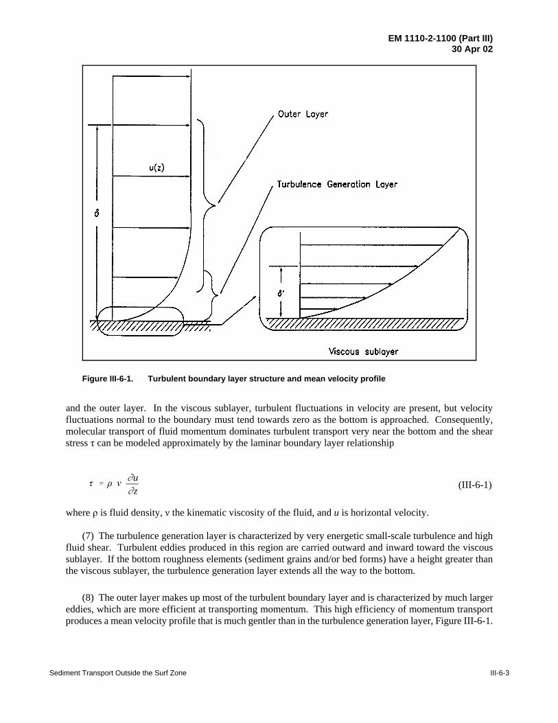
EM 1110-2-1100 (Part III)30 Apr 02
Sediment Transport Outside the Surf Zone III-6-3
Figure III-6-1. Turbulent boundary layer structure and mean velocity profile
τ ' ρ ν MuMz (III-6-1)
and the outer layer. In the viscous sublayer, turbulent fluctuations in velocity are present, but velocityfluctuations normal to the boundary must tend towards zero as the bottom is approached. Consequently,molecular transport of fluid momentum dominates turbulent transport very near the bottom and the shearstress τ can be modeled approximately by the laminar boundary layer relationship
where ρ is fluid density, ν the kinematic viscosity of the fluid, and u is horizontal velocity.
(7) The turbulence generation layer is characterized by very energetic small-scale turbulence and highfluid shear. Turbulent eddies produced in this region are carried outward and inward toward the viscoussublayer. If the bottom roughness elements (sediment grains and/or bed forms) have a height greater thanthe viscous sublayer, the turbulence generation layer extends all the way to the bottom.
(8) The outer layer makes up most of the turbulent boundary layer and is characterized by much largereddies, which are more efficient at transporting momentum. This high efficiency of momentum transportproduces a mean velocity profile that is much gentler than in the turbulence generation layer, Figure III-6-1.

EM 1110-2-1100 (Part III)30 Apr 02
III-6-4 Sediment Transport Outside the Surf Zone
τ ' ρ νTMuMz (III-6-2a)
νT ' κ u(
z (III-6-2b)
uc 'u(c
κln z
zo(III-6-3)
z0 '
ν9u
(
for smooth turbulent flow
kn
30for fully rough turbulent flow
(III-6-4)
(9) Turbulent boundary layer shear flow models can be simply developed by artificially choosing aconstant νT (called the eddy viscosity), which is much larger than its laminar (molecular) value and thatreflects the size of the eddy structure associated with the turbulent flow. This assumption results in a simpleconceptual eddy viscosity model for turbulent shear stress that may be expressed as
with the turbulent eddy viscosity
where κ is known as von Karman's constant and u* = (τb/ρ)1/2 is called the shear velocity, where τb is the shearstress at the bed (z = 0). A complete derivation of this model is given in Madsen (1993).
(10) Experimental determinations have shown relatively little variation of κ, leading to von Karman's“universal” constant assumed to have the value 0.4.
b. Current boundary layer.
(1) Currents on the inner shelf can be considered to flow at a steady velocity compared to the orbitalvelocity of waves. Defining the shear stress due to currents τc, the current velocity profile can be expressedas
where u*c = (τc /ρ)1/2 denotes the current shear velocity. Equation 6-3 is the classic logarithmic velocity profileexpressed in terms of zo, the value of z at which the logarithmic velocity profile predicts a velocity of zero.For a smooth bottom zo = z = 0, but for a rough bottom, the actual location of the boundary is not a singlevalue of z. Hence z = 0 becomes a somewhat ambiguous definition of the “theoretical” location of the bottomwith some portions of the boundary actually located at z > 0 and others at z < 0. Therefore, application ofEquation 6-3 in the immediate vicinity of a solid bottom is purely formal and its prediction of uc = 0 at z =zo is of no physical significance.
(2) From the extensive experiments by Nikuradse (1933), the value of zo is obtained as
in which kn is the equivalent Nikuradse sand grain roughness, so called because Nikuradse in his experimentsused smooth pipes with uniform sand grains glued to the walls, and therefore found it natural to specify thewall roughness as the sand grain diameter. Smooth or fully rough turbulent flow are delineated by Madsen(1993).

EM 1110-2-1100 (Part III)30 Apr 02
Sediment Transport Outside the Surf Zone III-6-5
kn u(
ν$ 3.3 for fully rough turbulent flow
kn u(
ν# 3.3 for fully smooth turbulent flow
(III-6-5)
τc '12
fcρ (uc (zr) )2 (III-6-6)
u(c '
τc
ρ'
fc
2uc(zr) (III-6-7)
(3) For turbulent flows over a plane bed consisting of granular material it is natural to take kn = D =diameter of the grains composing the bed. For flow over a bottom covered by distributed roughness elements(e.g., resembling a rippled bottom), the value kn = 30 z0 is referred to as the equivalent Nikuradse sand grainroughness, with z0 obtained by extrapolation of the logarithmic velocity distribution above the bed, to thevalue z = z0 where uc vanishes.
(4) Figure III-6-2 is a semilogarithmic plot of a current velocity profile obtained over a bottomconsisting of 1.5-cm-high triangular bars at 10-cm spacing (Mathisen 1993). It is noticed that velocitymeasurements over crests and midway between crests (troughs) of the roughness elements deviate from theexpected straight line within the lower 2.5 to 3 cm and further than .10 cm above the bottom. The near-bottom deviations reflect the proximity of the actual bottom roughness elements, which make the velocitya function of location, i.e., the flow is nonuniform immediately above the bottom roughness features. Thenonlogarithmic velocity profile far from the boundary is associated with the flow being that of a developingboundary layer flow in a laboratory flume, i.e., the flow above z . 10 cm is essentially a potential flowunaffected by boundary resistance and wall turbulence.
(5) The well-defined variation of uc versus log z (Figure III-6-2) can be applied to the case 3 cm <z < 10 cm. By extrapolation to uc = 0, one obtains the value z = z0 . 0.7 cm or kn = 30 z0 . 21 cm, since theflow is rough turbulent. This example clearly illustrates that kn, the equivalent Nikuradse sand grainroughness, is a function of bottom roughness configuration and does not necessarily reflect the physical scaleof the roughness protrusions. Thus, the data shown in Figure III-6-2 were obtained for a physical roughnessscale of 1.5 cm, the height of the triangular bars, and result in an equivalent Nikuradse roughness of 21 cm.This large value of kn is, of course, associated with the much larger flow resistance produced by the triangularbars.
(6) It is often convenient to express the bottom shear stress associated with a boundary layer flow interms of a current friction factor fc defined by
(7) The somewhat cumbersome notation used in Equation 6-6 is chosen deliberately to emphasize thefact that the value of the current friction factor is a function of the reference level, z = zr, at which the currentvelocity is specified. From Equation 6-6, the current shear velocity is obtained
and introducing this expression in Equation 6-3, with z = zr and κ = 0.4 leads to an equation for the currentfriction factor

EM 1110-2-1100 (Part III)30 Apr 02
III-6-6 Sediment Transport Outside the Surf Zone
Figure III-6-2. Measured turbulent velocity profile for flow over artificial two-dimensional roughnesselements (Mathisen 1993)
14 fc
. log10zr
z0(III-6-8)
in terms of the reference elevation and the boundary roughness scale.
(8) For rough turbulent flows z0 = kn/30 and Equation 6-8 is an explicit equation for fc in terms of therelative roughness zr/kn. For smooth turbulent flows z0 = ν/(9u*c) and Equation 6-8 leads to an implicitequation for fc (Madsen 1993)

EM 1110-2-1100 (Part III)30 Apr 02
Sediment Transport Outside the Surf Zone III-6-7
EXAMPLE PROBLEM III-6-1
FIND:
The current friction factor fc, the shear velocity u*c, and the bottom shear stress τc, for a current overa flat bed.
GIVEN:
The current is specified by its velocity uc(zr) = 0.35 m/s at zr = 1.00 m. The bottom is flat andconsists of uniform sediment of diameter D = 0.2 mm. The fluid is seawater (ρ . 1,025 kg/m3, ν .1.0×10–6 m2/s).
PROCEDURE:
1) Start with Equation 6-4 assuming rough turbulent flow: z0 = kn/30.
2) Solve Equation 6-8 for fc.
3) Obtain u*c from Equation 6-7.
4) Check rough turbulent flow assumption by evaluating knu*c/ν and using Equation 6-5.
5) If knu*c/ν $ 3.3, flow is rough turbulent. Results (fc and u*c) obtained in steps 2 and 3 constitutethe solution and τc is obtained from Equation 6-6 or from the definition τc = .ρ u 2
(c
6) If knu*c/ν < 3.3, flow is smooth turbulent and the solution is obtained by the following iterativeprocedure (steps 7 and 8).
7) Obtain z0 = ν/(9u*c) using u*c from step 3.
8) With z0 from step 7 return to step 2 to obtain a new fc, and a new u*c from step 3 and reenter(step 7).
9) When consecutive values of u*c agree to two significant digits, iteration is complete. The lastvalues of fc and u*c constitute the solution and τc is obtained from Equation 6-6 or from thedefinition τc = ρ u 2
(c
(Continued)
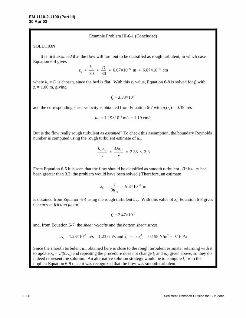
EM 1110-2-1100 (Part III)30 Apr 02
III-6-8 Sediment Transport Outside the Surf Zone
z0 'kn
30'
D30
' 6.67×10&6 m ' 6.67×10&4 cm
knu(c
ν'
Du(c
ν' 2.38 < 3.3
z0 'ν
9u(c
. 9.3×10&6 m
Example Problem III-6-1 (Concluded)
SOLUTION:
It is first assumed that the flow will turn out to be classified as rough turbulent, in which caseEquation 6-4 gives
where kn = D is chosen, since the bed is flat. With this z0 value, Equation 6-8 is solved for fc withzr = 1.00 m, giving
fc = 2.33×10⁻³
and the corresponding shear velocity is obtained from Equation 6-7 with uc(zr) = 0.35 m/s
u*c = 1.19×10⁻² m/s = 1.19 cm/s
But is the flow really rough turbulent as assumed? To check this assumption, the boundary Reynoldsnumber is computed using the rough turbulent estimate of u*c
From Equation 6-5 it is seen that the flow should be classified as smooth turbulent. (If knu*c/ν hadbeen greater than 3.3, the problem would have been solved.) Therefore, an estimate
is obtained from Equation 6-4 using the rough turbulent u*c. With this value of z0, Equation 6-8 givesthe current friction factor
fc = 2.47×10⁻³
and, from Equation 6-7, the shear velocity and the bottom shear stress
u*c = 1.23×10⁻² m/s = 1.23 cm/s and = 0.155 N/m2 . 0.16 Paτc ' ρ u 2(c
Since the smooth turbulent u*c obtained here is close to the rough turbulent estimate, returning with itto update z0 = ν/(9u*c) and repeating the procedure does not change fc and u*c given above, so they doindeed represent the solution. An alternative solution strategy would be to compute fc from theimplicit Equation 6-9 once it was recognized that the flow was smooth turbulent.

EM 1110-2-1100 (Part III)30 Apr 02
Sediment Transport Outside the Surf Zone III-6-9
14 fc
% log101
4 fc
' log10zr uc(zr)
ν% 0.20 (III-6-9)
τw ' ρνtMuw
Mz' ρ κ u
(wm zMuw
Mz(III-6-10)
uw '2π
sin n ubm ln zzo
cos(ω t % n) (III-6-11)
tan n '
π2
lnκu
(wm
zoω&1.15
(III-6-12)
τw ' τωm cos(ω t % n) (III-6-13)
τwm '12
fwρu 2bm (III-6-14)
which shows fc’s dependency on a Reynolds number, , when the flow is classified as smoothzr uc(zr)νturbulent.
c. Wave boundary layers.
(1) Introduction. Wave boundary layers on the inner shelf are inherently unsteady due to the oscillatorynature of near-bottom wave orbital velocity. However, for typical gravity wave periods on the inner shelf,it is assumed that the boundary layer thickness, here denoted by δw, will be sufficiently small so that flow atthe outer edge of the boundary layer may be predicted directly from linear wave theory. An extremecomplication of the unsteady nature of waves arises in the application of the simple turbulent eddy viscositymodel. Specifically, wave turbulent eddy viscosity becomes a time-dependent variable
. However, the effect of a time-varying eddy viscosity is surprisingly small whenu(' (|τb | /ρ)1/2 ' u
((t)
compared with results obtained from a simple time-invariant eddy viscosity model in which is determined from the maximum bottom wave shear stress τwm, during one waveu
(' u
(wm ' ( |τwm | /ρ)1/2
cycle (Trowbridge and Madsen 1984). Therefore, the eddy viscosity model gives a wave shear stress
where uw is the wave orbital velocity (Grant and Madsen 1979, 1986). Using Equation 6-10, applying simplelinear periodic wave theory to the boundary conditions, and simplifying by taking the limiting form of thesolution for the velocity profile gives
in which ubm is the maximum near-bottom wave orbital velocity, ω is 2 π/T, and n, the phase lead of near-bottom wave orbital velocity, is given by
From the near-bottom velocity profile, the bottom shear stress may be obtained from
Expressing the maximum bottom shear stress in terms of a wave friction factor fw defined by Jonsson (1966)
or equivalently

EM 1110-2-1100 (Part III)30 Apr 02
III-6-10 Sediment Transport Outside the Surf Zone
u(wm '
τwm
ρ'
fw
2ubm (III-6-15)
κ 2fw
' lnκ
fw
2ubm
z0ω& 1.15
2
%π2
2 (III-6-16)
Abm 'ubm
ω(III-6-17)
RE 'ubm Abm
ν(III-6-20)
fw '2RE
(III-6-21)
Using Equations 6-10 to 6-15 and simplifying (Madsen 1993) results in an implicit equation for the wavefriction factor
With κ = 0.4 and recognizing that
is the bottom excursion amplitude predicted by linear wave theory, Equation 6-16 may be approximated bythe following implicit wave friction factor relationship (Grant and Madsen 1986)
(III-6-18)14 fw
% log101
4 fw
' log10Abm
kn
& 0.17 % 0.24 4 fw
for rough turbulent flow when kn = 30z0.
For smooth turbulent flow, 30z0 = 3.3ν/u*wm replaces kn in Equation 6-18, which may then be written
(III-6-19)14 4fw
% log101
4 4fw
' log10RE50
& 0.17 % 0.06 4 4fw
in which
is a wave Reynolds number. For completeness, the wave friction factor for a laminar wave boundary layeris given by (Jonsson 1966)
(2) Evaluation of the wave friction factor.
(a) From knowledge of the equivalent roughness kn and wave condition Abm and ubm, three formulas forfw have been presented. The choice of which fw to select is quite simply the largest of the three values. In thiscontext it is mentioned that the wave friction factors predicted for smooth turbulent and laminar flow,

EM 1110-2-1100 (Part III)30 Apr 02
Sediment Transport Outside the Surf Zone III-6-11
1x (n%1)
' log10Abm
kn
& 0.17 & log101
x (n)% 0.24x (n) (III-6-22)
Figure III-6-3. Wave friction factor diagram (a) and bottom friction phaseangle (b)
Equations 6-19 and 6-21, are identical for RE . 3×10⁴, which may be taken as a reasonable value for thetransition from laminar (RE < 3×10⁴) to turbulent flow.
(b) The evaluation of wave friction factors from Equations 6-18 and 6-19 can proceed by iteration. Theiterative procedure is illustrated for Equation 6-18 by writing it in the following form
with the superscript denoting the iteration step and iteration started by choosing x(0) = 0.4.x ' 4 fw
(c) It was assumed, in conjunction with the presentation of Equation 6-11 for the orbital velocity profilewithin the wave boundary layer, that this expression represented an approximation valid only for small valuesof , i.e., for relatively large values of Abm/kn. For this reason and also becausez0ω/(κu
(wm)'(0.12/ fw ) (kn /Abm)the iterative solution of the wave friction factor Equation 6-18 is rather slowly converging for Abm/kn < 100,Figure III-6-3 gives the exact solution for fw and n for Abm/kn < 100.
(d) For smooth turbulent boundary layer flows, Equation 6-19 may be arranged in a fashion similar toEquation 6-22, and the iterative solution proceeds as outlined above with .x ' 4 4fw
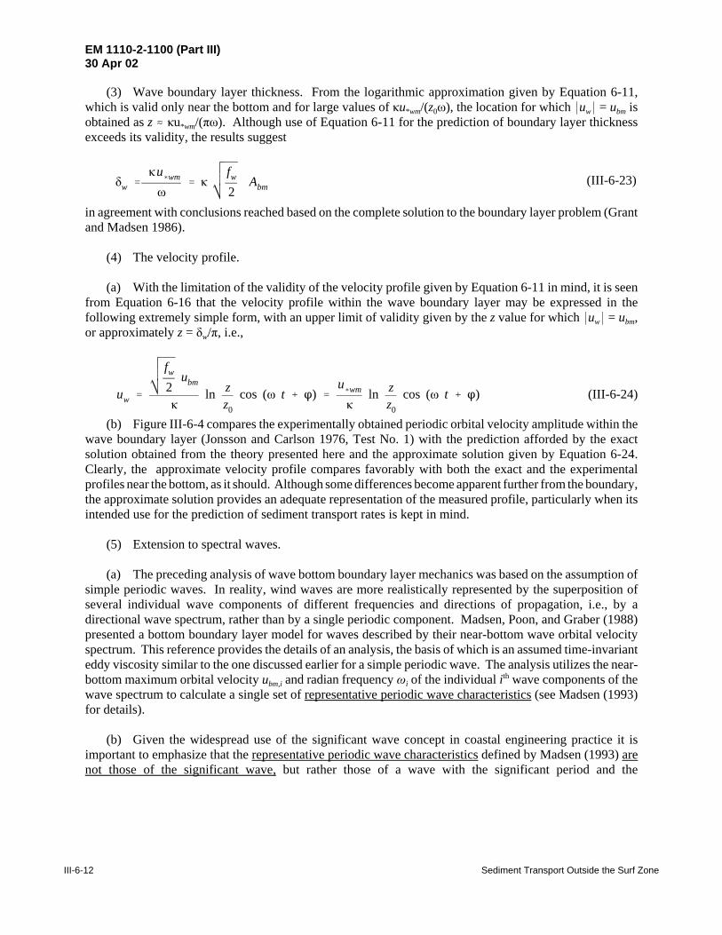
EM 1110-2-1100 (Part III)30 Apr 02
III-6-12 Sediment Transport Outside the Surf Zone
δw 'κu
(wm
ω' κ
fw
2Abm (III-6-23)
(3) Wave boundary layer thickness. From the logarithmic approximation given by Equation 6-11,which is valid only near the bottom and for large values of κu*wm/(z0ω), the location for which *uw* = ubm isobtained as z . κu*wm/(πω). Although use of Equation 6-11 for the prediction of boundary layer thicknessexceeds its validity, the results suggest
in agreement with conclusions reached based on the complete solution to the boundary layer problem (Grantand Madsen 1986).
(4) The velocity profile.
(a) With the limitation of the validity of the velocity profile given by Equation 6-11 in mind, it is seenfrom Equation 6-16 that the velocity profile within the wave boundary layer may be expressed in thefollowing extremely simple form, with an upper limit of validity given by the z value for which *uw* = ubm,or approximately z = δw/π, i.e.,
(III-6-24)uw '
fw
2ubm
κln z
z0
cos (ω t % n) 'u(wm
κln z
z0
cos (ω t % n)
(b) Figure III-6-4 compares the experimentally obtained periodic orbital velocity amplitude within thewave boundary layer (Jonsson and Carlson 1976, Test No. 1) with the prediction afforded by the exactsolution obtained from the theory presented here and the approximate solution given by Equation 6-24.Clearly, the approximate velocity profile compares favorably with both the exact and the experimentalprofiles near the bottom, as it should. Although some differences become apparent further from the boundary,the approximate solution provides an adequate representation of the measured profile, particularly when itsintended use for the prediction of sediment transport rates is kept in mind.
(5) Extension to spectral waves.
(a) The preceding analysis of wave bottom boundary layer mechanics was based on the assumption ofsimple periodic waves. In reality, wind waves are more realistically represented by the superposition ofseveral individual wave components of different frequencies and directions of propagation, i.e., by adirectional wave spectrum, rather than by a single periodic component. Madsen, Poon, and Graber (1988)presented a bottom boundary layer model for waves described by their near-bottom wave orbital velocityspectrum. This reference provides the details of an analysis, the basis of which is an assumed time-invarianteddy viscosity similar to the one discussed earlier for a simple periodic wave. The analysis utilizes the near-bottom maximum orbital velocity ubm,i and radian frequency ωi of the individual ith wave components of thewave spectrum to calculate a single set of representative periodic wave characteristics (see Madsen (1993)for details).
(b) Given the widespread use of the significant wave concept in coastal engineering practice it isimportant to emphasize that the representative periodic wave characteristics defined by Madsen (1993) arenot those of the significant wave, but rather those of a wave with the significant period and the

EM 1110-2-1100 (Part III)30 Apr 02
Sediment Transport Outside the Surf Zone III-6-13
Figure III-6-4. Comparison of present model’s prediction of wave orbital velocity within the waveboundary layer with measurements by Jonsson and Carlson (1976, Test No. 1)
Experimental
z
(em)
Exact Theoretical ~
0 1.2

EM 1110-2-1100 (Part III)30 Apr 02
III-6-14 Sediment Transport Outside the Surf Zone
EXAMPLE PROBLEM III-6-2
FIND:The wave friction factor fw, the maximum shear velocity u*wm, the maximum bottom shear stress τwm,
and the bottom shear stress phase angle n, for a pure wave motion over a flat bed.
GIVEN:The wave is specified by its near-bottom maximum orbital velocity ubm = 0.35 m/s and period
T = 8.0 s. The bottom is flat and consists of uniform sediment of diameter D = 0.1 mm. The fluid isseawater (ρ . 1,025 kg/m3, ν . 1.0×10⁻⁶ m2/s).
PROCEDURE:
1) Compute bottom orbital excursion amplitude from linear wave theory: Abm = (H/2)/sinh(2πh/L) =ubm/ω, using H = Hrms = root-mean-square wave height = , ω = 2π/T with T = significantHs / 2
wave period, and h = water depth. (This step is not needed here, since ubm and T are specified)
2) Assume rough turbulent flow and solve Equation 6-18 using the iterative procedure illustrated byEquation 6-22 for fw.
3) Obtain u*wm from Equation 6-15.
4) Check rough turbulent flow assumption by evaluating knu*wm/ν and using Equation 6-15.
5) If knu*wm/ν $ 3.3, flow is rough turbulent. Results (fw and u*cw) obtained in steps 2 and 3 constitutethe solution. τwm is obtained from Equation 6-14 or 6-15 and n is obtained by solvingEquation 6-12 with z0 = kn/30.
6) If knu*wm/ν < 3.3 flow is smooth turbulent and fw is obtained by solving Equation 6-19 using theiterative procedure illustrated by Equation 6-22 with Abm/kn replaced by andRE/50
x = .4 4fw
7) With fw from step 6, Equation 6-15 gives u*wm and τwm is obtained from Equation 6-14 orEquation 6-15.
8) With u*wm from step 7, the value of z0 = ν/(9u*wm) is obtained from Equation 6-15 for smoothturbulent flow.
9) The phase angle n is calculated from Equation 6-12 using z0 from step 8.
(Sheet 1 of 3)
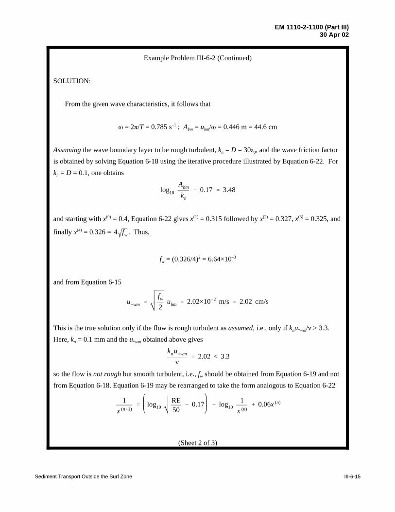
EM 1110-2-1100 (Part III)30 Apr 02
Sediment Transport Outside the Surf Zone III-6-15
log10Abm
kn
& 0.17 ' 3.48
u(wm '
fw
2ubm ' 2.02×10&2 m/s ' 2.02 cm/s
kn u(wm
ν' 2.02 < 3.3
1x (n%1)
' log10RE50
& 0.17 & log101
x (n)% 0.06x (n)
Example Problem III-6-2 (Continued)
SOLUTION:
From the given wave characteristics, it follows that
ω = 2π/T = 0.785 s–1 ; Abm = ubm/ω = 0.446 m = 44.6 cm
Assuming the wave boundary layer to be rough turbulent, kn = D = 30z0, and the wave friction factoris obtained by solving Equation 6-18 using the iterative procedure illustrated by Equation 6-22. Forkn = D = 0.1, one obtains
and starting with x(0) = 0.4, Equation 6-22 gives x(1) = 0.315 followed by x(2) = 0.327, x(3) = 0.325, and
finally x(4) = 0.326 = . Thus,4 fw
fw = (0.326/4)2 = 6.64×10⁻³
and from Equation 6-15
This is the true solution only if the flow is rough turbulent as assumed, i.e., only if knu*wm/ν > 3.3. Here, kn = 0.1 mm and the u*wm obtained above gives
so the flow is not rough but smooth turbulent, i.e., fw should be obtained from Equation 6-19 and notfrom Equation 6-18. Equation 6-19 may be rearranged to take the form analogous to Equation 6-22
(Sheet 2 of 3)

EM 1110-2-1100 (Part III)30 Apr 02
III-6-16 Sediment Transport Outside the Surf Zone
RE 'ubmAbm
ν' 1.56×10⁵
log10RE50
& 0.17 ' 1.58
u(wm '
fw
2ubm ' 2.12×10&2 m/s ' 2.12 cm/s
τwm ' ρ u(wm
2 ' 0.461 N/m 2 ' 0.46 Pa
z0 'ν
9u(wm
' 5.24×10&6 m
Example Problem III-6-2 (Concluded)
with x = and4 4fw
Therefore
and starting iteration with x(0) = 0.0 gives x(1) = 08.29, x(2) = 0.646, x(3) = 0.7,... and finally x(6) =0.686 =
= , or the wave friction factor4 4fw 8 fw
fw = 7.35×10⁻³
which results in the maximum shear velocity
and a maximum bottom shear stress, Equation 6-32,
The phase angle n of the bottom shear stress is obtained from Equation 6-12 with
obtained from Equation 6-4 for smooth turbulent flow
tan n = 0.242 6 n = 13.6E . 14E
(Sheet 3 of 3)

EM 1110-2-1100 (Part III)30 Apr 02
Sediment Transport Outside the Surf Zone III-6-17
Dp '14ρ (fw cosn) u 3
bm (III-6-25)
τm ' *τwm % τ c*
' (τwm % τc *cos φwc*)2 % (τc sin φwc)
2
' τwm 1 % 2τc
τwm
*cos φwc* %τc
τwm
2
(III-6-26)
root-mean-square wave height. Thus, for surface waves specified in terms of their significant height Hs andperiod Ts, the near-bottom representative periodic orbital velocity is obtained from a wave with root meansquare height , and wave period T = Ts . Hrms ' Hs / 2
(6) Dissipation. Time-averaged rate of energy dissipation in the wave bottom boundary layer isobtained from Kajiura (1968) as
for periodic waves and can be extended to spectral waves using the representative periodic wave propertiesas given above (Madsen, Poon, and Graber 1988).
d. Combined wave-current boundary layers.
(1) Introduction.
(a) The simple conceptual model of near-bottom turbulence suggests that the eddy viscosityimmediately above the bottom is a function of time whenever the flow is unsteady. In the context of a purewave motion, it was, however, found that assuming a time-invariant eddy viscosity, based on the maximumshear velocity, resulted in a greatly simplified analysis without sacrificing accuracy appreciably (Trowbridgeand Madsen 1984). In the case of combined wave-current bottom boundary layer flows, the eddy viscosityimmediately above the bottom is therefore scaled by the maximum combined wave-current shear velocity.Since the vertical extent of wave-associated turbulence is limited by the wave bottom boundary layerthickness, the wave contribution to the turbulent mixing must vanish at some level above which only thecurrent shear velocity contributes to turbulent mixing.
(b) For the general case of combined wave-current flows with the current at an angle φwc to the directionof wave propagation, the maximum combined bottom shear stress τm may be obtained from
(c) Since the boundary layer flow for combined waves and currents at an angle is three-dimensional,one should in principle solve for the horizontal velocity vector’s two components. However, when the x-direction is chosen as the wave direction, unsteady flow will exist only in this direction. In this case it canbe shown that all formulas derived for the pure wave case in Part III-6(2)c are valid also for waves in thepresence of a current when u*wm is replaced by u*m obtained from Equation 6-26 with . Foru
(m ' (τm /ρ)1/2

EM 1110-2-1100 (Part III)30 Apr 02
III-6-18 Sediment Transport Outside the Surf Zone
uc 'u(c
κu(c
u(m
ln zz0
(III-6-27)
uc 'u(c
κln z
z0a(III-6-28)
uc 'u(c
κln z
δcw
%u(c
u(m
lnδcw
z0(III-6-29)
u c ' uc(z) {cos φwc, sin φwc} (III-6-30)
example, the velocity profile is given by Equation 6-11 with u*wm replaced by u*m. As mentioned previously,u*wm . u*m, which shows that the wave motion is only weakly influenced by the presence of a current.
(d) The steady flow is entirely in the direction of the current, i.e., at an angle φwc to the wave direction.Invoking the “law of the wall,” the current velocity is (for z < δcw where δcw is defined in Equation 6-38)
and z0 is given by Equation 6-4 with u*m replacing u*.
(e) For z > δcw the solution is
where z0a denotes an arbitrary constant of integration, referred to as the apparent bottom roughness.Matching the two solutions at z = δcw and introducing the expression for z0a in Equation 6-28 gives analternative form of the solution for z > δcw
(f) These expressions clearly reveal the pronounced effect that waves may have on current velocityprofiles. First of all, the velocity gradient inside the wave-current boundary layer is reduced by a factoru*c/u*m relative to its value in absence of waves. This, of course, is a consequence of the increased turbulenceintensity within the wave boundary layer arising from the waves. In the extreme case of u*c/u*m . 0, ucremains nearly zero throughout the wave boundary layer. Thus, currents in the presence of waves experiencean enhanced bottom roughness (i.e., for the same current velocity at a specified level above the bottom the0current shear velocity and shear stress will increase with wave activity).
(g) Figure III-6-5 compares a current velocity profile in the presence of waves predicted by the presentwave-current interaction theory with the measured current profile (Bakker and van Doorn 1978). Twotheoretical predictions are shown, one in which δcw is based on Equation 6-23 with u*wm = u*m and another inwhich δcw was increased by a factor of 1.5. From the comparison, it is concluded that the definition of δcwgiven by Equation 6-23 may be adopted for the wave-current interaction theory presented here. This wave-current interaction theory may be applied to a wave described by its near-bottom orbital velocity spectrumby using the representative periodic wave with the direction of wave propagation chosen as the peak direction(Madsen 1993).
(2) Combined wave-current velocity profile. Having chosen the x-axis as the direction of wave propaga-tion, the wave orbital velocity profile immediately above the bottom is given by Equation 6-11 where thephase angle n defined by Equation 6-12 is evaluated with u*wm = u*m.
The current velocity vector is given by
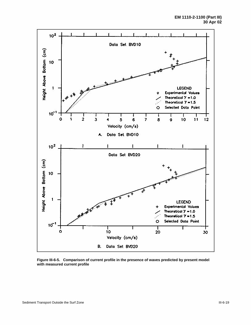
EM 1110-2-1100 (Part III)30 Apr 02
Sediment Transport Outside the Surf Zone III-6-19
Figure III-6-5. Comparison of current profile in the presence of waves predicted by present modelwith measured current profile
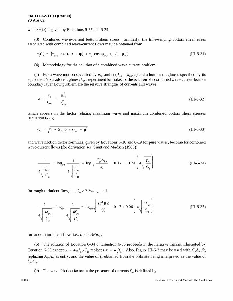
EM 1110-2-1100 (Part III)30 Apr 02
III-6-20 Sediment Transport Outside the Surf Zone
µ 'τc
τwm
'u 2(c
u 2(wm
(III-6-32)
Cµ ' 1 % 2µ cos φwc % µ2 (III-6-33)
where uc(z) is given by Equations 6-27 and 6-29.
(3) Combined wave-current bottom shear stress. Similarly, the time-varying bottom shear stressassociated with combined wave-current flows may be obtained from
(III-6-31)τb(t) ' {τwm cos (ω t % n) % τc cos φwc, τc sin φwc}
(4) Methodology for the solution of a combined wave-current problem.
(a) For a wave motion specified by ubm and ω (Abm = ubm/ω) and a bottom roughness specified by itsequivalent Nikuradse roughness kn, the pertinent formulas for the solution of a combined wave-current bottomboundary layer flow problem are the relative strengths of currents and waves
which appears in the factor relating maximum wave and maximum combined bottom shear stresses(Equation 6-26)
and wave friction factor formulas, given by Equations 6-18 and 6-19 for pure waves, become for combinedwave-current flows (for derivation see Grant and Madsen (1986))
(III-6-34)1
4fcw
Cµ
% log101
4fcw
Cµ
' log10Cµ Abm
kn
& 0.17 % 0.24 4fcw
Cµ
for rough turbulent flow, i.e., kn > 3.3ν/u*m, and
(III-6-35)1
44fcw
Cµ
% log101
44fcw
Cµ
' log10C 2
µ RE50
& 0.17 % 0.06 44fcw
Cµ
for smooth turbulent flow, i.e., kn < 3.3ν/u*m.
(b) The solution of Equation 6-34 or Equation 6-35 proceeds in the iterative manner illustrated byEquation 6-22 except replaces . Also, Figure III-6-3 may be used with CµAbm/knx ' 4 fcw /Cµ x ' 4 fw
replacing Abm/kn as entry, and the value of fw obtained from the ordinate being interpreted as the value offcw/Cµ.
(c) The wave friction factor in the presence of currents fcw is defined by

EM 1110-2-1100 (Part III)30 Apr 02
Sediment Transport Outside the Surf Zone III-6-21
τwm
ρ' u 2
(wm '12
fcw u 2bm (III-6-36)
τm
ρ' u 2
(m ' Cµu 2(wm (III-6-37)
δcw 'κu
(m
ω(III-6-38)
κuc(zr) ' lnzr
δcw
u(c %
lnδcw
z0
u(m
u 2(c
(III-6-39)
and when Equation 6-33 is introduced in Equation 6-26, the maximum combined shear stress reads
(d) Finally, the wave boundary layer thickness is given by the modified form of Equation 6-23, i.e.,
(e) Current specified by τc, i.e., and φwc are known.τc
ρ' u 2
(c
(f) Starting with µ = 0, Cµ = 1, the wave friction factor is obtained from Equation 6-34. The values of u 2(wm
and are obtained from Equations 6-36 and 6-37. Rough turbulent flow is checked by calculating knu*m/ν.u 2(m
If not greater than 3.3, flow is smooth turbulent and the wave friction factor is recalculated from Equation6-35, followed by evaluation of and as before. In most cases, flow is rough turbulent and the checku 2
(m u 2(wm
of rough or smooth turbulent flow is only necessary during the first iteration.
(g) With the pure wave estimate of in hand, one obtains updated values of µ and Cµ fromu 2(wm ' u 2
(m
Equations 6-32 and 6-33. The wave friction factor is obtained from the appropriate relationship, Equa-tion 6-34 or Equation 6-35, by solving for fcw/Cµ followed by multiplication with Cµ. Values of and u 2
(wm u 2(m
are obtained from Equations 6-36 and 6-37. Upon return to Equation 6-32 with the latest value of theu 2(wm
procedure may be repeated until fcw remains essentially unchanged from one iteration to the next. As a reason-able convergence criterion, it is recommended to calculate fcw with no more than three significant figures.
(h) The wave-current interaction problem is now solved and, following evaluation of the wave boundarylayer thickness δcw from Equation 6-38, the current velocity profile may be obtained from Equation 6-27 forz # δcw and from Equation 6-29 for z $ δcw.
(i) Current specified by uc at z = zr (i.e., uc(z = zr)) and φwc are known.
(j) Again µ = 0 and Cµ = 1 are used for the first iteration which proceeds as outlined under step e above.For this case, however, the first iteration is carried through determination of δcw from Equation 6-38. At thispoint, Equation 6-29, assuming zr > δcw, may be regarded as a quadratic equation in the unknown current shearvelocity
with the solution

EM 1110-2-1100 (Part III)30 Apr 02
III-6-22 Sediment Transport Outside the Surf Zone
u(m ' Cµ u
(wm ' u(wm '
fcw
2ubm ' 2.19×10&2 m/s ' 2.19 cm/s
EXAMPLE PROBLEM III-6-3FIND:
The current shear velocity and bottom shear stress, u*c and τc, the maximum wave shear velocity andbottom shear stress, u*wm and τwm, as well as the maximum combined shear velocity and bottom shearstress, u*m and τm, for a combined wave-current flow over a flat bed.
GIVEN:The wave is specified by its near-bottom maximum orbital velocity ubm = 0.35 m/s and period
T = 8 s. The current is specified by its magnitude uc(zr) = 0.35 m/s at zr = 1.00 m and direction φwc = 45Erelative to the direction of wave propagation. The bottom is flat and consists of uniform sediment ofdiameter D = 0.2 mm. The fluid is seawater (ρ = 1,025 kg/m3, ν . 1.0×10⁻⁶ m2/s).
PROCEDURE:
1) Compute wave characteristics as in step 1 of Example Problem III-6-2.
2) Assume rough turbulent flow and solve the wave-current interaction following the iterativeprocedure described in subsection III-6(2)d(4)i.
3) Check if flow is rough turbulent by evaluating knu*m/ν with u*m obtained in step 2.
4) If knu*m/ν $ 3.3, flow is rough turbulent and values of u*c, u*wm, and u*m obtained in step 2constitute the solution. Bottom shear stresses are obtained from the definition of shearvelocities: .τ ' ρu 2
(
5) If knu*m/ν < 3.3 flow is smooth turbulent and the combined wave-current flow is solved as instep 2 except for Equation 6-35 replacing Equation 6-34 when the wave friction factor in thepresence of a current is evaluated.
6) With u*c, u*wm, and u*m from step 5, is used to obtain bottom shear stresses.τ ' ρu 2(
SOLUTION:
For the given wave parameters, ω = 2π/T = 0.785 s–1, Abm = ubm/ω = 0.446 m, and kn = D = 2×10⁻⁴ msince the bottom is flat. Proceeding as outlined in Part III-6(2)d subsection (4)a, starting with µ = 0,Equation 6-33 gives Cµ = 1. Assuming rough turbulent flow, Equation 6-34 reduces to the exact formof the pure wave friction factor Equation 6-18 whose solution is obtained iteratively using Equation 6-22(see Example Problem III-6-2) as
fcw = fw = 7.86×10⁻³
The maximum shear velocity is given by Equation 6-37, i.e.,
(Continued)

EM 1110-2-1100 (Part III)30 Apr 02
Sediment Transport Outside the Surf Zone III-6-23
µ 'u(c
u(wm
2
' 0.45
1x (n%1)
' log10CµAbm
kn
& 0.17 & log101
x (n)% 0.24x (n)
u(wm '
fcw
2ubm ' 2.47×10&2 m/s ' 2.47 cm/s and τwm ' ρu 2
(wm ' 0.624 Pa
u(m ' Cµ u
(wm ' 2.88×10&2 m/s ' 2.88 cm/s and τm ' ρu 2(m ' 0.850 Pa
δcw 'κu
(m
ω' 1.47×10&2 m ' 1.47 cm
Example Problem III-6-3 (Concluded)
since Cµ is currently assumed to be 1. From knu*m/ν = 4.38 it follows that the flow indeed is roughturbulent as assumed. (If knu*m/ν < 3.3, one would have to return and compute fcw fromEquation 6-35.) It therefore follows from Equation 6-38 that
δcw = 1.12×10⁻² m = 1.12 cm
With these values and z0 = kn/30 = D/30 = 6.67×10⁻⁶ m, Equation 6-40 is solved to give a firstestimate of the current shear velocity
u*c = 1.47×10⁻² m/s = 1.47 cm/s
Using the first estimates of u*c = 1.47 cm/s and u*wm = 2.19 cm/s, Equation 6-32 gives
and with φwc = 45E, Equation 6-33 gives Cµ = 1.36.
To solve Equation 6-34 for the wave friction factor in the presence of a current fcw, it is rearranged ina manner identical to Equation 6-22, i.e.,
with . Solving iteratively starting with x(0) = 0.4 gives x(4) = , orx ' 4 fw /Cµ 0.342 ' 4 fw /Cµ
fcw = (x/4)2Cµ = 9.94×10⁻³
The value of the wave shear velocity is now obtained from Equation 6-36
followed by
from Equation 6-37 and
With these values in hand, Equation 6-40 gives a second estimate of the current shear velocity
u*c = 1.63×10⁻² m/s = 1.63 cm/s and τc = = 0.272 Paρu 2(c

EM 1110-2-1100 (Part III)30 Apr 02
III-6-24 Sediment Transport Outside the Surf Zone
Abm
kn
'0.4460.044
. 10
u(wm ' u
(m 'fw
2ubm ' 5.96 cm/s
δcw 'κu
(wm
ω' 3.04 cm
EXAMPLE PROBLEM III-6-4
FIND:The current shear velocity u*c, the maximum wave shear velocity u*wm, the maximum combined shear
velocity u*m, and the wave boundary layer thickness δcw for a combined wave-current turbulent boundarylayer flow.
GIVEN:The wave is specified by its near-bottom maximum orbital velocity ubm = 0.35 m/s and period
T = 8.0 s. The current is specified by its magnitude uc = 0.35 m/s at zr = 1.00 m and direction φwc = 45Erelative to the direction of wave propagation. The equivalent Nikuradse roughness of the bottom iskn = 4.4 cm. The fluid is seawater (ρ = 1,025 kg/m3, ν . 10–6 m2/s).
PROCEDURE:Identical to Example Problem III-6-3. However, the iterative solution of the wave friction factor in
Equation 6-34 is started with an initial value obtained from Figure III-6-3 to speed up convergence.
SOLUTION:For the given wave parameters ω = 2π/T = 0.785 s–1 and Abm = ubm/ω = 0.446 m, the procedure to
follow is identical to that used in Example Problem III-6-3, except that here
is much smaller. Therefore, during the first iteration (with µ = 0 and Cµ = 1) the wave friction factor isobtained from Figure III-6-3
fw = fcw . 0.058instead of solving Equation 6-34. The pure wave approximation therefore gives
and
With these values, the first estimate of the current shear velocity is obtained from Equation 6-40u*c = 2.84 cm/s
(Continued)

EM 1110-2-1100 (Part III)30 Apr 02
Sediment Transport Outside the Surf Zone III-6-25
µ 'u(c
u(wm
2
' 0.23
Example Problem III-6-4 (Concluded)
An updated value of µ is then
and from Equation 6-33
Cµ = 1.17
Recognizing that Equation 6-34 is identical to the pure wave friction factor (Equation 6-18) if
CµAbm/kn replaces Abm/kn and fcw/Cµ replaces fw, the value of fcw/Cµ may be read off Figure III-6-3 when
CµAbm/kn = 11.7 is used as an entry. In this manner
fcw/Cµ . 0.053 6 fcw . 0.062
is obtained. Clearly, the accuracy of the reading obtained from Figure III-6-3 is not impressive, so
the value is regarded only as a rough estimate. From Equation 6-36, Equation 6-37, and
Equation 6-38, it follows that
u*wm = 6.16 cm/s, u*m = 6.67 cm/s, δcw = 3.40 cm
and from Equation 6-40
u*c = 2.94 cm/s
With these values µ = (u*c/u*wm)2 = 0.23, i.e., the iteration is complete.
So the solution is u*c = 2.94 cm/s, τc = = 0.89 Pa, u*wm = 6.16 cm/s, τwm = = 3.89 Pa,ρu 2(c ρu 2
(wm
u*m = 6.67 cm/s, τm = = 4.56 Pa, and δcw = 3.40 cm.ρu 2(m

EM 1110-2-1100 (Part III)30 Apr 02
III-6-26 Sediment Transport Outside the Surf Zone
uc(δcw) 'u(c
κu(c
u(m
lnδcw
z0
' 10.2 cm/s
uc(δcw) 'u(c
κln
δcw
z0a
and solving for z0a gives z0a ' 0.85 cm/s
EXAMPLE PROBLEM III-6-5
FIND:The current velocity uc(δcw) at z = δcw, the apparent roughness z0a, and the phase angle of the wave-
associated bottom shear stress for a combined wave-current bottom boundary layer flow.
GIVEN:Wave, current, and bottom roughness are as specified in Example Problem III-6-4.
PROCEDURE:
1) Solve the wave-current interaction problem following the procedure described for ExampleProblem III-6-4.
2) With u*m, from step 1 δcw is obtained from Equation 6-38.
3) uc (z = δcw) is obtained from Equation 6-27 with z = δcw obtained in step 2 and z0 = kn/30 since flowis rough turbulent. If flow had been smooth turbulent, i.e., knu*m/ν < 3.3, Equation 6-27 is usedwith z0 = ν/(9u*m) as given by Equation 6-5.
4) Equation 6-28 is solved for z0a using u*c from step 1, z = δcw from step 2, and uc = uc(z = δcw) fromstep 3.
5) The phase angle n is obtained from Equation 6-12 with u*wm replaced by u*m from step 1 andz0 = kn/30.
SOLUTION:With u*c = 2.94 cm/s, u*m = 6.67 cm/s, and δcw = 3.40 cm from Example Problem III-6-4,
Equation 6-27 gives (with z0 = kn/30 = 4.4/30 cm)
By matching this with the expression for the current velocity profile outside the boundary layer(Equation 6-28) one obtains
The phase of the wave-associated bottom shear stress is obtained from Equation 6-12 with u*wm replacedby u*m, i.e.,
tan n = 0.79 6 n = 38E

EM 1110-2-1100 (Part III)30 Apr 02
Sediment Transport Outside the Surf Zone III-6-27
Figure III-6-6. Sketch of turbulent flows with logarithmic profile over granular bed
(III-6-40)u(c ' u
(m
lnzr
δcw
lnδcw
z0
&12
%14
% κuc(zr)u(m
lnδcw
z0
lnzr
δcw
2
(k) Having now obtained an estimate of u*c, returning to Equation 6-32 with u*wm known from the firstiteration, the value of µ is updated. With this updated value of µ, the entire procedure is repeated until a newvalue of u*c is obtained. For this iteration, convergence of µ to no more than two significant digits isrecommended.
(l) The theoretical predictions shown in Figure III-6-5 were obtained in this manner using the indicateddata point to specify the current.
III-6-3. Fluid-Sediment Interaction
a. Introduction.
(1) In Part III-6-2, the purely hydrodynamic problem of turbulent bottom boundary layer flows wastreated. There it was found that the fluid-bottom interaction could be represented by a bottom shear stress τb,which, for the general case of combined wave-current flows, is given by Equation 6-31. Since the wavecomponent τwmcos(ωt + n) and the current component τc are both associated with logarithmic velocity profilesimmediately above the bottom, Equations 6-24 and 6-27, respectively, the combined velocity immediatelyabove the bottom is logarithmic.
(2) For a bottom consisting of a granular material, the physical flow condition in the vicinity of theindividual grains is sketched in Figure III-6-6. Recalling that the logarithmic velocity profile in this regionis merely an extrapolation from flow conditions obtained further from the boundary, it is evident that theactual resistance experienced by the flow is not a uniformly distributed force per unit horizontal area, butrather a sum of drag forces on individual grains (roughness elements). Thus, in reality

EM 1110-2-1100 (Part III)30 Apr 02
III-6-28 Sediment Transport Outside the Surf Zone
F'D, grain % τb D 2 (III-6-41)
Wgrain % (ρs & ρ)gD 3 (III-6-42)
ψ 'τb
(ρs & ρ)gD'
τb
(s & 1)ρgD'
u 2(
(s & 1)gD(III-6-43)
τb ' junitarea
F̄D,grain
(3) Not until a level somewhat above the individual roughness elements is it reasonable to assume thateddies, forming around individual grains and ejected into the flow, have merged to produce a turbulent shearflow of the type considered in the conceptual model of turbulent shear stresses presented in Part III-6-2.
(4) In addition to the spatial variation of the actual interaction between a turbulent flow and a granularbottom, it should also be kept in mind that a turbulent flow, even for a steady current, is inherently unsteady.The logarithmic velocity profile represents the time-averaged velocity profile with high-frequency turbulentfluctuations being removed by the averaging process. The drag force on individual grains is therefore notconstant but varies with time due to turbulent fluctuations. The drag forces on individual grains are thereforeaverage values as suggested by the overbar notation.
(5) It is evident from the description above that the complex nature of interaction between a flowingfluid and the individual grains on the fluid-sediment interface defies rigorous mathematical treatment unlessa hydrodynamic model is employed which resolves the flow structure around individual grains includingtemporal variation associated with turbulent fluctuations. Since such a detailed hydrodynamic model is notavailable at present, we are forced to adopt heuristic, physically based conceptual models consistent with thelevel of our flow description to “derive” quantitative relationships for fluid-sediment interaction, and rely onempirical evidence to determine “constants” that are necessary to render the relationships predictive.
b. The Shields parameter.
(1) From the preceding discussion of the nature of near-bottom turbulent flows, it follows that thebottom shear stress may be taken as an expression for the drag force, i.e., the mobilizing force, acting onindividual sediment grains on the bed surface. For a sediment of diameter D there are approximately 1/D2
grains per unit area, so
where the double overbar indicates a temporal, as well as a spatial, average.
(2) For a cohesionless sediment the individual sediment grains rest and stay on the bottom due to theirsubmerged weight and resist horizontal motion due to the presence of neighboring grains. Thus, for acohesionless sediment, the stabilizing force is associated with the submerged weight of the individual grains
where ρs denotes the density of the sediment material (ρs . 2,650 kg/m3 for quartz).
(3) The ratio of mobilizing (drag) and stabilizing (submerged weight) forces is of fundamental physicalsignificance in fluid-sediment interaction for cohesionless sediment. This ratio is known as the Shieldsparameter (Shields 1936)
in which s = ρs/ρ is the density of the sediment relative to that of the fluid.

EM 1110-2-1100 (Part III)30 Apr 02
Sediment Transport Outside the Surf Zone III-6-29
Re('
u(kn
ν'
u(Dν
(III-6-44)
ψcr 'τcr
(s & 1)ρgD'
u 2(cr
(s & 1)gD' f (Re
() (III-6-45)
c. Initiation of motion.
(1) Introduction.
(a) For a turbulent flow over a flat bed consisting of cohesionless sediment of diameter D the equivalentNikuradse sand grain roughness is kn = D. From the discussion of turbulent boundary layer flows it wasfound that the roughness scale experienced by the flow, z0 as given by Equation 6-5, depends on whether theflow is characterized as smooth or rough turbulent. The parameter determining the characteristics of the near-bottom flow and hence the mobilizing force acting on individual sediment grains is the boundary Reynoldsnumber
(b) From simple physical considerations it therefore follows that the conditions of neutral stability ofa sediment grain on the fluid-sediment interface may be expressed as a critical value of the Shields parameter
where f(Re*), which is obtained from models or from experimental data, denotes some function of Re*.Figure III-6-7 shows the traditional Shields diagram given by Equation 6-45 with supporting data obtainedfrom uniform steady flow experiments (Raudkivi 1976). It shows that ψcr . 0.06 is approximately constantfor Re* > 100, i.e., for fully rough turbulent flow, whereas the critical Shields parameter increases steadilyfrom a minimum of 0.035 for values of Re* < 10, i.e., essentially corresponding to smooth turbulent flowconditions.
(c) In establishing the critical condition for initiation of motion, also referred to as threshold or incipientmotion condition (expressed formally by Equation 6-45), it is important to keep in mind the nature of fluid-sediment interaction. For values of ψ > ψcr, mobilizing forces exceed stabilizing forces and sediment motionoccurs. This does not mean that for ψ < ψcr by a small amount, sediment does not move at all. For turbulentflow conditions in the vicinity of ψ . ψcr, the arrival of particularly strong turbulent eddies from theturbulence generation layer may momentarily increase the drag on one or a few sediment grains and, if theresponse time of the individual grains is shorter than the duration of this pulse, a few grains may be dislodged(i.e., a movement of the sediment may occur).The empirical curve on a ψ versus Re* diagram that expressesthe critical condition (i.e., the Shields curve or the Shields criterion) should therefore be interpreted asrepresenting a “gray area” around the curve itself. For flow conditions within this gray area, sedimentmovement may take place but it becomes increasingly sporadic as ψ drops below the curve defining ψcr.
(2) Modified Shields diagram.
(a) In order to predict the flow condition that will cause sediment motion for a given sediment (i.e., sand D known) the traditional Shields curve given by Equation 6-45 or Figure III-6-7 is somewhatcumbersome to use, since the flow characteristic of interest (u*cr) is involved in both parameters. This problemcan be circumvented by recognizing that the Shields curve defines a unique relationship between ψcr and Re*.Thus, from the definition of ψcr (Equation 6-45), one obtains

EM 1110-2-1100 (Part III)30 Apr 02
III-6-30 Sediment Transport Outside the Surf Zone
Figure III-6-7. Shields diagram for initiation of motion in steady turbulent flow(from Raudkivi (1967))
u(cr ' (s & 1) g D ψcr (III-6-46)
S('
D4ν
(s & 1) g D 'Re
(
4 ψcr(III-6-47)
which can be introduced in the definition of Re* to obtain a parameter (Madsen and Grant 1976)
(b) The factor of 4 appears in the definition of S* to render the numerical values of S* comparable withthe Re* values in the traditional Shields diagram. This is done merely for convenience and has no physicalsignificance.
(c) By taking corresponding values of Re* and ψcr from the traditional Shields diagram, one can obtainthe value of the sediment-fluid parameter S*, which in turn can be used to replace Re* in the Shields diagram.In this manner the modified Shields diagram (Madsen and Grant 1976) shown in Figure III-6-8 can beconstructed.
(d) The modified Shields diagram terminates at the lower end of S* at a value of 1 which, for quartzsediments in seawater, corresponds to a sediment diameter of D . 0.1 mm, i.e., a very fine sand. Althoughcohesion may become important for diameters below 0.1 mm, clean silty sediments, i.e., without too muchorganic material and/or clay, can be considered cohesionless and therefore governed by a Shields-typeinitiation of motion criteria. Raudkivi (1976) presents limited experimental data on threshold conditionsobtained for low values of Re* (in the range 0.03 to 1). A best-fit line to the portion of these data obtainedfor grain-shaped sediments gives the following criterion

EM 1110-2-1100 (Part III)30 Apr 02
Sediment Transport Outside the Surf Zone III-6-31
Figure III-6-8. Modified Shields diagram (Madsen and Grant 1976)
ψcr ' 0.1Re&1/3( for Re
(< 1 (III-6-48)
ψcr ' 0.1S &2/7( for S
(< 0.8 (III-6-49)
which upon the modification, i.e., using Equation 6-47, may be written as
(e) For large values of S*, the flow corresponding to initiation of motion is fully rough turbulent,Re* > 100, and the value of ψcr . 0.06 may be used for S* values larger than the range covered inFigure III-6-9.
(3) Modified Shields criterion.
(a) The modified Shields criterion for initiation of motion of a cohesionless sediment shown inFigure III-6-8 was obtained from steady turbulent flow experiments. The fact that this criterion is applicablealso for unsteady turbulent boundary layer flows, as demonstrated by the results presented in Figure III-6-9(Madsen and Grant 1976), is not surprising when the nature of the onset of sediment movement is considered.For flow conditions in the vicinity of ψ . ψcr the sporadic movement of a few grains is, as discussed above,associated with high-frequency turbulent fluctuations in the mobilizing force acting on a grain. Since the near-bottom mean velocity profile is logarithmic for waves as well as for currents, it is physically reasonable toexpect the near-bottom turbulence to be similar, i.e., scaled by the instantaneous value of the bottom shearvelocity. Provided therefore that the response time of the individual sediment grains is short relative to thetime scale of turbulent fluctuations, which are expected to be the same for waves and currents if the shearvelocities are the same, initiation of motion will be affected by unsteadiness only if the wave period is on theorder of the time scale of the turbulent fluctuations. This not being the case, the effects of unsteadiness
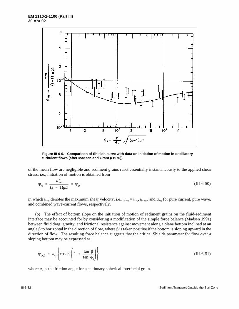
EM 1110-2-1100 (Part III)30 Apr 02
III-6-32 Sediment Transport Outside the Surf Zone
Figure III-6-9. Comparison of Shields curve with data on initiation of motion in oscillatoryturbulent flows (after Madsen and Grant ((1976))
ψm 'u 2(m
(s & 1)gD' ψcr (III-6-50)
ψcr,β ' ψcr cos β 1 %tan βtan φs
(III-6-51)
of the mean flow are negligible and sediment grains react essentially instantaneously to the applied shearstress, i.e., initiation of motion is obtained from
in which u*m denotes the maximum shear velocity, i.e., u*m = u*c, u*wm, and u*m for pure current, pure wave,and combined wave-current flows, respectively.
(b) The effect of bottom slope on the initiation of motion of sediment grains on the fluid-sedimentinterface may be accounted for by considering a modification of the simple force balance (Madsen 1991)between fluid drag, gravity, and frictional resistance against movement along a plane bottom inclined at anangle β to horizontal in the direction of flow, where β is taken positive if the bottom is sloping upward in thedirection of flow. The resulting force balance suggests that the critical Shields parameter for flow over asloping bottom may be expressed as
where φs is the friction angle for a stationary spherical interfacial grain.

EM 1110-2-1100 (Part III)30 Apr 02
Sediment Transport Outside the Surf Zone III-6-33
S('
D4ν
(s & 1)gD ' 2.79
u(cr ' (s & 1)gD ψcr ' 1.27×10&2 m/s ' 1.27 cm/s
EXAMPLE PROBLEM III-6-6
FIND:The critical shear velocity u*cr and critical bottom shear stress τcr for initiation of motion.
GIVEN:Sediment is quartz sand, ρs = 2,650 kg/m3, of diameter D = 0.2 mm. Fluid is seawater (ρ =
1,025 kg-/m3, ν . 1.0×10⁻⁶ m2/s).
PROCEDURE:
1) Compute value of the sediment-fluid parameter S* defined by Equation 6-47.
2) If S* < 0.8 obtain ψcr from Equation 6-49 (be concerned about sediment being cohesive sinceformula is limited to cohesionless sediments).
3) If S* > 300, ψcr . 0.06.
4) If 0.8 < S* < 300 obtain ψcr from Figure III-6-8.
5) Solve Equation 6-45 for u*cr with ψcr obtained in step 2, 3, or 4.
6) Obtain τcr = z from definition of shear velocity.ρ u 2(cr
SOLUTION:The sediment-fluid parameter defined by Equation 6-47 is first computed with s = ρs/ρ = 2.59 and
g = 9.80 m/s2
With this value of S* the critical Shields parameter is obtained from Figure III-6-8
ψcr . 0.052
and using the definition of the Shields parameter given by Equation 6-45
or τcr = ρ(u*cr)2 = 0.165 N/m2 . 0.17 Pa
If S* < 0.8 had been obtained, Equation 6-49 and not Figure III-6-8 should be used to find ψcr.

EM 1110-2-1100 (Part III)30 Apr 02
III-6-34 Sediment Transport Outside the Surf Zone
τb ' τ)b % τ))b (III-6-52)
Figure III-6-10. Conceptualization of pressure drag τbO, skin friction τbN, total shear stress τbN+τbO, forturbulent flow over a rippled bed
d. Bottom roughness and ripple generation. When the flow intensity (expressed in terms of the Shieldsparameter ψ) exceeds the critical condition for initiation of motion ψcr, sediment grains will start to movevirtually instantaneously (Madsen 1991). However, for ψ exceeding ψcr by a modest amount (ψ > (1.1 to1.2)ψcr), the plane bottom will no longer remain plane. It becomes unstable, deforms, and exhibits bed formsand ripples.
(1) The skin friction concept.
(a) The appearance of bed forms on the sediment-fluid interface changes the appearance of the bottomto the flow above. Rather than giving rise to a flow resistance associated with drag forces on individualsediment grains, i.e., a roughness scaled by the sediment diameter, the flow will separate at the crest of thebed forms and flow resistance will primarily be composed of pressure drag forces on bottom bed forms, i.e.,a roughness scaled by the bed form geometry. The appearance of ripples on the bottom changes the physicalbottom roughness by orders of magnitude.
(b) Despite the increased bottom roughness associated with a rippled bed, the drag force acting onindividual sediment grains and not the drag force on the bed forms is responsible for the sediment motioncaused by the flow. In the terminology of bottom shear stresses, it is the average shear stress acting on thesediment grains, the skin friction, that moves sediment and not the total shear stress comprising skin frictionand form drag. The concept of partitioning bottom shear stress into a skin friction and a form drag component,i.e., taking
in which denotes the skin friction component and the form drag component, illustrated in Fig-τ)b τ))bure III-6-10, has received considerable attention in the context of sediment transport mechanics in steadyturbulent flows (Raudkivi 1976).

EM 1110-2-1100 (Part III)30 Apr 02
Sediment Transport Outside the Surf Zone III-6-35
τ)wm '12ρ f )w u 2
bm (III-6-53)
kn ' k )
n ' D (III-6-54)
uc(zr) with zr ' δcw (III-6-55)
ψ)
m 'τ)wm
(s&1)ρgD'
(u )
(wm)2
(s&1)gD(III-6-56)
(c) For a pure wave motion, it is assumed that the skin friction bottom shear stress is obtained quitesimply (Madsen and Grant 1976) by evaluating the bottom shear stress from the given wave condition, ubmand ω, as if the bottom roughness scale were the sediment grain diameter D. Thus, for a wave motion, the skinfriction bottom shear stress is obtained from
where is the wave friction factor obtained from Equation 6-18, Equation 6-19, or Equation 6-21 for af )wroughness
Laboratory data on wave-generated ripples as well as ripple geometry for spectral waves is discussed (Madsen1993) in some detail.
(d) For combined wave-current flows it has been proposed (Glenn and Grant 1987) to evaluate the skinfriction bottom shear stress in a similar manner, i.e., using the wave-current interaction model presented inPart III-b(2)d with a roughness specified by Equation 6-54. However, if a combined wave-current boundarylayer flow is specified by a current velocity outside the wave boundary layer, i.e., uc(zr) with zr > δcw, thedirect use of this information in the formulas given in Part III-6(2)d with kn = = D would lead to ank )
n
ambiguous determination of the skin friction, since this approach presumes the variation of the currentvelocity outside the wave boundary layer to be governed by the grain size roughness, which is true only fora flat bed, i.e., in the absence of form drag.
(e) To overcome this problem, the combined wave-current theory presented in Part III-6(2)d is first usedwith kn = total equivalent Nikuradse sand grain roughness, accounting for the presence of bed forms, topredict the current velocity at the outer edge of the wave boundary layer, i.e.,
is obtained from a model considering total bottom shear stresses.
(f) With the current specified by Equation 6-55, the skin friction shear stress is now computed from thegeneral wave-current interaction theory using the grain size roughness kn = = D. In this mannerk )
n
(Wikramanayake and Madsen 1994a), the ambiguity of the prediction of combined wave-current skin frictionshear stresses is avoided.
(2) Field data on geometry of wave-generated ripples.
(a) When field data on ripple geometry are plotted against the skin friction Shields parameter,

EM 1110-2-1100 (Part III)30 Apr 02
III-6-36 Sediment Transport Outside the Surf Zone
Z 'ψ)
m
S(
(III-6-57)
ηAbm
'
1.8×10&2 Z &0.5 0.0016 < Z < 0.012
7.0×10&4 Z &1.23 0.012 < Z < 0.18
(III-6-58)
ηλ
'
1.5×10&1 Z &0.009 0.0016 < Z < 0.012
1.05×10&2 Z &0.65 0.012 < Z < 0.18
(III-6-59)
kn ' 4η (III-6-60)
they exhibit an extensive scatter. By trial and error it was found (Wikramanayake and Madsen 1994a) thatthe parameter providing the best correlation of field data on ripple geometry was
in which S* is the sediment-fluid parameter defined by Equation 6-47.
(b) The equations for the empirical relationships for ripple geometry in the field are (Madsen 1993).
and
where Abm is defined by Equation 6-17, η is ripple height, λ is ripple length, and the lowest and highest rangeof validity indicate the range covered by the experimental data.
(3) Prediction of ripple geometry under field conditions.
(a) From knowledge of the representative periodic wave (recall that this is defined here as the rms waveand not the significant wave) and sediment characteristics, the skin friction shear stress is obtained fromτ)wm
Equation 6-53.
(b) With known, the value of is obtained from Equation 6-56 and if > ψcr, obtained fromτ)wm ψ)
m 2ψ)
m
the modified Shields curve in Figure III-6-8, sediment motion is assumed to take place and the parameter Zis obtained from Equation 6-57.
With Z known, the empirical relationship given by Equations 6-58 and 6-59 is used to obtain the ripplegeometry. If exceeds a value of 0.35 or if Z > 0.18, the bed is assumed flat corresponding to sheet flowψ)
m
conditions.
e. Moveable bed roughness.
(1) The determination of moveable bed roughness over naturally rippled beds is limited by the lack ofreliable field measurements over a range of wave conditions. The limited amount of available data on wave-generated ripple geometry and the associated rate of energy dissipation in the wave bottom boundary layerabove the rippled bed have been analyzed (Wikramanayake and Madsen 1994a). Their analysis resultssuggest the adoption of the following simple relationship for moveable bed roughness associated with rippledbeds

EM 1110-2-1100 (Part III)30 Apr 02
Sediment Transport Outside the Surf Zone III-6-37
kn ' 15ψ)
m D (III-6-61)
where η is the ripple height. However, the translation of ripple geometry to equivalent roughness, Equa-tion 6-60, is based entirely on laboratory data for periodic waves and is of dubious value for field roughnessdeterminations. Therefore, the following procedure is suggested (Madsen 1993).
(2) For a wave condition specified in terms of the representative periodic wave, the ripple height isobtained from Equation 6-58, and the movable bed roughness kn is obtained from Equation 6-60.
(3) If suggests no sediment motion, < ψcr, the movable bed roughness is taken as kn = = Dψ)
m 2ψ)
m k )
n
unless information on bottom roughness associated with bioturbation of the bottom sediments is available.
(4) If > . 0.35 or if Z > 0.18, the bed is expected to be flat, i.e., corresponding to sheet flowψ)
m
conditions. Recent results from field experiments (Madsen et al. 1993) suggest a value of kn = 15D to beappropriate for sheet flow conditions. Since the conditions from which this result was obtained correspondto values of . 1 and since it is physically reasonable to assume the movable bed roughness for sheet flowψ)
m
conditions depends on the intensity of sediment transport over the flat bed, which in turn is related to themagnitude of , it is tentatively proposed thatψ)
m
be adopted for sheet flow conditions. This expression agrees in form with an expression proposed for steadyflow (Wilson 1989) although the coefficients differ.
III-6-4. Bed-load Transport
a. Introduction.
(1) When flow and sediment characteristics combine to produce a Shields parameter greater than thecritical value, sediment is set in motion. One result of this is the generation of bed forms, discussed inPart III-6-3; another is, of course, the initiation of a non-zero transport of sediment.
(2) For values of the Shields parameter slightly above critical or, more specifically, for low transportrates, the predominant mode of sediment transport takes place as individual grains rolling, sliding, and/orjumping (saltating) along the bed. This mode of sediment transport is referred to as bed load and, since ittakes place in close proximity of the bed, it is dependent on skin friction.
(3) Several empirical bed-load transport formulas have been proposed for steady turbulent boundarylayer flows (Raudkivi 1976). One of these, the Meyer-Peter and Müller formula (Meyer-Peter and Müller1948), enjoys particular popularity in the engineering literature. However, since it was originally developedfrom data obtained for steady flows in rivers and channels of negligible slope, its adoption for unsteady waveor combined wave-current turbulent boundary layer flows over an inclined bed is not straightforward. Aconceptual model for bed-load transport of sediment grains rolling or sliding along an inclined bottom hasbeen proposed (Madsen 1993) as a physical interpretation of the purely empirical Meyer-Peter and Müllerformula. The resulting formulation is time-averaged and solved under the assumptions that: waves dominate

EM 1110-2-1100 (Part III)30 Apr 02
III-6-38 Sediment Transport Outside the Surf Zone
EXAMPLE PROBLEM III-6-7
FIND:
The height η, length λ, and movable bed roughness kn, of wave-generated ripples in the field.
GIVEN:
The representative periodic wave motion is specified as in Example Problem III-6-3. Bottomsediment is quartz, ρs = 2,650 kg/m3, of diameter D = 0.2 mm. Fluid is seawater (ρ = 1,025 kg/m3,ν . 1.0×10⁻⁶ m2/s).
PROCEDURE:
1) Obtain the wave shear velocity assuming grain size roughness = d = median sedimentu )
(wm k )
n
diameter, following the procedure described in Example Problem III-6-2. (Result is denotedhere by prime to signify skin friction shear velocity.)
2) With from step 1 compute from Equation 6-56.u )
(wm ψ)
m
3) Evaluate S* as defined by Equation 6-47.
4) Determine ψcr following procedure of Example Problem III-6-6.
5) If there will be no sediment motion and no ripples, i.e., η = λ = 0. Bottom roughnessψ)
m < ½ψcr
is the sediment grain diameter (kn = = D) unless other information is available, e.g., photosk )
n
showing relict ripples or other roughness features.
6) If > 0.35, sheet flow is assumed. The bed is flat, i.e., η = λ = 0, and the movable bedψ)
m
roughness kn is obtained from Equation 6-61.
7) If ½ψcr < < 0.35, the parameter Z defined by Equation 6-57 is computed.ψ)
m
8) If Z falls within the range indicated for Equations 6-58 and 6-59, these are used to compute η andλ. The movable bed roughness kn is obtained from Equation 6-60.
9) If Z < 0.0016 and D < 0.6 mm, it is recommended that η, λ, and kn be obtained as if Z = 0.0016.
10) If Z > 0.18 and D > 0.08 mm, sheet flow is assumed (i.e., η = λ = 0), and Equation 6-61 is usedto obtain kn.
(Continued)

EM 1110-2-1100 (Part III)30 Apr 02
Sediment Transport Outside the Surf Zone III-6-39
u )
(wm ' f )w/2 ubm ' 2.19×10&2 m/s ' 2.19 cm/s
ψ)
m 'u )
(wm2
(s & 1)gD' 0.154
Z 'ψ)
m
S(
' 0.055
ηAbm
' 7×10&4 Z &1.23 ' 2.47×10&2
η 'η
Abm
Abm ' 1.1 cm
ηλ
' 1.05×10&2 Z &0.65 ' 6.91×10&2 6 λ ' η/(η/λ) ' 15.9 cm . 16 cm
Example Problem III-6-7 (Concluded)
SOLUTION:
In Example Problem III-6-3, the initial solution for the wave friction factor neglected thepresence of a current (µ = 0, Cµ = 1) and gave fw = 7.86×10⁻³. Since the wave motion and the bottomroughness (kn = = D = 0.2 mm) are the same here, the maximum skin friction shear velocity isk )
n
given by
From the definition of the Shields parameter, Equation 6-56, it follows that
The sediment being the same as specified in Example Problem III-6-5 where ψcr = 0.052 wasobtained, it is seen that the sediment will be moving, since . Since < 0.35, flat bedψ)
m > ψcr ψ)
m
(sheet flow) is not predicted and bed forms are therefore expected. The geometry of these bed formsis obtained from the field relationships, Equations 6-58 and 6-59. With the parameter
since S* = 2.79 in Example Problem III-6-6, which is within the range 0.012 < Z < 0.18, onetherefore obtains from Equation 6-58
or, with Abm = 44.6 cm (Example Problem III-6-3)
The ripple steepness is obtained from Equation 6-59
From Equation 6-60, one obtains the movable bed roughness
kn = 4η = 4.4 cm

EM 1110-2-1100 (Part III)30 Apr 02
III-6-40 Sediment Transport Outside the Surf Zone
EXAMPLE PROBLEM III-6-8
FIND:The skin friction shear velocities associated with the current , the wave , and the maximumu )
(c u )
(wm
combined , as well as the phase angle of the wave-associated shear stress nN, for a combined wave-u )
(m
current flow over a movable bed in the field.
GIVEN:
The representative periodic wave is specified by its near-bottom maximum orbital velocity ubm =ubr = 0.35 m/s and period T = 8.0 s. The current is specified by its magnitude uc(zr) = 0.35 m/s atzr = 1.00 m and direction φwc = 45E relative to the direction of wave propagation. The bed consists ofuniform quartz sand, ρs = 2,650 kg/m3, of diameter D = 0.2 mm. The fluid is seawater (ρ = 1,025 kg/m3,ν . 1.0×10⁻⁶ m2/s).
PROCEDURE:
1) Considering only the wave motion, the movable bed roughness kn is obtained following theprocedure given in Example Problem III-6-7.
2) With kn from step 1, the combined wave-current problem is solved following the proceduredescribed in Example Problem III-6-4.
3) From the combined wave-current flow solution obtained in step 2, the current velocity uc(z = δcw)is computed by the procedure of Example Problem III-6-5.
4) With the current specification uc = uc(δcr) at z = δcw from step 3, the wave-current interactionproblem is solved for = D following the procedure described in Example Problem III-6-3.k )
n
5) The skin friction phase angle nN is obtained from Equation 6-12 with .u(wm ' u )
(m
SOLUTION:
The first step to follow in determining the skin friction components for a combined wave-currentboundary layer flow is to determine the movable bed roughness. Since the presence of a current isneglected in performing this step, this was done in Example Problem III-6-7 for the wave and sedimentcharacteristics considered here and resulted in kn = 4.4 cm.
The second step is to determine the current velocity at the edge of the boundary layer, uc(δcw) from thewave-current interaction model using the movable bed roughness obtained in step 1. This was done inExample Problems III-6-4 and III-6-5 where the bottom roughness was specified as kn = 4.4 cm, i.e.,exactly the movable bed roughness determined in step 1 for the given wave and sediment characteristics.
(Continued)

EM 1110-2-1100 (Part III)30 Apr 02
Sediment Transport Outside the Surf Zone III-6-41
u )
(c ' 0.96 cm/s
f )cw ' 8.73×10&3
u )
(wm ' 2.31 cm/s ; u )
(m ' 2.48 cm/s and δ)cw ' 1.26 cm
u )
(c ' 1.01 cm/s
u )
(c ' 1.01 cm/s , u )
(wm ' 2.31 cm/s , u )
(m ' 2.48 cm/s
Example Problem III-6-8 (Concluded)
The third step is to determine the shear velocities and stresses associated with the combined wave-current boundary layer flow over a bottom of roughness kn = = D = sediment diameter with thek )
n
current specified as obtained in step 2. From Example Problem III-6-5, the current specification istherefore
uc(zr) = 10.2 cm/s at zr = δcw = 3.40 cm
at an angle φwc = 45 deg to the direction of wave propagation. With this current specification, kn = = D = 0.2 mm, and wave characteristics ubm = 35 cm/s and ω = 2π/T = 0.785 s–1 (Abm =k )
n
ubm/ω = 44.6 cm) solution of the wave-current interaction problem follows Example Problem III-6-3.
For µ = 0 and Cµ = 1, the first iteration is identical to that in Example Problem III-6-3, resulting in = = 2.19 cm/s and = 1.12 cm. With these values and using the current specificationsu )
(wm u )
(m δ)cw
given above, Equation 6-40 gives
Second iteration is therefore based on µ = = 0.194 and, from Equation 6-33, Cµ = 1.15. u(c)/u )
(wm2
For this value of Cµ solving iteratively for in the manner outlined in Example Problemx ' 4 fcw /Cµ
III-6-3 results in x(3) = 0.349, or
and therefore
with which Equation 6-40 gives
The next value of µ = = 0.191 is virtually identical to the previous value, so no furtheru(w /u )
(wm2
iteration is necessary.
The solution is therefore
and the phase angle of the wave-associated skin friction bottom shear stress is obtained fromEquation 6-12 with and z0 = d/30u
(wm ' u )
(m
tan nN = 0.25 6 φN = 13.8E . 14E

EM 1110-2-1100 (Part III)30 Apr 02
III-6-42 Sediment Transport Outside the Surf Zone
µb 'tanβ
tan φm
<< 1 (III-6-62)
tan φws '23
tan φwc (III-6-65)
µb ' 2µ (III-6-66)
currents ; maximum shear stress is much larger than critical ; and bottomµ ' τ)c /τ)wm <<1 µCR ' τCR /τ)wm <<1slope is relatively small
where β > 0 is bottom slope upward relative to direction of flow and is friction angle (Madsen 1993).φm
Results of this analysis provide the following formulations for the time-averaged bed-load transport .qSB
b. Pure waves on sloping bottom. For a non-zero bottom slope, i.e., µb … 0, but still without anycurrent, the time-averaged net bed-load transport is
(III-6-63)q̄ sB
(s & 1)gDD β
' 8 ψ)
wm
32 *cos θ*
32 6&µb,0> ' 4.5 ψ)
wm
32{&µb,0}
in the direction of the wave propagation, +x, if –µb > 0 and opposite the wave direction if –µb < 0. Sinceµb > 0 if the wave propagates up a slope, βw > 0, and µb < 0 if the wave is directed towards deeper water(βw < 0), this simply states that the net transport is down-slope as expected.
c. Combined wave-current flows. Since the approximate bed-load transport formula is linear in thesmall parameters, the net bed-load transport associated with combined wave-current flows can be evaluatedby time averaging for µb = 0. The resulting net bed-load transport is given by
(III-6-64)q̄ sB
(s & 1)gD D wc
' 6 ψ)
c
32 u )
(wm
u )
(c
32
cos φwc , sin φwc
where denotes the Shields parameter based on the current skin friction shear stress. It should be noted thatψ)
c
the direction of sediment transport is not in the direction of the current but is obtained from
This expression shows that φws, the direction of the net bed-load transport measured counterclockwise fromthe x-axis, deviates from the current direction towards the direction of wave orbital velocities.
d. Combined current and bottom slope effect. It is interesting to note that the superposition of a currentin the direction of wave propagation, i.e., φwc = 0, up a slope may lead to zero net transport. Thus, the sumof transport given by Equations 6-63 and 6-64 is zero if
Although the upslope transport here is associated with an assumed current, it is reasonable to anticipate asimilar upslope effect associated with nonlinear wave effects, i.e., a larger upslope shear stress under the crest

EM 1110-2-1100 (Part III)30 Apr 02
Sediment Transport Outside the Surf Zone III-6-43
q̄ sB ' j fnq̄sB,n (III-6-67)
than the downslope stress under the trough. The balance expressed in Equation 6-66 may therefore be thoughtof as a simulation of an equilibrium profile condition for inner shelf waters.
e. Extension to spectral waves. To compute the bed load for spectral wave conditions, the proceduresoutlined in the foregoing sections are followed using the representative periodic wave characteristics definedin Part III 6-2-b (4).
f. Extension to sediment mixtures.
(1) For a sediment mixture consisting of several distinct size classes of diameter Dn with the volumefraction of the nth size class being fn in the bottom sediments, the total bed-load transport of the sedimentmixture is given by
(2) This extension to sediment mixtures follows directly from the conceptual bed-load transport model(Madsen 1993) when it is assumed that the fraction of excess skin friction shear stress carried by movinggrains of the nth size class is .fn τ
)
b & τcr,n
(3) For each size class, the procedure is therefore exactly as outlined in the preceding section with Dreplaced by Dn, the diameter of the nth size class. The skin friction bottom shear stress is, however, the samefor all size classes and is computed for a single representative grain diameter (D = Dr = D50 = the mediandiameter of the sediment mixture in the bed).
III-6-5. Suspended Load Transport
a. Introduction.
(1) For low transport rates, the predominant mode of transport is sediment grains moving along thebottom, i.e., in the form of bed load. As the flow intensity and, hence, the bed-load transport, is increasedindividual grains moving along the bottom take off from the bottom with increasing frequency, e.g., due toimpact with stationary grains protruding above their neighbors. Thus, as the flow intensity increases, themode of transport changes from one of rolling and sliding along the bottom to one of jumping along thebottom. For this mode of transport, moving grains are in direct contact with immobile bottom grains only fora fraction of the time they spend in transport, and the basic assumptions behind the conceptual transportmodel presented in the preceding section are no longer valid.
(2) Sediment transport associated with individual sediment grains making isolated or a series of jumpsalong the bottom, referred to as saltation, provides a transition from bed-load transport that takes placeimmediately above the bottom to suspended load transport that takes place in the overlying water column.From this distinction between the bed-load and suspended load transport modes, it follows that suspendedload is governed by the turbulence associated with the total bottom shear stress, i.e., the shear stress predictedfrom the movable bed roughness estimate obtained from Part III-6-3, whereas the bed load is governed bythe skin friction shear stress.

EM 1110-2-1100 (Part III)30 Apr 02
III-6-44 Sediment Transport Outside the Surf Zone
EXAMPLE PROBLEM III-6-9FIND:
The bed-load transport rate for a combined wave-current flow over a sloping bottom.
GIVEN:
The wave is specified by its maximum near-bottom orbital velocity ubm = 0.35 m/s, period T = 8.0 s,and angle of incidence α = 45 deg. The current is at an angle of φwc = 45 deg to the wave direction andhas a magnitude of uc(zr) = 0.35 m/s at zr = 1.00 m. The bottom has a uniform slope of β = 1 deg andconsists of uniform quartz sand ρs = 2,650 kg/m3, with diameter D = 0.2 mm. The fluid is seawater (ρ =1,025 kg/m3, ν . 1.0×10⁻⁶ m2/s).
PROCEDURE:
1) The skin friction shear velocities and stresses are computed using the procedure of ExampleProblem III-6-8.
2) The skin friction Shields parameters, and , are obtained from Equation 6-43 with u* = ψ)
c ψ)
wm u )
(c
and , respectively, as obtained in step 1.u )
(wm
3) The time-averaged combined wave-current bed-load transport vector is obtained from Equa-
tion 6-64 using and from step 1 and from step 2.u )
(c u )
(wm ψ)
c
4) The bottom slope parameter µb is calculated from Equation 6-62, where β is bottom slope in thedirection of wave propagation (positive if wave is traveling towards shallower waters) andφm = 30 deg.
5) The time-averaged bottom slope bed-load transport vector is obtained from Equation 6-63 with ψ)
wm
from step 2.
6) The total time-averaged bed-load transport vector is obtained by vector addition of the wave-current and slope bed-load transport vectors obtained in step 3 and step 5, respectively. (Thex component denotes the transport in the direction of wave propagation, the y component istransport 90 deg counterclockwise to the direction of wave propagation.)
(Continued)

EM 1110-2-1100 (Part III)30 Apr 02
Sediment Transport Outside the Surf Zone III-6-45
ψ)
c ' 0.033 and ψ)
wm ' 0.17
q̄ sB
(s & 1)gDD wc
' 0.082 32
cos φwc , sin φwc
q̄ sB wc' {9.7,6.5}×10&3 cm 3/(cm s)
q̄ sB
(s & 1)gDD β
' 0.32{&µb,0}
q̄ sB β' {&7.5,0}×10&4 cm 3/(cm s)
q̄ sB ' q̄ sB wc% q̄ sB β
. {9.0,6.5}×10&3 cm 3/(cm s)
Example Problem III-6-9 (Concluded)
SOLUTION:To calculate bed-load transport, one needs to use skin friction shear stresses. The problem
specification is here identical to that of Example Problem III-6-8, so the skin friction problem was
solved there, i.e., = 1.01 cm/s and = 2.31 cm/s. The corresponding skin friction Shieldsu )
(c u )
(wm
parameters are obtained from Equation 6-56 with s = ρs/ρ = 2.59 and D = 0.2 mm
With these values, the bed-load transport associated with the combined wave-current flow isobtained in nondimensional form from Equation 6-64
or in dimensional form with φwc = 45 deg
To obtain the contribution due to bottom slope, the slope βw in the direction of wave propagation isneeded. Since the bottom slope is β = 1 deg and the angle of incidence is α = 45 deg, the bottomslope in the direction of wave propagation is tan βw = tan β cos α = 0.012. Equation 6-62 thereforegives, with φm = 30 deg, µb = tan βw/tan φm = 0.021. Bed-load transport due to bottom slope isobtained from Equation 6-63 in nondimensional form
or in dimensional form
The total bed-load transport rate is obtained as the sum of the wave-current and bottom slopecontributions, i.e.,
with the x component being in the direction of wave propagation and the y component being at90 deg counterclockwise from the wave direction.

EM 1110-2-1100 (Part III)30 Apr 02
III-6-46 Sediment Transport Outside the Surf Zone
vs ' vt ' ku(
z (III-6-68)
(ρs & ρ) g π6
D 3 '12ρ CD
π4
D 2 w 2f (III-6-69)
wf
(s & 1) g D'
43 CD
(III-6-70)
wf
(s & 1) g D' 1.82 for S
(> 300 (III-6-71)
wf
(s & 1) g D'
29
S(
for S(
< 0.8 (III-6-72)
(3) Distribution of suspended sediment in the water column is governed by the fall velocity of thesediment wf, the sediment diffusion coefficient vs, and the volume concentration of sediment in suspension c.Assuming the sediment-fluid mixture behaves as a clear fluid, a close analogy can be drawn between theturbulent diffusion of momentum and sediment diffusion such that
For combined wave-current bottom boundary layer flows, the concentration of suspended sediments c maybe resolved into its mean and time-varying wave-associated cw components.c̄
b. Sediment fall velocity.
(1) In order to solve the equations governing the distribution of suspended sediment concentration inthe vertical, it is necessary to obtain the value of the sediment fall velocity wf.
(2) Assuming a spherical sediment grain, the force balance of submerged weight and fluid drag on agrain falling through an otherwise quiescent fluid gives
or
(3) The drag coefficient CD is a function of the Reynolds number ReD = D wf /v, which is a function ofS*, the sediment-fluid parameter defined by Equation 6-47.
(4) From the empirical relationship of CD versus ReD (Schlichting 1960), CD is obtained for a specifiedvalue of Red. With this value of CD the nondimensional fall velocity is obtained from Equation 6-70, and thisvalue is used with the specified value of ReD to obtain the corresponding value of S*. In this manner (Madsenand Grant 1976), the graph of nondimensional fall velocity as a function of the sediment fluid parameter,shown in Figure III-6-11, is obtained.
(5) Extending the graph to values of S* above the upper limit of Figure III-6-11 is accomplished byusing
(6) For values of S* below unity, i.e., for quartz grains of d < 0.1 mm in seawater, the fall velocity isobtained from Stokes Law, which in the present notation may be written

EM 1110-2-1100 (Part III)30 Apr 02
Sediment Transport Outside the Surf Zone III-6-47
Figure III-6-11. Nondimensional fall velocity for spherical particles versus the sediment fluid parameter(Madsen and Grant 1976)
(7) Although Figure III-6-11 is obtained for sediment assumed to be spherical, it yields reasonablyaccurate fall velocities for natural cohesionless granular sediments (Dietrich 1982).
c. Reference concentration for suspended sediments.
(1) Introduction.
(a) With the fall velocity determined, all parameters in the equation governing the suspended sedimentconcentration distribution are in principle known. To solve the equation it is, however, necessary to specifyboundary conditions. One boundary condition is simply that no sediment is transported through the watersurface or that the suspended sediment concentration vanishes at large distances above the bottom, if thewater depth is sufficiently large. Another is the boundary condition that expresses the amount of sedimentavailable for entrainment immediately above the bottom. Whereas the former is universally agreed upon thelatter boundary condition is the subject of considerable controversy. It is beyond the scope of this presentationto get into the subtleties of this controversy, so the most commonly accepted form of the bottom boundarycondition for suspended sediment concentration, the specification of a reference concentration, is adoptedhere.
(b) The reference concentration is given as (Madsen 1993)

EM 1110-2-1100 (Part III)30 Apr 02
III-6-48 Sediment Transport Outside the Surf Zone
cR ' γCb*τ)b(t)*τcr,β
& 1 (III-6-73)
S('
D4ν
(s & 1) g D ' 2.79
wf
(s & 1) g D. 0.40
γ '
2×10&3 for rippled bed
2×10&4 for flat bed
(III-6-74)
EXAMPLE PROBLEM III-6-10
FIND:Find the sediment fall velocity
GIVEN:Sediment is quartz sand, ρs = 2,650 kg/m3, of diameter D = 0.2 mm.Fluid is seawater (ρ = 1,025 kg/m3, υ . 1.0×10⁻⁶ m2/s).
PROCEDURE:1) The sediment-fluid parameter S*, defined by Equation 6-47, is calculated.
2) If S* > 300, the sediment fall velocity wf is obtained from Equation 6-71.
3) If S* < 0.8, the sediment fall velocity wf is obtained from Equation 6-72.
4) If 0.8 < S* < 300, wf is obtained from Figure III-6-11 using S* from step 1 as entry.
SOLUTION:The sediment-fluid parameter is calculated from
with s = ρs/ρ = 2.59.
Figure III-6-11 then gives the nondimensional fall velocity
and thereforewf = 2.23 cm/s
in which γ is the so-called resuspension parameter and Cb is the volume concentration of sediment in the bed,generally taken as 0.65 (Smith and McLean 1977) for a bed consisting of cohesionless sediment.
(c) It is emphasized that the resuspension parameter γ in Equation 6-73 is intimately related to thechoice of reference elevation zr, which explains at least part of the considerable variability of γ valuesreported in the literature. Similarly, γ values reported in the literature can be used only in conjunction withtheir particular zr values. This being said, the numerical values

EM 1110-2-1100 (Part III)30 Apr 02
Sediment Transport Outside the Surf Zone III-6-49
c̄R ' γ Cb2π
u )
(wm
u(cr
2
& 1
c̄R ' 1.44×10&3 (cm 3/cm 3)
EXAMPLE PROBLEM III-6-11
FIND:The reference concentration for suspended sediment computations for combined wave-current
boundary layer flows.
GIVEN:Wave, current, sediment, and bottom slope specifications are identical to those of Example
Problem III-6-9.
PROCEDURE:
1) Skin friction shear velocities and stresses are computed following the procedure of ExampleProblem III-6-8.
2) The time-averaged (mean) reference concentration is obtained from Equation 6-75 withc̄R
Cb = 0.65, , and τcr as obtained in step 1, and the appropriate choice of γ fromτ)wm
Equation 6-74.
3) The periodic (wave) reference concentration cRw is obtained from Equation 6-76 using γ and Cb
as in step 2 and shear velocities obtained in step 1. The bottom slope in the direction of wavepropagation βw is positive if the wave is traveling up-slope, and φm = 30 deg.
SOLUTION:The reference concentration for suspended load computations depends on skin friction shear
velocities, obtained in Example Problem III-6-8 for the same problem specification as here, and may beseparated into a mean and a periodic component.
The mean reference concentration is given by Equation 6-75, which may alternatively be written
where = 2.31 cm/s (Example Problem III-6-8) and u*cr = 1.27 cm/s (Example Problem III-6-6). Theu )
(wm
resuspension parameter is given by Equation 6-74. Since the bed is rippled for these problem specifica-tions, cf. Example Problem III-6-7, γ = 2×10⁻³ is chosen here. With Cb = 0.65 the mean referenceconcentration is
(Continued)

EM 1110-2-1100 (Part III)30 Apr 02
III-6-50 Sediment Transport Outside the Surf Zone
cRwm ' γ Cb4π
u )
(c
u(cr
2
cos φwc &u )
(wm
u(cr
2tan βw
tan φm
c̄R ' γ Cb2π
τ)wm
τcr
& 1 (III-6-75)
Example Problem III-6-11 (Concluded)
The periodic reference concentration is given by Equation 6-76. The maximum value may be written
which is evaluated using = 1.01 cm/s (Example Problem III-6-8), φwc = 45 deg, andu )
(c
tan βw/tan φm = µb = 0.021 (Example Problem III-6-9) to give the wave-associated maximumreference concentration
cRwm = 0.65×10⁻³ (cm3/cm3)
with a temporal variation cos (ωt + nN) with nN = 14 deg (Example Problem III-6-8). Both mean andperiodic reference concentrations are specified at
zR = 7D = 0.14 cm
obtained for and from a model closely resembling the present model, with reference elevation zR = 7D, areadopted here (Wikramanayake and Madsen 1994b). It should, however, be emphasized that there isconsiderable uncertainty associated with the adoption of these γ values, or any other values for that matter.
(d) To evaluate the general expression for the reference concentration given by Equation 6-73 forcombined wave-current flows, the assumption of wave dominance is introduced in the context of evaluationof bed-load transport as previously done in Part III-6-4. Subject to the limitations stated there, the referenceconcentration is valid for dominant wave conditions ( ) exceeding critical conditions ( )τ)c < < τ)wm τcr << τ)wm
over a gently sloping bottom (tanβw « tanφm).
(2) Mean reference concentration. From the general expression for the reference concentration (Madsen1993), the time-invariant, mean reference concentration is obtained as
and is applied at z = zr = 7D.
(3) Wave reference concentration. The periodic component of the reference concentration (Madsen1993), the wave reference concentration, is given by

EM 1110-2-1100 (Part III)30 Apr 02
Sediment Transport Outside the Surf Zone III-6-51
θ ' ωt % n) (III-6-77)
νs '
κu(m z z < δcw
κu(c z z > δcw
(III-6-78)
δcw 'κu
(m
ω(III-6-79)
c̄ ' c̄Rzzr
&wf
κ u(m for z < δcw
(III-6-80)
c̄ ' c̄Rδcw
zr
&wf
κu(m z
δcw
&wf
κu(c for z > δcw
(III-6-81)
(III-6-76)cRw ' γ Cb4π
τ)cτcr
cos φwc &τ)wm
τcr
tan βw
tan φm
cos θ ' cRwm cos θ
at z = zr = 7D. In this expression it is recalled that the wave phase is given by
where nN is the phase angle given by Equation 6-14 for skin friction conditions, i.e., with .u(wm ' u )
(m
d. Concentration distribution of suspended sediment. For a combined wave-current flow, the eddyviscosity or eddy diffusivity is given by
with
and the shear velocities being those determined from the wave-current interaction model described inPart III-6-2-c using the equivalent Nikruradse roughness corresponding to the movable bed roughnessobtained by the procedures outlined in Part III-6(3)e.
(1) Mean concentration distribution. Using the equation governing the distribution of mean concentra-tion (Madsen 1993), and introducing the eddy diffusivity from Equation 6-78 yields
and
where c̄R is given by Equation 6-75, and the mean concentrations are matched at z = δcw.
(2) Wave-associated concentration distribution. The wave-generated suspended sediment concentrationcan be approximated as (Madsen 1993)
(III-6-82)cw . cRwm cos(ω t % n)) & cRwm2π
sin ns ln zzr
cos (ω t % n) % ns)

EM 1110-2-1100 (Part III)30 Apr 02
III-6-52 Sediment Transport Outside the Surf Zone
tan ns '
π2
lnκu
(m
zrω& 1.15
(III-6-83)
q̄sS,T ' mh
zr
u c c̄ dz % mh
zr
uw cw dz (III-6-84)
q̄sS ' mh
zr
uc c̄ dz (III-6-85)
q̄sSw ' mh
zr
uw cw dz (III-6-86)
where
This is a highly simplified solution for the wave-associated suspended sediment concentration within thewave boundary layer, i.e., for z < δcw. For a more accurate representation of the wave-associated concentrationprofile, reference is made to Wikramanayake and Madsen (1994b).
e. Suspended load transport. The suspended load transport is obtained from the product of the velocityvector, and the concentration of suspended sediment followed by integration over depth is denoted by h.Time averaging the instantaneous transport rate produces a net transport rate, which is the quantity of interest.Indicating time-averaging by an overbar, the total net suspended load transport rate is obtained from
This equation identifies the contribution to the total net suspended load transport as one associated entirelywith mean suspended load transport
which takes place in the direction of the current ,i.e., at an angle φwc to the direction of wave propagation, andmean wave-associated suspended load transport
which is in the direction of wave propagation when positive.
(1) Mean suspended load transport. The mean suspended load transport, given by Equation 6-85, mustbe considered for two specific conditions.
(a) When zr > z0, the current velocity profile is valid for z $ zr and the mean suspended load transportis obtained from
(III-6-87)q̄sS 'u(c
κc̄R
δcw
zr
&wf
κu(m δcw (I1 % I2) for zr > z0

EM 1110-2-1100 (Part III)30 Apr 02
Sediment Transport Outside the Surf Zone III-6-53
uc 'u(c
κu(c
u(m
lnδcw
z0
lnδcw
zr
ln zzr
for z < δcw (III-6-90)
q̄sS 'u(c
κc̄R
δcw
zr
&wf
κu(m δcw (I3 % I2) for zr < z0 (III-6-91)
where
(III-6-88)I1 'κu
(c
κu(m & wf
lnδcw
z0
&κu
(m
κu(m & wf
&zr
δcw
κu(m & wf
κu(m ln
zr
z0
&κu
(m
κu(m & wf
represents the contribution from inside the wave boundary layer; and
(III-6-89)I2 'κu
(c
κu(c & wf
hδcw
κu(c & wf
κu(c ln h
z0a
&κu
(c
κu(c & wf
& lnδcw
z0a
&κu
(c
κu(c & wf
expresses the transport above the wave boundary layer.
(b) When zr < z0, the current velocity profile is not defined for zr < z < z0. To remedy this physicallyunrealistic situation, the current velocity profile given by Equation 6-27 is modified to read
for the purpose of evaluating the transport within the wave boundary layer. The modification retains thematching condition with the outer solution at z = δcw and extends the velocity profile down to z = zR.
(c) Introducing Equation 6-90 in the integration leads to
where
(III-6-92)I3 '
lnδcw
z0
lnδcw
zr
κu(c
κu(m & wf
lnδcw
zr
&κu
(m
κu(m & wf
1 &zr
δcw
κu(m & wf
κu(m
and I2 is given by Equation 6-89.
(2) Mean wave-associated suspended load transport. The mean wave-associated suspended loadtransport is obtained from Equation 6-86. Since uw and cw, given by Equations 6-11 and 6-82, respectively,are approximations valid only for z < δcw/π, the integration is extended only to this upper limit. Similar to thecomputation of the mean suspended load transport, it is necessary here to distinguish between the two casesof z0 < zr and zr < z0. If zr > δcw/π, wave-associated transport is considered negligibly small.

EM 1110-2-1100 (Part III)30 Apr 02
III-6-54 Sediment Transport Outside the Surf Zone
EXAMPLE PROBLEM III-6-12
FIND:The mean suspended load transport rate for a combined wave-current boundary layer flow.
GIVEN:Wave, current, sediment, and bottom slope as given in Example Problem III-6-9. Water depth
h = 5.0 m.
PROCEDURE:1) Movable bed roughness kn is determined as described in Example Problem III-6-7.
2) Total shear velocities u*c, u*wm, and u*m, and wave boundary layer thickness δcw are obtained bysolving the wave-current interaction following the procedure of Example Problem III-6-4 withkn from step 1.
3) Apparent bottom roughness z0a and shear stress phase angle n are obtained as described inExample Problem III-6-5.
4) Skin friction shear velocities , , and , and phase angle nN are obtained as in Exampleu )
(c u )
(wm u )
(m
Problem III-6-8.
5) Example Problem III-6-10 is followed to obtain the fall velocity wf.
6) Mean reference concentration is obtained as in Example Problem III-6-11.c̄R
7) If zr = 7D > z0 = kn/30, the mean suspended sediment transport is obtained from Equa-q̄sS
tions 6-87 through 6-89.
8) If zr = 7D < z0 = kn/30, the mean suspended sediment transport is obtained from Equa-q̄sS
tions 6-91, III-6-92, and 6-89.
9) The mean suspended sediment transport obtained in step 7 or step 8 is in the direction of thecurrent, which in turn is at an angle of φwc to the direction of wave propagation. In a coordinatesystem with x in the direction of wave propagation, the mean suspended sediment transportvector is .q̄ sS ' q̄sS 6cosφwc, sinφwc >
(Continued)

EM 1110-2-1100 (Part III)30 Apr 02
Sediment Transport Outside the Surf Zone III-6-55
u(c
κc̄R
δcw
zr
&wf
κu(m δcw ' 2.5×10&3 cm 3/(cm s)
I3 '3.123.19
× 2.68{3.19 & 6.08[1 & 0.59]} ' 1.83
I2 ' &1.12[0.012(6.38 % 1.12) & (1.39 % 1.12)] ' 2.71
q̄sS ' 2.5×10&3(I3 % I2) ' 1.1×10&2 cm 3/(cm s)
Example Problem III-6-12 (Concluded)
SOLUTION:
Since quantities needed for the computation of suspended load transport have been obtained inprevious example problems, these are summarized here.
Reference concentration (Example Problem III-6-11): = 1.44×10⁻³ at zr = 0.14c̄R
Fall velocity (Example Problem III-6-10): wf ' 2.23 cm/s
Shear velocities and wave boundary layer thickness based on total movable bed roughness(Example Problem III-6-4): u
(c ' 2.94 cm/s, u(m ' 6.67 cm/s, and δcw ' 3.40 cm
The movable bed roughness and the apparent bottom roughness(Example Problems III-6-7 and III-6-5): z0 ' kn/30 ' 0.15 cm and z0a ' 0.85 cm
From the input values summarized above it is seen that zr = 0.14 cm . z0 = 0.15 cm. One couldtherefore choose either Equation 6-87 or Equation 6-91 to obtain the mean suspended load transport.Since zr < z0, Equation 6-91 is chosen here.
The leading term in Equation 6-91 is computed first
The integral I3 is evaluated from Equation 6-92
and I2 is obtained from Equation 6-89
The mean suspended load transport is therefore obtained from Equation 6-91 as
and is in the direction of the current, i.e., at an angle φwc = 45 deg to the direction of wavepropagation.

EM 1110-2-1100 (Part III)30 Apr 02
III-6-56 Sediment Transport Outside the Surf Zone
I4 ' lnδcw
πz0
& 1 &πzr
δcw
lnzr
z0
& 1 (III-6-94)
I6 ' lnδcw
πzr
& 1 %πzr
δcw(III-6-97)
I7 ' lnδcw
πzr
2
& 2 lnδcw
πzr
% 2 1 &πzr
δcw(III-6-98)
(a) For z0 < zr < δcw/π, Equations 6-11 and 6-82 may be introduced directly into Equation 6-86 to give
(III-6-93)q̄sSw '
1π2
sinn ubm cRwm δcw
× cos (n & n))I4 &2π
sin ns cos (n & n) & ns)I5 for z0 < zr
in which
and
(III-6-95)I5 ' lnzr
z0
lnδcw
πzr
& 1 %πzr
δcw
% lnδcw
πzr
2
& 2 lnδcw
πzr
% 2 1 &πzr
δcw
(b) For zr < z0 the same modification of the logarithmic velocity profile introduced in the context ofmean suspended load transport yields, for zr < z0
(III-6-96)q̄sSw '
1π2
sin n ubm cRwm δcw
lnδcw
πz0
lnδcw
πzr
× cos (n & n))I6 &2π
sin nscos (n & n) & ns)I7
where
and
EM 1110-2-1100 (Part III)30 Apr 02
Sediment Transport Outside the Surf Zone III-6-57
EXAMPLE PROBLEM III-6-13
FIND:
The mean wave-associated suspended load transport rate for a combined wave-current boundary
layer flow.
GIVEN:
Same problem specifications as in Example Problem III-6-12.
PROCEDURE:
1) First steps are identical to steps 1 and 2 in Example Problem III-6-12.
2) If zr = 7D > δcw/π, wave-associated suspended sediment transport is negligibly small.
3) If zr = 7D < δcw/π, steps 3 through 5 of Example Problem III-6-12 are followed.
4) The wave-associated reference concentration cRw is obtained as in Example Problem III-6-11.
5) The sediment suspension phase angle ns is obtained from Equation 6-83 with zr = 7D.
6) If zr = 7D > z0 = kn/30, the mean wave-associated suspended sediment transport is obtainedq̄sSw
from Equations 6-93 through 6-95.
7) If zr = 7D < z0 = kn/30, the mean wave-associated suspended sediment transport is obtainedq̄sSw
from Equations 6-96 through 6-98.
8) The suspended sediment transport obtained in step 6 or step 7 is in the direction of wave
propagation, i.e., uu with x in the direction of wave propagation.q̄ sSw ' q̄sSw61, 0>
(Continued)

EM 1110-2-1100 (Part III)30 Apr 02
III-6-58 Sediment Transport Outside the Surf Zone
1π2
sin n ubm cRwm δcw
lnδcw
πz0
lnδcw
πzr
' 5.0×10&3 cm 3/(cm s)
Example Problem III-6-13 (Concluded)
SOLUTION:In addition to the quantities given in Example Problem III-6-12, the computation of the mean
wave-associated suspended load transport requires knowledge of phase angles
n = 38E and nN = 14E
obtained from Example Problems III-6-5 and 8. The sediment suspension phase angle ns is obtainedfrom Equation 6-83 with zr = 7D = 0.14 cm
tan ns = 0.77 6 ns = 37.6E . 38E
and the maximum wave-associated reference concentration (Example Problem III-6-11) is
cRwm = 0.65×10⁻³
Since zr = 0.14 cm < z0 = 0.15 cm, the wave-associated mean transport is obtained fromEquation 6-96.
The leading term of this equation becomes
and the integral I6 is obtained from Equation 6-97
I6 = 2.05 - 1 + 0.13 = 1.18and I7 is given by Equation 6-98
I7 = 4.18 - 4.09 + 2(1 - 0.13) = 1.83Introducing these quantities in Equation 6-96, the mean wave-associated suspended load transport isobtained as
q̄sSw ' 5.0×10&3 1.18 cos (38E & 14E) & 1.83 2π
sin 38E cos (38E& 14E & 38E) ' 1.9×10&3 cm 3/(cm s)
The direction of this transport is in the direction of wave propagation.

EM 1110-2-1100 (Part III)30 Apr 02
Sediment Transport Outside the Surf Zone III-6-59
(3) Computation of total suspended load transport for combined wave-current flows.
(a) With the wave and current components of the skin friction bottom shear stress including the phaseangle nN obtained following the procedures given in Part III-6-3-c, the mean c̄R and wave-associated cRwmreference concentrations are obtained from Equations 6-75 and 6-76, respectively, and the phase angle forthe wave-associated concentration ns is obtained from Equation 6-83.
(b) From the hydrodynamic wave-current interaction model corresponding to movable bed roughness,u*c, u*wm, u*m, and n are known and wf is obtained from Part III-6-5-a. Thus, with δcw given by Equation 6-79,all quantities necessary to evaluate Equations 6-87 and 6-93, for z0 < zr = 7D, or Equations 6-91 and 6-96,for zr = 7D < z0, are available.
f. Extensions of methodology for the computation of suspended load.
(1) Extension to spectral waves. For a wave motion described by its near-bottom orbital velocityspectrum, the representative periodic wave characteristics discussed in Part III-6-2-b (4) are used. Once againit is emphasized that this representative wave corresponds to the use of the rms wave height and not thesignificant wave height.
(2) Extension to sediment mixtures. For a sediment mixture, the suspended load transport may becalculated as described above for a single grain size of diameter D.
(a) The skin friction and movable bed roughness kn are computed using the median grain sizeτ)b(t)D = D50.
(b) For each grain size class of diameter Dn, the reference concentration is obtained from the formulasgiven in Part III-6(5)c with τcr, the critical shear stress, replaced by τcr,n, the critical shear stress for the nth sizeclass, and Cb, the sediment concentration in the bed, being replaced by fnCb where fn, is the volume fractionin the bed of sediment of diameter Dn. This reference concentration is assumed to be specified at z = zr = 7D50for all size classes.
(c) For each size class, the suspended load transport is now computed as detailed in Part III-6(5)e usingthe fall velocity wf,n appropriate for the nth size class.
(d) When suspended load transport has been obtained for each size class, the total suspended loadtransport for the sediment mixture is obtained by adding the contribution of individual size classes.
III-6-6. Summary of Computational Procedures
a. Problem specification. A properly posed problem requires the following specifications:
(1) The waves are specified by near-bottom orbital velocity ubm, radian frequency ω (Abm = ubm/ω), andtheir angle of incidence α (*α* < π/2) if waves are traveling towards shallower water). For spectral waves, arepresentative periodic wave is defined in Part III-6(2)c(5). If the significant wave characteristics Hs and Ts
are given, the equivalent periodic wave has a height and period T = Ts.Hrms'hs / 2(2) The current is specified by a reference current uc(zr) at z = zr above the bottom and its direction φwc
measured counterclockwise from the direction of wave propagation; or by the average bottom shear stressτc and its direction φwc.

EM 1110-2-1100 (Part III)30 Apr 02
III-6-60 Sediment Transport Outside the Surf Zone
(3) The fluid is specified by its density, ρ . 1,025 km/m3 for seawater, and kinematic viscosity, ν .10–6 m2/s for seawater.
(4) The sediment is specified by its diameter D and density ρs (s = ρs/ρ). The sediment must be character-ized as cohesionless.
(5) The bottom slope is specified normal to depth contours by tanβ (β > 0). The slope in direction ofwave propagation is then tanβw = tanβcosα > 0 if bottom is sloping upwards in wave direction (*α* < π/2).
b. Model parameters.
(1) A number of model parameters and constants have been introduced and must be specified to proceedtowards a solution
κ = von Karman’s constant = 0.4
φs = static friction angle of sediment = 50E
φm = moving friction angle of sediment = 30E
Cb = volume concentration of sediment in the bed = 0.65
γ = resuspension parameter = 2×10⁻³ for rippled beds, 2×10⁻⁴ for flat beds (sheet flow)
(2) Figure III-6-12 specifies coordinate, angle, and bottom slope definitions used in this chapter.
c. Computational procedures. The following steps should be followed to obtain the total sedimenttransport rate at a point:
(1) Movable bottom roughness is determined from the wave and sediment characteristics. The maximumwave skin friction shear stress is obtained following the procedures described in Part III-6(2)c using kn = τ)wm k )
n
= D. Sediment motion is checked using the modified Shields diagram, Part III-6(3)c. If sediment is notmoving, kn = D is the movable bed roughness. If sediment is found to move, the movable bed roughness kn
is obtained following the procedures outlined in Part III-6(3)e using .τ)wm ' τ)m
(2) With the movable bed roughness kn known, the wave-current interaction model (Part III-6(2)d) isused to obtain total bottom shear stresses, shear velocities, and phase angles so that wave orbital and currentvelocity profiles may be evaluated.
(3) Using the current at the edge of the wave boundary layer obtained from the movable bed roughnessmodel as the current specification, the wave-current interaction model (Part III-6(2)d) is used with = Dk )
n
to obtain the combined wave-current skin friction shear stress .τ)b(t)
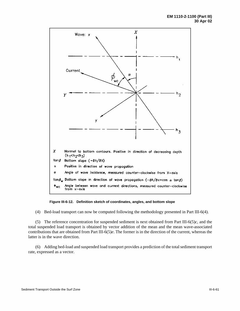
EM 1110-2-1100 (Part III)30 Apr 02
Sediment Transport Outside the Surf Zone III-6-61
Figure III-6-12. Definition sketch of coordinates, angles, and bottom slope
(4) Bed-load transport can now be computed following the methodology presented in Part III-6(4).
(5) The reference concentration for suspended sediment is next obtained from Part III-6(5)c, and thetotal suspended load transport is obtained by vector addition of the mean and the mean wave-associatedcontributions that are obtained from Part III-6(5)e. The former is in the direction of the current, whereas thelatter is in the wave direction.
(6) Adding bed-load and suspended load transport provides a prediction of the total sediment transportrate, expressed as a vector.
EM 1110-2-1100 (Part III)30 Apr 02
III-6-62 Sediment Transport Outside the Surf Zone
*q̄ sT* ' q̄ 2sT,x % q̄ 2
sT,y ' 2.4×10&2 cm 3/(cm s)
EXAMPLE PROBLEM III-6-14
FIND:The total sediment transport vector for a combined wave-current boundary layer flow.
GIVEN:All problem specifications are identical to those given in Example Problems III-6-9, 12, and 13.
PROCEDURE:1) Bed-load sediment transport vector is computed following Example Problem III-6-9.
2) Mean suspended sediment transport vector is obtained following the procedure of ExampleProblem III-6-12.
3) Mean wave-associated suspended sediment transport vector is obtained from ExampleProblem III-6-13.
4) Total sediment transport vector is obtained as the vector sum of steps 1, 2, and 3.
SOLUTION:With x being in the direction of wave propagation and y perpendicular to x, the total sediment
transport in the x direction is obtained from Example Problems III-6-9, 12, and 13.
x-component of bed load = 9.0×10⁻³ cm3/(cm s)x-component of mean suspended load = 1.1×10⁻² cos φwc = 7.8×10⁻³ cm3/(cm s)x-component of mean wave-associated transport = 1.9×10⁻³ cm3/(cm s)Total transport in wave direction = = 1.9×10⁻² cm3/(cm s)q̄sT,x
y-component of bed load = 6.5×10⁻³ cm3/(cm s)y-component of mean suspended load = 1.1×10⁻² sin φwc = 7.8×10⁻³ cm3/(cm s)y-component of mean wave-associated transport = 0 cm3/(cm s)Total transport perpendicular to wave direction = = 1.4×10⁻² cm3/(cm s)q̄sT,y
Thus, the magnitude of the total sediment transport vector is
directed at an angle φwT . 37E to the wave direction.

EM 1110-2-1100 (Part III)30 Apr 02
Sediment Transport Outside the Surf Zone III-6-63
III-6-7. References
Bakker and van Doorn 1978Bakker, W. T., and Van Doorn, T. 1978. "Near-Bottom Velocities in Waves with a Current," ProceedingsSixteenth International Coastal Engineering Conference, American Society of Civil Engineers, Vol 2,pp 1394–1413.
Bijker 1967Bijker, E.W. 1967. “Some Considerations about Scales for Coastal Models with Movable Bed,” TechnicalReport, Delft Hydraulics Lab, The Netherlands.
Davies, Soulsby, and King 1988Davies, A. G., Soulsby, R. L., and King, H. L. 1988. “A Numerical Model of the Combined Wave andCurrent Bottom Boundary Layer,” Journal of Geophysical Research, Vol 93, No. C1, pp 491 - 508.
Dietrich 1982Dietrich, W. E. 1982. “Settling Velocity of Natural Particles,” Water Resources Research, Vol 18, No. 6,pp 1615–1626.
Dyer and Soulsby 1988Dyer, K. R., and Soulsby, R.L. 1988. “Sand Transport on the Continental Shelf,” Annual Review of FluidMechanics, Vol 20, pp 295-324.
Fredsoe 1984Fredsoe, J. 1984. “Sediment Transport in Current and Waves,” Series Paper 35, Institute of Hydrodynamicsand Hydrologic Engineering, Technical University of Denmark, Lyngby.
Glenn and Grant 1987Glenn, S. M., and Grant, W. D. 1987. “A Suspended Sediment Correction for Combined Wave and CurrentFlows,” Journal of Geophysical Research, Vol 92, No. C8, pp 8244–8264.
Grant and Madsen 1979Grant, W. D., and Madsen, O. S. 1979. “Combined Wave and Current Interaction with a Rough Bottom,”Journal of Geophysical Research, Vol 85, No. C4, pp 1797–1808.
Grant and Madsen 1982Grant, W. D., and Madsen, O. S. 1982. “Movable Bed Roughness in Unsteady Oscillatory Flow,” Journalof Geophysical Research, Vol 87, No. C1, pp 469–481.
Grant and Madsen 1986Grant, W. D., and Madsen, O. S. 1986. “The Continental Shelf Bottom Boundary Layer,” M. Van Dyke, ed.,Annual Review of Fluid Mechanics, Vol 18, pp 265–305.
Heathershaw 1981Heathershaw, A.D. 1981. “Comparisons of Measured and Predicted Sediment Transport Rates in TidalCurrents,” Marine Geology, Vol 42, pp 75-104.
Jonsson 1966Jonsson, I. G. 1966. “Wave Boundary Layers and Friction Factors,” Proceedings of the Tenth InternationalCoastal Engineering Conference, American Society of Civil Engineers, Vol 1, pp 127–148.

EM 1110-2-1100 (Part III)30 Apr 02
III-6-64 Sediment Transport Outside the Surf Zone
Jonsson and Carlson 1976Jonsson, I. G., and Carlsen, N. A. 1976. “Experimental and Theoretical Investigation in an OscillatoryTurbulent Boundary Layer,” Journal of Hydraulic Research, Vol 14, No. 1, pp 45–60.
Kajiura 1968Kajiura, K. 1968. “A Model of the Bottom Boundary Layer in Water Waves,” Bulletin of the EarthquakeResearch Institute, Disaster Prevention Research Institute, Tokyo University, Vol 46, pp 75–123.
Madsen 1991Madsen, O. S. 1991. “Mechanics of Cohesionless Sediment Transport in Coastal Waters,” Proceedings,Coastal Sediments ’91, American Society of Civil Engineers, Vol 1, pp 15–27.
Madsen 1992Madsen, O. S. 1992. “Spectral Wave-Current Bottom Boundary Layer Flows,” Abstracts, Twenty-ThirdInternational Coastal Engineering Conference, American Society of Civil Engineers, pp 197–198.
Madsen 1993Madsen, O.S. 1993. “Sediment Transport Outside the Surf Zone,” unpublished Technical Report, U.S. ArmyEngineer Waterways Experiment Station, Vicksburg, MS.
Madsen and Grant 1976Madsen, O. S., and Grant, W. D. 1976. “Quantitative Description of Sediment Transport by Waves,”Proceedings, Fifteenth International Coastal Engineering Conference, American Society of Civil Engineers,Vol 2, pp 1093–1112.
Madsen and Wikramanayake 1991Madsen, O. S., and Wikramanayake, P. N. 1991. “Simple Models for Turbulent Wave-Current BottomBoundary Layer Flow,” Contract Report DRP-91-1, U.S. Army Engineer Waterways Experiment Station,Vicksburg, MS.
Madsen et al., in preparationMadsen, O. S., Wright, L. D., Boon, J. D., and Chisholm, T. A. “Wind Stress, Bottom Roughness andSediment Suspension on the Inner Shelf during an Extreme Storm Event,” in preparation, Continental ShelfResearch.
Madsen, Poon, and Graber 1988Madsen, O. S., Poon, Y.-K., and Graber, H. C. 1988. “Spectral Wave Attenuation by Bottom Friction:Theory,” Proceedings, Twenty-First International Coastal Engineering Conference, American Society ofCivil Engineers, Vol 1, pp 492–504.
Mathisen 1993Mathisen, P.P. 1993. “Bottom Roughness for Wave and Current Boundary Layer Flows over a Rippled bed,”Ph.D. diss., Department of Civil and Environmental Engineering, Massachusetts Institute of Technology,Cambridge, MA.
Meyer-Peter and Müller 1948Meyer-Peter, E., and Müller, R. 1948. “Formulas for Bed-Load Transport,” Report on Second Meeting ofInternational Association for Hydraulic Research, pp 39–64.

EM 1110-2-1100 (Part III)30 Apr 02
Sediment Transport Outside the Surf Zone III-6-65
Nikuradse 1933Nikuradse, J. 1933. “Strömungsgesetze in rauhen Rohren,” VDI Forschungsheft No. 361 (English translationNACA Technical Memorandum No. 1292).
Raudkivi 1976Raudkivi, A. J. 1976. Loose Boundary Hydraulics (2nd ed.), Pergamon Press, Oxford, England.
Schlichting 1960Schlichting, H. 1960. Boundary Layer Theory (fourth ed.), McGraw-Hill, New York.
Shields 1936Shields, A. 1936. “Application of Similarity Principles and Turbulent Research to Bed-Load Movement,”(translation of original in German by W. P. Ott and J. C. van Uchelen, California Institute of Technology),Mitteilungen der Preussischen Versuchsanstalt für Wasserbau und Schiffbau.
Smith 1977Smith, J. D. 1977. “Modeling of Sediment Transport on Continental Shelves,” The Sea, E. D. Goldberg, ed.,Wiley Interscience, New York, pp 539–577.
Smith and McLean 1977Smith, J. D., and McLean, S. R. 1977. “Spatially Averaged Flow Over a Wavy Surface,” Journal ofGeophysical Research, Vol 82, No. 12, pp 1735–1745.
Trowbridge and Madsen 1984Trowbridge, J. H., and Madsen, O. S. 1984. “Turbulent Wave Boundary Layers,” Journal of GeophysicalResearch, Vol 89, No. C5, pp 7989–8007.
White, Milli, and Crabbe 1975White, W.R., Milli, H., and Crabbe, H.O. 1975. “Sediment Transport Theories: A Review,” Proceedings,Institute of Civil Engineering, Vol 59, pp 265-292.
Wikramanayake and Madsen 1994aWikramanayake, P. N., and Madsen, O. S. 1994a. “Calculation of Movable Bed Friction Factors,” ContractReport DRP-94-5, U.S. Army Engineer Waterways Experiment Station, Vicksburg, MS.
Wikramanayake and Madsen 1994bWikramanayake, P. N., and Madsen, O. S. 1994b. “Calculation of Suspended Sediment Transport byCombined Wave-Current Flows,” Contract Report DRP-94-7, U.S. Army Engineer Waterways ExperimentStation, Vicksburg, MS.
Wilson 1989Wilson, K. C. 1989. “Friction of Wave Induced Sheet Flow,” Coastal Engineering, Vol 12, pp 371–379.

EM 1110-2-1100 (Part III)30 Apr 02
III-6-66 Sediment Transport Outside the Surf Zone
III-6-8. Definition of Symbols
β Bottom slope [deg]
βw Bottom slope in the direction of wave propagation [deg]
γ Resuspension parameter [dimensionless]
δcw Boundary layer thickness for a combined wave-current turbulent boundary layer[length]
δw Boundary layer thickness [length]
η Ripple height [length]
κ von Karman’s constant (= 0.4)
λ Ripple length [length]
µ Ratio of Shear stress due to currents (τc) to Maximum bottom shear stress (τwm)
µb Bottom slope parameter
ν Kinematic viscosity [length2/time]
νs Sediment diffusion coefficient
νT Turbulent eddy viscosity [length2/time]
ρ Mass density of water (salt water = 1,025 kg/m3 or 2.0 slugs/ft3; fresh water =1,000kg/m3 or 1.94 slugs/ft3) [force-time2/length4]
ρs Mass density of sediment grains [force-time2/length4]
τb Bottom shear stress [force/length2]
τc Shear stress due to currents [force/length2]
τcr Critical bottom shear stress for initiation of motion [force/length2]
τm Maximum combined bottom shear stress [force/length2]
τw Bottom shear stress [force/length2]
τwm Maximum bottom shear stress [force/length2]
τNb Bottom skin friction shear stress [force/length2]
τNwm Skin friction bottom shear stress for wave motion [force/length2]
τNNb Bottom drag shear stress [force/length2]
n Phase lead of near-bottom wave orbital velocity (bottom shear stress phase angle)[deg]
nm Friction angle [deg]
ns Friction angle for a stationary interfacial sediment grain [deg]

EM 1110-2-1100 (Part III)30 Apr 02
Sediment Transport Outside the Surf Zone III-6-67
Ψ Shields parameter (Equation III-6-43) [dimensionless]
Ψcr Critical Shields parameter (Equation III-6-45) [dimensionless]
Ψcr,β Critical Shields parameter for flow over a sloping bottom (Equation III-6-51)[dimensionless]
ΨNC Shields parameter based on the current skin friction shear stress [dimensionless]
ΨNm Skin friction Shields parameter [dimensionless]
ω Wave angular or radian frequency (= 2π/T) [time-1]
Abm Bottom excursion amplitude predicted by linear wave theory [length]
c Volume concentration of sediment in suspension [length3/length3]
c& Mean volume concentration of sediment in suspension [length3/length3]
c&R Mean reference concentration [length3/length3]
Cµ Factor relating maximum wave and maximum combined bottom shear stresses(equation III-6-33)
Cb Volume concentration of sediment in the bed
cR Reference concentration [length3/length3]
cRwm Wave-associated maximum reference concentration [length3/length3]
cw Wave-associated volume concentration of sediment in suspension [length3/length3]
D Sediment grain diameter [length - generally millimeters]
Dp Time-averaged rate of energy dissipation in the wave bottom boundary layer(Equation III-6-25)
fc Current friction factor [dimensionless]
fcw Wave friction factor in the presence of currents [dimensionless]
fw Wave friction factor [dimensionless]
fNw Wave friction factor [dimensionless]
g Gravitational acceleration (32.17 ft/sec2, 9.807m/sec2) [length/time2]
h Water depth [length]
Hrms Root-mean-square wave height [length]
Hs Significant wave height [length]
kn Equivalent Nikuradse sand grain roughness [length]
kn Movable bed roughness [length]
q Sediment transport rate [length3/time]

EM 1110-2-1100 (Part III)30 Apr 02
III-6-68 Sediment Transport Outside the Surf Zone
q&sB Total bed-load transport of a sediment mixture [length3/length-time]
RE Wave Reynolds number [dimensionless]
Re* Boundary Reynolds number [dimensionless]
S* Sediment-fluid parameter (Equation III-6-47) [dimensionless]
T Significant wave period [time]
Ts Significant wave period [time]
u Horizontal particle velocity [length/time]
u* Shear velocity [length/time]
u*c Current shear velocity [length/time]
u*cr Critical shear velocity [length/time]
u*m Maximum combined shear velocity [length/time]
u*wm Maximum wave shear velocity [length/time]
ubm Maximum near-bottom wave orbital velocity [length/time]
uw Wave orbital velocity [length/time]
wf Sediment fall velocity [length/time]
Wgrain Submerged weight of individual sediment grains
z Elevation from bottom [length]
Z Parameter providing a correlation of field data on ripple geometry [dimensionless]
z0a Arbitrary constant of integration (apparent bottom roughness)

EM 1110-2-1100 (Part III)30 Apr 02
Sediment Transport Outside the Surf Zone III-6-69
III-6-9. Acknowledgments
Authors of Chapter III-6, “Sediment Transport Outside the Surf Zone:”
Ole S. Madsen Ph.D., Dept. of Civil and Environmental Engineering, Massachusetts Institute ofTechnology, Cambridge, Massachusetts.
William Wood, Ph.D. (Deceased).
Reviewers:
Scott M. Glenn, Ph.D., Institute of Marine and Coastal Sciences, Rutgers University, New Brunswick,New Jersey.
James R. Houston, Ph.D., Engineer Research and Development Center, Vicksburg, Mississippi.Stephen McLean, Ph.D., Department of Mechanical and Environmental Engineering, University of
California, Santa Barbara, Santa Barbara, California.Todd L. Walton, Ph.D., Coastal and Hydraulics Laboratory, Engineer Research and Development Center
(ERDC), Vicksburg, Mississippi.