Coastal and Hydraulics Laboratory - DTIC · The Coastal Inlets Research Program (CIRP) of the U.S....
132
ERDC/CHL TR-08-13 Coastal Inlets Research Program CMS-Wave: A Nearshore Spectral Wave Processes Model for Coastal Inlets and Navigation Projects Lihwa Lin, Zeki Demirbilek, Hajime Mase, Jinhai Zheng, and Fumihiko Yamada August 2008 Coastal and Hydraulics Laboratory Approved for public release; distribution is unlimited.
Transcript of Coastal and Hydraulics Laboratory - DTIC · The Coastal Inlets Research Program (CIRP) of the U.S....
ERD
C/CH
L TR
-08-
13
Coastal Inlets Research Program
CMS-Wave: A Nearshore Spectral Wave Processes Model for Coastal Inlets and Navigation Projects
Lihwa Lin, Zeki Demirbilek, Hajime Mase, Jinhai Zheng, and Fumihiko Yamada
August 2008
Coas
tal a
nd H
ydra
ulic
s La
bora
tory
Approved for public release; distribution is unlimited.
Coastal Inlets Research Program ERDC/CHL TR-08-13 August 2008
CMS-Wave: A Nearshore Spectral Wave Processes Model for Coastal Inlets and Navigation Projects
Lihwa Lin and Zeki Demirbilek U.S. Army Engineer Research and Development Center Coastal and Hydraulics Laboratory 3909 Halls Ferry Road Vicksburg, MS 39180-6199, USA
Hajime Mase Disaster Prevention Research Institute Kyoto University Gokasho, Uji, Kyoto, 611-0011, JAPAN Jinhai Zheng Hohai University Research Institute of Coastal and Ocean Engineering 1 Xikang Road, Nanjing, 210098, China Fumihiko Yamada Kumamato University Graduate School of Science and Technology 2-39-1, Kurokami, Kumamoto, 860-8555, JAPAN Final report Approved for public release; distribution is unlimited
Prepared for U.S. Army Corps of Engineers Washington, DC 20314-1000
Monitored by Coastal and Hydraulics Laboratory U.S. Army Engineer Research and Development Center 3909 Halls Ferry Road, Vicksburg, MS 39180-6199
ERDC/CHL TR-08-13 ii
Abstract: The U.S. Army Corps of Engineers (USACE) plans, designs, constructs, and maintains jetties, breakwaters, training structures, and other types of coastal structures in support of Federal navigation projects. By means of these structures, it is common to constrain currents that can scour navigation channels, stabilize the location of channels and entrances, and provide wave protection to vessels transiting through inlets and navigation channels. Numerical wave predictions are frequently sought to guide management decisions for designing or maintaining structures and inlet channels.
The Coastal Inlets Research Program (CIRP) of the U.S. Army Engineer Research and Development Center (ERDC), Coastal and Hydraulics Laboratory (CHL), in collaboration with two universities in Japan, has developed a spectral wave transformation numerical model to address needs of USACE navigation projects. The model is called CMS-Wave and is part of Coastal Modeling System (CMS) developed in the CIRP. The CMS is a suite of coupled models operated in the Surface-water Modeling System (SMS), which is an interactive and comprehensive graphical user interface environment for preparing model input, running models, and viewing and analyzing results. CMS-Wave is designed for accurate and reliable representation of wave processes affecting operation and maintenance of coastal inlet structures in navigation projects, as well as in risk and reliability assessment of shipping in inlets and harbors. Important wave processes at coastal inlets are diffraction, refraction, reflection, wave breaking, dissipation mechanisms, and the wave-current interaction. The effect of locally generated wind can also be significant during wave propagation at inlets.
This report provides information on CMS-Wave theory, numerical implementation, and SMS interface, and a set of examples demonstrating the model’s application. Examples given in this report demonstrate CMS-Wave applicability for storm-damage assessment, modification to jetties including jetty extensions, jetty breaching, addition of spurs to inlet jetties, and planning and design of nearshore reefs and barrier islands to protect beaches and promote navigation reliability.
DISCLAIMER: The contents of this report are not to be used for advertising, publication, or promotional purposes. Citation of trade names does not constitute an official endorsement or approval of the use of such commercial products. All product names and trademarks cited are the property of their respective owners. The findings of this report are not to be construed as an official Department of the Army position unless so designated by other authorized documents. DESTROY THIS REPORT WHEN NO LONGER NEEDED. DO NOT RETURN IT TO THE ORIGINATOR.
ERDC/CHL TR-08-13 iii
Contents Figures and Tables..................................................................................................................................v
Preface....................................................................................................................................................ix
1 Introduction............................................................................................................................1 Overview ................................................................................................................................... 1 Review of wave processes at coastal inlets .......................................................................... 2 New features added to CMS-Wave ......................................................................................... 7
2 Model Description ..................................................................................................................9
Wave-action balance equation with diffraction ...................................................................... 9 Wave diffraction ....................................................................................................................... 9 Wave-current interaction .......................................................................................................10 Wave reflection.......................................................................................................................11 Wave breaking formulas........................................................................................................12 Extended Goda formula..................................................................................................13 Extended Miche formula.................................................................................................14 Battjes and Janssen formula..........................................................................................15 Chawla and Kirby formula ..............................................................................................16 Wind forcing and whitecapping dissipation..........................................................................16 Wind input function.........................................................................................................16 Whitecapping dissipation function.................................................................................17 Wave generation with arbitrary wind direction .....................................................................18 Bottom friction loss ................................................................................................................18 Wave runup ............................................................................................................................19 Wave transmission and overtopping at structures ..............................................................21 Grid nesting ............................................................................................................................21 Variable-rectangular-cell grid.................................................................................................22 Non-linear wave-wave interaction .........................................................................................22 Fast-mode calculation............................................................................................................23
3 CMS-Wave Interface............................................................................................................ 24
CMS-Wave files.......................................................................................................................24 Components of CMS-Wave interface ....................................................................................29
4 Model Validation ................................................................................................................. 42
Case 1: Wave shoaling and breaking around an idealized inlet .........................................42 Case 2: Waves breaking on plane beach .............................................................................49 Case 3: Wave runup on impermeable uniform slope...........................................................50 Case 4: Wave diffraction at breakwater and breakwater gap .............................................54 Case 5: Wave generation in fetch-limited condition ............................................................60 Case 6: Wave generation in bays ..........................................................................................61 Case 7: Large waves at Mouth of Columbia River................................................................67 Case 8: Wave transformation in fast mode and variable-rectangular-cell grid ..................74 Case 9: Wave transformation over complicated bathymetry with strong
nearshore current ..................................................................................................................79 Extended Miche formula.................................................................................................81 Extended Goda formula..................................................................................................84
ERDC/CHL TR-08-13 iv
Battjes and Jansen formula............................................................................................87 Chawla and Kirby formula ..............................................................................................90
5 Field Applications ................................................................................................................ 96
Matagorda Bay .......................................................................................................................96 Grays Harbor Entrance...........................................................................................................99 Southeast Oahu coast..........................................................................................................106
References ............................................................................................................................... 111
Appendix A: CMA-Wave Input File Formats.............................................................................. 117
Report Documentation Page
ERDC/CHL TR-08-13 v
Figures and Tables
Figures
Figure 1. Files used in CMS-Wave simulation..............................................................................25
Figure 2. CMS-Wave menu ...........................................................................................................30
Figure 3. Creating a grid................................................................................................................32
Figure 4. Map ->2D Grid Dialog....................................................................................................33
Figure 5. CMS-Wave Cell Attributes dialog...................................................................................35
Figure 6. Spectral energy dialog for spectra visualization and generation................................36
Figure 7. CMS-Wave Model Control dialog...................................................................................38
Figure 8. Selecting wave spectra .................................................................................................39
Figure 9. Project Explorer with solution read in...........................................................................40
Figure 10. Idealized inlet and instrument locations....................................................................43
Figure 11. Input current fields for Runs 5-8, Runs 9-12, and save stations .............................46
Figure 12. Measured and calculated current speeds along channel centerline, Runs 5-8......46
Figure 13. Measured and calculated current speeds along channel centerline, Runs 9-12 ...47
Figure 14. Measured and calculated wave heights along channel centerline, Runs 1-4.........47
Figure 15. Measured and calculated wave heights along channel centerline, Runs 5-8.........48
Figure 16. Measured and calculated wave heights along channel centerline, Runs 9-12.......48
Figure 17. Input current and wave setup fields with save stations for Exp. 4...........................51
Figure 18. Measured and calculated wave heights, Exp. 4-7.....................................................52
Figure 19. Measured and calculated 2% exceedance wave runup ...........................................53
Figure 20. Wave diffraction diagram and calculated k’ for a breakwater..................................55
Figure 21. Calculated wave vectors and K′, 0 deg incident wave..............................................55
Figure 22. Calculated wave vectors and K′, -45 deg incident wave...........................................56
Figure 23. Calculated wave vectors and K′, 45 deg incident wave............................................56
Figure 24. Wave diffraction diagram and calculated K′ for a gap, B = 2L.................................57
Figure 25. Wave diffraction diagram and calculated K′ for a gap, B = L ..................................58
Figure 26. Calculated wave vectors and K′ for gap B = 2L, 0 deg incident wave .....................58
Figure 27. Calculated wave vectors and K′ for gap B = 2L, -45 deg incident wave..................59
Figure 28. Calculated wave vectors and K′ for gap B = 2L, 45 deg incident wave...................59
Figure 29. Comparison of calculated wave generation and SMB curves ..................................61
Figure 30. Modeling grid domain for Rich Passage and wave gauge location..........................62
Figure 31. Input current and calculated wave fields at 00:40 GMT, 29 March 2005..............63
Figure 32. Input current and calculated wave fields at 19:20 GMT, 29 March 2005..............64
ERDC/CHL TR-08-13 vi
Figure 33. Model domain and calculated wave field at 12:00 GMT, 27 February 1993 .........66
Figure 34. Measured and calculated spectra at TSL, 12:00 GMT, 27 February 1993.............66
Figure 35. Wave model domain and directional wave data-collection stations ........................68
Figure 36. Wave and wind data collected at Buoy 46029, sta 4 and 5 ....................................68
Figure 37. Calculated waves with and without wind input, 10:00 GMT, 7 August 2005 .........70
Figure 38. Calculated waves with and without wind input, 18:00 GMT, 9 September 2005 ..70
Figure 39. Measured and calculated spectra at sta 1, 10:00 GMT, 7 August 2005................70
Figure 40. Measured and calculated spectra at sta 2, 10:00 GMT, 7 August 2005................71
Figure 41. Measured and calculated spectra at sta 3, 10:00 GMT, 7 August 2005................71
Figure 42. Measured and calculated spectra at sta 4, 10:00 GMT, 7 August 2005................71
Figure 43. Measured and calculated spectra at sta 5, 10:00 GMT, 7 August 2005................72
Figure 44. Measured and calculated spectra at sta 1, 00:00 GMT, 30 August 2005 .............72
Figure 45. Measured and calculated spectra at sta 2, 00:00 GMT, 30 August 2005 .............72
Figure 46. Measured and calculated spectra at sta 3, 00:00 GMT, 30 August 2005 .............73
Figure 47. Measured and calculated spectra at sta 4, 00:00 GMT, 30 August 2005 .............73
Figure 48. Measured and calculated spectra at sta 5, 00:00 GMT, 30 August 2005 .............73
Figure 49. Measured and calculated spectra at sta 2, 18:00 GMT, 9 September 2005.........74
Figure 50. Measured and calculated spectra at sta 3, 18:00 GMT, 9 September 2005.........74
Figure 51. CMS-Wave variable-cell grid and five monitoring stations at MCR ..........................76
Figure 52. Calculated wave fields in the standard mode, 12:00 GMT, 14 December 2001 ...76
Figure 53. Calculated wave fields in the fast mode, 12:00 GMT, 14 December 2001............77
Figure 54. Calculated wave fields in the fast mode, 13:00 GMT, 4 February 2006.................77
Figure 55. Bathymetry in meters and locations of wave and current meters ...........................80
Figure 56. Measured current and normalized wave height contours for directional and unidirectional incident waves .......................................................................................................80
Figure 57. Calculated wave height contours for directional incident waves without current and with current by the Extended Miche formula with coefficient of 0.14................................81
Figure 58. Calculated wave height contours for unidirectional incident waves without current and with current by the Extended Miche formula with coefficient of 0.14...................82
Figure 59. Measured versus calculated wave heights for directional and unidirectional incident waves with the Extended Miche formula.......................................................................83
Figure 60. Normalized wave height comparisons of directional waves along longitudinal and transverse transects with the Extended Miche formula ......................................................83
Figure 61. Normalized wave height comparisons of unidirectional waves along longitudinal and transverse transects with the Extended Miche formula ......................................................84
Figure 62. Calculated wave height contours for directional incident waves without current and with current by the Extended Goda formula with coefficient of 0.17 .................................85
Figure 63. Calculated wave height contours for unidirectional incident waves without current and with current by the Extended Goda formula with coefficient of 0.17 ....................85
Figure 64. Measured versus calculated wave heights for directional and unidirectional incident waves with the Extended Goda formula ........................................................................86
ERDC/CHL TR-08-13 vii
Figure 65. Normalized wave height comparisons of directional incident waves along longitudinal and transverse transects with the Extended Goda formula...................................86
Figure 66. Normalized wave height comparisons of unidirectional incident waves along longitudinal and transverse transects with the Extended Goda formula...................................87
Figure.67. Calculated wave height contours for directional incident waves without current and with current by the Battjes and Janssen formula ................................................................88
Figure 68. Calculated wave height contours for unidirectional waves without current and with currents by the Battjes and Janssen formula ......................................................................88
Figure 69. Measured versus calculated wave heights for directional and unidirectional incident waves with the Battjes and Janssen formula................................................................89
Figure 70. Normalized wave height comparisons of directional incident waves along longitudinal and transverse transects with the Battjes and Janssen formula ..........................89
Figure 71. Normalized wave height comparisons of unidirectional incident waves along longitudinal and transverse transects with the Battjes and Janssen formula ..........................90
Figure 72. Calculated wave height contours for directional incident waves without current and with current by the Chawla and Kirby formula with γ of 0.6................................................91
Figure 73. Calculated wave height contours for directional incident waves without current and with current by the Chawla and Kirby formula with γ of 1.0................................................91
Figure 74. Calculated wave height contours for unidirectional incident waves without current and with current by the Chawla and Kirby formula with γ of 0.6...................................92
Figure 75. Calculated wave height contours for unidirectional incident waves without current and with current by the Chawla and Kirby formula with γ of 1.0...................................92
Figure 76. Measured versus calculated wave heights for directional and unidirectional incident waves with the Chawla and Kirby formula.....................................................................93
Figure 77. Normalized wave height comparisons of directional incident waves along longitudinal and transverse transects with the Chawla and Kirby formula ...............................93
Figure 78. Normalized wave height comparisons of unidirectional incident waves along longitudinal and transverse transects with the Chawla and Kirby formula ...............................94
Figure 79. Wind, tides, and wave data-collection stations in Matagorda Bay...........................97
Figure 80. Matagorda Bay wind and water level data, September-December 2005 ...............98
Figure 81. Directional wave data collected at MBWAV, September-December 2005..............98
Figure 82. Calculated Matagorda Bay wave field at 08:00 GMT, 24 October 2005 ................99
Figure 83. Wave data-collection stations at Grays Harbor .......................................................101
Figure 84. Wind and wave data from NDBC 46029 and CDIP 036, 20-31 December 2003...............................................................................................................102
Figure 85. Calculated maximum flood current field, 19:00 GMT, 25 December 2003..........103
Figure 86. Calculated maximum ebb current field, December 2003 ......................................103
Figure 87. Measured and calculated waves at HMB01, 24-28 December 2003...................104
Figure 88. Measured and calculated waves at HMB02, 24-28 December 2003...................104
Figure 89. Measured and calculated waves at HMB03, 24-28 December 2003...................105
Figure 90. Measured and calculated waves at HMB04, 24-28 December 2003...................105
Figure 91. Tide and wave data-collection stations and model domain for SEO/RSM studies........................................................................................................................107
Figure 92. Bathymetry grid, and different bottom friction coefficient regions.........................108
ERDC/CHL TR-08-13 viii
Figure 93. Measured and calculated waves at ADV1 and ADV3, August-September 2005...109
Figure 94. Measured and calculated waves at ADV2, August-September 2005 ....................110
Tables
Table 1. CMS-Wave simulation files.............................................................................................26
Table 2. CMS-Wave Menu Commands.........................................................................................30
Table 3. CMS-Wave Tools .............................................................................................................31
Table 4. Spectral Parameters .......................................................................................................37
Table 5. Incident wave parameters and current conditions .......................................................44
Table 6. Incident wave conditions................................................................................................49
Table 7. Statistics of measured and calculated wave runup......................................................53
Table 8. Comparison of measured and calculated wave height at wave Gauge LT14 .............64
Table 9. Coordinates of wave monitoring stations at MCR.........................................................67
Table 10. Waves in two extreme storms observed offshore of MCR at Buoy 46029 ...............75
Table 11. Total computer runtime for two storm wave events at MCR......................................78
Table 12. Calculated wave height and direction, 12:00 GMT, 14 December 2001.................78
Table 13. Calculated wave height and direction, 13:00 GMT, 4 February 2006......................78
Table 14. Statistical mean relative errors and correlation coefficients .....................................95
Table 15. Comparison of measured and calculated waves at MBWAV .....................................99
Table 16. Coordinates of wave monitoring stations at Grays Harbor ......................................101
Table 17. Coordinates of ADV stations at southeast Oahu.......................................................106

ERDC/CHL TR-08-13 ix
Preface
The Coastal Inlets Research Program (CIRP) is developing and supporting a phase-averaged spectral wave model for inlets and nearshore applications. The model, called CMS-Wave is part of the Coastal Modeling System (CMS) for simulating nearshore waves, flow, sediment transport, and morphology change affecting planning, design, maintenance, and reliability of federal navigation projects. This report describes the theory and numerical implementation of the CMS-Wave interface in the Surface-water Modeling System (SMS), and contains examples to demonstrate use of the model in project applications.
The CIRP is administered at the U.S. Army Engineer Research and Development Center (ERDC), Coastal and Hydraulics Laboratory (CHL) under the Navigation Systems Program for Headquarters, U.S. Army Corps of Engineers (HQUSACE). James E. Walker is HQUSACE Navigation Business Line Manager overseeing CIRP. Jeff Lillycrop, CHL, is the Technical Director for the Navigation Systems Program. Dr. Nicholas C. Kraus, Senior Scientists Group (SSG), CHL, is the CIRP Program Manager.
The mission of CIRP is to conduct applied research to improve USACE capabilities to manage federally maintained inlets, which are present on all coasts of the United States, including the Atlantic Ocean, Gulf of Mexico, Pacific Ocean, Great Lakes, and U.S. territories. CIRP objectives are to advance knowledge and provide quantitative predictive tools to (a) make management of federal coastal inlet navigation projects, principally the design, maintenance, and operation of channels and jetties, more effective and reduce the cost of dredging; and (b) preserve the adjacent beaches and estuary in a systems approach that treats the inlet, beaches, and estuary as sediment-sharing components. To achieve these objectives, CIRP is organized in work units conducting research and development in hydrodynamics; sediment transport and morphology change modeling; navigation channels and adjacent beaches; navigation channels and estuaries; inlet structures and scour; laboratory and field investigations; and technology transfer.
This report was prepared by Drs. Lihwa Lin, Coastal Engineering Branch and Zeki Demirbilek, Harbors, Entrances and Structures Branch, both of

ERDC/CHL TR-08-13 x
ERDC-CHL, Vicksburg, MS; Drs. Hajime Mase of Disaster Research Institute at Kyoto University, Japan, and Jinhai Zheng, visiting Scholar at Kyoto University, and Fumihiko Yamada of the Applied Coastal Research Laboratory at Kumamato University, Japan.
Work at CHL was performed under the general supervision of Mr. Edmond J. Russo, Jr., P.E., Chief of Coastal Engineering Branch, Dr. Donald L. Ward, Acting Chief of Coastal Entrances and Structures Branch, and Dr. Rose M. Kress, Chief of Navigation Division. J. Holley Messing, Coastal Engineering Branch, Navigation Division, CHL, typed the equations and format-edited the report. Mr. Thomas W. Richardson was Director, CHL, and Dr. William D. Martin was Deputy Director, CHL, during the study and preparation of this report.
COL Gary E. Johnston was Commander and Executive Director of ERDC. Dr. James R. Houston was Director of ERDC.
ERDC/CHL TR-08-13 1
1 Introduction Overview
The U.S. Army Corps of Engineers (USACE) maintains a large number of navigation structures in support of federal navigation projects nationwide. These structures constrain currents to promote scouring of the navigation channel, stabilize the location of the inlet channel and entrance, and provide wave protection to vessels transiting the navigation channel. Such structures are subject to degradation from the continual impact of currents and waves impinging upon them. Questions arise about the necessity and consequences of engineering actions taken to rehabilitate or modify the structures. A long-range maintenance and rehabilitation plan to manage navigation structures and support the federal navigation projects requires a life-cycle forecast of waves and currents in District projects along with a quantification of potential evolutionary changes in wave climates decadally with impacts to analyses and decisions.
The Coastal Inlets Research Program (CIRP) of the U.S. Army Engineer Research and Development Center (ERDC) operates a Coastal Modeling System (CMS) that has established and maintained multidimensional numerical models integrated to simulate waves, currents, water level, sediment transport, and morphology change in the coastal zone. Emphasis is on navigation channel performance and sediment management for inlets, adjacent beaches, and estuaries. The CMS is verified with field and laboratory data and provided within a user-friendly interface running in the Surface-Water Modeling System (SMS).
CMS-Wave (Lin et al. 2006b, Demirbilek et al. 2007), previously called WABED (Wave-Action Balance Equation Diffraction), is a two-dimensional (2D) spectral wave model formulated from a parabolic approximation equation (Mase et al. 2005a) with energy dissipation and diffraction terms. It simulates a steady-state spectral transformation of directional random waves co-existing with ambient currents in the coastal zone. The model operates on a coastal half-plane, implying waves can propagate only from the seaward boundary toward shore. It includes features such as wave generation, wave reflection, and bottom frictional dissipation.
ERDC/CHL TR-08-13 2
CMS-Wave validation and examples shown in this report indicate that the model is applicable for propagation of random waves over complicated bathymetry and nearshore where wave refraction, diffraction, reflection, shoaling, and breaking simultaneously act at inlets. This report presents general features, formulation, and capabilities of CMS-Wave Version 1.9. It identifies basic components of the model, model input and output, and provides application guidelines.
Review of wave processes at coastal inlets
As waves approach coastal inlets and their navigation channels, their height and direction can change as a result of shoaling, refraction, diffraction, reflection, and breaking. Waves interact with the bathymetry and geometric features, and also with the currents and coastal structures. Accurate numerical predictions of waves are required in engineering studies for coastal inlets, shore protection, nearshore morphology evolution, harbor design and modification, navigation channel maintenance, and navigation reliability.
Nearshore wave modeling has been a subject of considerable interest, resulting in a number of significant computational advances in the last two decades. Advanced wave theories and solution methods for linear and nonlinear waves have led to development of different types of wave transformation models for monochromatic and irregular or random waves, from deep to shallow waters, over a wide range of geometrically different bathymetry approaches (Nwogu and Demirbilek 2001; Demirbilek and Panchang 1998). In general, each wave theory and associated numerical model has certain advantages and limitations, and appropriateness of the models depends on the relative importance of various physical processes and the particular requirements of a project.
Natural sea waves are random, and their characteristics are different from those of monochromatic waves. A spectrum of natural sea waves is considered as the sum of a large number of harmonic waves, each with constant amplitude and phase, randomly chosen for each observance of a true record (Holthuijsen et al. 2004). Wave transformation models for practical applications must represent irregular wave forms and provide estimates of wave parameters demanded in engineering studies. Mase and Kitano (2000) classified random wave transformation models into two categories. The first category consists of simplified models that include parametric models and probabilistic models. The second category comprises more refined models including time-domain (phase-resolving)
ERDC/CHL TR-08-13 3
and frequency-domain (phase-averaged) models. Wave spectral models based on the wave-energy or wave-action balance equation fall within the frequency-domain class. These types of spectral wave models are appropriate for applications of directional random wave transformation over large areas, and they have in recent years become increasingly popular in the estimation of nearshore waves.
Phase-averaged wave models did not account for wave diffraction and reflection until recently, and these processes are necessary for accurate wave prediction at coastal inlets and their navigation channels, particularly if coastal structures are present. To accommodate the diffraction effect, Mase (2001) introduced a term derived from a parabolic wave equation and incorporated it into the wave-action balance equation. The equation is solved by a first-order upwind difference scheme and is numerically stable. A Quadratic Upstream Interpolation for Convective Kinematics (QUICK) scheme is employed in the model to reduce numerical diffusion from the effect of wave diffraction (Mase et al. 2005a).
The wave-current interaction is another common concern in navigation and inlet projects. The effect of tidal currents on wave propagation through an inlet determines wave height and steepness, channel maintenance, jetty design, and so on. Waves shortened and steepened by ebb currents can lead to considerable breaking in the inlet. Wave blocking becomes a navigation if encountering strong currents. Wave-induced nearshore and alongshore currents can develop in areas where convergence (divergence) of wave energy occurs over complicated bathymetry. Therefore, the effect of ambient currents on wave propagation through inlets cannot be neglected in numerical wave models.
Longuet-Higgins and Stewart (1961) introduced the concept of radiation stresses and showed the existence of energy transformation between waves and currents. Bretherton and Garrett (1968) demonstrated that wave action, and not wave energy, was conserved for coexisting current and waves and in the absence of wave generation and dissipation. This led to the use of the wave-action balance equation in wave models. Interactions of currents with random waves are more complicated than the interaction with regular waves. Huang et al. (1972) derived equations to investigate the change of spectral shape caused by currents. Tayfun et al. (1976) considered the effect on a directional wave spectrum resulting from to a combination of varying water depth and current.
ERDC/CHL TR-08-13 4
Depth-limited wave breaking must be considered in numerical models simulating coastal waves because it normally dominates wave motion in the nearshore. In the absence of ambient currents, Zhao et al. (2001) examined five different parameterizations for wave breaking in a 2D elliptic wave model. They determined, using laboratory and field data, that the formulations of Battjes and Janssen (1978) and Dally et al. (1985) were the most robust for use with the mild-slope wave equation.
Smith (2001a) evaluated five breaking parameterizations with a spectral wave model by comparing them to the Duck94 field data (http://www.frf.
usace.army.mil/ duck94/DUCK94.stm), and concluded that the Battjes and Janssen (1978) parameterization yielded the smallest error if applied with the full Rayleigh distribution to estimate percentage of wave breaking. Subsequently, Zubier et al. (2003) indicated that the formulation of Battjes and Janssen (1978) could provide a better fit to field data than the Dally et al. (1985) formula. More recently, Goda (2006) demonstrated that different random wave breaking models can yield different estimates of wave height.
In the presence of an ambient current, however, no such comprehensive evaluation of different wave breaking formulations has been conducted, although many studies have been carried out to improve the representation of currents on wave breaking. Yu (1950) described the condition of wave breaking caused by an opposing current using the ratio of the wave celerity to current speed. Iwagaki et al. (1980) verified that Miche’s (1951) breaking criterion holds if the wavelength considering the current effect was included. Hedges et al. (1985) expressed a limiting spectral shape for wave breaking on a current in deep water and tested it with four different spectra in a wave-current flume.
Lai et al. (1989) performed a flume experiment of wave breaking and wave-current interaction kinematics. They concluded that the linear theory predicted kinematics well if the Doppler shift was included. A downshifting of the peak frequency was observed for wave breaking on a strong current. The study further confirmed the occurrence of wave blocking in deep water if the ratio of the ebb current velocity to wave celerity exceeded 0.25. Suh et al. (1994) extended the formula of Hedges et al. (1985) to finite water depth by testing nine spectral conditions in a flume study. They developed an equation for the equilibrium range spectrum for waves propagating on an opposing current. Comparison
ERDC/CHL TR-08-13 5
agreed reasonably well with laboratory data that showed the change in the high-frequency range of the wave spectrum.
Sakai et al. (1989) measured the effect of opposing currents on wave height over three sloping bottoms for a range of wave periods and steepness. They extended the breaker criterion of Goda (1970) by formulating a coefficient accounting for the combined effect of the flow, bottom slope, incident wavelength, and local water depth. Takayama et al. (1991) and Li and Dong (1993) noted that breaker indices for regular and irregular waves in the presence of opposing currents could be classified into geometric, kinematic, and dynamic criteria. The study suggested that the wave breaking empirical parameter in Miche’s (1951) formula should be 0.129 and that in Goda’s (1970) formula should be 0.15 for irregular spilling breakers caused by opposing currents.
Briggs and Liu (1993) conducted laboratory experiments to investigate the interaction of ebb currents with regular waves on a 1:30 bottom slope at an entrance channel. They found little effect on wave period, but a significant increase in wave height and nonlinearity with increasing current strength. Raichlen (1993) carried out a laboratory study on the propagation of regular waves on an adverse three-dimensional jet. He found increases in incident wave height by a factor of two or more for ebb current to wave celerity ratios as small as 10 percent. Briggs and Demirbilek (1996) performed experiments using monochromatic waves to study the wave-current interaction at inlets, and found similar results.
Ris and Holtuijsen (1996) analyzed the field data of Lai et al. (1989) to evaluate breaking criteria and indicated that the white-capping formulation of Komen et al. (1984) underestimated wave dissipation. The Battjes and Janssen (1978) breaking algorithm gave significantly better agreement with the data if it was supplemented with an adjustment for white-capping.
Smith et al. (1998) examined wave breaking on a steady ebbing current through laboratory experiments in an idealized inlet. They applied a one-dimensional wave action balance equation to evaluate wave dissipation formulas in shallow to intermediate water depths. The study showed that white-capping formulas, which are strongly dependent on wave steepness, generally underpredicted dissipation, whereas the Battjes and Janssen (1978) breaking algorithm predicted wave height well in the idealized inlet. They concluded that the breaking criterion applied at a coastal inlet must
ERDC/CHL TR-08-13 6
include relative depth and wave steepness, as well as the wave-current interaction. The depth factor was more influential for longer period waves whereas the steepness was more influential for shorter period waves.
Chawla and Kirby (2002) proposed an empirical bulk dissipation formula using a wave slope criterion, instead of the standard wave height to water depth ratio proposed originally by Thornton and Guza (1983). They also modified the wave dissipation formula of Battjes and Janssen (1978) using a wave slope criterion. Calculations made with a one-dimensional spectral model were compared to laboratory measurements, showing that both modified bore-based dissipation models worked well. They concluded that depth-limited breaking differed from current-limited breaking and suggested formulating the breaking as a function of water depth, wave characteristics, and current properties.
There are a number of wave breaking formulas in the literature that consider effects of both current and depth. However, only a few have been tested in 2D numerical models for random waves over changing bathymetries and with strong ambient currents. Recent studies have revealed the necessity of evaluating wave breaking and dissipation in wave models. For instance, Lin and Demirbilek (2005) used a set of wave data collected around an ideal tidal inlet in the laboratory (Seabergh et al. 2002) as a benchmark to examine the performance of two spectral wave models, GHOST (Rivero et al. 1997) and STWAVE (Smith et al. 1999), for random wave prediction around an inlet. Both models tended to underestimate the wave height seaward and bayside of the inlet. Further enhancement of wave breaking and wave-current interaction near an inlet would be necessary for improving spectral wave models.
Mase et al. (2005a) applied CMS-Wave and SWAN ver.40.41 (Booij et al. 1999) to simulate the wave transformation over a sloping beach to simulate a rip current. The two models behaved differently, caused mainly by different formulations of current-related wave breaking and energy dissipation in addition to different treatment of wave diffraction. CMS-Wave is designed for inlet and navigation channel applications over a complicated bathymetry. It is capable of predicting inlet wave processes including wave refraction, reflection, diffraction, shoaling, and coupled current and depth-limited wave breaking. Additional features such as wind-wave generation, bottom friction, and spatially varied cell sizes have recently been incorporated into CMS-Wave to make it suitable for more general use in the coastal region.
ERDC/CHL TR-08-13 7
Concurrently, the CIRP is developing a Boussinesq-type wave model BOUSS-2D (Nwogu and Demirbilek 2001), which is a phase-resolving nonlinear model, capable of dealing with complex wave-structure interaction problems in inlets and navigation projects. CIRP also made improvements to the harbor wave model CGWAVE (Demirbilek and Panchang 1998) and coupled it to the BOUSS-2D for its special needs. The combination of these three categories of wave models provides the USACE the most appropriate wave modeling capability.
New features added to CMS-Wave
Specific improvements were made to CMS-Wave in four areas: wave breaking and dissipation, wave diffraction and reflection, wave-current interaction, and wave generation and growth. Wave diffraction terms are included in the governing equations following the method of Mase et al. (2005a). Four different depth-limiting wave breaking formulas can be selected as options including the interaction with a current. The wave-current interaction is calculated based on the dispersion relationship including wave blocking by an opposing current (Larson and Kraus 2002). Wave generation and whitecapping dissipation are based on the parameterization source term and calibration using field data (Lin and Lin 2004a and b, 2006b). Bottom friction loss is estimated based on the classical drag law formula (Collins 1972).
Other useful features in CMS-Wave include grid nesting capability, variable rectangular cells, wave overtopping, wave runup on beach face, and assimilation for full-plane wave generation. More features such as the nonlinear wave-wave interaction and an unstructured grid are presently under investigation.
CMS-Wave prediction capability has been examined by comparison to comprehensive laboratory data (Lin et al. 2006b). More evaluation of the model performance is presented in this report for two additional laboratory data sets. The first laboratory data set is from experiments representing random wave shoaling and breaking with steady ebb current around an idealized inlet (Smith et al. 1998), covering a range of wave and current parameters. This data set is examined here in evaluation of wave dissipation formulations for current-induced wave breaking. The second laboratory data set is from experiments for random wave transformation accompanied with breaking over a coast with complicated bathymetry and strong wave-induced nearshore currents. Comparisons of measurements and calculations are used to (a) validate the predictive accuracy of
ERDC/CHL TR-08-13 8
CMS-Wave, (b) investigate the behavior of different current and depth-limited wave breaking formulas, and (c) select formulas best suitable for spectral models in nearshore applications. The diffraction calculations by CMS-Wave are tested for a gap between two breakwaters and behind a breakwater.
The content of this report is as follows: model formulation and improvements to CMS-Wave are described in Chapter 2; the model interface in the SMS is summarized in Chapter 3; validation studies using experimental data and model applications are presented in Chapter 4; and practical applications are given in Chapter 5.
ERDC/CHL TR-07-13 9
2 Model Description Wave-action balance equation with diffraction
Taking into account the effect of an ambient horizontal current or wave behavior, CMS-Wave is based on the wave-action balance equation as (Mase 2001)
( ) ( ) ( ) ( )θ θ θθ
κcos cos ε
σ
y gxg y yy by
C N CCC N C NCC N N N S
x y
∂∂ ∂+ + = − − −
∂ ∂ ∂
⎡ ⎤⎢ ⎥⎢ ⎥⎣ ⎦
2 2
2 2
(1)
where
(σ,θ)σ
EN = (2)
is the wave-action density to be solved and is a function of frequency σ and direction θ. E(σ,θ) is spectral wave density representing the wave energy per unit water-surface area per frequency interval. In the presence of an ambient current, the wave-action density is conserved, whereas the spectral wave density is not (Bretherton and Garrett 1968; Whitham 1974). Both wave diffraction and energy dissipation are included in the governing equation. Implementation of the numerical scheme is described elsewhere in the literature (Mase 2001; Mase et al. 2005a). C and Cg are wave celerity and group velocity, respectively; x and y are the horizontal coordinates; Cx, Cy, and Cθ are the characteristic velocity with respect to x, y, and, θ respectively; Ny and Nyy denote the first and second derivatives of N with respect to y, respectively; κ is an empirical parameter representing the intensity of diffraction effect; εb is the parameterization of wave breaking energy dissipation; S denotes additional source Sin and sink Sds (e.g., wind forcing, bottom friction loss, etc.) and nonlinear wave-wave interaction term.
Wave diffraction
The first term on the right side of Equation 1 is the wave diffraction term formulated from a parabolic approximation wave theory (Mase 2001). In applications, the diffraction intensity parameter κ values (≥ 0) needs to be
ERDC/CHL TR-08-13 10
calibrated and optimized for structures. The model omits the diffraction effect for κ = 0 and calculates diffraction for κ > 0. Large κ (> 15) should be avoided as it can cause artificial wave energy losses (Mase 2001). In practice, values of κ between 0 (no diffraction) and 4 (strong diffraction) have been determined in comparison to measurements. A default value of κ = 2.5 was used by Mase et al. (2001, 2005a, 2005b) to simulate wave diffraction for both narrow and wide gaps between breakwaters. In CMS-Wave, the default value of κ assigned by SMS is 4, corresponding to strong diffraction. For wave diffraction at a semi-infinite long breakwater or at a narrow gap, with the opening equal or less than one wavelength, κ = 4 (maximum diffraction allowed in the model) is recommended. For a relatively wider gap, with an opening greater than one wavelength, κ = 3 is recommended. The exact value of κ in an application is dependent on the structure geometry and adjacent bathymetry, and should to be verified with measurements.
Wave-current interaction
The characteristic velocties Cx, Cy, and Cθ in Equation 1 can be expressed as:
cosθx gC C U= + (3)
sinθy gC C V= + (4)
θ
σsinθ cosθ
sinh
cosθsinθ cos θ sin θ sinθcosθ
h hC
kh x y
U U V Vx y x y
⎛ ⎞∂ ∂ ⎟⎜= − ⎟⎜ ⎟⎜ ⎟⎜ ∂ ∂⎝ ⎠
∂ ∂ ∂ ∂+ − + −
∂ ∂ ∂ ∂2 2
2 (5)
where U and V are the depth-averaged horizontal current velocity components along the x and y axes, k is the wave number, and h is the water depth. The dispersion relationships between the relative angular
frequency σ, the absolute angular frequency ω, the wave number vector k ,
and the current velocity vector U U V= +2 2 are (Jonsson 1990)
σ ω k U= − ⋅ (6)
and
ERDC/CHL TR-08-13 11
σ tanh( )gk kh=2 (7)
where k U⋅ is the Doppler-shifting term, and g is the acceleration due to gravity. The main difference between the wave transformation models with and without ambient currents lies in the solution of the intrinsic frequency. In treatment of the dispersion relation with the Doppler shift, there is no solution corresponding to wave blocking, if intrinsic group velocity Cg is weaker than an opposing current (Smith et al. 1998; Larson and Kraus 2002):
σ
/g
dC U k k
dk= < ⋅ (8)
Under the wave blocking condition, waves cannot propagate into a strong opposing current. The wave energy is most likely to dissipate through breaking with a small portion of energy either reflected or transformed to lower frequency components in the wave blocking condition. In CMS-Wave, the wave action corresponding to the wave blocking is set to zero for the corresponding frequency and direction bin.
Wave reflection
The wave energy reflected at a beach (or upon the surface of a structure) is calculated under assumptions that the incident and reflected wave angles, relative to the shore-normal direction, are equal in magnitude and that the reflected energy is a given fraction of the incident wave energy. The reflected wave action Nr is assumed to be linearly proportional to the incident wave action Ni :
r r iN K N= 2 (9)
where Kr is a reflection coefficient (0 for no reflection and 1 for full reflection) defined as the ratio of reflected to incident wave height (Dean and Dalrymple 1984).
CMS-Wave calculates the wave energy reflection toward the shore, e.g., reflection from a sidewall or jetty, within the wave transformation routine. It can also calculate reflection toward the sea boundary, e.g., wave reflection off the beach or detached breakwater, with a backward marching calculation routine (Mase et al. 2005a). Users should be aware that although the computer execution time calculating forward reflection is
ERDC/CHL TR-08-13 12
relatively small, the time is almost double for the backward reflection routine.
Wave breaking formulas
The simulation of depth-limited wave breaking is essential in nearshore wave models. A simple wave breaking criterion that is commonly used as a first approximation in shallow water, especially in the surf zone, is a linear function of the ratio of wave height to depth. For random waves, the criterion is (Smith et al. 1999)
.bH
h≤0 64 (10)
where Hb denotes the significant breaking wave height. A more comprehensive criterion is based on the limiting steepness by Miche (1951) for random waves as
.
tanh( )b pp
H k hk
≤0 64
(11)
where kp is the wave number corresponding to the spectral peak. In the shallow water condition (kph small), Equation 11 reduces asymptotically to Equation 10. Iwagaki et al. (1980) verified that Miche’s breaker criterion could replicate laboratory measurements over a sloping beach with a current present, provided that the wavelength was calculated with the current included in the dispersion equation.
In CMS-Wave, the depth-limited spectral energy dissipation can be selected from four different formulas: (a) Extended Goda formulation (Sakai et al. 1989), (b) Extended Miche (Battjes 1972; Mase et al. 2005b), (c) Battjes and Janssen (1978), and (d) Chawla and Kirby (2002). These formulas, considered more accurate for wave breaking on a current, can be divided into two generic categories (Zheng et al. 2008). The first class of formulations attempts to simulate the energy dissipation due to wave breaking by truncating the tail of the Rayleigh distribution of wave height on the basis of some breaker criterion. The Extended Goda and Extended Miche formulas belong to this class. The second category of wave breaking formulas uses a bore model analogy (Battjes and Janssen 1978) to estimate the total energy dissipation. The Battjes and Janssen formula and Chawla and Kirby formula are in this class. The spectral energy dissipation is
ERDC/CHL TR-08-13 13
calculated based on one of these four wave breaking formulas, and the computed wave height is limited by both Equations 10 and 11.
Extended Goda formula
Goda (1970) developed a breaker criterion, based on laboratory data, taking into account effects of the bottom slope and wave steepness in deep water. This criterion is used widely in Japan. Goda’s formula was modified later by Sakai et al. (1989) to include the action of an opposing current in which a coefficient accounted for the combined effects of current, depth, bottom slope angle β, and deepwater wavelength Lo
( ) ( )/πexp . tan β ε tanβ
π tanβexp .
d
b
hA L c
LH
hA L
L
⎧ ⎧ ⎫⎡ ⎤⎪ ⎪ ⎪⎪ ⎪ ⎪⎢ ⎥⎪ ⋅ − − +⎨ ⎬ ≥⎪ ⎢ ⎥⎪ ⎪⎪ ⎪ ⎪⎣ ⎦⎩ ⎭⎪⎪=⎨⎪ ⎧ ⎫⎡ ⎤⎪ ⎪⎪ ⎪ ⎪ <⎪ ⎢ ⎥⋅ − −⎨ ⎬⎪ ⎢ ⎥⎪ ⎪ ⎪⎪ ⎪ ⎪⎣ ⎦⎩ ⎭⎪⎩
4 30
0
00
1 1 5 1 15 0
01 1 5
(12)
where A = 0.17 is a proportional constant, and
( )ε ..
ε . ε . ε .
. ε .
d
d d d
d
c
⎧ ≥⎪⎪⎪⎪= − > ≥⎨⎪⎪⎪ <⎪⎩
0 00240 5061 13 260 0 0024 0 00051 0 0 0005
(13)
with
/| |ε (tan β)d
p
U L
g T= 1 40
2 3 (14)
in which Lo = g 2 /2πpT , and Tp is the spectral peak period. The change in
breaker height with respect to the cell length dx is defined as
( ) ( ) ( )/ / tanβπ πtanβ tan β ε /exp tan β
,
tanβ
db
A hcdH
Ldx
⎧ ⎡ ⎤⎪ ≥⎪ ⎢ ⎥− + +⎪⎪ ⎢ ⎥=⎨ ⎣ ⎦⎪⎪ <⎪⎪⎩
4 3 4 3
0
03 31 15 1 152 2
00
(15)
In CMS-Wave, the breaking heights at the seaward and landward sides, denoted as Hbi and Hbo, respectively, of a grid cell are given by
ERDC/CHL TR-08-13 14
bi b bH H dH= −12
(16)
bo b bH H dH= +12
(17)
and the rate of wave breaking energy is (Mase et al. 2005b)
/ /
/ /
π π. exp .
επ π
. exp .
bo bo
b
bi bi
H HH H
H HH H
⎧ ⎫⎡ ⎤ ⎡ ⎤⎪ ⎪⎛ ⎞ ⎛ ⎞⎪ ⎪⎢ ⎥ ⎢ ⎥⎟ ⎟⎜ ⎜⎪ ⎟ ⎟⎜ ⎜− + −⎪ ⎢ ⎥ ⎢ ⎥⎟ ⎟⎜ ⎜⎪ ⎟ ⎟⎟ ⎟⎜ ⎜⎜ ⎜⎢ ⎥ ⎢ ⎥⎪ ⎝ ⎠ ⎝ ⎠⎢ ⎥ ⎢ ⎥⎪⎪ ⎣ ⎦ ⎣ ⎦= −⎨ ⎬⎡ ⎤ ⎡ ⎤⎪ ⎛ ⎞ ⎛ ⎞⎪ ⎢ ⎥ ⎢ ⎥⎟ ⎟⎜ ⎜⎪ ⎟ ⎟⎜ ⎜− + −⎪ ⎢ ⎥ ⎢ ⎥⎟ ⎟⎜ ⎜⎪ ⎟ ⎟⎟ ⎟⎜ ⎜⎜ ⎜⎢ ⎥ ⎢ ⎥⎪ ⎝ ⎠ ⎝ ⎠⎪ ⎢ ⎥ ⎢ ⎥⎣ ⎦ ⎣ ⎦⎪⎩
2 2
1 3 1 3
2 2
1 3 1 3
1 1 1 6 1 64 4
1
1 1 1 6 1 64 4
C
dx
⎪⎪⎪⎪⎪⎪×⎪⎪⎪⎪⎪⎪⎪⎪⎭
(18)
where H1/3 is the significant wave height defined as the average of the highest one-third waves in a wave spectrum.
Extended Miche formula
Battjes (1972) extended Miche’s criterion, Equation 11, to water of variable
depth as
γ π
tanh.
b
b b
H ha
L L
⎛ ⎞⎟⎜ ⎟= ⋅ ⎜ ⎟⎜ ⎟⎟⎜⎝ ⎠
20 88
(19)
where Lb is the wavelength at the breaking location including the current,
γ is an adjustable coefficient varying with the beach slope, and a = 0.14.
This formula reduces to a steepness limit in deep water and to a depth
limit in shallow water, thus incorporating both wave breaking limits in a
simple form. The coefficient γ has been treated as a constant value of 0.8
in application for random waves (Battjes and Janssen 1978). Based on
field and laboratory data, Ostendorf and Madsen (1979) suggested that
. tanβ tanβ .γ
. tanβ .
⎧ + <⎪⎪=⎨⎪ ≥⎪⎩
0 8 5 0 11 3 0 1
(20)
which is applied in CMS-Wave.
ERDC/CHL TR-08-13 15
The change of breaker height with respect to the cell length dx can be obtained as follows (Mase et al. 2005b):
γ γ π
tanβ πcosh tanβ. .
tanβb
b
hadH
Ldx
−⎧ ⎛ ⎞⎪ ⎟⎪ ⎜ ⎟− ⋅ ≥⎪ ⎜ ⎟⎪ ⎜ ⎟⎟⎜=⎨ ⎝ ⎠⎪ <⎪⎪⎪⎩
2 22 00 88 0 88
00
(21)
Equations 19 to 21 are incorporated in Equations 16 to 18 to calculate the spectral energy dissipation rate εb.
Battjes and Janssen formula
Battjes and Janssen (1978) developed a formula for predicting the mean energy dissipation D in a bore of the same height as a depth-induced breaking wave as
αρ
b b
gD Q f H= 2
4 (22)
where α is an empirical coefficient of order one, ρ is the sea water density, f is the spectral mean frequency, and Qb is the probability that at a given
location the wave is breaking. By assuming the wave height has a Rayleigh distribution, the probability of wave breaking can be determined from the following expression
rms
lnb
b b
Q H
Q H
⎛ ⎞− ⎟⎜ ⎟=−⎜ ⎟⎜ ⎟⎟⎜⎝ ⎠
21
(23)
where rms / /H H= 1 3 2 is the root-mean-square wave height. Battjes and
Janssen (1978) calculated the maximum possible height from Equation 19 using a constant breaker value γ = 0.8. Booij et al. (1999) and Chen et al. (2005) investigated Battjes and Janssen formula and obtained a better wave breaking estimate with γ = 0.73. In CMS-Wave, Equation 23 is adapted to parameterize the wave breaking energy dissipation by applying the Battjes and Janssen formula with γ = 0.73. The calculation of the wave breaking dissipation rate is from:
( )rms
ερ π
b
D
gH f=
2 8 2 (24)
ERDC/CHL TR-08-13 16
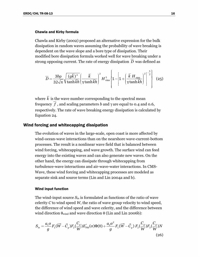
Chawla and Kirby formula
Chawla and Kirby (2002) proposed an alternative expression for the bulk dissipation in random waves assuming the probability of wave breaking is dependent on the wave slope and a bore type of dissipation. Their modified bore dissipation formula worked well for wave breaking under a strong opposing current. The rate of energy dissipation D was defined as
rmsrms
ρ ( )
tanh γ tanh γ tanhπ
k Hb gk kD H
kh kh kh
−⎧ ⎫⎪ ⎪⎪ ⎪⎡ ⎤⎛ ⎞⎛ ⎞ ⎪ ⎪⎢ ⎥⎟⎟ ⎪ ⎪⎪ ⎜ ⎪⎜ ⎟⎟= − +⎜⎜ ⎨ ⎬⎢ ⎥⎟⎟ ⎜⎜ ⎟⎟⎟ ⎪ ⎪⎟⎜ ⎜⎝ ⎠ ⎝ ⎠⎢ ⎥⎪ ⎪⎣ ⎦⎪ ⎪⎪ ⎪⎪ ⎪⎩ ⎭
522 23
53 1 132
(25)
where k is the wave number corresponding to the spectral mean
frequency f , and scaling parameters b and γ are equal to 0.4 and 0.6,
respectively. The rate of wave breaking energy dissipation is calculated by Equation 24.
Wind forcing and whitecapping dissipation
The evolution of waves in the large-scale, open coast is more affected by
wind-ocean-wave interactions than on the nearshore wave-current-bottom
processes. The result is a nonlinear wave field that is balanced between
wind forcing, whitecapping, and wave growth. The surface wind can feed
energy into the existing waves and can also generate new waves. On the
other hand, the energy can dissipate through whitecapping from
turbulence-wave interactions and air-wave-water interactions. In CMS-
Wave, these wind forcing and whitecapping processes are modeled as
separate sink and source terms (Lin and Lin 2004a and b).
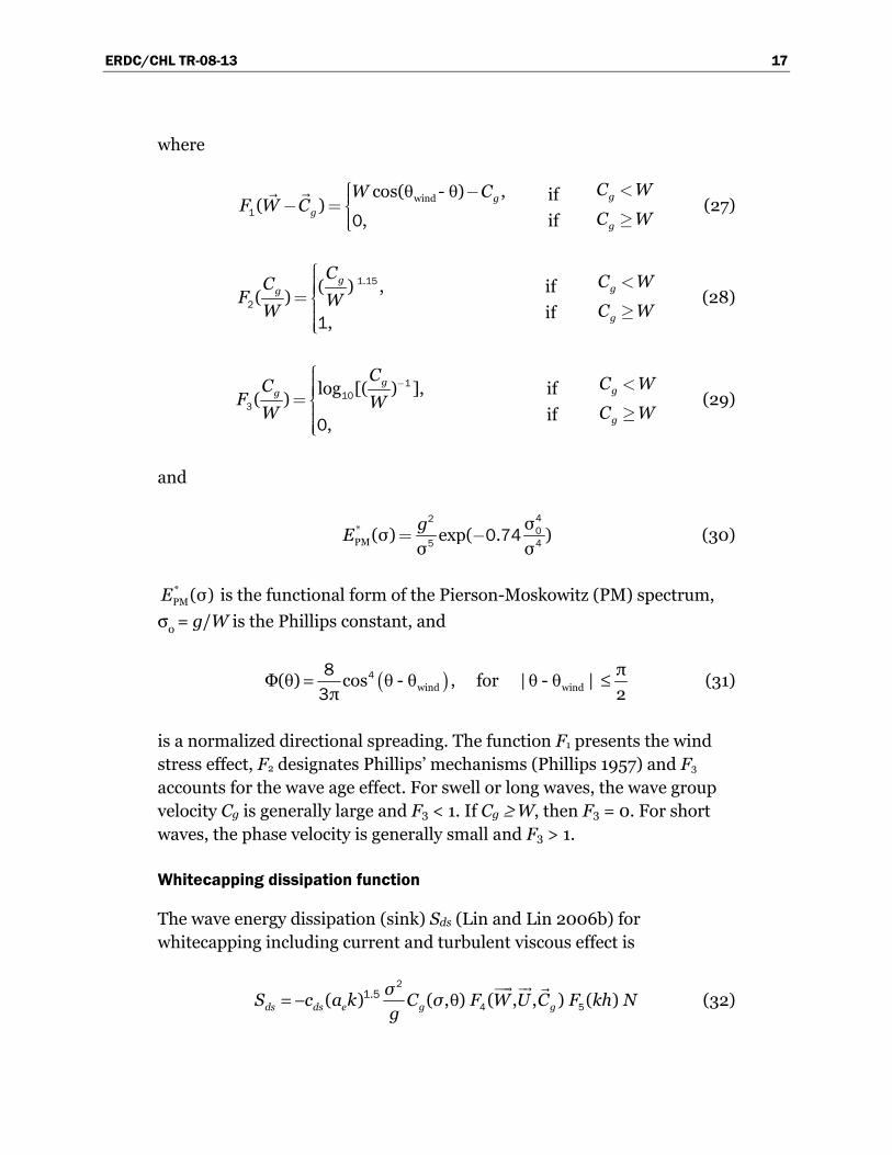
Wind input function
The wind-input source Sin is formulated as functions of the ratio of wave celerity C to wind speed W, the ratio of wave group velocity to wind speed, the difference of wind speed and wave celerity, and the difference between wind direction θwind and wave direction θ (Lin and Lin 2006b):
*PM θ
σ σ( ) ( ) (σ)Φ( ) ( ) ( ) ( )g g g
in g g
C C Ca aS F W C F E F W C F F N
g W g W W= − + −
21 2
1 2 1 2 3
(26)
ERDC/CHL TR-08-13 17
where
windθ θcos( - ) ,( )
,g
g
W CF W C
⎧ −⎪⎪− =⎨⎪⎪⎩1 0
if
if
g
g
C W
C W
<
≥ (27)
.( ) ,
( )
,
gg
CC
F WW
⎧⎪⎪⎪⎪=⎨⎪⎪⎪⎪⎩
1 15
2
1
if
if
g
g
C W
C W
<
≥ (28)
log [( ) ],
( )
,
gg
CC
F WW
−⎧⎪⎪⎪⎪=⎨⎪⎪⎪⎪⎩
110
3
0
if
if
g
g
C W
C W
<
≥ (29)
and
*PM
σ(σ) exp( . )
σ σg
E = −420
5 40 74 (30)
*PM(σ)E is the functional form of the Pierson-Moskowitz (PM) spectrum,
σo = g/W is the Phillips constant, and
( )= windθ θ θΦ( ) cos - π
483
, for | windθ θ- | π
2≤ (31)
is a normalized directional spreading. The function F1 presents the wind stress effect, F2 designates Phillips’ mechanisms (Phillips 1957) and F3 accounts for the wave age effect. For swell or long waves, the wave group velocity Cg is generally large and F3 < 1. If Cg ≥ W, then F3 = 0. For short waves, the phase velocity is generally small and F3 > 1.
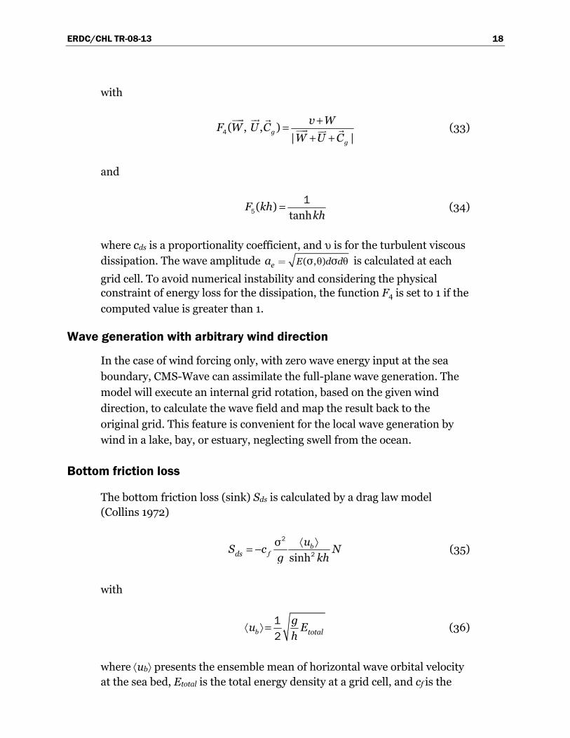
Whitecapping dissipation function
The wave energy dissipation (sink) Sds (Lin and Lin 2006b) for whitecapping including current and turbulent viscous effect is
= − . θ( ) ( , ) ( , , ) ( ) ds ds e g g
σS c a k C σ F W U C F kh N
g
2
4 51 5 (32)
ERDC/CHL TR-08-13 18
with
+=
+ +( , , )
| |g
g
v WF W U C
W U C4 (33)
and
( )tanh
F khkh5
1= (34)
where cds is a proportionality coefficient, and υ is for the turbulent viscous dissipation. The wave amplitude ( ,θ) θσ σe E d da = is calculated at each
grid cell. To avoid numerical instability and considering the physical constraint of energy loss for the dissipation, the function F4 is set to 1 if the
computed value is greater than 1.
Wave generation with arbitrary wind direction
In the case of wind forcing only, with zero wave energy input at the sea
boundary, CMS-Wave can assimilate the full-plane wave generation. The
model will execute an internal grid rotation, based on the given wind
direction, to calculate the wave field and map the result back to the
original grid. This feature is convenient for the local wave generation by
wind in a lake, bay, or estuary, neglecting swell from the ocean.
Bottom friction loss
The bottom friction loss (sink) Sds is calculated by a drag law model (Collins 1972)
σ
sinhb
fds
uS c N
g kh
2
2
⟨ ⟩= − (35)
with
⟨ ⟩=b total
gu E
h12
(36)
where ⟨ub⟩ presents the ensemble mean of horizontal wave orbital velocity at the sea bed, Etotal is the total energy density at a grid cell, and cf is the
ERDC/CHL TR-08-13 19
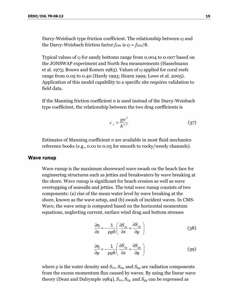
Darcy-Weisbach type friction coefficient. The relationship between cf and the Darcy-Weisbach friction factor fDW is cf = fDW/8.
Typical values of cf for sandy bottoms range from 0.004 to 0.007 based on the JONSWAP experiment and North Sea measurements (Hasselmann et al. 1973; Bouws and Komen 1983). Values of cf applied for coral reefs range from 0.05 to 0.40 (Hardy 1993; Hearn 1999; Lowe et al. 2005). Application of this model capability to a specific site requires validation to field data.
If the Manning friction coefficient n is used instead of the Darcy-Weisbach type coefficient, the relationship between the two drag coefficients is
2
1/3=fgnch
(37)
Estimates of Manning coefficient n are available in most fluid mechanics reference books (e.g., 0.01 to 0.05 for smooth to rocky/weedy channels).
Wave runup
Wave runup is the maximum shoreward wave swash on the beach face for engineering structures such as jetties and breakwaters by wave breaking at the shore. Wave runup is significant for beach erosion as well as wave overtopping of seawalls and jetties. The total wave runup consists of two components: (a) rise of the mean water level by wave breaking at the shore, known as the wave setup, and (b) swash of incident waves. In CMS-Wave, the wave setup is computed based on the horizontal momentum equations, neglecting current, surface wind drag and bottom stresses
η
ρxyxx
SS
x gh x y
1 ∂⎛ ⎞∂∂ = − +⎜ ⎟∂ ∂ ∂⎝ ⎠ (38)
η
ρxy yyS S
y gh x y
1 ∂ ∂⎛ ⎞∂ = − +⎜ ⎟∂ ∂ ∂⎝ ⎠ (39)
where ρ is the water density and Sxx, Sxy, and Syy are radiation components from the excess momentum flux caused by waves. By using the linear wave theory (Dean and Dalrymple 1984), Sxx, Sxy, and Syy can be expressed as
ERDC/CHL TR-08-13 20
θ) θ θ(σ, (cos )xx kS E n d2 112
⎡ ⎤= + −⎢ ⎥⎣ ⎦∫ (40)
θ θ θ(σ, ) (sin )xx kS E n d2 112
⎡ ⎤= + −⎢ ⎥⎣ ⎦∫ (41)
= θsinyy k
ES n 2
2 (42)
where = +sinhk
khn
kh
12
. Equations 38 and 39 also calculate the water level
depression from the still-water level resulting from waves known as wave setdown outside the breaker zone. Because CMS-Wave is a half-plane model, Equation 38 controls mainly wave setup and setdown calculations, whereas Equation 39 acts predominantly to smooth the water level alongshore.
The swash oscillation of incident natural waves on the beach face is a random process. The most landward swash excursion corresponds to the maximum wave runup. In the engineering application, a 2% exceedance of all vertical levels, denoted as R2, from the swash is usually estimated for the wave runup (Komar 1998). This quantity is approximately equal to the local wave setup on the beach or at structures such as seawalls and jetties, or the total wave runup is estimated as
max2 2 ηR = (43)
In CMS-Wave, R2 is calculated at the land-water interface and averaged with the local depth to determine if the water can flood the proceeding dry cell. If the wave runup level is higher than the adjacent land cell elevation, CMS-Wave can flood the dry cells and simulate wave overtopping and overwash at them. The feature is useful in coupling CMS-Wave to CMS-Flow (Buttolph et al. 2006) for calculating beach erosion or breaching. Calculated quantities of ∂Sxx/∂x, ∂Sxy/∂x, ∂Sxy/∂y, and ∂Syy/∂y are saved as input to CMS-Flow. CMS-Wave reports the calculated fields of wave setup and maximum water level defined as
Maximum water level = Max (R2, η + H1/3/2) (44)
ERDC/CHL TR-08-13 21
Wave transmission and overtopping at structures
CMS-Wave applies a simple analytical formula to compute the wave transmission coefficient Kt of a rigidly moored rectangular breakwater of width Bc and draft Dc (Macagno 1953)
−⎡ ⎤⎛ ⎞⎢ ⎥⎜ ⎟⎢ ⎥= + ⎜ ⎟−⎢ ⎥⎜ ⎟⎜ ⎟⎢ ⎥⎝ ⎠⎣ ⎦
sinhπ
cosh ( )
c
tc
khkB
Kk h D
12 2
212
(45)
Wave transmission over a structure or breakwater is caused mainly by the fall of the overtopping water mass. Therefore, the ratio of the structure crest elevation to the incident wave height is the prime parameter governing the wave transmission. CMS calculates the rate of overtopping of a vertical breakwater based on the simple expression (Goda 1985) as
= − ≤ ≤. ( . ), for .c ct
i i
h hK
H H0 3 1 5 0 1 25 (46)
where hc is the crest elevation of the breakwater above the still-water level, and Hi is the incident wave height. Equation 46 is modified for a composite breakwater, protected by a mound of armor units at its front, as
= − ≤ ≤. ( . ), for .c ct
i i
h hK
H H0 3 1 1 0 0 75 (47)
For rubble-mound breakwaters, the calculation of wave transmission is more complicated because the overtopping rate also depends on the specific design of the breakwater (e. g., toe apron protection, front slope, armor unit shape and size, thickness of armor layers). In practice, Equation 47 still can be applied using a finer spatial resolution with the proper bathymetry and adequate bottom friction coefficients to represent the breakwater.
Grid nesting
Grid nesting is applied by saving wave spectra at selected locations from a
coarse grid (parent grid) and inputting them along the offshore boundary
of the smaller fine grid (child grid). For simple and quick applications, a
single-location spectrum saved from the parent grid can be used as the
ERDC/CHL TR-08-13 22
wave forcing for the entire sea boundary of the child grid. If multi-location
spectra were saved from the parent grid, they are then interpolated as well
as extrapolated for more realistic wave forcing along the sea boundary of
the child grid.
Multiple grid nesting (e.g., several co-existing child grids and grandchild
grids) is supported by CMS-Wave. The parent and child grids can have
different orientations, but need to reside in the same horizontal coordinate
system. Because CMS-Wave is a half-plane model, the difference between
grid orientations between parent and child grids should be small (no
greater than 45 deg) for passing sufficient wave energy from the parent to
child grids.
Variable-rectangular-cell grid
CMS-Wave can run on a grid with variable rectangular cells. This feature is
suited to large-domain applications in which wider spacing cells can be
specified in the offshore, where wave property variation is small and away
from the area of interest, to save computational time. A limit on the shore-
normal to shore-parallel spacing ratio in a cell is not required as long as
the calculated shoreward waves are found to be numerically stable.
Non-linear wave-wave interaction
Non-linear wave-wave interactions are a conserved energy transfer from
higher to lower frequencies. They can produce transverse waves and
energy diffusion in the frequency and direction domains. The effect is
more pronounced in shallower water. Directional spreading of the wave
spectrum tends to increase as the wavelength decreases.
The exact computation of the nonlinear energy transfer involves six-
dimensional integrations. This is computationally too taxing to be used in
practical engineering nearshore wave transformation models. Mase et al.
(2005a) have shown that calculated wave fields differ with and without
nonlinear energy transfer. Jenkins and Phillips (2001) proposed a simple
formula as an approximation of the nonlinear wave-wave interaction.
Testing of this formula in CMS-Wave is underway.
ERDC/CHL TR-08-13 23
Fast-mode calculation
CMS-Wave can run in a fast mode for simple and quick applications. The
fast mode calculates the half-plane spectral transformation on either five
directional bins (each 30-deg angle for a broad-band input spectrum) or
seven directional bins (each 5-deg angle for a narrow-band input spectrum
or 25-deg angle with wind input) to minimize simulation time. It runs at
least five times faster than the normal mode, which operates with 35
directional bins. The fast-mode option is suited for a long or time-pressing
simulation if users are seeking preliminary solutions. The wave direction
estimated in the fast mode is expected to be less accurate than the
standard mode because the directional calculation is based on fewer bins.
ERDC/CHL TR-08-13 24
3 CMS-Wave Interface
Demirbilek et al. (2007) described the computer graphical interface in the SMS (Zundel 2006) for CMS-Wave applications. A summary of key features of the interface is provided in this chapter to familiarize users with guidelines for the interface usage and implementation of CMS-Wave. The SMS is a graphically interactive computer program designed to facilitate the operation of numerical models and creates input files and output visualization for CMS-Wave. The CMS-Wave interface in the SMS is similar to that of the half-plane model of STWAVE Version 5.4 (Smith 2001b). The SMS can generate CMS grids with variable rectangle cells and half-plane STWAVE grids with constant square cells. Both wave models can use the same grid domain with identical grid orientation and layout, and the same file formats for their bathymetric and spectral energy files. This was done to facilitate the usage of CMS-Wave and allow users to utilize the same settings and files to run both models without modifications.
CMS-Wave files
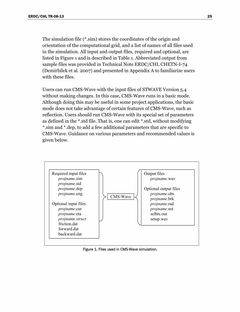
Four input files are required for a CMS-Wave simulation (Figure 1): the simulation file (*.sim), the model parameters file (*.std), the depth file (*.dep), and the input directional spectrum file (*.eng). Optional input files include a current field file (*.cur), a water level field file (*.eta), a friction coefficient field (friction.dat), a forward reflection coefficient field (forward.dat), a backward reflection coefficient field (backward.dat), and a structure file (*.struct). The name of the simulation file can be passed to CMS-Wave as a command line argument, or the program will prompt the user for this file. The model can be launched in the SMS or at a DOS prompt by specifying the name of the simulation file (*.sim).
Depending on which options are selected in the *.std file, CMS-Wave may generate one to six output files. A wave field conditions file (*.wav) is always generated. Optional output files are calculated spectra (*.obs) and wave parameters with the maximum water level (selhts.out) at selected cells, wave breaking indices (*.brk), wave radiation stress gradients (*.rad), wave setup and maximum water level field (setup.wav), and nesting spectral data (*.nst). Figure 1 shows a chart of input and output files involved in a CMS-Wave simulation. Table 1 presents a list of the type and use of all I/O files, where “projname” is a prefix given by users.
ERDC/CHL TR-08-13 25
The simulation file (*.sim) stores the coordinates of the origin and orientation of the computational grid, and a list of names of all files used in the simulation. All input and output files, required and optional, are listed in Figure 1 and is described in Table 1. Abbreviated output from sample files was provided in Technical Note ERDC/CHL CHETN-I-74 (Demirbilek et al. 2007) and presented in Appendix A to familiarize users with these files.
Users can run CMS-Wave with the input files of STWAVE Version 5.4 without making changes. In this case, CMS-Wave runs in a basic mode. Although doing this may be useful in some project applications, the basic mode does not take advantage of certain features of CMS-Wave, such as reflection. Users should run CMS-Wave with its special set of parameters as defined in the *.std file. That is, one can edit *.std, without modifying *.sim and *.dep, to add a few additional parameters that are specific to CMS-Wave. Guidance on various parameters and recommended values is given below.
Figure 1. Files used in CMS-Wave simulation.
CMS-Wave
Required input files projname.sim projname.std projname.dep projname.eng Optional input files projname.cur projname.eta projname.struct friction.dat forward.dat backward.dat
Output files projname.wav Optional output files projname.obs projname.brk projname.rad projname.nst selhts.out setup.wav
ERDC/CHL TR-08-13 26
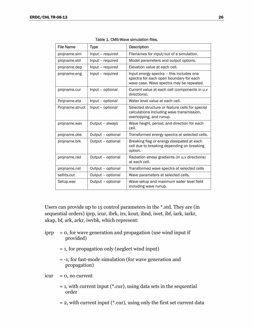
Table 1. CMS-Wave simulation files.
File Name Type Description
projname.sim Input – required Filenames for input/out of a simulation. projname.std Input – required Model parameters and output options. projname.dep Input – required Elevation value at each cell. projname.eng Input – required Input energy spectra – this includes one
spectra for each open boundary for each wave case. Wave spectra may be repeated.
projname.cur Input – optional Current value at each cell (components in u,v directions).
Projname.eta Input – optional Water level value at each cell. Projname.struct Input – optional Selected structure or feature cells for special
calculations including wave transmission, overtopping, and runup.
projname.wav Output – always Wave height, period, and direction for each cell.
projname.obs Output – optional Transformed energy spectra at selected cells. projname.brk Output – optional Breaking flag or energy dissipated at each
cell due to breaking depending on breaking option.
projname.rad Output – optional Radiation stress gradients (in u,v directions) at each cell.
projname.nst Output – optional Transformed wave spectra at selected cells selhts.out Output – optional Wave parameters at selected cells. Setup.wav Output – optional Wave setup and maximum water level field
including wave runup.
Users can provide up to 15 control parameters in the *.std. They are (in sequential orders) iprp, icur, ibrk, irs, kout, ibnd, iwet, ibf, iark, iarkr, akap, bf, ark, arkr, iwvbk, which represent:
iprp = 0, for wave generation and propagation (use wind input if provided)
= 1, for propagation only (neglect wind input)
= -1, for fast-mode simulation (for wave generation and propagation)
icur = 0, no current
= 1, with current input (*.cur), using data sets in the sequential order
= 2, with current input (*.cur), using only the first set current data
ERDC/CHL TR-08-13 27
ibrk = 0 (no *.brk file)
= 1, for output of wave breaking indices (*.brk)
= 2, for output of energy dissipation fluxes (*.brk)
irs = 0 (no *.rad file)
= 1, for output of wave radiation stresses (*.rad)
= 2, for output of wave radiation stresses (*.rad) and wave setup/maximum water level (setup.wav)
kout = 0 (no *.obs and selhts.out files)
= n, for output of spectra (*.obs) and parameters (selhts.out) at n selected cells
ibnd = 0 (no *.nst file)
= 1, for nested grid, with linear interpolation of boundary input spectra (*.nst)
= 2, for nested grid, with morphic interpolation of boundary input spectra (*.nst)
iwet = 0, for normal wetting/drying (use water level input)
= 1, no wetting/drying (neglect water level input)
ibf = 0, no bottom friction
= 1, for bottom friction with constant Darcy-Weisbach type coefficient (= bf)
= 2, for bottom friction with variable Darcy-Weisbach type coefficient (friction.dat)
= 3, for bottom friction with constant Manning coefficient (= bf)
= 4, for bottom friction with variable Manning coefficient (friction.dat)
iark = 0, no forward reflection
= 1, with forward reflection
iarkr = 0, no backward reflection
= 1, for backward reflection
ERDC/CHL TR-08-13 28
akap = diffraction intensity factor (0 for no diffraction, 4 for strong diffraction)
bf = constant bottom friction coefficient
ark = constant forward reflection coefficient (0 for no reflection, 1 for maximum forward reflection)
arkr = constant backward reflection coefficient (0 for no reflection, 1 for maximum backward reflection)
iwvbk = option for selection of wave breaking formula
= 0, for Extended Goda (Sakai et al. 1989)
= 1, for Extended Miche (Battjes 1972; Mase et al. 2005b)
= 2, for formula by Battjes and Janssen (1978)
= 3, for formula by Chawla and Kirby (2002)
Users can assign 0 for 15 control parameters in CMS-Wave to run in the basic mode. If only the first six parameters, iprp, icur, ibrk, irs, kout, and ibnd, are provided (minimum requirement) in *.std, a zero will be assigned to the remaining parameters, except that a default value of 1.0 is assigned to the diffraction intensity factor (akap = 1.0) to simulate a weak diffraction condition. If only the first ten parameters, iprp, icur, ibrk, irs, kout, ibnd, iwet, ibf, iark, and iarkr, are provided in *.std (no other information provided for the bottom friction and reflection coefficients), default values of bf = 0.0, ark = 0.5 (for 50 percent energy forward reflection), arkr = 0.3 (for 30 percent backward energy reflection), and akap = 1.0 are used by the model.
CMS-Wave calculates wave transmission, wave runup, and overtopping as special features on selected cells. These cells can represent a floating breakwater, a bottom mound breakwater, a beach segment and the land adjacent to it, jetties, seawalls, or underwater features such as reefs or submerged structures. A trench, submerged mound, or structure can be added to the bed as features without modifying the input depth file. These feature cells need to be specified in the *.struct file. Each feature cell is described by four parameters, istruc, jstruc, kstruc, and cstruc in a line format in the *.struct.
istruc = i-th column in the grid
ERDC/CHL TR-08-13 29
jstruc = j-th row in the grid
kstruc = feature cell identity
= 1, for adding alternative feature or structure (immersed or exposed) without modifying the input depth
= 2, for calculation of wave runup and overwash on beach face or structure, and adjacent land
= 3, for calculation of transmitted waves of a floating breakwater
= 4, for a vertical wall breakwater
= 5, for a composite or rubble-mound breakwater
cstruc = feature structure depth, for kstruc = 1 (assume a land cell if not provided)
= beach/structure elevation above mean water level, for kstruc = 2 (use the input depth if not provided; no effect for cstruc < 0)
= floating breakwater draft, for kstruc =3 (skip if not provided or cstruc < 0.05 m)
= breakwater/structure elevation, for kstruc = 4 or 5 (use the input depth if not provided; immersed if cstruc < 0)
Components of CMS-Wave interface
The interface for CMS-Wave is designed for the half-plane, i.e., 180-deg sector where waves propagate from offshore toward the shoreline. Similar to other finite-difference models available in the SMS, CMS-Wave is controlled through the 2D Cartesian Grid Module . The user should select the Set Current Model command in the Edit menu and choose CMS-Wave to activate the model interface. After CMS-Wave is selected as the active model, its menu and tools become available. It is recommended that users become familiar with other modules of the SMS to fully exploit the complete utility of the interface. For example, the CMS-Wave grid can also be generated in the Map Module under the CMS-Wave coverage. Likewise, users can select the Scatter Module to import survey data and digital maps to define the bathymetry for the model’s grids.
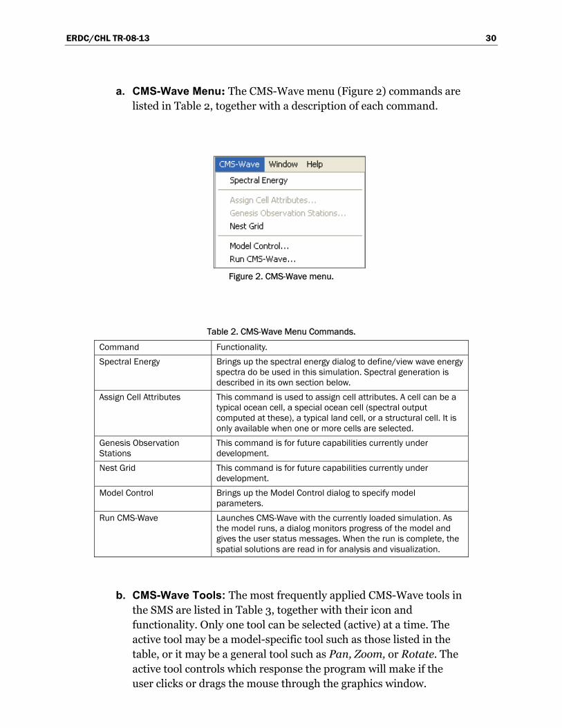
ERDC/CHL TR-08-13 30
a. CMS-Wave Menu: The CMS-Wave menu (Figure 2) commands are listed in Table 2, together with a description of each command.
Figure 2. CMS-Wave menu.
Table 2. CMS-Wave Menu Commands.
Command Functionality. Spectral Energy Brings up the spectral energy dialog to define/view wave energy
spectra do be used in this simulation. Spectral generation is described in its own section below.
Assign Cell Attributes This command is used to assign cell attributes. A cell can be a typical ocean cell, a special ocean cell (spectral output computed at these), a typical land cell, or a structural cell. It is only available when one or more cells are selected.
Genesis Observation Stations
This command is for future capabilities currently under development.
Nest Grid This command is for future capabilities currently under development.
Model Control Brings up the Model Control dialog to specify model parameters.
Run CMS-Wave Launches CMS-Wave with the currently loaded simulation. As the model runs, a dialog monitors progress of the model and gives the user status messages. When the run is complete, the spatial solutions are read in for analysis and visualization.
b. CMS-Wave Tools: The most frequently applied CMS-Wave tools in the SMS are listed in Table 3, together with their icon and functionality. Only one tool can be selected (active) at a time. The active tool may be a model-specific tool such as those listed in the table, or it may be a general tool such as Pan, Zoom, or Rotate. The active tool controls which response the program will make if the user clicks or drags the mouse through the graphics window.
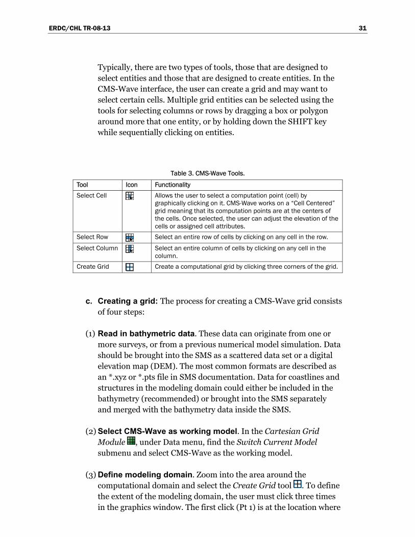
ERDC/CHL TR-08-13 31
Typically, there are two types of tools, those that are designed to select entities and those that are designed to create entities. In the CMS-Wave interface, the user can create a grid and may want to select certain cells. Multiple grid entities can be selected using the tools for selecting columns or rows by dragging a box or polygon around more that one entity, or by holding down the SHIFT key while sequentially clicking on entities.
Table 3. CMS-Wave Tools.
Tool Icon Functionality Select Cell Allows the user to select a computation point (cell) by
graphically clicking on it. CMS-Wave works on a “Cell Centered” grid meaning that its computation points are at the centers of the cells. Once selected, the user can adjust the elevation of the cells or assigned cell attributes.
Select Row Select an entire row of cells by clicking on any cell in the row.
Select Column Select an entire column of cells by clicking on any cell in the column.
Create Grid Create a computational grid by clicking three corners of the grid.
c. Creating a grid: The process for creating a CMS-Wave grid consists of four steps:
(1) Read in bathymetric data. These data can originate from one or more surveys, or from a previous numerical model simulation. Data should be brought into the SMS as a scattered data set or a digital elevation map (DEM). The most common formats are described as an *.xyz or *.pts file in SMS documentation. Data for coastlines and structures in the modeling domain could either be included in the bathymetry (recommended) or brought into the SMS separately and merged with the bathymetry data inside the SMS.
(2) Select CMS-Wave as working model. In the Cartesian Grid Module , under Data menu, find the Switch Current Model submenu and select CMS-Wave as the working model.
(3) Define modeling domain. Zoom into the area around the computational domain and select the Create Grid tool . To define the extent of the modeling domain, the user must click three times in the graphics window. The first click (Pt 1) is at the location where
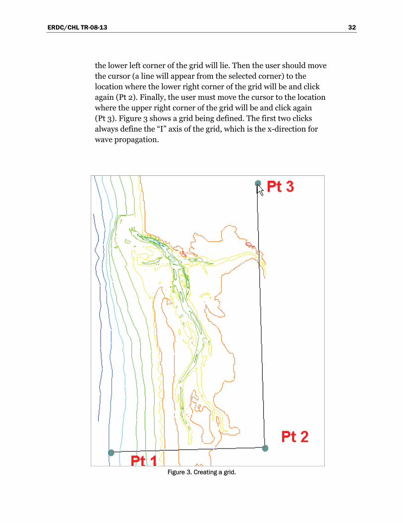
ERDC/CHL TR-08-13 32
the lower left corner of the grid will lie. Then the user should move the cursor (a line will appear from the selected corner) to the location where the lower right corner of the grid will be and click again (Pt 2). Finally, the user must move the cursor to the location where the upper right corner of the grid will be and click again (Pt 3). Figure 3 shows a grid being defined. The first two clicks always define the “I” axis of the grid, which is the x-direction for wave propagation.
Figure 3. Creating a grid.
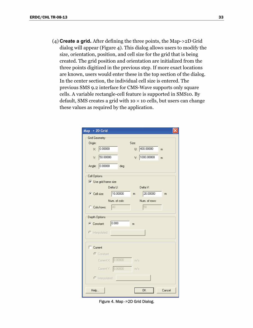
ERDC/CHL TR-08-13 33
(4) Create a grid. After defining the three points, the Map->2D Grid dialog will appear (Figure 4). This dialog allows users to modify the size, orientation, position, and cell size for the grid that is being created. The grid position and orientation are initialized from the three points digitized in the previous step. If more exact locations are known, users would enter these in the top section of the dialog. In the center section, the individual cell size is entered. The previous SMS 9.2 interface for CMS-Wave supports only square cells. A variable rectangle-cell feature is supported in SMS10. By default, SMS creates a grid with 10 × 10 cells, but users can change these values as required by the application.
Figure 4. Map ->2D Grid Dialog.
ERDC/CHL TR-08-13 34
In the lower section of this dialog, users tell the SMS to interpolate the bathymetry values for the grid from the data resident in the Scatter Module. If a scattered data set with a vector functional data set exists in the SMS at the time the grid is created, there is also an option to interpolate current data to the grid. Once this data set is entered, the user clicks the OK button, and a grid is created. Bathymetry values for each cell of the grid, along with values of the horizontal current, are interpolated from the scattered bathymetry data at the centroid of the cells. Grid cells with a negative depth value are classified as dry land and are excluded in the CMS-Wave calculations. After the grid is created, the user can select cells and modify depth values and cell classifications (type).
d. Editing a grid: Cell depths and attributes in the CMS-Wave grid may be edited, but the grid itself cannot be repositioned. To reposition or change the resolution of a grid, a new grid must be created. This is required if the domain needs to be enlarged or reduced, the grid cell size modified, or the grid orientation adjusted to align it better with the principal wave direction. Various other types of operation are permitted for editing CMS-Wave grid cells, including the following:
(1) Specification of individual cell elevation. Select one or more cells using the Select Cell tool , and specify a elevation value in the edit field located at the top of the application (just below the menus). This feature could be used, for example, to evaluate the response of waves to dredging operations by deepening parts of a navigation channel or to describe dredged material mounds in the modeling domain. This feature is useful if some changes to the underlying bathymetry are desired in a small part of the modeling domain where they can be made manually to a sub-area or selection of cells.
(2) Classification of cell as land, structure, water, or monitoring (special output) location. This is done by selecting one or more cells using the Select Cell tool and specifying the cell attributes using the Assign Cell Attributes command in the menu. This brings up the Cell Attributes dialog.
e. Monitoring Cells: The SMS interface for CMS-Wave allows for the monitoring of certain cells in the computational domain. To do this, users simply select the cells, as described above in the section on
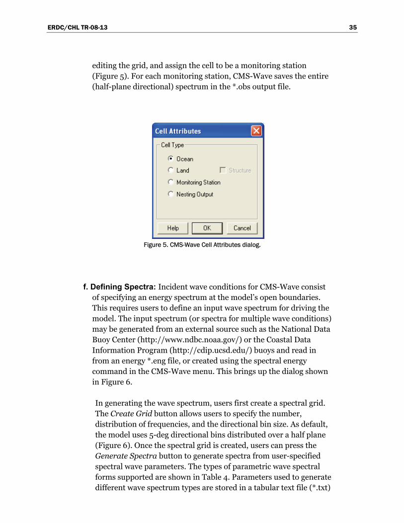
ERDC/CHL TR-08-13 35
editing the grid, and assign the cell to be a monitoring station (Figure 5). For each monitoring station, CMS-Wave saves the entire (half-plane directional) spectrum in the *.obs output file.
Figure 5. CMS-Wave Cell Attributes dialog.
f. Defining Spectra: Incident wave conditions for CMS-Wave consist of specifying an energy spectrum at the model’s open boundaries. This requires users to define an input wave spectrum for driving the model. The input spectrum (or spectra for multiple wave conditions) may be generated from an external source such as the National Data Buoy Center (http://www.ndbc.noaa.gov/) or the Coastal Data Information Program (http://cdip.ucsd.edu/) buoys and read in from an energy *.eng file, or created using the spectral energy command in the CMS-Wave menu. This brings up the dialog shown in Figure 6.
In generating the wave spectrum, users first create a spectral grid. The Create Grid button allows users to specify the number, distribution of frequencies, and the directional bin size. As default, the model uses 5-deg directional bins distributed over a half plane (Figure 6). Once the spectral grid is created, users can press the Generate Spectra button to generate spectra from user-specified spectral wave parameters. The types of parametric wave spectral forms supported are shown in Table 4. Parameters used to generate different wave spectrum types are stored in a tabular text file (*.txt)
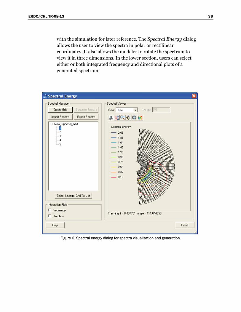
ERDC/CHL TR-08-13 36
with the simulation for later reference. The Spectral Energy dialog allows the user to view the spectra in polar or rectilinear coordinates. It also allows the modeler to rotate the spectrum to view it in three dimensions. In the lower section, users can select either or both integrated frequency and directional plots of a generated spectrum.
Figure 6. Spectral energy dialog for spectra visualization and generation.
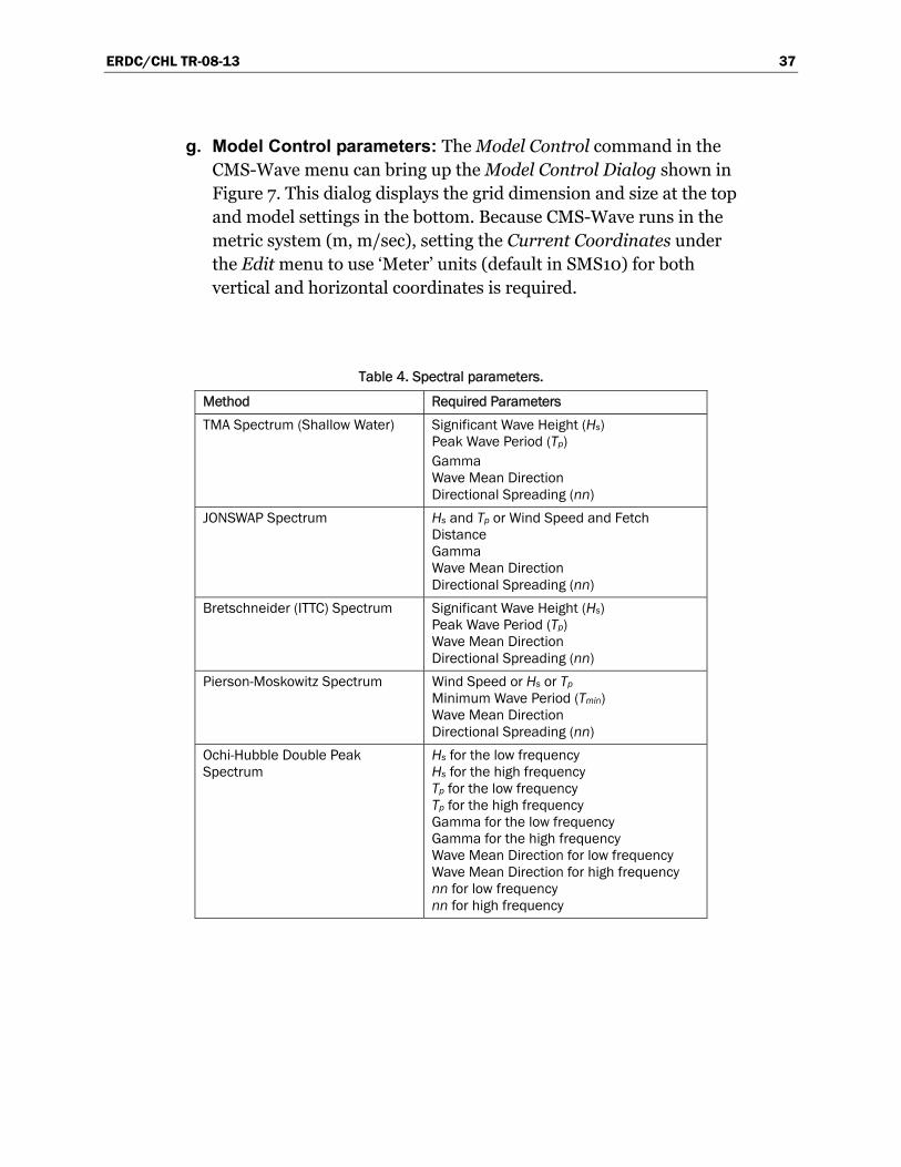
ERDC/CHL TR-08-13 37
g. Model Control parameters: The Model Control command in the CMS-Wave menu can bring up the Model Control Dialog shown in Figure 7. This dialog displays the grid dimension and size at the top and model settings in the bottom. Because CMS-Wave runs in the metric system (m, m/sec), setting the Current Coordinates under the Edit menu to use ‘Meter’ units (default in SMS10) for both vertical and horizontal coordinates is required.
Table 4. Spectral parameters.
Method Required Parameters TMA Spectrum (Shallow Water) Significant Wave Height (Hs)
Peak Wave Period (Tp) Gamma Wave Mean Direction Directional Spreading (nn)
JONSWAP Spectrum Hs and Tp or Wind Speed and Fetch Distance Gamma Wave Mean Direction Directional Spreading (nn)
Bretschneider (ITTC) Spectrum Significant Wave Height (Hs) Peak Wave Period (Tp) Wave Mean Direction Directional Spreading (nn)
Pierson-Moskowitz Spectrum Wind Speed or Hs or Tp
Minimum Wave Period (Tmin) Wave Mean Direction Directional Spreading (nn)
Ochi-Hubble Double Peak Spectrum
Hs for the low frequency Hs for the high frequency Tp for the low frequency Tp for the high frequency Gamma for the low frequency Gamma for the high frequency Wave Mean Direction for low frequency Wave Mean Direction for high frequency nn for low frequency nn for high frequency
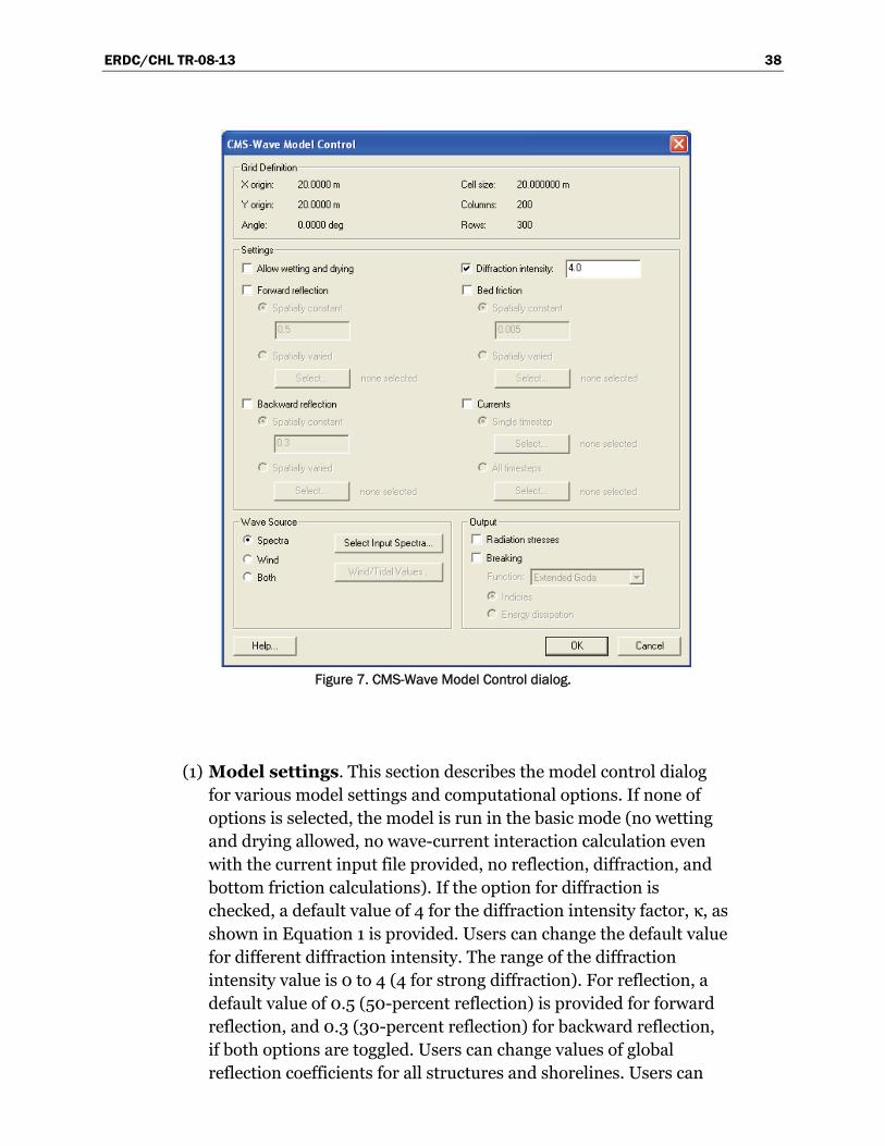
ERDC/CHL TR-08-13 38
Figure 7. CMS-Wave Model Control dialog.
(1) Model settings. This section describes the model control dialog for various model settings and computational options. If none of options is selected, the model is run in the basic mode (no wetting and drying allowed, no wave-current interaction calculation even with the current input file provided, no reflection, diffraction, and bottom friction calculations). If the option for diffraction is checked, a default value of 4 for the diffraction intensity factor, κ, as shown in Equation 1 is provided. Users can change the default value for different diffraction intensity. The range of the diffraction intensity value is 0 to 4 (4 for strong diffraction). For reflection, a default value of 0.5 (50-percent reflection) is provided for forward reflection, and 0.3 (30-percent reflection) for backward reflection, if both options are toggled. Users can change values of global reflection coefficients for all structures and shorelines. Users can
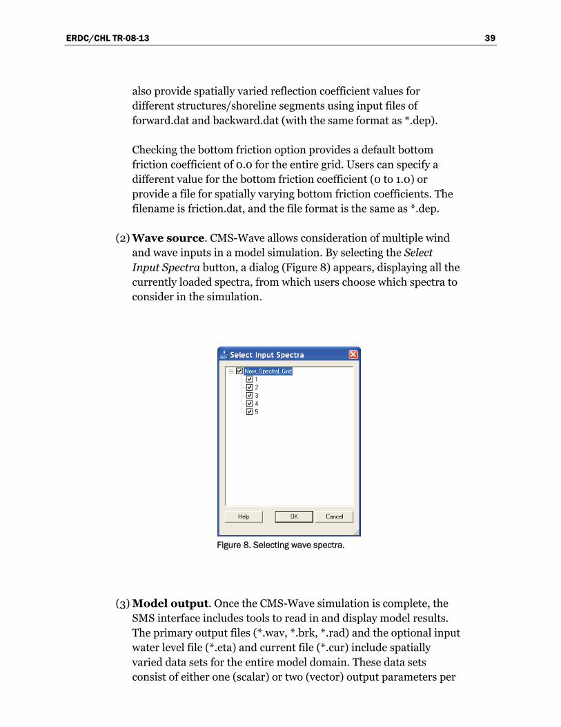
ERDC/CHL TR-08-13 39
also provide spatially varied reflection coefficient values for different structures/shoreline segments using input files of forward.dat and backward.dat (with the same format as *.dep).
Checking the bottom friction option provides a default bottom friction coefficient of 0.0 for the entire grid. Users can specify a different value for the bottom friction coefficient (0 to 1.0) or provide a file for spatially varying bottom friction coefficients. The filename is friction.dat, and the file format is the same as *.dep.
(2) Wave source. CMS-Wave allows consideration of multiple wind and wave inputs in a model simulation. By selecting the Select Input Spectra button, a dialog (Figure 8) appears, displaying all the currently loaded spectra, from which users choose which spectra to consider in the simulation.
Figure 8. Selecting wave spectra.
(3) Model output. Once the CMS-Wave simulation is complete, the SMS interface includes tools to read in and display model results. The primary output files (*.wav, *.brk, *.rad) and the optional input water level file (*.eta) and current file (*.cur) include spatially varied data sets for the entire model domain. These data sets consist of either one (scalar) or two (vector) output parameters per
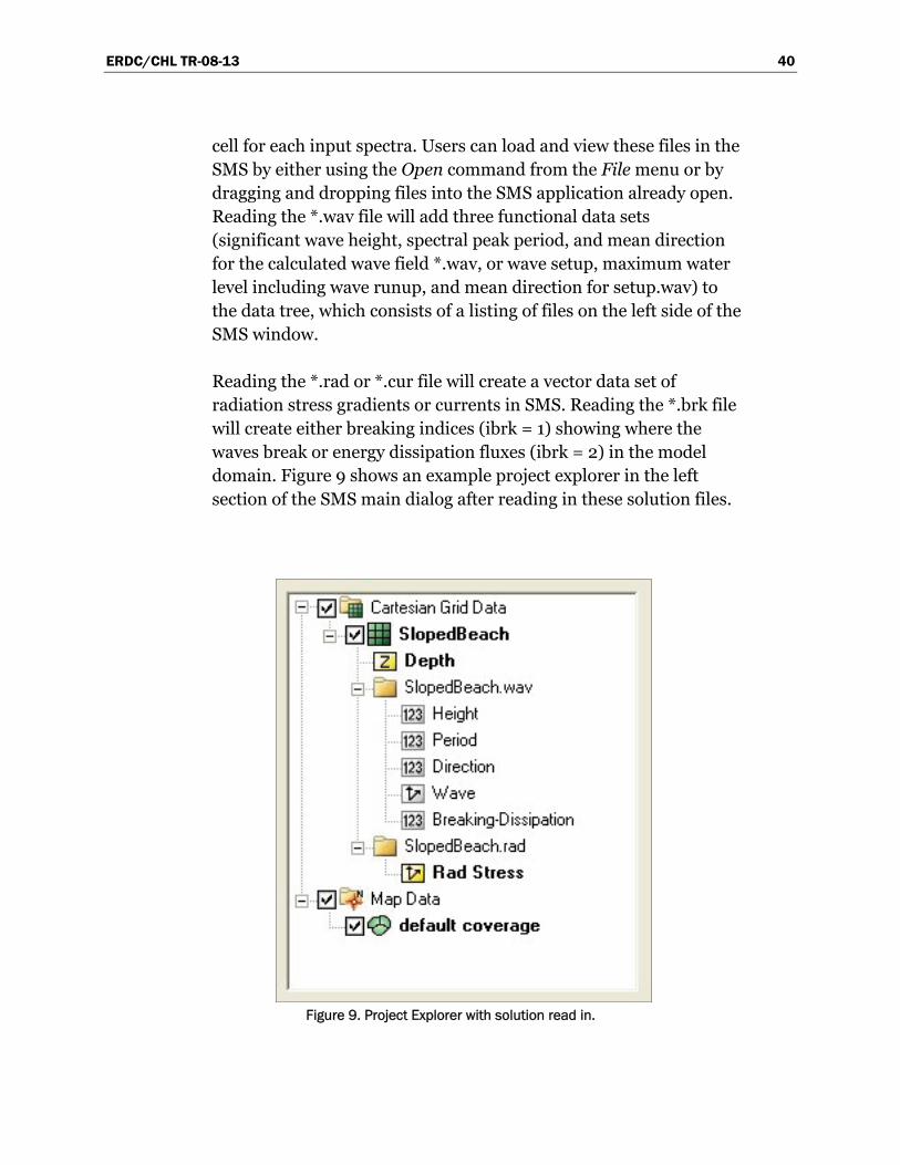
ERDC/CHL TR-08-13 40
cell for each input spectra. Users can load and view these files in the SMS by either using the Open command from the File menu or by dragging and dropping files into the SMS application already open. Reading the *.wav file will add three functional data sets (significant wave height, spectral peak period, and mean direction for the calculated wave field *.wav, or wave setup, maximum water level including wave runup, and mean direction for setup.wav) to the data tree, which consists of a listing of files on the left side of the SMS window.
Reading the *.rad or *.cur file will create a vector data set of radiation stress gradients or currents in SMS. Reading the *.brk file will create either breaking indices (ibrk = 1) showing where the waves break or energy dissipation fluxes (ibrk = 2) in the model domain. Figure 9 shows an example project explorer in the left section of the SMS main dialog after reading in these solution files.
Figure 9. Project Explorer with solution read in.
ERDC/CHL TR-08-13 41
The model control parameters are listed in the first line of the *.std file. There may be 6 to 15 parameters in the *.std file. The first six parameters are defined for running CMS-Wave in the same mode as the half-plane STWAVE Version 5.4. As was noted earlier, if a simulation is performed with only the first six parameters in the *.std file, this will not take advantage of CMS-Wave’s additional capabilities that are not available in STWAVE Version 5.4. The other nine parameters in the *.std file are special feature settings defined specifically for CMS-Wave. Under the CMS environment, users can use the same input files for CMS-Wave to run STWAVE Version 5.4 in the SMS by providing dummy values for the wave reflection and diffraction intensity parameters in the *.std file.
The SMS can display contours of the selected scalar or vector data sets for either input or output field data over the modeling domain. The *.obs file includes spectra computed by the model at the observation cells. These calculated spectra at the observation cells can be displayed and evaluated as the input spectra using the spectral energy dialog.
ERDC/CHL TR-08-13 42
4 Model Validation
Numerical models are validated by comparing model calculations to data and analytical solutions to determine the reliability of a model’s individual or combined features. Data for model validation come from laboratory and field measurements, whereas analytical solutions are available in the literature and engineering manuals. Validation tests are essential benchmarks for evaluating both general features and the unique capabilities of numerical models.
This chapter describes and discusses nine examples, or cases, and four depth-limited breaking wave formulas. The CMS-Wave validation is shown for eight data sets from laboratory and field studies, two sets of analytical solutions, and two sets of semi-empirical calculations. The laboratory data are from experiments that have been conducted for idealized inlets, plain sloping beaches, and jetties. These data are examined for validation of wave breaking formulas, wave-current interaction, wave runup, and overall model performance at inlets and nearshore. Theoretical solutions for wave diffraction at a semi-infinite breakwater, a single gap, and multiple gaps in breakwaters are examined to evaluate the reliability of CMS-Wave calculations for simulating wave-structure interaction problems. The wind-wave growth capability of CMS-Wave is validated with semi-empirical relations given in the U.S Army Corps of Engineers Shore Protection Manual (1984) and Coastal Engineering Manual (Headquarters (HQ), USACE 2002).
The wave reflection capability of CMS-Wave was tested based on a laboratory experiment conducted for an idealized inlet protected by dual jetties (Seabergh et al. 2005). Both fully reflected and absorbing jetties were tested in the experiment. Details of the experiment, data, and CMS-Wave predictions and comparisons were summarized in (Lin et al. 2006b). This Technical Note also includes additional tests comparing CMS-Wave results to data for wave diffraction around and behind a shore-parallel breakwater and wave diffraction measurements by Seabergh et al. (2002) at the bay side of an inlet.
Case 1: Wave shoaling and breaking around an idealized inlet
Smith et al. (1998) conducted a laboratory study to investigate the wave-current interaction and the associated wave breaking in an idealized
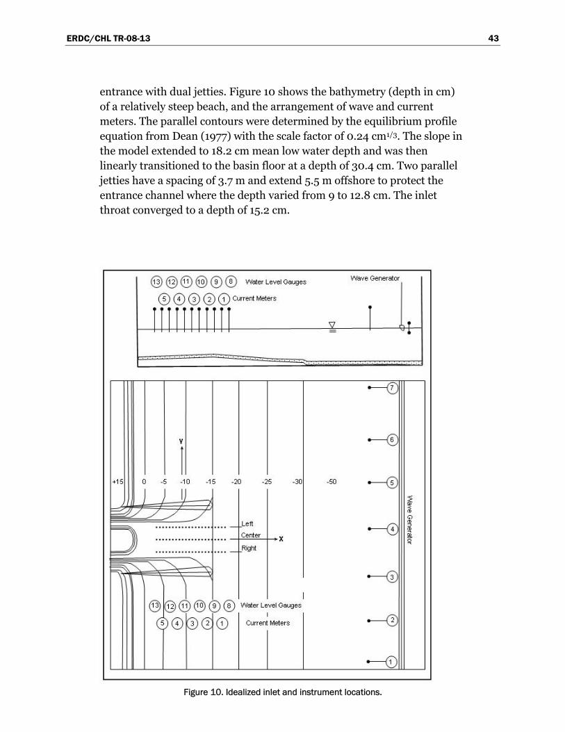
ERDC/CHL TR-08-13 43
entrance with dual jetties. Figure 10 shows the bathymetry (depth in cm) of a relatively steep beach, and the arrangement of wave and current meters. The parallel contours were determined by the equilibrium profile equation from Dean (1977) with the scale factor of 0.24 cm1/3. The slope in the model extended to 18.2 cm mean low water depth and was then linearly transitioned to the basin floor at a depth of 30.4 cm. Two parallel jetties have a spacing of 3.7 m and extend 5.5 m offshore to protect the entrance channel where the depth varied from 9 to 12.8 cm. The inlet throat converged to a depth of 15.2 cm.
Figure 10. Idealized inlet and instrument locations.
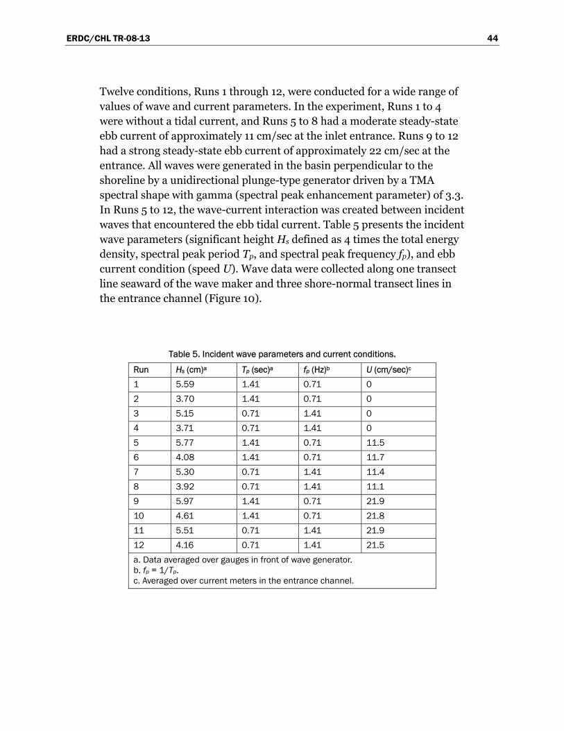
ERDC/CHL TR-08-13 44
Twelve conditions, Runs 1 through 12, were conducted for a wide range of values of wave and current parameters. In the experiment, Runs 1 to 4 were without a tidal current, and Runs 5 to 8 had a moderate steady-state ebb current of approximately 11 cm/sec at the inlet entrance. Runs 9 to 12 had a strong steady-state ebb current of approximately 22 cm/sec at the entrance. All waves were generated in the basin perpendicular to the shoreline by a unidirectional plunge-type generator driven by a TMA spectral shape with gamma (spectral peak enhancement parameter) of 3.3. In Runs 5 to 12, the wave-current interaction was created between incident waves that encountered the ebb tidal current. Table 5 presents the incident wave parameters (significant height Hs defined as 4 times the total energy density, spectral peak period Tp, and spectral peak frequency fp), and ebb current condition (speed U). Wave data were collected along one transect line seaward of the wave maker and three shore-normal transect lines in the entrance channel (Figure 10).
Table 5. Incident wave parameters and current conditions.
Run Hs (cm)a Tp (sec)a fp (Hz)b U (cm/sec)c 1 5.59 1.41 0.71 0 2 3.70 1.41 0.71 0 3 5.15 0.71 1.41 0 4 3.71 0.71 1.41 0 5 5.77 1.41 0.71 11.5 6 4.08 1.41 0.71 11.7 7 5.30 0.71 1.41 11.4 8 3.92 0.71 1.41 11.1 9 5.97 1.41 0.71 21.9 10 4.61 1.41 0.71 21.8 11 5.51 0.71 1.41 21.9 12 4.16 0.71 1.41 21.5 a. Data averaged over gauges in front of wave generator. b. fp = 1/Tp. c. Averaged over current meters in the entrance channel.
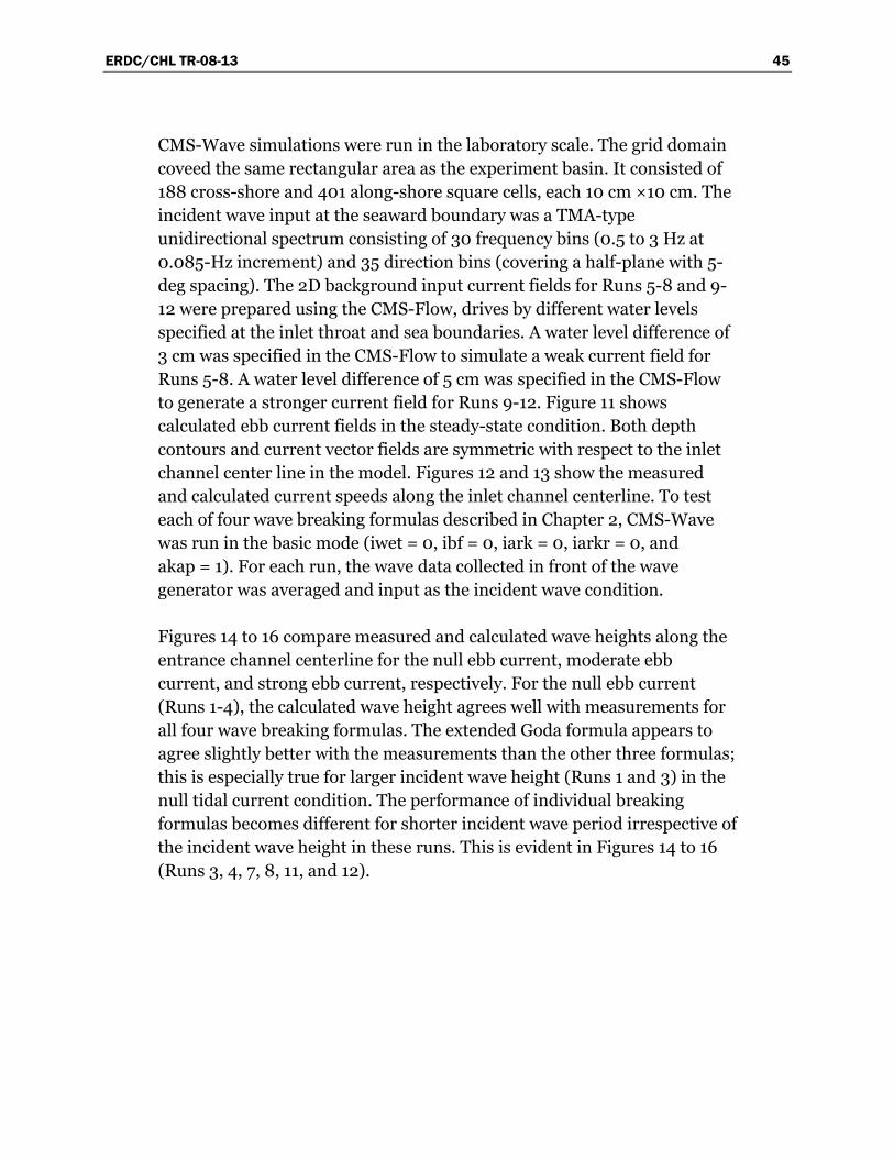
ERDC/CHL TR-08-13 45
CMS-Wave simulations were run in the laboratory scale. The grid domain coveed the same rectangular area as the experiment basin. It consisted of 188 cross-shore and 401 along-shore square cells, each 10 cm ×10 cm. The incident wave input at the seaward boundary was a TMA-type unidirectional spectrum consisting of 30 frequency bins (0.5 to 3 Hz at 0.085-Hz increment) and 35 direction bins (covering a half-plane with 5-deg spacing). The 2D background input current fields for Runs 5-8 and 9-12 were prepared using the CMS-Flow, drives by different water levels specified at the inlet throat and sea boundaries. A water level difference of 3 cm was specified in the CMS-Flow to simulate a weak current field for Runs 5-8. A water level difference of 5 cm was specified in the CMS-Flow to generate a stronger current field for Runs 9-12. Figure 11 shows calculated ebb current fields in the steady-state condition. Both depth contours and current vector fields are symmetric with respect to the inlet channel center line in the model. Figures 12 and 13 show the measured and calculated current speeds along the inlet channel centerline. To test each of four wave breaking formulas described in Chapter 2, CMS-Wave was run in the basic mode (iwet = 0, ibf = 0, iark = 0, iarkr = 0, and akap = 1). For each run, the wave data collected in front of the wave generator was averaged and input as the incident wave condition.
Figures 14 to 16 compare measured and calculated wave heights along the entrance channel centerline for the null ebb current, moderate ebb current, and strong ebb current, respectively. For the null ebb current (Runs 1-4), the calculated wave height agrees well with measurements for all four wave breaking formulas. The extended Goda formula appears to agree slightly better with the measurements than the other three formulas; this is especially true for larger incident wave height (Runs 1 and 3) in the null tidal current condition. The performance of individual breaking formulas becomes different for shorter incident wave period irrespective of the incident wave height in these runs. This is evident in Figures 14 to 16 (Runs 3, 4, 7, 8, 11, and 12).
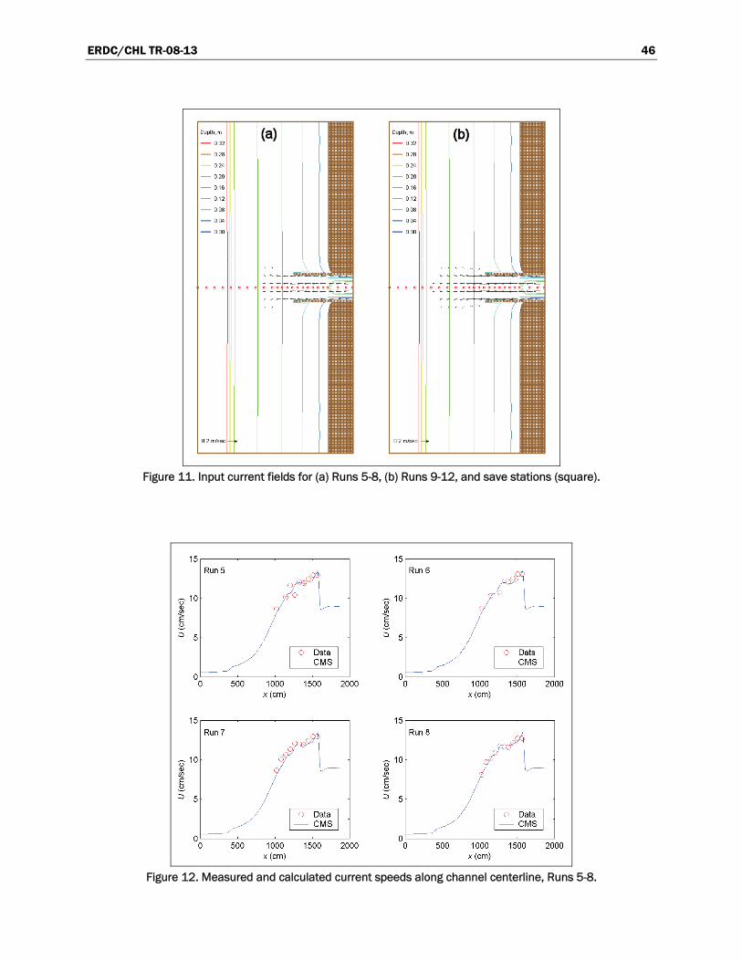
ERDC/CHL TR-08-13 46
Figure 11. Input current fields for (a) Runs 5-8, (b) Runs 9-12, and save stations (square).
Figure 12. Measured and calculated current speeds along channel centerline, Runs 5-8.
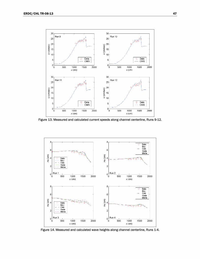
ERDC/CHL TR-08-13 47
Figure 13. Measured and calculated current speeds along channel centerline, Runs 9-12.
Figure 14. Measured and calculated wave heights along channel centerline, Runs 1-4.
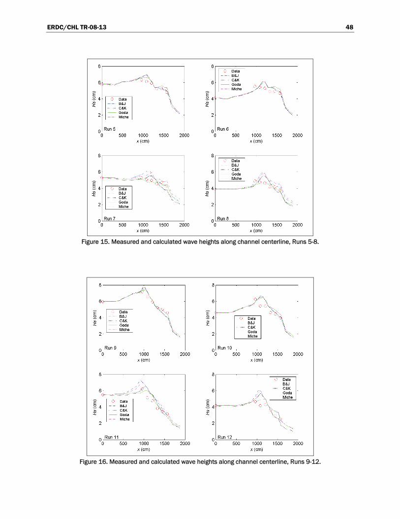
ERDC/CHL TR-08-13 48
Figure 15. Measured and calculated wave heights along channel centerline, Runs 5-8.
Figure 16. Measured and calculated wave heights along channel centerline, Runs 9-12.
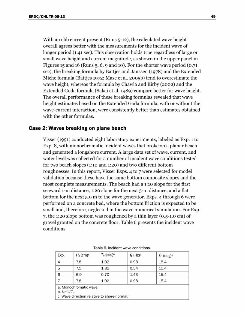
ERDC/CHL TR-08-13 49
With an ebb current present (Runs 5-12), the calculated wave height overall agrees better with the measurements for the incident wave of longer period (1.41 sec). This observation holds true regardless of large or small wave height and current magnitude, as shown in the upper panel in Figures 15 and 16 (Runs 5, 6, 9 and 10). For the shorter wave period (0.71 sec), the breaking formula by Battjes and Janssen (1978) and the Extended Miche formula (Battjes 1972; Mase et al. 2005b) tend to overestimate the wave height, whereas the formula by Chawla and Kirby (2002) and the Extended Goda formula (Sakai et al. 1989) compare better for wave height. The overall performance of these breaking formulas revealed that wave height estimates based on the Extended Goda formula, with or without the wave-current interaction, were consistently better than estimates obtained with the other formulas.
Case 2: Waves breaking on plane beach
Visser (1991) conducted eight laboratory experiments, labeled as Exp. 1 to Exp. 8, with monochromatic incident waves that broke on a planar beach and generated a longshore current. A large data set of wave, current, and water level was collected for a number of incident wave conditions tested for two beach slopes (1:10 and 1:20) and two different bottom roughnesses. In this report, Visser Exps. 4 to 7 were selected for model validation because these have the same bottom composite slopes and the most complete measurements. The beach had a 1:10 slope for the first seaward 1-m distance, 1:20 slope for the next 5-m distance, and a flat bottom for the next 5.9 m to the wave generator. Exps. 4 through 6 were performed on a concrete bed, where the bottom friction is expected to be small and, therefore, neglected in the wave numerical simulation. For Exp. 7, the 1:20 slope bottom was roughened by a thin layer (0.5-1.0 cm) of gravel grouted on the concrete floor. Table 6 presents the incident wave conditions.
Table 6. Incident wave conditions.
Exp. Hs (cm)a Tp (sec)a fp (Hz)b θ (deg)c 4 7.8 1.02 0.98 15.4 5 7.1 1.85 0.54 15.4 6 6.9 0.70 1.43 15.4 7 7.8 1.02 0.98 15.4 a. Monochromatic wave. b. fp=1/Tp. c. Wave direction relative to shore-normal.
ERDC/CHL TR-08-13 50
CMS-Wave was run at the laboratory scale. The model grid consisted of 90
cross-shore and 243 alongshore square cells, each 10 cm × 10 cm, to cover
the entire basin in these experiments. The spectral transformation was
computed in CMS-Wave on 11 frequency bins (covering the range of
+/- 0.05 Hz of the incident monochromatic wave frequency at 0.01-Hz
increment) and 35 direction bins (covering a half-plane with 5-deg
spacing). The incident monochromatic, unidirectional wave spectrum was
specified in a single frequency and direction bin at the seaward boundary.
The input current and water level fields were interpolated across shore and
averaged alongshore from the data. For Exp. 7 with the gravel floor, a
constant bottom friction coefficient cf of 0.01 was specified in CMS-Wave
and was found to produce good wave estimates.
Figure 17 shows an example of input current and water level fields to CMS-
Wave for the Exp. 4. Figure 18 compares the measured and calculated
across shore wave heights for Exp. 4 through 7. The calculated wave height
agrees well with the measurements for four different depth-limiting
breaking formulas implemented in CMS-Wave.
Case 3: Wave runup on impermeable uniform slope
Wave runup on a uniform slope calculated by CMS-Wave was compared to two laboratory experiments, one experiment conducted by Ahrens and Titus (1981) the other by Mase and Iwagaki (1984). Incident random waves were generated in both experiments in a wave flume consisting of a flat bottom connected to a slope. The experiments by Ahrens and Titus included 275 wave conditions (Ahrens and Heimbaugh 1988), with the significant wave heights ranging from 4 to 20 cm and spectral peak periods from 1.1 to 4.5 sec, on six different uniform slopes at 1:1, 2:3, 1:2, 2:5, 1:3, and 1:4. The experiments by Mase and Iwagaki tested 120 wave conditions (Mase 1989), with significant wave heights ranging from 2.7 to 11 cm and spectral peak periods from 0.8 to 2.5 sec, on four uniform slopes at 1:5, 1:10, 1:20, and 1:30.
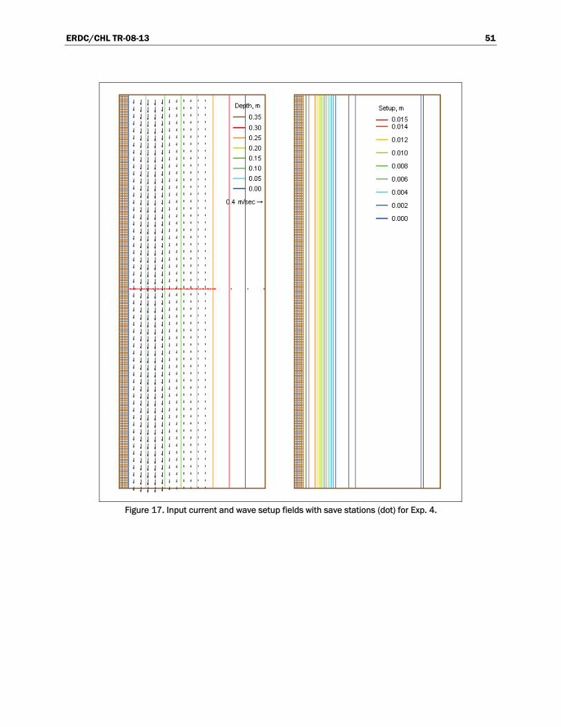
ERDC/CHL TR-08-13 51
Figure 17. Input current and wave setup fields with save stations (dot) for Exp. 4.
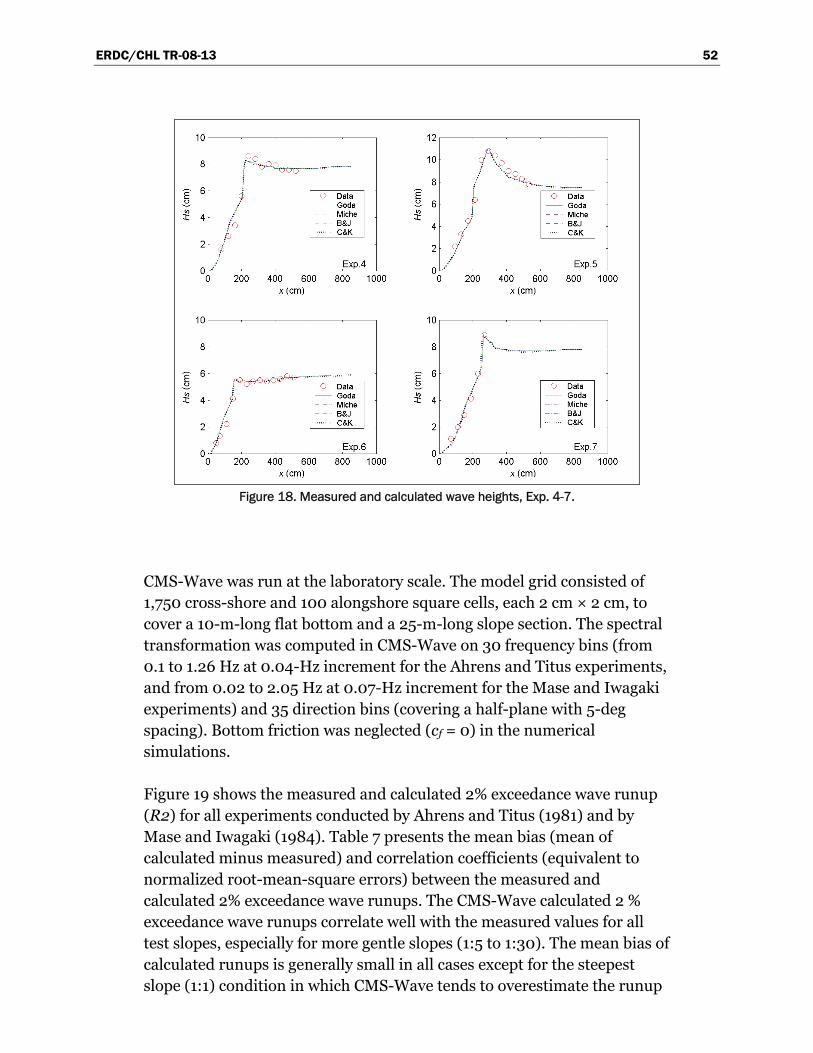
ERDC/CHL TR-08-13 52
Figure 18. Measured and calculated wave heights, Exp. 4-7.
CMS-Wave was run at the laboratory scale. The model grid consisted of 1,750 cross-shore and 100 alongshore square cells, each 2 cm × 2 cm, to cover a 10-m-long flat bottom and a 25-m-long slope section. The spectral transformation was computed in CMS-Wave on 30 frequency bins (from 0.1 to 1.26 Hz at 0.04-Hz increment for the Ahrens and Titus experiments, and from 0.02 to 2.05 Hz at 0.07-Hz increment for the Mase and Iwagaki experiments) and 35 direction bins (covering a half-plane with 5-deg spacing). Bottom friction was neglected (cf = 0) in the numerical simulations.
Figure 19 shows the measured and calculated 2% exceedance wave runup (R2) for all experiments conducted by Ahrens and Titus (1981) and by Mase and Iwagaki (1984). Table 7 presents the mean bias (mean of calculated minus measured) and correlation coefficients (equivalent to normalized root-mean-square errors) between the measured and calculated 2% exceedance wave runups. The CMS-Wave calculated 2 % exceedance wave runups correlate well with the measured values for all test slopes, especially for more gentle slopes (1:5 to 1:30). The mean bias of calculated runups is generally small in all cases except for the steepest slope (1:1) condition in which CMS-Wave tends to overestimate the runup
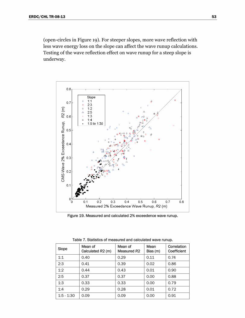
ERDC/CHL TR-08-13 53
(open-circles in Figure 19). For steeper slopes, more wave reflection with less wave energy loss on the slope can affect the wave runup calculations. Testing of the wave reflection effect on wave runup for a steep slope is underway.
Figure 19. Measured and calculated 2% exceedence wave runup.
Table 7. Statistics of measured and calculated wave runup.
Slope Mean of Calculated R2 (m)
Mean of Measured R2
Mean Bias (m)
Correlation Coefficient
1:1 0.40 0.29 0.11 0.74 2:3 0.41 0.39 0.02 0.86 1:2 0.44 0.43 0.01 0.90 2:5 0.37 0.37 0.00 0.88 1:3 0.33 0.33 0.00 0.79 1:4 0.29 0.28 0.01 0.72 1:5 - 1:30 0.09 0.09 0.00 0.91
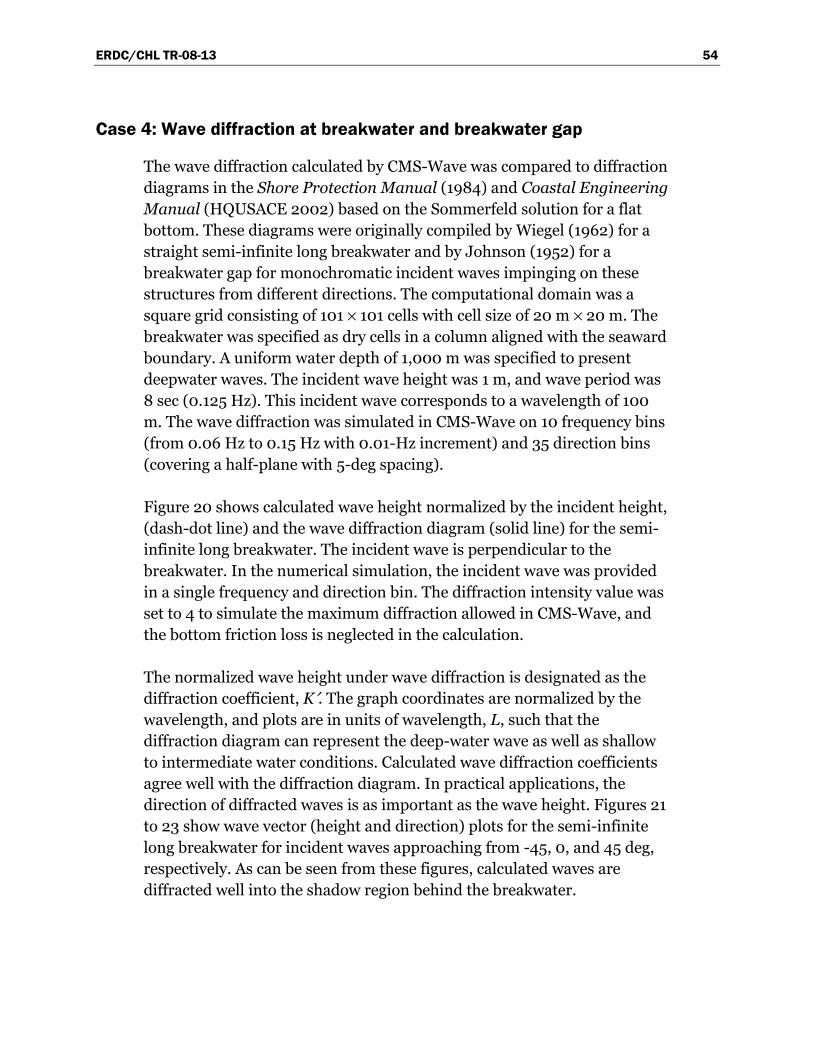
ERDC/CHL TR-08-13 54
Case 4: Wave diffraction at breakwater and breakwater gap
The wave diffraction calculated by CMS-Wave was compared to diffraction diagrams in the Shore Protection Manual (1984) and Coastal Engineering Manual (HQUSACE 2002) based on the Sommerfeld solution for a flat bottom. These diagrams were originally compiled by Wiegel (1962) for a straight semi-infinite long breakwater and by Johnson (1952) for a breakwater gap for monochromatic incident waves impinging on these structures from different directions. The computational domain was a square grid consisting of 101 × 101 cells with cell size of 20 m × 20 m. The breakwater was specified as dry cells in a column aligned with the seaward boundary. A uniform water depth of 1,000 m was specified to present deepwater waves. The incident wave height was 1 m, and wave period was 8 sec (0.125 Hz). This incident wave corresponds to a wavelength of 100 m. The wave diffraction was simulated in CMS-Wave on 10 frequency bins (from 0.06 Hz to 0.15 Hz with 0.01-Hz increment) and 35 direction bins (covering a half-plane with 5-deg spacing).
Figure 20 shows calculated wave height normalized by the incident height, (dash-dot line) and the wave diffraction diagram (solid line) for the semi-infinite long breakwater. The incident wave is perpendicular to the breakwater. In the numerical simulation, the incident wave was provided in a single frequency and direction bin. The diffraction intensity value was set to 4 to simulate the maximum diffraction allowed in CMS-Wave, and the bottom friction loss is neglected in the calculation.
The normalized wave height under wave diffraction is designated as the diffraction coefficient, K′. The graph coordinates are normalized by the wavelength, and plots are in units of wavelength, L, such that the diffraction diagram can represent the deep-water wave as well as shallow to intermediate water conditions. Calculated wave diffraction coefficients agree well with the diffraction diagram. In practical applications, the direction of diffracted waves is as important as the wave height. Figures 21 to 23 show wave vector (height and direction) plots for the semi-infinite long breakwater for incident waves approaching from -45, 0, and 45 deg, respectively. As can be seen from these figures, calculated waves are diffracted well into the shadow region behind the breakwater.
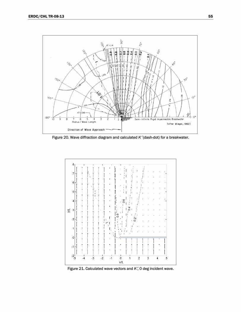
ERDC/CHL TR-08-13 55
Figure 20. Wave diffraction diagram and calculated K′ (dash-dot) for a breakwater.
Figure 21. Calculated wave vectors and K′, 0 deg incident wave.
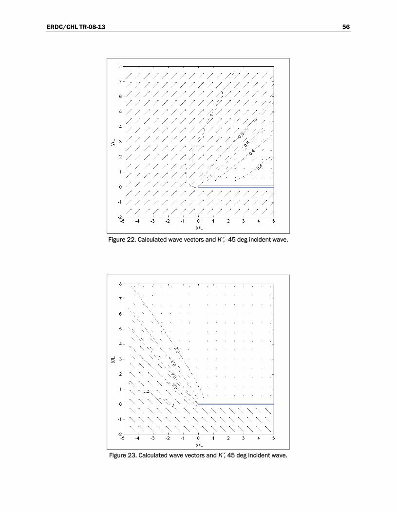
ERDC/CHL TR-08-13 56
Figure 22. Calculated wave vectors and K′, -45 deg incident wave.
Figure 23. Calculated wave vectors and K′, 45 deg incident wave.
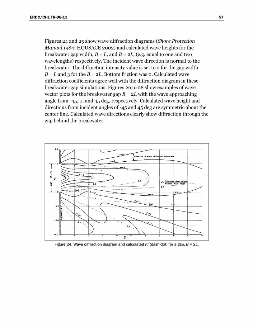
ERDC/CHL TR-08-13 57
Figures 24 and 25 show wave diffraction diagrams (Shore Protection Manual 1984; HQUSACE 2002) and calculated wave heights for the breakwater gap width, B = L, and B = 2L, (e.g. equal to one and two wavelengths) respectively. The incident wave direction is normal to the breakwater. The diffraction intensity value is set to 2 for the gap width B = L and 3 for the B = 2L. Bottom friction was 0. Calculated wave diffraction coefficients agree well with the diffraction diagram in these breakwater gap simulations. Figures 26 to 28 show examples of wave vector plots for the breakwater gap B = 2L with the wave approaching angle from -45, 0, and 45 deg, respectively. Calculated wave height and directions from incident angles of -45 and 45 deg are symmetric about the center line. Calculated wave directions clearly show diffraction through the gap behind the breakwater.
Figure 24. Wave diffraction diagram and calculated K′ (dash-dot) for a gap, B = 2L.
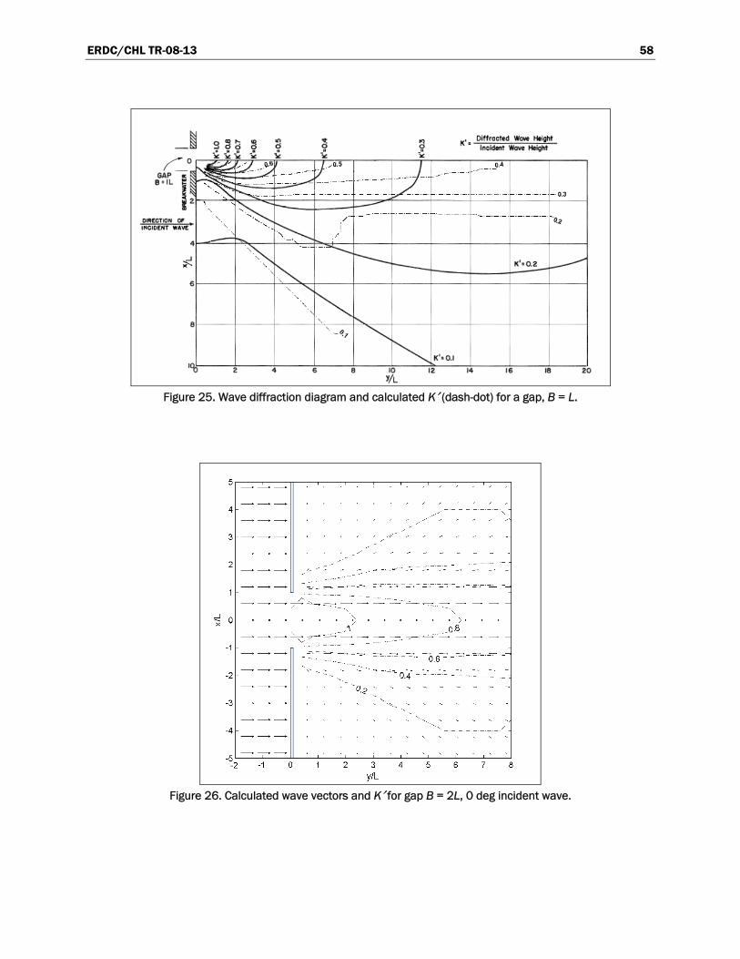
ERDC/CHL TR-08-13 58
Figure 25. Wave diffraction diagram and calculated K′ (dash-dot) for a gap, B = L.
Figure 26. Calculated wave vectors and K′ for gap B = 2L, 0 deg incident wave.
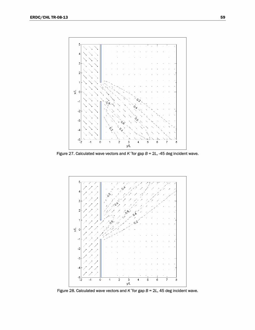
ERDC/CHL TR-08-13 59
Figure 27. Calculated wave vectors and K′ for gap B = 2L, -45 deg incident wave.
Figure 28. Calculated wave vectors and K′ for gap B = 2L, 45 deg incident wave.
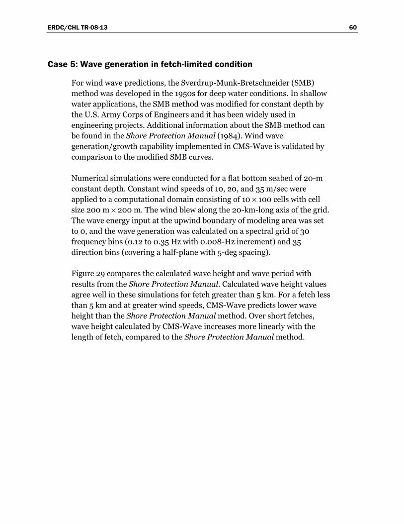
ERDC/CHL TR-08-13 60
Case 5: Wave generation in fetch-limited condition
For wind wave predictions, the Sverdrup-Munk-Bretschneider (SMB) method was developed in the 1950s for deep water conditions. In shallow water applications, the SMB method was modified for constant depth by the U.S. Army Corps of Engineers and it has been widely used in engineering projects. Additional information about the SMB method can be found in the Shore Protection Manual (1984). Wind wave generation/growth capability implemented in CMS-Wave is validated by comparison to the modified SMB curves.
Numerical simulations were conducted for a flat bottom seabed of 20-m constant depth. Constant wind speeds of 10, 20, and 35 m/sec were applied to a computational domain consisting of 10 × 100 cells with cell size 200 m × 200 m. The wind blew along the 20-km-long axis of the grid. The wave energy input at the upwind boundary of modeling area was set to 0, and the wave generation was calculated on a spectral grid of 30 frequency bins (0.12 to 0.35 Hz with 0.008-Hz increment) and 35 direction bins (covering a half-plane with 5-deg spacing).
Figure 29 compares the calculated wave height and wave period with results from the Shore Protection Manual. Calculated wave height values agree well in these simulations for fetch greater than 5 km. For a fetch less than 5 km and at greater wind speeds, CMS-Wave predicts lower wave height than the Shore Protection Manual method. Over short fetches, wave height calculated by CMS-Wave increases more linearly with the length of fetch, compared to the Shore Protection Manual method.
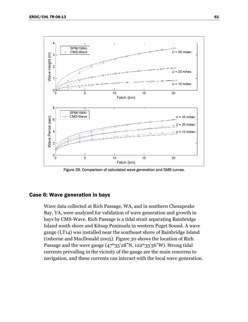
ERDC/CHL TR-08-13 61
Figure 29. Comparison of calculated wave generation and SMB curves.
Case 6: Wave generation in bays
Wave data collected at Rich Passage, WA, and in southern Chesapeake Bay, VA, were analyzed for validation of wave generation and growth in bays by CMS-Wave. Rich Passage is a tidal strait separating Bainbridge Island south shore and Kitsap Peninsula in western Puget Sound. A wave gauge (LT14) was installed near the southeast shore of Bainbridge Island (Osborne and MacDonald 2005). Figure 30 shows the location of Rich Passage and the wave gauge (47º35’28”N, 122º33’56”W). Strong tidal currents prevailing in the vicinity of the gauge are the main concerns to navigation, and these currents can interact with the local wave generation.
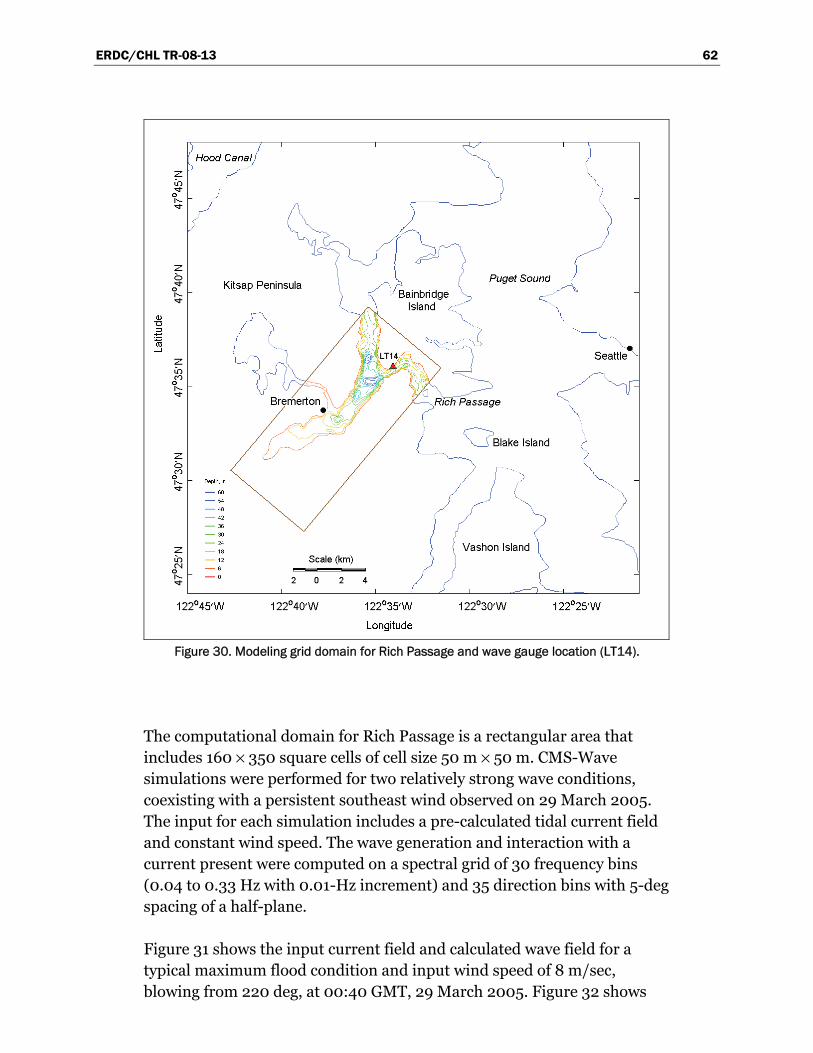
ERDC/CHL TR-08-13 62
Figure 30. Modeling grid domain for Rich Passage and wave gauge location (LT14).
The computational domain for Rich Passage is a rectangular area that includes 160 × 350 square cells of cell size 50 m × 50 m. CMS-Wave simulations were performed for two relatively strong wave conditions, coexisting with a persistent southeast wind observed on 29 March 2005. The input for each simulation includes a pre-calculated tidal current field and constant wind speed. The wave generation and interaction with a current present were computed on a spectral grid of 30 frequency bins (0.04 to 0.33 Hz with 0.01-Hz increment) and 35 direction bins with 5-deg spacing of a half-plane.
Figure 31 shows the input current field and calculated wave field for a typical maximum flood condition and input wind speed of 8 m/sec, blowing from 220 deg, at 00:40 GMT, 29 March 2005. Figure 32 shows
ERDC/CHL TR-08-13 63
the input current field and calculated wave field for a strong ebb condition and wind speed of 11 m/sec, blowing from 220 deg, at 19:20 GMT of the same day. Table 8 presents the measured and calculated wave heights at the wave gauge location of LT14. In both simulations, the calculated wave height is in good agreement with the measurements.
Figure 31. (a) Input current, and (b) calculated wave fields at 00:40 GMT, 29 March 2005.
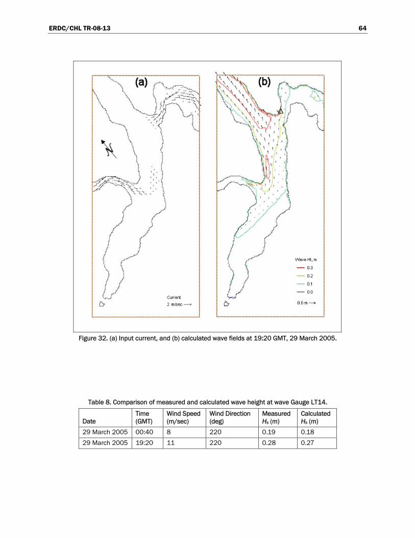
ERDC/CHL TR-08-13 64
Figure 32. (a) Input current, and (b) calculated wave fields at 19:20 GMT, 29 March 2005.
Table 8. Comparison of measured and calculated wave height at wave Gauge LT14.
Date Time (GMT)
Wind Speed (m/sec)
Wind Direction (deg)
Measured Hs (m)
Calculated Hs (m)
29 March 2005 00:40 8 220 0.19 0.18 29 March 2005 19:20 11 220 0.28 0.27
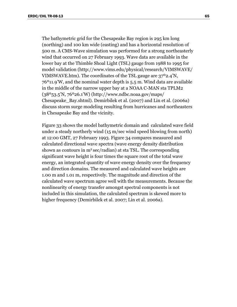
ERDC/CHL TR-08-13 65
The bathymetric grid for the Chesapeake Bay region is 295 km long (northing) and 100 km wide (easting) and has a horizontal resolution of 500 m. A CMS-Wave simulation was performed for a strong northeasterly wind that occurred on 27 February 1993. Wave data are available in the lower bay at the Thimble Shoal Light (TSL) gauge from 1988 to 1995 for model validation (http://www.vims.edu/physical/research/ VIMSWAVE/
VIMSWAVE.htm). The coordinates of the TSL gauge are 37º2.4’N, 76º11.9’W, and the nominal water depth is 5.5 m. Wind data are available in the middle of the narrow upper bay at a NOAA C-MAN sta TPLM2 (38º53.5’N, 76º26.1’W) (http://www.ndbc.noaa.gov/maps/ Chesapeake_Bay.shtml). Demirbilek et al. (2007) and Lin et al. (2006a) discuss storm surge modeling resulting from hurricanes and northeasters in Chesapeake Bay and the vicinity.
Figure 33 shows the model bathymetric domain and calculated wave field under a steady northerly wind (15 m/sec wind speed blowing from north) at 12:00 GMT, 27 February 1993. Figure 34 compares measured and calculated directional wave spectra (wave energy density distribution shown as contours in m2 sec/radian) at sta TSL. The corresponding significant wave height is four times the square root of the total wave energy, an integrated quantity of wave energy density over the frequency and direction domains. The measured and calculated wave heights are 1.00 m and 1.01 m, respectively. The magnitude and direction of the calculated wave spectrum agree well with the measurements. Because the nonlinearity of energy transfer amongst spectral components is not included in this simulation, the calculated spectrum is skewed more to higher frequency (Demirbilek et al. 2007; Lin et al. 2006a).
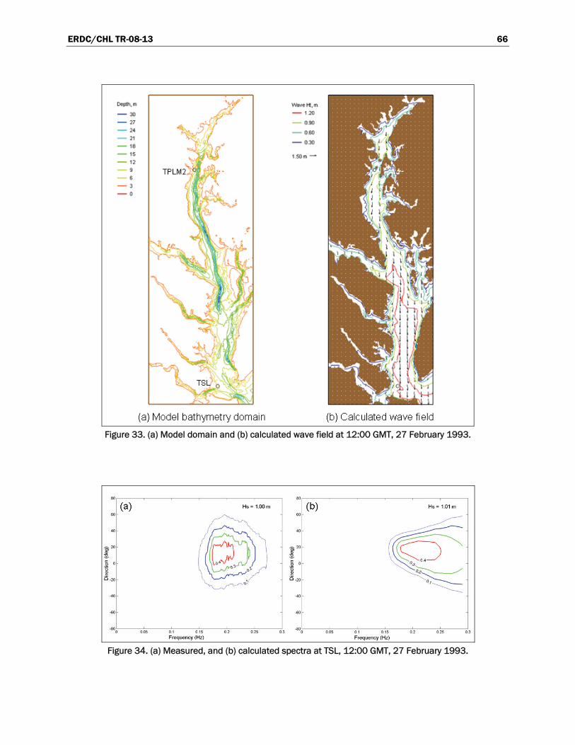
ERDC/CHL TR-08-13 66
Figure 33. (a) Model domain and (b) calculated wave field at 12:00 GMT, 27 February 1993.
Figure 34. (a) Measured, and (b) calculated spectra at TSL, 12:00 GMT, 27 February 1993.
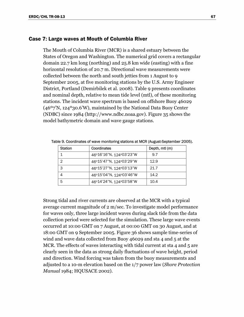
ERDC/CHL TR-08-13 67
Case 7: Large waves at Mouth of Columbia River
The Mouth of Columbia River (MCR) is a shared estuary between the States of Oregon and Washington. The numerical grid covers a rectangular domain 22.7 km long (northing) and 25.8 km wide (easting) with a fine horizontal resolution of 20.7 m. Directional wave measurements were collected between the north and south jetties from 1 August to 9 September 2005, at five monitoring stations by the U.S. Army Engineer District, Portland (Demirbilek et al. 2008). Table 9 presents coordinates and nominal depth, relative to mean tide level (mtl), of these monitoring stations. The incident wave spectrum is based on offshore Buoy 46029 (46º7’N, 124º30.6’W), maintained by the National Data Buoy Center (NDBC) since 1984 (http://www.ndbc.noaa.gov). Figure 35 shows the model bathymetric domain and wave gauge stations.
Table 9. Coordinates of wave monitoring stations at MCR (August-September 2005).
Station Coordinates Depth, mtl (m) 1 46o16’16”N, 124o03’23”W 9.7
2 46o15’47”N, 124o03’29”W 12.9
3 46o15’27”N, 124o03’13”W 21.7
4 46o15’04”N, 124o03’46”W 14.2
5 46o14’24”N, 124o03’58”W 10.4
Strong tidal and river currents are observed at the MCR with a typical average current magnitude of 2 m/sec. To investigate model performance for waves only, three large incident waves during slack tide from the data collection period were selected for the simulation. These large wave events occurred at 10:00 GMT on 7 August, at 00:00 GMT on 30 August, and at 18:00 GMT on 9 September 2005. Figure 36 shows sample time-series of wind and wave data collected from Buoy 46029 and sta 4 and 5 at the MCR. The effects of waves interacting with tidal current at sta 4 and 5 are clearly seen in the data as strong daily fluctuations of wave height, period and direction. Wind forcing was taken from the buoy measurements and adjusted to a 10-m elevation based on the 1/7 power law (Shore Protection Manual 1984; HQUSACE 2002).
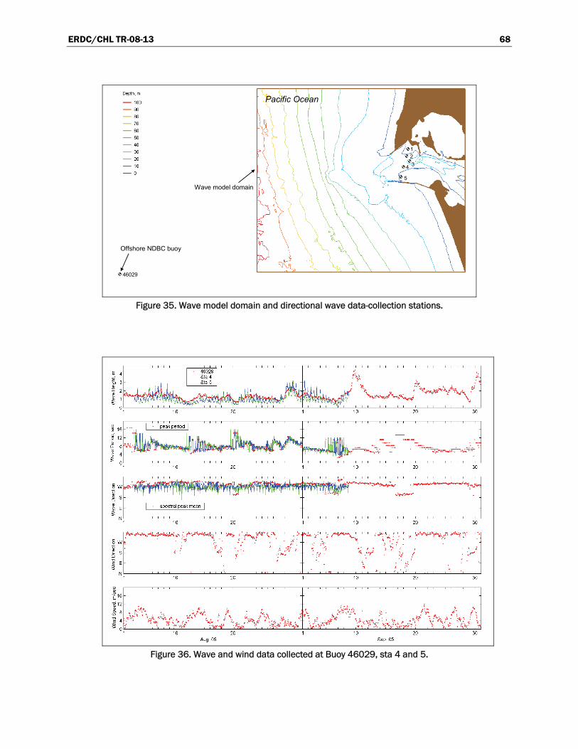
ERDC/CHL TR-08-13 68
46029
1234
5
Offshore NDBC buoy
Wave model domain
Pacific Ocean
46029
1234
5
Offshore NDBC buoy
Wave model domain
Pacific Ocean
Figure 35. Wave model domain and directional wave data-collection stations.
Figure 36. Wave and wind data collected at Buoy 46029, sta 4 and 5.
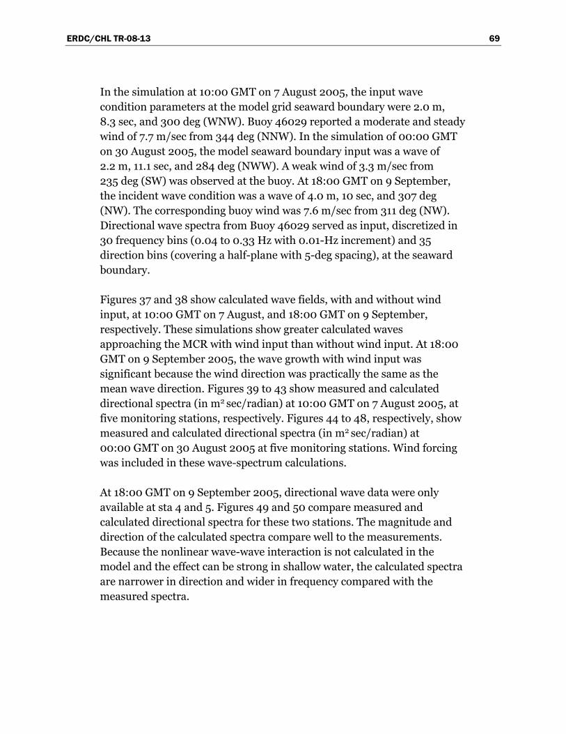
ERDC/CHL TR-08-13 69
In the simulation at 10:00 GMT on 7 August 2005, the input wave condition parameters at the model grid seaward boundary were 2.0 m, 8.3 sec, and 300 deg (WNW). Buoy 46029 reported a moderate and steady wind of 7.7 m/sec from 344 deg (NNW). In the simulation of 00:00 GMT on 30 August 2005, the model seaward boundary input was a wave of 2.2 m, 11.1 sec, and 284 deg (NWW). A weak wind of 3.3 m/sec from 235 deg (SW) was observed at the buoy. At 18:00 GMT on 9 September, the incident wave condition was a wave of 4.0 m, 10 sec, and 307 deg (NW). The corresponding buoy wind was 7.6 m/sec from 311 deg (NW). Directional wave spectra from Buoy 46029 served as input, discretized in 30 frequency bins (0.04 to 0.33 Hz with 0.01-Hz increment) and 35 direction bins (covering a half-plane with 5-deg spacing), at the seaward boundary.
Figures 37 and 38 show calculated wave fields, with and without wind input, at 10:00 GMT on 7 August, and 18:00 GMT on 9 September, respectively. These simulations show greater calculated waves approaching the MCR with wind input than without wind input. At 18:00 GMT on 9 September 2005, the wave growth with wind input was significant because the wind direction was practically the same as the mean wave direction. Figures 39 to 43 show measured and calculated directional spectra (in m2 sec/radian) at 10:00 GMT on 7 August 2005, at five monitoring stations, respectively. Figures 44 to 48, respectively, show measured and calculated directional spectra (in m2 sec/radian) at 00:00 GMT on 30 August 2005 at five monitoring stations. Wind forcing was included in these wave-spectrum calculations.
At 18:00 GMT on 9 September 2005, directional wave data were only available at sta 4 and 5. Figures 49 and 50 compare measured and calculated directional spectra for these two stations. The magnitude and direction of the calculated spectra compare well to the measurements. Because the nonlinear wave-wave interaction is not calculated in the model and the effect can be strong in shallow water, the calculated spectra are narrower in direction and wider in frequency compared with the measured spectra.
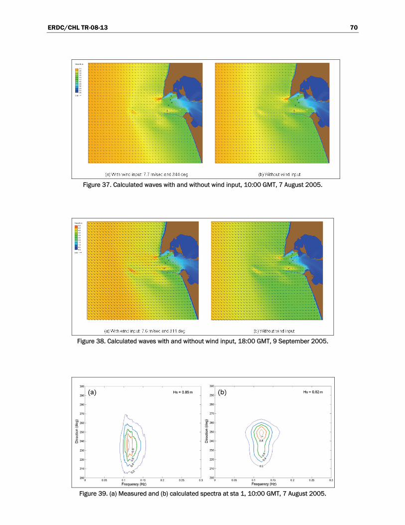
ERDC/CHL TR-08-13 70
Figure 37. Calculated waves with and without wind input, 10:00 GMT, 7 August 2005.
Figure 38. Calculated waves with and without wind input, 18:00 GMT, 9 September 2005.
Figure 39. (a) Measured and (b) calculated spectra at sta 1, 10:00 GMT, 7 August 2005.
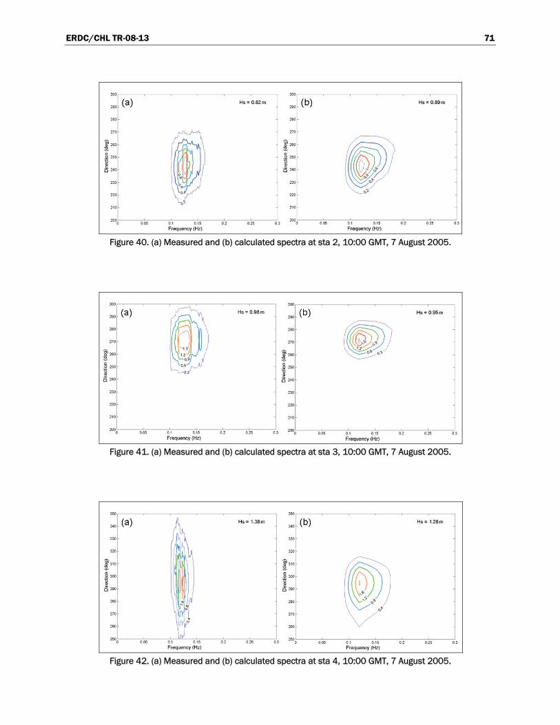
ERDC/CHL TR-08-13 71
Figure 40. (a) Measured and (b) calculated spectra at sta 2, 10:00 GMT, 7 August 2005.
Figure 41. (a) Measured and (b) calculated spectra at sta 3, 10:00 GMT, 7 August 2005.
Figure 42. (a) Measured and (b) calculated spectra at sta 4, 10:00 GMT, 7 August 2005.
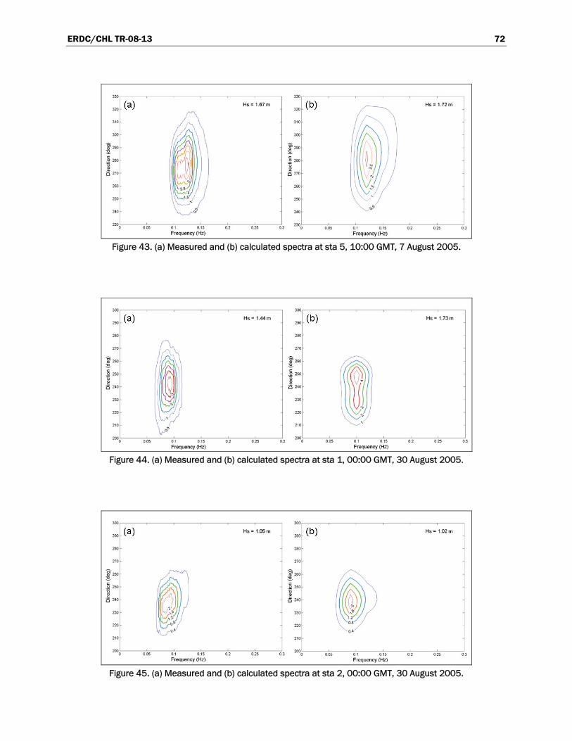
ERDC/CHL TR-08-13 72
Figure 43. (a) Measured and (b) calculated spectra at sta 5, 10:00 GMT, 7 August 2005.
Figure 44. (a) Measured and (b) calculated spectra at sta 1, 00:00 GMT, 30 August 2005.
Figure 45. (a) Measured and (b) calculated spectra at sta 2, 00:00 GMT, 30 August 2005.
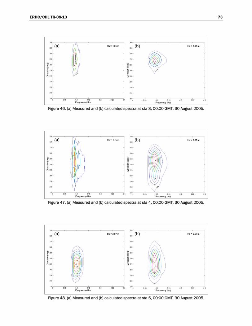
ERDC/CHL TR-08-13 73
Figure 46. (a) Measured and (b) calculated spectra at sta 3, 00:00 GMT, 30 August 2005.
Figure 47. (a) Measured and (b) calculated spectra at sta 4, 00:00 GMT, 30 August 2005.
Figure 48. (a) Measured and (b) calculated spectra at sta 5, 00:00 GMT, 30 August 2005.
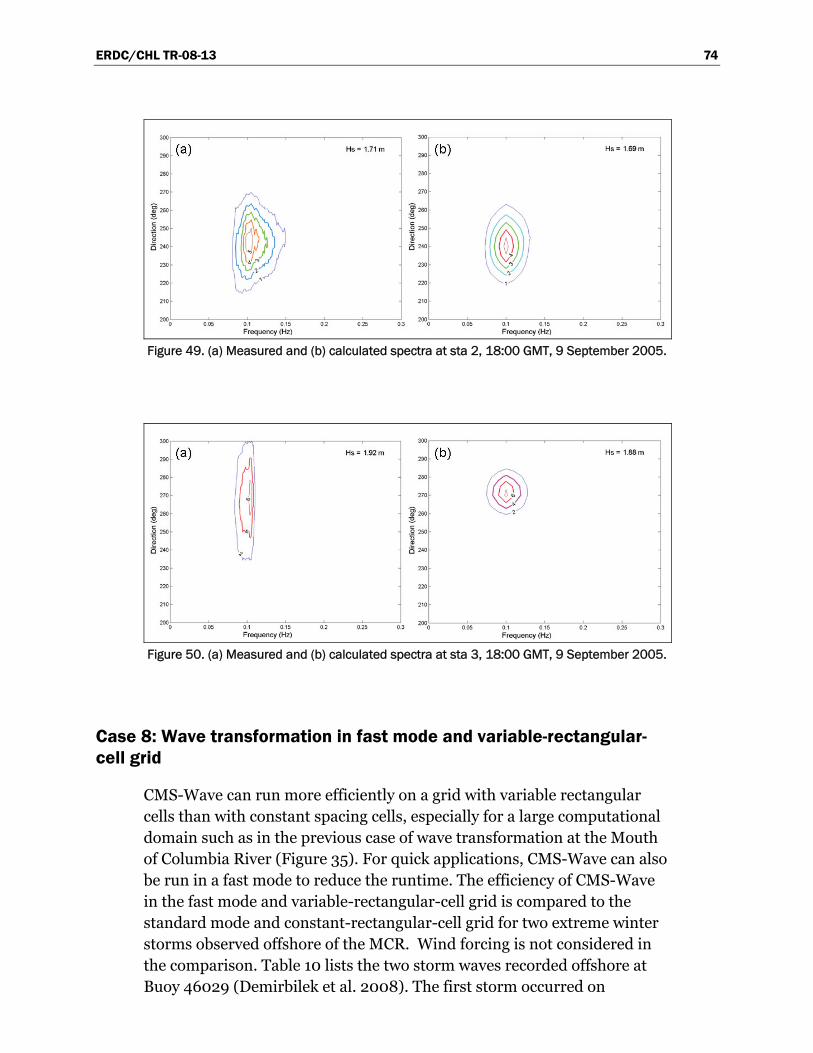
ERDC/CHL TR-08-13 74
Figure 49. (a) Measured and (b) calculated spectra at sta 2, 18:00 GMT, 9 September 2005.
Figure 50. (a) Measured and (b) calculated spectra at sta 3, 18:00 GMT, 9 September 2005.
Case 8: Wave transformation in fast mode and variable-rectangular-cell grid
CMS-Wave can run more efficiently on a grid with variable rectangular cells than with constant spacing cells, especially for a large computational domain such as in the previous case of wave transformation at the Mouth of Columbia River (Figure 35). For quick applications, CMS-Wave can also be run in a fast mode to reduce the runtime. The efficiency of CMS-Wave in the fast mode and variable-rectangular-cell grid is compared to the standard mode and constant-rectangular-cell grid for two extreme winter storms observed offshore of the MCR. Wind forcing is not considered in the comparison. Table 10 lists the two storm waves recorded offshore at Buoy 46029 (Demirbilek et al. 2008). The first storm occurred on
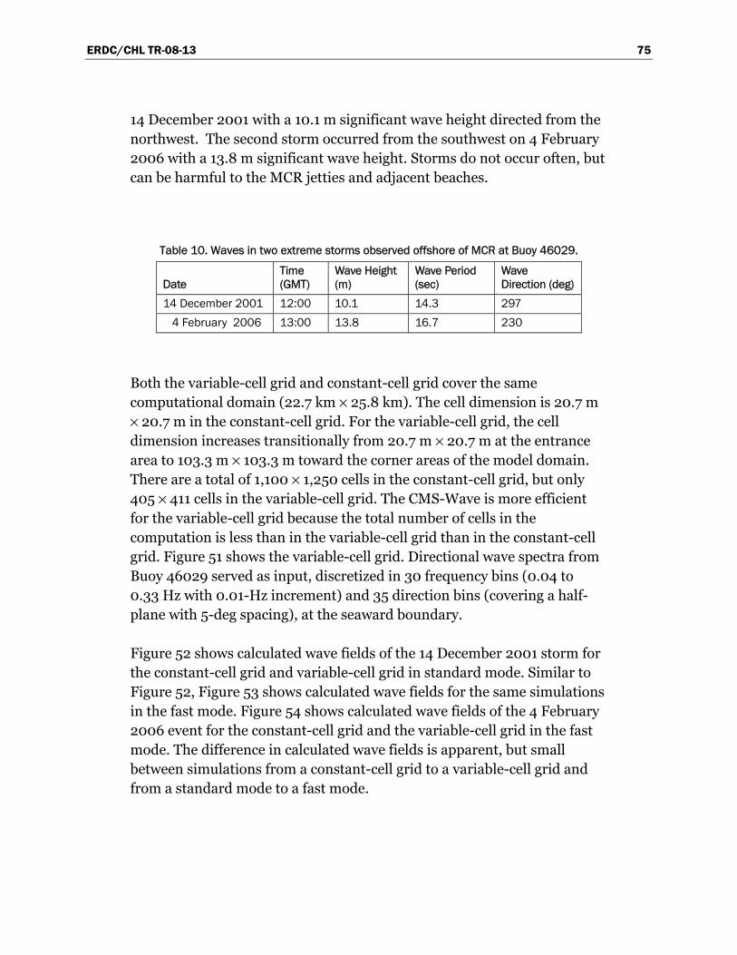
ERDC/CHL TR-08-13 75
14 December 2001 with a 10.1 m significant wave height directed from the northwest. The second storm occurred from the southwest on 4 February 2006 with a 13.8 m significant wave height. Storms do not occur often, but can be harmful to the MCR jetties and adjacent beaches.
Table 10. Waves in two extreme storms observed offshore of MCR at Buoy 46029.
Date Time (GMT)
Wave Height (m)
Wave Period (sec)
Wave Direction (deg)
14 December 2001 12:00 10.1 14.3 297 4 February 2006 13:00 13.8 16.7 230
Both the variable-cell grid and constant-cell grid cover the same computational domain (22.7 km × 25.8 km). The cell dimension is 20.7 m × 20.7 m in the constant-cell grid. For the variable-cell grid, the cell dimension increases transitionally from 20.7 m × 20.7 m at the entrance area to 103.3 m × 103.3 m toward the corner areas of the model domain. There are a total of 1,100 × 1,250 cells in the constant-cell grid, but only 405 × 411 cells in the variable-cell grid. The CMS-Wave is more efficient for the variable-cell grid because the total number of cells in the computation is less than in the variable-cell grid than in the constant-cell grid. Figure 51 shows the variable-cell grid. Directional wave spectra from Buoy 46029 served as input, discretized in 30 frequency bins (0.04 to 0.33 Hz with 0.01-Hz increment) and 35 direction bins (covering a half-plane with 5-deg spacing), at the seaward boundary.
Figure 52 shows calculated wave fields of the 14 December 2001 storm for the constant-cell grid and variable-cell grid in standard mode. Similar to Figure 52, Figure 53 shows calculated wave fields for the same simulations in the fast mode. Figure 54 shows calculated wave fields of the 4 February 2006 event for the constant-cell grid and the variable-cell grid in the fast mode. The difference in calculated wave fields is apparent, but small between simulations from a constant-cell grid to a variable-cell grid and from a standard mode to a fast mode.
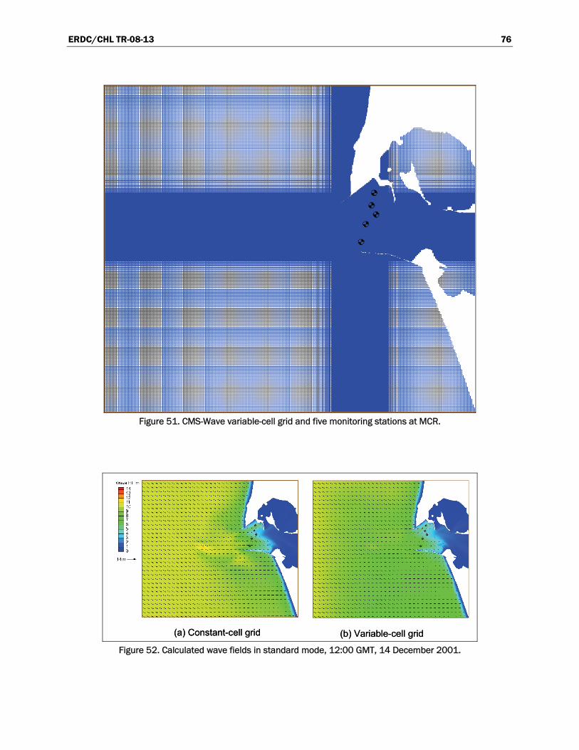
ERDC/CHL TR-08-13 76
Figure 51. CMS-Wave variable-cell grid and five monitoring stations at MCR.
(a) Constant-cell grid (b) Variable-cell grid(a) Constant-cell grid (b) Variable-cell grid Figure 52. Calculated wave fields in standard mode, 12:00 GMT, 14 December 2001.
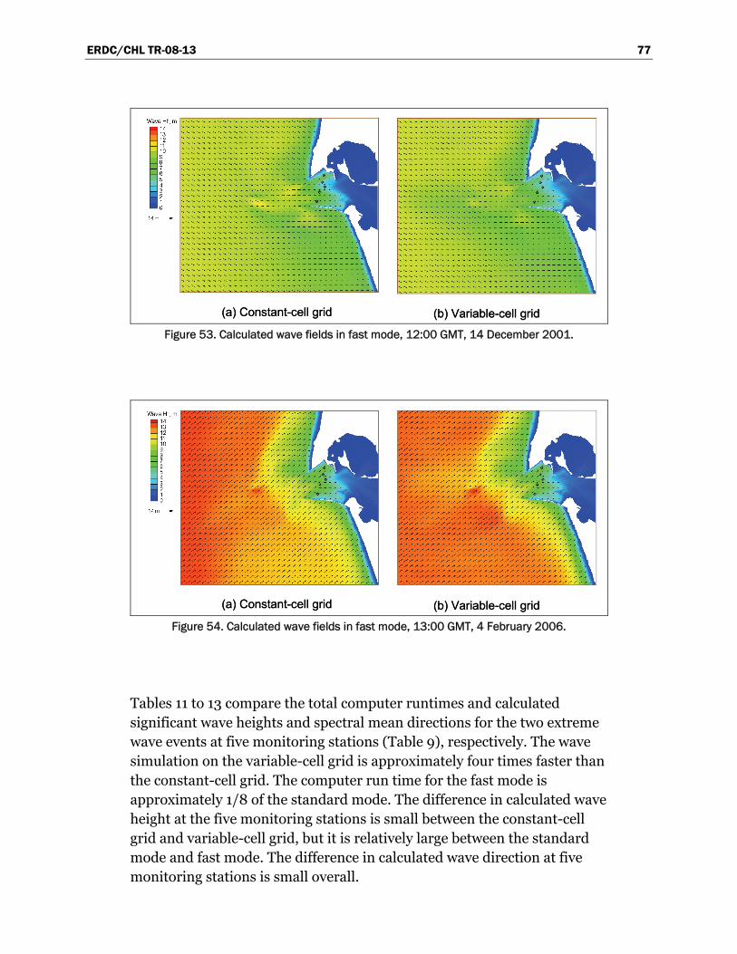
ERDC/CHL TR-08-13 77
(a) Constant-cell grid (b) Variable-cell grid(a) Constant-cell grid (b) Variable-cell grid Figure 53. Calculated wave fields in fast mode, 12:00 GMT, 14 December 2001.
(a) Constant-cell grid (b) Variable-cell grid(a) Constant-cell grid (b) Variable-cell grid Figure 54. Calculated wave fields in fast mode, 13:00 GMT, 4 February 2006.
Tables 11 to 13 compare the total computer runtimes and calculated significant wave heights and spectral mean directions for the two extreme wave events at five monitoring stations (Table 9), respectively. The wave simulation on the variable-cell grid is approximately four times faster than the constant-cell grid. The computer run time for the fast mode is approximately 1/8 of the standard mode. The difference in calculated wave height at the five monitoring stations is small between the constant-cell grid and variable-cell grid, but it is relatively large between the standard mode and fast mode. The difference in calculated wave direction at five monitoring stations is small overall.
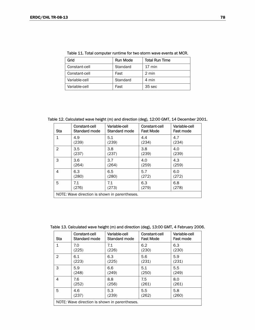
ERDC/CHL TR-08-13 78
Table 11. Total computer runtime for two storm wave events at MCR.
Grid Run Mode Total Run Time Constant-cell Standard 17 min Constant-cell Fast 2 min Variable-cell Standard 4 min Variable-cell Fast 35 sec
Table 12. Calculated wave height (m) and direction (deg), 12:00 GMT, 14 December 2001.
Sta Constant-cell Standard mode
Variable-cell Standard mode
Constant-cell Fast Mode
Variable-cell Fast mode
1 4.9 (239)
5.1 (239)
4.4 (234)
4.7 (234)
2 3.5 (237)
3.8 (237)
3.8 (239)
4.0 (239)
3 3.6 (264)
3.7 (264)
4.0 (259)
4.3 (259)
4 6.3 (280)
6.5 (280)
5.7 (272)
6.0 (272)
5 7.1 (276)
7.1 (273)
6.3 (279)
6.8 (278)
NOTE: Wave direction is shown in parentheses.
Table 13. Calculated wave height (m) and direction (deg), 13:00 GMT, 4 February 2006.
Sta Constant-cell Standard mode
Variable-cell Standard mode
Constant-cell Fast Mode
Variable-cell Fast mode
1 7.0 (225)
7.1 (226)
6.2 (230)
6.3 (230)
2 6.1 (223)
6.3 (225)
5.6 (231)
5.9 (231)
3 5.9 (248)
6.6 (249)
5.1 (250)
5.5 (249)
4 7.6 (252)
8.8 (256)
7.5 (261)
8.0 (261)
5 4.6 (237)
5.3 (239)
5.5 (262)
5.8 (260)
NOTE: Wave direction is shown in parentheses.
ERDC/CHL TR-08-13 79
Case 9: Wave transformation over complicated bathymetry with strong nearshore current
Laboratory experiments on wave transformation over a complicated bathymetry were conducted in the Research and Development Department of the Kansai Electric Power Co. Inc, Japan (Zheng et al. 2008). The physical model was built in a wave basin 20 m long and 38 m wide. The model to prototype scale was 1:125. Figure 55 shows the nearshore bathymetry and data-collection locations (circles). A snake-type wave maker generated incident wave spectra at the offshore boundary. Wave conditions included directional and unidirectional spectra. The input significant wave was 7.3 cm and 1.21 sec, simulating a 100-year return period. The directional spectrum was based on the Mitsuyasu distribution (Mitsuyasu and Honda 1982) with the spreading of direction in a standard deviation of 20 deg symmetric to the center angle.
Figure 56 displays measured directional and unidirectional wave height contours as well as the current induced by breaking waves. The wave-induced longshore current direction is from north to south in the physical model. The current can become strong at the concave shoreline (the maximum current speed reaches 0.25 m/sec in the model or equivalent to 2.7 m/sec in the prototype for unidirectional waves), where the incident waves converge and break toward the shore. The current outside the surf zone is overall weak (less than 0.05 m/sec) and opposite the wave propagation direction.
In this section, four depth-limited wave breaking criteria are examined with laboratory data.
Numerical simulations were carried out in the laboratory scale. The model grid domain is the same as the laboratory basin with the grid cell size of 0.2 m × 0.2 m. A standard JONSWAP spectrum was generated for the incident waves, consisting of 10 frequency bins and 36 direction bins. The current velocity in each cell was interpolated from the measurements. The variation of water level caused by wave setup was not considered in the simulations. Bottom friction was set to 0 in the model.
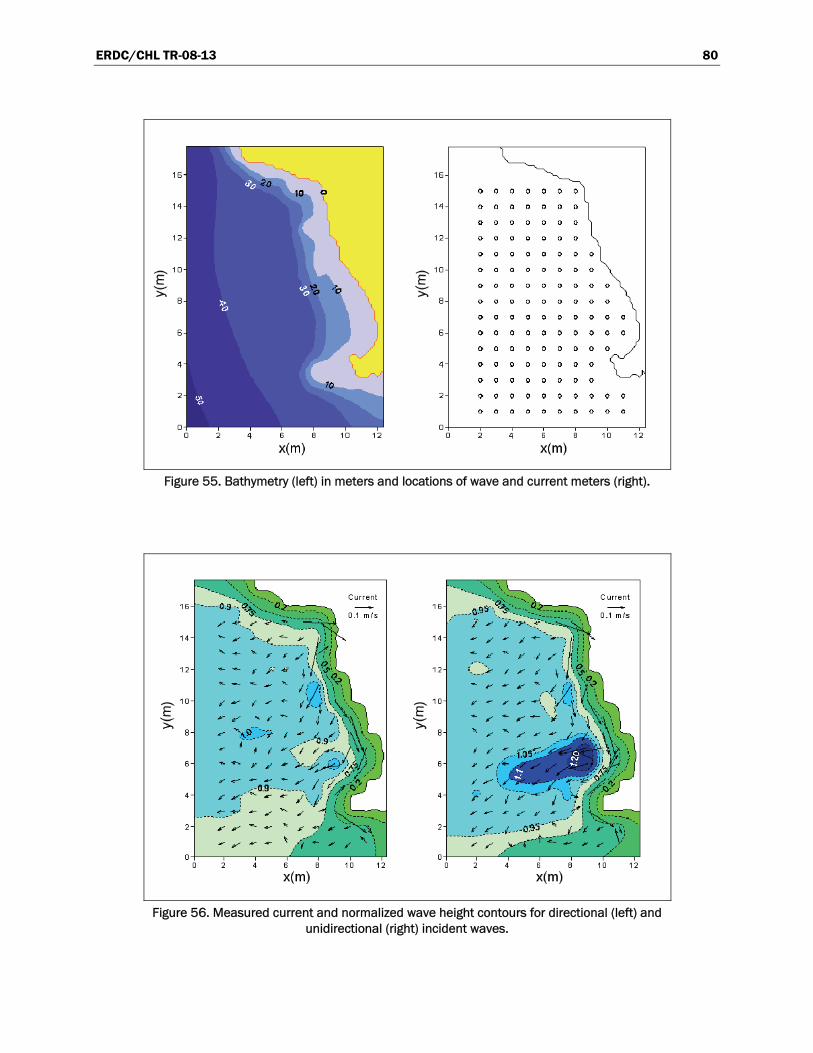
ERDC/CHL TR-08-13 80
Figure 55. Bathymetry (left) in meters and locations of wave and current meters (right).
Figure 56. Measured current and normalized wave height contours for directional (left) and
unidirectional (right) incident waves.

ERDC/CHL TR-08-13 81
Extended Miche formula
Figures 57 and 58 show calculated wave height contours for directional and unidirectional incident waves, with and without a current present using the Extended Miche breaking formula. The numerical result is more accurate with the background current included in the calculation.
Figure 57. Calculated wave height contours for directional incident waves without current
(left) and with current (right) by the Extended Miche formula with coefficient of 0.14.
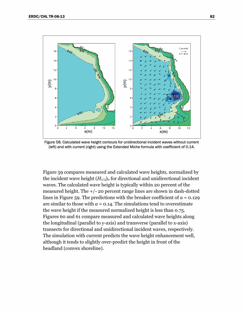
ERDC/CHL TR-08-13 82
Figure 58. Calculated wave height contours for unidirectional incident waves without current
(left) and with current (right) using the Extended Miche formula with coefficient of 0.14.
Figure 59 compares measured and calculated wave heights, normalized by the incident wave height (H1/3)0 for directional and unidirectional incident waves. The calculated wave height is typically within 20 percent of the measured height. The +/- 20 percent range lines are shown in dash-dotted lines in Figure 59. The predictions with the breaker coefficient of a = 0.129 are similar to those with a = 0.14. The simulations tend to overestimate the wave height if the measured normalized height is less than 0.75. Figures 60 and 61 compare measured and calculated wave heights along the longitudinal (parallel to y-axis) and transverse (parallel to x-axis) transects for directional and unidirectional incident waves, respectively. The simulation with current predicts the wave height enhancement well, although it tends to slightly over-predict the height in front of the headland (convex shoreline).
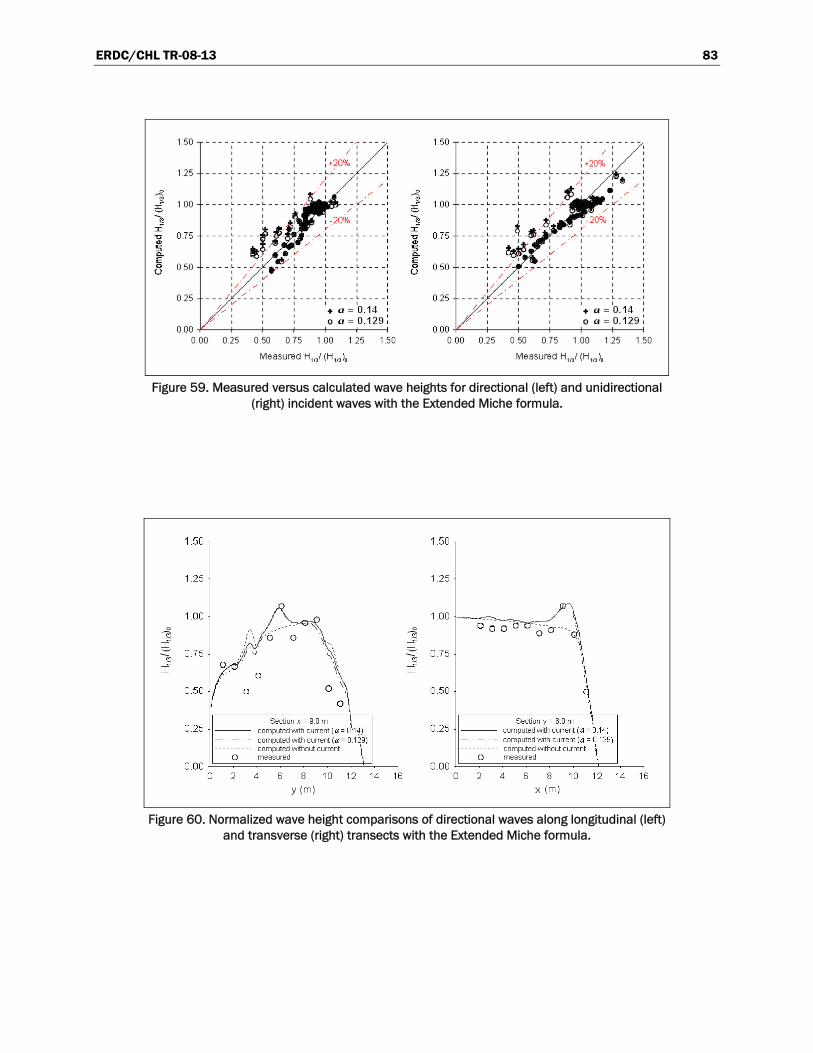
ERDC/CHL TR-08-13 83
Figure 59. Measured versus calculated wave heights for directional (left) and unidirectional
(right) incident waves with the Extended Miche formula.
Figure 60. Normalized wave height comparisons of directional waves along longitudinal (left)
and transverse (right) transects with the Extended Miche formula.
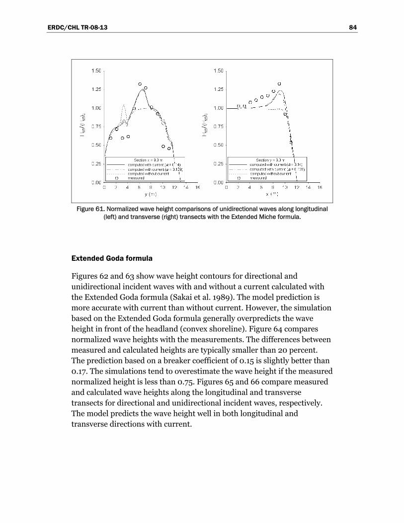
ERDC/CHL TR-08-13 84
Figure 61. Normalized wave height comparisons of unidirectional waves along longitudinal
(left) and transverse (right) transects with the Extended Miche formula.
Extended Goda formula
Figures 62 and 63 show wave height contours for directional and unidirectional incident waves with and without a current calculated with the Extended Goda formula (Sakai et al. 1989). The model prediction is more accurate with current than without current. However, the simulation based on the Extended Goda formula generally overpredicts the wave height in front of the headland (convex shoreline). Figure 64 compares normalized wave heights with the measurements. The differences between measured and calculated heights are typically smaller than 20 percent. The prediction based on a breaker coefficient of 0.15 is slightly better than 0.17. The simulations tend to overestimate the wave height if the measured normalized height is less than 0.75. Figures 65 and 66 compare measured and calculated wave heights along the longitudinal and transverse transects for directional and unidirectional incident waves, respectively. The model predicts the wave height well in both longitudinal and transverse directions with current.
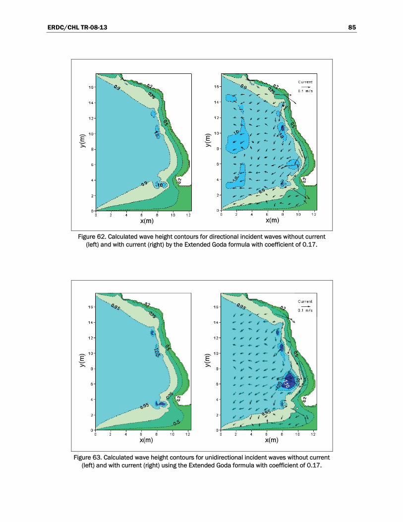
ERDC/CHL TR-08-13 85
Figure 62. Calculated wave height contours for directional incident waves without current
(left) and with current (right) by the Extended Goda formula with coefficient of 0.17.
Figure 63. Calculated wave height contours for unidirectional incident waves without current
(left) and with current (right) using the Extended Goda formula with coefficient of 0.17.
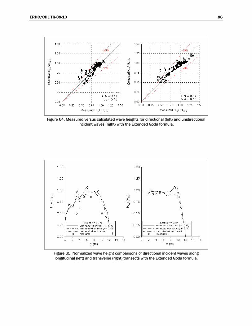
ERDC/CHL TR-08-13 86
Figure 64. Measured versus calculated wave heights for directional (left) and unidirectional
incident waves (right) with the Extended Goda formula.
Figure 65. Normalized wave height comparisons of directional incident waves along longitudinal (left) and transverse (right) transects with the Extended Goda formula.
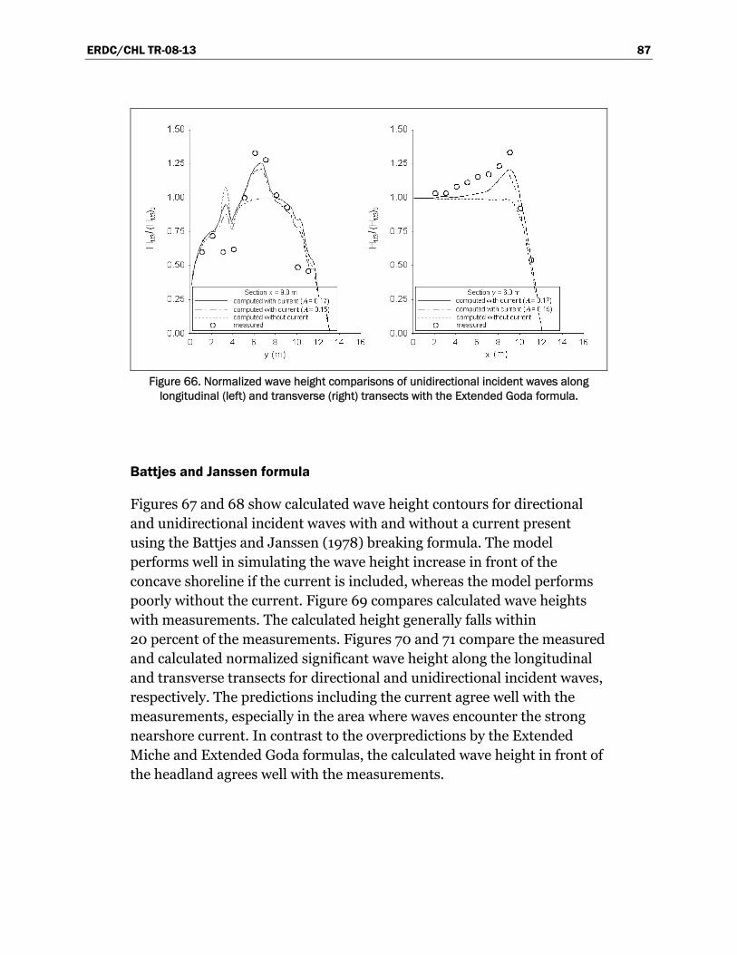
ERDC/CHL TR-08-13 87
Figure 66. Normalized wave height comparisons of unidirectional incident waves along
longitudinal (left) and transverse (right) transects with the Extended Goda formula.
Battjes and Janssen formula
Figures 67 and 68 show calculated wave height contours for directional and unidirectional incident waves with and without a current present using the Battjes and Janssen (1978) breaking formula. The model performs well in simulating the wave height increase in front of the concave shoreline if the current is included, whereas the model performs poorly without the current. Figure 69 compares calculated wave heights with measurements. The calculated height generally falls within 20 percent of the measurements. Figures 70 and 71 compare the measured and calculated normalized significant wave height along the longitudinal and transverse transects for directional and unidirectional incident waves, respectively. The predictions including the current agree well with the measurements, especially in the area where waves encounter the strong nearshore current. In contrast to the overpredictions by the Extended Miche and Extended Goda formulas, the calculated wave height in front of the headland agrees well with the measurements.
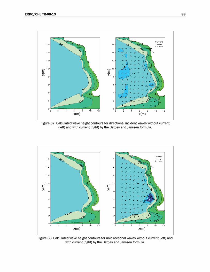
ERDC/CHL TR-08-13 88
Figure 67. Calculated wave height contours for directional incident waves without current
(left) and with current (right) by the Battjes and Janssen formula.
Figure 68. Calculated wave height contours for unidirectional waves without current (left) and
with current (right) by the Battjes and Janssen formula.
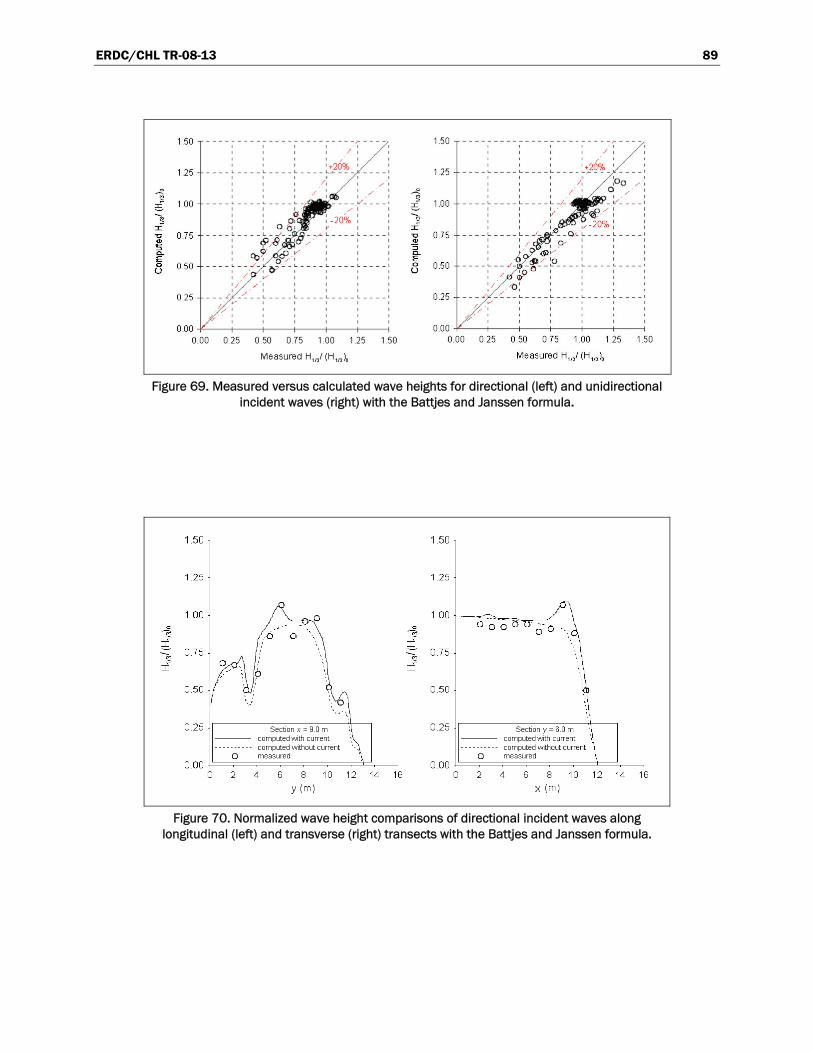
ERDC/CHL TR-08-13 89
Figure 69. Measured versus calculated wave heights for directional (left) and unidirectional
incident waves (right) with the Battjes and Janssen formula.
Figure 70. Normalized wave height comparisons of directional incident waves along
longitudinal (left) and transverse (right) transects with the Battjes and Janssen formula.
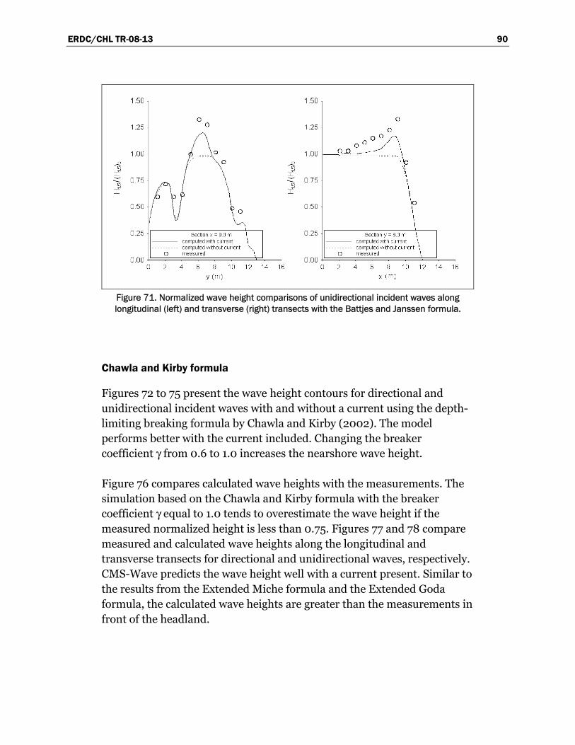
ERDC/CHL TR-08-13 90
Figure 71. Normalized wave height comparisons of unidirectional incident waves along longitudinal (left) and transverse (right) transects with the Battjes and Janssen formula.
Chawla and Kirby formula
Figures 72 to 75 present the wave height contours for directional and unidirectional incident waves with and without a current using the depth-limiting breaking formula by Chawla and Kirby (2002). The model performs better with the current included. Changing the breaker coefficient γ from 0.6 to 1.0 increases the nearshore wave height.
Figure 76 compares calculated wave heights with the measurements. The simulation based on the Chawla and Kirby formula with the breaker coefficient γ equal to 1.0 tends to overestimate the wave height if the measured normalized height is less than 0.75. Figures 77 and 78 compare measured and calculated wave heights along the longitudinal and transverse transects for directional and unidirectional waves, respectively. CMS-Wave predicts the wave height well with a current present. Similar to the results from the Extended Miche formula and the Extended Goda formula, the calculated wave heights are greater than the measurements in front of the headland.
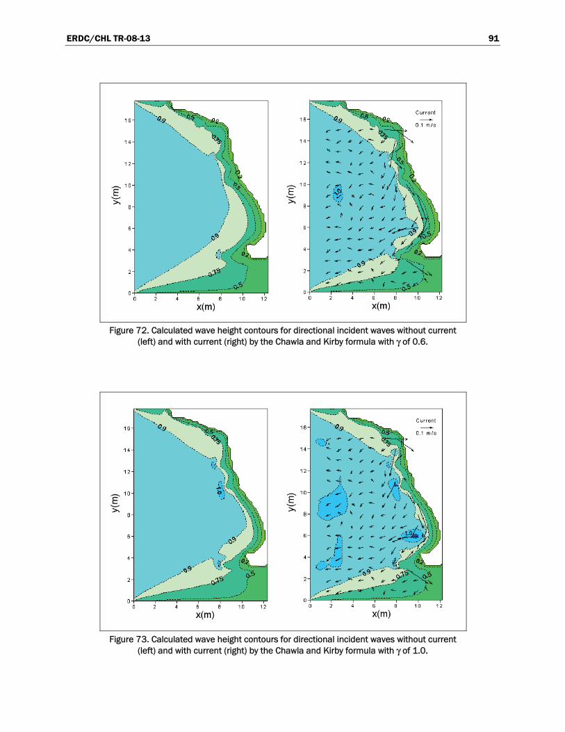
ERDC/CHL TR-08-13 91
Figure 72. Calculated wave height contours for directional incident waves without current
(left) and with current (right) by the Chawla and Kirby formula with γ of 0.6.
Figure 73. Calculated wave height contours for directional incident waves without current
(left) and with current (right) by the Chawla and Kirby formula with γ of 1.0.
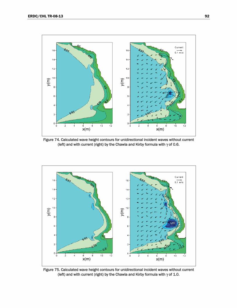
ERDC/CHL TR-08-13 92
Figure 74. Calculated wave height contours for unidirectional incident waves without current
(left) and with current (right) by the Chawla and Kirby formula with γ of 0.6.
Figure 75. Calculated wave height contours for unidirectional incident waves without current
(left) and with current (right) by the Chawla and Kirby formula with γ of 1.0.
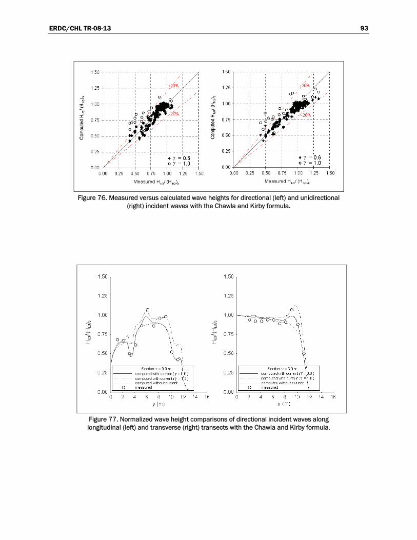
ERDC/CHL TR-08-13 93
Figure 76. Measured versus calculated wave heights for directional (left) and unidirectional
(right) incident waves with the Chawla and Kirby formula.
Figure 77. Normalized wave height comparisons of directional incident waves along longitudinal (left) and transverse (right) transects with the Chawla and Kirby formula.
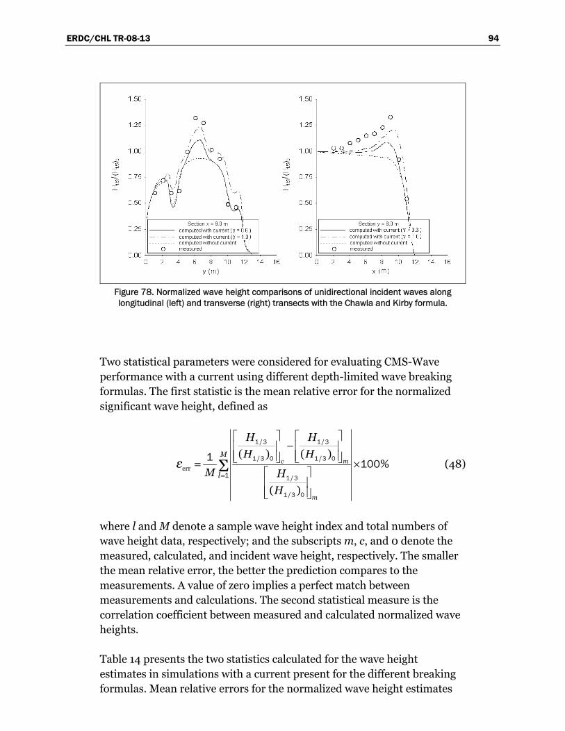
ERDC/CHL TR-08-13 94
Figure 78. Normalized wave height comparisons of unidirectional incident waves along longitudinal (left) and transverse (right) transects with the Chawla and Kirby formula.
Two statistical parameters were considered for evaluating CMS-Wave performance with a current using different depth-limited wave breaking formulas. The first statistic is the mean relative error for the normalized significant wave height, defined as
/ /
/ /
err
/
/
( ) ( )%
( )
Σ c m
m
M
l
H H
H H
M H
H
ε
1 3 1 3
1 3 0 1 3 0
1 3
1 3 0
1
1 100=
⎡ ⎤ ⎡ ⎤−⎢ ⎥ ⎢ ⎥
⎢ ⎥ ⎢ ⎥⎣ ⎦ ⎣ ⎦= ×⎡ ⎤⎢ ⎥⎢ ⎥⎣ ⎦
(48)
where l and M denote a sample wave height index and total numbers of wave height data, respectively; and the subscripts m, c, and 0 denote the measured, calculated, and incident wave height, respectively. The smaller the mean relative error, the better the prediction compares to the measurements. A value of zero implies a perfect match between measurements and calculations. The second statistical measure is the correlation coefficient between measured and calculated normalized wave heights.
Table 14 presents the two statistics calculated for the wave height estimates in simulations with a current present for the different breaking formulas. Mean relative errors for the normalized wave height estimates
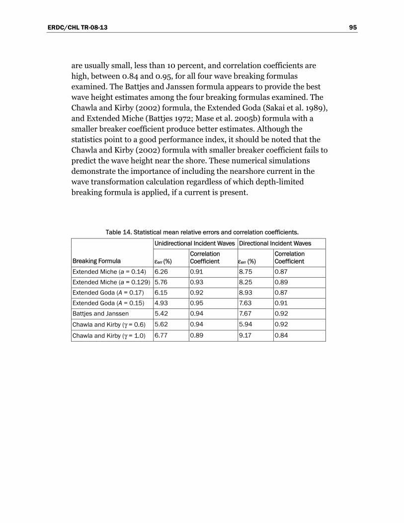
ERDC/CHL TR-08-13 95
are usually small, less than 10 percent, and correlation coefficients are high, between 0.84 and 0.95, for all four wave breaking formulas examined. The Battjes and Janssen formula appears to provide the best wave height estimates among the four breaking formulas examined. The Chawla and Kirby (2002) formula, the Extended Goda (Sakai et al. 1989), and Extended Miche (Battjes 1972; Mase et al. 2005b) formula with a smaller breaker coefficient produce better estimates. Although the statistics point to a good performance index, it should be noted that the Chawla and Kirby (2002) formula with smaller breaker coefficient fails to predict the wave height near the shore. These numerical simulations demonstrate the importance of including the nearshore current in the wave transformation calculation regardless of which depth-limited breaking formula is applied, if a current is present.
Table 14. Statistical mean relative errors and correlation coefficients.
Unidirectional Incident Waves Directional Incident Waves
Breaking Formula εerr (%) Correlation Coefficient εerr (%)
Correlation Coefficient
Extended Miche (a = 0.14) 6.26 0.91 8.75 0.87 Extended Miche (a = 0.129) 5.76 0.93 8.25 0.89 Extended Goda (A = 0.17) 6.15 0.92 8.93 0.87 Extended Goda (A = 0.15) 4.93 0.95 7.63 0.91 Battjes and Janssen 5.42 0.94 7.67 0.92
Chawla and Kirby (γ = 0.6) 5.62 0.94 5.94 0.92
Chawla and Kirby (γ = 1.0) 6.77 0.89 9.17 0.84
ERDC/CHL TR-08-13 96
5 Field Applications Field applications are presented for three locations: (1) Matagorda Bay,
TX; (2) Grays Harbor Entrance, WA; and (3) Southeast Oahu Coast, HI.
CMS-Wave calculations are compared to measurements to examine model
performance.
Matagorda Bay
Matagorda Bay is located on the north-central coast of Texas. The surface area of the bay is approximately 930 km2 with the depth between 2 to 4 m. The tidal prism of the bay is large because of the large bay surface area, despite having a modest tidal range of about 0.33 m in the bay. The bay is separated from the Gulf of Mexico by Matagorda Island and Matagorda Peninsula. Freshwater discharge, which originates mainly from the Colorado River and the Lavaca River, is less than 10 percent of the daily tidal exchange through the two inlets with Gulf of Mexico. Local wind is the dominant forcing for wave generation in the bay (Kraus et al. 2006).
Directional wave and water level data were collected by a bottom-mounted Acoustic Doppler Profiler (ADP) in 3.8 m of water for September to December 2005, at a middle bay location. The coordinates of this wave measurement station, MBWAV, are 28°31.285’N, 96°24.423’W. Local wind and tide data are available from NOAA sta 87737011 at Port O’Connor (28°26.8’N, 96°23.8’W) in the southwest corner of the bay. Figure 79 shows the wind, tide, and wave data-collection locations. Figures 80 and 81 show the hourly wind, tide, and wave data collected in September-December 2005. Water level data collected from MBWAV and Port O’Connor show that the spatial variation of water level in the bay can be significant under the passage of a front system and strong wind.
Waves generated by the wind are overall small to moderate in the middle of the bay during the data-collection period. Four large-wave events of interest observed in the data were produced by relatively strong wind, greater than 10 m/sec. Large waves were generated on 24 September 2005 under the strong wind of Hurricane Rita. The other three large wave events that occurred on 24 October, 1 November, and 15 November 2005, were produced by cold fronts. These large waves were generated by a wind directed between north and north-northeast. CMS-Wave simulations were
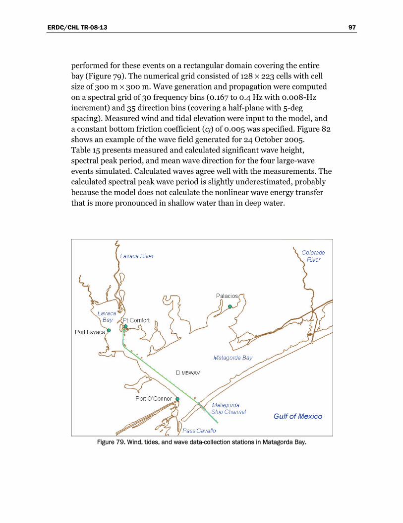
ERDC/CHL TR-08-13 97
performed for these events on a rectangular domain covering the entire bay (Figure 79). The numerical grid consisted of 128 × 223 cells with cell size of 300 m × 300 m. Wave generation and propagation were computed on a spectral grid of 30 frequency bins (0.167 to 0.4 Hz with 0.008-Hz increment) and 35 direction bins (covering a half-plane with 5-deg spacing). Measured wind and tidal elevation were input to the model, and a constant bottom friction coefficient (cf) of 0.005 was specified. Figure 82 shows an example of the wave field generated for 24 October 2005. Table 15 presents measured and calculated significant wave height, spectral peak period, and mean wave direction for the four large-wave events simulated. Calculated waves agree well with the measurements. The calculated spectral peak wave period is slightly underestimated, probably because the model does not calculate the nonlinear wave energy transfer that is more pronounced in shallow water than in deep water.
Figure 79. Wind, tides, and wave data-collection stations in Matagorda Bay.
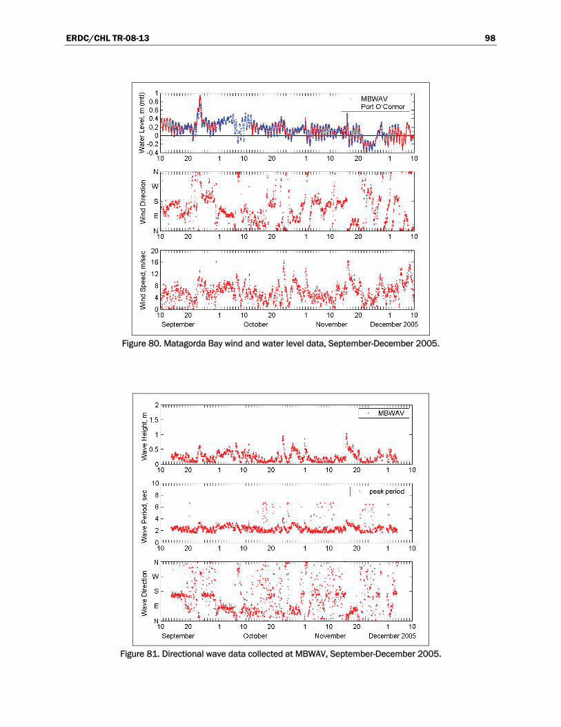
ERDC/CHL TR-08-13 98
Figure 80. Matagorda Bay wind and water level data, September-December 2005.
Figure 81. Directional wave data collected at MBWAV, September-December 2005.
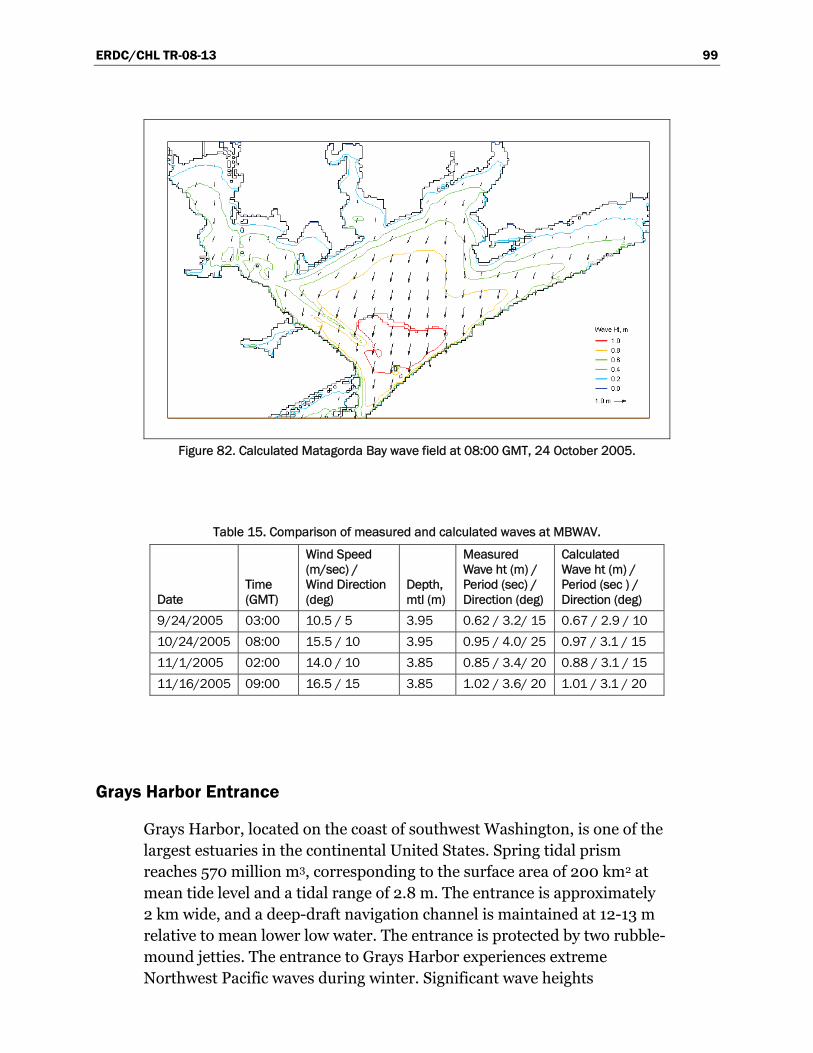
ERDC/CHL TR-08-13 99
Figure 82. Calculated Matagorda Bay wave field at 08:00 GMT, 24 October 2005.
Table 15. Comparison of measured and calculated waves at MBWAV.
Date Time (GMT)
Wind Speed (m/sec) / Wind Direction (deg)
Depth, mtl (m)
Measured Wave ht (m) / Period (sec) / Direction (deg)
Calculated Wave ht (m) / Period (sec ) / Direction (deg)
9/24/2005 03:00 10.5 / 5 3.95 0.62 / 3.2/ 15 0.67 / 2.9 / 10 10/24/2005 08:00 15.5 / 10 3.95 0.95 / 4.0/ 25 0.97 / 3.1 / 15 11/1/2005 02:00 14.0 / 10 3.85 0.85 / 3.4/ 20 0.88 / 3.1 / 15 11/16/2005 09:00 16.5 / 15 3.85 1.02 / 3.6/ 20 1.01 / 3.1 / 20
Grays Harbor Entrance
Grays Harbor, located on the coast of southwest Washington, is one of the largest estuaries in the continental United States. Spring tidal prism reaches 570 million m3, corresponding to the surface area of 200 km2 at mean tide level and a tidal range of 2.8 m. The entrance is approximately 2 km wide, and a deep-draft navigation channel is maintained at 12-13 m relative to mean lower low water. The entrance is protected by two rubble-mound jetties. The entrance to Grays Harbor experiences extreme Northwest Pacific waves during winter. Significant wave heights
ERDC/CHL TR-08-13 100
commonly exceed 6 m in winter storms. Strong ebb currents that exist between the jetties can increase wave height by as much as 0.5 to 1.5 m as observed in the inlet entrance.
Strong wave refraction and diffraction at the eastern end of the south jetty contribute to increased beach erosion in Half Moon Bay. To examine the influence of waves and currents in Half Moon Bay, wave and current data were collected at four stations between December 2003 and February 2004. Table 16 presents the location of four measurement stations (Osborne and Davies 2004). During the same time intervals, offshore wave information is available from a Coastal Data Information Program (CDIP) Buoy 036 (46°51.39’N, 124°14.67’W) in water of 40 m (mtl) and from National Data Buoy Center (NDBC) Buoy 46029 (46°8.63’N, 124°30.7’W), located approximately 100 km south-southeast of Grays Harbor. Ocean surface wind measurements are also available from Buoy 46029. Figure 83 shows the location map and local data-collection stations (Buoy 46029 and Half Moon Bay stations HMB1 to HMB4).
CMS-Wave simulations were conducted on a model grid of 440 × 600 cells, with cell size of 30 m × 30 m (Figure 83). Directional wave spectra from CDIP 036 served as the input, discretized in 30 frequency bins (0.04 to 0.33 Hz with 0.01-Hz increment) and 35 direction bins (5-deg spacing of a half-plane), at the seaward boundary. Five days of wave data over 24-28 December 2003 were analyzed for comparison to the calculation (Osborne and Davies 2004). A winter storm occurred during this 5-day interval with the largest offshore measured wave height exceeding 6 m. CMS-Wave was run in steering at 3-hr interval with the CMS-Flow to account for the influence of waves with current and tides. A diffraction intensity value of 2 and a forward reflection coefficient of 0.3 were specified. A constant bottom friction coefficient (cf) of 0.005 was specified in the model. Figure 84 shows the wave measurements at NDBC 46029 and CDIP 036 for 24-29 December 2003.
CMS-Wave was run to examine three different conditions: (1) wave transformation only, (2) wave transformation including local wind input, and (3) coupling with CMS-Flow (with wind, tide, and wave-current interaction). Figures 85 and 86 show calculated maximum current fields during the peak flood and ebb cycles, respectively, in the 5-day wave simulation coupled with the CMS-Flow. Figures 87 to 90 compare calculated results to the measurements. Because the offshore wave likely has reached the fully developed sea under the mild wind condition in the
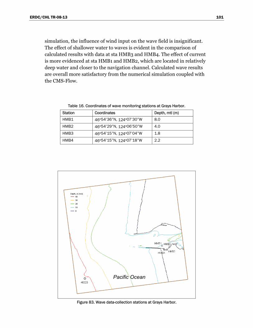
ERDC/CHL TR-08-13 101
simulation, the influence of wind input on the wave field is insignificant. The effect of shallower water to waves is evident in the comparison of calculated results with data at sta HMB3 and HMB4. The effect of current is more evidenced at sta HMB1 and HMB2, which are located in relatively deep water and closer to the navigation channel. Calculated wave results are overall more satisfactory from the numerical simulation coupled with the CMS-Flow.
Table 16. Coordinates of wave monitoring stations at Grays Harbor.
Station Coordinates Depth, mtl (m) HMB1 46o54’36”N, 124o07’30”W 8.0
HMB2 46o54’29”N, 124o06’50”W 4.0
HMB3 46o54’15”N, 124o07’04”W 1.8
HMB4 46o54’15”N, 124o07’18”W 2.2
Pacific OceanPacific Ocean
Figure 83. Wave data-collection stations at Grays Harbor.
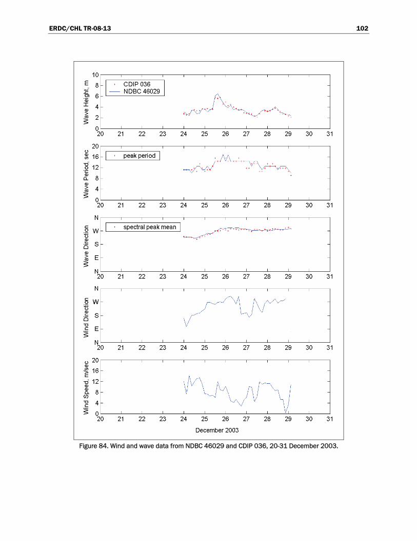
ERDC/CHL TR-08-13 102
Figure 84. Wind and wave data from NDBC 46029 and CDIP 036, 20-31 December 2003.
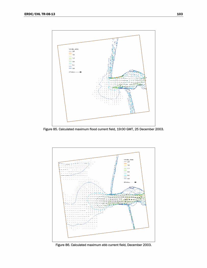
ERDC/CHL TR-08-13 103
Figure 85. Calculated maximum flood current field, 19:00 GMT, 25 December 2003.
Figure 86. Calculated maximum ebb current field, December 2003.
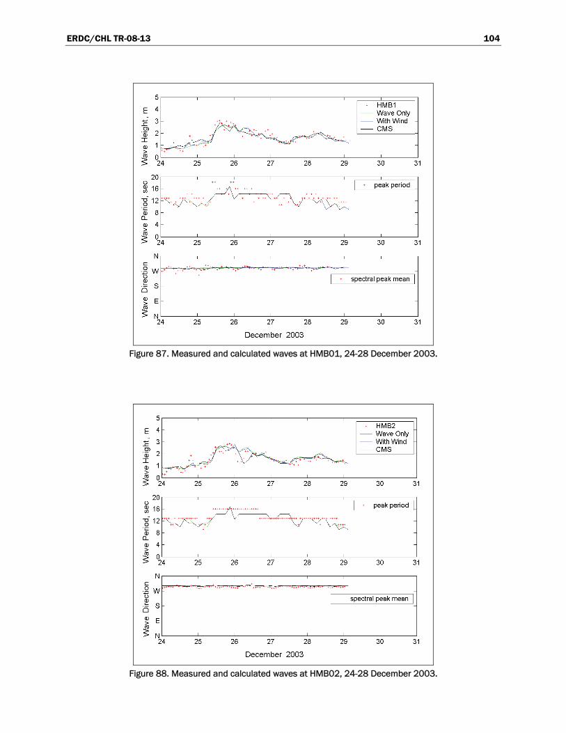
ERDC/CHL TR-08-13 104
Figure 87. Measured and calculated waves at HMB01, 24-28 December 2003.
Figure 88. Measured and calculated waves at HMB02, 24-28 December 2003.
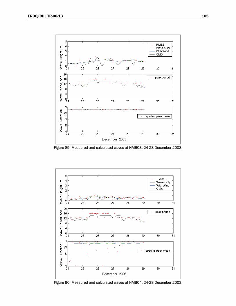
ERDC/CHL TR-08-13 105
Figure 89. Measured and calculated waves at HMB03, 24-28 December 2003.
Figure 90. Measured and calculated waves at HMB04, 24-28 December 2003.
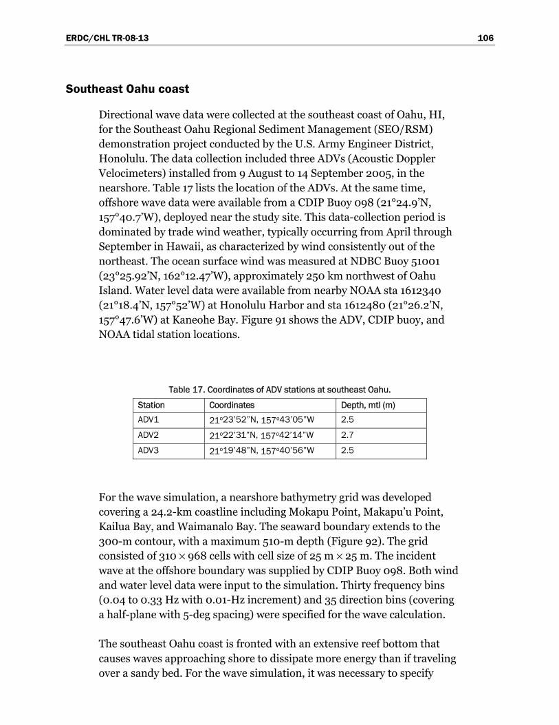
ERDC/CHL TR-08-13 106
Southeast Oahu coast
Directional wave data were collected at the southeast coast of Oahu, HI, for the Southeast Oahu Regional Sediment Management (SEO/RSM) demonstration project conducted by the U.S. Army Engineer District, Honolulu. The data collection included three ADVs (Acoustic Doppler Velocimeters) installed from 9 August to 14 September 2005, in the nearshore. Table 17 lists the location of the ADVs. At the same time, offshore wave data were available from a CDIP Buoy 098 (21°24.9’N, 157°40.7’W), deployed near the study site. This data-collection period is dominated by trade wind weather, typically occurring from April through September in Hawaii, as characterized by wind consistently out of the northeast. The ocean surface wind was measured at NDBC Buoy 51001 (23°25.92’N, 162°12.47’W), approximately 250 km northwest of Oahu Island. Water level data were available from nearby NOAA sta 1612340 (21°18.4’N, 157°52’W) at Honolulu Harbor and sta 1612480 (21°26.2’N, 157°47.6’W) at Kaneohe Bay. Figure 91 shows the ADV, CDIP buoy, and NOAA tidal station locations.
Table 17. Coordinates of ADV stations at southeast Oahu.
Station Coordinates Depth, mtl (m) ADV1 21o23’52”N, 157o43’05”W 2.5
ADV2 21o22’31”N, 157o42’14”W 2.7
ADV3 21o19’48”N, 157o40’56”W 2.5
For the wave simulation, a nearshore bathymetry grid was developed covering a 24.2-km coastline including Mokapu Point, Makapu’u Point, Kailua Bay, and Waimanalo Bay. The seaward boundary extends to the 300-m contour, with a maximum 510-m depth (Figure 92). The grid consisted of 310 × 968 cells with cell size of 25 m × 25 m. The incident wave at the offshore boundary was supplied by CDIP Buoy 098. Both wind and water level data were input to the simulation. Thirty frequency bins (0.04 to 0.33 Hz with 0.01-Hz increment) and 35 direction bins (covering a half-plane with 5-deg spacing) were specified for the wave calculation.
The southeast Oahu coast is fronted with an extensive reef bottom that causes waves approaching shore to dissipate more energy than if traveling over a sandy bed. For the wave simulation, it was necessary to specify
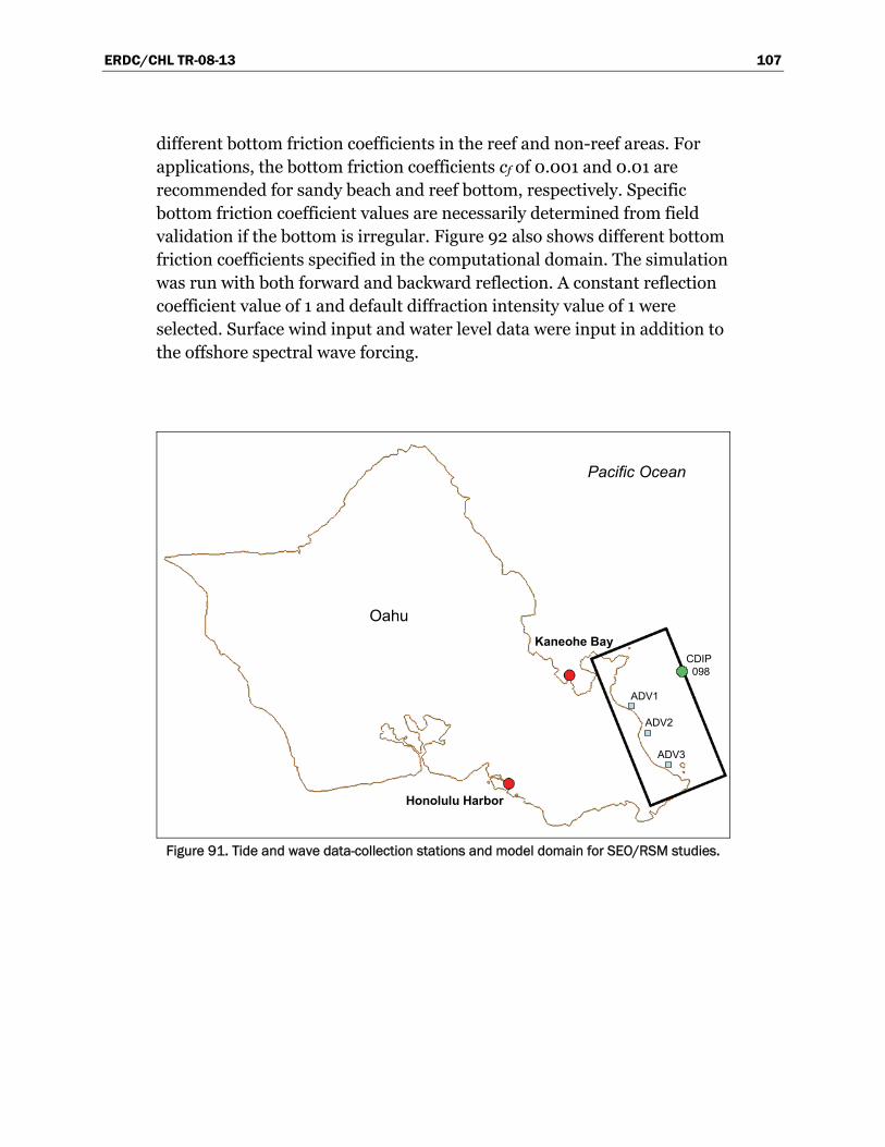
ERDC/CHL TR-08-13 107
different bottom friction coefficients in the reef and non-reef areas. For applications, the bottom friction coefficients cf of 0.001 and 0.01 are recommended for sandy beach and reef bottom, respectively. Specific bottom friction coefficient values are necessarily determined from field validation if the bottom is irregular. Figure 92 also shows different bottom friction coefficients specified in the computational domain. The simulation was run with both forward and backward reflection. A constant reflection coefficient value of 1 and default diffraction intensity value of 1 were selected. Surface wind input and water level data were input in addition to the offshore spectral wave forcing.
Honolulu Harbor
Kaneohe Bay
ADV1
ADV2
ADV3
CDIP098
Oahu
Pacific Ocean
Honolulu Harbor
Kaneohe Bay
ADV1
ADV2
ADV3
CDIP098
Oahu
Honolulu Harbor
Kaneohe Bay
ADV1
ADV2
ADV3
CDIP098
Oahu
Pacific Ocean
Figure 91. Tide and wave data-collection stations and model domain for SEO/RSM studies.
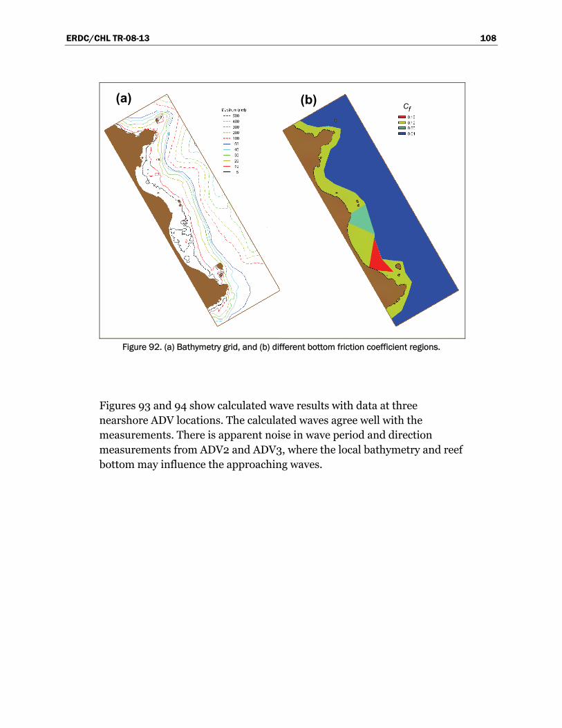
ERDC/CHL TR-08-13 108
(a)Cf
(b)(a)Cf
(b)
Figure 92. (a) Bathymetry grid, and (b) different bottom friction coefficient regions.
Figures 93 and 94 show calculated wave results with data at three nearshore ADV locations. The calculated waves agree well with the measurements. There is apparent noise in wave period and direction measurements from ADV2 and ADV3, where the local bathymetry and reef bottom may influence the approaching waves.
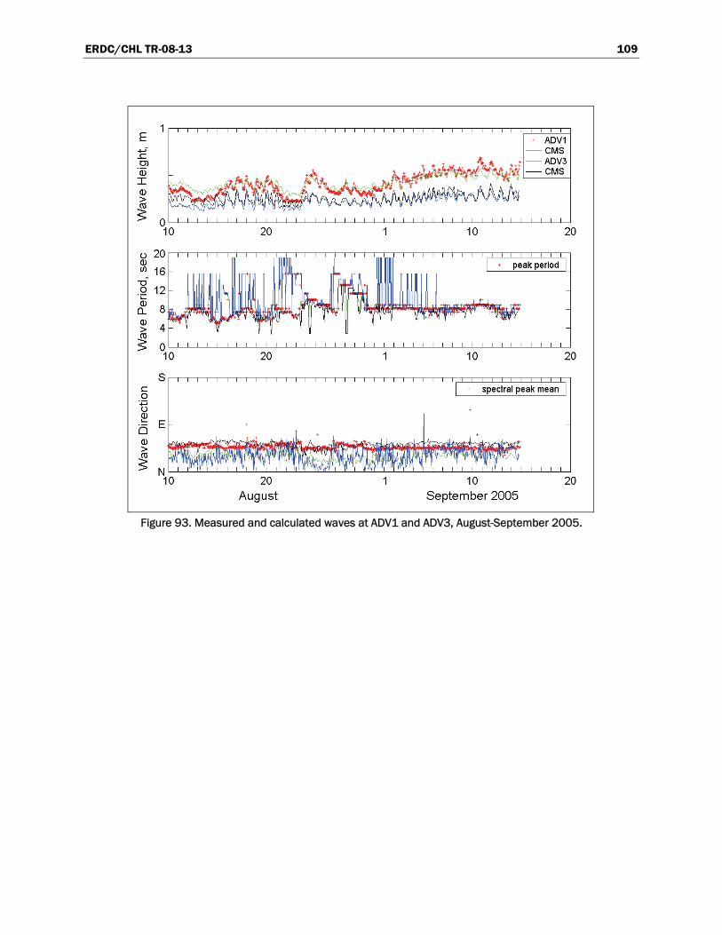
ERDC/CHL TR-08-13 109
Figure 93. Measured and calculated waves at ADV1 and ADV3, August-September 2005.
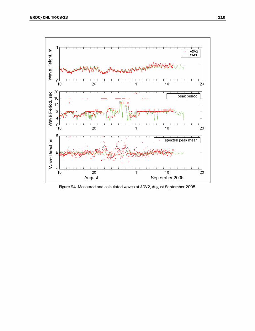
ERDC/CHL TR-08-13 110
Figure 94. Measured and calculated waves at ADV2, August-September 2005.
ERDC/CHL TR-08-13 111
References Ahrens, J. P., and M. S. Heimbaugh. 1988. Approximate upper limit of irregular wave
runup on riprap. Coastal Engineering Research Center Technical Report CERC-88-5. Vicksburg, MS: U.S. Army Engineer Waterways Experiment Station.
Ahrens, J. P., and M. F. Titus. 1981. Laboratory data report: irregular wave runup on plane smooth slopes. Coastal Engineering Research Center unpublished Laboratory Report. Vicksburg, MS: U.S. Army Engineer Waterways Experiment Station.
Battjes, J. A. 1972. Set-up due to irregular waves. Proceedings 13th International Conference on Coastal Engineering, ASCE, 1993-2004.
Battjes, J. A., and J. Janssen. 1978. Energy loss and set-up due to breaking of random waves. Proceedings 16th International Conference Coastal Engineering, ASCE, 569-587.
Booij, N., R. C. Ris, and L. H. Holthuijsen. 1999. A third-generation wave model for coastal regions: 1. Model description and validation. Journal of Geophysical Research 104(C4):7,649-7,666.
Bouws, E., and G. J. Komen. 1983. On the balance between growth and dissipation in extreme, depth limited wind-sea in the southern North Sea. Journal of Physical Oceanography 13:1,653-1,658.
Bretherton, F. P., and C. J. R. Garrett. 1968. Wave trains in inhomogeneous moving media. Proceedings Royal Society of London A(302):529-554.
Briggs, M. J., and P.L.-F. Liu. 1993. Experimental study on monochromatic wave-ebb current interaction. Proceedings 2nd International Symposium of Ocean Wave Measurement and Analysis, Waves 93, ASCE, 474-488.
Briggs, M. J., and Z. Demirbilek. 1996. Wave-current interaction in inlets. Proceedings 25th Coastal Engineering Conference, ASCE, 1,219-1,232.
Buttolph, A. M., C. W. Reed, N. C. Kraus, N. Ono, M. Larson, B. Camenen, H. Hanson, T. Wamsley, and A. Zundel. 2006. Two-dimensional depth-averaged circulation model CMS-M2D: Version 3.0: Report 2, sediment transport and morphology change. Coastal and Hydraulics Laboratory Technical Report ERDC/CHL TR-06-9. Vicksburg, MS: U.S. Army Engineer Research and Development Center.
Chawla A., and J. T. Kirby. 2002. Monochromatic and random wave breaking at blocking points. Journal of Geophysical Research 107(C7), 10.1029/2001JC001042.
Chen, W., V. G. Panchang, and Z. Demirbilek. 2005. On the modeling of wave-current interaction using the elliptic mild-slope wave equation. Ocean Engineering 32(17-18):2,135-2,164.
Collins, J. I. 1972. Prediction of shallow water spectra. Journal of Geophysical Research 77(15):2693-2707.
ERDC/CHL TR-08-13 112
Dally, W. R., R. G. Dean, and R. A. Dalrymple. 1985. Wave height variation across beaches of arbitrary profile. Journal of Geophysical Research 90(C6):11,917-11,927.
Dean, R. G. 1977. Equilibrium beach profiles: U.S. Atlantic and Gulf Coasts. Ocean Engineering Technical Report No. 12. Newark, DE: Department of Civil Engineering and College of Marine Studies, University of Delaware.
Dean, R. G., and R. A. Dalrymple. 1984. Water wave mechanics for engineers and scientitists. Englewood Cliffs, NJ: Prentice-Hall, Inc.
Demirbilek, Z., L. Lin, and O.G. Nwogu. 2008. Wave modeling for jetty rehabilitation at the Mouth of the Columbia River, Washington/Oregon, USA. Coastal and Hydraulics Laboratory Technical Report ERDC/CHL TR-08-3. Vicksburg, MS: U.S. Army Engineer Research and Development Center.
Demirbilek, Z., L. Lin, and A. Zundel. 2007. WABED model in the SMS: Part 2. Graphical interface. Coastal and Hydraulics Laboratory Engineering Technical Note ERDC/CHL CHETN-I-74. Vicksburg, MS: U.S. Army Engineer Research and Development Center.
Demirbilek, Z., and V. Panchang. 1998. CGWAVE: A coastal surface-water wave model of the mild-slope equation. Coastal and Hydraulics Laboratory Technical Report CHL-98-26. Vicksburg, MS: U.S. Army Engineer Waterways Experiment Station.
Goda, Y. 1970. A synthesis of breaker indices. Transactions of the Japan Society of Civil Engineers 13:227-230 (in Japanese).
Goda, Y. 1985. Random seas and design of maritime structures. Tokyo: University of Tokyo Press.
Goda, Y. 2006. Examination of the influence of several factors on longshore current computation with random waves. Coastal Engineering 53(2-3):157-170.
Guza, R. T., and E. B. Thornton. 1981. Wave set-up on a natural beach. Journal of Geophysical Research 86(C5):4,133-4,137.
Hardy, T. A. 1993. The attenuation of spectral transformation of wind waves on a coral reef. Queendsland, Australia: James Cook University of North Queensland, Townsville, 336 p.
Hasselmann, K., T. P. Barnett, E. Bouws, H. Carlson, D. E. Cartwright, K. Enke, J. A. Ewing, H. Gienapp, D. E. Hasselmann, P. Kruseman, A. Meerbrug, P. Muller, D. J. Olbers, K. Richter, W. Sell, and H. Walden. 1973. Measurements of wind-wave growth and swell decay during the Joint North Sea Wave Project (JONSWAP). Deutsche Hydrographische Zeitschrift A80(12), 95 p.
Headquarters, U.S. Army Corps of Engineers. 2002. Coastal Engineering Manual. EM 1110-2-1100. Washington, DC (in 6 volumes).
Hearn, C. J. 1999. Wave-breaking hydrodynamics within coral reef systems and the effect of changing relative sea level. Journal of Geophysical Research 104(C12):30,007-30,019.
ERDC/CHL TR-08-13 113
Hedges, T. S., K. Anastasiou, and D. Gabriel. 1985. Interaction of random waves and currents. Journal of Waterway, Port, Coastal, and Ocean Engineering 111(2):275-288, ASCE.
Holthuijsen, L. H., A. Herman, and N. Booij. 2004. Phase-decoupled refraction-diffraction for spectral wave models. Journal of Coastal Engineering 49:291-305.
Huang, N. E., D. T. Chen, C. C. Tung and J. R. Smith. 1972. Interactions between steady non-uniform currents and gravity waves with application for current instruments. Journal of Physical Oceanography 2:420-431.
Iwagaki, Y., T. Asano, Y. Yamanaka, and F. Nagai. 1980. Wave breaking due to currents. Annual Journal of Coastal Engineering 27:30-34, JSCE (in Japanese).
Jenkins, A. D., and O. M. Phillips. 2001. A simple formula for nonlinear wave-wave interaction. Journal of Offshore and Polar Engineering 11(2):81-86.
Johnson, J. W. 1952. Generalized wave diffraction diagrams. Proceedings 2nd Conference on Coastal Engineering, ASCE.
Jonsson, I. G. 1990. Wave-current interactions. Chapter 7, The Sea. B. Le Mehaute and D. Hanes (ed.). New York, NY: John Wiley and Sons, 65-120.
Komar, P. D. 1998. Beach processes and sedimentation. 2nd ed. Upper Saddle River, NJ: Prentice-Hall, Inc.
Komen, G. J., S. Hasselrnann, and K. Hasselmam. 1984. On the existence of a fully developed wind-sea spectrum. Journal of Physical Oceanography 14:1,271-1,285.
Kraus, N. C., L. Lin, B. K. Batten, and G. L. Brown. 2006. Matagorda Ship Channel, Texas: jetty stability study. Coastal and Hydraulics Laboratory Technical Report ERDC/CHL TR-06-7. Vicksburg, MS: U.S. Army Engineer Research and Development Center.
Lai, R. J., S. R. Long, and N. E. Huang. 1989. Laboratory studies of wave-current interaction: Kinematics of the strong interaction. Journal of Geophysical Research 97(C11):16,201-16,214.
Larson, M., and N. C. Kraus. 2002. NMLONG: Numerical model for simulating longshore current. Coastal and Hydraulics Laboratory Technical Report ERDC/CHL TR-02-22. Vicksburg, MS: U.S. Army Engineer Research and Development Center.
Li, Y., and G. Dong. 1993. Breaking of irregular waves with opposing current. Marine Science Bulletin 12(5):1-8 (in Chinese).
Lin, L., and Z. Demirbilek. 2005. Evaluation of two numerical wave models with inlet physical model. Journal of Waterway, Port, Coastal, and Ocean Engineering 131(4):149-161, ASCE.
Lin, L., and R.-Q. Lin. 2004a. Wave Breaking Function. Proceedings 8th International Workshop on Wave Hindcasting and Prediction. Oahu, Hawaii: North Shore. November 14-19.
ERDC/CHL TR-08-13 114
Lin, R.-Q., and L. Lin. 2004b. Wind Input Function. Proceedings 8th International Workshop on Wave Hindcasting and Prediction. North Shore, Oahu, Hawaii. November 14-19.
Lin, L., R.-Q. Lin, and J. P.-Y. Maa. 2006a. Numerical simulation of wind wave field. 9th International Workshop on Wave Hindcasting and Prediction. Victoria, British Columbia, Canada, 24-29 September.
Lin, L., H. Mase, F. Yamada, and Z. Demirbilek. 2006b. Wave-action balance equation diffraction (WABED) model: Tests of wave diffraction and reflection at inlets. Coastal and Hydraulics Engineering Technical Note ERDC/CHL CHETN-III-73. Vicksburg, MS: U.S. Army Engineer Research and Development Center.
Longuet-Higgins, M. S., and R. W. Stewart. 1961. The changes in amplitude of short gravity waves on steady non-uniform currents. Journal of Fluid Mechanics 10(4):529-549.
Lowe, R. J., J. L. Falter, M. D. Bandet, G. Pawlak, M. J. Atkinson, S. G. Monismith, J. R. Koseff. 2005. Spectal wave dissipation over a barrier reef. Journal of Geophysical Research 110(C04001), doi:10.1029/2004JC002711, 16 p.
Macagno, E. O. 1953. Houle dans un can presentent un passage en charge. La Houille Blanche 9(1):10–37.
Mase, H. 2001. Multidirectional random wave transformation model based on energy balance equation. Coastal Engineering Journal 43(4):317-337 JSCE.
Mase, H. 1989. Random wave runup height on gentle slope. Journal of Waterway, Port, Coastal, and Ocean Engineering 85(3):123-152, ASCE.
Mase, H., H. Amamori, and T. Takayama. 2005a. Wave prediction model in wave-current coexisting field. Proceedings 12th Canadian Coastal Conference (CD-ROM).
Mase, H., and Y. Iwagaki. 1984. Runup of random waves on gentle slopes. Proceedings 19th International Conference on Coastal Engineering, ASCE, 593-609.
Mase, H., and T. Kitano. 2000. Spectrum-based prediction model for random wave transformation over arbitrary bottom topography. Coastal Engineering Journal 42(1):111-151, JSCE.
Mase, H., K. Oki, T. S. Hedges, and H. J. Li. 2005b. Extended energy-balance-equation wave model for multidirectional random wave transformation. Ocean Engineering 32(8-9):961-985.
Miche, M. 1951. Le pouvoir reflechissant des ouvrages maritimes exposes a 1’action de la houle. Annals des Ponts et Chau.ssess. 121e Annee: 285-319 (translated by Lincoln and Chevron, University of California, Berkeley, Wave Research Laboratory, Series 3, Issue 363, June 1954).
Mitsuyasu, H., and T. Honda. 1982. Wind-induced growth of water waves. Journal of Fluid Mechanics 123:425-442.
ERDC/CHL TR-08-13 115
Nwogu, O., and Z. Demirbilek. 2001. BOUSS-2D: A Boussinesq wave model for coastal regions and harbors. Coastal and Hydraulics Laboratory Technical Report ERDC/CHL TR-01-25. Vicksburg, MS: U.S. Army Engineer Research and Development Center.
Osborne P. D., and M. H. Davies. 2004. South jetty sediment processes study, Grays Harbor, Washington: Processes along Half Moon Bay. PIE Technical Report. Edmonds, WA: Pacific International Engineering.
Osborne, P. D., and N. J. MacDonald. 2005. Wave energy evaluation of passenger only ferries in Rich Passage. FTA Report FTA-WA-26-7007-2005. Washington, DC: Federal Transit Administration, U.S. Department of Transportation.
Ostendorf, D. W., and O. S. Madsen. 1979. An analysis of longshore currents and associated sediment transport in the surf zone. Report No. MITSG 79-13. Cambridge, MA: Massachusetts Institute of Technology, 169 p.
Phillips, O. M. 1957. On the generation of waves by turbulent wind. Journal of Fluid Mechanics 2:417-445.
Raichlen, F. 1993. Wave propagating on an adverse jet. Proceedings 2nd International Symposium of Ocean Wave Measurement and Analysis, Waves 93, ASCE, 657-670.
Ris, R. C., and L. H. Holthuijsen. 1996. Spectral modeling of current induced wave-blocking. Proceedings 25th Coastal Engineering Conference, ASCE, 1,247-1,254.
Rivero, F. J., A. S. Arcilla, and E. Carci. 1997. An analysis of diffraction in spectral wave models. Proceedings 3rd International Symposium of Ocean Wave Measurement and Analysis, Waves 97, ASCE, 431–445.
Sakai, S., N. Kobayashi, and K. Koike. 1989. Wave breaking criterion with opposing current on sloping bottom: an extension of Goda’s breaker index. Annual Journal of Coastal Engineering 36:56-59, JSCE (in Japanese).
Seabergh, W. C., W. R. Curtis, L. J. Thomas, and K. K. Hathaway. 2002. Physical model study of wave diffraction-refraction at an idealized inlet. Coastal Inlet Research Program Technical Report ERDC/CHL-TR-02-27. Vicksburg, MS: U.S. Army Engineer Research and Development Center.
Seabergh, W. C., L. Lin, and Z. Demirbilek. 2005. Laboratory study of hydrodynamics near absorbing and fully reflecting jetties. Coastal and Hydraulics Laboratory Technical Report ERDC/CHL TR-05-8. Vicksburg, MS: U.S. Army Engineer Research and Development Center.
Shore protection manual. 1984. 4th ed., 2 Vol, U.S. Army Engineer Waterways Experiment Station, U.S. Government Printing Office, Washington, DC.
Smith, J. M. 2001a. Breaking in a spectral wave model. Proceedings 4th International Symposium of Ocean Wave Measurement and Analysis, Waves 01, ASCE, 1,022-1,031.
Smith, J. M. 2001b. Modeling nearshore transformation with STWAVE. Coastal and Hydraulics Laboratory Special Report ERDC/CHL SR-01-01. Vicksburg, MS: U.S. Army Engineer Research and Development Center.
ERDC/CHL TR-08-13 116
Smith, J. M., D. T. Resio, and A. Zundel. 1999. STWAVE: Steady-state spectral wave model, Report 1: User’s manual for STWAVE Version 2.0. Coastal and Hydraulics Laboratory Instruction Report CHL-99-1. Vicksburg, MS: U.S. Army Engineer Waterways Experiment Station.
Smith, J. M., W. C. Seabergh, G. S. Harkins, and M. J. Briggs. 1998. Wave breaking on a current at an idealized inlet. Coastal and Hydraulics Laboratory Technical Report CHL-98-31. Vicksburg, MS: U.S. Army Engineer Waterways Experiment Station.
Suh, K. D., Y. Y. Kim, and D. Y. Lee. 1994. Equilibrium-range spectrum of waves propagating on currents. Journal of Waterway, Port, Coastal, and Ocean Engineering 120(5):434-450, ASCE.
Takayama, T., Ikeda, N., Hiraishi, T. 1991. Wave transformation calculation considering wave breaking and reflection. Technical Report, Port Harbor Research Institute, Japan 30 (1): 21-67.
Tayfun, M. A., R. A. Dalrymple, and C. Y. Yang. 1976. Random wave-current interaction in water of varying depth. Ocean Engineering, Vol.3:403-420.
Thornton, E. B., and R. T. Guza. 1983. Transformation of wave height distribution. Journal of Geophysical Research 88(C10):5,925-5,938.
Visser, P. J. 1991. Laboratory measurements of uniform longshore currents. Coastal Engineering 15:563-593.
Whitham, G. B. 1974. Linear and nonlinear waves. New York, NY: John Wiley.
Wiegel, R. L. 1962. Diffraction of waves by a semi-infinite breakwater. Journal of the Hydraulics Division 88(HY1):27-44.
Yu, Y. Y. 1950. Breaking of waves by opposing current. Transaction of American Geophysical Union 33(1):39-41.
Zhao, L., V. G. Panchang, W. Chen, Z. Demirbilek, and N. Chhabbra. 2001. Simulation of breaking effects in a two dimensional harbor wave prediction model. Coastal Engineering 42:359-373.
Zheng, J., H. Mase, Z. Demirbilek, and L. Lin. 2008. Implementation and evaluation of alternative wave breaking formulas in a coastal spectral wave model. Ocean Engineering (in press).
Zubier, K., V. G. Panchang, and Z. Demirbilek. 2003. Simulation of waves at Duck (North Carolina) using two numerical models. Coastal Engineering Journal 45(3):439-469.
Zundel, A. 2006. Surface-water modeling system reference manual – Version 9.2. Provo, UT: Brigham Young University Environmental Modeling Research Laboratory.
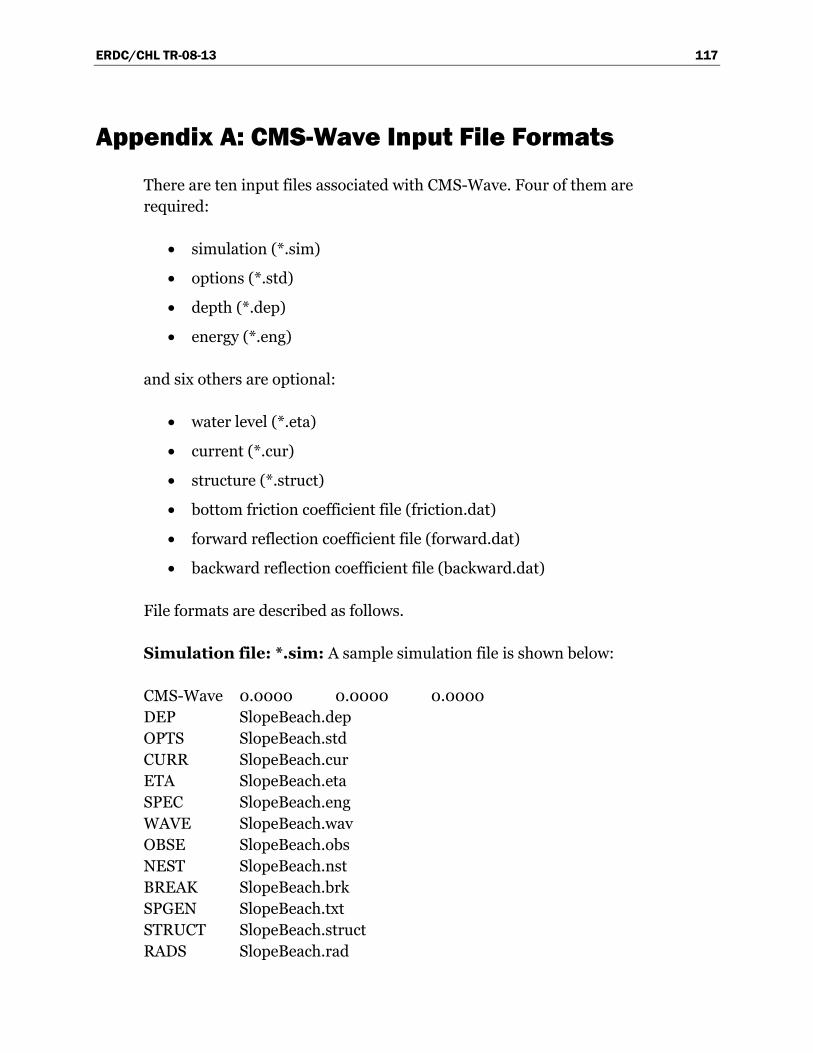
ERDC/CHL TR-08-13 117
Appendix A: CMS-Wave Input File Formats
There are ten input files associated with CMS-Wave. Four of them are required:
• simulation (*.sim)
• options (*.std)
• depth (*.dep)
• energy (*.eng)
and six others are optional:
• water level (*.eta)
• current (*.cur)
• structure (*.struct)
• bottom friction coefficient file (friction.dat)
• forward reflection coefficient file (forward.dat)
• backward reflection coefficient file (backward.dat)
File formats are described as follows.
Simulation file: *.sim: A sample simulation file is shown below:
CMS-Wave 0.0000 0.0000 0.0000 DEP SlopeBeach.dep OPTS SlopeBeach.std CURR SlopeBeach.cur ETA SlopeBeach.eta SPEC SlopeBeach.eng WAVE SlopeBeach.wav OBSE SlopeBeach.obs NEST SlopeBeach.nst BREAK SlopeBeach.brk SPGEN SlopeBeach.txt STRUCT SlopeBeach.struct RADS SlopeBeach.rad
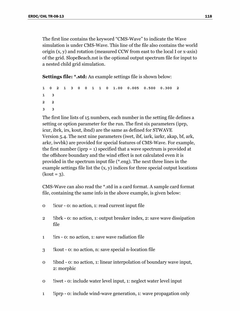
ERDC/CHL TR-08-13 118
The first line contains the keyword “CMS-Wave” to indicate the Wave simulation is under CMS-Wave. This line of the file also contains the world origin (x, y) and rotation (measured CCW from east to the local I or x-axis) of the grid. SlopeBeach.nst is the optional output spectrum file for input to a nested child grid simulation.
Settings file: *.std: An example settings file is shown below:
1 0 2 1 3 0 0 1 1 0 1.00 0.005 0.500 0.300 2
1 3
2 2
3 3
The first line lists of 15 numbers, each number in the setting file defines a setting or option parameter for the run. The first six parameters (iprp, icur, ibrk, irs, kout, ibnd) are the same as defined for STWAVE Version 5.4. The next nine parameters (iwet, ibf, iark, iarkr, akap, bf, ark, arkr, iwvbk) are provided for special features of CMS-Wave. For example, the first number (iprp = 1) specified that a wave spectrum is provided at the offshore boundary and the wind effect is not calculated even it is provided in the spectrum input file (*.eng). The next three lines in the example settings file list the (x, y) indices for three special output locations (kout = 3).
CMS-Wave can also read the *.std in a card format. A sample card format file, containing the same info in the above example, is given below:
0 !icur - 0: no action, 1: read current input file
2 !ibrk - 0: no action, 1: output breaker index, 2: save wave dissipation file
1 !irs - 0: no action, 1: save wave radiation file
3 !kout - 0: no action, n: save special n-location file
0 !ibnd - 0: no action, 1: linear interpolation of boundary wave input, 2: morphic
0 !iwet - 0: include water level input, 1: neglect water level input
1 !iprp - 0: include wind-wave generation, 1: wave propagation only
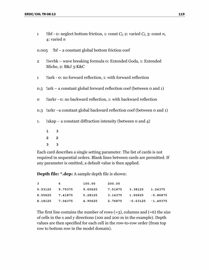
ERDC/CHL TR-08-13 119
1 !ibf - 0: neglect bottom friction, 1: const Cf, 2: varied Cf, 3: const n, 4: varied n
0.005 !bf – a constant global bottom friction coef
2 !iwvbk – wave breaking formula 0: Extended Goda, 1: Extended Miche, 2: B&J 3:K&C
1 !iark - 0: no forward reflection, 1: with forward reflection
0.5 !ark – a constant global forward reflection coef (between 0 and 1)
0 !iarkr - 0: no backward reflection, 1: with backward reflection
0.3 !arkr –a constant global backward reflection coef (between 0 and 1)
1. !akap – a constant diffraction intensity (between 0 and 4)
1 3
2 2
3 3
Each card describes a single setting parameter. The list of cards is not required in sequential orders. Blank lines between cards are permitted. If any parameter is omitted, a default value is then applied.
Depth file: *.dep: A sample depth file is shown:
3 6 100.00 200.00
9.93125 9.79375 9.65625 7.51875 3.38125 1.24375
8.55625 7.41875 5.28125 3.14375 1.00625 -0.86875
8.18125 7.04375 4.90625 2.76875 -0.63125 -1.49375
The first line contains the number of rows (=3), columns and (=6) the size of cells in the x and y directions (100 and 200 m in the example). Depth values are then specified for each cell in the row-to-row order (from top row to bottom row in the model domain).
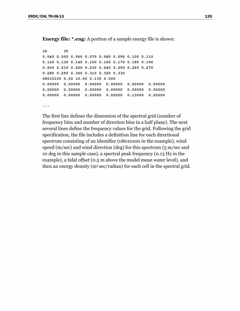
ERDC/CHL TR-08-13 120
Energy file: *.eng: A portion of a sample energy file is shown:
30 35
0.040 0.050 0.060 0.070 0.080 0.090 0.100 0.110
0.120 0.130 0.140 0.150 0.160 0.170 0.180 0.190
0.200 0.210 0.220 0.230 0.240 0.250 0.260 0.270
0.280 0.290 0.300 0.310 0.320 0.330
08010100 5.00 10.00 0.130 0.500
0.00000 0.00000 0.00000 0.00000 0.00000 0.00000
0.00000 0.00000 0.00000 0.00000 0.00000 0.00000
0.00000 0.00000 0.00000 0.02000 0.13000 0.25000
...
The first line defines the dimension of the spectral grid (number of frequency bins and number of direction bins in a half plane). The next several lines define the frequency values for the grid. Following the grid specification, the file includes a definition line for each directional spectrum consisting of an identifier (08010100 in the example), wind speed (m/sec) and wind direction (deg) for this spectrum (5 m/sec and 10 deg in this sample case), a spectral peak frequency (0.13 Hz in the example), a tidal offset (0.5 m above the model mean water level), and then an energy density (m2 sec/radian) for each cell in the spectral grid.
REPORT DOCUMENTATION PAGE Form Approved
OMB No. 0704-0188 Public reporting burden for this collection of information is estimated to average 1 hour per response, including the time for reviewing instructions, searching existing data sources, gathering and maintaining the data needed, and completing and reviewing this collection of information. Send comments regarding this burden estimate or any other aspect of this collection of information, including suggestions for reducing this burden to Department of Defense, Washington Headquarters Services, Directorate for Information Operations and Reports (0704-0188), 1215 Jefferson Davis Highway, Suite 1204, Arlington, VA 22202-4302. Respondents should be aware that notwithstanding any other provision of law, no person shall be subject to any penalty for failing to comply with a collection of information if it does not display a currently valid OMB control number. PLEASE DO NOT RETURN YOUR FORM TO THE ABOVE ADDRESS.
1. REPORT DATE (DD-MM-YYYY) August 2008
2. REPORT TYPE Final report
3. DATES COVERED (From - To)
5a. CONTRACT NUMBER
5b. GRANT NUMBER
4. TITLE AND SUBTITLE
CMS-Wave: A Nearshore Spectral Wave Processes Model for Coastal Inlets and Navigation Projects
5c. PROGRAM ELEMENT NUMBER
5d. PROJECT NUMBER
5e. TASK NUMBER
6. AUTHOR(S)
Lihwa Lin, Zeki Demirbilek, Hajime Mase, Jinhai Zheng, and Fumihiko Yamada
5f. WORK UNIT NUMBER
7. PERFORMING ORGANIZATION NAME(S) AND ADDRESS(ES) 8. PERFORMING ORGANIZATION REPORT NUMBER U.S. Army Engineer Research and Development Center, Coastal and Hydraulics Laboratory
3909 Halls Ferry Road, Vicksburg, MS 39180-6199; Disaster Prevention Research Institute, Kyoto University, Gokasho, Uji, Kyoto, 611-0011, JAPAN; Hohai University, Research Institute of Coastal and Ocean Engineering, 1 Xikang Road, Nanjing, 210098, China; Kumamato University, Graduate School of Science and Technology, 2-39-1, Kurokami, Kumamoto, 860-8555, JAPAN
ERDC/CHL TR-08-13
9. SPONSORING / MONITORING AGENCY NAME(S) AND ADDRESS(ES) 10. SPONSOR/MONITOR’S ACRONYM(S)
11. SPONSOR/MONITOR’S REPORT NUMBER(S)
Headquarters, U.S. Army Corps of Engineers, Washington, DC 20314-1000; U.S. Army Engineer Research and Development Center, Coastal and Hydraulics Laboratory 3909 Halls Ferry Road, Vicksburg, MS 39180-6199 12. DISTRIBUTION / AVAILABILITY STATEMENT Approved for public release; distribution is unlimited.
13. SUPPLEMENTARY NOTES
14. ABSTRACT The Coastal Inlets Research Program (CIRP) of the U.S. Army Engineer Research and Development Center, Coastal and Hydraulics Laboratory, in collaboration with two universities in Japan, has developed a spectral wave transformation numerical model to address needs of the U.S. Army Corps of Engineers navigation projects. The model is called CMS-Wave and is part of Coastal Modeling System (CMS) developed in the CIRP. The CMS is a suite of coupled models operated in the Surface-water Modeling System (SMS), which is an interactive and comprehensive graphical user interface environment for preparing model input, running models, and viewing and analyzing results. CMS-Wave is designed for accurate and reliable representation of wave processes affecting operation and maintenance of coastal inlet structures in navigation projects as well as in risk and reliability assessment of shipping in inlets and harbors. Important wave processes at coastal inlets are diffraction, refraction, reflection, wave breaking, and dissipation mechanisms, and the wave-current interaction. The effect of locally-generated wind can also be significant during wave propagation at inlets. This report provides information on CMS-Wave theory, numerical implementation, and SMS interface. A set of examples are given to demonstrate the model’s applicability for storm-damage assessment, modification to jetties including jetty extensions, jetty breaching, addition of spurs to inlet jetties, and planning and design of nearshore reefs and barrier islands to protect beaches and promote navigation reliability.
15. SUBJECT TERMS coastal inlet jetty
model nearshore simulation
Spectral wave
16. SECURITY CLASSIFICATION OF: 17. LIMITATION OF ABSTRACT
18. NUMBER OF PAGES
19a. NAME OF RESPONSIBLE PERSON
a. REPORT
UNCLASSIFIED
b. ABSTRACT
UNCLASSIFIED
c. THIS PAGE
UNCLASSIFIED 131 19b. TELEPHONE NUMBER (include area code)
Standard Form 298 (Rev. 8-98) Prescribed by ANSI Std. 239.18

![connell kraus.ppt [Read-Only] · Coastal and Hydraulics Laboratory Motivation • Need for predicting response of multiple-system, evolving coastal regions with interacting projects](https://static.fdocuments.net/doc/165x107/5e68d08c714c76622d25383d/connell-krausppt-read-only-coastal-and-hydraulics-laboratory-motivation-a-need.jpg)