April 2018

U.S. Energy Information Administration | Assumptions to the Annual Energy Outlook 2018: Coal Market Module 1

Coal Market Module The National Energy Modeling System (NEMS) Coal Market Module (CMM) provides projections of U.S. coal production, consumption, exports, imports, distribution, and prices. The CMM comprises three functional areas: coal production, coal distribution, and coal exports. A detailed description of the CMM is provided in the EIA publication, Coal Market Module of the National Energy Modeling System 2014, DOE/EIA-M060 (2014) (Washington, DC, 2014).

Key assumptions Coal production The CMM generates a different set of supply curves for each year of the projection. Combinations of 14 supply regions, 9 coal types (unique groupings of thermal grade and sulfur content), and 2 mine types (underground and surface) result in 41 separate supply curves. Supply curves are constructed using an econometric formulation that relates the mine mouth prices of coal for each supply curve to a set of independent variables. The independent variables include capacity utilization of mines, mining capacity, labor productivity, the user cost of capital of mining equipment, the cost of factor inputs (labor and fuel), and other mine supply costs.

The key assumptions underlying the coal production modeling are as follows:

• As capacity utilization increases, higher mine-mouth prices for a given supply curve are projected. The opportunity to add production capacity is allowed within the modeling framework if capacity utilization rises to a pre-determined level, typically in the 80% range. Likewise, if capacity utilization falls, mining capacity may be retired. The amount of capacity that can be added or retired in a given year depends on the supply region, the capacity utilization level, and the mining process (underground or surface). The volume of capacity expansion permitted in a projection year is based upon historical patterns of capacity additions.

• The wage rate for U.S. coal miners averaged $80,533 in 2015 [1]. For the Annual Energy Outlook 2018 (AEO2018), miner wages are assumed to remain flat in real terms (i.e., increase at the general rate of inflation) at the 2015 wage level. Mine equipment costs are also assumed to remain constant at the 2013 level over the projection period. The equipment index is built from the U.S. Bureau of Labor Statistics series for “Mining machinery and equipment” for underground mining and “Construction Machinery” for surface mining [2].

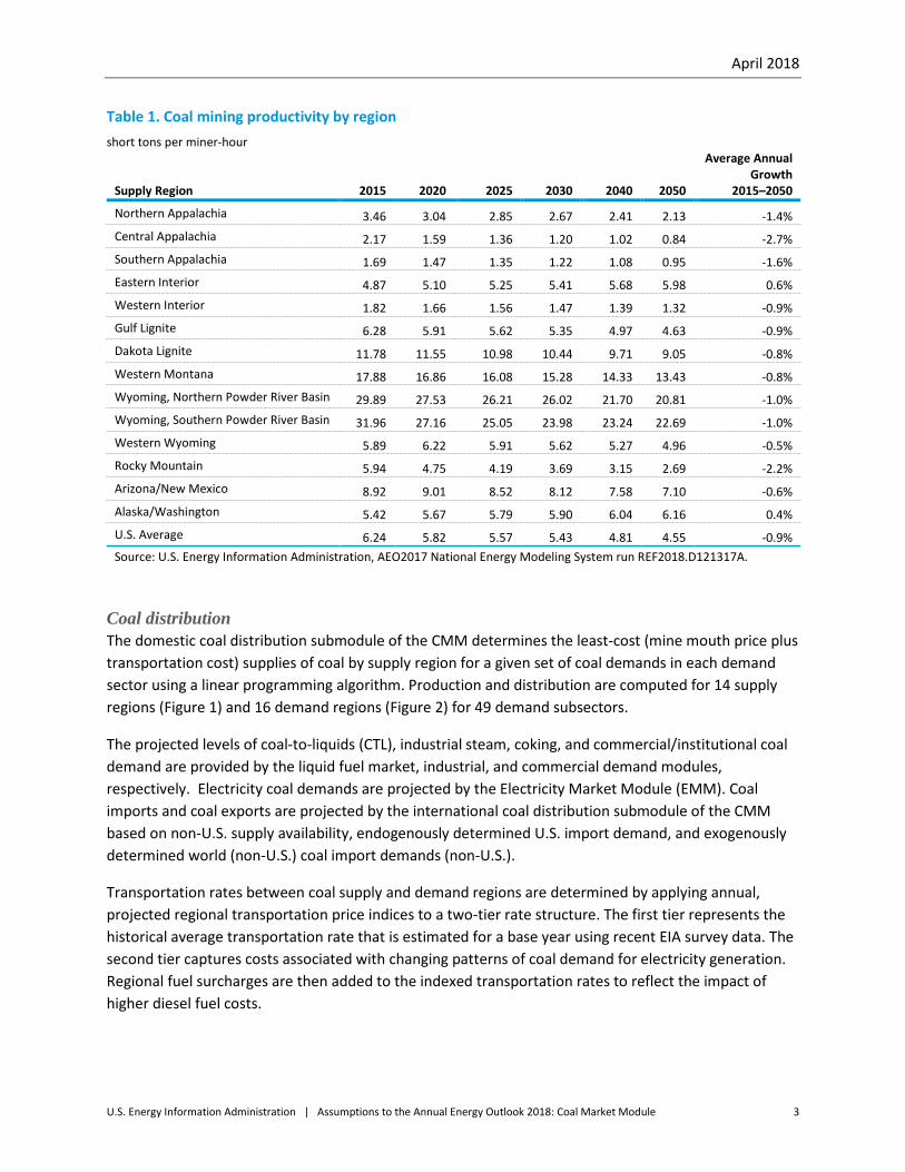
• In the CMM, different rates of labor productivity improvement or decline are assumed for each of the 41 coal supply curves used to represent U.S. coal supply. AEO2018 Reference case projections for regional coal mining productivity are provided in Table 1. Overall U.S. coal mining labor productivity declines at a rate of 0.9%/year between 2015 and 2050 in the Reference case. Higher stripping ratios at surface mines and the added labor needed to maintain more extensive underground mines offset productivity gains achieved from improved equipment, automation, and technology in most coal supply regions. Historical data on labor productivity are provided on a quarterly and annual basis by individual coal mines and preparation plants on the U.S. Department of Labor, Mine Safety and Health Administration’s Form 7000-2, “Quarterly Mine

April 2018

U.S. Energy Information Administration | Assumptions to the Annual Energy Outlook 2018: Coal Market Module 2

Employment and Coal Production Report,” and EIA’s Form EIA-7A, “Annual Survey of Coal Production and Preparation.”

• Between 1980 and 2000, U.S. coal mining labor productivity increased at an average rate of 6.6%/year, from 1.93 to 6.99 short tons per miner-hour. The major factors underlying these gains were inter-fuel price competition, structural change in the industry, and technological improvements in coal mining [3]. Between 2000 and 2015, growth in overall U.S. coal mining productivity has been negative in all CMM supply regions but three (Eastern Interior, Arizona/New Mexico, and Alaska/Washington), declining nationally at a rate of 0.8%/year to 6.24 short tons per miner-hour in 2015.

• Mine closures can sometimes result in small gains in regional productivity because the least productive mines are often those that suspend operation. On the other hand, highly productive mining operations can appear less productive when existing mine capacity is not fully utilized as has been the case in recent years. In 2015, 6 out of 14 coal supply regions showed productivity increases over 2014, while 1 remained flat and the rest showed productivity declines. However, the 2015 national average coal mining labor productivity rate of 6.24 short tons per miner-hour reflected a 12% increase over the 2014 productivity rate of 5.58 tons per miner-hour.

• Productivity in some areas of the coalfields in the eastern United States is projected to decline as operations move from mature coal fields to marginal reserve areas. In the Central Appalachian coal basin, which has been mined extensively, productivity declined by almost 50% between 2000 and 2015, corresponding to an average decline of 4.3%/year. Regulatory restrictions on surface mines and fragmentation of underground reserves limit the benefits that can be achieved by Appalachian producers from economies of scale. In 2015, Central Appalachia productivity fell to 2.17 short tons per miner-hour, only a 1.4% drop from 2014. However, the Central Appalachia region is projected to have the fastest regional decline in productivity at 2.7%/year from 2015 to 2050.

• Although declines have been more moderate at the highly-productive mines in Wyoming’s Powder River Basin (PRB), coal mining productivity in this region still fell by 31% between 2000 and 2015, corresponding to an average rate of decline of 2.4%/year. For AEO2017 onward, productivity figures for the PRB production areas were modified based on an assessment of recent private sector analyses [4]. In AEO2018 productivity in northern and southern PRB is projected to decline at an average rate of 1.0%/year from 2015 to 2050.

• The Eastern Interior has shown the best overall performance, with coal mining productivity growing by 3.2% between 2000 and 2015, or 0.2%/year. The Eastern Interior region, which has a substantial amount of thick, underground-minable coal reserves, is currently experiencing a resurgence in coal mining activity, with several coal companies operating highly productive longwall mines. Productivity is expected to increase modestly at a rate of 0.6%/year from 2015 to 2050.

April 2018

U.S. Energy Information Administration | Assumptions to the Annual Energy Outlook 2018: Coal Market Module 3

Table 1. Coal mining productivity by region short tons per miner-hour

Supply Region 2015 2020 2025 2030 2040 2050

Average Annual Growth

2015–2050

Northern Appalachia 3.46 3.04 2.85 2.67 2.41 2.13 -1.4% Central Appalachia 2.17 1.59 1.36 1.20 1.02 0.84 -2.7% Southern Appalachia 1.69 1.47 1.35 1.22 1.08 0.95 -1.6% Eastern Interior 4.87 5.10 5.25 5.41 5.68 5.98 0.6% Western Interior 1.82 1.66 1.56 1.47 1.39 1.32 -0.9% Gulf Lignite 6.28 5.91 5.62 5.35 4.97 4.63 -0.9% Dakota Lignite 11.78 11.55 10.98 10.44 9.71 9.05 -0.8% Western Montana 17.88 16.86 16.08 15.28 14.33 13.43 -0.8% Wyoming, Northern Powder River Basin 29.89 27.53 26.21 26.02 21.70 20.81 -1.0% Wyoming, Southern Powder River Basin 31.96 27.16 25.05 23.98 23.24 22.69 -1.0% Western Wyoming 5.89 6.22 5.91 5.62 5.27 4.96 -0.5% Rocky Mountain 5.94 4.75 4.19 3.69 3.15 2.69 -2.2% Arizona/New Mexico 8.92 9.01 8.52 8.12 7.58 7.10 -0.6% Alaska/Washington 5.42 5.67 5.79 5.90 6.04 6.16 0.4% U.S. Average 6.24 5.82 5.57 5.43 4.81 4.55 -0.9% Source: U.S. Energy Information Administration, AEO2017 National Energy Modeling System run REF2018.D121317A.

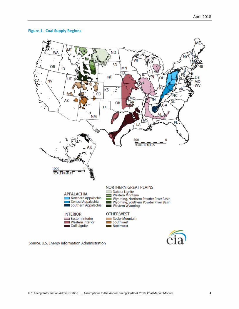
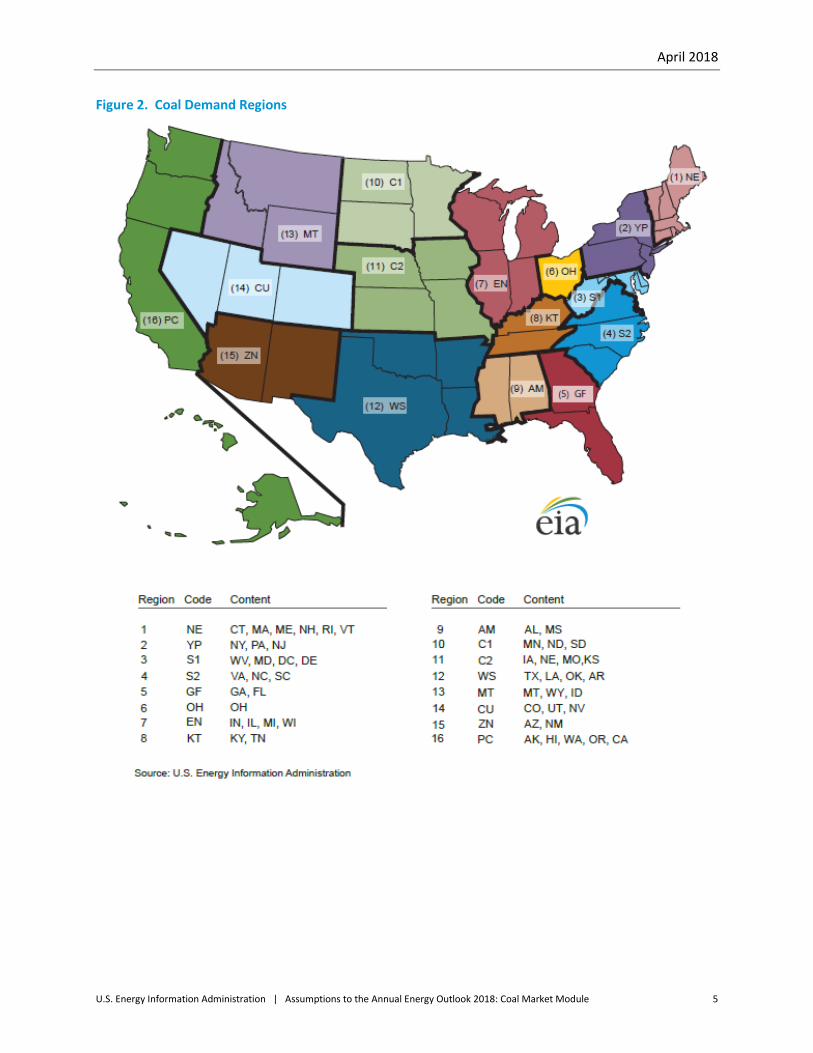
Coal distribution The domestic coal distribution submodule of the CMM determines the least-cost (mine mouth price plus transportation cost) supplies of coal by supply region for a given set of coal demands in each demand sector using a linear programming algorithm. Production and distribution are computed for 14 supply regions (Figure 1) and 16 demand regions (Figure 2) for 49 demand subsectors.

The projected levels of coal-to-liquids (CTL), industrial steam, coking, and commercial/institutional coal demand are provided by the liquid fuel market, industrial, and commercial demand modules, respectively. Electricity coal demands are projected by the Electricity Market Module (EMM). Coal imports and coal exports are projected by the international coal distribution submodule of the CMM based on non-U.S. supply availability, endogenously determined U.S. import demand, and exogenously determined world (non-U.S.) coal import demands (non-U.S.).

Transportation rates between coal supply and demand regions are determined by applying annual, projected regional transportation price indices to a two-tier rate structure. The first tier represents the historical average transportation rate that is estimated for a base year using recent EIA survey data. The second tier captures costs associated with changing patterns of coal demand for electricity generation. Regional fuel surcharges are then added to the indexed transportation rates to reflect the impact of higher diesel fuel costs.

April 2018

U.S. Energy Information Administration | Assumptions to the Annual Energy Outlook 2018: Coal Market Module 4

Figure 1. Coal Supply Regions

April 2018

U.S. Energy Information Administration | Assumptions to the Annual Energy Outlook 2018: Coal Market Module 5

Figure 2. Coal Demand Regions

April 2018

U.S. Energy Information Administration | Assumptions to the Annual Energy Outlook 2018: Coal Market Module 6

The key assumptions underlying the coal distribution modeling are as follows:

• Base-year (2015) transportation costs are estimates of average transportation costs for each origin-destination pair without differentiation by transportation mode (rail, truck, barge, and conveyor). These costs are computed as the difference between the average delivered price for a demand region (by sector and for export) and the average mine-mouth price for a supply curve. Delivered price data are from Form EIA-3, “Quarterly Coal Consumption and Quality Report, Manufacturing and Transformation/Processing Coal Plants and Commercial and Institutional Coal Users,” Form EIA-5, Quarterly Coal Consumption and Quality Report, Coke Plants,” Form EIA-923, “Power Plant Operations Report,” and the U.S. Bureau of the Census, “Monthly Report EM-545.” Mine mouth price data are from Form EIA-7A, “Coal Production and Preparation Report.”

• For the electricity sector only, a two-tier transportation rate structure is used for those regions which, in response to changing patterns of coal demand, may expand their market share beyond historical levels. The first-tier rate represents the historical average transportation rate. The second-tier transportation rate captures the higher cost of expanded shipping distances in large demand regions. The second tier is also captures costs associated with the use of subbituminous coal at units that were not originally designed for their use. This cost is estimated at $0.10/ million British thermal units (Btu) (2000 dollars) [5].

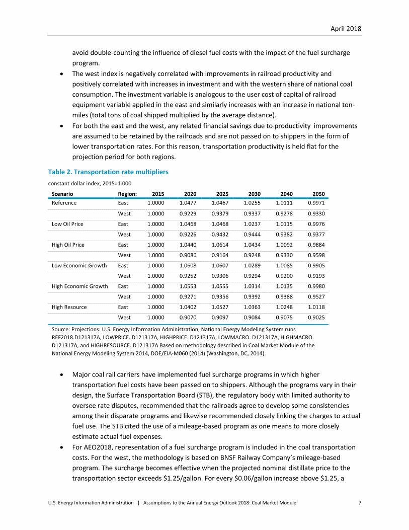
• Coal transportation costs, both first- and second-tier rates, are modified over time by two regional (east and west) transportation indices. The indices, calculated econometrically, measure of the change in average transportation rates for coal shipments on a tonnage basis, which occurs between successive years for coal shipments. An east index is used for coal originating from coal supply regions located east of the Mississippi River, while a west index is used for coal originating from coal supply regions located west of the Mississippi River. The indices are universally applied to all domestic coal transportation movements within the CMM. In the AEO2018 Reference case, both eastern and western coal transportation rates are projected to remain near their 2015 levels. The transportation rate indices for six AEO2018 cases are shown in Table 2, where the index value equals 1.00 for 2015.

• The east index is negatively correlated with improvements in railroad productivity, and it is positively correlated with the user cost of capital for railroad equipment and the national average diesel fuel price. The user cost of capital for railroad equipment is calculated from the producer price index (PPI) for railroad equipment and accounts for the opportunity cost of money used to purchase equipment and depreciation occurring as a result of use of the equipment (assumed at 10%), less any capital gain associated with the worth of the equipment. In calculating the user cost of capital, three percentage points are added to the cost of borrowing to account for the possibility that a national-level program to regulate greenhouse gas emissions may be implemented in the future. An increase in national ton-miles (total tons of coal shipped multiplied by the average distance) increases PPI and, consequently, the user cost of capital. Diesel fuel is removed from the equation for the east in the projection period to

April 2018

U.S. Energy Information Administration | Assumptions to the Annual Energy Outlook 2018: Coal Market Module 7

avoid double-counting the influence of diesel fuel costs with the impact of the fuel surcharge program.

• The west index is negatively correlated with improvements in railroad productivity and positively correlated with increases in investment and with the western share of national coal consumption. The investment variable is analogous to the user cost of capital of railroad equipment variable applied in the east and similarly increases with an increase in national ton-miles (total tons of coal shipped multiplied by the average distance).

• For both the east and the west, any related financial savings due to productivity improvements are assumed to be retained by the railroads and are not passed on to shippers in the form of lower transportation rates. For this reason, transportation productivity is held flat for the projection period for both regions.

Table 2. Transportation rate multipliers constant dollar index, 2015=1.000

Scenario Region: 2015 2020 2025 2030 2040 2050 Reference East 1.0000 1.0477 1.0467 1.0255 1.0111 0.9971

West 1.0000 0.9229 0.9379 0.9337 0.9278 0.9330

Low Oil Price East 1.0000 1.0468 1.0468 1.0237 1.0115 0.9976

West 1.0000 0.9226 0.9432 0.9444 0.9382 0.9377

High Oil Price East 1.0000 1.0440 1.0614 1.0434 1.0092 0.9884

West 1.0000 0.9086 0.9164 0.9248 0.9330 0.9598

Low Economic Growth East 1.0000 1.0608 1.0607 1.0289 1.0085 0.9905

West 1.0000 0.9252 0.9306 0.9294 0.9200 0.9193

High Economic Growth East 1.0000 1.0553 1.0555 1.0314 1.0135 0.9980

West 1.0000 0.9271 0.9356 0.9392 0.9388 0.9527

High Resource East 1.0000 1.0402 1.0527 1.0363 1.0248 1.0118

West 1.0000 0.9070 0.9097 0.9084 0.9075 0.9025

Source: Projections: U.S. Energy Information Administration, National Energy Modeling System runs REF2018.D121317A, LOWPRICE. D121317A, HIGHPRICE. D121317A, LOWMACRO. D121317A, HIGHMACRO. D121317A, and HIGHRESOURCE. D121317A Based on methodology described in Coal Market Module of the National Energy Modeling System 2014, DOE/EIA-M060 (2014) (Washington, DC, 2014).

• Major coal rail carriers have implemented fuel surcharge programs in which higher transportation fuel costs have been passed on to shippers. Although the programs vary in their design, the Surface Transportation Board (STB), the regulatory body with limited authority to oversee rate disputes, recommended that the railroads agree to develop some consistencies among their disparate programs and likewise recommended closely linking the charges to actual fuel use. The STB cited the use of a mileage-based program as one means to more closely estimate actual fuel expenses.

• For AEO2018, representation of a fuel surcharge program is included in the coal transportation costs. For the west, the methodology is based on BNSF Railway Company’s mileage-based program. The surcharge becomes effective when the projected nominal distillate price to the transportation sector exceeds $1.25/gallon. For every $0.06/gallon increase above $1.25, a

April 2018

U.S. Energy Information Administration | Assumptions to the Annual Energy Outlook 2018: Coal Market Module 8

$0.01/carload mile is charged. For the east, the methodology is based on CSX Transportation’s mileage-based program. The surcharge becomes effective when the projected nominal distillate price to the transportation sector exceeds $2.00/gallon. For every $0.04/gallon increase above $2.00, a $0.01/carload mile is charged. The number of tons per carload and the number of miles vary with each supply and demand region combination and are a pre-determined model input. The final calculated surcharge (in constant dollars per ton) is added to the escalator-adjusted transportation rate. For every projection year, 100% of all coal shipments are assumed to be subject to the surcharge program.

• Coal contracts in the CMM represent a minimum quantity of a specific electricity coal demand that must be met by a unique coal supply source prior to consideration of any alternative sources of supply. Base-year (2015) coal contracts between coal producers and electricity generators are estimated on the basis of receipts data reported by generators on the Form EIA-923, “Power Plant Operations Report.” Coal contracts are specified by CMM supply region, coal type, demand region, and whether or not a unit has flue gas desulfurization equipment. Coal contract quantities are reduced over time on the basis of contract duration data from information reported on the Form EIA-923, “Power Plant Operations Report,” historical patterns of coal use, and information obtained from various coal and electric power industry publications and reports.

• CTL facilities are assumed to be economic when low-sulfur distillate prices reach high enough levels. These plants are assumed to be co-production facilities with generation capacity of 832 megawatts (MW) (295 MW for the grid and 537 MW to support the conversion process) and the capability of producing 48,000 barrels/day of liquid fuels. The technology assumed is similar to an integrated gasification combined cycle, first converting the coal feedstock to gas and then subsequently converting the syngas to liquid hydrocarbons using the Fischer-Tropsch process. Of the total amount of coal consumed at each plant, 40% of the energy input is retained in the product with the remaining energy used for conversion and for the production of power sold to the grid. For AEO2018, coal-biomass-to-liquids (CBTL) are not modeled. CTL facilities produce distillate fuel oil (about 72%) and paraffinic naphtha used in plastics production and blend-able naphtha used in motor gasoline (together about 28% of the total by volume).

Coal imports and exports Coal imports and exports are modeled as part of the CMM’s linear program that provides an annual projection of U.S. steam and metallurgical coal exports in the context of world coal trade. The CMM projects steam and metallurgical coal trade flows from 17 coal-exporting regions of the world to 20 import regions for 2 coal types (steam and metallurgical), including 5 U.S. export regions and 4 U.S. import regions. The linear program determines the pattern of world coal trade flows that minimizes the production and transportation costs of meeting U.S. import demand and a pre-specified set of regional coal import demands, subject to constraints on export capacity and trade flows.

The key assumptions underlying coal export modeling are as follows:

• Coal buyers (importing regions) tend to spread their purchases among several suppliers to reduce the impact of potential supply disruptions, even though this may add to their purchase

April 2018

U.S. Energy Information Administration | Assumptions to the Annual Energy Outlook 2018: Coal Market Module 9

costs. Similarly, producers choose not to rely on any one buyer and instead endeavor to diversify their sales.

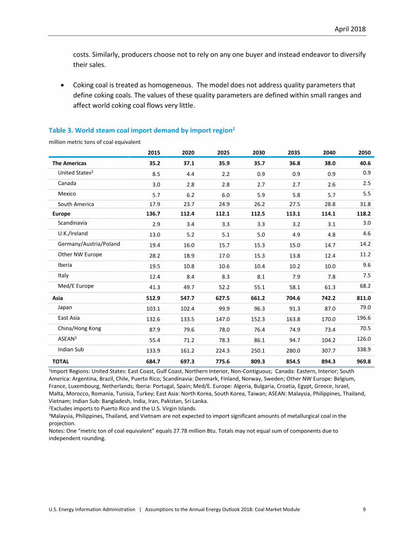
• Coking coal is treated as homogeneous. The model does not address quality parameters that define coking coals. The values of these quality parameters are defined within small ranges and affect world coking coal flows very little.

Table 3. World steam coal import demand by import region1 million metric tons of coal equivalent

2015 2020 2025 2030 2035 2040 2050

The Americas 35.2 37.1 35.9 35.7 36.8 38.0 40.6 United States2 8.5 4.4 2.2 0.9 0.9 0.9 0.9

Canada 3.0 2.8 2.8 2.7 2.7 2.6 2.5

Mexico 5.7 6.2 6.0 5.9 5.8 5.7 5.5

South America 17.9 23.7 24.9 26.2 27.5 28.8 31.8 Europe 136.7 112.4 112.1 112.5 113.1 114.1 118.2 Scandinavia 2.9 3.4 3.3 3.3 3.2 3.1 3.0

U.K./Ireland 13.0 5.2 5.1 5.0 4.9 4.8 4.6

Germany/Austria/Poland 19.4 16.0 15.7 15.3 15.0 14.7 14.2

Other NW Europe 28.2 18.9 17.0 15.3 13.8 12.4 11.2

Iberia 19.5 10.8 10.6 10.4 10.2 10.0 9.6

Italy 12.4 8.4 8.3 8.1 7.9 7.8 7.5

Med/E Europe 41.3 49.7 52.2 55.1 58.1 61.3 68.2

Asia 512.9 547.7 627.5 661.2 704.6 742.2 811.0 Japan 103.1 102.4 99.9 96.3 91.3 87.0 79.0

East Asia 132.6 133.5 147.0 152.3 163.8 170.0 196.6

China/Hong Kong 87.9 79.6 78.0 76.4 74.9 73.4 70.5

ASEAN3 55.4 71.2 78.3 86.1 94.7 104.2 126.0

Indian Sub 133.9 161.2 224.3 250.1 280.0 307.7 338.9

TOTAL 684.7 697.3 775.6 809.3 854.5 894.3 969.8 1Import Regions: United States: East Coast, Gulf Coast, Northern Interior, Non-Contiguous; Canada: Eastern, Interior; South America: Argentina, Brazil, Chile, Puerto Rico; Scandinavia: Denmark, Finland, Norway, Sweden; Other NW Europe: Belgium, France, Luxembourg, Netherlands; Iberia: Portugal, Spain; Med/E. Europe: Algeria, Bulgaria, Croatia, Egypt, Greece, Israel, Malta, Morocco, Romania, Tunisia, Turkey; East Asia: North Korea, South Korea, Taiwan; ASEAN: Malaysia, Philippines, Thailand, Vietnam; Indian Sub: Bangladesh, India, Iran, Pakistan, Sri Lanka. 2Excludes imports to Puerto Rico and the U.S. Virgin Islands. 3Malaysia, Philippines, Thailand, and Vietnam are not expected to import significant amounts of metallurgical coal in the projection. Notes: One “metric ton of coal equivalent” equals 27.78 million Btu. Totals may not equal sum of components due to independent rounding.

April 2018

U.S. Energy Information Administration | Assumptions to the Annual Energy Outlook 2018: Coal Market Module 10

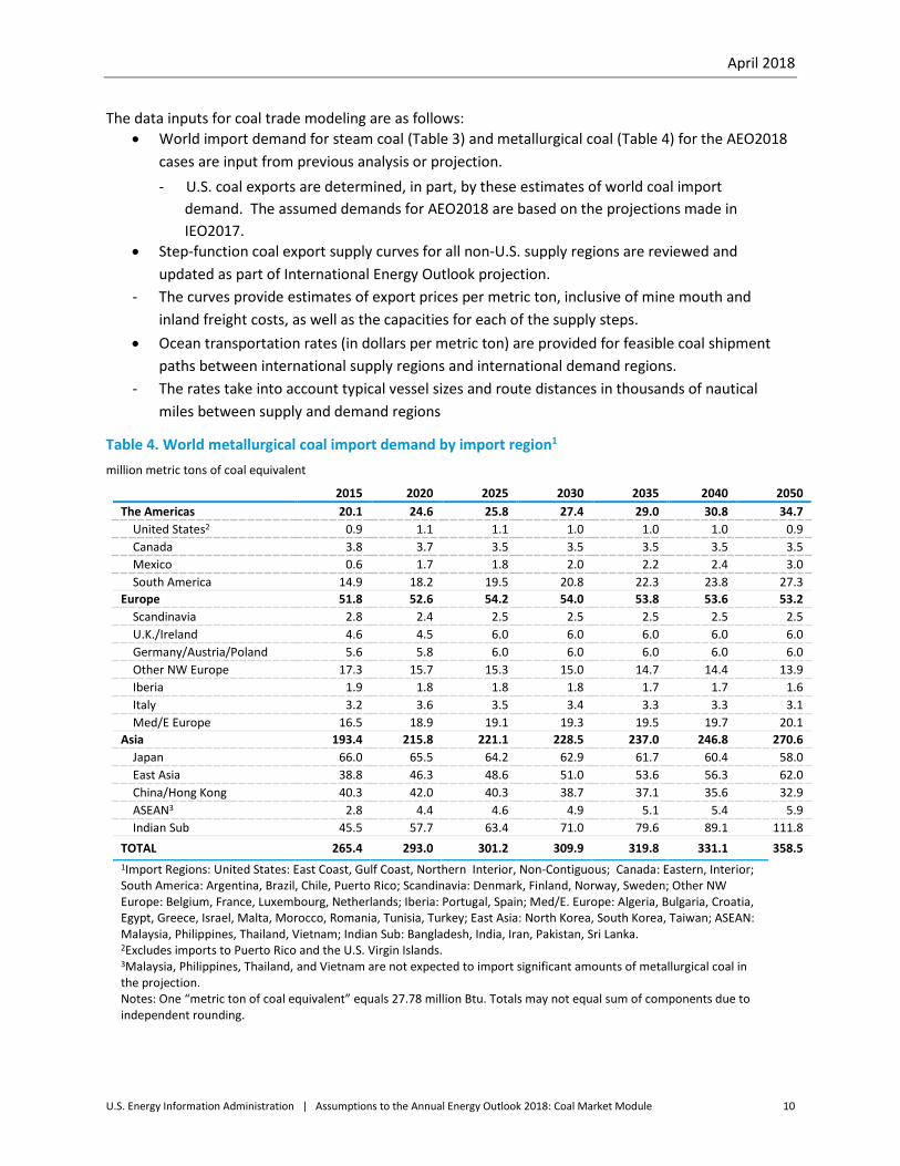
The data inputs for coal trade modeling are as follows: • World import demand for steam coal (Table 3) and metallurgical coal (Table 4) for the AEO2018

cases are input from previous analysis or projection. - U.S. coal exports are determined, in part, by these estimates of world coal import demand. The assumed demands for AEO2018 are based on the projections made in IEO2017.

• Step-function coal export supply curves for all non-U.S. supply regions are reviewed and updated as part of International Energy Outlook projection.

- The curves provide estimates of export prices per metric ton, inclusive of mine mouth and inland freight costs, as well as the capacities for each of the supply steps.

• Ocean transportation rates (in dollars per metric ton) are provided for feasible coal shipment paths between international supply regions and international demand regions.

- The rates take into account typical vessel sizes and route distances in thousands of nautical miles between supply and demand regions

Table 4. World metallurgical coal import demand by import region1

million metric tons of coal equivalent

2015 2020 2025 2030 2035 2040 2050 The Americas 20.1 24.6 25.8 27.4 29.0 30.8 34.7 United States2 0.9 1.1 1.1 1.0 1.0 1.0 0.9 Canada 3.8 3.7 3.5 3.5 3.5 3.5 3.5 Mexico 0.6 1.7 1.8 2.0 2.2 2.4 3.0 South America 14.9 18.2 19.5 20.8 22.3 23.8 27.3 Europe 51.8 52.6 54.2 54.0 53.8 53.6 53.2 Scandinavia 2.8 2.4 2.5 2.5 2.5 2.5 2.5 U.K./Ireland 4.6 4.5 6.0 6.0 6.0 6.0 6.0 Germany/Austria/Poland 5.6 5.8 6.0 6.0 6.0 6.0 6.0 Other NW Europe 17.3 15.7 15.3 15.0 14.7 14.4 13.9 Iberia 1.9 1.8 1.8 1.8 1.7 1.7 1.6 Italy 3.2 3.6 3.5 3.4 3.3 3.3 3.1 Med/E Europe 16.5 18.9 19.1 19.3 19.5 19.7 20.1 Asia 193.4 215.8 221.1 228.5 237.0 246.8 270.6 Japan 66.0 65.5 64.2 62.9 61.7 60.4 58.0 East Asia 38.8 46.3 48.6 51.0 53.6 56.3 62.0 China/Hong Kong 40.3 42.0 40.3 38.7 37.1 35.6 32.9 ASEAN3 2.8 4.4 4.6 4.9 5.1 5.4 5.9 Indian Sub 45.5 57.7 63.4 71.0 79.6 89.1 111.8 TOTAL 265.4 293.0 301.2 309.9 319.8 331.1 358.5 1Import Regions: United States: East Coast, Gulf Coast, Northern Interior, Non-Contiguous; Canada: Eastern, Interior; South America: Argentina, Brazil, Chile, Puerto Rico; Scandinavia: Denmark, Finland, Norway, Sweden; Other NW Europe: Belgium, France, Luxembourg, Netherlands; Iberia: Portugal, Spain; Med/E. Europe: Algeria, Bulgaria, Croatia, Egypt, Greece, Israel, Malta, Morocco, Romania, Tunisia, Turkey; East Asia: North Korea, South Korea, Taiwan; ASEAN: Malaysia, Philippines, Thailand, Vietnam; Indian Sub: Bangladesh, India, Iran, Pakistan, Sri Lanka. 2Excludes imports to Puerto Rico and the U.S. Virgin Islands. 3Malaysia, Philippines, Thailand, and Vietnam are not expected to import significant amounts of metallurgical coal in the projection. Notes: One “metric ton of coal equivalent” equals 27.78 million Btu. Totals may not equal sum of components due to independent rounding.

April 2018

U.S. Energy Information Administration | Assumptions to the Annual Energy Outlook 2018: Coal Market Module 11

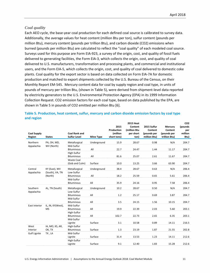
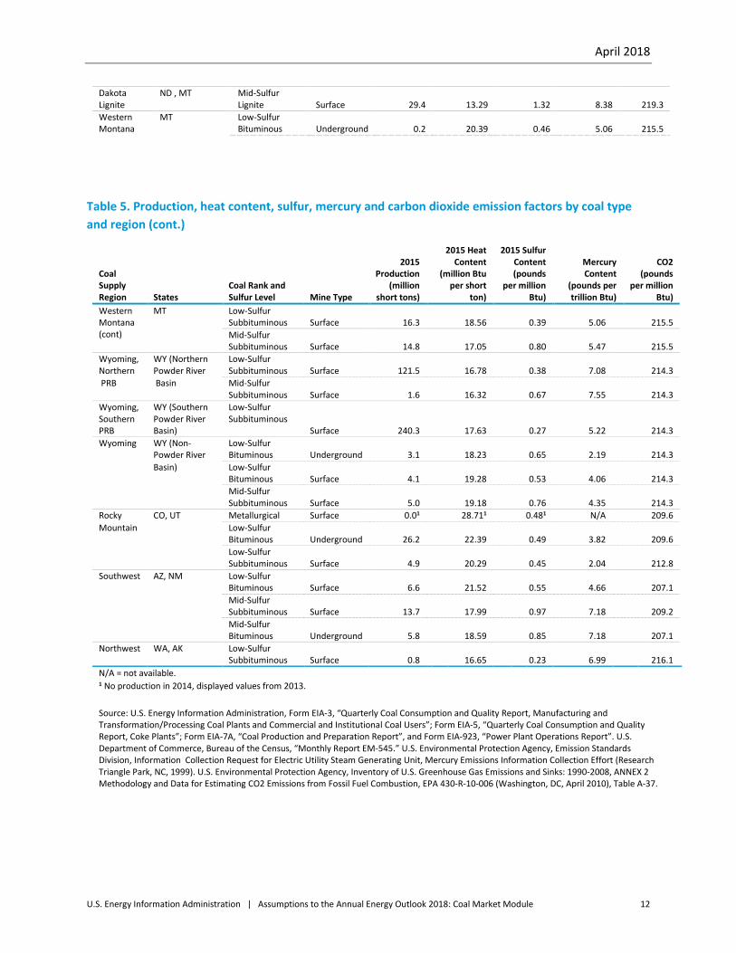
Coal quality Each AEO cycle, the base-year coal production for each defined coal source is calibrated to survey data. Additionally, the average values for heat content (million Btu per ton), sulfur content (pounds per million Btu), mercury content (pounds per trillion Btu), and carbon dioxide (CO2) emissions when burned (pounds per million Btu) are calculated to reflect the “coal quality” of each modeled coal source. Surveys used for this purpose are Form EIA-923, a survey of the origin, cost, and quality of fossil fuels delivered to generating facilities, the Form EIA-3, which collects the origin, cost, and quality of coal delivered to U.S. manufacturers, transformation and processing plants, and commercial and institutional users, and the Form EIA-5, which collects the origin, cost, and quality of coal delivered to domestic coke plants. Coal quality for the export sector is based on data collected on Form EIA-7A for domestic production and matched to export shipments collected by the U.S. Bureau of the Census, on their Monthly Report EM-545. Mercury content data for coal by supply region and coal type, in units of pounds of mercury per trillion Btu, (shown in Table 5), were derived from shipment-level data reported by electricity generators to the U.S. Environmental Protection Agency (EPA) in its 1999 Information Collection Request. CO2 emission factors for each coal type, based on data published by the EPA, are shown in Table 5 in pounds of CO2 emitted per million Btu [6].

Table 5. Production, heat content, sulfur, mercury and carbon dioxide emission factors by coal type and region

Coal Supply Region States

Coal Rank and Sulfur Level Mine Type

2015 Production

(million short tons)

2015 Heat Content

(million Btu per short

ton)

2015 Sulfur Content

(pounds per million Btu)

Mercury Content

(pounds per trillion Btu)

CO2 (pounds

per million

Btu)

Northern PA, OH, MD, Metallurgical Underground 15.9 28.67 0.98 N/A 204.7 Appalachia WV (North) Mid-Sulfur

Bituminous All 22.7 24.47 1.44 11.17 204.7

High-Sulfur Bituminous All 81.6 25.07 2.61 11.67 204.7

Waste Coal (Gob and Culm) Surface 10.0 13.25 3.66 63.90 204.7

Central KY (East), WV Metallurgical Underground 38.4 28.67 0.63 N/A 206.4 Appalachia (South), VA, TN

(North) Low-Sulfur Bituminous All 18.2 25.59 0.65 5.61 206.4

Mid-Sulfur Bituminous All 35.9 24.16 0.95 7.58 206.4

Southern AL, TN (South) Metallurgical Underground 10.2 28.67 0.50 N/A 204.7 Appalachia

Low-Sulfur Bituminous All 1.2 25.17 0.69 3.87 204.7

Mid-Sulfur Bituminous All 3.5 24.15 1.56 10.15 204.7

East Interior IL, IN, KY(West), MS

Mid-Sulfur Bituminous All 19.9 22.39 2.03 5.60 203.1

High-Sulfur Bituminous All 102.7 22.73 2.65 6.35 203.1

Mid-Sulfur Lignite Surface 3.1 10.58 0.89 14.11 216.5

West Interior

IA, MO, KS, AR, OK, TX

High-Sulfur Bituminous Surface 1.3 23.19 1.87 21.55 202.8

Gulf Lignite TX , LA Mid-Sulfur Lignite Surface 31.4 13.53 1.23 14.11 212.6

High-Sulfur Lignite Surface 9.1 12.40 1.83 15.28 212.6

April 2018

U.S. Energy Information Administration | Assumptions to the Annual Energy Outlook 2018: Coal Market Module 12

Dakota Lignite

ND , MT Mid-Sulfur Lignite Surface 29.4 13.29 1.32 8.38 219.3

Western Montana

MT Low-Sulfur Bituminous Underground 0.2 20.39 0.46 5.06 215.5

Table 5. Production, heat content, sulfur, mercury and carbon dioxide emission factors by coal type and region (cont.)

Coal Supply Region States

Coal Rank and Sulfur Level Mine Type

2015 Production

(million short tons)

2015 Heat Content

(million Btu per short

ton)

2015 Sulfur Content (pounds

per million Btu)

Mercury Content

(pounds per trillion Btu)

CO2 (pounds

per million Btu)

Western Montana (cont)

MT Low-Sulfur Subbituminous Surface 16.3 18.56 0.39 5.06 215.5 Mid-Sulfur Subbituminous Surface 14.8 17.05 0.80 5.47 215.5

Wyoming, Northern

WY (Northern Powder River

Low-Sulfur Subbituminous

Surface 121.5 16.78 0.38 7.08 214.3

PRB Basin Mid-Sulfur Subbituminous Surface 1.6 16.32 0.67 7.55 214.3

Wyoming, Southern PRB

WY (Southern Powder River Basin)

Low-Sulfur Subbituminous

Surface 240.3 17.63 0.27 5.22 214.3 Wyoming WY (Non-

Powder River Low-Sulfur Bituminous Underground 3.1 18.23 0.65 2.19 214.3

Basin) Low-Sulfur

Bituminous Surface 4.1 19.28 0.53 4.06 214.3

Mid-Sulfur Subbituminous Surface 5.0 19.18 0.76 4.35 214.3

Rocky CO, UT Metallurgical Surface 0.01 28.711 0.481 N/A 209.6 Mountain

Low-Sulfur Bituminous Underground 26.2 22.39 0.49 3.82 209.6

Low-Sulfur Subbituminous Surface 4.9 20.29 0.45 2.04 212.8

Southwest AZ, NM Low-Sulfur Bituminous Surface 6.6 21.52 0.55 4.66 207.1

Mid-Sulfur Subbituminous Surface 13.7 17.99 0.97 7.18 209.2

Mid-Sulfur

Bituminous Underground 5.8 18.59 0.85 7.18 207.1 Northwest WA, AK Low-Sulfur

Subbituminous Surface 0.8 16.65 0.23 6.99 216.1 N/A = not available. 1 No production in 2014, displayed values from 2013.

Source: U.S. Energy Information Administration, Form EIA-3, “Quarterly Coal Consumption and Quality Report, Manufacturing and Transformation/Processing Coal Plants and Commercial and Institutional Coal Users”; Form EIA-5, “Quarterly Coal Consumption and Quality Report, Coke Plants”; Form EIA-7A, “Coal Production and Preparation Report”, and Form EIA-923, “Power Plant Operations Report”. U.S. Department of Commerce, Bureau of the Census, “Monthly Report EM-545.” U.S. Environmental Protection Agency, Emission Standards Division, Information Collection Request for Electric Utility Steam Generating Unit, Mercury Emissions Information Collection Effort (Research Triangle Park, NC, 1999). U.S. Environmental Protection Agency, Inventory of U.S. Greenhouse Gas Emissions and Sinks: 1990-2008, ANNEX 2 Methodology and Data for Estimating CO2 Emissions from Fossil Fuel Combustion, EPA 430-R-10-006 (Washington, DC, April 2010), Table A-37.

April 2018

U.S. Energy Information Administration | Assumptions to the Annual Energy Outlook 2018: Coal Market Module 13

Legislation and regulations The AEO2018 is based on current laws and regulations in effect as of the end of October 2017. The CMM is capable of modeling compliance with emissions limits established by the Clean Air Act Amendments of 1990 (CAAA90). Specifically, two EPA rules currently affecting coal markets represented in the CMM are the Mercury and Air Toxics Standards (MATS) and the Cross-State Air Pollution Rule (CSAPR).

MATS, which was finalized in December 2011, sets emissions limits for mercury, other heavy metals, and acid gases from coal- and oil-fired power plants that are 25 MW or greater in size. MATS compliance is assumed to be fully in place based on the 2016 deadline for compliance after allowing for one-year extensions from the 2015 base compliance year specified in the regulation. Retrofit decisions in the EMM are the primary means of compliance for MATS, but the CMM also includes transportation cost adders for removing mercury using activated carbon injection.

CSAPR [7] replaced the prior Clean Air Interstate Rule (CAIR) [8] cap-and-trade program at the start of 2015. CSAPR requires fossil fuel-fired electric generating units in 27 states to restrict emissions of sulfur dioxide (SO2) and nitrogen oxide, which are precursors to the formation of fine particulate matter (PM2.5) and ozone. The CMM sets regional limits (constraints) throughout the projection for SO2 based on annual allowance set by EPA under CSAPR. The sulfur content for U.S. coal produced in 2015 is displayed in Table 5 along with heat content, mercury content, and average CO2 emissions.

The Energy Improvement and Extension Act of 2008 (EIEA) passed in October 2008 as part of the Emergency Economic Stabilization Act of 2008, which extends current coal excise taxes for the Black Lung Disability Trust Fund program of $1.10 per ton on underground-mined coal and $0.55 per ton on surface-mined coal from 2013 through 2018, is also represented in the AEO2018. The coal excise tax rates are scheduled to decline to $0.50 per ton for underground mines and to $0.25 per ton for surface mines on January 1, 2019. Lignite production and coal intended for export from the United States are not subject to the Black Lung Disability Trust Fund program’s coal excise taxes.

Several polices and regulations modeled in the EMM have implications for coal-fired generating capacity additions, retirements, and generation, including the following:

• EPA New Source Performance Standards under CAAA90 Section 111(b) • EPA Clean Power Plan (CPP) under CAAA90 Section 111(d) • Regional Greenhouse Gas Initiative (RGGI) • State of California Greenhouse Gas (GHG) emission reduction policies [10] [11]

A discussion of the assumptions used to model the effects of these policies and regulations is provided in the EMM Assumptions document.

Notes and sources

[1] Quarterly Census of Employment and W ages - Bureau of Labor Statistics, Series: “Private, NAICS 2121 Coal mining, All States and U.S”. Supply region and US average weighted by production and labor hours from EIA-7A “Coal Production and Preparation Report”. https://www.eia.gov/Survey/#eia-7a

April 2018

U.S. Energy Information Administration | Assumptions to the Annual Energy Outlook 2018: Coal Market Module 14

[2] Bureau of Labor Statistics, Series: “PCU333131333131 - Mining machinery and equipment mfg” and “PCU333120333120 - Construction machinery mfg”

[3] Flynn, Edward J., “Impact of Technological Change and Productivity on The Coal Market,” U.S. Energy Information Administration (Washington, DC, October 2000), and U.S. Energy Information Administration, The U.S. Coal Industry, 1970-1990: Two Decades of Change, DOE/EIA-0559 (Washington, DC, November 1992).

[4] Powder River Basin Coal Resource and Cost Study. Report. No. 3155.001. John T. Boyd Company, (Denver Colorado, September 2011). https://www.edockets.state.mn.us/EFiling/edockets/searchDocuments.do?method=showPoup&documentId=%7BEC9AC071-1541-43D3-A57A-418AA72EC7FF%7D&documentTitle=20126-75412-01

[5] The estimated cost of switching to subbituminous coal, $0.10 per million Btu (2000 dollars), was derived by Energy Ventures Analysis, Inc. and was recommended for use in the CMM as part of an Independent Expert Review of the Annual Energy Outlook 2002’s Powder River Basin production and transportation rates. Barbaro, Ralph and Schwartz, Seth, Review of the Annual Energy Outlook 2002 Reference Case Forecast for PRB Coal, prepared for the Energy Information Administration (Arlington, VA: Energy Ventures Analysis, Inc., August 2002).

[6] U.S. Environmental Protection Agency, Inventory of U.S. Greenhouse Gas Emissions and Sinks: 1990-2008, Annex 2 Methodology and Data for Estimating CO2 Emissions from Fossil Fuel Combustion, EPA 430-R-10-006 (Washington, DC, April 2010), Table A-37, https://www.epa.gov/sites/production/files/2015-12/documents/us-ghg-inventory-2011-complete_report.pdf

[7] U .S. Environmental Protection Agency, “Cross-State Air Pollution Rule (CSAPR)” (Washington, DC: September 7, 2016), https://www.epa.gov/csapr/cross-state-air-pollution-rule-csapr-basics

[8] U .S. Environmental Protection Agency, “Clean Air Interstate Rule (CAIR)” (Washington, DC: February 21, 2016), https://archive.epa.gov/airmarkets/programs/cair/web/html/index.html

[9] U.S. Department of Interior, Office of Natural Resources Revenue, “How it Works: Coal Excise Tax” (Washington, D.C.: Accessed February 2, 2019). https://revenuedata.doi.gov/how-it-works/coal-excise-tax/

[10] SB-32 California Global Warming Solutions Act of 2006: emissions limit. (State of California, September 08, 2016). https://leginfo.legislature.ca.gov/faces/billTextClient.xhtml?bill_id=201520160SB32

[11] California Energy Commission, SB 1368 Emission Performance Standards, http://www.energy.ca.gov/emission_standards/index.html.