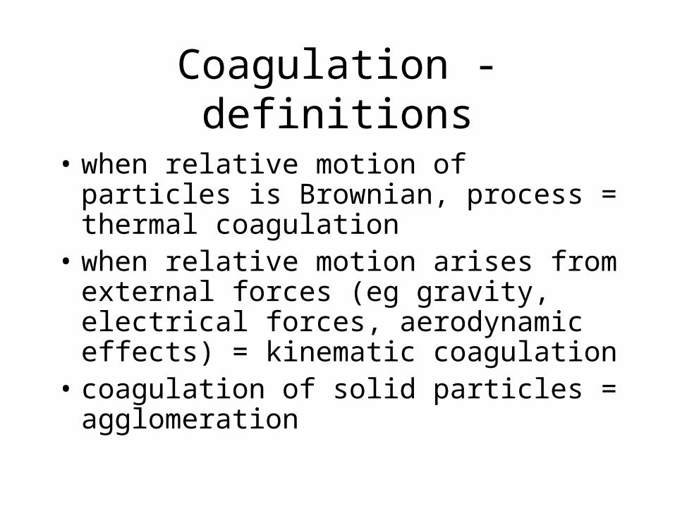
Coagulation - definitions

• when relative motion of particles is Brownian, process = thermal coagulation

• when relative motion arises from external forces (eg gravity, electrical forces, aerodynamic effects) = kinematic coagulation

• coagulation of solid particles = agglomeration

Collision frequency function

collision frequency - # collisions/time between particles of size i and size j = vi, vj are volumes ofparticles of size i and j

€

N ij = β vi ,v j( ) ni,n j

depends on the size of the colliding particles, and properties ofsystem such as temperature and pressure

Consider the change in number concentration of particles of sizek, where vk = vi + vj

Coagulation - discrete distributionsFor a discrete size distribution, the rate of formation of particles of size k by collision of particles of size i and j, is given by: where the factor 1/2 is introduced

because each collision is countedtwice in summation

1

2N iji j k+ =∑

Rate of loss of particles of size k by collision with all other particles is given by: N iki=

∞∑ 1

Change in number concentration of particles of size k given by:

iki,i ikkjiji,kji iji ikkji ijk nvvnnnvvNN

dt

dn)()(

2

1

2

111 ∑∑∑∑ ∞

==+

∞

==+−=−=

theory of coagulation for discrete spectrum developed by Smoluchowski (1917) change = formation - loss

Simple example

Collision frequency functions

€

ij =2kT

3μ

1

v i1/ 3

+1

v j1/ 3

⎛

⎝ ⎜ ⎜

⎞

⎠ ⎟ ⎟ v i

1/ 3 + v j1/ 3

( )

for particles in continuum regime:(Stokes-Einstein relationship valid)

( )π ρij

p i ji j

kT

v vv v=

⎛⎝⎜

⎞⎠⎟

⎛

⎝⎜⎜

⎞

⎠⎟⎟ +

⎛

⎝⎜⎜

⎞

⎠⎟⎟ +

3

4

6 1 11 6 1 2 1 2

1 3 1 32

/ / /

/ /

for particles in free molecular regime: (derived from kinetic theory of collisionsbetween hard spheres)

interpolation formulas between regimes given by Fuchs (1964) The Mechanics of Aerosols

Collision frequency values:

where particle diameters, d1 and d2 are in microns

1010 cm3/secd1/d2 0.01 0.1 1.0

0.01 180.1 240 14.41.0 3200 48 6.8

Coagulation: simple test caseAssume we have a monodisperse population initially, and particle diameter is greater than gas mean free path(continuum regime), so vi = vj

€

ij =2kT

3μ

1

v i1/ 3

+1

v j1/ 3

⎛

⎝ ⎜ ⎜

⎞

⎠ ⎟ ⎟ v i

1/ 3 + v j1/ 3

( ) =8kT

3μ= K

dn

dt

Kn n Kn nk

i j k i j k i i= −+ = =

∞∑ ∑2 1

coagulation equation is then:

let i in N=

∞

∞∑ =1

2

2 - ∞

∞ = NK

dtdNcoagulation equation simplifies to:

Simple test case continued

solving for total number concentration as f(t)

NNKN t∞

∞

∞=

+⎛⎝⎜⎞⎠⎟

( )( )0

10

2

using the boundary condition:N N∞ ∞= =( )0 0 at t

t

N

NKN=

−∞

∞

∞

( )

( )

01

02

solving for time

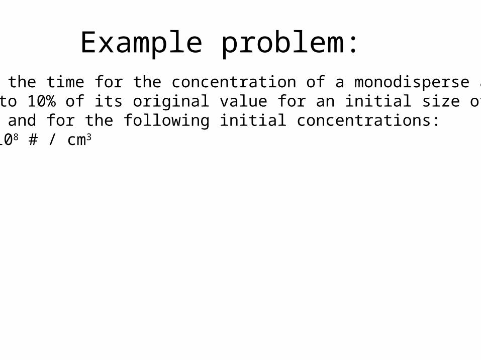
Example problem: Estimate the time for the concentration of a monodisperse aerosolto fall to 10% of its original value for an initial size of dp =1 micron and for the following initial concentrations: 103 and 108 # / cm3

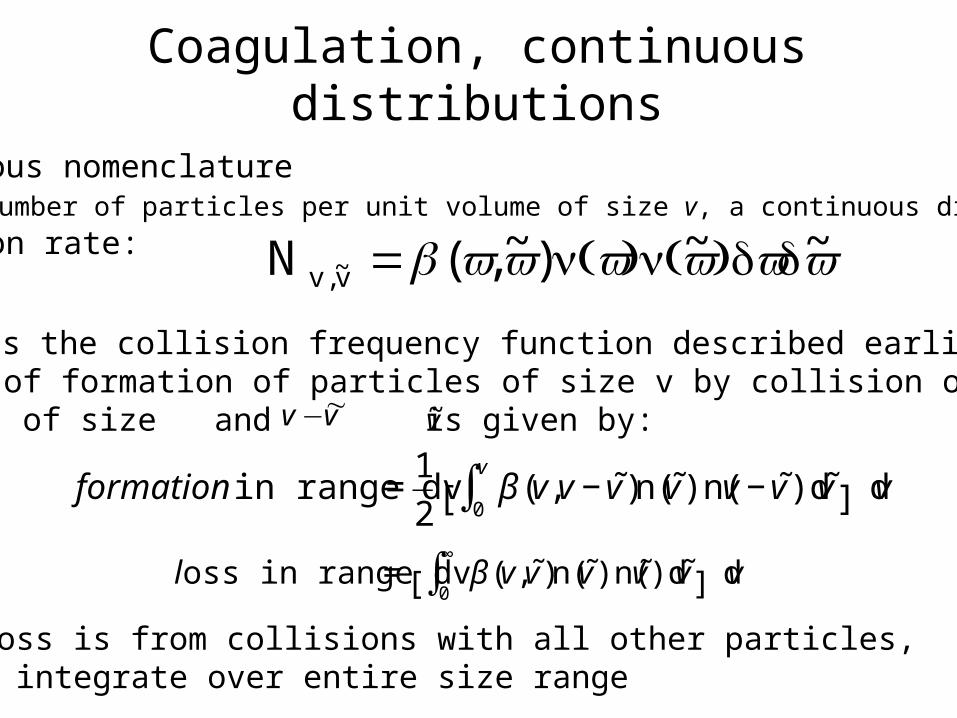
Coagulation, continuous distributions

continuous nomenclature n(v) = number of particles per unit volume of size v, a continuous distribution

collision rate: N v v,~ ( , ~) ~ ~= v v v v v v(n ) (n )d d

where is the collision frequency function described earlierThe rate of formation of particles of size v by collision of smaller particles of size and is given by: v v−~ ~v

€

formation in range dv =1

2 0

v

∫ β (v,v − ˜ v )n( ˜ v )n(v − ˜ v )d ˜ v [ ] dv

€

loss in range dv =0

∞

∫ β (v, ˜ v )n( ˜ v )n( ˜ v )d ˜ v [ ] dv

Here, loss is from collisions with all other particles, so must integrate over entire size range

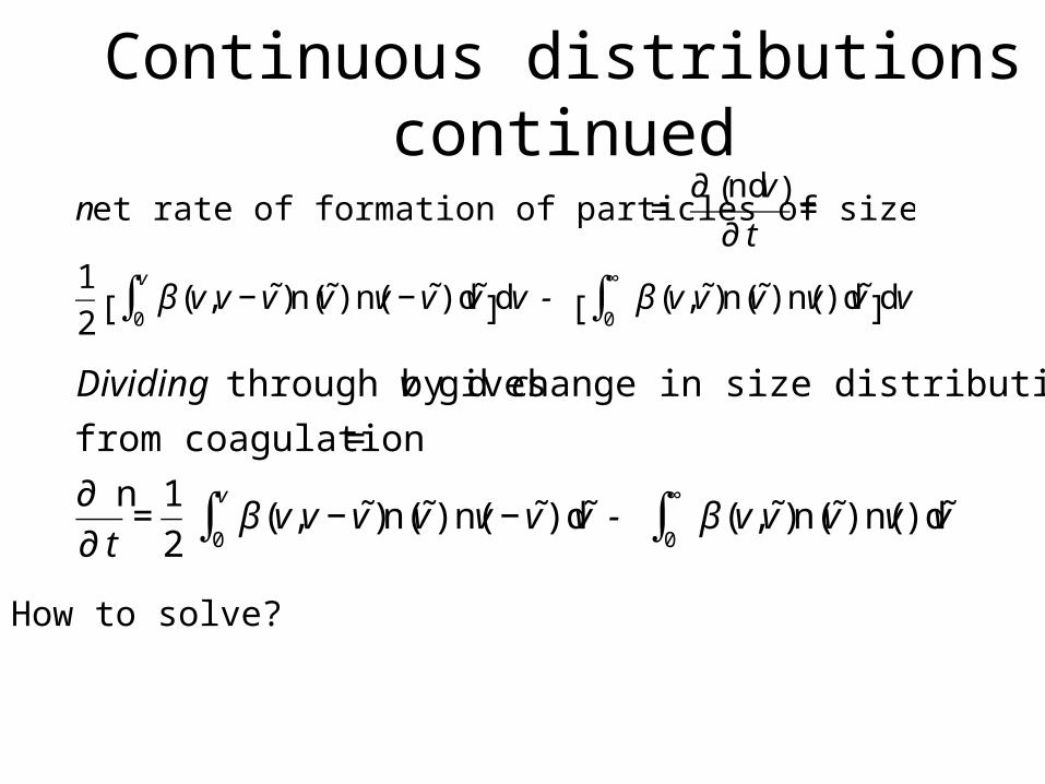
Continuous distributions continued

€

net rate of formation of particles of size v = ∂ ndv( )

∂ t=

1

2 0

v

∫ β (v,v − ˜ v )n( ˜ v )n(v − ˜ v )d ˜ v [ ]dv - 0

∞

∫ β (v, ˜ v )n( ˜ v )n(v)d ˜ v [ ]dv

€

Dividing through by dv gives change in size distribution resulting

from coagulation =

∂ n

∂ t=

1

2 0

v

∫ β (v,v − ˜ v )n( ˜ v )n(v − ˜ v )d ˜ v - 0

∞

∫ β (v, ˜ v )n( ˜ v )n(v)d ˜ v

How to solve?

Recall: similarity transformation

The similarity transformation for the particle size distributionis based on the assumption that the fraction of particles in agiven size range (ndv) is a function only of particle volume normalized by average particle volume:

nd

Nd

v v

v

v

v∞

=⎛⎝⎜

⎞⎠⎟⎛⎝⎜

⎞⎠⎟

ψhere, average particle vo lume =

V

N where V i s total aerosol volume

v

=∞

defining a new variable, and rearranging, η = = ∞v

v

vN

V

n tN

V( , ) ( )v = ∞

2

ψ η

Self-preserving size distribution

For simplest case: no material added or lost from the system,V is constant, but is decreasing as coagulation takes place.N∞

If the form of is known, and if the size distribution corresponding to any value of V and is known forany one time, t, then the size distribution at any other time can bedetermined. In other words, the shapes of the distributions at different times are similar, and can be related using a scalingfactor. These distributions are said to be ‘self-preserving’.

ψ η( )

N∞

ψ η( )

η

t1

t2

t3

Special cases - free molecular regime, coagulation of spheres

• Brownian coagulation in free molecular regime: Lai,

Friedlander, Pich, Hidy, J. Colloid Int. Sci. 39, 395 (1972).

• allows estimation of change in total number concentration resulting from coagulation, if a self-preserving distribution is assumed

• is an integral function of ψ, and is found to be about 6.67

6/116/1

2/16/16

4

3

2 ∞∞

⎟⎟⎠

⎞⎜⎜⎝

⎛⎟⎠

⎞⎜⎝

⎛−= NVkT

dtdN

particleρπ Note V =volume fraction,

vol aerosol / total volume gas plus aerosol

• When primary particles collide and stick, but do not coalesce, irregular structures are formed

agglomerate spherical equivalent

• Recall - we can use a fractal dimension to characterize these structures

Coagulation of hard spheres

v

v

r

ro

D f

=⎛

⎝⎜

⎞

⎠⎟ =

0034

3 where v r is the v olume of t he primary particleo π

Above equation gives: the relationship between radius r (rgyration usually) of aerosol agglomerates, and the volume of primary particles in the agglomerate

Special cases - free molecular growth of fractal agglomerates

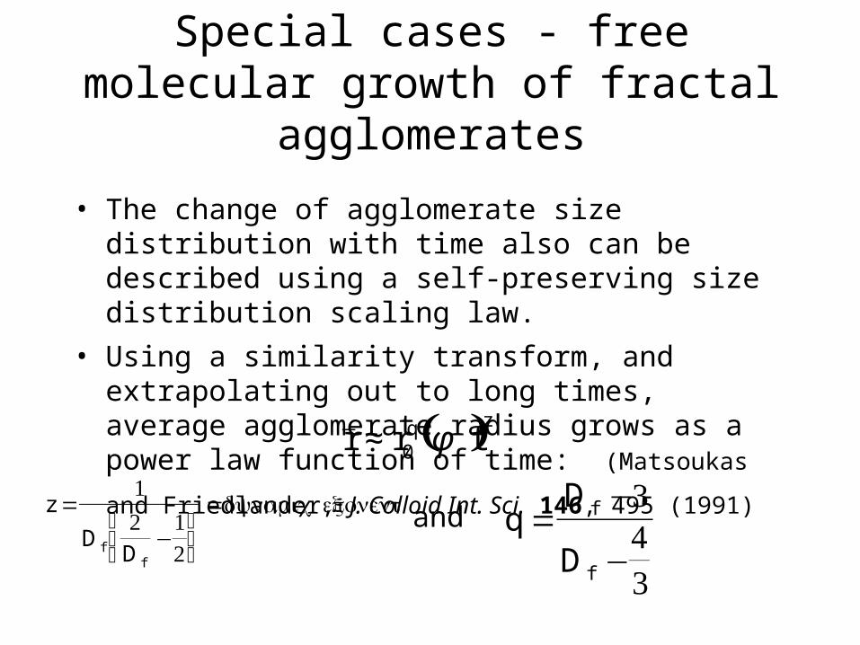
• The change of agglomerate size distribution with time also can be described using a self-preserving size distribution scaling law.

• Using a similarity transform, and extrapolating out to long times, average agglomerate radius grows as a power law function of time: (Matsoukas and Friedlander, J. Colloid Int. Sci.

146, 495 (1991) ( )r r q z≈ 0 φ t

z

DDf

f

=−

⎛

⎝⎜

⎞

⎠⎟

=12 1

2

dynamic exponent and qD

D

f

f

=−

−

343

Interesting result!

• For Df = 3, growth rate is independent of primary particle size.

• But, for Df < 3, then the exponent q is negative

• So smaller primary particles result in larger agglomerates!

Summary of processes affecting suspended particles

• Transport by diffusion and external fields

• Formation by nucleation

• Condensation and evaporation

• Coagulation

Balances: