Co-Training for Domain Adaptation - NIPS

Co-Training for Domain Adaptation

Minmin Chen, Kilian Q. WeinbergerDepartment of Computer Science and Engineering

Washington University in St. LouisSt. Louis, MO 63130

mc15,[email protected]

John C. BlitzerGoogle Research

1600 Amphitheatre ParkwayMountain View, CA [email protected]

Abstract

Domain adaptation algorithms seek to generalize a model trained in a source do-main to a new target domain. In many practical cases, the source and target dis-tributions can differ substantially, and in some cases crucial target features maynot have support in the source domain. In this paper we introduce an algorithmthat bridges the gap between source and target domains by slowly adding to thetraining set both the target features and instances in which the current algorithmis the most confident. Our algorithm is a variant of co-training [7], and we nameit CODA (Co-training for domain adaptation). Unlike the original co-trainingwork, we do not assume a particular feature split. Instead, for each iteration of co-training, we formulate a single optimization problem which simultaneously learnsa target predictor, a split of the feature space into views, and a subset of source andtarget features to include in the predictor. CODA significantly out-performs thestate-of-the-art on the 12-domain benchmark data set of Blitzer et al. [4]. Indeed,over a wide range (65 of 84 comparisons) of target supervision CODA achievesthe best performance.

1 Introduction

Domain adaptation addresses the problem of generalizing from a source distribution for whichwe have ample labeled training data to a target distribution for which we have little or no la-bels [3, 14, 28]. Domain adaptation is of practical importance in many areas of applied machinelearning, ranging from computational biology [17] to natural language processing [11, 19] to com-puter vision [23].

In this work, we focus primarily on domain adaptation problems that are characterized by missingfeatures. This is often the case in natural language processing, where different genres often usevery different vocabulary to describe similar concepts. For example, in our experiments we use thesentiment data of Blitzer et al. [4], where a breeze to use is a way to express positive sentiment aboutkitchen appliances, but not about books. In this situation, most domain adaptation algorithms seekto eliminate the difference between source and target distributions, either by re-weighting sourceinstances [14, 18] or learning a new feature representation [6, 28].

We present an algorithm which differs from both of these approaches. Our method seeks to slowlyadapt its training set from the source to the target domain, using ideas from co-training. We accom-plish this in two ways: First, we train on our own output in rounds, where at each round, we includein our training data the target instances we are most confident of. Second, we select a subset ofshared source and target features based on their compatibility. Different from most previous workon selecting features for domain adaptation, the compatibility is measured across the training setand the unlabeled set, instead of across the two domains. As more target instances are added to thetraining set, target specific features become compatible across the two sets, therefore are includedin the predictor. Finally, we exploit the pseudo multiview co-training algorithm of Chen et al. [10]

1

to exploit the unlabeled data efficiently. These three intuitive ideas can be combined in a singleoptimization problem. We name our algorithm CODA (Co-Training for Domain Adaptation).

By allowing us to slowly change our training data from source to target, CODA has an advantageover representation-learning algorithms [6, 28], since they must decide a priori what the best repre-sentation is. In contrast, each iteration of CODA can choose exactly those few target features whichcan be related to the current (source and pseudo-labeled target) training set. We find that in thesentiment prediction data set of Blitzer et al. [4] CODA improves the state-of-the-art cross widelyvarying amounts of target labeled data in 65 out of 84 settings.

2 Notation and Setting

We assume our data originates from two domains, Source (S) and Target (T). The source datais fully labeled DS = {(x1, y1), . . . , (xns

, yns)} ⊂ Rd × Y and sampled from some distribu-

tion PS(X,Y ). The target data is sampled from PT (X,Y ) and is divided into labeled DlT =

{(x1, y1), . . . , (xnt , ynt)} ⊂ Rd×Y and unlabeled DuT = {(x1, ?), . . . (xmt , ?)} ⊂ Rd×Y parts,

where in the latter the labels are unknown during training time. Both domains are of equal dimen-sionality d. Our goal is to learn a classifier h ∈ H to accurately predict the labels on the unlabeledportion of DT , but also to extend to out-of-sample test points, such that for any (x, y) sampledfrom PT , we have h(x) = y with high probability. For simplicity we assume that Y = {+1,−1},although our method can easily be adapted to multi-class or regression settings.

We assume the existence of a base classifier, which determines the setH. Throughout this paper wesimply use logistic regression, i.e. our classifier is parameterized by a weight-vector w ∈ Rd anddefined as hw(x) = (1 + e−w

>x)−1. The weights w are set to minimize the loss function

`(w;D) = − 1

|D|∑

(x,y)∈D

log(1 + exp(−yw>x)). (1)

If trained on data sampled from PS(X,Y ), logistic regression models the distribution PS(Y |X) [13]through Ph(Y = y|X = x;w) = (1 + e−w

>xy)−1. In this paper, our goal is to adapt this classifierto the target distribution PT (Y |X).

3 Method

In this section, we begin with a semi-supervised approach and describe the rote-learning procedure toautomatically annotate target domain inputs. The algorithm maintains and grows a training set that isiteratively adapted to the target domain. We then incorporate feature selection into the optimization,a crucial element of our domain-adaptation algorithm. The feature selection addresses the change indistribution and support from PS to PT . Further, we introduce pseudo multi-view co-training [7, 10],which improves the rote-learning procedure by adding inputs with features that are still not usedeffectively by the current classifier. We use automated feature decomposition to artificially split ourdata into multiple views, explicitly to enable successful co-training.

3.1 Self-training for Domain Adaptation

First, we assume we are given a loss function ` – in our case the log-loss from eq. (1) – whichprovides some estimate of confidence in its predictions. In logistic regression, if y = sign(h(x)) isthe prediction for an input x, the probability Ph(Y = y|X = x;w) is a natural metric of certainty(as h(x) can be interpreted as a probability for x to be of label +1), but other methods [22] canbe used. Self-training [19] is a simple and intuitive iterative algorithm to leverage unlabeled data.During training one maintains a labeled training set L and an unlabeled test set U , initialized asL = DS ∪Dl

T and U = DuT . Each iteration, a classifier hw is trained to minimize the loss function

` over L and is evaluated on all elements of U . The c most confident predictions on U are moved toL for the next iteration, labeled by the prediction of sign(hw). The algorithm terminates when U isempty or all predictions are below a pre-defined confidence threshold (and considered unreliable).Algorithm 1 summarizes self-training in pseudo-code with the use of feature selection, described inthe following section.

2

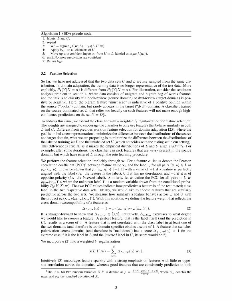
Algorithm 1 SEDA pseudo-code.1: Inputs: L and U .2: repeat3: w∗ = argminw`(w;L) + γs(L,U,w)4: Apply hw∗ on all elements of U .5: Move up-to c confident inputs xi from U to L, labeled as sign(h(xi)).6: until No more predictions are confident7: Return hw∗

3.2 Feature Selection

So far, we have not addressed that the two data sets U and L are not sampled from the same dis-tribution. In domain adaptation, the training data is no longer representative of the test data. Moreexplicitly, PS(Y |X = x) is different from PT (Y |X = x). For illustration, consider the sentimentanalysis problem in section 4, where data consists of unigram and bigram bag-of-words featuresand the task is to classify if a book-review (source domain) or dvd-review (target domain) is pos-itive or negative. Here, the bigram feature “must read” is indicative of a positive opinion withinthe source (“books”) domain, but rarely appears in the target (“dvd”) domain. A classifier, trainedon the source-dominated set L, that relies too heavily on such features will not make enough high-confidence predictions on the set U = Du

T .

To address this issue, we extend the classifier with a weighted `1 regularization for feature selection.The weights are assigned to encourage the classifier to only use features that behave similarly in bothL and U . Different from previous work on feature selection for domain adaptation [25], where thegoal is to find a new representation to minimize the difference between the distributions of the sourceand target domain, what we are proposing is to minimize the difference between the distributions ofthe labeled training setL and the unlabeled setU (which coincides with the testing set in our setting).This difference is crucial, as it makes the empirical distributions of L and U align gradually. Forexample, after some iterations, the classifier can pick features that are never present in the sourcedomain, but which have entered L through the rote-learning procedure.

We perform the feature selection implicitly through w. For a feature α, let us denote the Pearsoncorrelation coefficient (PCC)1 between feature value xα and the label y for all pairs (x, y) ∈ L asρL(xα, y). It can be shown that ρL(xα, y) ∈ [−1, 1] with a value of +1 if a feature is perfectlyaligned with the label (i.e. the feature is the label), 0 if it has no correlation, and −1 if it is ofopposite polarity (i.e. the inverted label). Similarly, let us define the PCC for all pairs in U asρU ;w(xα, Y ), where the unknown label Y is a random variable drawn from the conditional proba-bility Ph(Y |X;w). The two PCC values indicate how predictive a feature is of the (estimated) classlabel in the two respective data sets. Ideally, we would like to choose features that are similarlypredictive across the two sets. We measure how similarly a feature behaves across L and U withthe product ρL(xα, y)ρU ;w(xα, Y ). With this notation, we define the feature weight that reflects thecross-domain incompatibility of a feature as

∆L,U,w(α) = (1− ρL(xα, y)ρU ;w(xα, Y )). (2)

It is straight-forward to show that ∆L,U,w ∈ [0, 2]. Intuitively, ∆L,U,w expresses to what degreewe would like to remove a feature. A perfect feature, that is the label itself (and the prediction inU ), results in a score of 0. A feature that is not correlated with the class label in at least one ofthe two domains (and therefore is too domain-specific) obtains a score of 1. A feature that switchespolarization across domains (and therefore is “malicious”) has a score ∆L,U,w(α) > 1 (in theextreme case if it is the label in L and the inverted label in U , its score would be 2).

We incorporate (2) into a weighted `1 regularization

s(L,U,w) =

d∑α=1

∆L,U,w(α)|wα|. (3)

Intuitively (3) encourages feature sparsity with a strong emphasis on features with little or oppo-site correlation across the domains, whereas good features that are consistently predictive in both

1The PCC for two random variables X,Y is defined as ρ = E[(X−µX )(Y−µY )]σXσY

, where µX denotes themean and σX the standard deviation of X .

3

domains become cheap. We refer to this version of the algorithm as Self-training for Domain Adap-tation (SEDA). The optimization with feature selection, used in Algorithm 1, becomes

w = argminw`(L) + γs(L,U,w). (4)

Here, γ ≥ 0 denotes the loss-regularization trade-off parameter. As we have very few labeled inputsfrom the target domain in the early iterations, stronger regularization is imposed so that only featuresshared across the two domains are used. When more and more inputs from the target domain areincluded in the training set, we gradually decrease the regularization to accommodate target specificfeatures. The algorithm is very insensitive to the exact initial choice of γ. The guideline is to startwith a relatively large number, and decrease it until the selected feature set is not empty. In ourimplementation, we set it to γ0 = 0.1, and we divide it by a factor of 1.1 during each iteration.

3.3 Co-training for Domain Adaptation

For rote-learning to be effective, we need to move test inputs from U to L that 1) are correctlyclassified (with high probability) and 2) have potential to improve the classifier in future iterations.The former is addressed by the feature selecting regularization from the previous section – restrictingthe classifier to a sub-set of features that are known to be cross-data set compatible reduces thegeneralization error on U . In this section we address the second requirement. We want to add inputsxi that contain additional features, which were not used to obtain the prediction hw(xi) and wouldenrich the training set L.

If the exact labels of the inputs in U were known, a good active learning [26] strategy would be tomove inputs to L on which the current classifier hw is most uncertain. In our setting, this wouldbe clearly ill advised as the uncertain prediction is also used as the label. A natural solution to thisdilemma is co-training [7]. Co-training assumes the data set is presented in two separate views andtwo classifiers are trained, one in each view. Each iteration, only inputs that are confident accordingto exactly one of the two classifiers are moved to the training set. This way, one classifier providesthe (estimated) labels to the inputs on which the other classifier is uncertain.

In our setting we do not have multiple views and which features are selected varies in each iteration.Hence, co-training does not apply out-of-the-box. We can, however, split our features into two mu-tually exclusive views such that co-training is effective. To this end we follow the pseudo-multiviewregularization introduced by Chen et al. [10]. The main intuition is to train two classifiers on a singleview X such that: (1) both perform well on the labeled data; (2) both are trained on strictly differentfeatures; (3) together they are likely to satisfy Balcan’s condition of ε-expandability [2], a necessaryand sufficient pre-condition for co-training to work2. These three aspects can be formulated explic-itly as three modifications of our optimization problem (4). We discuss each of them in detail in thefollowing.

Loss. Two classifiers are required for co-training, whose weight vectors we denote by u and v. Theperformance of each classifier is measured by the log-loss `(·;L) in eq. (1). To ensure that bothclassifiers perform well on the training set L, i.e. both have a small training loss, we train themjointly while minimizing the soft-maximum3 of the two losses,

log(e`(u;L) + e`(v;L)

). (5)

Feature Decomposition. Co-training requires the two classifiers to be trained on different featurespaces. We create those by splitting the feature-space into two mutually exclusive sub-sets. Moreprecisely, for each feature α, at least one of the two classifiers must have a zero weight in the αthdimension. We can enforce this across all features with the equality constraint

d∑α=1

u2αv

2α = 0. (6)

ε-Expandability. In the original co-training formulation [7], it is assumed that the two views ofthe data are class conditionally independent. This assumption is very strong and can easily be

2Provided that the classifiers are never confident and wrong — which can be violated in practice.3The soft-max of a set of elements S is a differentiable approximation of max(S) ≈ log(

∑s∈S e

s).

4

violated in practice [20]. Recent work [2] weakens this requirement significantly to a condition ofε-expandability. Loosely phrased, for the two classifiers to be able to teach each other, they mustmake confident predictions on different subsets of the unlabeled set U .

For the classifier hu, let y = sign(u>x) ∈ {±1} denote the class prediction and Ph(y|x;u) itsconfidence. Define cu(x) as a confidence indicator function (for some confidence threshold τ > 0)4

cu(x) =

{1 if p(y|x;u) > τ0 otherwise, (7)

and cv respectively. Then the ε-expanding condition translates to

∑x∈U

[cu(x)cv(x) + cu(x)cv(x)] ≥ εmin

[∑x∈U

cu(x)cv(x),∑x∈U

cu(x)cv(x)

], (8)

for some ε > 0. Here, cu(x) = 1− cu(x) indicates that classifier hu is not confident about input x.Intuitively, the constraint in eq. (8) ensures that the total number of inputs in U that can be used forrote-learning because exactly one classifier is confident (LHS), is larger than the set of inputs whichcannot be used because both classifiers are already confident or both are not confident (RHS).

In summary, the framework splits the feature space into two mutually exclusive sub-sets. This rep-resentation enables us to train two logistic regression classifiers, both with small loss on the labeleddata set, while satisfying two constraints to ensure feature decomposition and ε-expandability. Ourfinal classifier has the weight vector w = u + v. We refer to the resulting algorithm as CODA (Co-training for Domain Adaptation), which can be stated concisely with the following optimizationproblem:

minw,u,v

log(e`(u;L) + e`(v;L)

)+ γs(L,U,w)

subject to:(1)∑di=1 u

2iv

2i = 0

(2)∑

x∈U [cu(x)cv(x) + cu(x)cv(x)] ≥ εmin[∑

x∈U cu(x)cv(x),∑

x∈U cu(x)cv(x)]

(3) w = u + v

The optimization is non-convex. However, as it is not particularly sensitive to initialization, we setu,v randomly and optimize with standard conjugate gradient descent5. Due to space constraints wedo not include a pseudo-code implementation of CODA. The implementation is essentially identicalto that of SEDA (Algorithm 1) where the above optimization problem is solved instead of eq. (4) inline 3. In line 5, we move inputs that one classifier is confident about while the other one is uncertainto the training set L to improve the classifier in future iterations.

4 Results

We evaluate our algorithm together with several other domain adaptation algorithms on the “Amazonreviews” benchmark data sets [6]. The data set contains reviews of four different types of products:books, DVDs, electronics, and kitchen appliances from Amazon.com. In the original dataset, eachreview is associated with a rating of 1-5 stars. For simplicity, we are only concerned about whetheror not a review is positive (higher than 3 stars) or negative (3 stars or lower). That is, yi = {+1,−1},where yi = 1 indicates that it is a positive review, and −1 otherwise. The data from four domainsresults in 12 directed adaptation tasks (e.g. books → dvds). Each domain adaptation task consistsof 2, 000 labeled source inputs and around 4, 000 unlabeled target test inputs (varying slightly be-tween tasks). We let the amount of labeled target data vary from 0 to 1600. For each setting withtarget labels we ran 10 experiments with different, randomly chosen, labeled instances. The origi-nal feature space of unigrams and bigrams is on average approximately 100, 000 dimensions across

4In our implementation, the 0-1 indicator was replaced by a very steep differentiable sigmoid function, andτ was set to 0.8 across different experiments.

5We use minimize.m (http://tinyurl.com/minimize-m).

5

different domains. To reduce the dimensionality, we only use features that appear at least 10 timesin a particular domain adaptation task (with approximately 40, 000 features remaining). Further, wepre-process the data set with standard tf-idf [24] feature re-weighting.

0 50 100 200 400 800 16000.7

0.75

0.8

0.85

0.9

0.95

1

1.05

Rel

ativ

e Te

st E

rror

Number of target labeled data

Logistic RegressionSelf−trainingSEDACODA

0 50 100 200 400 800 16000.75

0.8

0.85

0.9

0.95

1

1.05

1.1

1.15

Rela

tive

Test

Erro

r


Logistic RegressionCoupledEasyAdaptEasyAdapt++CODA

Figure 1: Relative test-error reduction over logistic regression, averaged across all 12 domain adap-tation tasks, as a function of the target training set size. Left: A comparison of the three algorithmsfrom section 3. The graph shows clearly that self-training (Self-training vs. Logistic Regression),feature-selection (SEDA vs. Self-training) and co-training (CODA vs. SEDA), each improve theaccuracy substantially. Right: A comparison of CODA with four state-of-the-art domain adaptationalgorithms. CODA leads to particularly strong improvements under little target supervision.

As a first experiment, we compare the three algorithms from Section 3 and logistic regression as abaseline. The results are in the left plot of figure 1. For logistic regression, we ignore the differencebetween source and target distribution, and train a classifier on the union of both labeled data sets.We use `2 regularization, and set the regularization constant with 5-fold cross-validation. In figure 1,all classification errors are shown relative to this baseline. Our second baseline is self-training,which adds self-training to logistic regression – as described in section 3.1. We start with the setof labeled instances from source and target domain, and gradually add confident predictions to thetraining set from the unlabeled target domain (without regularization). SEDA adds feature selectionto the self-training procedure, as described in section 3.2. We optimize over 100 iterations of self-training, at which stage the regularization was effectively zero and the classifier converged. ForCODA we replace self-training with pseudo-multi-view co-training, as described in section 3.3.

The left plot in figure 1 shows the relative classification errors of these four algorithms averaged overall 12 domain adaptation tasks, under varying amounts of target labels. We observe two trends: First,there are clear gaps between logistic regression, self-training, SEDA, and CODA. From these threegaps one can conclude that self-training, feature-selection and co-training each lead to substantialimprovements in classification error. A second trend is that the relative improvement over logisticregression reduces as more labeled target data becomes available. This is not surprising, as withsufficient target labels the task turns into a classical supervised learning problem and the source databecomes irrelevant.

As a second experiment, we compare CODA against three state-of-the-art domain adaptation algo-rithms. We refer to these as Coupled, the coupled-subspaces approach [6], EasyAdapt [11], andEasyAdapt++. [15]. Details about the respective algorithms are provided in section 5. Coupledsubspaces, as described in [6], does not utilize labeled target data and its result is depicted as asingle point. The right plot in figure 1 compares these algorithms, relative to logistic regression.Figure 3 shows the individual results on all the 12 adaptation tasks with absolute classification errorrates. The error bars show the standard deviation across the 10 runs with different labeled instances.EasyAdapt and EasyAdapt++, both consistently improve over logistic regression once sufficient tar-get data is available. It is noteworthy that, on average, CODA outperforms the other algorithmsin almost all settings when 800 labeled target points or less are present. With 1600 labeled targetpoints all algorithms perform similar to the baseline and additional source data is irrelevant. Allhyper-parameters of competing algorithms were carefully set by 5-fold cross validation.

Concerning computational requirements, it is fair to say that CODA is significantly slower than theother algorithms, as each iteration is of comparable complexity as logistic regression or EasyAdapt.

6

20 40 60 80 1000.9

1

1.1

1.2

1.3

1.4

Iterations

Rat

io o

f use

d fe

atur

es

Source heavy

Target heavy

20 40 60 80 1000.9

1

1.1

1.2

1.3

1.4

Iterations

Rat

io o

f use

d fe

atur

es

20 40 60 80 1000.9

1

1.1

1.2

1.3

1.4

Iterations

Rat

io o

f use

d fe

atur

es

Source heavy

Target heavy

Source heavy

Target heavy

0 target labels 400 target labels 1600 target labels

Rat

io o

f use

d fe

atur

es (s

ourc

e/ta

rget

)

r(w)

Ratio of used features (source/target)

Figure 2: The ratio of the average number of used features between source and target inputs (9),tracked throughout the CODA optimization. The three plots show the same statistic at differentamounts of target labels. Initially, an input from the source domain has on average 10-35% morefeatures that are used by the classifier than a target input. At around iteration 40, this relation changesand the classifier uses more target-typical features. The graph shows the geometric mean across alladaptation tasks. With no target data available (left plot), the early spike in source dominance ismore pronounced and decreases when more target labels are available (middle and right plot).

In typical domain adaptation settings this is generally not a problem, as training sets tend to be small.In our experiments, the average training time for CODA6 was about 20 minutes.

Finally, we investigate the feature-selection process during CODA training. Let us define the indi-cator function δ(a) ∈ {0, 1} to be δ(a) = 0 if and only if a = 0, which operates element-wise onvectors. The vector δ(w) ∈ {0, 1}d indicates which features are used in the classifier and δ(xi) in-dicates which features are present in input xi. We can denote the ratio between the average numberof used features in labeled training inputs over those in unlabeled target inputs as

r(w) =

1|Dl

S|∑

xs∈DlSδ(w)>δ(xs)

1|Dl

T|∑

xt∈DlTδ(w)>δ(xt)

. (9)

Figure 2 shows the plot of r(w) for all weight vectors during the 100 iterations of CODA, averagedacross all 12 data sets. The three plots show the same statistic under varying amounts of targetlabels. Two trends can be observed: First, during CODA training, the classifier initially selectsmore source-specific features. For example in the case with zero labeled target data, during earlyiterations the average source input contains 20 − 35% more used features relative to target inputs.This source-heavy feature distribution changes and eventually turns into target-heavy distribution asthe classifier adapts to the target domain. As a second trend, we observe that with more target labels(right plot), this spike in source features is much less pronounced whereas the final target-heavyratio is unchanged but starts earlier. This indicates that as the target labels increase, the classifiermakes less use of the source data and relies sooner and more directly on the target signal.

5 Related Work and Discussion

Domain adaptation algorithms that do not use labeled target domain data are sometimes called un-supervised adaptation algorithms. There are roughly three types of algorithms in this group. Thefirst type, which includes the coupled subspaces algorithm of Blitzer et al. [5], learns a shared rep-resentation under which the source and target distributions are closer than under the ambient featurespace [28]. The largest disadvantage of these algorithms is that they do not jointly optimize thepredictor and the representation, which prevents them from focusing on those features which areboth different and predictive. By jointly optimizing the feature selection, the multi-view split andthe prediction, CODA allows us to do both.

The second type of algorithm attempts to directly minimize the divergence between domains, typ-ically by weighting individual instances [14, 16, 18]. These algorithms do not assume highly di-vergent domains (e.g. those with unique target features), but they have the advantage over bothCODA and representation-learning of learning asymptotically optimal target predictors from only

6We used a straight-forward MatlabTM implementation.

7

0 50 100 200 400 800 16000.1

0.15

0.2

0.25

0.3

0.35

Test

Erro

r

Dvd −> Books



0 50 100 200 400 800 16000.1

0.15

0.2

0.25

0.3

0.35

Test

Erro

r

Electronics −> Books



0 50 100 200 400 800 16000.1

0.15

0.2

0.25

0.3

0.35

Test

Erro

r

Kitchen −> Books



0 50 100 200 400 800 16000.1

0.15

0.2

0.25

0.3

0.35

Test

Erro

r

Books −> Dvd



0 50 100 200 400 800 1600

0.2

0.25

0.3

0.35

Test

Erro

r

Electronics −> Dvd



0 50 100 200 400 800 16000.1

0.15

0.2

0.25

0.3

0.35

Test

Erro

r

Kitchen −> Dvd



0 50 100 200 400 800 16000.1

0.15

0.2

0.25

0.3

0.35

Test

Erro

r

Books −> Electronics



0 50 100 200 400 800 16000.1

0.15

0.2

0.25

0.3

0.35

Test

Erro

r

Dvd −> Electronics



0 50 100 200 400 800 16000.05

0.1

0.15

0.2

0.25

0.3

Test

Erro

r

Kitchen −> Electronics



0 50 100 200 400 800 16000.1

0.15

0.2

0.25

0.3

0.35

Test

Erro

r

Books −> Kitchen



0 50 100 200 400 800 16000.1

0.15

0.2

0.25

Test

Err

or

Dvd −> Kitchen



0 50 100 200 400 800 16000.08

0.1

0.12

0.14

0.16

0.18

Test

Erro

rElectronics −> Kitchen



Figure 3: The individual results on all domain adaptation tasks under varying amounts of labeledtarget data. The graphs show the absolute classification error rates. All settings with existing labeledtarget data were averaged over 10 runs (with randomly selected labeled instances). The vertical barsindicate the standard deviation in these cases.

source training data (when their assumptions hold). We did not explore them here because theirassumptions are clearly violated for this data set.

In natural language processing, a final type of very successful algorithm self-trains on its own targetpredictions to automatically annotate new target domain features [19]. These methods are mostclosely related, in spirit, to our own CODA algorithm. Indeed, our self-training baseline is intendedto mimic this style of algorithm.

The final set of domain adaptation algorithms, which we compared against but did not describe, arethose which actively seek to minimize the labeling divergence between domains using multi-tasktechniques [1, 8, 9, 12, 21, 27]. Most prominently, Daume [11] trains separate source and targetmodels, but regularizes these models to be close to one another. The EasyAdapt++ variant of thisalgorithm, which we compared against, generalizes this to the semi-supervised setting by making theassumption that for unlabeled target instances, the tasks should be similar. Although these methodsdid not significantly out-perform our baselines in the sentiment data set, we note that there do existdata sets on which such multi-task techniques are especially important [11], and we hope soon toexplore combinations of CODA with multi-task learning on those data sets.

8

References[1] R.K. Ando and T. Zhang. A framework for learning predictive structures from multiple tasks and unla-

beled data. The Journal of Machine Learning Research, 6:1817–1853, 2005.[2] M.F. Balcan, A. Blum, and K. Yang. Co-training and expansion: Towards bridging theory and practice.

NIPS, 17:89–96, 2004.[3] S. Ben-David, J. Blitzer, K. Crammer, A. Kulesza, F. Pereira, and Jenn Wortman. A theory of learning

from different domains. Machine Learning, 2009.[4] J. Blitzer, M. Dredze, and F. Pereira. Biographies, bollywood, boom-boxes and blenders: Domain adapta-

tion for sentiment classification. In Association for Computational Linguistics, Prague, Czech Republic,2007.

[5] J. Blitzer, D. Foster, and S. Kakade. Domain adaptation with coupled subspaces. In Conference onArtificial Intelligence and Statistics, Fort Lauterdale, 2011.

[6] J. Blitzer, R. McDonald, and F. Pereira. Domain adaptation with structural correspondence learning.In Proceedings of the 2006 Conference on Empirical Methods in Natural Language Processing, pages120–128. Association for Computational Linguistics, 2006.

[7] A. Blum and T. Mitchell. Combining labeled and unlabeled data with co-training. In Proceedings of theeleventh annual conference on Computational learning theory, page 100. ACM, 1998.

[8] R. Caruana. Multitask learning. Machine Learning, 28:41–75, 1997.[9] O. Chapelle, P. Shivaswamy, S. Vadrevu, K.Q. Weinberger, Y. Zhang, and B. Tseng. Multi-task learning

for boosting with application to web search ranking. In Proceedings of the 16th ACM SIGKDD interna-tional conference on Knowledge discovery and data mining, KDD ’10, pages 1189–1198, New York, NY,USA, 2010. ACM.

[10] M. Chen, K.Q. Weinberger, and Y. Chen. Automatic Feature Decomposition for Single View Co-training.In International Conference on Machine Learning, 2011.

[11] H. Daume III. Frustratingly easy domain adaptation. In Association for Computational Linguistics, 2007.[12] T. Evgeniou, C.A. Micchelli, and M. Pontil. Learning multiple tasks with kernel methods. Journal of

Machine Learning Research, 6(1):615, 2006.[13] T. Hastie, R. Tibshirani, and J. Friedman. The Elements of Statistical Learning. Springer Verlag, New

York, 2009.[14] J. Huang, A.J. Smola, A. Gretton, K. M. Borgwardt, and B. Scholkopf. Correcting sample selection bias

by unlabeled data. In NIPS 19, pages 601–608. MIT Press, Cambridge, MA, 2007.[15] H. Daume III, A. Kumar, and A. Saha. Co-regularization based semi-supervised domain adaptation. In

NIPS 23, pages 478–486. MIT Press, 2010.[16] J. Jiang and C.X. Zhai. Instance weighting for domain adaptation in nlp. In Proceedings of the 45th Annual

Meeting of the Association of Computational Linguistics, pages 264–271, Prague, Czech Republic, June2007. Association for Computational Linguistics.

[17] Qian Liu, Aaron Mackey, David Roos, and Fernando Pereira. Evigan: a hidden variable model forintegrating gene evidence for eukaryotic gene prediction. Bioinformatics, 2008.

[18] T. Mansour, M. Mohri, and A. Rostamizadeh. Domain adaptation with multiple sources. In NIPS 21,pages 1041–1048. MIT Press, 2009.

[19] D. McClosky, E. Charniak, and M. Johnson. Reranking and self-training for parser adaptation. In Pro-ceedings of the 21st International Conference on Computational Linguistics and the 44th annual meetingof the Association for Computational Linguistics, pages 337–344. Association for Computational Lin-guistics, 2006.

[20] K. Nigam and R. Ghani. Analyzing the effectiveness and applicability of co-training. In Proceedingsof the ninth international conference on Information and knowledge management, pages 86–93. ACM,2000.

[21] S. Parameswaran and K.Q. Weinberger. Large margin multi-task metric learning. In NIPS 23, pages1867–1875. 2010.

[22] J.C. Platt et al. Probabilities for sv machines. NIPS, pages 61–74, 1999.[23] K. Saenko, B. Kulis, M. Fritz, and T. Darrell. Adapting visual category models to new domains. Computer

Vision–ECCV 2010, pages 213–226, 2010.[24] G. Salton and C. Buckley. Term-weighting approaches in automatic text retrieval. Information processing

& management, 24(5):513–523, 1988.[25] S. Satpal and S. Sarawagi. Domain adaptation of conditional probability models via feature subsetting.

Knowledge Discovery in Databases: PKDD 2007, pages 224–235, 2007.[26] B. Settles. Active learning literature survey. Machine Learning, 15(2):201–221, 1994.[27] K.Q. Weinberger, A. Dasgupta, J. Langford, A. Smola, and J. Attenberg. Feature hashing for large scale

multitask learning. In Proceedings of the 26th Annual International Conference on Machine Learning,pages 1113–1120. ACM, 2009.

[28] G. Xue, W. Dai, Q. Yang, and Y. Yu. Topic-bridged plsa for cross-domain text classication. In SIGIR,2008.

9

Co-Training for Domain Adaptation - NIPS

Documents

Transcript of Co-Training for Domain Adaptation - NIPS