Co-Benefits and Additionality of the CleanDevelopment Mechanism: An Empirical Analysis∗

Junjie Zhang†

UC San DiegoCan Wang‡

Tsinghua University

March 22, 2011

Abstract

The Clean Development Mechanism (CDM) allows industrialized countries to com-ply with the Kyoto Protocol by using carbon offsets from developing countries. Thereare two puzzles within this carbon market: additionality (the proposed activity wouldnot have occurred in its absence) and co-benefits (the project has other environmentalbenefits besides climate mitigation). This paper proposes an econometric approach toevaluate the CDM effect on sulfur dioxide emission reductions and assess its addition-ality indirectly. Our empirical model is applied to China’s emissions at the prefecturelevel. We found that the CDM does not have a statistically significant effect in lower-ing sulfur dioxide emissions. This result casts doubt on additionality of these CDMactivities, that is, they would have happened anyway.

Keywords: Clean Development Mechanism, co-benefits, additionality, semipara-metric panel data model.

JEL Classification Numbers: Q54 C23 C14.

∗Junjie Zhang thanks the Center on Emerging and Pacific Economies at UCSD for partial financial sup-port. Can Wang thanks China’s National Science and Technology Pillar Program in the Eleventh Five-YearPlan Period for financial support under grant 2007BAC03A04. We thank Richard Carson, Jason Fleming,Mark Jacobsen, Craig McIntosh, Bruce Mizrach, and David Victor for helpful comments. Suggestions fromthe editor, Dan Phaneuf, and two anonymous referees substantially improved the paper. Our paper alsobenefited from the comments of seminar participants of UCSD Economics Department, IR/PS, TsinghuaUniversity, and ASSA Meetings. Weshi Zhang provided excellent research assistance. Of course, all re-maining errors are ours.†Corresponding author. School of International Relations & Pacific Studies, University of California,

San Diego. 9500 Gilman Drive #0519, La Jolla, CA 92093-0519. Tel: (858) 822-5733. Fax: (858) 534-3939.junjiezhang@ucsd.edu.‡Department of Environmental Science & Engineering, Tsinghua University.

1 Introduction

The Clean Development Mechanism (CDM) is a project-based carbon market which en-

ables industrialized countries to reduce costs of compliance with the Kyoto Protocol by

implementing climate mitigation projects in developing countries. The CDM has been

successful in mobilizing the investment of public and private sectors from both devel-

oped and developing countries for reducing greenhouse gas (GHG) emissions. By the

year 2009, there were more than 4,200 projects in the pipeline that are expected to re-

duce GHG emissions by more than 2,900 million metric tons of carbon dioxide equivalent

(CO2e) by the end of 2012. The CDM emission reduction is not trivial, in that it is around

40 percent of the U.S. emissions in 2007.1

The CDM is nonetheless facing mounting criticism, in which the most serious chal-

lenge is its environmental integrity (Wara, 2007; Victor, 2009; Jaffe, Ranson, and Stavins,

2010). Since there are no emission caps for developing countries, the usefulness of the

CDM hinges on whether the proposed project would have occurred in its absence. This

assessment is known in the literature as additionality. Lack of rigorous criteria to establish

additionality, however, may result in some projects receiving an excess of carbon credits.

Even worse, some “business-as-usual” (BAU) activities might be wrongly registered as

CDM projects. In this case, the credit buyers’ increased emissions may not be fully offset

by real emission reductions in the CDM activity. This may jeopardize on the effectiveness

of the international emission trading system (Fischer, 2005).

Another criticism is that the CDM insufficiently promotes sustainable development,

although it is stipulated as one of its dual goals in the Kyoto Protocol (Olsen, 2007; Sutter

and Parreno, 2007). The CDM is expected to improve environmental quality in host coun-

tries because GHG emission reductions may also lower emissions of other pollutants such

as sulfur dioxide (SO2). The so-called co-benefit is one of the major reasons for developing

1Source: The CDM project statistics are from http://cdm.unfccc.int/index.html. The U.S.emissions data is from “Inventory of U.S. Greenhouse Gas Emissions and Sinks: 1990-2007” available athttp://www.epa.gov/climatechange/emissions/usinventoryreport.html

1

countries to be involved in climate mitigation. However, while there is a price for CO2,

the local pollutants may not be monetized. Since the carbon market is only responsive to

price signals, CDM developers have limited interest in generating other benefits besides

carbon credits.

Additionality and co-benefits are two puzzles within this carbon market. Little is

known empirically about whether the CDM has achieved these two goals. A major bar-

rier for empirical studies is that the GHG emission data is not reported at the sub-national

level in developing countries. We address this problem by exploiting the connections be-

tween GHG and its co-pollutant emission reductions. To our knowledge this is the first

paper that simultaneously evaluates additionality and co-benefits. Furthermore, the pro-

posed econometric framework is not just applicable to the CDM. It has the potential to

contribute to emerging policy debates about other baseline-and-credit programs such as

voluntary carbon markets and energy efficiency credits.

As for the co-benefits of the CDM, we focus on sulfur dioxide (SO2) emission reduc-

tions because of its broad environmental and health impacts.2 Emissions of sulfur dioxide

and GHGs are closely correlated with fossil fuel use (Aunan et al., 2006). A separate anal-

ysis of either pollutant may not be able to provide a sufficient analytical framework (Silva

and Zhu, 2009). More importantly, since GHG data is not widely available, SO2 abatement

may be useful for inferring GHG emission reductions. The rationale is that if fossil-fuel

power generation is replaced by renewable energy, both CO2 and SO2 emissions will be

reduced. If there is no observed change in SO2 emissions, the efficacy of the CDM to re-

duce CO2 would be called into question. Note that our additionality test is conditional on

non-zero co-benefits. Therefore, we are not able to assess additionality for those projects

that do not reduce sulfur emissions.

The econometric framework is an extension of the literature that investigates the de-

2It is worth noting that reducing SO2 emissions may have an unintended consequence on global warm-ing. Its product sulfate aerosol, a major component of atmospheric brown clouds (ABCs), has a climatecooling effect by reflecting visible solar radiation (Ramanathan and Feng, 2008).

2

terminants of SO2 emissions (Grossman and Krueger, 1995; Antweiler, Copeland, and

Taylor, 2001; Dasgupta et al., 2002; Stern, 2004; Frankel and Rose, 2005; Carson, 2010).

Our model is adapted from, without relying on, the environmental Kuznets curve (EKC).

Realizing that the classical polynomial EKC model may be too restrictive (Millimet, List,

and Stengos, 2003), we apply a fixed-effect semiparametric model that does not specify

the functional form between emissions and income.

Our model augments the typical specification of SO2 emissions through the inclusion

of a policy variable reflecting CDM activities (measured by carbon credits). Identification

of the causal effect of a CDM project is achieved through the inclusion of fixed effects,

as well as the fact that CDM activities are determined well in advance of current SO2

emissions because CDM approval is a lengthy process. Project developers have to wait

at least one year between public comments and registration. The fixed effects capture

resource endowment and industrial base, both of which are critical in the selection of

CDM projects. Because resource endowment and industrial base change slowly, they can

be regarded as fixed over the sample period. Therefore, conditional on the observables

and the fixed effects, the selection of CDM activities is independent of sulfur emissions.

In this paper, we estimate the effect of the CDM in reducing SO2 emissions at China’s

prefecture level. China is the world’s largest GHG and SO2 emitter. It is also the domi-

nant player on the CDM market. The prefecture is the most disaggregated administrative

unit that documents SO2 emissions consistently, and this unit of analysis provides suffi-

cient cross-sectional and temporal variation. Our econometric model shows no empirical

support that the CDM has led to lower SO2 emissions. This finding casts doubt on ad-

ditionality – specifically, that these project activities would have happened without the

CDM.

3

2 Background and Data

We first briefly discuss some key issues in the Clean Development Mechanism, including

the baseline and co-benefit. We then discuss the CDM activities in China. Finally, we

present the data set used in our study.

2.1 Key Issues in the CDM

The Clean Development Mechanism is the only “flexible mechanism” under the Kyoto

Protocol that engages developing countries in climate mitigation.3 Because the marginal

abatement costs in developing countries are lower than those of developed ones, the CDM

helps the latter to reduce their costs of compliance with emission reduction commitments.

Reciprocally, the host countries can benefit from financial assistance, technology transfer,

and non-GHG emission reductions.

The CDM employs a baseline-and-credit program. It is distinguished from the cap-

and-trade system by the fact that there are no explicit caps for carbon credit suppliers.4

Theoretically these two systems are numerically equivalent if the baseline implies the

same level of caps. Since the baseline describes a hypothetical emission scenario that

would have occurred without the project, how to construct a baseline becomes the central

problem of the CDM. Project developers have incentives to overstate BAU emissions to

maximize credits. Even worse, some projects that would have occurred otherwise might

enter the CDM pipeline and hence additionality requirements are violated.

In order to avoid awarding carbon credits to projects that would have happened any-

way, the CDM Executive Board (EB) has set rules to determine additionality.5 This over-

3The other two are Emission Trading (ET) and Joint Implementation (JI) among annex I countries. TheET is an allowance-based carbon market while the CDM and the JI are project based.

4According to the principle of “common but differentiated responsibility”, Annex I countries (industri-alized countries and economies in transition) are subject to quantified emission limitation and reductioncommitment while developing countries have no emission caps.

5Source: “Tool for the demonstration and assessment of additionality” by the CDM-EB, available athttp://terrapass.pbworks.com/f/Additionality_tool.pdf

4

arching additionality framework consists of four steps: 1) identification of alternatives to

the project activity, 2) investment analysis to demonstrate the proposed activity is not the

most economically or financially attractive, 3) barrier analysis, and 4) common practice

analysis. Although official criteria have been designed for assessment purposes, their im-

plementation is highly subjective and often lacks documented evidence to substantiate

additionality (Schneider, 2009). Overall, the methodology does not achieve its intended

objective of establishing a valid counterfactual.

The CDM is supposed to achieve dual goals: lowering abatement costs and promot-

ing sustainable development. As for the first objective, the certified emission reductions

(CERs), being equal to one metric ton of CO2e, consistently sell at a discount to the Eu-

ropean Union Allowances (EUAs).6 However, when it comes to the sustainability goal,

some argue that its role is largely marginalized (Olsen, 2007). The carbon market can

not optimally allocate resources for non-monetized sustainability. The low-cost emission

reduction projects are not necessarily aligned with the sustainability priority in the host

countries. Examples include industrial gas projects such as hydrochlorofluorocarbons

(HFCs) and nitrous oxide (N2O). These projects can generate large volumes of CERs at

low costs, but they have very little sustainability benefit other than climate change.

The controversial industrial gas projects are gradually being phased out due to the

saturation of project opportunities and stringent regulations. Renewable energy and en-

ergy efficiency have become the mainstream project types. These projects have strong

co-benefits beyond climate mitigation. Figure 1 shows a breakdown of CDM projects by

types. For example, renewable power replacing fossil-fuel power plants will reduce not

only GHGs, but also other air pollutants such as sulfur dioxide, nitrogen oxide, and par-

ticulates. As long as the CDM activities of these types are additional, we should be able

to observe associated co-benefits.6The prices of CERs and EUAs are available at the European Climate Exchange http://www.ecx.eu/.

The discount on the primary CDM market is greater than the secondary market. The primary marketdiscount reflects the risks of CER issuance. The secondary market discounts may reflect that CERs are notcompletely fungible to EUAs.

5

2.2 The CDM in China

China is the biggest supplier on the primary CDM market. It accounts for 35 percent

of registered projects and 59 percent of expected annual reductions as of 2009. The con-

centration of the market is mainly due to abundant opportunities for emission reductions.

China has risen to become the world’s largest GHG emitter since 2007 and the momentum

will likely be maintained in the future.7 According to Auffhammer and Carson (2008), the

projected increase in China’s emissions out to 2010 is several times larger than the amount

reduced in Kyoto Protocol. In addition to total emissions and the size of industrial base,

factors that attract foreign direct investment (FDI) also increase the flow of international

carbon credit investment. In this regard, economies of scale and the business environment

all contribute to China’s market share (Capoor and Ambrosi, 2008).

China’s preference for the CDM is aligned with its national strategy in energy and

climate change (The World Bank et al., 2004). According to China’s National Climate

Change Program, energy efficiency and renewable energy supplies are top priorities in

climate mitigation (National Development and Reform Commission, 2007). Specifically,

industrial and residential energy efficiency, hydro power, coal-bed/mine methane, bio-

energy, wind, solar, and geothermal energy are all actively supported. These project types

account for the majority of the CDM activities.

Environmental pollution is another incentive for China to be engaged in the CDM.

Coal is the dominant fuel source in China’s primary energy consumption. According to

China’s Statistical Yearbooks, its share has varied between 66 and 76 percent over the

last two decades. Emissions of SO2, NOx, and particulates from coal consumption have

created severe environmental and health problems. It is estimated that SO2 caused over

213 billion Chinese Yuan (CNY) in health damage in 2003 (Cao, Ho, and Jorgenson, 2009).8

Another study finds that acid rain, which is mainly caused by SO2 emissions from fossil

7Source: “CO2 Emissions from Fuel Combustion 2009 - Highlights” by the International Energy Agency.Available at http://www.iea.org/publications/free_new_Desc.asp?PUBS_ID=2143.

81 US Dollar ≈ 6.8 Chinese Yuan in 2009.

6

fuel use, causes 30 billion CNY in crop damage and 7 billion CNY in building damage

(World Bank, 2007). The expectation that the CDM helps reduce local and regional air

pollutants besides GHGs makes participation even more attractive for China.

2.3 The Data

In this paper, the unit of analysis is a prefecture. A prefecture, literally translated as a

region-level city, is an administrative unit ranking immediately below a province and

above a county. It typically includes both urban and rural areas. A prefecture is the most

disaggregated level that consistently documents economic and environmental data and

information. The economic data is from China’s City Statistical Yearbooks (2000-2008).

China has 333 prefectures, of which 287 are covered by the Yearbooks. The prefectures

that are not included are those with low economic significance. On average a prefecture

had a population of 4.27 million, an area of 16,448 square kilometers, and a GDP of 112.5

billion Chinese Yuan (CNY) in 2008. Table 1 reports summary statistics for the variables

used in our analysis.

We have two sources of data for SO2 emissions. First, information on SO2 emissions

from power plants is provided by the Institute of Air Pollution Control at the Tsinghua

University. The emission data are generated from their internal database of national

power plant inventory; this detailed data set has not been used in the economics liter-

ature studying SO2 emissions in China. Although the data are only available in 2000,

2005, and 2007, it covers a period before and after CDM activities, which enables us to

identify the CDM effect in a difference-in-difference framework.

Second, the Yearbooks have documented SO2 emissions from all industries during

2003-2008. Although SO2 emissions before 2003 were also reported, their measurement

was inconsistent with those after 2003 so they are not used. The power and heating in-

dustry accounts for about 60 percent of total emissions. Two industrial SO2 variables are

used in the analysis: the amount of SO2 generated and the amount of SO2 released into

7

the atmosphere. The two variables are related by the following equation:

SO2 emitted = SO2 generated - SO2 removed.

We analyze industrial emissions because the CDM also affects non-power SO2 emissions,

which is the so-called “leakage effect.” Although a CDM project can reduce emissions

within the boundary (power sector), it may cause additional emissions elsewhere. For

example, the construction and operation of CDM projects may boost local economic ac-

tivities and increase emissions out of the boundary.

The CDM data is from the United Nations Framework Conference on Climate Change

(UNFCCC), which maintains a database that includes project design documents (PDDs)

for every registered project. Only the projects in China that were registered before 2008

are used because of the constraint posed by the economic and emission data. The United

Nations Environmental Programme (UNEP) Risoe Center provides a compiled list of all

CDM projects.9 The first CDM project in China was a wind farm in the Liaoning Province

which started in 2003. The credit start date is used to match the economic data because

this is the time when the project starts emission reductions. As of 2008, 191 prefectures

in all provinces except Tibet had CDM activities. The locational distributions of the CDM

projects are depicted in Figures 2 and 3.

3 Empirical Strategy

The emission reduction of a CDM project is measured by the difference between the base-

line emissions and the project’s real emissions. A baseline is a scenario that represents

GHG emissions in the absence of the CDM. Let t index time and k index pollutant. Let y

denote the project emission, y∗ denote the baseline emission, and r denote the emission

9Source: http://www.cdmpipeline.org/.

8

reduction. A project’s emission reduction is

rkt = y∗kt − ykt. (1)

Note that the emission reduction is positive only if its emission level is below the baseline.

While it is straightforward to monitor a project’s real emissions, it is tricky to determine

what the emissions would otherwise be. Different baselines may imply significantly dif-

ferent amounts of emission reductions. In this section, we present two approaches that

can be used to construct emission baselines.

3.1 Engineering Model

Most CDM activities replace fossil-fuel power generations by delivering electricity gener-

ated from renewable energy sources. Hence the emissions reduction attributed to a CDM

project is the avoided emissions of the displaced power plants/units. Instead of identify-

ing the exact source of displaced generations, a grid-level emission baseline can be used

to quantify the emission reduction

rkt = etfgridkt − lkt. (2)

In this form, e is the net electricity supply by the CDM project (MWh), fgrid is a grid-level

emission factor (ton/MWh), and l is the leakage. The leakage is the increased emissions

attributable to CDM activities that occur outside the project boundary. For renewable

energy projects, there are no emissions and leakage is often treated as zero.

One method to calculate the emission factor is the operating margin (OM). The OM

assumes that it is the electricity from marginal power plants that is displaced. A marginal

plant is defined as the power plant on the top of the grid system dispatch order without

CDM activities. It is apparent that the OM measures the short-run effect of CDM activ-

9

ities. The CDM Executive Board suggests the operating margin emission factor can be

calculated by generation-weighted emissions from all grid-tied power plants excluding

low-cost and base-load plants/units.10

Another method is to use the build margin (BM) emission factor. It assumes that

CDM activities delay or cancel the construction of new power plants/units. The BM can

be calculated in the same ways as the OM, except that a different sample of power plants

is used. In general, the newly built plants are equipped with better technology and thus

emit fewer pollutants than existing plants. This implies that the build margin is normally

smaller than the operating margin.

In this section, we outline an engineering model that can be used to compute emission

factors. This model is based on the simple OM method since it is widely used in CDM

project designs. The grid-level emission factor is calculated by

fgridkt =

∑plant e

plantt f

plantkt∑

plant eplantt

, (3)

where fplant is a plant-level emission factor. It is worth noting that not all power plants/units

in the grid are included in the calculation. The project developers, following guidelines

in host countries, propose how to select the sample. The proposed baseline needs to be

validated by independent audits.

If multiple fuels are involved, the plant-level emission factor is then

fplantkt =

∑fuel c

fuelt vfuel

t f fuelkt (1− λkt)

eplantt

. (4)

In this form, c is the amount of fuel consumed (mass or volume unit), v is the energy

content (GJ/mass or volume unit), and λ is the fraction of pollutants removed. Carbon

capture and storage (CCS) can remove CO2 but it is not yet commercialized, so that λCO2 =

10Source: “Tool to calculate the emission factor for an electricity system (October 2009)” Available athttp://cdm.unfccc.int/methodologies/PAmethodologiesapproved.html

10

0. As for SO2 emissions, all new and existing coal-fired power plants in China are required

to install flue gas desulfurization (FGD) equipment. The average removal rate in 2008 is

around 78.7 percent.11

In calculating emission factors, either the ex ante or ex post approach is allowed. All

CDM projects in China employ ex ante information to establish the baseline because it

reduces the risks of carbon credit generation. The most recent available information of

already built power plants/units is included in the sample group (three years before the

submission of PDDs). In addition, the emission factor is generally fixed or adjusted ac-

cording to a predetermined rate during the project crediting period.

According to equations (2), (3), and (4), it is apparent that there is a connection be-

tween CO2 and SO2 emissions reductions. To simplify this illustration, suppose that a

renewable energy project with zero leakage delivers electricity to a grid. The grid’s base-

line emissions can be characterized by average emission factors fSO2 and fCO2 , as well as

average the SO2 removal rate λSO2 . The ratio of emission reductions for these two pollu-

tants is then

rSO2

rCO2

=fSO2(1− λSO2)

fCO2

. (5)

In this form, if all parameters are known, we can use CO2 emission reductions to estimate

the abatement of SO2 emissions.

Note that equation (5) is greatly simplified. When the engineering approach is used to

estimate SO2 emission reductions, the emission factors take into account multiple plants

and multiple fuels. The emission factors of China’s power industry are adapted from Cao

and Wang (2010) and are reported in Table 2. In this table, the combined margin (CM) is

just a simple average of the operating margin and the build margin.

11Source: “Emission Reductions of Power Plants in 2008” by the State Electricity Regulatory Commission.Available at www.serc.gov.cn/ywdd/200911/W020091102328545684394.doc.

11

3.2 Econometric Identification

The engineering approach can be used to quantify co-benefits if CO2 emission reductions

are real (or additional). However, if we only observe carbon credits instead of real emis-

sion reductions, this approach is correct only if the carbon credits are issued based on an

appropriate baseline. An exaggerated baseline results in overallocated carbon credits and

exaggerated co-benefits. To estimate co-benefits without assuming that carbon credits

reflect real emission reductions, we propose an econometric approach in this section.

An alternative treatment of equation (5) is to regard the emission ratio as a parame-

ter. If CO2 and SO2 emission reductions are known, this parameter can be estimated by

regression analysis. Let σ ≡ fSO2(1− λSO2)/fCO2 , then equation (5) is rewritten as

rSO2 = σrCO2 . (6)

However, this model is not estimable because emission reductions in CO2 and SO2 are

not directly observable.

Suppose that a CDM project receives a credit of cCO2 , while the real emission reduction

is rCO2 = ρcCO2 , where ρ is an unknown parameter. If the project is awarded more than

what it actually reduces, then ρ < 1. If ρ = 1, then the carbon credit issuance is fair.

If ρ > 1, it means that the emission baseline is too conservative. According to equation

(6), the reduction in SO2 emissions is σρcCO2 . The relationship between SO2 emission

reductions and carbon credits is

rSO2 = σρcCO2 . (7)

In this form, the empirical challenge is that the SO2 emission reductions attributed to the

CDM activities are not directly observable. According to equation (1), SO2 emission re-

ductions are estimated by the difference between baseline and real emissions. Combining

12

equations (1) and (7) and denoting γ ≡ −σρ, we obtain

ySO2 = y∗SO2+ γcCO2 . (8)

Equation (8) can be used to evaluate the effectiveness of the CDM on SO2 emission

reductions. It also provides an indirect test for additionality. Based on the engineering

model, σ can be estimated and used as the prior information. If −γ < σ or equivalently

ρ < 1, it suggests that there is an over-issuance of the carbon credits. Even worse, if γ = 0,

it implies that the CDM activities may not be additional at all. Note that our argument

is based on the assertion that σ 6= 0. Since we have excluded all industrial gas projects

that have zero co-benefits, the assumption is true for all other projects. The argument is

supported by the environmental engineering studies, for example Aunan et al. (2006).

Let i index prefecture (i = 1 · · ·n) and t index year (t = 1 · · ·T ). The baseline emission

y∗SO2is modeled as

E(y∗it|wit, xit, ui, vt) = m(wit) + x′itβ + ui + vt.

The pollutant subscripts are ignored to reduce notational clutter. According to equation

(8), the CDM effect is additive and proportional to the project scale, which implies that

E(yit|wit, xit, cit, ui, vt) = m(wit) + x′itβ + γcit + ui + vt. (9)

In this form, wit is income measured by real GDP per capita (GDPPC), m() is a flexi-

ble function that we define below, and xit includes prefecture- and time-variant control

variables other than income. The prefecture fixed effects ui controls for time invariant

unobservables such as resource endowment, industrial base, and institutional capacity.

The time effect vt controls for unobserved trends such as national emission regulations

and technological progress as well as year-specific shocks to emissions.

13

The causality of the regression follows that if the CDM decreases fossil fuel consump-

tion, SO2 emissions will also be reduced since sulfur emissions result from energy use.

A CDM project is determined before the current SO2 emissions because its approval is a

lengthy process. Project developers have to wait at least one year from public comments

to registration. In addition, the selection of the CDM projects hinges on resource endow-

ment and industrial base. Hydro, wind, solar, coal bed methane, and biomass projects

depend on the abundance of their respective natural resources. The remaining energy

efficiency projects depend on the industrial base and the energy intensity of the economy.

Because resource endowment and the industrial base change slowly, they can be regarded

as the fixed effects. Energy intensity can also be controlled for. Therefore, conditional on

the observables and the fixed effects, the selection of CDM activities is independent of

sulfur emissions.

The included explanatory variables are widely used in the empirical studies that in-

vestigate the determinants of SO2 emissions (see Stern (2004) for a review). The causal re-

lationship of income and pollution is a concern (Carson, 2010). The argument that income

causes emissions is fully discussed in Antweiler, Copeland, and Taylor (2001): changes in

real income have contemporaneous effect on pollution, but environmental policies that

determine pollution level respond to income levels slowly. To further address this issue,

we use lagged income to replace current income in the robustness checks as is suggested

by the growth literature.

In the set of control variables xit, population density (POPDEN) is a measure of land

area per capita. This demographic is a determinant of pollution but it responds to pol-

lution slowly because migration takes time to realize. In addition, residential migration

is constrained by the family register system (hukou) in China. Energy efficiency (EE) is

a measure of real industrial output per kilowatt of electricity use. Pollution is a conse-

quence of energy use and so it hinges on the energy intensity. The capital-to-labor ratio

(KL) is defined as a ratio of fixed asset investment to number of employees. The inclu-

14

sion of KL controls for the factor endowment effect. Both EE and KL enter the model

with a quadratic term to account for nonlinearity. Expenditure on education and R&D

per capita (ESPC) controls for the knowledge and technology effect. The empirical de-

composition of pollution into scale, composition, and technique effects is attributed to

Antweiler, Copeland, and Taylor (2001).

We also include FDIR, which a ratio of foreign direct investment (FDI) as a share of

fixed asset investment. The endogeneity of this trade variable might be a concern. Ac-

cording to Frankel and Rose (2005), geographical variables can be used as instruments

for endogenous trade based on trade theory. However, this approach is not applicable

to panel data, because these instruments are time invariant. In any case this particular

instrumental variable approach is not superior to a panel method that uses individual

fixed effects to control for geographical attributes. In addition to the prefecture effects,

we use subnational time dummies to control for time variant unobservables that may be

correlated with both FDI and emissions 12.

3.3 Specification and Estimation

The classical environmental Kuznets curve (EKC) model posits an inverted-U relationship

between income and pollution (Grossman and Krueger, 1995). It claims that emissions

increase with income at an early development period and then decrease after passing

some income thresholds. Although the EKC model has many limitations (Dasgupta et al.,

2002; Stern, 2004; Carson, 2010), it provides a basic structure to predict pollution at the

aggregate level. Although our approach does not rely on the EKC framework, it motivates

us to specify a nonlinear income-emission relationship.

A prefecture is the unit of analysis in this paper, but the CDM activity does not neces-

sarily replace carbon-intensive generators in the same prefecture. It may replace genera-

12To further address the concern of endogenous FID, we have estimated all models without FDI. Theseadditional robustness checks do not change our results.

15

tors in the same province or even in the same grid. It is therefore important to incorporate

the spillover effect in a spatially explicit model. Following the approach proposed by Du-

flo and Pande (2007), we incorporate the effects of the CDM activities in adjacent areas.

With the above two assumptions, our parametric regression is specified as

yit = α1wit + α2w2it + α3w

3it + x′itβ + γ1c

cit + γ2c

pit + γ3c

git + ui + vt + εit. (10)

In this form, ccit designates prefecture-level carbon credits generated from the CDM activi-

ties. cpit designates carbon credits in the same province excluding ccit. cgit designates carbon

credits in the same grid excluding cpit, and α, β, and γ are parameters to be estimated.

εit is an error term which captures deviations between actual and estimated baselines

emissions. Under the assumption of strict exogeneity, its mean is zero conditional on the

observables and the fixed effects 13.

Although a cubic term is included to accommodate more curvatures in equation (10),

the polynomial specification is still very restrictive. Millimet, List, and Stengos (2003)

suggest that a semiparametric model is more appropriate because the parametric model

is rejected by their specification test. We generalize their model to accommodate CDM

activities and other variables. Specifically, we propose a semiparametric partially linear

model, in which the conditional mean of SO2 emissions has an unknown relationship in

income and is linear in other variables. The semiparametric model is then

yit = m(wit) + x′itβ + γ1ccit + γ2c

pit + γ3c

git + ui + vt + εit, (11)

where m(wit) is a smooth function that is unknown to the researcher. For simplification,

13Our identification strategy rests on the timing of the CDM application process in light of the strictexogeneity requirement. If CDM is related to past unobserved determinants of baseline emissions, theresults will be biased.

16

the above model can be written as

yit = m(wit) + z′itπ + ui + εit, (12)

where zit includes all time variant explanatory variables other than income wit. The time

effects are lumped into zit as dummy variables. To estimate the above model, we can use

the first difference or de-meaning to cancel out fixed effects. A first difference of equation

(12) leads to

∆yit = ∆m(wit) + ∆z′itπ + ∆εit, (13)

The profile-kernel method proposed by Henderson, Carroll, and Li (2008) is employed to

estimate the differenced partially linear panel data model. This approach shows that a

consistent estimator of π is given by

π =( n∑

i=1

∆zi·Ω−1∆zi·

)−1( n∑i=1

∆z′i·Ω−1∆yi·

). (14)

In this form, Ω = cov(∆εit), ∆zit = ∆zit−(mz(wit)−mz(wit−1)) and ∆yit = ∆yit−(my(wit)−

my(wit−1)). mz(w) (or my(w)) represents estimates from a nonparametric regression of z

(or y) on w alone. This estimator in (14) is√n-consistent, and the asymptotic variance can

be estimated by

Avar(π) =1

n

n∑i=1

∆zi·Ω−1∆zi·.

A consistent estimator of the variance-covariance matrix Ω is

Ω = σ2v

(IT−1 − eT−1e′T−1

).

17

In this form, I is an identity matrix, e is a vector of ones, and σ2v is estimated by

σ2v =

1

2n(T − 1)

n∑i=1

T∑t=2

(∆yi· −∆zi·π

)2.

With a consistent estimate of π, let yit = yit−z′itπ. With this model (12) can be converted

to a nonparametric fixed effect regression

yit = m(wit) + ui + εit, (15)

Multiple methods are available to estimate this model including the series method and the

profile-kernel method (Lin and Ying, 2001; Su and Ullah, 2006). We utilize the nonpara-

metric iterative kernel estimator proposed by Henderson, Carroll, and Li (2008) because

it accounts for the variance structure and semiparametric efficiency. The estimation is

implemented in Matlab. The code is available upon request.

4 Results and Discussion

4.1 Engineering Results

First, we estimate the effect of CDM activities in reducing SO2 emissions by means of

the engineering approach. The grid-specific combined margin emission factors are used,

which is a simple average of the operating margin and the build margin. The combined

margin is shown in Table 2. We report the resulting grid-level emission reductions from

the CDM activities in Table 3. The emission data is for 2005, which is the most recent

available information. The CO2 data is also included for comparison. The figures show

that the CDM activities are expected to reduce 35.8 million tons of CO2 annually, which is

about 1.6 percent of total emissions from all grids in 2005. In terms of SO2 emissions, they

are expected to reduce 0.27 million tons annually, or 1.4 percent of 2005 emissions from

18

all grids. According to the national data, σ is estimated to be 0.0076 ton-SO2/ton-CO2,

which implies that one ton of CO2 emission reduction will lower SO2 emissions by 0.0076

tons at the grid level.

It is worth noting the engineering estimate does not have an associated standard error.

The parameters that we are using, mostly from the literature and official documents, only

report the mean values instead of confidence intervals. Another important point is that

only small hydro power and wind power projects are included in the analysis, because

they have zero emissions. These two project types account for 59 percent of total regis-

tered projects as of 2008. CDM activities other than industrial gas projects can also reduce

SO2 emissions. However, their own emissions need to be taken into account. If other

project types are included, the estimated coefficient would be smaller than the current

estimate.

The engineering approach assumes that the BAU emissions can be extrapolated from

the ex ante information. Specifically, the baseline is calculated by using present and past

emission factors of existing power plants. This approach reduces risks for project de-

velopers because the expected carbon credits are known in the future. However, uncer-

tainties arise in the environmental integrity because the static baseline does not make

adjustment for future changes. Most CDM projects use static baselines. Even if a “dy-

namic” baseline is used, the adjustment is linear and the slope is predetermined (Zhang,

Zou, and Chen, 2003; Lee, 2005). In a fast changing economy, this methodology does not

perform well. For example, if renewable energy increases exponentially as is observed

in some developing countries, the engineering baseline would set the BAU emissions too

high and lead to an inflation of carbon credits.

4.2 Econometric Results

In this section, we present the results for the econometric models that use ex post infor-

mation to evaluate the CDM’s co-benefits on sulfur emissions. We estimate the para-

19

metric model (10) and the semiparametric model (11) using the prefecture-level data in

China. The CDM effect on power generation is the focus of this study, which determines

if the CDM has co-benefits and additionality within the power sector. The semipara-

metric model is our preferred specification because of its flexibility, while the parametric

model is used for comparison purpose. The estimates of central interest are the coeffi-

cients for carbon credits at the prefecture level (CCO2), province level (PCO2), and grid

level (GCO2). The estimation results are reported in Table 4. A Wald test of model 1.2.1

for the joint significance of the CDM effect results in a p-value at 0.99, which rejects the

null hypothesis that the CDM reduces SO2 emissions. A joint test of the the parametric

model 1.1.1 leads to the same conclusion.

It is interesting to test the econometric estimate against the engineering estimate. If the

CDM activities receive a fair amount of carbon credits, both estimates should be close.

Since the econometric models are estimated using the prefecture-level data, the CDM

effect needs to be aggregated to the grid level to be compared with that of the engineering

model.14 The test results show that we fail to reject the null hypothesis that engineering

and econometric estimates are being equal. The fact that we are not able to rule out co-

benefits and additionality is at odds with the previous result. This is likely because the

data do not provide precise enough estimates to distinguish between two vastly different

hypotheses.

Although the treatment effect is insignificant, the sign of the estimate is still interest-

ing. If CDM activities have lowered sulfur dioxide emissions, the coefficients of carbon

credits should be negative. However, the estimates for provincial and grid CERs are pos-

itive. This may be explained by the fact that fossil-fuel power plants are built to match

with renewable power generation. For example, wind power is highly variable in elec-

14The null hypothesis γ1 + γ2 + γ3 = σ is tested. The engineering estimate is the grid level reduction inSO2 from a carbon credit unit. So, we need the econometric estimate of a grid level reduction. If a carboncredit is issued in prefecture i, then CCO2 goes up by one unit and SO2 changes in i by γ1. But, then SO2

changes in each other prefecture in the same province by γ2, and in each other prefecture in the grid, butoutside the province, by γ3.

20

tricity output at different time scales. Additional power plants are needed to stabilize

intermittent power supply and safeguard against blackouts. The coal-fired power is of-

ten used as a backup because of its availability and reliability. It is possible that the CDM

helps ramp up thermal power capacity as it promotes wind farms. In this case, the effect

of the CDM activity – a combination of wind and coal-fired power – hinges on the baseline

scenario. If the baseline is coal-fired power, the CDM reduces emissions unambiguously.

If the baseline is renewable power, the CDM actually increases emissions. If the baseline

is a wind-coal combination, the CDM has no effect at all. In all other cases, the CDM has

an uncertain effect in emission reductions. Table 7 summarizes the hypothetical effect of

the CDM activity under different baseline scenarios.

The econometric results suggest that the CDM activities in China are not effective at re-

ducing SO2 emissions, and therefore cast doubt on additionality. That is, without the com-

pensation of carbon credits, these projects may still have occured. There is some evidence

to support this hypothesis. As of 2008, the cumulative installed capacity of wind power

in China was 12,152.79MW, of which 11,389.58MW was installed during 2005-2008.15 In

the same period, the CDM wind farms generated a total capacity of 5,154.92MW. This

suggests that about 55 percent of wind power projects have been built without the as-

sistance of the CDM. During a recent CDM-EB meeting in December 2009, 10 of China’s

wind power CDM projects were not approved. The decision was made on the grounds

that these projects do not meet the additionality requirement.

This is not to say that project developers intentionally manipulate additionality re-

quirements. Rather, it is the current CDM baseline methodology that fails to predict

future emissions in a fast changing economy. China’s central planners made the same

mistake as they set a 2010 wind power target of 5,000MW in the Renewable Energy Plan-

ning Report of 2007. In fact, in the same year that the Plan was published, China’s total

capacity reached 5,906MW. The rapid growth of wind power is partially explained by the

15Source: “China Wind Power Installed Capacity Statistics 2008” by the China wind power Association.Available at www.cwea.org.cn/upload/20090305.pdf.

21

favorable on-grid power tariff. It also reflects the fact that state-owned power companies

have attempted to grab market share without cost considerations (Li and Gao, 2008). If

this is true, it shows that wind power projects are still not the most economically or fi-

nancially attractive. Under the current additionality criteria, wind projects should still

qualify as CDM activities.

Our model sheds some insight on the environmental Kuznets curve. The estimated

coefficient is highly significant for all parametric models. The result supports a nonlin-

ear relationship between SO2 emissions and income. However, the relationship is not an

exact inverted U-shape because the coefficient for the cubic term is significantly different

from zero. Instead, the pollution-income relationship is better described by an N-shape

curve. The semiparametric model does not specify the functional form. The nonparamet-

ric estimate of the relationship is depicted in Figure 4. The solid line is m(w) estimated by

the iterative kernel method. Two dashed lines outline a 95 percent confidence interval for

each point estimate.

A visual inspection of Figure 4 shows that there are multiple maxima and minima in

the environmental Kuznets curve. This implies that the parametric model is misspecified

because the cubic model only has one local maximum and one local minimum. A formal

specification test is needed to show that the semiparametric model performs better. This

can be implemented by the bootstrapping method proposed by Henderson, Carroll, and

Li (2008). However, since different specifications produce the same qualitative results for

the policy variables, we leave this specification test for future research.

The econometric model also yields reasonable estimates for other parameters. The co-

efficient for population density (POPDEN) is positive but it is not statistically significant.

It may be a net effect of: 1) fossil-fuel power generation is located close to demand factors

such as population centers, and 2) pollution is more regulated in population centers be-

cause of public health concerns. Energy efficiency (EE) has a significant nonlinear effect

on power SO2 emissions. At first, as the industrial output per kilowatt increases, de-

22

mand for electricity as well as emissions climb. After some threshold, improving energy

efficiency will lower the demand for electricity and hence SO2 emissions. The capital-to-

labor ratio (KL) has a significant nonlinear effect as well. If the capital endowment is low,

increasing capital can cause more constructions of power plants and induce more SO2

emissions. However if the capital endowment is large enough, an increasing capital-to-

labor ratio leads to lower emissions because of investment in capital-intensive cleaner in-

dustry or pollution abatement. The investment in education and R&D per capita (ESPC)

reduces SO2 emissions but the effect is not significant. The level of foreign direct in-

vestment (FDIR), which is measured as a ratio of FDI to fixed asset investment, has an

ambiguous effect on emissions. Its estimate is statistically insignificant. The insignificant

effect of FDI might be due to a complex interaction between the “pollution haven” effect

and the “gain from trade” effect (Antweiler, Copeland, and Taylor, 2001; Jeppesen, List,

and Folmer, 2002; Dean, Lovely, and Wang, 2009).

5 Robustness Checks

The first robustness check is concerned with the dependent variable. Besides power gen-

eration, we also evaluate the CDM effect on SO2 emitted (SO2E) and generated (SO2T) by

all industries. The CDM effect on all industries is not necessarily the same as that of the

power sector because of the spillover or leakage effect. Estimation results for industrial

SO2 emissions are reported in Table 5. The semiparametric specification is still preferred

because of its flexibility. For the main specification 2.2.1, the p-value of the Wald test for

the joint significance of the CDM effect is 0.21, so that we cannot reject the null hypothesis

of no effect at the 90% confidence level. The empirical results do not support the notion

that CDM activities reduce total industrial SO2 emissions.

As for SO2 generated from all industries, the coefficients for CCO2, PCO2, and GCO2

are positive as is shown in Table 6. The Wald test for model 3.2.1 has a p-value less than

23

0.01, which means that the null hypothesis of no effect is rejected at the 99% confidence

level. This result suggests that the CDM has increased SO2 generated by all industries.

This can be explained by the leakage effect. An increase in pollution induced by CDM

activities outside the project boundary could fully offset the effect within the boundary.

The magnitude of the CDM effect is the greatest at the prefecture level and the weakest at

the grid level. This is sensible, because the leakage effect comes from project construction

and operation, and thus the prefecture that hosts the projects undergoes the major impact.

To address the concern that locational and time varying unobservables may affect

CDM projects and SO2 emissions simultaneously, we include province-by-time and grid-

by-time dummies. When sub-national time dummies are included, the time effects are

not necessary because of multicollinearity. It is also worth noting that provincial CERs

are almost absorbed by the province-by-time dummies. Note that PCO2 is defined as the

difference between provincial and prefecture CERs. Because provincial CERs are much

larger than prefecture CERs, prefectures within the same province have very little varia-

tion in PCO2. Including both PCO2 and province-by-time dummies causes the data ma-

trix to be close to singularity. This is also true for the grid-by-time dummies. Therefore,

when the grid-by-time dummies are present, the grid CERs are removed for identifica-

tion purpose; when the province-by-time dummies are present, both grid and provincial

CERs have to be removed.

Our empirical results are robust to the inclusion of the sub-national time effects. For

the emissions from power plants, the CDM effect is still insignificant with additional

dummies. Other parameters yield the same qualitative results. A notable difference is

that the coefficient for population density is now significantly positive. For SO2 emitted

by all industries, there is no significant CDM effect either. However, including provincial

time dummies makes the parameter for FDI insignificantly negative and that for ESPC

significantly negative. Subnational time dummies do not change the qualitative results

for SO2 generated by all industries. Similar to the previous case, the significance of the

24

FDI effect disappears with subnational dummies, which suggests that locational differ-

ences that affect FDI may be time variant (Dean, Lovely, and Wang, 2009) .

The causality of the pollution-income relationship is another concern. According to

the growth theory, lagged income can be used as an instrument for current income (Frankel

and Rose, 2005). Because the income parameters are not our focus, we adopt the reduced

form strategy and use lagged GDP per capita as a regressor. Since the model yields very

similar results to the one that uses current income, we do not report the full estimation

results here, but they are available upon request.

The last robustness check is to separate out the treatment effect by project types. The

CDM is divided into four categories: hydropower (HYDRO), wind energy (WIND), en-

ergy efficiency (ENERGY), and other activities (OTHER). Table 1 reports the summary

statistics for these variables. Our specification includes province-by-time dummies. The

estimation results support our main conclusion. For power plants, none of the param-

eters for CERs yields significant results. The CDM effect on industrial SO2 emissions is

also insignificant. As for SO2 generated by all industries, the only significant effect is that

the energy efficiency projects increase SO2 generation. Results for these regressions are

also available upon request.

6 Conclusion

Utilizing the relationship that CO2 and SO2 are co-pollutants of fossil-fuel combustion,

we propose an econometric approach to evaluate the co-benefits of the Clean Develop-

ment Mechanism and indirectly assess its additionality. Using China’s prefecture-level

economic and emission data, we find that the CDM does not have a statistically signifi-

cant effect on SO2 emissions. Our empirical findings contradict the results predicted by

the engineering model. It thus casts doubt on the additionality assumption on which the

engineering model is based. These results lend support to the previous conjectures that

25

some CDM activities would have happened anyway.

Nevertheless, our paper is limited by the available data. We only include the regis-

tered CDM projects, while there are many more in the pipeline. If all these projects are

eventually approved and implemented, it is possible that some non-negligible co-benefits

will be observed. At present, the number of projects is relatively small, and the time pe-

riod is relatively short for the CDM to make a difference. Methodologically, our micro-

econometric approach is appealing for further tests of additionality, since project-level

information is also available. We leave this for future research.

26

References

Antweiler, W., B. R. Copeland, and M. S. Taylor. 2001. “Is free trade good for the environ-

ment?” American Economic Review 91 (4):877–908.

Auffhammer, M. and R. T. Carson. 2008. “Forecasting the path of China’s CO2 emissions

using province-level information.” Journal of Environmental Economics and Management

55 (3):229–247.

Aunan, K., J. H. Fang, T. Hu, H. M. Seip, and H. Vennemo. 2006. “Climate change and

air quality - Measures with co-benefits in China.” Environmental Science & Technology

40 (16):4822–4829.

Cao, J., M.S. Ho, and D.W. Jorgenson. 2009. “The Local and Global Benefits of Green Tax

Policies in China.” Rev Environ Econ Policy 3 (2):189–208.

Cao, L. and C. Wang. 2010. “Calculation of SO2 and NOx emission factors of Chinas

national power grids.” China Environmental Science 30 (1):7–11.

Capoor, K. and P. Ambrosi. 2008. “State and Trends Of the Carbon Market 2008.” World

Bank Technical Report.

Carson, R.T. 2010. “The Environmental Kuznets Curve: Seeking Empirical Regularity and

Theoretical Structure.” Rev Environ Econ Policy 4 (1):3–23.

Dasgupta, S., B. Laplante, H. Wang, and D. Wheeler. 2002. “Confronting the environmen-

tal Kuznets curve.” Journal of Economic Perspectives 16 (1):147–168.

Dean, Judith M., Mary E. Lovely, and Hua Wang. 2009. “Are foreign investors attracted

to weak environmental regulations? Evaluating the evidence from China.” Journal of

Development Economics 90 (1):1 – 13.

Duflo, E. and R. Pande. 2007. “Dams.” Quarterly Journal of Economics 122 (2):601–646.

27

Fischer, C. 2005. “Project-based mechanisms for emissions reductions: balancing trade-

offs with baselines.” Energy Policy 33 (14):1807–1823.

Frankel, Jeffrey A. and Andrew K. Rose. 2005. “Is Trade Good or Bad for the Environ-

ment? Sorting Out the Causality.” The Review of Economics and Statistics 87 (1):85–91.

Grossman, G. M. and A. B. Krueger. 1995. “Economic-Growth and the Environment.”

Quarterly Journal of Economics 110 (2):353–377.

Henderson, D. J., R. J. Carroll, and Q. Li. 2008. “Nonparametric estimation and testing of

fixed effects panel data models.” Journal of Econometrics 144 (1):257–275.

Jaffe, J., M. Ranson, and R.N. Stavins. 2010. “Linking Tradable Permit Systems: A Key

Element of Emerging International Climate Policy Architecture.” Ecology Law Quarterly

36:789–808.

Jeppesen, T., J. A. List, and H. Folmer. 2002. “Environmental regulations and new plant

location decisions: Evidence from a meta-analysis.” Journal of Regional Science 42 (1):19–

49.

Lee, M. 2005. Baseline Methodologies For Clean Development Mechanism Projects: A Guidebook.

Denmark: UNEP Risoe Center.

Li, J. and H. Gao. 2008. China Wind Power Report 2007. Beijing: China Environmental

Science Press.

Lin, D. Y. and Z. Ying. 2001. “Semiparametric and nonparametric regression analysis

of longitudinal data (with comment).” Journal of the American Statistical Association

96 (453):103–113.

Millimet, D. L., J. A. List, and T. Stengos. 2003. “The environmental Kuznets curve: Real

progress or misspecified models?” Review of Economics and Statistics 85 (4):1038–1047.

28

National Development and Reform Commission. 2007. “China’s National Climate

Change Programme.” http://en.ndrc.gov.cn/,.

Olsen, K. H. 2007. “The clean development mechanism’s contribution to sustainable de-

velopment: a review of the literature.” Climatic Change 84 (1):59–73.

Ramanathan, V. and Y. Feng. 2008. “On avoiding dangerous anthropogenic interference

with the climate system: Formidable challenges ahead.” Proceedings of the National

Academy of Sciences of the United States of America 105 (38):14245–14250.

Schneider, L. 2009. “Assessing the additionality of CDM projects: practical experiences

and lessons learned.” Climate Policy 9 (3):242–254.

Silva, E. C. D. and X. Zhu. 2009. “Emissions trading of global and local pollutants, pol-

lution havens and free riding.” Journal of Environmental Economics and Management

58 (2):169–182.

Stern, D. I. 2004. “The rise and fall of the environmental Kuznets curve.” World Develop-

ment 32 (8):1419–1439.

Su, L. J. and A. Ullah. 2006. “Profile likelihood estimation of partially linear panel data

models with fixed effects.” Economics Letters 92 (1):75–81.

Sutter, C. and J. C. Parreno. 2007. “Does the current Clean Development Mechanism

(CDM) deliver its sustainable development claim? An analysis of officially registered

CDM projects.” Climatic Change 84 (1):75–90.

The World Bank, Chinese Ministry of Science and Technology, The Deutsche Gesellschaft

fr Technische Zusammenarbeit, German Federal Ministry of Economic Cooperation

and Development, and Swiss State Secretariat for Economic Affairs. 2004. Clean De-

velopment Mechanism in China: Taking a proactive and sustainable approach (2nd ed). Wash-

ington D.C.: The World Bank.

29

Victor, D. G. 2009. “Climate Accession Deals: New Strategies for Taming Growth of

Greenhouse Gases in Developing Countries.” In Post-Kyoto International Climate Policy:

Implementing Architectures for Agreement, edited by J. Aldy and R. Stavins. Cambridge:

Cambridge University Press.

Wara, M. 2007. “Is the global carbon market working?” Nature 445 (7128):595–596.

World Bank. 2007. “Cost of Pollution in China.” World Bank, East Asia and Pacific Region,

Available at http://www.worldbank.org/.

Zhang, J., J. Zou, and J. Chen. 2003. “On the dynamic CO2 emission baselines in the

thermal power sector.” In Studies on Climate Change: Progress and Outlook, edited by

X. Lu. Beijing: China Meteorological Press.

30

Tabl

e1:

Sum

mar

yst

atis

tics

Var

iabl

eD

efini

tion

sN

Mea

nSt

dD

evM

inM

axSO

2PSO

2em

itte

dby

pow

erpl

ants

(105

ton)

831

0.42

0.63

0.00

4.63

SO2T

SO2

gene

rate

dby

alli

ndus

trie

s(1

05to

n)17

111.

121.

460.

0013

.09

SO2E

SO2

emit

ted

byal

lind

ustr

ies

(105

ton)

1711

0.66

0.72

0.00

7.91

GD

PPC

GD

Ppe

rca

pita

(105

CN

Y)

2239

0.17

0.22

0.02

3.42

POPD

ENPo

pula

tion

dens

ity

(10−

1/km

2)

2243

0.42

0.40

0.00

11.5

6EE

Indu

stri

alou

tput

/ele

ctri

city

use

(100

CN

Y/k

Wh)

2223

0.20

0.48

0.01

21.0

9K

LFi

xed

asse

tinv

estm

ent/

Num

ber

ofem

ploy

ees

(105

CN

Y)

2243

0.74

0.62

0.00

7.19

ESPC

Expe

ndit

ure

oned

ucat

ion

and

R&

Dpe

rca

pita

(103

CN

Y)

2239

0.24

0.29

0.00

4.96

FDIR

FDIa

sa

rati

oof

fixed

asse

tinv

estm

ent(

10−2)

2161

0.90

1.53

0.00

32.7

4C

CO

2Pr

efec

ture

-lev

elC

ERs

(106

ton)

2296

0.55

2.49

0.00

41.6

4PC

O2

Prov

ince

-lev

elC

ERs

(106

ton)

2296

0.63

1.39

0.00

8.07

GC

O2

Gri

d-le

velC

ERs

(106

ton

)22

960.

230.

490.

002.

83H

YD

RO

Hyd

ropo

wer

CER

s(1

05to

n)22

960.

090.

620.

009.

07W

IND

Win

den

ergy

CER

s(1

05to

n)22

960.

080.

670.

0016

.66

ENER

GY

Ener

gyEf

ficie

ncy

CER

s(1

05to

n)22

960.

201.

660.

0034

.95

OTH

ERO

ther

CER

s(1

05to

n)22

960.

111.

190.

0041

.24

Not

es:A

llm

onet

ary

valu

esar

ere

alva

lues

.

31

Table 2: Emission factors for China’s power industry

CO2 SO2

Grid OM BM CM OM BM CMNorth 1.007 0.780 0.894 0.009 0.002 0.006Northeast 1.129 0.724 0.927 0.007 0.002 0.004East 0.882 0.683 0.783 0.007 0.002 0.005Central 1.126 0.580 0.853 0.013 0.002 0.008Northwest 1.025 0.643 0.834 0.010 0.002 0.006South 0.999 0.577 0.788 0.009 0.002 0.005Hainan 0.815 0.730 0.773 0.007 0.002 0.005

Notes: Unit: ton/MWh. The CO2 emission factors are from“Emission Factors of China’s Regional Electricity Grid 2009” pub-lished by China’s National Development and Reform Commission.Available at http://qhs.ndrc.gov.cn/qjfzjz/t20090703_289357.htm. The SO2 emission factors are from Cao and Wang(2010).

32

Table 3: Annual emission reductions by hydro and wind CDM ac-tivities

CO2 SO2

Grid Emissions Reductions Emission ReductionsNorth 651.753 6.820 5.812 0.039Northeast 207.338 3.100 1.089 0.012East 499.415 2.002 4.037 0.011Central 360.321 7.655 3.938 0.087Northwest 147.440 7.131 1.365 0.067South 310.883 9.077 2.543 0.055Hainan 5.999 0.021 0.048 0.000All 2183.877 35.805 18.848 0.272

Notes: Unit: million tons/year. The emissions data is for 2005. The reduc-tions data is based on CDM projects registered before 2008. Only small hy-dro and wind power projects are included.

33

Table 4: Regression results: dependent variable–SO2 emitted by power plants

Parametric Models Semiparametric Models1.1.1 1.1.2 1.1.3 1.2.1 1.2.2 1.2.3

GDPPC 2.995∗∗∗ 2.270∗∗∗ 1.424∗∗∗

(0.741) (0.760) (0.763)GDPPC2 −2.910∗∗∗ −2.305∗∗∗ −1.785∗∗∗

(0.825) (0.849) (0.828)GDPPC3 0.740∗∗∗ 0.593∗∗∗ 0.491∗∗∗

(0.233) (0.239) (0.232)POPDEN 0.139 0.148 0.181 0.178 0.165 0.278∗∗

(0.125) (0.143) (0.136) (0.128) (0.121) (0.118)EE 0.625∗∗∗ 0.528∗∗∗ 0.350∗∗∗ 0.618∗∗ 0.536∗∗ 0.526∗∗

(0.237) (0.233) (0.222) (0.265) (0.252) (0.258)EE2 −0.384∗∗ −0.371∗∗ −0.230∗∗ −0.340∗ −0.324∗ −0.325∗

(0.167) (0.165) (0.157) (0.187) (0.179) (0.180)K/L 0.281∗∗ 0.164∗∗ 0.007∗∗ 0.394∗∗∗ 0.251∗ 0.642∗∗∗

(0.136) (0.136) (0.150) (0.097) (0.132) (0.127)(K/L)2 −0.107∗ −0.063∗ −0.015∗ −0.126∗∗∗ −0.088 −0.232∗∗∗

(0.057) (0.058) (0.059) (0.046) (0.054) (0.051)ESPC −0.084 −0.091 −0.064 −0.019 −0.063 0.070

(0.111) (0.109) (0.113) (0.079) (0.082) (0.081)FDIR 0.001 −0.005 −0.010 0.003 −0.006 −0.007

(0.009) (0.009) (0.010) (0.010) (0.009) (0.010)CCO2 0.007 0.014 −0.051 −0.000 0.025 −0.021

(0.064) (0.062) (0.057) (0.072) (0.067) (0.063)PCO2 0.005 0.007 0.002 −0.013

(0.020) (0.027) (0.023) (0.030)GCO2 −0.001 0.002

(0.009) (0.010)Time Effects YES YESPrefecture Effects YES YES YES YES YES YESGrid-Time Effects YES YESProvince-Time Effects YES YES

Notes: Number of observations 758. The SO2 emission data for power plants is only available for 2000,2005, and 2007. Block bootstrapping standard errors in parenthesis. Significance level: ∗ 10%, ∗∗ 5% and∗∗∗ 1%.

34

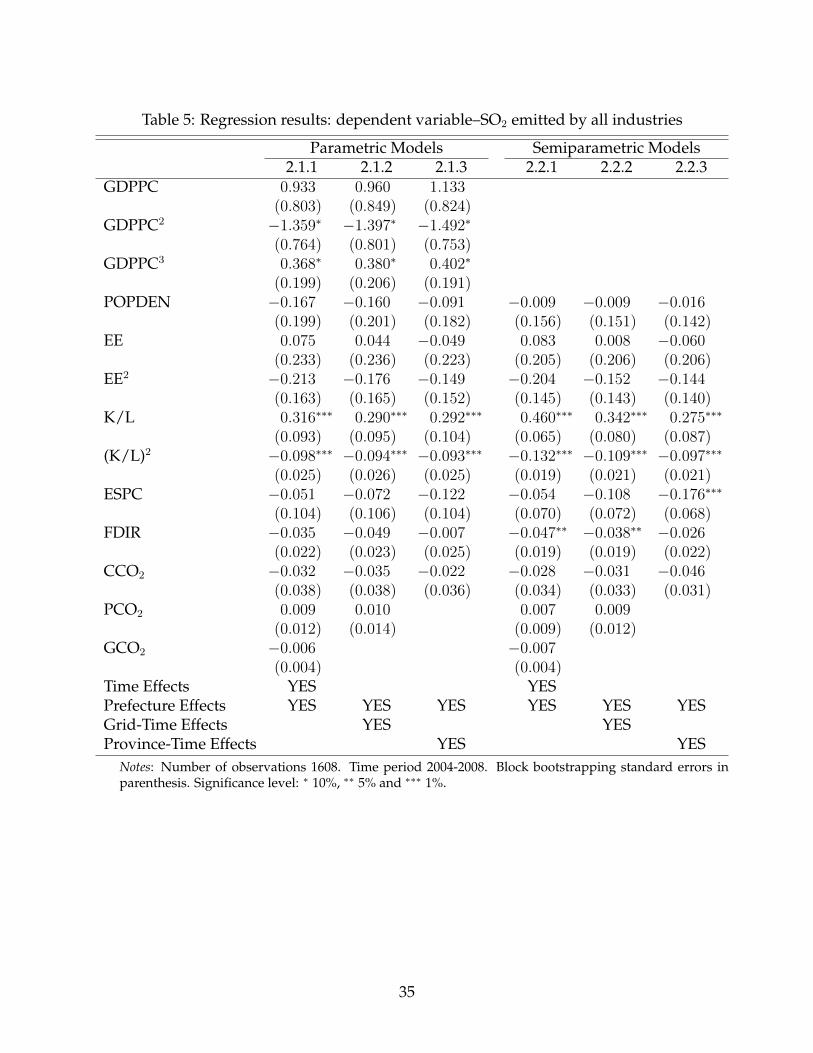
Table 5: Regression results: dependent variable–SO2 emitted by all industries

Parametric Models Semiparametric Models2.1.1 2.1.2 2.1.3 2.2.1 2.2.2 2.2.3

GDPPC 0.933 0.960 1.133(0.803) (0.849) (0.824)

GDPPC2 −1.359∗ −1.397∗ −1.492∗

(0.764) (0.801) (0.753)GDPPC3 0.368∗ 0.380∗ 0.402∗

(0.199) (0.206) (0.191)POPDEN −0.167 −0.160 −0.091 −0.009 −0.009 −0.016

(0.199) (0.201) (0.182) (0.156) (0.151) (0.142)EE 0.075 0.044 −0.049 0.083 0.008 −0.060

(0.233) (0.236) (0.223) (0.205) (0.206) (0.206)EE2 −0.213 −0.176 −0.149 −0.204 −0.152 −0.144

(0.163) (0.165) (0.152) (0.145) (0.143) (0.140)K/L 0.316∗∗∗ 0.290∗∗∗ 0.292∗∗∗ 0.460∗∗∗ 0.342∗∗∗ 0.275∗∗∗

(0.093) (0.095) (0.104) (0.065) (0.080) (0.087)(K/L)2 −0.098∗∗∗ −0.094∗∗∗ −0.093∗∗∗ −0.132∗∗∗ −0.109∗∗∗ −0.097∗∗∗

(0.025) (0.026) (0.025) (0.019) (0.021) (0.021)ESPC −0.051 −0.072 −0.122 −0.054 −0.108 −0.176∗∗∗

(0.104) (0.106) (0.104) (0.070) (0.072) (0.068)FDIR −0.035 −0.049 −0.007 −0.047∗∗ −0.038∗∗ −0.026

(0.022) (0.023) (0.025) (0.019) (0.019) (0.022)CCO2 −0.032 −0.035 −0.022 −0.028 −0.031 −0.046

(0.038) (0.038) (0.036) (0.034) (0.033) (0.031)PCO2 0.009 0.010 0.007 0.009

(0.012) (0.014) (0.009) (0.012)GCO2 −0.006 −0.007

(0.004) (0.004)Time Effects YES YESPrefecture Effects YES YES YES YES YES YESGrid-Time Effects YES YESProvince-Time Effects YES YES

Notes: Number of observations 1608. Time period 2004-2008. Block bootstrapping standard errors inparenthesis. Significance level: ∗ 10%, ∗∗ 5% and ∗∗∗ 1%.

35

Table 6: Regression results: dependent variable–SO2 generated by all industries

Parametric Models Semiparametric Models3.1.1 3.1.2 3.1.3 3.2.1 3.2.2 3.2.3

GDPPC 5.921∗∗∗ 5.758∗∗∗ 6.367∗∗∗

(1.300) (1.362) (1.436)GDPPC2 −3.128∗∗ −3.087∗∗ −3.443∗∗

(1.231) (1.280) (1.311)GDPPC3 0.493 0.496 0.563

(0.320) (0.329) (0.332)POPDEN 0.574∗ 0.522∗ 0.619∗ −0.045 −0.135 −0.016

(0.318) (0.319) (0.315) (0.301) (0.289) (0.283)EE 0.010 −0.057 0.024 0.112 −0.172 0.141

(0.376) (0.380) (0.390) (0.402) (0.400) (0.414)EE2 −0.054 −0.012 −0.051 −0.029 0.072 −0.112

(0.262) (0.264) (0.264) (0.282) (0.276) (0.280)K/L 0.265∗ 0.309∗ 0.091∗ 0.476∗∗∗ 0.282∗ 0.280

(0.155) (0.157) (0.187) (0.129) (0.161) (0.182)(K/L)2 −0.191∗∗∗ −0.203∗∗∗ −0.181∗∗∗ −0.173∗∗∗ −0.145∗∗∗ −0.159∗∗∗

(0.042) (0.042) (0.045) (0.037) (0.041) (0.043)ESPC 0.114 0.085 0.095 0.488∗∗∗ 0.340∗∗ 0.460∗∗∗

(0.166) (0.169) (0.179) (0.135) (0.140) (0.137)FDIR −0.009 −0.009 −0.021 −0.077∗∗ −0.028 −0.031

(0.038) (0.039) (0.046) (0.039) (0.040) (0.049)CCO2 0.187∗∗∗ 0.185∗∗∗ 0.134∗∗∗ 0.202∗∗∗ 0.188∗∗∗ 0.190∗∗∗

(0.061) (0.061) (0.063) (0.066) (0.064) (0.062)PCO2 0.043∗∗ 0.022∗∗ 0.033∗ 0.023

(0.019) (0.023) (0.018) (0.024)GCO2 0.015∗∗ 0.004

(0.006) (0.005)Time Effects YES YESPrefecture Effects YES YES YES YES YES YESGrid-Time Effects YES YESProvince-Time Effects YES YES

Notes: Number of observations 1557. Time period 2004-2008. Block bootstrapping standard errors inparenthesis. Significance level: ∗ 10%, ∗∗ 5% and ∗∗∗ 1%.

36

Table 7: Hypothetical effect of the CDM activity under different baseline sce-narios

Effect of the CDM Activity (wind+coal)Baseline Scenario SO2 Emitted SO2 GeneratedWind/Other Renewable Energy + +Wind+Coal 0 0Natural Gas +/- +/-Coal - -Other Combinations +/- +/-

Notes: The CDM activity is building a wind farm. A companion coal-fired power plantis built for backup supply. Each baseline scenario generates the same electricity output.

37

Figure 1: Shares of CDM projects by types

Hydro

EE own generation

Wind

Coal bed/mine methane

Landfill gas

Biomass energy

Nitrous Oxide

Fossil fuel switch

HFCs

Methane avoidance

EE Industry

EE Supply side

Reforestation

Solar CERs ((kt CO2 e))Number of Projects

0.0

0.1

0.2

0.3

0.4

38

Figure 2: CDM activities in China by the number of projects

Figure 3: CDM activities in China by CERs (103 ton)

39

Figure 4: Nonparametric estimate of the pollution-income relationship m(w)

8 10 12−1

−0.5

0

0.5

Power SO2 E Model 1.2.1

8 10 12−1.5

−1

−0.5

0

Power SO2 E Model 1.2.2

8 10 12−1

−0.5

0

0.5

1

Power SO2 E Model 1.2.3

8 10 120

1

2

3

Ind. SO2 E Model 2.2.1

8 10 12−9

−8.5

−8

−7.5

−7

Ind. SO2 E Model 2.2.2

8 10 12−2

−1

0

1

2

Ind. SO2 E Model 2.2.3

8 10 12−0.5

0

0.5

1

1.5

Ind. SO2 G Model 3.2.1

8 10 12−0.5

0

0.5

1

Ind. SO2 G Model 3.2.2

8 10 12−0.5

0

0.5

1

Ind. SO2 G Model 3.2.3

40