CMPT 889: Lecture 3 Fundamentals of Digital Audio ...tamaras/digitalAudio/digitalAudio.pdf ·...

CMPT 889: Lecture 3Fundamentals of Digital Audio, Discrete-Time Signals

Tamara Smyth, [email protected]

School of Computing Science,

Simon Fraser University

October 6, 2005

1

Sound

• Sound waves are longitudinal waves.

• A disturbance of a source (such as vibrating objects)creates a region of compression that propagatesthrough a medium before reaching our ears.

• More genrally, the source produces alternating regionsof low and high pressure, called rarefactions andcompressions respectively, which propagate through amedium away from the source from some location.

CMPT 889: Computational Modelling for Sound Synthesis: Lecture 3 2

Sound Power and Intensity

• The two physical quantities for a sound wavedescribed so far are the frequency and amplitude ofpressure variations.

• Related to the sound pressure are

1. the sound power emitted by the source

2. the sound intensity measured some distance fromthe source.

• Intensity is given by

I = p2/(ρc)

where ρ is the density of air and c is the speed ofsound.

• The intensity is the power per unit area carried by thewave, measured in watts per square meter (W/m2)

• Intensity therefore, is a measure of the power in asound that actually contacts an area, such as theeardurm.

• The range of human hearing is I0 = 10−12 W/m2

(threshold of audibility) and 1 W/m2 (threshold offeeling).


Linear vs logarithmic scales.

• Human hearing is better measured on a logarithmicscale than a linear scale.

• On a linear scale, a change between two values isperceived on the basis of the difference between thevalues. Thus, for example, a change from 1 to 2would be perceived as the same amount of increase asfrom 4 to 5.

• On a logarithmic scale, a change between two valuesis perceived on the basis of the ratio of the twovalues. That is, a change from 1 to 2 (ratio of 1:2)would be perceived as the same amount of increase asa change from 4 to 8 (also a ratio of 1:2).

Linear

Logarithmic

6543210−1−2−3−4−5−6

1 10 100 1000 10,0000.0001 0.001 0.01 0.1

Figure 1: Moving one unit to the right increment by 1 on the linear scale and multiplies by

a factor of 10 on the logarithmic scale.


Decibels

• The decibel is defined as one tenth of a bel which isnamed after Alexander Graham Bell, the inventor ofthe telephone.

• The decibel is a logarithmic scale, used to comparetwo quantities such as the power gain of an amplifieror the relative power of two sound sources.

• The decibel difference between two power levels ∆Lfor example, is defined in terms of their power ratioW2/W1 and is given in decibels by:

∆L = 10 log W2/W1 dB.

• Since power is proportional to intensity, the ratio oftwo signals with intensities I1 and I2 is similarly givenin decibels by

∆L = 10 log I2/I1 dB.


Sound Power and Intensity Level

• Decibels are sometimes used as absolutemeasurements.

• Though this may seem contadictory (since the decibelis always used to compare two quantities), one of thequantities is really a fixed reference.

• The sound power level of a source, for instance, isexpressed using the threshold of audibilityW0 = 10−12 as a reference and is given in decibels by

LW = 10 log W/W0.

• Similarly, the sound intensity level at some distancefrom the source can therefore be expressed in decibelsby comparing it to a reference—usuallyI0 = 10−12 W/m2:

LI = 10 log I/I0.


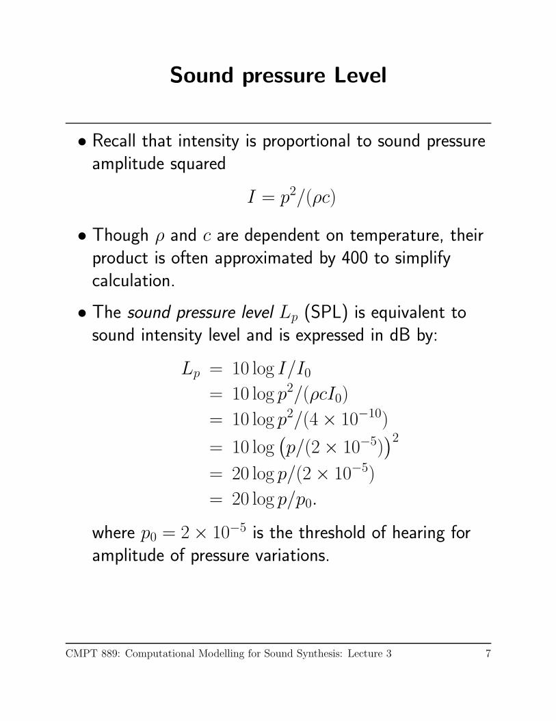
Sound pressure Level

• Recall that intensity is proportional to sound pressureamplitude squared

I = p2/(ρc)

• Though ρ and c are dependent on temperature, theirproduct is often approximated by 400 to simplifycalculation.

• The sound pressure level Lp (SPL) is equivalent tosound intensity level and is expressed in dB by:

Lp = 10 log I/I0

= 10 log p2/(ρcI0)

= 10 log p2/(4 × 10−10)

= 10 log(

p/(2 × 10−5))2

= 20 log p/(2 × 10−5)

= 20 log p/p0.

where p0 = 2 × 10−5 is the threshold of hearing foramplitude of pressure variations.


Continuous vs. Discrete signals

• A signal, of which a sinusoid is only one example, isa set, or sequence of numbers.

• A continuous-time signal is an infinite anduncountable set of numbers, as are the possible valueseach number can have. That is, between a start andend time, there are infinite possible values for time tand instantaneous amplitude, x(t).

• When continuous signals are brought into a computer,they must be digitized or discretized (i.e., madediscrete).

• In a discrete-time signal, the number of elementsin the set, as well as the possible values of eachelement, is finite, countable, and can be representedwith computer bits, and stored on a digital storagemedium.


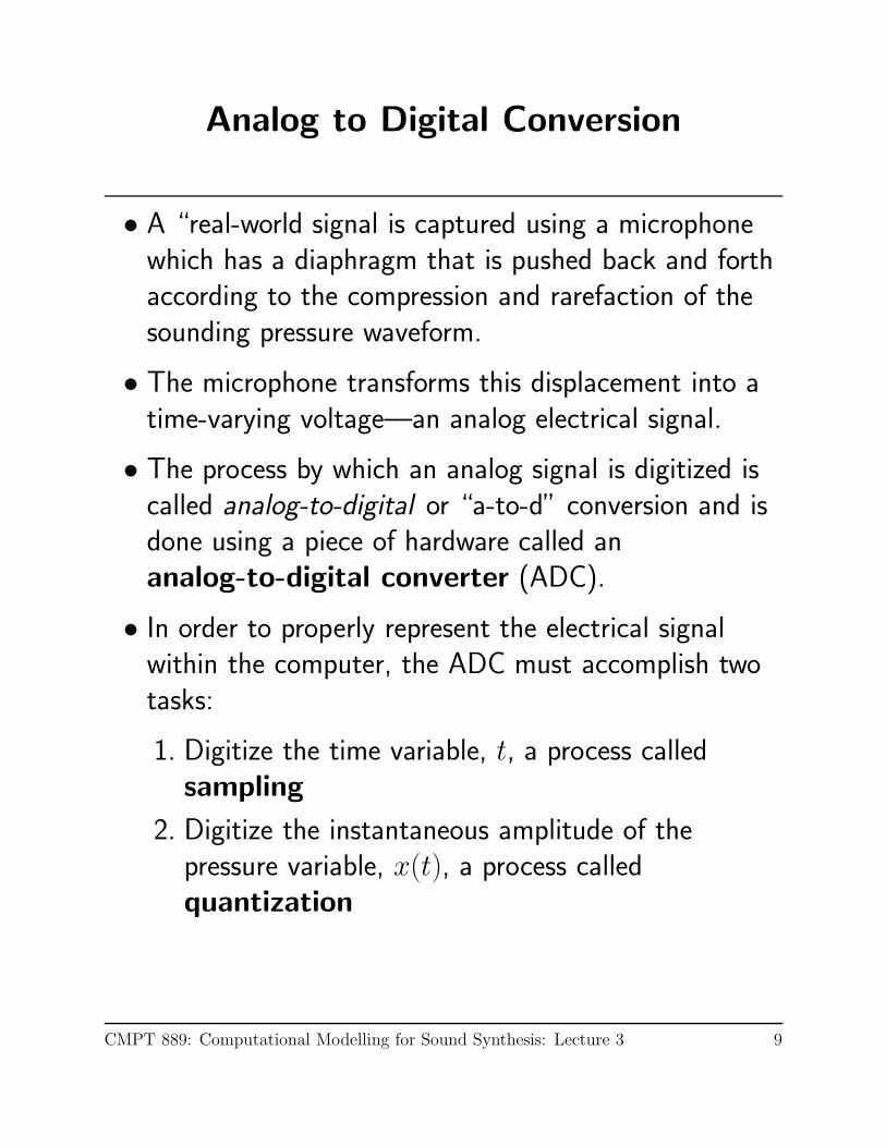
Analog to Digital Conversion

• A “real-world signal is captured using a microphonewhich has a diaphragm that is pushed back and forthaccording to the compression and rarefaction of thesounding pressure waveform.

• The microphone transforms this displacement into atime-varying voltage—an analog electrical signal.

• The process by which an analog signal is digitized iscalled analog-to-digital or “a-to-d” conversion and isdone using a piece of hardware called ananalog-to-digital converter (ADC).

• In order to properly represent the electrical signalwithin the computer, the ADC must accomplish twotasks:

1. Digitize the time variable, t, a process calledsampling

2. Digitize the instantaneous amplitude of thepressure variable, x(t), a process calledquantization


Sampling

• Sampling is the process of taking a sample value,individual values of a sequence, of the continuouswaveform at regularly spaced time intervals.

ADCx(t) x[n] = x(nTs)

Ts = 1/fs

Figure 2: The ideal analog-to-digital converter.

• The time interval (in seconds) between samples iscalled the sampling period, Ts, and is inversely relatedto the sampling rate, fs. That is,

Ts = 1/fs seconds.

• Common sampling rates:

– Professional studio technolgy: fs = 48 kHz

– Compact disk (CD) technology: fs = 44.1 kHz

– Broadcasting applications: fs = 32 kHz


Sampled Sinusoids

• Sampling corresponds to transforming the continuoustime variable t into a set of discrete times that areinteger multiples of the sampling period Ts. That is,sampling involves the substitution

t −→ nTs,

where n is an integer corresponding to the index inthe sequence.

• Recall that a sinusoid is a function of time having theform

x(t) = A sin(ωt + φ).

• In discretizing this equation therefore, we obtain

x(nTs) = A sin(ωnTs + φ),

which is a sequence of numbers that may be indexedby the integer n.

• Note: x(nTs) is often shortened to x(n) (and willlikely be from now on), though in some litteratureyou’ll see square brackets x[n] to differentiate fromthe continuous time signal.


Sampling and Reconstruction

• Once x(t) is sampled to produce x(n), the time scaleinformation is lost and x(n) may represent a numberof possible waveforms.

0 0.2 0.4 0.6 0.8 1 1.2 1.4 1.6 1.8 2−1

−0.5

0

0.5

1Continuous Waveform of a 2 Hz Sinusoid

Time (sec)

Am

plitu

de

0 10 20 30 40 50 60−1

−0.5

0

0.5

1Sampled Signal (showing no time information)

Sample index

Am

plitu

de

0 0.2 0.4 0.6 0.8 1 1.2 1.4 1.6 1.8 2−1

−0.5

0

0.5

1Sampled Signal Reconstructed at Half the Original Sampling Rate

Time (sec)

Am

plitu

de

• If a 2 Hz sinusoid is reconstructed at half thesampling rate at which is was sampled, it will half thefrequency but twice as long.


Sampling and Reconstruction

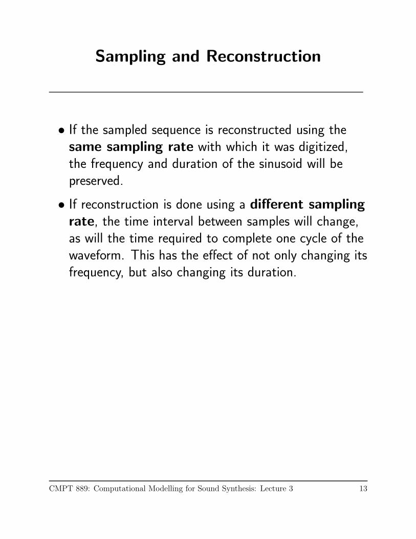
• If the sampled sequence is reconstructed using thesame sampling rate with which it was digitized,the frequency and duration of the sinusoid will bepreserved.

• If reconstruction is done using a different samplingrate, the time interval between samples will change,as will the time required to complete one cycle of thewaveform. This has the effect of not only changing itsfrequency, but also changing its duration.


Nyquist Sampling Theorem

• What are the implications of sampling?

– Is a sampled sequence only an approximation ofthe original?

– Is it possible to perfectly reconstruct a sampledsignal?

– Will anything less than an infinite sampling rateintroduce error?

– How frequently must we sample in order to“faithfully” reproduce an analog waveform?

The Nyquist Sampling Theorem states that:

a bandlimited continuous-time signal can besampled and perfectly reconstructed from itssamples if the waveform is sampled over twice asfast as it’s highest frequency component.


Nyquist Sampling Theorem

• In order for a bandlimited signal (one with afrequency spectrum that lies between 0 and fmax) tobe reconstructed fully, it must be sampled at a rate offs > 2fmax, called the Nyquist frequency.

• Half the sampling rate, i.e. the highest frequencycomponent which can be accurately represented, isreferred to as the Nyquist limit.

• No information is lost if a signal is sampled above theNyquist frequency, and no additional information isgained by sampling faster than this rate.

• Is compact disk quality audio, with a sampling rate of44,100 Hz, then sufficient for our needs?


Aliasing

• To ensure that all frequencies entering into a digitalsystem abide by the Nyquist Theorem, a low-passfilter is used to remove (or attenuate) frequenciesabove the Nyquist limit.

ADC DACCOMPUTERx(nTs)x(t) low−pass

filterlow−pass

filter

Figure 3: Low-pass filters in a digital audio system ensure that signals are bandlimited.

• Though low-pass filters are in place to preventfrequencies higher than half the sampling rate frombeing seen by the ADC, it is possible when processinga digital signal to create a signal containing thesecomponents.

• What happens to the frequency components thatexceed the Nyquist limit?


Aliasing cont.

• If a signal is undersampled, it will be interpreteddifferently than what was intended. It will beinterpreted as its alias.

0 0.1 0.2 0.3 0.4 0.5 0.6 0.7 0.8 0.9 1

−1

−0.5

0

0.5

1

A 1Hz and 3Hz sinusoid

Am

plitu

de

Time (s)

Figure 4: Undersampling a 3 Hz sinusoid causes it’s frequency to be interpreted as 1 Hz.


What is the Alias?

• The relationship between the signal frequency f0 andthe sampling rate fs can be seen by first looking atthe continuous time sinusoid

x(t) = A cos(2πf0t + φ).

• Sampling x(t) yields

x(n) = x(nTs) = A cos(2πf0nTs + φ).

• A second sinusoid with the same amplitude and phasebut with frequency f0 + lfs, where l is an integer, isgiven by

y(t) = A cos(2π(f0 + lfs)t + φ).

• Sampling this waveform yields

y(n) = A cos(2π(f0 + lfs)nTs + φ)

= A cos(2πf0nTs + 2πlfsnTs + φ)

= A cos(2πf0nTs + 2πln + φ)

= A cos(2πf0nTs + φ)

= x(n).


What is an Alias? cont.

• There are an infinite number of sinusoids that willgive the same sequence with respect to the samplingfrequency (as seen in the previous example, since l isan integer (either positive or negative)).

• If we take another sinusoid w(n) where the frequencyis −f0 + lfs (coming from the negative componentof the cosine wave) we will obtain a similar result: ittoo is indistinguishable from x(n).

fs/2 fs 2fs0

Figure 5: A sinusoid and its aliases.

• Any signal above the Nyquist limit will be interpretedas its alias lying within the permissable frequencyrange.


Folding Frequency

• Let fin be the input signal and fout be the signal atthe output (after the lowpass filter). If fin is less thanthe Nyquist limit, fout = fin. Otherwise, they arerelated by

fout = fs − fin.

0 500 1000 1500 2000 25000

500

1000

1500

2000

2500

Folding Frequency fs/2

Folding of Frequencies About fs/2

Out

put F

requ

ency

Input Frequency

Figure 6: Folding of a sinusoid sampled at fs

= 2000 samples per second.

• The folding occurs because of the negative frequencycomponents.


Quantization

• Where sampling is the process of taking a sample atregular time intervals, quantization is the process ofassigning an amplitude value to that sample.

• Computers use bits to store such data and the higherthe number of bits used to represent a value, themore precise the sampled amplitude will be.

• If amplitude values are represented using n bits, therewill be 2n possible values that can be represented.

• For CD quality audio, it is typical to use 16 bits torepresent audio sample values. This means there are65,536 possible values each audio sample can have.

• Quantization involves assigning one of a finite numberof possible values (2n) to the corresponding amplitudeof the original signal. Since the original signal iscontinuous and can have infinite possible values,quantization error will be introduced in theapproximation.


Quantization Error

• There are two related characteristics of a soundsystem that will be effected by how accurately werepresent a sample value:

1. The dynamic range, the ratio of the strongestto the weakest signal)

2. The signal-to-noise ratio (SNR), whichcompares the level of a given signal with the noisein the system.

• The dynamic range is limited

1. at the lower end by the noise in the system

2. at the higher end by the level at which the greatestsignal can be presented without distortion.

• The SNR

– equals the dynamic range when a signal of thegreatest possible amplitude is present.

– is smaller than the dynamic range when a softersound is present.


Quantization Error cont.

• If a system has a dynamic range of 80 dB, the largestpossible signal would be 80 dB above the noise level,yielding a SNR of 80dB. If a signal of 30 dB belowmaximum is present, it would exhibit a SNR of only50 dB.

• The dynamic range therefore, predicts the maximumSNR possible under ideal conditions.



• If amplitude values are quantized by rounding to thenearest integer (called the quantizing level) using alinear converter, the error will be uniformly distributedbetween 0 and 1/2 (it will never be greater than 1/2).

• When the noise is a result of quantization error, wedetermine its audibility using thesignal-to-quantization-noise-ratio (SQNR).

• The SQNR of a linear converter is typicallydetermined by the ratio of the maximum amplitude(2n−1) to maximum quantization noise (1/2).

• Since the ear responds to signal amplitude on alogarithmic rather than a linear scale, it is more usefulto provide the SQNR in decibels (dB) given by

20 log10

(

2n−1

1/2

)

= 20 log10 (2n) .

• A 16-bit linear data converter has a dynamic range(and a SQNR with a maximum amplitude signal) of96dB.

• A sound with an amplitude 40dB below maximumwould have a SQNR of only 56 dB.



• Though 16-bits is usually considered acceptable forrepresenting audio a with good SNQR, its when webegin processing the sound that error compounds.

• Each time we perform an arithmetic operation, somerounding error occurs. Though the operation for oneerror may go unnoticed, the cumulative effect candefinitely cause undesirable artifacts in the sound.

• For this reason, software such as Matlab will actuallyuse 32 bits to represent a value (rather than 16).

• We should be aware of this, because when we write toaudiofiles we have to remember to convert back to 16bits.


CMPT 889: Lecture 3 Fundamentals of Digital Audio ...tamaras/digitalAudio/digitalAudio.pdf ·...

Documents

Transcript of CMPT 889: Lecture 3 Fundamentals of Digital Audio ...tamaras/digitalAudio/digitalAudio.pdf ·...