CMieux 2005: Design and Analysis of

Carnegie Mellon Universitys entry in

the Supply Chain Trading Agent

CompetitionMichael Benisch, Alberto Sardinha,James Andrews and Norman Sadeh

April 2006CMU-ISRI-06-104

Institute for Software Research InternationalSchool of Computer ScienceCarnegie Mellon University

Pittsburgh, PA 15213

The research that lead to the development of the software described in this document has been fundedby the National Science Foundation under ITR Grant 0205435 and under IGERT grant 9972762.

Keywords: Multi-Agent Systems, Supply Chain Management, Trading Agent Design

Abstract

Supply chains are a central element of today’s global economy. Existing management prac-tices consist primarily of static interactions between established partners. Global competi-tion, shorter product life cycles and the emergence of Internet-mediated business solutionscreate an incentive for exploring more dynamic supply chain practices. The Supply ChainTrading Agent Competition (TAC SCM) was designed to explore approaches to dynamic sup-ply chain trading. TAC SCM pits against one another trading agents developed by teamsfrom around the world. Each agent is responsible for running the procurement, planningand bidding operations of a PC assembly company, while competing with others for bothcustomer orders and supplies under varying market conditions. This paper presents CarnegieMellon University’s 2005 TAC SCM entry, the CMieux supply chain trading agent. CMieuximplements a novel approach to coordinating supply chain bidding, procurement and plan-ning, with an emphasis on the ability to rapidly adapt to changing market conditions. Wepresent empirical results based on 200 games involving agents entered by 25 different teamsduring what can be seen as the most competitive phase of the 2005 tournament. Not onlydid CMieux perform among the top five agents, it significantly outperformed these agents inprocurement while matching their bidding performance.

1 Introduction

Existing supply chain management practices consist primarily of static interactions betweenestablished partners [4]. As the Internet helps mediate an increasing number of supplychain transactions, there is a growing interest in investigating the potential for exploring thepotential benefits of more dynamic supply chain practices [1, 12]. The Supply Chain TradingAgent Competition (TAC SCM) was designed to explore approaches to dynamic supply chaintrading. TAC SCM pits against one another trading agents developed by teams from aroundthe world. Each agent is responsible for running the procurement, planning and biddingoperations of a PC assembly company, while competing with others for both customer ordersand supplies under varying market conditions. Specifically, the game features a numberof different types of computers, each requiring different sets of components that can beprocured from multiple suppliers. Agents make money by selling and delivering finishedPCs to customers. Supplier and customer market conditions stochastically change over timeand from one game to another to ensure that agents are tested across a broad range ofrepresentative situations.

This paper presents Carnegie Mellon University’s 2005 TAC SCM entry, the CMieuxsupply chain trading agent. CMieux’s architecture departs markedly from traditional Enter-prise Resource Planning architectures and commercially-available supply chain managementsolutions through its emphasis on tight coordination between supply chain bidding, procure-ment and planning. Through this coordination, our trading agent is capable of adaptingrapdily to changing market conditions and outperform its competitors. In particular, wepresent empirical results based on 200 games involving agents entered by 25 different teamsduring what can be seen as the most competitive phase of the 2005 tournament. Not onlydid CMieux perform among the top five agents, it significantly outperformed these agents inprocurement while matching their bidding performance.

The remainder of this paper is organized as follows. Section 2 summarizes the TAC SCMenvironment, and highlights the features and challenges from a planning and schedulingperspective. Section 3 presents an overview of CMieux and a detailed description of itsunderlying modules. Sections 4 and 5 present empirical results and concluding remarks.

2 TAC Supply Chain Management

This section provides a summary of the TAC Supply Chain Management game. The fulldescription can be found in the official specification document [5].

The TAC SCM game is a simulation of a supply chain where six computer manufactureragents compete with each other for both customer orders and components from suppliers.A server simulates the customers and suppliers, and provides banking, production, andwarehousing services to the individual agents. Every game has 220 simulated days, and each

1

day lasts 15 seconds of real time. The agents receive messages from the server on a dailybasis informing the state of the game, such as the current inventory of components, and mustsend responses to the same server until the end of the day indicating their actions, such asrequests for quotes to the suppliers. At the end of the game, the agent with the highest sumof money is declared the winner.

Normally, each manufacturer agent tackles separately important sub-problems of a supplychain: procurement of components, production and delivery of computers, and computersales. Figure 1 summarizes the high level interactions between the various entities in thegame.

Figure 1: Summary of the TAC SCM Scenario

2.1 Procurement of Components

Each agent is able to produce and store 16 different computer configurations in their ownproduction facility, by using different combinations of components. These computers aremade from four basic components: CPUs, motherboards, memories, and hard drives. Thereare a total of 10 different components: two brands and speeds of CPUs, two brands of moth-erboards, and two sizes of hard disks and memories. The game includes 8 distinct suppliers,and each component has a base price that is used as reference for suppliers making offers.Each PC type also has a base price equal to the sum of the base prices of its components.

Every day, agents can send requests for quotes (RFQs) to suppliers with a given reserveprice, quantity, type and delivery date. A supplier receives all RFQs on a given day, andprocesses them together at the end of the day to find a combination of offers that approxi-mately maximizes its revenue. On the following day, the suppliers send back to each agentan offer for each RFQ with a price, a possibly adjusted quantity, and a due date. Due to

2

capacity restrictions, the supplier may not be able to supply the entire quantity requestedin the RFQ by the due date. Thus, it responds by issuing up to two modified offers, each ofwhich relaxes one of the two constraints:

• Quantity, in which case offers are referred to as partial offers.

• Due date, in which case offers are referred to as earliest offers.

The suppliers have a limited capacity for producing a component, and this limit variesthroughout the game according to a mean reverting random walk. Moreover, suppliers alsolimit their long-term commitments by reserving some capacity for future business. Thepricing of components is based on the ratio of demand to supply, and higher ratios result inhigher prices. Each day the suppliers estimate their free capacity by scheduling productionof components ordered in the past and components requested that day as late as possible.The price offered in response to an RFQ is equal to the requested components base pricediscounted by a function proportionate to the supplier’s free capacity before the RFQ duedate. The manufacturer agents normally face an important trade-off in the procurementprocess: pre-order components for the future where customer demand is difficult to predict,or wait to purchase components and risk being unsuccessful due to high prices or availability.

A reputation rating is also used by the suppliers to discourage agents from driving upprices by sending RFQs with no intention of buying. Each supplier keeps track of its interac-tion with each agent, and calculates the reputation rating based on the ratio of the quantitypurchased to quantity offered. If the reputation falls bellow a minimum value, then theprices and availability of components are affected for that specific agent. Therefore, agentsmust carefully plan the RFQs sent to suppliers.

2.2 Computer Sales

The server simulates customer demand by sending customer requests for quotes (RFQ) to themanufacturer agents. Each customer RFQ contains a product type, a quantity, a due date, areserve price, and a daily late penalty. Moreover, these customer requests are classified intothree market segments: high range, mid range, and low range. Every day, the server sends anumber of RFQs for each segment according to a Poisson distribution, with an average thatis updated on a daily basis by a random walk. The total number of RFQs per day rangesbetween 80 and 320, and demand levels can change rapidly throughout the game. Thus,agents are limited in their ability to plan sales, production and procurement.

The manufacturer agents respond to the customer RFQs by bidding in a first price sealedbid reverse auction: agent’s cannot see competitors bids, and the lowest offer price wins theorder. Agents do receive market reports each day that inform the highest and lowest winningbid prices on the previous day.

3

2.3 Production and Delivery

Each manufacturer agent manages an identical factory, where it can produce any type ofcomputer. The factory is simulated by the game server, and also includes a warehousefor storing components and finished computers. Each computer type requires a specifiednumber of processing cycles, and the factory is also limited to produce 2000 cycles (approx.360 units) per day.

Each day the agent sends a production schedule to the game server, and the simulatedfactory produces computers in the schedule for which the required components are available.A delivery schedule is also sent to the server on a daily basis, and it must specify the productsand quantities of computers to be shipped to each customer order on the following day. Onlycomputers available in inventory can be shipped to customers.

2.4 Related Work

Development teams of TAC SCM agents have proposed several different approaches for tack-ling important sub-problems in dynamic supply chains. Deep Maize [6] uses game theoreticanalysis to factor out the strategic aspects of the environment, and to define an expectedprofitable zone of operation. The agent uses market feedback [8] to dynamically coordinatesales, procurement and production strategies in an attempt to stay in the profitable zone.SouthamptonSCM [7] presents a strategy for using fuzzy reasoning to compute bid prices onRFQs. RedAgent [11] presents an internal market architecture with simple heuristic-basedagents that individually handle different aspects of the supply chain process. TacTex [9]presents machine learning techniques that were extended to form the customer bid priceprobability distributions in CMieux. The TacTex-05 team also offers considerable insightinto the overall strategy behind their first-place agent in [10]. The Botticelli team [3] showshow the problems faced by TAC SCM agents can be modeled as mathematical programmingproblems, and offers heuristic algorithms for bidding on RFQs and scheduling orders.

3 CMieux

A typical supply chain [4] may involve a variety of participants, such as: customers, retail-ers, wholesalers/distributors, manufacturers, and component/raw material suppliers. Theobjective of a supply chain is to maximize the overall value it generates, which is typicallymeasured through profitability.

In a direct sales model [4], such as the one used by Dell Inc., a leading PC distributor,manufacturers fill customer orders directly. Retailers, wholesalers and distributors are by-passed, leaving only three participants - customers, manufacturers and suppliers. This isthe most dynamic supply chain framework presently in use, which is the main reason thatTAC is built around this SCM model. However, TAC SCM goes beyond the limits of present

4

(a) B2C Interaction Overview

(b) B2B Interaction Overview

Figure 2: Primary interactions between modules for B2C and B2B operations in CMieux.

practices by providing manufacturers with the opportunity to simultaneously search daily forthe best supply prices, while concurrently adjusting asking prices based on changing marketconditions.

Competitiveness in dynamic supply chain scenarios, such as those considered in TACSCM, require significantly tighter integration of procurement, bidding and planning func-tionality than implemented in today’s systems [1]. CMieux is dynamic supply chain tradingagent that implements novel adaptive strategies to support this type of integration. In con-trast to many other TAC SCM entries, CMieux continuously re-evaluates both low-levelstrategies, such as its current procurement plan, and high-level strategies, such as its currenttarget market share.

5

3.1 Overview

Figure 2 shows the architecture of our CMieux supply chain trading agent, highlighting keyinteractions between its five main modules. The bidding module is responsible for respondingto customer requests with price quotes. The procurement module sends RFQs to suppliers anddecides which offers to accept. The scheduling module produces a tentative assembly schedulefor several days based on available and incoming resources (i.e. capacity and components).The strategy module makes all high-level strategic decisions, such as what fraction of theassembly schedule should be promised to new customers and what part of the demand tofocus on. The forecasting module is responsible for predicting the prices of components andthe future demand.

Figure 3 gives a general overview of CMieux’s main daily execution path. The agentbegins by collecting any new information from the server, such as the new set of supplieroffers, and customer requests. This information is fed to the forecast module, which updatesits predictions of future demand and pricing trends accordingly. The forecast demand isgiven to the strategy module to determine what part of it our agent should target. Fromthe set of forecast future RFQs the strategy module chooses a subset as the target demand.The procurement module then determines whether or not to accept each newly acquiredsupplier offer. All offers from suppliers are accepted unless they are too late to be useful,or too expensive to remain profitable. The scheduling module builds a tentative tardinessminimizing production schedule for up to twenty days in the future. The schedule includesthe agent’s actual orders, and the future orders composing the target demand. The targetdemand orders are used to determine how many finished PCs the agent has Available toPromise (ATP).

On the Business to Consumer (B2C) side, the strategy module uses the tentative ATPand the forecast selling conditions from the forecasting module to determine what the agentDesires to Promise (DTP). The DTP is used by the bidding module, along with learnedprobabilistic models of competitor pricing. The bidding module chooses prices to maximizethe agent’s expected profit, while offering the amount of products specified by the DTP inexpectation.

The procurement module determines how many components are needed to reach the levelof inventory specified by the strategy module. It compares the desired levels to the projectedlevels, and determines what additional components are needed. Each day the procurementmodule attempts to procure a fraction of the needed components based on the prices andavailability predicted by the forecasting module.

3.2 Forecast Module

The forecast module is an important part of the pro-active planning strategies employedby CMieux. It helps inform a number of key decisions, such as the planning of RFQs sent

6

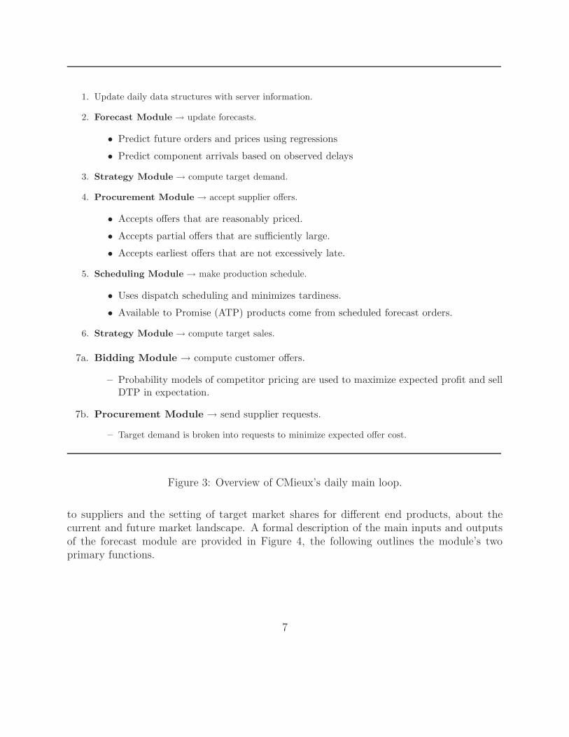
1. Update daily data structures with server information.

2. Forecast Module → update forecasts.

• Predict future orders and prices using regressions

• Predict component arrivals based on observed delays

3. Strategy Module → compute target demand.

4. Procurement Module → accept supplier offers.

• Accepts offers that are reasonably priced.

• Accepts partial offers that are sufficiently large.

• Accepts earliest offers that are not excessively late.

5. Scheduling Module → make production schedule.

• Uses dispatch scheduling and minimizes tardiness.

• Available to Promise (ATP) products come from scheduled forecast orders.

6. Strategy Module → compute target sales.

7a. Bidding Module → compute customer offers.

– Probability models of competitor pricing are used to maximize expected profit and sellDTP in expectation.

7b. Procurement Module → send supplier requests.

– Target demand is broken into requests to minimize expected offer cost.

Figure 3: Overview of CMieux’s daily main loop.

to suppliers and the setting of target market shares for different end products, about thecurrent and future market landscape. A formal description of the main inputs and outputsof the forecast module are provided in Figure 4, the following outlines the module’s twoprimary functions.

7

Forecast Inputs and Constants:

• R, the set of observed customer RFQs.

• OC, the set of customer orders received by the agent.

• OS, the set of supplier orders received by the agent.

• DF, the number of days to forecast into the future.

Forecast Outputs:

• R, a set of RFQs representative of those the agent will see up to DF days in the future.

• fC : j, d → R, a function predicting the selling price of SKU j on day d.

• fS : k, d → R, a function predicting the purchase price of component k on day d.

Figure 4: Forecast module inputs and outputs.

3.2.1 Customer Demand Forecasting

The first responsibility of the forecast module is to predict a set of RFQs representative ofthose our agent expects to see in the future. These RFQs are used by the strategy moduleto determine the agent’s target demand. The forecast module generates a representative setof RFQs by predicting the mean and trend of the customer demand from past observations.Each of the different product grades (high, medium and low) in TAC SCM is governed byits own mean and trend. The actual number of RFQs of each type received each day isdrawn from a Poisson distribution with the mean of that type. The mean for each producttype changes geometrically each day based on the trend (the trend is multiplied by themean and the result is added to the subsequent day’s mean), and the trend is changed bya small amount each day according to a random walk. The forecast module attempts topredict each of the changing mean and trend of the Poisson distribution governing demandseparately, using a linear least squares fit of observations from the past several game days.The predicted trends along with parameters given in the game specification are used togenerate an appropriate set of RFQs.

3.2.2 Price Forecasting

The second responsibility of the forecast module is predicting the selling price of each prod-uct, and the purchasing price of each component up to DF days into the future. This

8

information is useful to several of the other modules in the agent, such as the procurementmodule, that base decisions on current market conditions. The product selling prices arepredicted in the same fashion as the demand trends. A linear least squares (LLSQ) fit iscomputed for the selling prices of each product over the past several game days (addition-ally, we enforce lower and upper bounds on the predictions to ensure they remain relativelyconservative).

The purchasing prices from a particular supplier are predicted using a nearest-neighbor(NN) technique based on historical prices quoted from that supplier. The forecast modulepredicts supplier prices on a particular day in the future by averaging observed quotes withnearby due-dates. Figure 5 shows examples of these two prediction techniques. On anygiven day in TAC SCM the agent is limited to a maximum of 5 requests per supplier andcomponent type. Any of the requests that are unused by the procurement module are usedas probes to aide the NN prediction of the forecast module. The probe dates are chosen toprovide the most information, by picking days that are farthest from existing observations.

30

40

50

60

70

80

90

-10 -5 0 5 10

Cus

tom

er D

eman

d M

ean

Day, d

Forecasting Customer Demand Example

Observed DemandDemand Lower BoundLLSQ Mean Prediction

(a) Customer Demand Forecasting

0.8

1

1.2

1.4

1.6

1.8

2

2.2

2.4

0 5 10 15 20 25

Pur

chas

e P

rice

(fra

ctio

n of

bas

e)

Day, d

Forecasting Supplier Price Prediction Example

Observed PricesNearest Neighbor Predictions

(b) Supplier Price Forecasting

Figure 5: Examples of the techniques used by the forecast module to predict prices.

An additional responsibility of the forecast module is predicting the delays that the agentcan expect on outstanding supplier orders. Suppliers delay the shipment of orders when theircapacity stochastically descends below the level they had previously promised. The forecastmodule predicts the delays on outstanding orders based on the delays observed previouslyfor each supplier and component type. For each product line it determines the delay on themost recent order and propagates it as the expected delay on all other outstanding orders.This relatively simple technique helps the planning aspects of the agent react early to apotential back-log in supplies.

9

3.3 Strategy Module

The strategy module continuously re-evaluates and coordinates strategic decisions, includingsetting market share targets and selling quotas. These targets are continously tweaked toreflect both present and forecast market conditions.

More specifically, the strategy module determines what subset of the forecast customerRFQs the agent should aim to win (the “target demand”) and what fraction of the itsfinished products the agent should plan on selling on any given day (the “desired to promise”products, or DTP). In other words, the strategy module modulates how the output of theforecast module impacts the procurement, scheduling and bidding modules (as illustrated inFigure 2). The primary inputs and outputs of the strategy module are summarized formallyin Figure 6.

Strategy Inputs and Constants:

• O, the set of pending orders.

• R, future customer RFQs from forecast module.

• fC, customer price function from forecast module.

• fS, supplier price function from forecast module.

• SATP, the component of the production schedule from the scheduling module allocated tofuture orders.

Strategy Outputs:

• O, the set of orders representing a target demand, generated from actual orders and forecastfuture RFQs.

• S, quantities of PC that the agent currently desires to promise each day (DTP).

Figure 6: Strategy module inputs and outputs.

3.3.1 Computing Target Demand

On any particular day in the game, the strategy module must first determine the agent’starget demand from the forecast demand. The goal of the strategy module is to target afraction of the forecast demand that will lead to the highest overall profit (this is the agent’sultimate goal). In TAC SCM each agent competes with only five other agents. The agents

10

can significantly impact their own profit margins by flooding or starving a market. Thus,targeting a larger percentage of the forecast will push profit margins down. On the otherhand, agents have a limited factory capacity each day. If products are selling for a profitand factory capacity goes un-utilized, the un-used capacity is lost earning potential. Thiscreates the need for a balance between decreasing target demand to increase profit margins,and still targeting enough demand to maintain high factory utilization.

The strategy module uses a heuristic to address this problem. When products are sellingfor a profit, it always targets exactly enough demand to stay at full utilization. The relativepercentage of each product, or the product mixture, used to fill the target to full capacity isslightly adjusted each day based on the profit margin change of each product type. Whenthe profit margin of a product increases (decreases), its relative percentage in the productmixture increases (decreases) slightly. Figure 7 summarizes this adjustment process for asingle product.

ForecastDemand

forProduct 1

TargetDemand %

+ Profit∆

− Profit∆

Figure 7: The strategy module adjusts the percentage of forecast for each product that enterstarget demand based on change in profit margin.

When a product is no longer being sold for a profit, the strategy module calculatesthe product mixture in the same way. However, the mixture is post-processed so that thecontribution of the unprofitable product is significantly decreased1. This may cause the totaltarget demand to fall below full factory utilization2.

1In practice we found that completely removing unprofitable products from the product mixture providedtoo much of an advantage to competing agents. This motivated our decision to allow the agent to occasionallysell a small percentage of products at a loss.

2During the tail of a game the agent revises this heuristic to ensure it completes the game with as littleinventory as possible

11

3.3.2 Computing Desired to Promise (DTP)

After the target demand is computed by the strategy module, it is used by the schedulingmodule to develop a tentative production schedule for several days into the future (thescheduling window). The scheduling module uses information about incoming and availablecomponents, as well as previously committed orders. Using this information it determineswhen, if at all, each of the target orders will be produced (this process is described inSection 3.4). The part of this schedule assigned to filling target demand orders (as opposedto actual orders) indicates production that is not yet allocated to filling existing customerorders, or the available to promise (ATP) production.

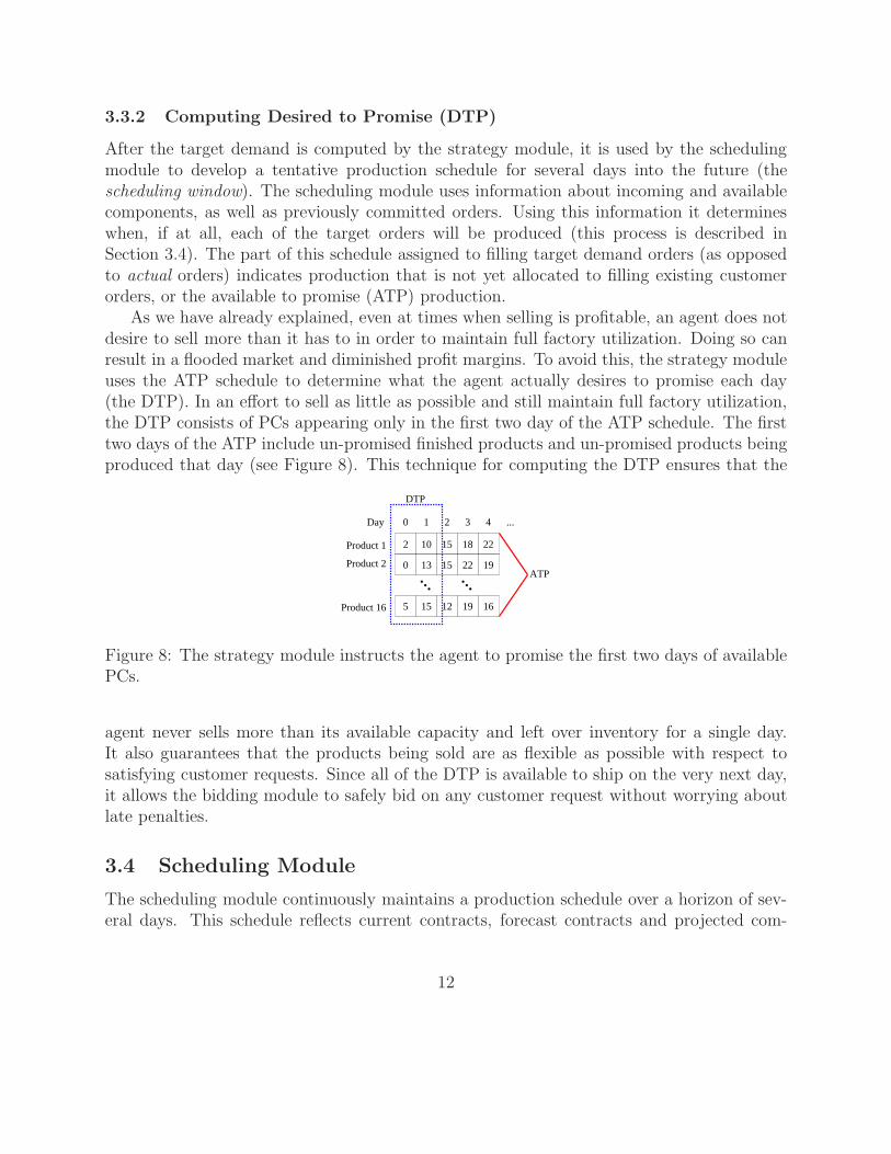
As we have already explained, even at times when selling is profitable, an agent does notdesire to sell more than it has to in order to maintain full factory utilization. Doing so canresult in a flooded market and diminished profit margins. To avoid this, the strategy moduleuses the ATP schedule to determine what the agent actually desires to promise each day(the DTP). In an effort to sell as little as possible and still maintain full factory utilization,the DTP consists of PCs appearing only in the first two day of the ATP schedule. The firsttwo days of the ATP include un-promised finished products and un-promised products beingproduced that day (see Figure 8). This technique for computing the DTP ensures that the

Product 16

10 1815 222

... ...13 150

1912 16

22 19

5 15

Product 1

Product 2

DTP

0 1 3 42 ...Day

ATP

Figure 8: The strategy module instructs the agent to promise the first two days of availablePCs.

agent never sells more than its available capacity and left over inventory for a single day.It also guarantees that the products being sold are as flexible as possible with respect tosatisfying customer requests. Since all of the DTP is available to ship on the very next day,it allows the bidding module to safely bid on any customer request without worrying aboutlate penalties.

3.4 Scheduling Module

The scheduling module continuously maintains a production schedule over a horizon of sev-eral days. This schedule reflects current contracts, forecast contracts and projected com-

12

ponent inventory levels. It helps drive other planning decisions including which customerRFQs to bid on and which RFQs to send to suppliers.

More specifically, the scheduling module makes a tentative production schedule for DS

days into the future. The primary inputs and outputs of the module are summarized formallyin Figure 9. The inputs include a set of orders, O, from the strategy module and the projectedcomponent inventory, I, for the remainder of the game. The orders in O represent the targetdemand of the agent and include both actual and forecast future orders.

Scheduling Inputs and Constants:

• O, a set of orders representing target demand from strategy module, each order i includes thefollowing information:

– di, the due date of the i’th order.

– pi, the daily late penalty associated with the i’th order (the contractual penalty foractual orders and a small constant for forecast orders).

– si, the SKU for the product type associated with the i’th order.

– qi, the quantity of products associated with the i’th order.

– bi ∈ {0, 1}, a flag indicating whether or not the i’th order is an actual order or aforecast order.

• I, the projected component inventory for all remaining days. Idk is the projected inventorylevel of component k on day d.

• DS, number of days in the schedule (scheduling window)

• α, the slack weighting parameter for ATC priorities.

Scheduling Outputs:

• S, a production schedule for DS days, Sd is the set of orders scheduled for production onday d.

Figure 9: Scheduling module inputs and outputs.

3.4.1 Production Scheduling

The scheduling module uses a heuristic to sort orders according to “slack” (time before duedate) and penalty, and a greedy dispatch technique to fill the production schedule. The

13

dispatch technique (presented in pseudo-code in Figure 11) proceeds as follows. It iteratesthrough each day in the scheduling window and computes the priority of each unscheduledorder during each iteration. The priorities are computed according to the Vepsalainen’sapparent tardiness cost (ATC) dispatch rule [13]. The ATC priority favors orders with largepenalties and little time to complete, since these are likely to be orders that require themost immediate attention. The slack weighting parameter, α, dictates the exact trade off inpriority between slack and tardiness. An example of the ATC priorities for different orderswith α = 1 (the value used in our agent) is graphed in Figure 10 as the scheduling dayincreases.

0

0.5

1

1.5

2

2.5

3

2 4 6 8 10 12 14

AT

C O

rder

Prio

rity,

πi

Scheduling Day, d

Example ATC Order Priorities

Due Date = 5, Penalty = 1Due Date = 10, Penalty = 2Due Date = 10, Penalty = 1

Figure 10: Example of ATC priorities for different orders on different scheduling days (α = 1).Notice that ATC prioritizes by penalty once an order’s due date is reached, and by slack fororders with the same penalty.

While building a particular day’s segment of the production schedule, the dispatch sched-uler attempts to add each order to the production schedule according to its priority (orderswith larger priorities are considered first). When an order is considered, the scheduler deter-mines whether or not there are enough available resources (i.e. capacity and components)on the current day of the iteration through the scheduling window. If there are enoughunclaimed resources, the order is scheduled for production and the necessary componentsand production cycles are allocated. If there are not enough resources available on the dayin question, the order is removed from the queue and is considered again the next day. Thescheduler proceeds to the following day when all orders have been considered and eitherscheduled or delayed. This entire process repeats until the scheduling window is exceeded.

3.5 Bidding Module

The bidding module is responsible for responding to a subset of the current customer RFQs.Its goal is to sell the resources specified in the DTP at the highest prices possible. Theinputs and outputs of the bidding module are formally summarized in Figure 12.

14

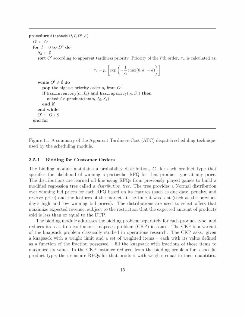
procedure dispatch(O, I, DS, α)

O′ ← Ofor d = 0 to DS do

Sd ← ∅sort O′ according to apparent tardiness priority. Priority of the i’th order, πi, is calculated as:

πi = pi

[

exp

(

−1

αmax(0, di − d)

)]

while O′ 6= ∅ dopop the highest priority order oi from O′

if has inventory(oi, Id) and has capacity(oi, Sd) thenschedule production(oi, Id, Sd)

end ifend whileO′ ← O \ S

end for

Figure 11: A summary of the Apparent Tardiness Cost (ATC) dispatch scheduling techniqueused by the scheduling module.

3.5.1 Bidding for Customer Orders

The bidding module maintains a probability distribution, G, for each product type thatspecifies the likelihood of winning a particular RFQ for that product type at any price.The distributions are learned off line using RFQs from previously played games to build amodified regression tree called a distribution tree. The tree provides a Normal distributionover winning bid prices for each RFQ based on its features (such as due date, penalty, andreserve price) and the features of the market at the time it was sent (such as the previousday’s high and low winning bid prices). The distributions are used to select offers thatmaximize expected revenue, subject to the restriction that the expected amount of productssold is less than or equal to the DTP.

The bidding module addresses the bidding problem separately for each product type, andreduces its task to a continuous knapsack problem (CKP) instance. The CKP is a variantof the knapsack problem classically studied in operations research. The CKP asks: givena knapsack with a weight limit and a set of weighted items – each with its value definedas a function of the fraction possessed – fill the knapsack with fractions of those items tomaximize its value. In the CKP instance reduced from the bidding problem for a specificproduct type, the items are RFQs for that product with weights equal to their quantities.

15

Bidding Inputs and Constants:

• R, the set of current RFQs.

• G : r, p → (0, 1), a cumulative density function that takes an RFQ, r, and a unit price, p,and provides the probability that the winning price for r will be greater than p.

• G−1 : r, (0, 1) → p, the inverse of G, takes an RFQ and a probability and returns thecorresponding price.

• S, the DTP from strategy module.

Bidding Outputs:

• F C, a set of offers for customers. Each offer corresponds to an RFQ in R, and includes aunit price.

Figure 12: Bidding module inputs and outputs (G and G−1 are maintained internally).

The weight limit in the CKP is the quantity of the product appearing in the DTP. The valueof a fraction, x, of an RFQ, r, is the expected unit revenue that yields a winning probabilityof x. The expected unit revenue is defined as the probability with which the customer isexpected to accept the offer (as specified by the bidding module’s probability distribution)times the offer price, G−1(r, x)× x.

CMieux uses a binary search algorithm to solve the CKP instance for each productthat is guaranteed to provide a solution within ǫ of optimal expected revenue. The searchalgorithm operates on the derivatives of the expected unit revenue functions. It finds thelargest derivative value corresponding to a solution that does not violate the weight limit ofthe knapsack. Since the distributions are Normal the expected unit revenue functions arestrictly concave, and the solution corresponding to the largest feasible derivative value isoptimal. For full descriptions of the reduction to a CKP, the ǫ-optimal algorithm, and theprobability distributions used in CMieux the reader is directed to [2]3.

3.6 Procurement Module

The procurement module handles all aspects of requesting and purchasing components. Itis designed to rapidly adapt to changing market conditions. Each day, it considers sendingrequests with widely varying quantities and lead times in an effort to exploit gaps in currentsupplier contracts. By finding such gaps, or slow days for the suppliers, the agent ensures

3A sister paper based on this technical report has also been submitted to ICEC’06.

16

that its procurement prices tend to fall below its competitors. The flexibility gained byconsidering so many different procurement strategies in this way sets CMieux apart frommost existing supply chain practices, as well as those of other agents designed for TAC SCM.

Each day, the procurement module performs two tasks: i.) it attempts to identify aparticularly promising subset of current supplier offers, and ii.) it constructs a combinationof RFQs to be sent to suppliers that balances the agent’s component needs with identifiedgaps in current supplier contracts.

The procurement module takes as input the set of recent supplier offers, the projectedinventory, the target demand and the forecast pricing functions (see Figure 13).

Procurement Inputs and Constants:

• F S, the set of offers from suppliers.

• I, the projected component inventory for all remaining days. Ikd is the projected inventorylevel of component k on day d.

• O, target demand from strategy module.

• fC, customer price function from forecast module.

• fS, supplier price function from forecast module.

• 〈D−, D+, DG〉, the earliest, and latest days to consider requesting for, and the granularityto discretize search.

• KS, the number of requests allowed per supplier.

Procurement Outputs:

• F , the set of supplier offers to accept.

• Z, the procurement requests for each supplier. Zlk = {z1, . . . , zKS} is the set of requestsfor supplier l and component k. Each request includes the following information:

– qi, the quantity of the request.

– di, the due date of the request.

– ri, the reserve price of the request.

Figure 13: Procurement module inputs and outputs.

17

3.6.1 Accepting Supplier Offers

The module accepts supplier offers using a rule-based decision process. The agent begins byselecting offers that are satisfactory based on price, quantity and due date using historicaldata. In an effort to keep the agent’s reputation as high as possible4, the agent first acceptsoffers that satisfy the quantity and due date requirements of the corresponding RFQ (“fulloffers”). Next, if still needed, satisfactory offers with relatively large quantities (“partialoffers”), or early due dates (“earliest complete offers”) are also accepted.

3.6.2 Sending Supplier Requests

Since offer prices, due dates and quantities are dictated by the specific requests they areoffers for, the primary responsibility of the procurement module is requisitioning. The req-uisitioning procedure used in CMieux attempts to request some of the components it needs(that it has not already purchased) to maintain its target production levels, each day. Itsmain goal is to ensure that the prices offered in response to the requests are as low as possi-ble. The requisitioning procedure chooses between many different lead times and quantities,based on the forecast supplier market landscape.

In order to determine what requests to send to suppliers, the procurement module com-putes, I, the difference between the inventory required to maintain production levels specifiedby the target demand, and the projected inventory for the remainder of the game (i.e. thecomponents that it needs but has not yet purchased). However, our agent does not need toprocure this entire difference each day. The components are not needed immediately, thus itcan divide the purchasing of components in I across several days. To that end, the quantitiesspecified in I beyond DS days in the future (the scheduling window) are linearly depleted.This enables the agent to aggressively procure components within its scheduling window, sothat late penalties are not incurred on existing contracts. In addition, it allows the agent tobuy some of the components it needs well in advance, when they are likely to be cheapest.

The process of computing what specific requests to send to suppliers is then decomposedby component type. For each component type, the procurement module generates severalsets of KS(the limit on RFQs sent each day) lead times and searches for the best set.

More specifically, the module uses brute force to enumerate all ways to choose a tupleof KS + 1 dates between D− and D+, discretized by DG. The first KS dates in the tuplespecify the RFQ lead times. Each of the RFQs requests the components needed by the agentbetween its lead time, and the next date in the tuple (this is why there must be one morethan KS dates in the tuple).

For example, if D− = 5, D+ = 20, DG = 5, and KS = 2, then the procurement modulewould consider the following tuples of dates 〈5, 10, 15〉, 〈5, 10, 20〉, 〈5, 15, 20〉 and 〈10, 15, 20〉.Each RFQ is used to procure the parts specified in I between its due date and the subsequent

4Maintaining a perfect reputation was identified as an important strategic goal for the 2005 competition.

18

procedure request(I, O, f C, f S, 〈D−, D+, DG〉, KS)

let I be a fraction of the difference between in-ventory maintaining production levels of O, andinventory available in I.for each component, k do

d∗ ← {}

u∗ ← 0KS−1

for each set of KS + 1 dates, {d1, . . . , dKS+1},between D− and D+, discretized by DG do

u← approx utility({d1, . . . , dKS+1}, I, k, fC, f S)if sum(u) > sum(u∗) then

d∗ ← {d1, . . . , dKS+1}u∗ ← u

end ifend forfor i = 1 to KS do

let l be the supplier of k with the lowest priceon day di

qi ←∑di+1

d=diIkd

zi ← 〈di, qi, u∗i /qi〉

Zlk ← Zlk ∪ {zi}end for

end forreturn Z

procedure approx utility({d1, . . . , dKS+1}, I, k, fC, f S)

u← 0KS

let J be the products containing component kfor j ∈ J do

let βj and βk be base prices of product j andcomponent k from the game specificationfor i = 2 to KS + 1 do

d← di−1

while d < di do

u←(

βk

βjf C(j, d)

)

− f S(k, d)

ui−1 ← ui−1 + Ikdu|J|

d← d + 1end while

end forend forreturn u

Figure 14: Pseudo-code for the requisitioning procedure used by the procurement module.

due date in the tuple. Consider the tuple 〈5, 10, 15〉, which involves two RFQs. The first hasa lead time of 5 and a quantity equal to the sum of the parts specified in I between 5 and10 days in the future. The second RFQ has a lead time of 10 and a quantity equal to thesum of the parts specified in I between 10 and 15 days in the future.

The utility of the RFQs generated by each tuple is computed by approximating the sumof the utility of the components they request and subtracting their forecast prices. In orderto approximate the utility of a component, k, we compute the ratio between its base price,βk, and the base price of each product, j, it is included in, βj. The base price ratio, βk

βj,

provides an approximation of the fraction of product j’s revenue attributable to componentk. Thus, the utility of a component is approximated as the average selling price, weightedby the base price ratio, of each of the products it is included in. The cost of each RFQ isgiven by the supplier pricing forecast function, f S.

19

The RFQs with the greatest utility for each component are sent to the appropriatesuppliers. The reserve price of each RFQ is set to be the average utility of the componentsit includes. Figure 14 provides pseudo-code outlining this requisitioning process.

In addition, we augmented this flexible and dynamic requisitioning procedure with thefollowing improvements.

Increased bottleneck component utility: The utility of a component can be furtherrefined by taking into account situations where the agent has all but one of the componentsrequired to assemble a particular type of PC (making it a bottleneck component). This sit-uation can become more severe toward the end of the game as the agent faces the prospectof being stuck with mis-matched components. For example, our agent can have hundreds ofmotherboards, memory, and CPUs to make a specific product, and be missing only the harddrives. To address this issue, the procurement module artificially inflates the base price ratioof bottleneck components (such as the hard drives in the example), and decreases the baseprice ratio of all other components5. The inflation factor is increased as the agent nears theend of the game.

Dynamically refined search granularity: An additional observation was that, for shortlead times, supplier pricing was often drastically different even between lead times as littleas 1 day apart. In practice, our agent used a search granularity of about DG = 5 days, whichcaused it to frequently miss promising early lead times. To address this issue, after findingthe most promising lead time tuple at a particular granularity our agent generated new setsof tuples using finer and finer granularity around previously identified promising tuples. Thishelped the agent more effectively cover the space without drastically effecting its runtime.

Parallelization across components: The requisitioning technique described above de-composes its search through lead time tuples by component type. In order to give our agentthe ability to perform a finer search we parallelized the requisitioning process across mul-tiple CPUs, each of which was responsible for considering a subset of components. Due tothe natural decomposition of our problem formulation, the parallel processes had no needto interact (other than to aggregate their final solutions) making this a relatively simplerefinement to implement.

4 Empirical Evaluation

To validate the adaptive and dynamic techniques utilized in our agent we present two sets ofempirical results. The first, and more important set of results are taken from the 2005 TAC

5This can be thought of as a coarse approximation of a component’s marginal utility

20

SCM seeding rounds6, and summarize CMieux’s bidding and procurement performance over200 games involving agents entered by 25 different teams. A second set of results is alsopresented that examines the accuracy of our forecast module when it comes to predictingsupplier prices and customer demand. This includes looking at how well a top performingagent such as CMieux is able to predict supplier prices using the limited number of RFQsallowed by the game specifications as well as how accuracy is affected by the forecast horizonin different game phases.

4.1 Procurement and Bidding Performance

Evaluating the performance of a supply chain trading agent is challenging even in the contextof TAC SCM. The competition effectively consists of two different tournaments:

1. a seeding round tournament featuring a large number of agents competing over a periodof 2 weeks in about 400 games

2. a set of final rounds, where small sets of agents are pitted against one another in arelatively limited number of games (ranging from 8 to 16 per round).

Not only do they feature a small number of games but, because they repeatedly pit the sameagents against one another, final rounds also potentially reward destructive strategies thatmay not be representative of real world competition (e.g. an agent disrupting competitorsat the expense of its own bottom line). In 2005, CMieux finished 4th in the seeding roundsand reached the tournament’s semi-finals. While encouraging, these results only provide apartial picture of CMieux’s performance. In this section, we provide a more in-depth analysisof our agent during what can be viewed as the most competitive phase of the competition,namely the 200 games played by the 25 agents participating in the second week of the seedingrounds. All agents at that stage have already been fine tuned over the course of about 600games (two weeks of qualifying rounds, and one week of seeding).

Specifically, our results provide a statistical comparison between the performance of theagents with the top 5 mean overall scores during the second week of the seeding rounds,namely CMieux (abbreviated CM), FreeAgent (FA), GoBlueOval (GBO), MinnieTAC (MT)and TacTex-05 (TT).

Performance was measured so as to identify those agents that were able to extract thehighest sale price and lowest purchasing price in each game they played. Specifically, foreach of the top 5 agents in each game it played in we computed how far it was from payingthe least for its components and obtaining the most for its end products among the agentsplaying in that particular game. This was measured as the relative difference from the bestaverage procurement price7 and the best average selling price. For each of the top 5 agents

6Competition data is available at sics.se/tac/scmserver7All prices are considered as fractions of the corresponding product or component’s base price.

21

we report the mean (with 95% confidence intervals) of these values across all of the gamesthey each played in (see Figure 15).

0

0.01

0.02

0.03

0.04

0.05

0.06

0.07

0.08

TTMTGBOFACM

Diff

eren

ce (

Fra

c. o

f Bas

e P

rice) Bidding

(a) Bidding Analysis

0

0.01

0.02

0.03

0.04

0.05

0.06

0.07

0.08

TTMTGBOFACM

Diff

eren

ce (

Fra

c. o

f Bas

e P

rice) Procurement

(b) Procurement Analysis

Figure 15: The mean (with 95% confidence intervals) difference between each of the top 5agents’ average game unit price and the best unit price in the game, during the second weekof the 2005 TAC SCM seeding rounds.

The bidding results for all 5 agents are relatively similar. As can be seen, each of thetop 5 agents is on average within about 3% of the base price from being the best in itsgames. However, while MinnieTAC (MT) was the closest to the best agent in its games,with an average difference of about 2% of the base price, there is no statistically significantdifference between any of the top 5 agents (as evidenced by their overlapping confidenceintervals). On the other hand, the procurement results show that our agent, CMieux (CM),is significantly closer to being the best than all 4 of the other top 5 agents. These results seemto validate CMieux’s approach to tightly coordinating its bidding, planning and procurementoperations. They also suggest that the agent’s approach to optimizing the RFQs it sends tosuppliers (requisition process) was significantly more effective than the procurement strategiesimplemented by its competitors.

4.2 Forecast Accuracy

In this section, we report additional results investigating how well a top performing agentsuch as CMieux can predict supplier prices and customer demand, given the high degreeof stochasticity associated with these markets. This includes looking at how well the agentis able to predict supplier prices, given the limited number of RFQs allowed by the gamespecifications as well as how accuracy is affected by the forecast horizon in different gamephases.

22

Results reported below were obtained by pitting CMieux against 5 publicly availableagents8, namely TacTex-05, Phantagent, Mertacor, CrocodileSCM, GoBlueOval. All 5 ofthese agents were among those qualifying for the final rounds of the 2005 competition.

0

0.02

0.04

0.06

0.08

0.1

5 10 15 20 25 30 35 40

Err

or (

Fra

c. o

f Bas

e P

rice)

Lead Time (d)

Error in Forecast

Early GameMid GameEnd Game

(a) Error in component price forecast as a functionof lead time in different game segments.

0

0.02

0.04

0.06

0.08

0.1

5 10 15 20 25 30 35 40

Err

or (

Fra

c. o

f Bas

e P

rice)

Lead Time (d)

Error in Forecast

Early GameBaseline

(b) Error of early segment component price predic-tion with baseline that used unlimited probes.

0

50

100

150

200

0 100 200 300 400 500

Cus

tom

er D

eman

d M

ean

Time Step

Forecast and Actual Demand Mean

Actual DemandLR Forecast

(c) Example: forecast and actual customer demandmean.

Figure 16: Empirical evaluation of the forecast module.

Figure 16(a) plots CMieux’s error in predicting supplier prices during the early, mid, andlate segments of the games as a function of lead time. For comparison purposes, the resultsin Figure 16(b) show the error of the early segment predictions of both CMieux’s forecastingtechnique and a baseline variant that relaxes the game’s restriction on the number of probesthat can be sent by an agent - results for the mid and end game phases are similar. Theplots provide the mean error (with 95% confidence intervals) as a fraction of component

8Agents are available at sics.se/tac/showagents.php

23

base price of all component price forecasts made during those segments. The predictionerror is measured for each possible lead time between 5 and 40 days at 5 day intervals. Theresults show that the early segment of the game is the most difficult segment for CMieux’sforecast module to accurately predict supplier pricing, for all lead times. Even the baselinevariant with unlimited number of probes is unable to achieve high accuracy during thissegment. This is not surprising considering that agents are not likely to have settled into anequilibrium yet and are reacting to start up effects (effects introduced by the fact that allagents begin the game with no components). Additionally, we can see that both our techniqueand the baseline variant have more error when predicting prices on orders with shorter leadtimes during all game segments. The difficulty of predicting prices with short lead times isexaggerated during the early segment due to the previously mentioned instability. Despitethe instability we see that the greatest error in the supplier price forecasting is only about10% of the base price, resulting from the prediction of short lead time prices during the earlysegment of the game. Forecasting of orders with longer lead times, and short lead times laterin the game, is generally accurate within 95% of the base price.

Figure 16(c) shows an example of a changing customer demand mean, and the predictionsof the forecast module based on observations of draws from a Poisson distribution with thatmean. The results on this particular example show that the forecast module is relativelyeffective at predicting the mean and following its trend. To gain a better understanding ofthe effectiveness of our forecast module for predicting customer demand, we compared it to anaive technique that assumed the current mean was the most recently observed sample fromthe Poisson distribution. A more detailed analysis of our technique and the naive techniqueacross multiple games revealed that on average our forecast module was within 7% (plusor minus 1% with 95% confidence) and the naive technique was within 12% (plus or minus1% with 95% confidence) of properly predicting the mean of each product type’s demanddistribution. While this result does not show a largely significant difference between ourforecast module and the naive technique, our forecast module was much better at predictingthe trends of the means. Our technique was within 2% (plus or minus less than 1% with 95%confidence) of predicting the trends on average, whereas the naive technique had an averageof about 18% (plus or minus 2% with 95% confidence) error when predicting the trends.

5 Conclusions

This paper presented a high level view of the interactions between the different modulescomposing CMieux, Carnegie Mellon University’s 2005 TAC SCM entry, as well as detaileddescriptions of its decision making processes. CMieux’s architecture departs markedly fromtraditional Enterprise Resource Planning architectures and commercially-available supplychain management solutions through its emphasis on tight coordination between supplychain bidding, procurement and planning.

24

CMieux finished 4th in the 2005 seeding rounds of the TAC SCM tournament and reachedthe competition’s semifinals. In this paper, we presented a more in-depth analysis of theagent’s performance based on 200 games involving agents entered by 25 different teams dur-ing what can be seen as the most competitive phase of the 2005 tournament. The resultsshow that our agent performed on par with the best in its bidding while significantly out-performing these agents in terms of procurement. These results seem to validate CMieux’sapproach to tightly coordinating its bidding, planning and procurement operations. Theyalso suggest that the agent’s approach to optimizing the RFQs it sends to suppliers (requi-sition process) was significantly more effective than the procurement strategies implementedby its competitors.

References

[1] R. Arunachalam and N. Sadeh. The supply chain trading agent competition. Electronic

Commerce Research Applications, 4(1), 2005.

[2] M. Benisch, J. Andrews, and N. Sadeh. Pricing for customers with probabilistic valu-ations as a continuous knapsack problem. Technical Report CMU-ISRI-05-137, Schoolof Computer Science, Carnegie Mellon University, December 2005.

[3] M. Benisch, A. Greenwald, I. Grypari, R. Lederman, V. Naroditsky, and M. Tschantz.Botticelli: A supply chain management agent. In Third International Joint Conference

on Autonomous Agents and Multi-Agent Systems, 2004.

[4] S. Chopra and P. Meindl. Supply Chain Management. Pearson Prentice Hall, NewJersey, 2004.

[5] J. Collins, R. Arunachalam, N. Sadeh, J. Eriksson, N. Finne, and S. Janson. The supplychain management game for 2005 trading agent competition, 2005.

[6] J. Estelle, Y. Vorobeychik, M. P. W. S. Singh, C. Kiekintveld, and V. Soni. Strategicinteractions in a supply chain game, 2003.

[7] M. He, A. Rogers, X. Luo, and N. R. Jennings. Designing a successful trading agent forsupply chain management. In Proceedings of AAMAS’06, 2006.

[8] C. Kiekintveld, M. P. Wellman, S. Singh, J. Estelle, Y. Vorobeychik, V. Soni, andM. Rudary. Distributed feedback control for decision making on supply chains. InFourteenth International Conference on Automated Planning and Scheduling, 2004.

[9] D. Pardoe and P. Stone. Bidding for customer orders in tac scm. In AAMAS-04

Workshop on Agent-Mediated Electronic Commerce, 2004.

25

[10] D. Pardoe and P. Stone. Predictive planning for supply chain management. In Proceed-

ings of Automated Planning and Scheduling’06, 2006.

[11] D. P. Philipp W. Keller, Felix-Olivier Duguay. Redagent-2003: An autonomous, market-based supply-chain management agent. In Third International Joint Conference on

Autonomous Agents and Multi-Agent Systems, 2004.

[12] N. Sadeh, D. Hildum, D. Kjenstad, and A. Tseng. Mascot: an agent-based architecturefor coordinated mixed-initiative supply chain planning and scheduling. In Proceedings of

Workshop on Agent-Based Decision Support in Managing the Internet-Enabled Supply-

Chain at Agents’99, 1999.

[13] A. Vepsalainen and T. Morton. Priority rules for job shops with weighted tardinesscosts. Management Science, 33(8):1035–1047, 1987.

26