
CLUTTER DETECTION IN PULSE-DOPPLER RADAR … · CLUTTER DETECTION IN PULSE-DOPPLER RADAR SYSTEMS...
80
CLUTTER DETECTION IN PULSE-DOPPLER RADAR SYSTEMS a thesis submitted to the department of electrical and electronics engineering and the institute of engineering and sciences of bilkent university in partial fulfillment of the requirements for the degree of master of science By Ahmet G¨ ung¨ or August 2010
Transcript of CLUTTER DETECTION IN PULSE-DOPPLER RADAR … · CLUTTER DETECTION IN PULSE-DOPPLER RADAR SYSTEMS...
CLUTTER DETECTION IN PULSE-DOPPLER
RADAR SYSTEMS
a thesis
submitted to the department of electrical and
electronics engineering
and the institute of engineering and sciences
of bilkent university
in partial fulfillment of the requirements
for the degree of
master of science
By
Ahmet Gungor
August 2010

I certify that I have read this thesis and that in my opinion it is fully adequate,
in scope and in quality, as a thesis for the degree of Master of Science.
Assist. Prof. Dr. Sinan Gezici (Supervisor)
I certify that I have read this thesis and that in my opinion it is fully adequate,
in scope and in quality, as a thesis for the degree of Master of Science.
Prof. Dr. Orhan Arıkan
I certify that I have read this thesis and that in my opinion it is fully adequate,
in scope and in quality, as a thesis for the degree of Master of Science.
Assist. Prof. Dr. Ibrahim Korpeoglu
Approved for the Institute of Engineering and Sciences:
Prof. Dr. Levent OnuralDirector of Institute of Engineering and Sciences
ii
ABSTRACT
CLUTTER DETECTION IN PULSE-DOPPLER
RADAR SYSTEMS
Ahmet Gungor
M.S. in Electrical and Electronics Engineering
Supervisor: Assist. Prof. Dr. Sinan Gezici
August 2010
Among various types of radar systems, the pulse-Doppler radar is the most widely
used one, especially in military applications. Pulse Doppler radars have a pri-
mary objective to detect and estimate the range and the radial velocity of the
targets. In order to have a basis for the detection, first reflected echo signals are
matched filtered and then the time-alligned pulse returns are transformed to the
Fourier domain to obtain the range-Doppler matrix. The resulting range-Doppler
matrix is input to target detection algorithms. For this purpose, constant false
alarm rate (CFAR) algorithms are run on the range-Doppler matrix. It is useful
to run different CFAR algorithms inside the clutter region and outside the clutter
region because the statistics are different inside and outside of the clutter. In or-
der to achieve this discrimination, the position of the clutter has to be detected in
the range-Doppler matrix. Moreover, the clutter may not always appear around
zero Doppler frequency when realistic terrain models and moving platforms are
considered. Two algorithms for clutter detection using range-Doppler matrix ele-
ments are investigated and their performance analysis is presented in this thesis.
The first algorithm has higher error rates but lower computational complexity,
iii
whereas, the second one has lower error rates but higher computational com-
plexity. Both algorithms detect clutter position by filtering the range-Doppler
matrix elements via non-linear filters. In addition to the probabilistic error rate
analysis, simulation results on some realistic cases are presented. It is concluded
that the first algorithm is a good choice for low clutter-to-noise ratio values when
a low-complexity algorithm is required. On the other hand, the second algorithm
has better performance in all clutter-to-noise ratio values but it requires more
computational power.
Keywords: Pulse-Doppler Radar, Realistic Terrain Generation, Matched Filter-
ing, Pulse-Doppler Processing, Clutter Detection, Kernel Density Estimation,
Kullback-Leibler Divergence.
iv
OZET
DARBE-DOPPLER RADAR SISTEMLERINDE PARAZIT
YANKI TESPITI
Ahmet Gungor
Elektrik ve Elektronik Muhendisligi Bolumu Yuksek Lisans
Tez Yoneticisi: Yrd. Doc. Dr. Sinan Gezici
Agustos 2010
Cesitli radar sistemleri arasında darbe Doppler radar sistemleri, ozellikle
askeri uygulamalarda en cok kullanılanıdır. Darbe Doppler radar sistemlerinin
birincil gorevi hedefleri tespit edip, hedeflerin menzil ve radyal hızlarını ke-
stirmektir. Tespit yapabilmek icin, yansıyan sinyaller uyumlu suzgecten gecirilip,
darbe Doppler islemine tabi tutulur. Sonucta elde edilen mesafe-Doppler matrisi
bazı tespit algoritmalarına girdi olarak kullanılır. Hedefleri tespit edebilmek icin,
Sabit Yanlıs Alarm Oranlı (SYAO) algoritmalar mesafe-Doppler matrisi uzerinde
kosturulur. Parazit yankı bolgesinde ve bu bolgenin dısında farklı SYAO algo-
ritmaları kosturmak yararlıdır. Cunku hucre istatistigi parazit yankının icinde
ve dısında farklıdır. Bu ayrımı elde edebilmek icin oncelikle mesafe-Doppler
matrisinde parazit yankının yeri tespit edilmelidir. Gercekci arazi modelleri ve
hareketli platformlar goz onune alındıgında, parazit yankı sıfır Doppler frekansı
etrafında bulunmayabilir. Bu tez calısmasında, mesafe-Doppler matrisi eleman-
larını kullanarak, parazit yankı tespit edilmesine yonelik iki algoritma ve per-
formans analizleri sunulmaktadır. Algoritmalardan birincisi daha yuksek hata
oranına ancak daha dusuk islem karmasıklıgına, ikincisi ise daha dusuk hata
v
oranına ancak daha yuksek islem karmasıklıgına sahiptir. Algoritmalar mesafe-
Doppler matrisi elemanlarını dogrusal olmayan suzgeclerden gecirerek parazit
yankının konumunu tespit etmektedir. Olasılıksal hata oranı analizlerine ek
olarak, bazı gercekci durumların benzetim sonucları da sunulmaktadır. Birinci
algoritmanın, dusuk islem karmasıklıgı gerektiren durumlarda, dusuk parazit-
yankı-gurultu oranı degerleri icin kullanılmasının iyi bir secim oldugu; ote yan-
dan, daha yuksek islem karmasıklıgına sahip ikinci algoritmanın butun parazit-
yankı-gurultu oranları icin daha iyi performansa sahip oldugu gozlenmektedir.
Anahtar Kelimeler: Darbe Doppler Radarı, Gercekci Arazi Modellemesi, Uyumlu
Filtreleme, Darbe Doppler Isleme, Parazit Yankı Tespiti, Cekirdek Yogunluk
Kestirimi, Kullback-Leibler Iraksaması.
vi

ACKNOWLEDGMENTS
I would like to express my gratitude to my supervisor Assist. Prof. Dr. Sinan
Gezici for his invaluable supervision, suggestions and encouragement throughout
the development of this thesis.
I am also indebted to Prof. Dr. Orhan Arıkan for being very helpful to me
with his experience and suggestions on my thesis topic. In addition, I would like
to extend my special thanks to Assist. Prof. Dr. Ibrahim Korpeoglu for his
valuable comments and suggestions on the thesis.
I wish to thank to all my friends and colleagues, the staff and the professors
in our department for their collaboration and support.
Finally, my deepest gratitude goes to my family. Not just during my graduate
studies but during all my life, they believed in me and helped me achieve my
goals. Their support has always been invaluable.
vii
Contents
1 INTRODUCTION 1
2 SYSTEM MODEL 6
2.1 Terrain Generation . . . . . . . . . . . . . . . . . . . . . . . . . . 6
2.2 Target Model . . . . . . . . . . . . . . . . . . . . . . . . . . . . . 8
2.3 Radar Model and Pulse-Doppler Processing . . . . . . . . . . . . 10
3 CLUTTER DETECTION ALGORTIHMS AND PERFOR-
MANCE ANALYSIS 13
3.1 Notation . . . . . . . . . . . . . . . . . . . . . . . . . . . . . . . . 13
3.2 Assumptions . . . . . . . . . . . . . . . . . . . . . . . . . . . . . . 14
3.3 Clutter Detection Algorithms . . . . . . . . . . . . . . . . . . . . 14
3.4 Performance . . . . . . . . . . . . . . . . . . . . . . . . . . . . . . 16
3.5 Performance of Algorithm 1 for No Target Case with One Clutter
Cell in Each Range . . . . . . . . . . . . . . . . . . . . . . . . . . 17
viii

3.6 Performance of Algorithm 2 for No Target Case with One Clutter
Cell in Each Range . . . . . . . . . . . . . . . . . . . . . . . . . . 20
3.7 Performance of Algorithm 1 for No Target Case with Two Clutter
Cells in Each Range . . . . . . . . . . . . . . . . . . . . . . . . . 23
3.8 Performance of Algorithm 1 for No Target Case with M Clutter
Cells in Each Range . . . . . . . . . . . . . . . . . . . . . . . . . 25
3.9 Performance of Algorithm 2 for No Target Case with Two Clutter
Cells in Each Range . . . . . . . . . . . . . . . . . . . . . . . . . 26
3.9.1 Algorithm 2a . . . . . . . . . . . . . . . . . . . . . . . . . 27
3.9.2 Algorithm 2b . . . . . . . . . . . . . . . . . . . . . . . . . 28
3.10 Performance of Algorithm 1 for One Target Case with One Clutter
Cell in Each Range . . . . . . . . . . . . . . . . . . . . . . . . . . 29
3.11 Performance of Algorithm 1 for Two Target Case with One Clutter
Cell in Each Range . . . . . . . . . . . . . . . . . . . . . . . . . . 31
3.12 Performance of Algorithm 1 for L Target Case with One Clutter
Cell in Each Range . . . . . . . . . . . . . . . . . . . . . . . . . . 33
3.13 Performance of Algorithm 1 for One Target Case with Two Clutter
Cells in Each Range . . . . . . . . . . . . . . . . . . . . . . . . . 34
3.14 Performance of Algorithm 2 for One Target Case with One Clutter
Cell in Each Range . . . . . . . . . . . . . . . . . . . . . . . . . . 38
4 SIMULATION RESULTS ON REALISTIC DATA 42
4.1 Clutter Statistics . . . . . . . . . . . . . . . . . . . . . . . . . . . 43
ix

4.2 Simulation Results . . . . . . . . . . . . . . . . . . . . . . . . . . 48
5 CONCLUSIONS AND FUTURE WORK 60
Bibliography 62
x
List of Figures
2.1 (a) Diamond stage. (b) Square stage. (c) Diamond stage again [1]. 8
2.2 Side view of the terrain [1]. . . . . . . . . . . . . . . . . . . . . . . 8
2.3 Top view of the terrain [1]. . . . . . . . . . . . . . . . . . . . . . . 9
2.4 T-62 tank [2]. . . . . . . . . . . . . . . . . . . . . . . . . . . . . . 10
2.5 (a) Measurement of RCS values for the T-62 tank. (b) RCS values
of the model for the T-62 tank [3]. . . . . . . . . . . . . . . . . . . 11
2.6 A sample radar signal waveform. . . . . . . . . . . . . . . . . . . 12
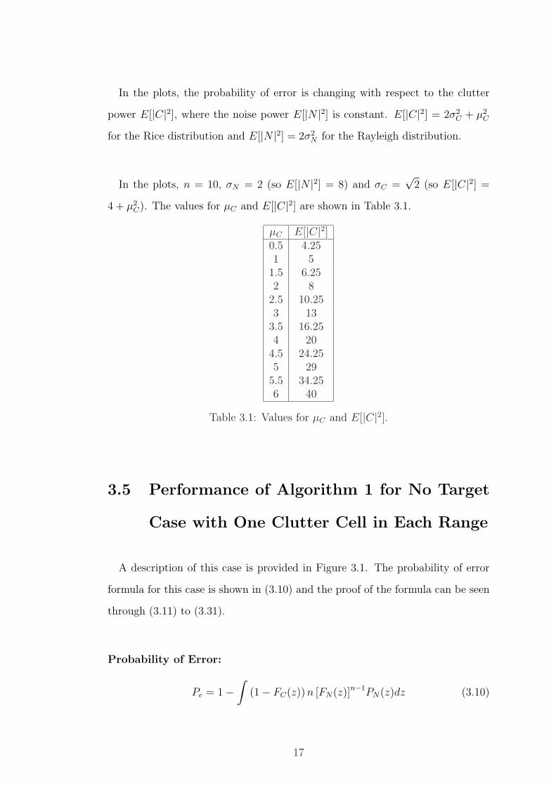
3.1 Description of Algorithm 1 for no target case with one clutter cell
in each range. . . . . . . . . . . . . . . . . . . . . . . . . . . . . . 18
3.2 Probability of error for Algorithm 1 for no target case with one
clutter cell in each range. . . . . . . . . . . . . . . . . . . . . . . . 20
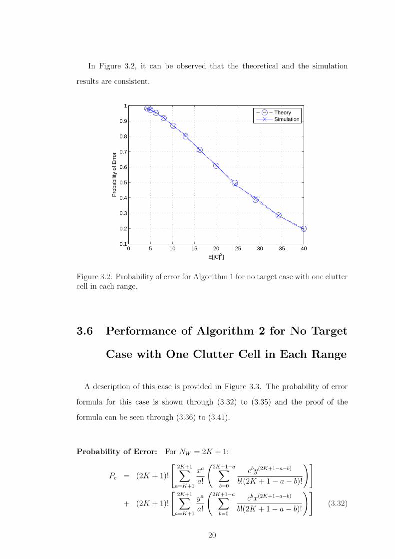
3.3 Description of Algorithm 2 for no target case with one clutter cell
in each range. . . . . . . . . . . . . . . . . . . . . . . . . . . . . . 21
3.4 Probability of error for Algorithm 2 for no target case with one
clutter cell in each range. . . . . . . . . . . . . . . . . . . . . . . . 24
xi

3.5 Comparing the effect of NW in probability of error for Algorithm
2 for no target case with one clutter cell in each range. . . . . . . 25
3.6 Comparing the probability of error for Algorithm 1 and Algorithm
2 for no target case with one clutter cell in each range. . . . . . . 26
3.7 Description of Algorithm 1 for no target case with two clutter cells
in each range. . . . . . . . . . . . . . . . . . . . . . . . . . . . . . 27
3.8 Probability of error for Algorithm 1 for no target case with two
clutter cells in each range. . . . . . . . . . . . . . . . . . . . . . . 28
3.9 Comparing the probability of error for Algorithm 1 for no target
case with one clutter cell and two clutter cells in each range. . . . 29
3.10 Comparing the probability of error for Algorithm 1 and Algorithm
2a for no target case with two clutter cells in each range. . . . . . 30
3.11 Comparing the probability of error for Algorithm 2a and Algo-
rithm 2b for no target case with two clutter cells in each range. . 31
3.12 Description of Algorithm 1 for one target case with one clutter
cell in each range. . . . . . . . . . . . . . . . . . . . . . . . . . . . 32
3.13 Probability of error for Algorithm 1 for one target case with one
clutter cell in each range. . . . . . . . . . . . . . . . . . . . . . . . 33
3.14 Description of Algorithm 1 for two target case with one clutter
cell in each range. . . . . . . . . . . . . . . . . . . . . . . . . . . . 34
3.15 Probability of error for Algorithm 1 for two target case with 1
clutter cell in each range. . . . . . . . . . . . . . . . . . . . . . . . 35
3.16 Description of Algorithm 1 for one target case with two clutter
cells in each range. . . . . . . . . . . . . . . . . . . . . . . . . . . 36
xii

3.17 Probability of error for Algorithm 1 for one target case with two
clutter cells in each range. . . . . . . . . . . . . . . . . . . . . . . 37
3.18 Description of Algorithm 2 for one target case with one clutter
cell in each range. . . . . . . . . . . . . . . . . . . . . . . . . . . . 38
3.19 Probability of error for Algorithm 2 for one target case with one
clutter cell in each range . . . . . . . . . . . . . . . . . . . . . . . 41
4.1 Detection signal for 90 degree azimuth angle. . . . . . . . . . . . . 44
4.2 Detection signal for 70 degree azimuth angle. . . . . . . . . . . . . 45
4.3 More noisy detection signal for 90 degree azimuth angle. . . . . . 46
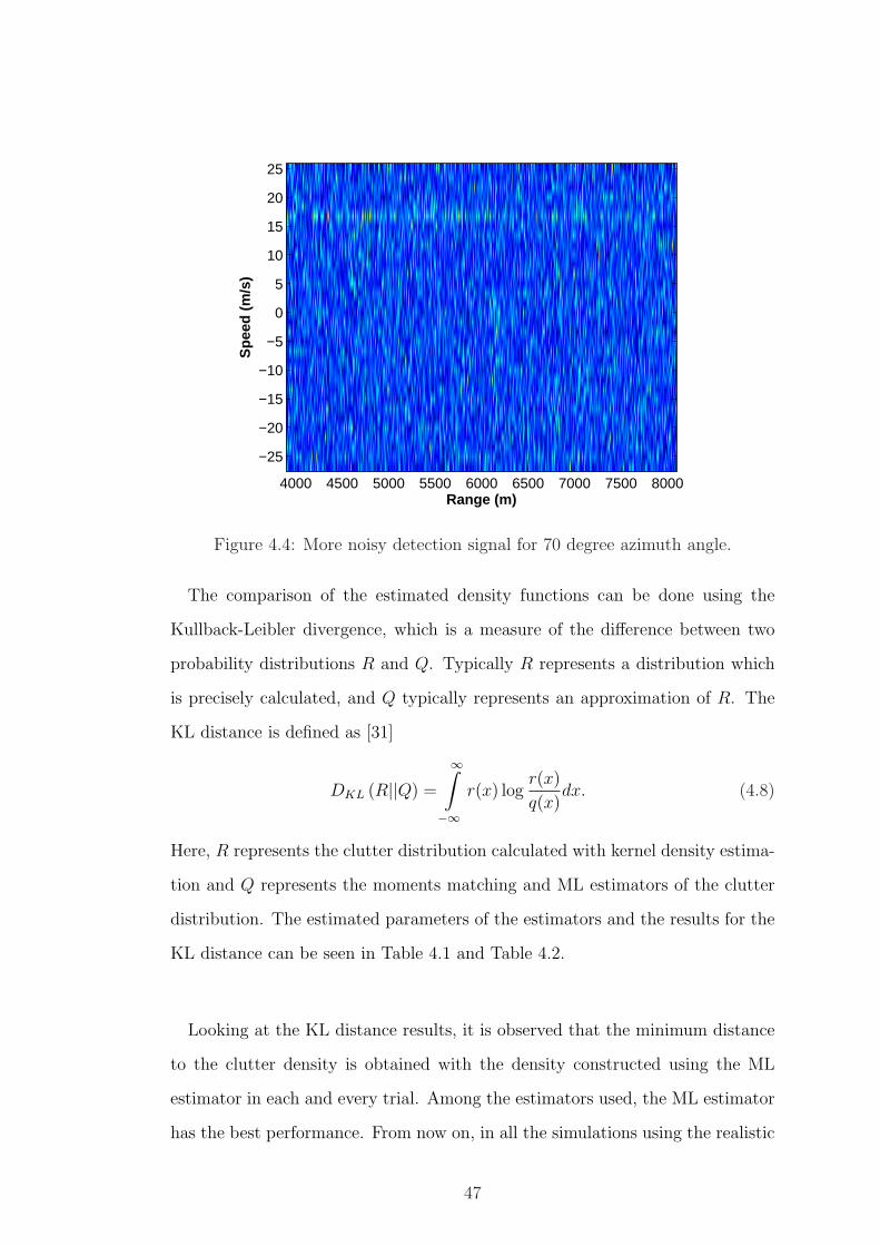
4.4 More noisy detection signal for 70 degree azimuth angle. . . . . . 47
4.5 Histogram of clutter for 90 degree azimuth angle. . . . . . . . . . 48
4.6 Histogram of clutter for 70 degree azimuth angle. . . . . . . . . . 49
4.7 Histogram of more noisy clutter for 90 degree azimuth angle. . . . 50
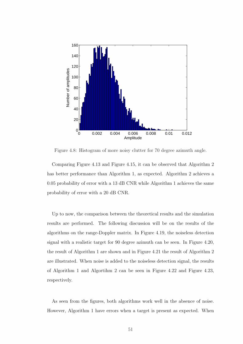
4.8 Histogram of more noisy clutter for 70 degree azimuth angle. . . . 51
4.9 Clutter pdf’s for different estimators for 90 degree azimuth. . . . . 52
4.10 Clutter pdf’s for different estimators for 70 degree azimuth. . . . . 53
4.11 More noisy clutter pdf’s for different estimators for 90 degree az-
imuth. . . . . . . . . . . . . . . . . . . . . . . . . . . . . . . . . . 53
4.12 More noisy clutter pdf’s for different estimators for 70 degree az-
imuth. . . . . . . . . . . . . . . . . . . . . . . . . . . . . . . . . . 54
xiii
4.13 Comparing the simulation results with theoretical results for no
target case using Algorithm 1 for 90 degree azimuth. . . . . . . . 54
4.14 Comparing the simulation results with theoretical results for no
target case using Algorithm 1 for 70 degree azimuth. . . . . . . . 55
4.15 Comparing the simulation results with theoretical results for no
target case using Algorithm 2 for 90 degree azimuth. . . . . . . . 55
4.16 Comparing the simulation results with theoretical results for no
target case using Algorithm 2 for 70 degree azimuth. . . . . . . . 56
4.17 Comparing the simulation results with theoretical results for one
point target case using Algorithm 1 for 90 degree azimuth. . . . . 56
4.18 Comparing the simulation results with theoretical results for one
point target case using Algorithm 1 for 70 degree azimuth. . . . . 57
4.19 Pure detection signal with a realistic target for 90 degree azimuth. 57
4.20 Detected clutter for 90 degree azimuth using Algorithm 1. . . . . 58
4.21 Detected clutter for 90 degree azimuth using Algorithm 2. . . . . 58
4.22 Detected clutter from noisy environment for 90 degree azimuth
using Algorithm 1. . . . . . . . . . . . . . . . . . . . . . . . . . . 59
4.23 Detected clutter from noisy environment for 90 degree azimuth
using Algorithm 2. . . . . . . . . . . . . . . . . . . . . . . . . . . 59
xiv
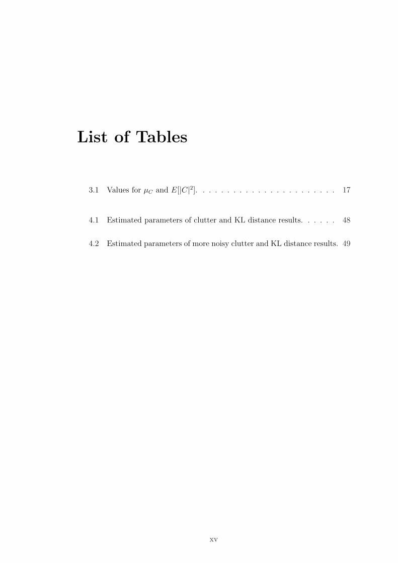
List of Tables
3.1 Values for µC and E[|C|2]. . . . . . . . . . . . . . . . . . . . . . . 17
4.1 Estimated parameters of clutter and KL distance results. . . . . . 48
4.2 Estimated parameters of more noisy clutter and KL distance results. 49
xv

To my family. . .

Chapter 1
INTRODUCTION
A wide spectrum of components ranging from defensive or offensive devices
to the strategic integration of more complex technologies designed to defeat an
enemy constitute weapons systems [4]. Weapon systems must be capable of ac-
complishing some functions like target detection, classification, localization and
tracking in order to destruct or neutralize the target. Countless target and envi-
ronmental characteristics including clutter location, target location, target speed
and target direction emerges a need for complex detection systems. Noise gener-
ated by the detection system itself complicates the target detection. Therefore,
appropriate design is needed to distinguish target signals from noise [4].
Radar is an acronym for Radio Detection and Ranging [5]-[8]. Some objects
can be detected and located at far greater distances than a naked eye can see,
using the applications of electromagnetic waves. This sensing is not affected by
most obstacles to ordinary vision like night, cloud, fog and smoke. In addition,
radar permits the accurate measurement of the range and velocity of what it
senses with a precision cannot be obtainable by a human operator. Some other
aspects of radar performance are poorer than that of the eye [4].
1
Pulse-Doppler radar systems are used in order to detect both locations and
radial velocities of the targets. Airborne pulse-Doppler radars are operating in
an environment being exposed to strong echoes reflected from the ground [9].
These reflections constitute clutter signals. Target detection in the presence of
clutter becomes difficult. An approach to detect targets includes finding the po-
sition of the clutter and then running different constant false alarm rate (CFAR)
algorithms in the clutter zone, in the vicinity of the clutter zone and in the far
field of the clutter zone.
In this thesis, we study the detection of clutter in the range-Doppler plane.
This plane is observed after the pulse-Doppler processing of the signals reflected
from the environment. In airborne pulse-Doppler radars, the clutter is always
present and some targets may also be present in the range-Doppler plane.
In most radar applications, clutter is eliminated instead of locating its position
in order to detect targets. However, this approach allows to detect moving targets
and it is called as moving target indication (MTI). Stationary targets are also
cancelled out with the clutter because they have a spectrum falling into the
clutter spectrum. Ground looking stationary radars are exposed to fixed ground
clutter which is around zero Doppler. In this way they distinguish the moving
targets. An airborne ground looking moving radar is also exposed to ground
clutter but in this case it is not fixed along the motion of the radar and it is not
always around the zero Doppler. Moving targets can also be detected in this case
because they have different spectra than the clutter [10]-[14]. In order to detect
the stationary targets, first the clutter should be detected because the desired
targets lie inside the clutter. When the clutter is detected, it is easy to find the
moving targets in the rest of the process. There are some approaches to find
the clutter position using the range-Doppler plane. Because this is a military
2
application, it is hard to find this type of techniques that are uncovered. Our
algorithms are useful to solve this problem.
In [15], an improved signal processing technique is presented. It is suitable for
airborne Doppler radars. The primary objective is to distinguish targets from
the mainbeam clutter. The technique does not require accurate measurements
of the velocity or the altitude of the moving radar platform [15]. After obtaining
the range-Doppler matrix, each cell of the matrix is compared to a scaled mean
of the background noise. If the value in the cell exceeds the threshold, a logic
one is set to that cell. If the value in the cell is lower than the threshold, a
logic zero is set to that cell. In the logic matrix, the clutter signals occur in
many contiguous cells and target signals are present in only a few isolated cells
or in a single cell [15]. The problem with this technique is the calculation of the
threshold value. It is the scaled mean of the background noise but the noise level
is not accurately known. For the case in which the noise is known accurately, it
is again not defined how the mean of the background noise is scaled.
In [16], a method for clutter detection is presented. In this technique, if a large
number of cells that have large amplitudes are present in a range, those cells are
identified as clutter. This procedure is repeated on each range cell. The problem
with the discussed method is that the word “large” is not defined accurately.
In [17], a new model to detect objects in a given image is proposed. The
model can detect objects, the boundaries of which are not necessarily defined by
gradient. It is used in radar imaging to reveal targets. In addition, this method
can be applied to the clutter detection problem. The range-Doppler matrix is
also an image. The edges of the clutter and targets can be detected. If there
is only clutter in the matrix, the result of this method gives the clutter edges.
However, if there are targets, in addition to the clutter, in the matrix, the result
3
of this method gives both the clutter and target edges and a further processing
is needed to distinguish the clutter from targets. Moreover, this technique is a
slow one because it is an iterative algorithm.
In our work, we propose two algorithms for clutter detection. The first one is
a simple and fast algorithm. The second one is a more complex and slower algo-
rithm. Simplicity of the first algorithm would cause a drop in the performance
for the sake of higher speed. The second one would have better performance in
a longer period of running time. Both algorithms are based on simple nonlin-
ear filters. They can be used to detect clutter regardless of its Doppler value.
Namely, clutter can be around zero Doppler or it can be around any other value
of Doppler frequency.
The first algorithm includes a single nonlinear filter. This filter selects the
maximum valued cell as the clutter cell in a range bin. It would have good
performance when the range-Doppler plane is exposed to low noise and no target
is present in the plane. When high noise or a target is present in the plane, the
algorithm would begin to give erronous results.
The second algorithm includes one more nonlinear filter. In addition to the
maximum selecting filter, a median filter is present. It filters the bin numbers of
the cells that are chosen as clutter by the first algorithm. The median filter used
here would apply a correction on the erronous results of the first algorithm. The
run time increases with the length of the median filter. For the longer lengths of
the median filter, the algorithm would give improved results.
In Chapter 2, the system model is introduced. The simulation environment
consists of a terrain model, a target model and a radar model. Each model is
discussed in detail in that chapter. The steps of the pulse-Doppler processing is
4

also mentioned. In Chapter 3, the clutter detection algorithms are explained in
detail. The probability of error formulas of the algorithms are obtained. More-
over, a series of performance analysis is conducted for some different cases. The
results of different cases are also compared in that chapter. In Chapter 4, sim-
ulation results on realistic clutter and target data are discussed. The results of
the algorithms on realistic scenarios are presented. The difference in the perfor-
mance of the algorithms can also be observed in that chapter. Finally, Chapter
5 concludes the thesis.
5
Chapter 2
SYSTEM MODEL
In this chapter, the radar system model is introduced in order to explain the
environment in which the clutter detection algorithms are run. First of all,
a terrain must be generated in order to simulate an air platform flying on the
terrain. The air platform carries a pulse-Doppler radar system on it. It transmits
the radar signal from a specified height and elevation for a 360-degree coverage
of azimuth and listens for the reflected signals from the terrain. The reflections
from the terrain constitute the raw clutter signal. After pulse-Doppler processing
of the received signals, the range-Doppler matrix is formed, which indicates the
Doppler and range of the clutter. In addition, realistic target models are used
in some simulations. The target is processed individually and then added to the
clutter signal.
2.1 Terrain Generation
In [1], some fractal terrain generating algorithms are discussed. The algorithms
consist of midpoint displacement in one dimension, height maps, triangular-edge
6
subdivision, diamond-square subdivision and square-square subdivision. A real-
istic terrain should not include creases and its roughness should be in accordance
with the real geography. Among the algorithms, the diamond-square subdivision
technique is used to generate the realistic terrain. It is an algorithm that pro-
duces realistic terrains and can easily be implemented [1].
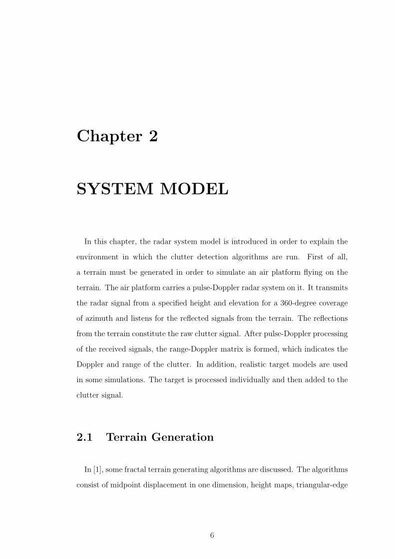
The diamond-square subdivision algorithm is divided into two stages as the
name implies: square stage and diamond stage. The process begins with a
square matrix. Some values should be assigned to the corners of the matrix
for the initiation of the process and then the subdivision begins [18], [19]. In
Figure 2.1(a), the blue point in the center is generated from the average of the
values initially generated,the remaining blue points, plus a random value. Now,
half diamonds are created. The red points in the same figure represents the
recently created points. They stay in the center of a full diamond. Their values
are the average of the points forming the diamond plus a random value. In
Figure 2.1(b), the blue points are coming from the previous stage and they form
squares. The recently created points are the red ones. They are in the center
of each square and their values are the average of the four values forming each
square plus a random value. In Figure 2.1(c), diamonds are formed again. The
iterations continue following this pattern until all the points in the matrix have
a value. The random numbers added should be selected from a reduced range
from iteration to iteration in order to get a smooth terrain. The other terrain
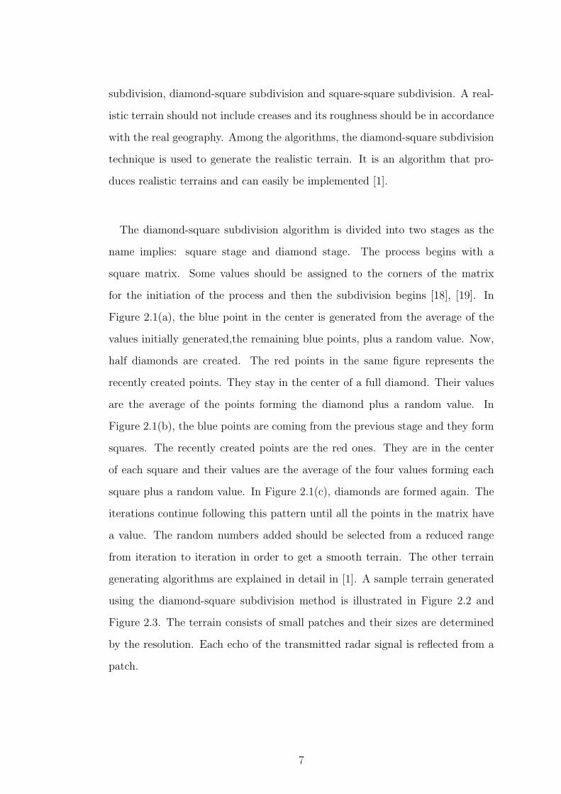
generating algorithms are explained in detail in [1]. A sample terrain generated
using the diamond-square subdivision method is illustrated in Figure 2.2 and
Figure 2.3. The terrain consists of small patches and their sizes are determined
by the resolution. Each echo of the transmitted radar signal is reflected from a
patch.
7
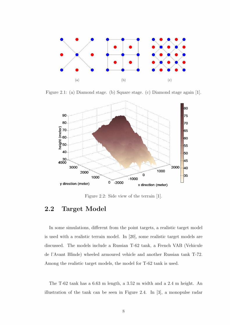
Figure 2.1: (a) Diamond stage. (b) Square stage. (c) Diamond stage again [1].
Figure 2.2: Side view of the terrain [1].
2.2 Target Model
In some simulations, different from the point targets, a realistic target model
is used with a realistic terrain model. In [20], some realistic target models are
discussed. The models include a Russian T-62 tank, a French VAB (Vehicule
de l’Avant Blinde) wheeled armoured vehicle and another Russian tank T-72.
Among the realistic target models, the model for T-62 tank is used.
The T-62 tank has a 6.63 m length, a 3.52 m width and a 2.4 m height. An
illustration of the tank can be seen in Figure 2.4. In [3], a monopulse radar
8
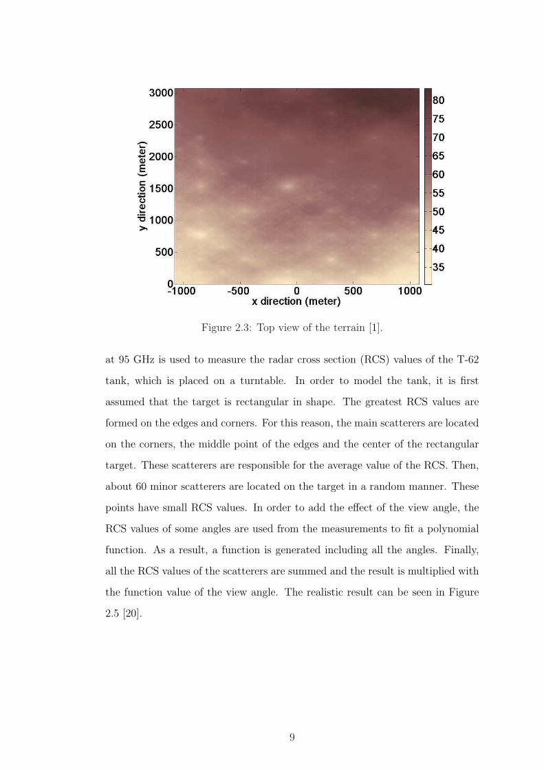
Figure 2.3: Top view of the terrain [1].
at 95 GHz is used to measure the radar cross section (RCS) values of the T-62
tank, which is placed on a turntable. In order to model the tank, it is first
assumed that the target is rectangular in shape. The greatest RCS values are
formed on the edges and corners. For this reason, the main scatterers are located
on the corners, the middle point of the edges and the center of the rectangular
target. These scatterers are responsible for the average value of the RCS. Then,
about 60 minor scatterers are located on the target in a random manner. These
points have small RCS values. In order to add the effect of the view angle, the
RCS values of some angles are used from the measurements to fit a polynomial
function. As a result, a function is generated including all the angles. Finally,
all the RCS values of the scatterers are summed and the result is multiplied with
the function value of the view angle. The realistic result can be seen in Figure
2.5 [20].
9

Figure 2.4: T-62 tank [2].
2.3 Radar Model and Pulse-Doppler Processing
After having a realistic terrain, a radar model which is mounted on an air
platform flying over the terrain is needed. The radar is modeled as a pulse-
Doppler radar because of the widespread use of it [9]. The generic radar waveform
and its complex envelope can be expressed in (2.1) and (2.2) respectively.
x(t) = a(t) ej[Ωt+θ(t)] (2.1)
x(t) = a(t) ejθ(t) (2.2)
where a(t) is the amplitude modulation of the radio frequency (RF) carrier, Ω
is the RF carrier frequency and θ(t) is the phase or frequency modulation of
the carrier [21]. Here, a(t) and θ(t) determines the type of the radar signal.
In a pulsed radar, a(t) has the form of a single pulse. However, for a better
Doppler resolution, pulse burst waveforms must be used [22]-[25]. Accordingly,
a(t) has the form of a sum of shifted pulses. In a pulse burst radar system using a
single antenna for transmission and reception, listening for the echoes continues
when a(t) is zero. Otherwise, transmission is performed. The phase or frequency
modulation, θ(t), allows a better range resolution than an unmodulated signal
10
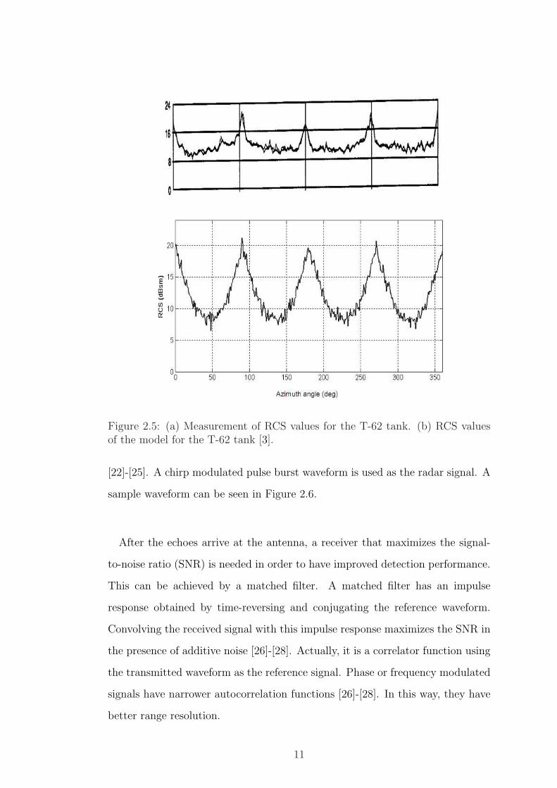
Figure 2.5: (a) Measurement of RCS values for the T-62 tank. (b) RCS valuesof the model for the T-62 tank [3].
[22]-[25]. A chirp modulated pulse burst waveform is used as the radar signal. A
sample waveform can be seen in Figure 2.6.
After the echoes arrive at the antenna, a receiver that maximizes the signal-
to-noise ratio (SNR) is needed in order to have improved detection performance.
This can be achieved by a matched filter. A matched filter has an impulse
response obtained by time-reversing and conjugating the reference waveform.
Convolving the received signal with this impulse response maximizes the SNR in
the presence of additive noise [26]-[28]. Actually, it is a correlator function using
the transmitted waveform as the reference signal. Phase or frequency modulated
signals have narrower autocorrelation functions [26]-[28]. In this way, they have
better range resolution.
11
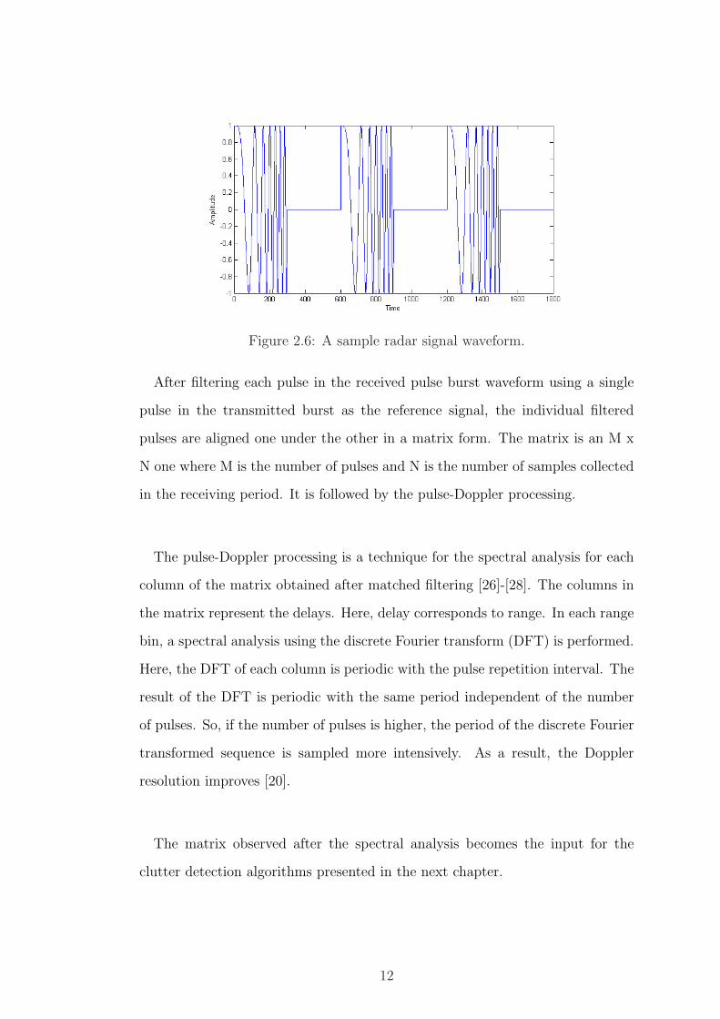
Figure 2.6: A sample radar signal waveform.
After filtering each pulse in the received pulse burst waveform using a single
pulse in the transmitted burst as the reference signal, the individual filtered
pulses are aligned one under the other in a matrix form. The matrix is an M x
N one where M is the number of pulses and N is the number of samples collected
in the receiving period. It is followed by the pulse-Doppler processing.
The pulse-Doppler processing is a technique for the spectral analysis for each
column of the matrix obtained after matched filtering [26]-[28]. The columns in
the matrix represent the delays. Here, delay corresponds to range. In each range
bin, a spectral analysis using the discrete Fourier transform (DFT) is performed.
Here, the DFT of each column is periodic with the pulse repetition interval. The
result of the DFT is periodic with the same period independent of the number
of pulses. So, if the number of pulses is higher, the period of the discrete Fourier
transformed sequence is sampled more intensively. As a result, the Doppler
resolution improves [20].
The matrix observed after the spectral analysis becomes the input for the
clutter detection algorithms presented in the next chapter.
12

Chapter 3
CLUTTER DETECTION
ALGORTIHMS AND
PERFORMANCE ANALYSIS
In this chapter, two clutter detection algorithms are presented. Notation and
assumptions used in performance analysis are explained. After getting the the-
oretical probability of error formulas for each case, they are compared with al-
gorithms’ performances on synthetically generated data using point targets in
some cases. Performances of the algorithms are also compared with each other.
3.1 Notation
Here, the notation used in the analysis will be described. A(r, ν) is the range-
Doppler matrix where r is the range index and ν is the Doppler frequency, PC(·)is the probability density function (p.d.f.) of the clutter, PT (·) is the p.d.f. of
the target, PN(·) is the p.d.f. of the noise, FC(·) is the cumulative distribution
function (c.d.f.) of the clutter, FT (·) is the c.d.f. of the target, FN(·) is the c.d.f.
13

of the noise, n is the number of noise bins in each range cell, and NW is the
median filter length which is used in Algorithm 2 in Section 3.3.
3.2 Assumptions
Here, the assumptions made in the analysis will be described. Noise cells are
assumed to be independent and identically distributed (i.i.d.) which is consistent
with the realistic case. Clutter cells are assumed to be i.i.d. This assumption
may not be true in the realistic case. It has no effect on Algorithm 1 because each
range cell is treated separately. However in Algorithm 2, this assumption leads
to approximate results in the analysis. When more than one clutter cells are
present in range cells, this assumption results in an approximation for Algorithm
1 as well.
3.3 Clutter Detection Algorithms
The algorithms will be described here are mainly developed for radars having
low Doppler resolution or clutter having low Doppler spread. Namely, the algo-
rithms are designed for detecting clutter which is present only in one Doppler
bin in each range cell in the range-Doppler matrix. The algorithms are described
as follows:
Algorithm 1:
Cr = arg maxν|A(r, ν)|, r = 1, 2, ... (3.1)
where Cr denotes the index of the clutter in the rth range cell.
14
In this algorithm, along each range cell the maximum valued bin is selected
as the clutter bin. Noise and targets may cause errors in the detection of the
clutter. This algorithm runs a single nonlinear filter. So, it is expected to run
faster than Algorithm 2 because it runs two nonlinear filters as follows:
Algorithm 2. Find f(r, i)’s and apply a nonlinear ordered statistics filter (me-
dian filter with filter length NW ). Namely,
f(r, i) = arg maxν|A(r + i, ν)| (3.2)
Cr = medianf(r,−j), ..., f(r, 0), ..., f(r, j), r = 1, 2, ... (3.3)
where j = NW−12
, f(r, i) denotes the index of the maximum Doppler frequency
bin in (r + i)th range cell, and Cr denotes the index of the clutter in the rth range
cell.
In this algorithm, a further step is included. After deciding the maximum
valued bins in each range cell, a median filter of length NW is applied to correct
any errors that are caused because of noise and targets. The level of the correction
depends on the median filter length NW . Running two nonlinear filters, this
algorithm is expected to run slower than Algorithm 1. However, it is expected
that there may also be performance difference in the algorithms. This will be
investigated in the following sections.
As mentioned before, the algorithms are designed for detecting the clutter,
which is present only in one Doppler bin in each range cell. The algorithms
can be further modified to detect clutters which can be present in more than
one Doppler bin in each range cell. For a clutter present in two Doppler cells,
Algorithm 1 can again run a nonlinear filter but this time it decides the maximum
and the second biggest valued bins as clutters. Similarly, Algorithm 2 can use
the results obtained from Algorithm 1 and can again run a median filter. In
15
Algorithm 2, there may be two approaches for this case, which will be reviewed
in a non-theoretical manner.
3.4 Performance
In the performance analysis, the clutter and the target cells are modeled to
have the Rice distribution and the noise has the Rayleigh distribution. The error
probabilities of the clutter detection for both algorithms will be calculated. Then
the theoretical and simulation results will be compared to investigate whether
they are consistent. P.d.f.s and c.d.f.s for clutter, target and noise are as follows:
The p.d.f. for the clutter is given by
PC(z) =z
σ2C
exp
(−(z2 + µ2C)
2σ2C
)I0
(zµ
σ2C
)(3.4)
where I0 is the modified Bessel funciton of the first kind with order zero, and the
corresponding c.d.f. is
FC(z) = 1−Q1
(µC
σC
,z
σC
)(3.5)
where Q1 is the Marcum Q-function.
The p.d.f. for the target is
PT (z) =z
σ2T
exp
(−(z2 + µ2T )
2σ2T
)I0
(zµ
σ2T
)(3.6)
where I0 is the modified Bessel funciton of the first kind with order zero, and the
corresponding c.d.f. is given by
FT (z) = 1−Q1
(µT
σT
,z
σT
)(3.7)
where Q1 is the Marcum Q-function.
The p.d.f. for the noise is expressed as
PN(z) =z
σ2N
e−z2/2σ2N (3.8)
and the corresponding c.d.f. is
FN(z) = 1− e−z2/2σ2N . (3.9)
16
In the plots, the probability of error is changing with respect to the clutter
power E[|C|2], where the noise power E[|N |2] is constant. E[|C|2] = 2σ2C + µ2
C
for the Rice distribution and E[|N |2] = 2σ2N for the Rayleigh distribution.
In the plots, n = 10, σN = 2 (so E[|N |2] = 8) and σC =√
2 (so E[|C|2] =
4 + µ2C). The values for µC and E[|C|2] are shown in Table 3.1.
µC E[|C|2]0.5 4.251 5
1.5 6.252 8
2.5 10.253 13
3.5 16.254 20
4.5 24.255 29
5.5 34.256 40
Table 3.1: Values for µC and E[|C|2].
3.5 Performance of Algorithm 1 for No Target
Case with One Clutter Cell in Each Range
A description of this case is provided in Figure 3.1. The probability of error
formula for this case is shown in (3.10) and the proof of the formula can be seen
through (3.11) to (3.31).
Probability of Error:
Pe = 1−∫
(1− FC(z)) n [FN(z)]n−1PN(z)dz (3.10)
17
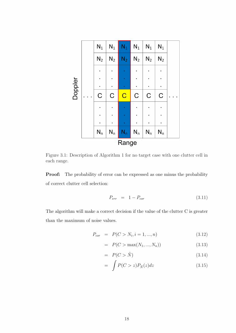
Figure 3.1: Description of Algorithm 1 for no target case with one clutter cell ineach range.
Proof: The probability of error can be expressed as one minus the probability
of correct clutter cell selection:
Perr = 1− Pcor (3.11)
The algorithm will make a correct decision if the value of the clutter C is greater
than the maximum of noise values.
Pcor = P (C > Ni, i = 1, ..., n) (3.12)
= P (C > max(N1, ..., Nn)) (3.13)
= P (C > N) (3.14)
=
∫P (C > z)PN(z)dz (3.15)
18

where N∆= max(N1, ..., Nn) and N ′
is are i.i.d. Then, the cdf of N is obtained as
follows:
FN(z) = P (N < z) (3.16)
= P (max(N1, ..., Nn) < z) (3.17)
= P (N1 < z, ..., Nn < z) (3.18)
N′is being independent,
= P (N1 < z)...P (Nn < z) (3.19)
N′is being identical,
= [P (N1 < z)]n (3.20)
= [FN1(z)]n (3.21)
The p.d.f. of N is given by
PN(z) =d
dzFN(z) (3.22)
=d
dz[FN1(z)]n (3.23)
= n[FN1(z)]n−1 d
dzFN1(z) (3.24)
= n[FN1(z)]n−1PN1(z) (3.25)
The last unknown in the probability of correct clutter cell selection equation is
expressed as
P (C > z) = 1− P (C ≤ z) (3.26)
= 1− FC(z) (3.27)
The probability of correct clutter cell selection is
Pcor = P (C > N) (3.28)
=
∫(1− FC(z)) n [FN1(z)]n−1PN1(z)dz (3.29)
Finally, the probability of error is given by
Perr = 1− Pcor (3.30)
= 1−∫
(1− FC(z)) n [FN1(z)]n−1PN1(z)dz (3.31)
19
In Figure 3.2, it can be observed that the theoretical and the simulation
results are consistent.
0 5 10 15 20 25 30 35 400.1
0.2
0.3
0.4
0.5
0.6
0.7
0.8
0.9
1
E[|C|2]
Pro
babi
lity
of E
rror
TheorySimulation
Figure 3.2: Probability of error for Algorithm 1 for no target case with one cluttercell in each range.
3.6 Performance of Algorithm 2 for No Target
Case with One Clutter Cell in Each Range
A description of this case is provided in Figure 3.3. The probability of error
formula for this case is shown through (3.32) to (3.35) and the proof of the
formula can be seen through (3.36) to (3.41).
Probability of Error: For NW = 2K + 1:
Pe = (2K + 1)!
[2K+1∑
a=K+1
xa
a!
(2K+1−a∑
b=0
cby(2K+1−a−b)
b!(2K + 1− a− b)!
)]
+ (2K + 1)!
[2K+1∑
a=K+1
ya
a!
(2K+1−a∑
b=0
cbx(2K+1−a−b)
b!(2K + 1− a− b)!
)](3.32)
20
Figure 3.3: Description of Algorithm 2 for no target case with one clutter cell ineach range.
where c is the correct decision probability for clutter position, x is the probability
of deciding a bin that is above the clutter bin and y is the probability of deciding
a bin that is below the clutter bin in each range. Namely,
c =
∫(1− FC(z)) n [FN(z)]n−1PN(z)dz (3.33)
x = (1− c)ε (3.34)
y = (1− c)(1− ε) (3.35)
where ε = 12
in the case of the clutter that is in the middle of each range cell.
Actually, it is the ratio of the number of noise bins lying above the clutter bin
to the total number of noise bins.
Proof: The median filter length is NW = 2K + 1. If the number of bins lying
above the clutter bin, namely x’s, in the median window are more than K, the
median filter results in an error. Similarly, if the number of bins lying below the
clutter bin, namely y’s, in the median window are more than K, the median filter
21
result is again an error. To illustrate, consider a median window with length 3.
There are x, c and y values in this window. To have the result to be an error, the
following ordered combinations should occur in the window: xxc, xxx, cyy, yyy.
Note that the given combinations are ordered sets. The median filter orders its
inputs and gives the one in the middle as the output. Therefore, the sets do not
have to be in an ordered form. Their unordered combinations have to be taken
into account. All of these requirements lead to the following proof for the generic
case:
Pe = Pex + Pey (3.36)
where
Pex =(2K + 1)!
(K + 1)!xK+1
K∑a=0
cay(K−a)
a!(K − a)!
+(2K + 1)!
(K + 2)!xK+2
K−1∑a=0
cay(K−1−a)
a!(K − 1− a)!
+ ...
+(2K + 1)!
(2K + 1)!x2K+1
0∑a=0
cay(0−a)
a!(0− a)!. (3.37)
After arranging the above equation, it reduces to the following equation:
Pex = (2K + 1)!
[2K+1∑
a=K+1
xa
a!
(2K+1−a∑
b=0
cby(2K+1−a−b)
b!(2K + 1− a− b)!
)]. (3.38)
Similarly,
Pey =(2K + 1)!
(K + 1)!yK+1
K∑a=0
cax(K−a)
a!(K − a)!
+(2K + 1)!
(K + 2)!yK+2
K−1∑a=0
cax(K−1−a)
a!(K − 1− a)!
+ ...
+(2K + 1)!
(2K + 1)!y2K+1
0∑a=0
cax(0−a)
a!(0− a)!. (3.39)
After arranging the above equation, it reduces to the following equation:
Pey = (2K + 1)!
[2K+1∑
a=K+1
ya
a!
(2K+1−a∑
b=0
cbx(2K+1−a−b)
b!(2K + 1− a− b)!
)]. (3.40)
22

Combining the above equations, the resulting equation is as follows:
Pe = (2K + 1)!
[2K+1∑
a=K+1
xa
a!
(2K+1−a∑
b=0
cby(2K+1−a−b)
b!(2K + 1− a− b)!
)]
+ (2K + 1)!
[2K+1∑
a=K+1
ya
a!
(2K+1−a∑
b=0
cbx(2K+1−a−b)
b!(2K + 1− a− b)!
)]. (3.41)
In Figure 3.4 it can be observed that the theoretical and the simulation results
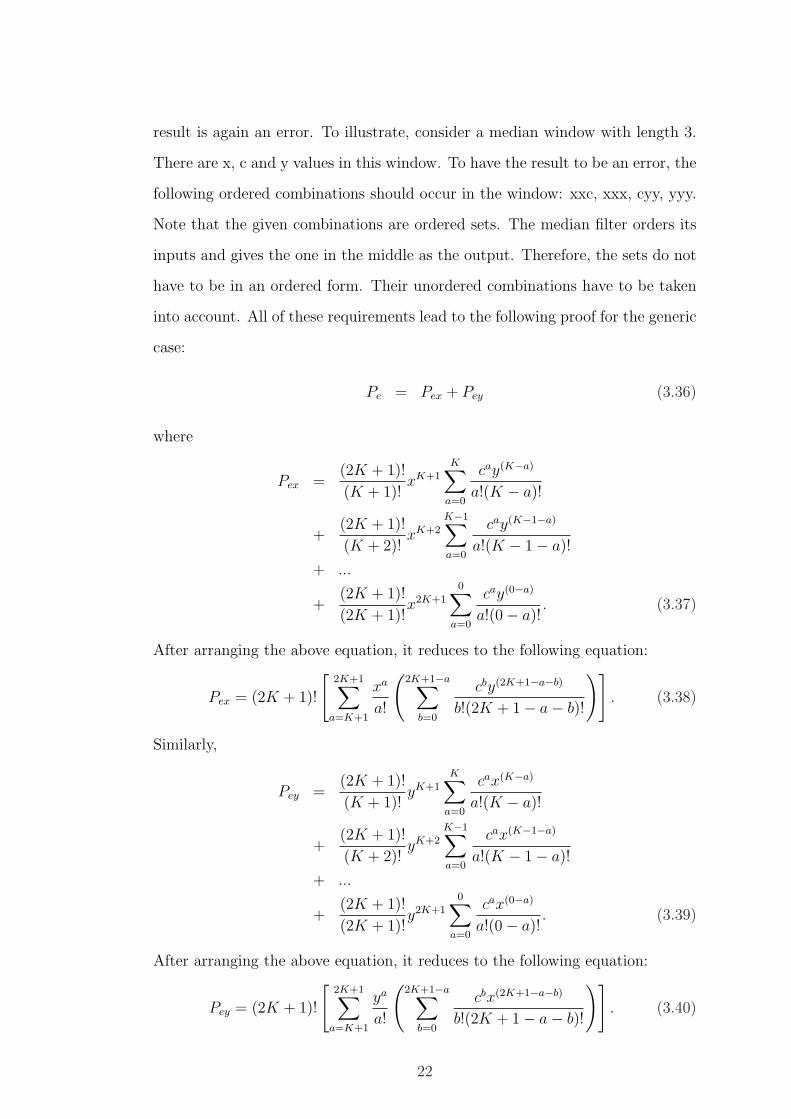
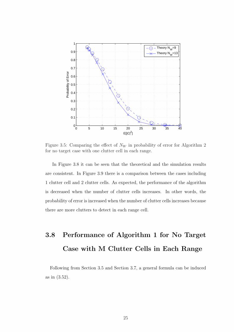
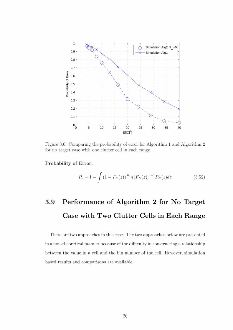
are consistent. In Figure 3.5 the effect of the median filter length can be seen.
When the length of the filter is increased, the performance of the algorithm
is also increased. In other words, the probability of error decreases with the
increase in the median filter length. In Figure 3.6 the performance difference
between the two algorithms can be observed. Expectedly, the performance of
Algorithm 2 is better than that of Algorithm 1. Even with a small window
length, the probability of error of Algorithm 2 is less than the probability of
error of Algorithm 1 because Algorithm 2 uses more data to decide the position
of the clutter. In other words, Algorithm 2 achieves a lower probability of error
for a given clutter power, or equivalently requires a lower power of clutter for a
specific probability of error compared to Algorithm 1.
3.7 Performance of Algorithm 1 for No Target
Case with Two Clutter Cells in Each Range
A description of this case is provided in Figure 3.7. The probability of error
formula for this case is shown in (3.42) and the proof of the formula can be seen
through (3.43) to (3.51).
Probability of Error:
Pe = 1−∫
(1− FC(z))2 n [FN(z)]n−1PN(z)dz (3.42)
23
0 5 10 15 20 25 30 35 400
0.1
0.2
0.3
0.4
0.5
0.6
0.7
0.8
0.9
1
E[|C|2]
Pro
babi
lity
of E
rror
SimulationTheory
Figure 3.4: Probability of error for Algorithm 2 for no target case with one cluttercell in each range.
Proof:
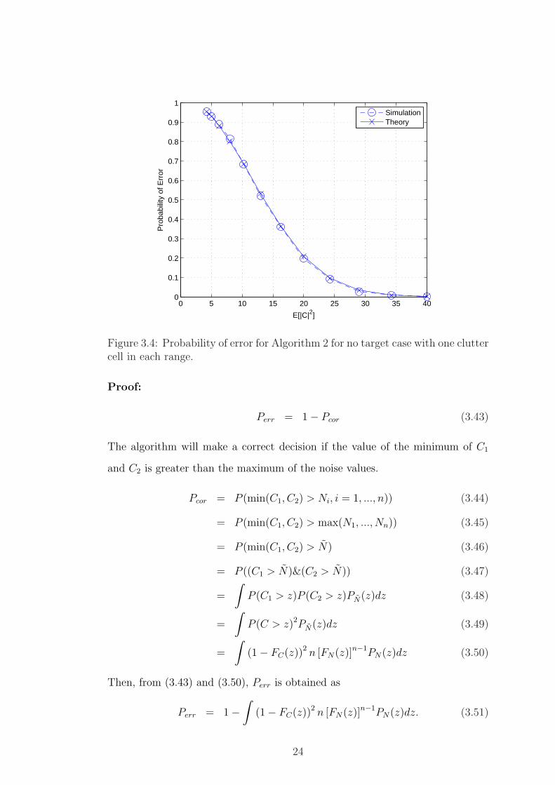
Perr = 1− Pcor (3.43)
The algorithm will make a correct decision if the value of the minimum of C1
and C2 is greater than the maximum of the noise values.
Pcor = P (min(C1, C2) > Ni, i = 1, ..., n)) (3.44)
= P (min(C1, C2) > max(N1, ..., Nn)) (3.45)
= P (min(C1, C2) > N) (3.46)
= P ((C1 > N)&(C2 > N)) (3.47)
=
∫P (C1 > z)P (C2 > z)PN(z)dz (3.48)
=
∫P (C > z)2PN(z)dz (3.49)
=
∫(1− FC(z))2 n [FN(z)]n−1PN(z)dz (3.50)
Then, from (3.43) and (3.50), Perr is obtained as
Perr = 1−∫
(1− FC(z))2 n [FN(z)]n−1PN(z)dz. (3.51)
24
0 5 10 15 20 25 30 35 400
0.1
0.2
0.3
0.4
0.5
0.6
0.7
0.8
0.9
1
E[|C|2]
Pro
babi
lity
of E
rror
Theory N
W=9
Theory NW
=13
Figure 3.5: Comparing the effect of NW in probability of error for Algorithm 2for no target case with one clutter cell in each range.
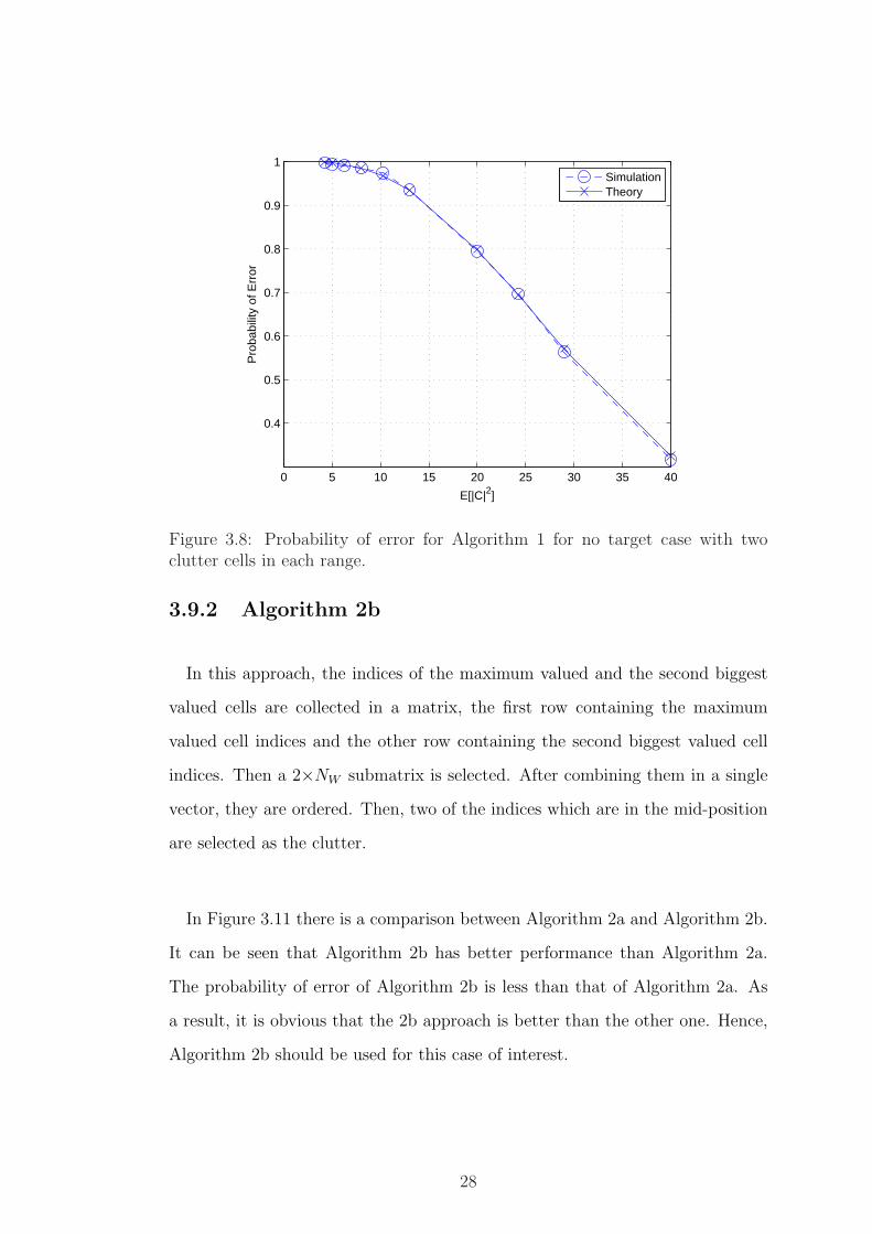
In Figure 3.8 it can be seen that the theoretical and the simulation results
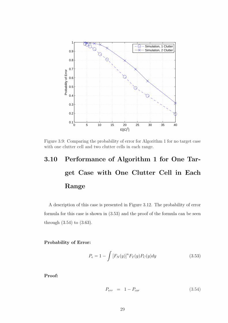
are consistent. In Figure 3.9 there is a comparison between the cases including
1 clutter cell and 2 clutter cells. As expected, the performance of the algorithm
is decreased when the number of clutter cells increases. In other words, the
probability of error is increased when the number of clutter cells increases because
there are more clutters to detect in each range cell.
3.8 Performance of Algorithm 1 for No Target
Case with M Clutter Cells in Each Range
Following from Section 3.5 and Section 3.7, a general formula can be induced
as in (3.52).
25
0 5 10 15 20 25 30 35 400
0.1
0.2
0.3
0.4
0.5
0.6
0.7
0.8
0.9
1
E[|C|2]
Pro
babi
lity
of E
rror
Simulation Alg2 N
W=5
Simulation Alg1
Figure 3.6: Comparing the probability of error for Algorithm 1 and Algorithm 2for no target case with one clutter cell in each range.
Probability of Error:
Pe = 1−∫
(1− FC(z))M n [FN(z)]n−1PN(z)dz (3.52)
3.9 Performance of Algorithm 2 for No Target
Case with Two Clutter Cells in Each Range
There are two approaches in this case. The two approaches below are presented
in a non-theoretical manner because of the difficulty in constructing a relationship
between the value in a cell and the bin number of the cell. However, simulation
based results and comparisons are available.
26
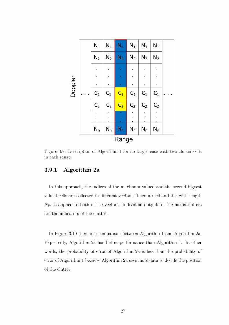
Figure 3.7: Description of Algorithm 1 for no target case with two clutter cellsin each range.
3.9.1 Algorithm 2a
In this approach, the indices of the maximum valued and the second biggest
valued cells are collected in different vectors. Then a median filter with length
NW is applied to both of the vectors. Individual outputs of the median filters
are the indicators of the clutter.
In Figure 3.10 there is a comparison between Algorithm 1 and Algorithm 2a.
Expectedly, Algorithm 2a has better performance than Algorithm 1. In other
words, the probability of error of Algorithm 2a is less than the probability of
error of Algorithm 1 because Algorithm 2a uses more data to decide the position
of the clutter.
27
0 5 10 15 20 25 30 35 40
0.4
0.5
0.6
0.7
0.8
0.9
1
E[|C|2]
Pro
babi
lity
of E
rror
SimulationTheory
Figure 3.8: Probability of error for Algorithm 1 for no target case with twoclutter cells in each range.
3.9.2 Algorithm 2b
In this approach, the indices of the maximum valued and the second biggest
valued cells are collected in a matrix, the first row containing the maximum
valued cell indices and the other row containing the second biggest valued cell
indices. Then a 2×NW submatrix is selected. After combining them in a single
vector, they are ordered. Then, two of the indices which are in the mid-position
are selected as the clutter.
In Figure 3.11 there is a comparison between Algorithm 2a and Algorithm 2b.
It can be seen that Algorithm 2b has better performance than Algorithm 2a.
The probability of error of Algorithm 2b is less than that of Algorithm 2a. As
a result, it is obvious that the 2b approach is better than the other one. Hence,
Algorithm 2b should be used for this case of interest.
28
0 5 10 15 20 25 30 35 400.1
0.2
0.3
0.4
0.5
0.6
0.7
0.8
0.9
1
E[|C|2]
Pro
babi
lity
of E
rror
Simulation, 1 ClutterSimulation, 2 Clutter
Figure 3.9: Comparing the probability of error for Algorithm 1 for no target casewith one clutter cell and two clutter cells in each range.
3.10 Performance of Algorithm 1 for One Tar-
get Case with One Clutter Cell in Each
Range
A description of this case is presented in Figure 3.12. The probability of error
formula for this case is shown in (3.53) and the proof of the formula can be seen
through (3.54) to (3.63).
Probability of Error:
Pe = 1−∫
[FN(y)]nFT (y)PC(y)dy (3.53)
Proof:
Perr = 1− Pcor (3.54)
29
0 5 10 15 20 25 30 35 400
0.1
0.2
0.3
0.4
0.5
0.6
0.7
0.8
0.9
1
E[|C|2]
Pro
babi
lity
of E
rror
Alg2a Sim. N
W=5, 2 Clutter
Alg1 Simulation, 2 Clutter
Figure 3.10: Comparing the probability of error for Algorithm 1 and Algorithm2a for no target case with two clutter cells in each range.
The algorithm will make a correct decision if the value of C is greater than the
maximum of the noise values and the value of the point target.
Pcor = P ((C > Ni, i = 1, ..., n)&(C > T )) (3.55)
= P ((C > max(N1, ..., Nn))&(C > T )) (3.56)
= P ((C > N)&(C > T )) (3.57)
=
∫P (N < y)P (T < y)PC(y)dy (3.58)
=
∫FN(y)FT (y)PC(y)dy (3.59)
=
∫[FN(y)]nFT (y)PC(y)dy (3.60)
Pcor =
∫[FN(y)]nFT (y)PC(y)dy (3.61)
Perr = 1− Pcor (3.62)
Perr = 1−∫
[FN(y)]nFT (y)PC(y)dy (3.63)
30
0 5 10 15 20 25 30 35 400
0.1
0.2
0.3
0.4
0.5
0.6
0.7
0.8
0.9
1
E[|C|2]
Pro
babi
lity
of E
rror
Alg2a Simulation N
W=5
Alg2b Simulation NW
=5
Figure 3.11: Comparing the probability of error for Algorithm 2a and Algorithm2b for no target case with two clutter cells in each range.
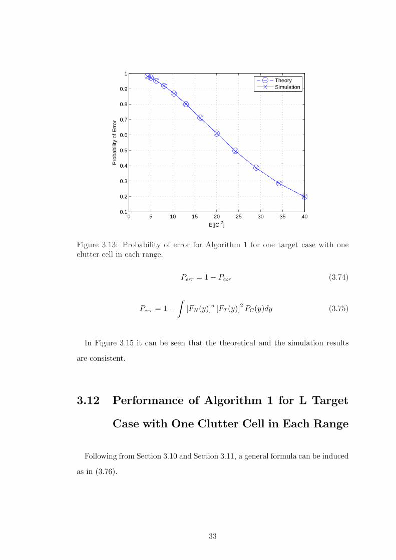
In Figure 3.13 it can be seen that the theoretical and the simulation results
are consistent.
3.11 Performance of Algorithm 1 for Two Tar-
get Case with One Clutter Cell in Each
Range
A description of this case is presented in Figure 3.14. The probability of error
formula for this case is shown in (3.64) and the proof of the formula can be seen
through (3.65) to (3.75).
Probability of Error:
Pe = 1−∫
[FN(y)]n[FT (y)]2PC(y)dy (3.64)
31
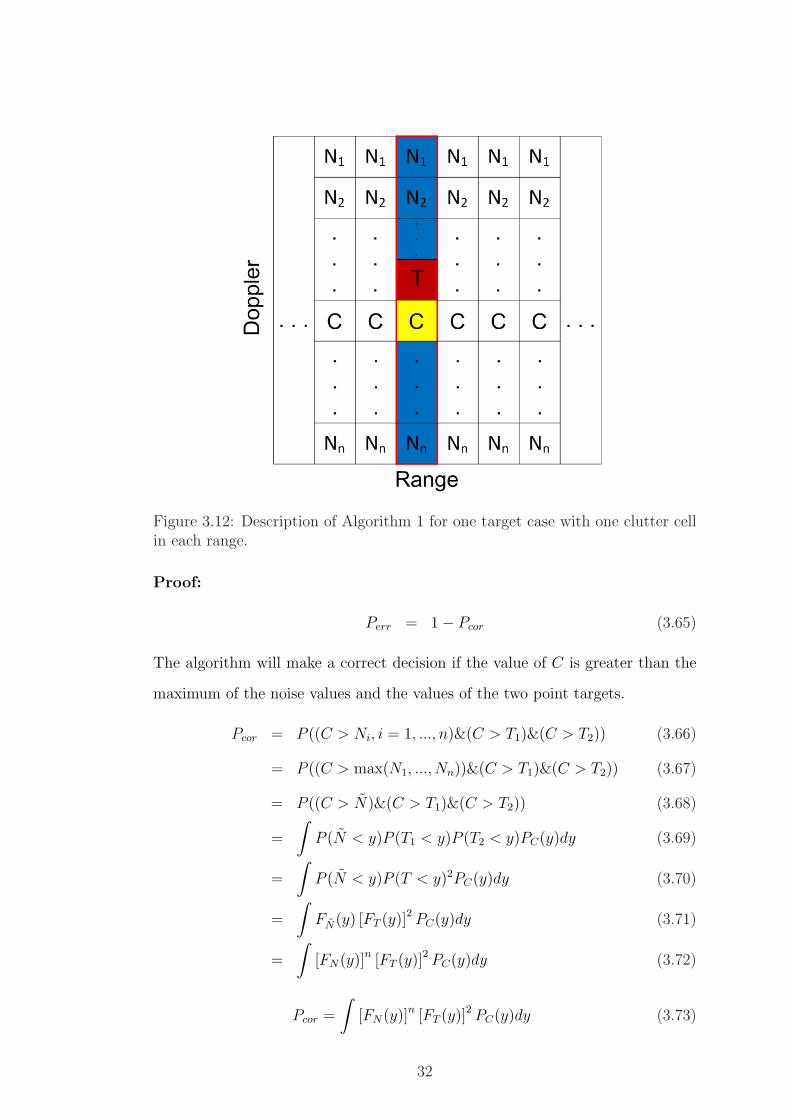
Figure 3.12: Description of Algorithm 1 for one target case with one clutter cellin each range.
Proof:
Perr = 1− Pcor (3.65)
The algorithm will make a correct decision if the value of C is greater than the
maximum of the noise values and the values of the two point targets.
Pcor = P ((C > Ni, i = 1, ..., n)&(C > T1)&(C > T2)) (3.66)
= P ((C > max(N1, ..., Nn))&(C > T1)&(C > T2)) (3.67)
= P ((C > N)&(C > T1)&(C > T2)) (3.68)
=
∫P (N < y)P (T1 < y)P (T2 < y)PC(y)dy (3.69)
=
∫P (N < y)P (T < y)2PC(y)dy (3.70)
=
∫FN(y) [FT (y)]2 PC(y)dy (3.71)
=
∫[FN(y)]n [FT (y)]2 PC(y)dy (3.72)
Pcor =
∫[FN(y)]n [FT (y)]2 PC(y)dy (3.73)
32
0 5 10 15 20 25 30 35 400.1
0.2
0.3
0.4
0.5
0.6
0.7
0.8
0.9
1
E[|C|2]
Pro
babi
lity
of E
rror
TheorySimulation
Figure 3.13: Probability of error for Algorithm 1 for one target case with oneclutter cell in each range.
Perr = 1− Pcor (3.74)
Perr = 1−∫
[FN(y)]n [FT (y)]2 PC(y)dy (3.75)
In Figure 3.15 it can be seen that the theoretical and the simulation results
are consistent.
3.12 Performance of Algorithm 1 for L Target
Case with One Clutter Cell in Each Range
Following from Section 3.10 and Section 3.11, a general formula can be induced
as in (3.76).
33
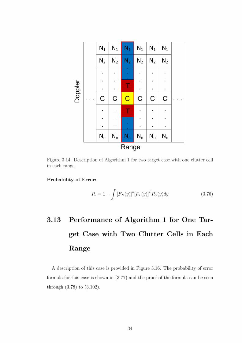
Figure 3.14: Description of Algorithm 1 for two target case with one clutter cellin each range.
Probability of Error:
Pe = 1−∫
[FN(y)]n[FT (y)]LPC(y)dy (3.76)
3.13 Performance of Algorithm 1 for One Tar-
get Case with Two Clutter Cells in Each
Range
A description of this case is provided in Figure 3.16. The probability of error
formula for this case is shown in (3.77) and the proof of the formula can be seen
through (3.78) to (3.102).
34

0 5 10 15 20 25 30 35 400.1
0.2
0.3
0.4
0.5
0.6
0.7
0.8
0.9
1
E[|C|2]
Pro
babi
lity
of E
rror
TheorySimulation
Figure 3.15: Probability of error for Algorithm 1 for two target case with 1 cluttercell in each range.
Probability of Error:
Pe = 1−∫
[FN(y)]nFT (y) [2PC(y)− 2FC(y)PC(y)] dy (3.77)
Proof:
Perr = 1− Pcor (3.78)
The algorithm will make a correct decision if the value of the minimum of C1 and
C2 is greater than the maximum of the noise values and the value of the point
target.
Pcor = P ((min(C1, C2) > Ni, i = 1, ..., n)&(min(C1, C2) > T )) (3.79)
= P ((min(C1, C2) > max(N1, ..., Nn))&(min(C1, C2) > T )) (3.80)
= P ((min(C1, C2) > N)&(min(C1, C2) > T )) (3.81)
= P ((C2 > N)&(C2 > T )) (3.82)
=
∫P (N < y)P (T < y)PC2
(y)dy (3.83)
35
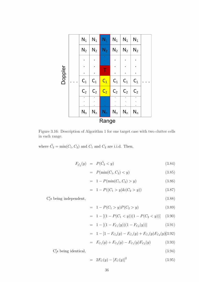
Figure 3.16: Description of Algorithm 1 for one target case with two clutter cellsin each range.
where C2 = min(C1, C2) and C1 and C2 are i.i.d. Then,
FC2(y) = P (C2 < y) (3.84)
= P (min(C1, C2) < y) (3.85)
= 1− P (min(C1, C2) > y) (3.86)
= 1− P ((C1 > y)&(C2 > y)) (3.87)
C′is being independent, (3.88)
= 1− P (C1 > y)P (C2 > y) (3.89)
= 1− [(1− P (C1 < y))(1− P (C2 < y))] (3.90)
= 1− [(1− FC1(y))(1− FC2(y))] (3.91)
= 1− [1− FC2(y)− FC1(y) + FC1(y)FC2(y)](3.92)
= FC1(y) + FC2(y)− FC1(y)FC2(y) (3.93)
C′is being identical, (3.94)
= 2FC(y)− [FC(y)]2 (3.95)
36
PC2(y) =
d
dyFC2
(y) (3.96)
=d
dy
(2FC(y)− [FC(y)]2
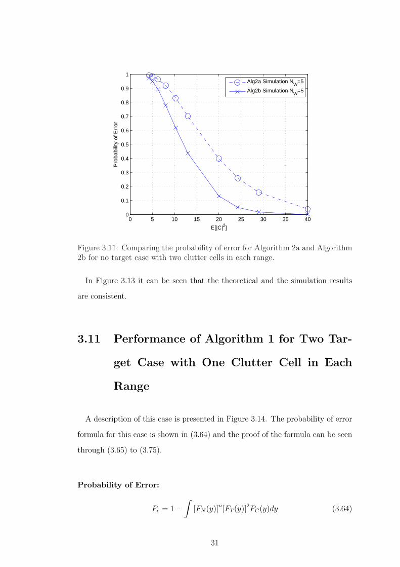
)(3.97)
= 2PC(y)− 2FC(y)PC(y) (3.98)
Pcor =
∫P (N < y)P (T < y)PC2
(y)dy (3.99)
=
∫[FN(y)]nFT (y) [2PC(y)− 2FC(y)PC(y)] dy (3.100)
Perr = 1− Pcor (3.101)
= 1−∫
[FN(y)]nFT (y) [2PC(y)− 2FC(y)PC(y)] dy (3.102)
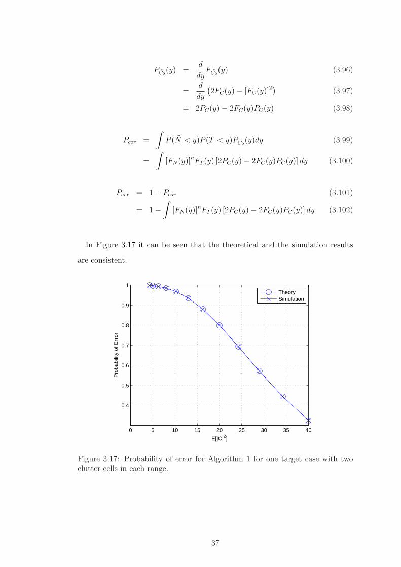
In Figure 3.17 it can be seen that the theoretical and the simulation results
are consistent.
0 5 10 15 20 25 30 35 40
0.4
0.5
0.6
0.7
0.8
0.9
1
E[|C|2]
Pro
babi
lity
of E
rror
TheorySimulation
Figure 3.17: Probability of error for Algorithm 1 for one target case with twoclutter cells in each range.
37
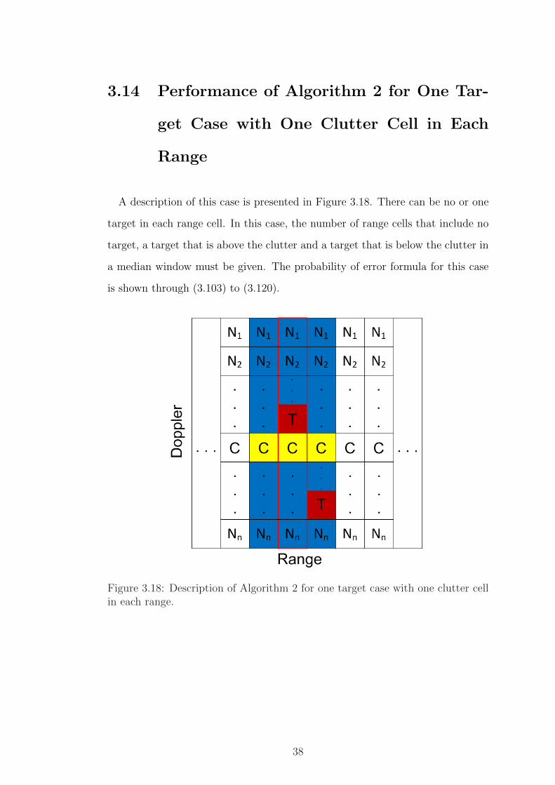
3.14 Performance of Algorithm 2 for One Tar-
get Case with One Clutter Cell in Each
Range
A description of this case is presented in Figure 3.18. There can be no or one
target in each range cell. In this case, the number of range cells that include no
target, a target that is above the clutter and a target that is below the clutter in
a median window must be given. The probability of error formula for this case
is shown through (3.103) to (3.120).
Figure 3.18: Description of Algorithm 2 for one target case with one clutter cellin each range.
38

Probability of Error:
Pe = (2K + 1)!
[2K+1∑
a=K+1
xa
a!
(2K+1−a∑
b=0
cby(2K+1−a−b)
b!(2K + 1− a− b)!
)]
+ (2K + 1)!
[2K+1∑
a=K+1
ya
a!
(2K+1−a∑
b=0
cbx(2K+1−a−b)
b!(2K + 1− a− b)!
)](3.103)
where c is the correct decision probability of position of clutter, x is the proba-
bility of deciding a cell that is above the clutter cell and y is the probability of
deciding a cell that is below the clutter cell in each range. Namely,
c =NTn
Nw
cTn +NTa
Nw
cTa +NTb
Nw
cTb(3.104)
x =NTn
Nw
xTn +NTa
Nw
xTa +NTb
Nw
xTb(3.105)
y =NTn
Nw
yTn +NTa
Nw
yTa +NTb
Nw
yTb(3.106)
where NTn is the number of range cells that include no target, NTa is the number
of range cells that include a target lying above clutter, NTbis the number of
range cells that include a target lying below the clutter and NW = 2K + 1 is
the median filter length. Here, cTn is the correct decision probability of clutter
when there is no target in a range cell, and cTa and cTbare the correct decision
probability of clutter when there is one target in a range cell. Actually, cTa is
equal to cTb. Up to now all the defined variables above are derived previously as
follows:
cTn =
∫(1− FC(z)) n [FN(z)]n−1PN(z)dz (3.107)
cTa = cTb=
∫[FN(y)]nFT (y)PC(y)dy (3.108)
In (3.105), xTn is the probability of deciding a bin that is above the clutter bin
when there is no target in a range cell, xTa is the probability of deciding a bin
that is above the clutter when a target lies above the clutter in a range cell, and
xTbis the probability of deciding a bin that is above the clutter when a target
lies below the clutter in a range cell. Similarly in (3.106), yTn is the probability
of deciding a bin that is below the clutter when there is no target in a range cell,
39

yTa is the probability of deciding a bin that is below the clutter when a target lies
above the clutter in a range cell, and yTbis the probability of deciding a bin that
is below the clutter when a target lies below the clutter in a range cell. Namely,
xTn = (1− c)ε (3.109)
yTn = (1− c)(1− ε) (3.110)
xTa = (1− c− t)ε + t (3.111)
yTa = (1− c− t)(1− ε) (3.112)
xTb= (1− c− t)ε (3.113)
yTb= (1− c− t)(1− ε) + t (3.114)
where ε is the ratio of the number of noise bins that is above the clutter bin
to the total number of noise bins in a range cell and t is the correct decision
probability of position of target, which is derived as follows:
t = P ((T > C)&(T > Ni, i = 1, ..., n)) (3.115)
= P ((T > C)&(T > max(N1, ..., Nn))) (3.116)
= P ((T > C)&(T > N)) (3.117)
=
∫P (C < t)P (N < t)PT (t)dt (3.118)
=
∫FC(t)FN(t)PT (t)dt (3.119)
=
∫FC(t)[FN(t)]nPT (t)dt (3.120)
In Figure 3.19 it can be observed that the theoretical and the simulation results
are consistent.
40
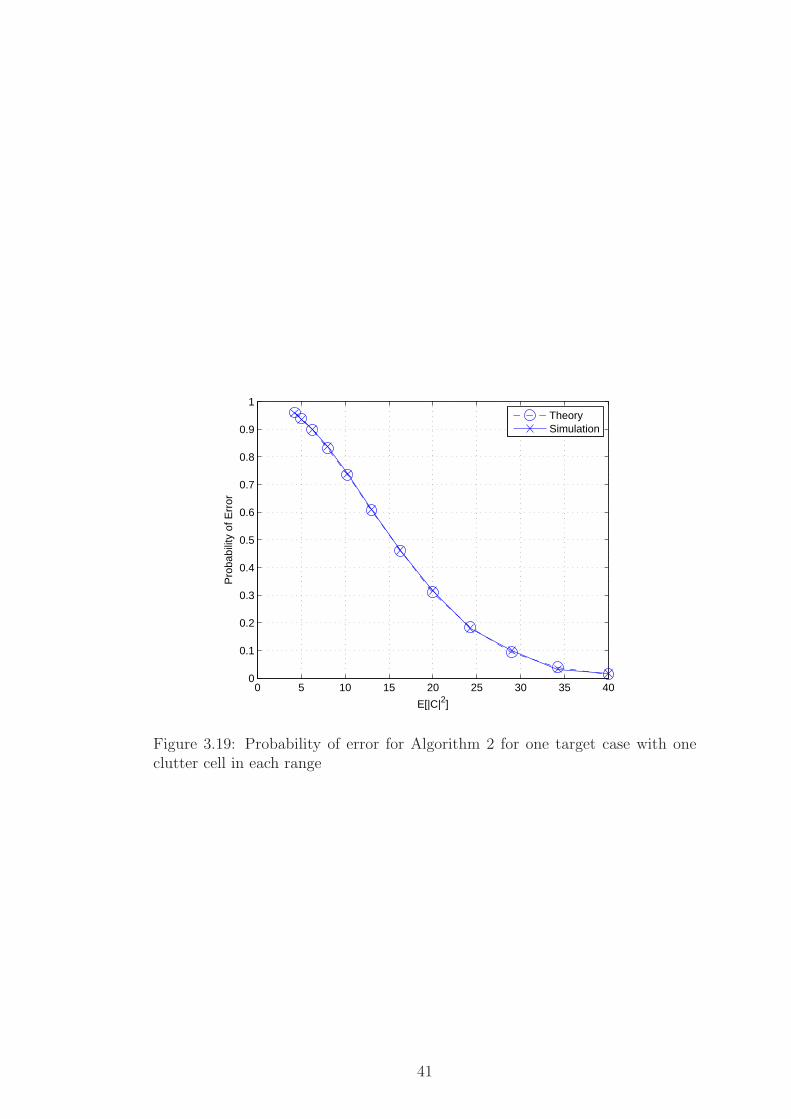
0 5 10 15 20 25 30 35 400
0.1
0.2
0.3
0.4
0.5
0.6
0.7
0.8
0.9
1
E[|C|2]
Pro
babi
lity
of E
rror
TheorySimulation
Figure 3.19: Probability of error for Algorithm 2 for one target case with oneclutter cell in each range
41

Chapter 4
SIMULATION RESULTS ON
REALISTIC DATA
In this chapter, the proposed clutter detection algorithms are run on some
realistic clutter data. Here, the clutter data is not taken from a real radar that
conducted an experiment on a real terrain. It is a synthetically generated data
based on a reasonable model of the real clutter data. For this reason, the word
“realistic” instead of “real” is used. The simulation results are compared with
the theoretical results to see whether they are consistent.
In order to get the realistic clutter data, first, a synthetic terrain is generated.
The terrain is generated in accordance with the reality [1]. It has vegetation
on smooth hills. Then, a synthetic radar is generated. This radar is modeled
as mounted on a helicopter platform. Therefore, the radar has a velocity. The
transmitted radar signal is reflected from the environment and then the radar
receives the reflected signal. After that, the signal is processed using pulse-
Doppler processing techniques. Finally, the realistic clutter data is obtained on
range-Doppler matrix for specific azimuth angles. The realistic data generating
system model was explained in detail in Chapter 2.
42
In some cases while performing simulations, targets are present in the environ-
ment. For such cases, synthetically generated point targets are used. In addition,
for some cases, a realistic target model is employed in the system. The realistic
target model used in the simulations are explained in Chapter 2.
In the simulations, a noise signal is added to the clutter and target signals.
Because the noise signal is synthetically generated, its parameter used in the
theoretical calculations are known. However, the clutter parameter is unknown.
In order to use the formulas derived in the previous chapter, the clutter parameter
should be estimated.
4.1 Clutter Statistics
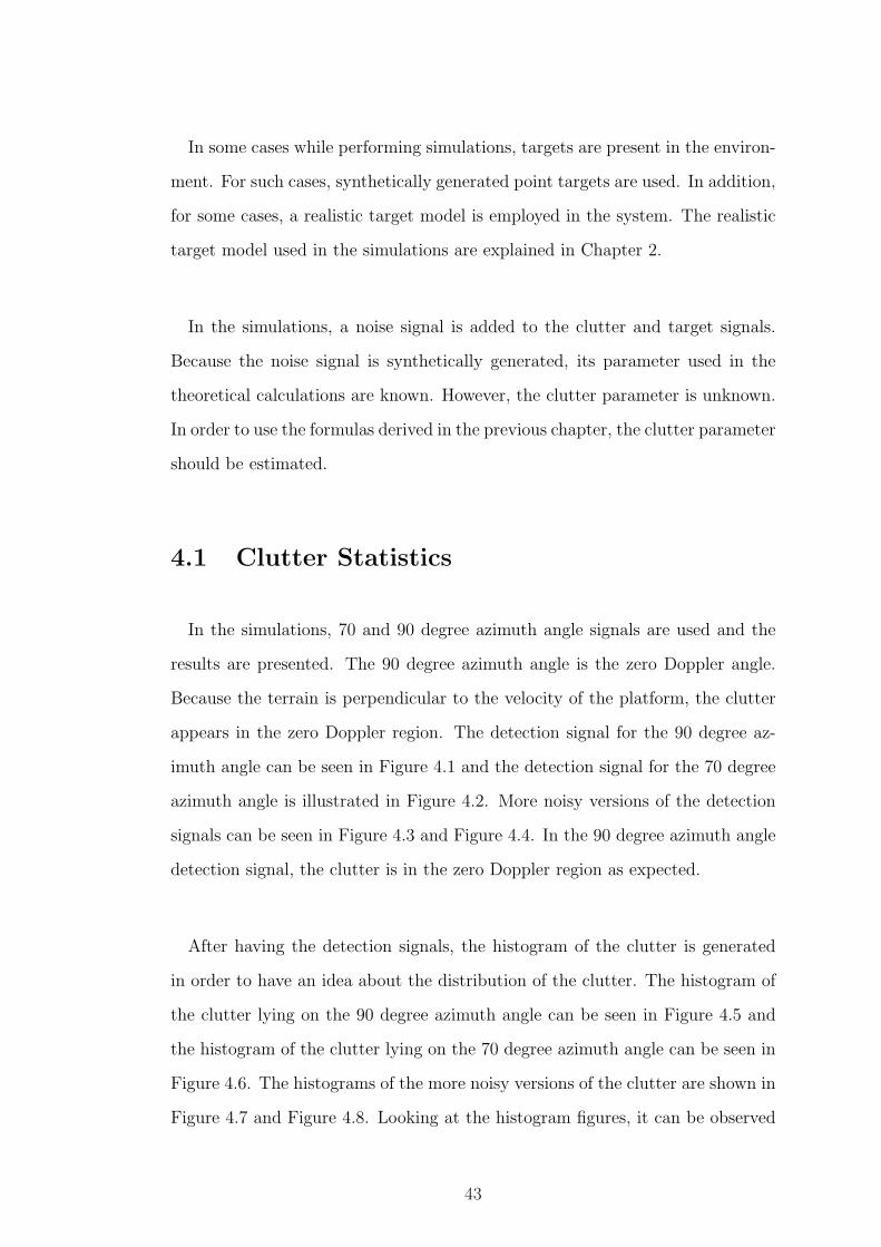
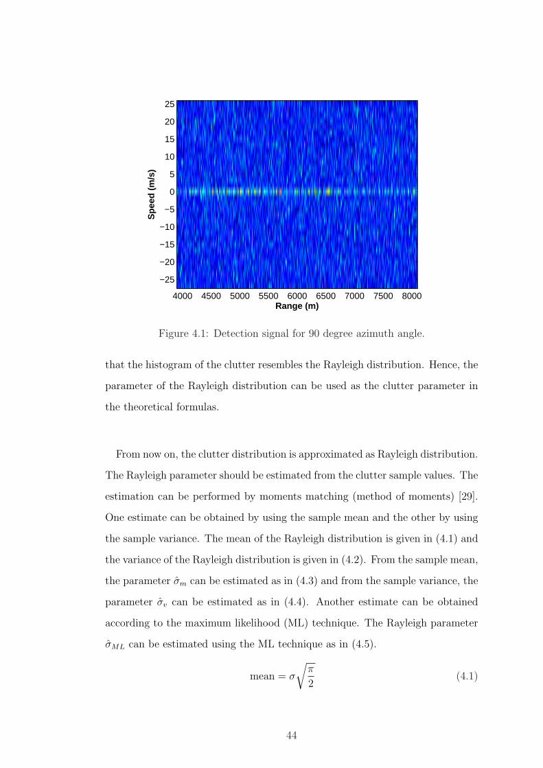
In the simulations, 70 and 90 degree azimuth angle signals are used and the
results are presented. The 90 degree azimuth angle is the zero Doppler angle.
Because the terrain is perpendicular to the velocity of the platform, the clutter
appears in the zero Doppler region. The detection signal for the 90 degree az-
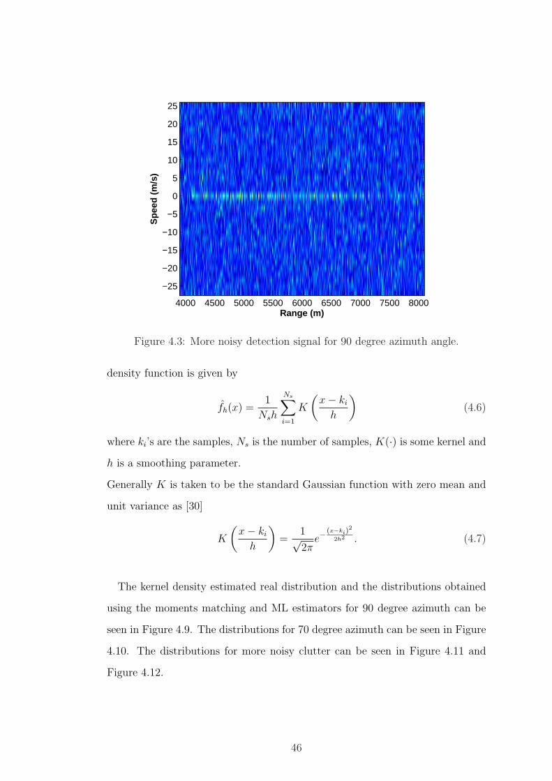
imuth angle can be seen in Figure 4.1 and the detection signal for the 70 degree
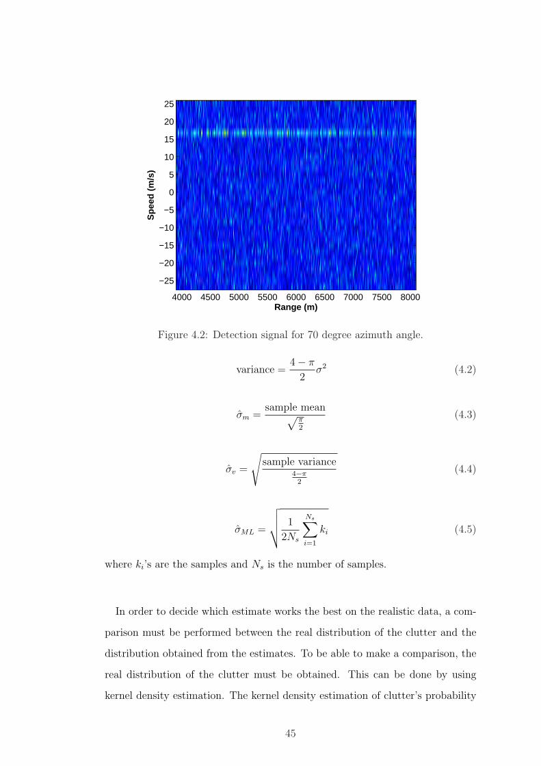
azimuth angle is illustrated in Figure 4.2. More noisy versions of the detection
signals can be seen in Figure 4.3 and Figure 4.4. In the 90 degree azimuth angle
detection signal, the clutter is in the zero Doppler region as expected.
After having the detection signals, the histogram of the clutter is generated
in order to have an idea about the distribution of the clutter. The histogram of
the clutter lying on the 90 degree azimuth angle can be seen in Figure 4.5 and
the histogram of the clutter lying on the 70 degree azimuth angle can be seen in
Figure 4.6. The histograms of the more noisy versions of the clutter are shown in
Figure 4.7 and Figure 4.8. Looking at the histogram figures, it can be observed
43
Range (m)
Sp
eed
(m
/s)
4000 4500 5000 5500 6000 6500 7000 7500 8000
−25
−20
−15
−10
−5
0
5
10
15
20
25
Figure 4.1: Detection signal for 90 degree azimuth angle.
that the histogram of the clutter resembles the Rayleigh distribution. Hence, the
parameter of the Rayleigh distribution can be used as the clutter parameter in
the theoretical formulas.
From now on, the clutter distribution is approximated as Rayleigh distribution.
The Rayleigh parameter should be estimated from the clutter sample values. The
estimation can be performed by moments matching (method of moments) [29].
One estimate can be obtained by using the sample mean and the other by using
the sample variance. The mean of the Rayleigh distribution is given in (4.1) and
the variance of the Rayleigh distribution is given in (4.2). From the sample mean,
the parameter σm can be estimated as in (4.3) and from the sample variance, the
parameter σv can be estimated as in (4.4). Another estimate can be obtained
according to the maximum likelihood (ML) technique. The Rayleigh parameter
σML can be estimated using the ML technique as in (4.5).
mean = σ
√π
2(4.1)
44
Range (m)
Sp
eed
(m
/s)
4000 4500 5000 5500 6000 6500 7000 7500 8000
−25
−20
−15
−10
−5
0
5
10
15
20
25
Figure 4.2: Detection signal for 70 degree azimuth angle.
variance =4− π
2σ2 (4.2)
σm =sample mean√
π2
(4.3)
σv =
√sample variance
4−π2
(4.4)
σML =
√√√√ 1
2Ns
Ns∑i=1
ki (4.5)
where ki’s are the samples and Ns is the number of samples.
In order to decide which estimate works the best on the realistic data, a com-
parison must be performed between the real distribution of the clutter and the
distribution obtained from the estimates. To be able to make a comparison, the
real distribution of the clutter must be obtained. This can be done by using
kernel density estimation. The kernel density estimation of clutter’s probability
45
Range (m)
Sp
eed
(m
/s)
4000 4500 5000 5500 6000 6500 7000 7500 8000
−25
−20
−15
−10
−5
0
5
10
15
20
25
Figure 4.3: More noisy detection signal for 90 degree azimuth angle.
density function is given by
fh(x) =1
Nsh
Ns∑i=1
K
(x− ki
h
)(4.6)
where ki’s are the samples, Ns is the number of samples, K(·) is some kernel and
h is a smoothing parameter.
Generally K is taken to be the standard Gaussian function with zero mean and
unit variance as [30]
K
(x− ki
h
)=
1√2π
e−(x−ki)
2
2h2 . (4.7)
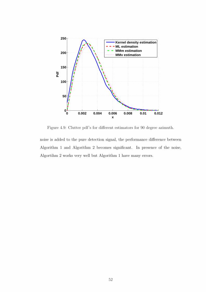
The kernel density estimated real distribution and the distributions obtained
using the moments matching and ML estimators for 90 degree azimuth can be
seen in Figure 4.9. The distributions for 70 degree azimuth can be seen in Figure
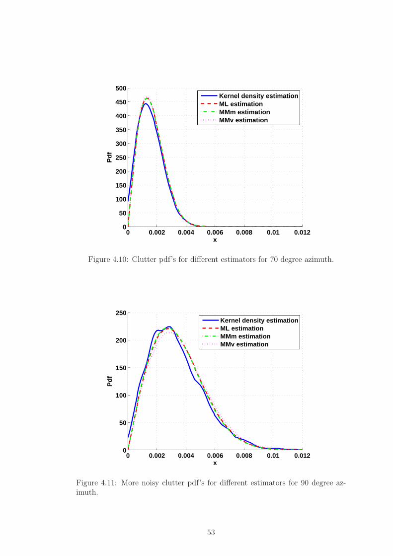
4.10. The distributions for more noisy clutter can be seen in Figure 4.11 and
Figure 4.12.
46
Range (m)
Sp
eed
(m
/s)
4000 4500 5000 5500 6000 6500 7000 7500 8000
−25
−20
−15
−10
−5
0
5
10
15
20
25
Figure 4.4: More noisy detection signal for 70 degree azimuth angle.
The comparison of the estimated density functions can be done using the
Kullback-Leibler divergence, which is a measure of the difference between two
probability distributions R and Q. Typically R represents a distribution which
is precisely calculated, and Q typically represents an approximation of R. The
KL distance is defined as [31]
DKL (R||Q) =
∞∫
−∞
r(x) logr(x)
q(x)dx. (4.8)
Here, R represents the clutter distribution calculated with kernel density estima-
tion and Q represents the moments matching and ML estimators of the clutter
distribution. The estimated parameters of the estimators and the results for the
KL distance can be seen in Table 4.1 and Table 4.2.
Looking at the KL distance results, it is observed that the minimum distance
to the clutter density is obtained with the density constructed using the ML
estimator in each and every trial. Among the estimators used, the ML estimator
has the best performance. From now on, in all the simulations using the realistic
47

0 0.002 0.004 0.006 0.008 0.01 0.012 0.0140
20
40
60
80
100
120
140
160
180
200
Amplitude
Num
ber
of a
mpl
itude
s
Figure 4.5: Histogram of clutter for 90 degree azimuth angle.
90 degree azimuth 70 degree azimuthσML 0.002615 0.002295σm 0.002591 0.002290σv 0.002702 0.002301
KLML 26.9430 1.33869KLm 28.0510 2.09471KLv 49.7358 29.1347
Table 4.1: Estimated parameters of clutter and KL distance results.
data, the distribution of the clutter used in the theoretical formulas will be
obtained using the ML estimator.
4.2 Simulation Results
In this section, the probability of error values are obtained for different clutter-
to-noise ratio (CNR) values. The simulation results are compared with the the-
oretical ones. The radar parameters and the platform on which the radar is
deployed allows a single clutter bin in each range cell, and the analysis is per-
formed accordingly.
48

0 1 2 3 4 5 6
x 10−3
0
20
40
60
80
100
120
140
160
180
Amplitude
Num
ber
of a
mpl
itude
s
Figure 4.6: Histogram of clutter for 70 degree azimuth angle.
90 degree azimuth 70 degree azimuthσML 0.002767 0.002284σm 0.002734 0.002282σv 0.002887 0.002293
KLML 6.23070 25.5667KLm 8.496880 26.6492KLv 42.8982 30.2588
Table 4.2: Estimated parameters of more noisy clutter and KL distance results.
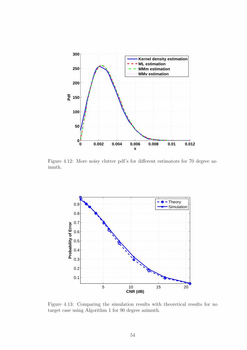
The comparison of the theoretical and simulation results with no target using
Algorithm 1 for 90 degree azimuth is presented in Figure 4.13 and for 70 degree
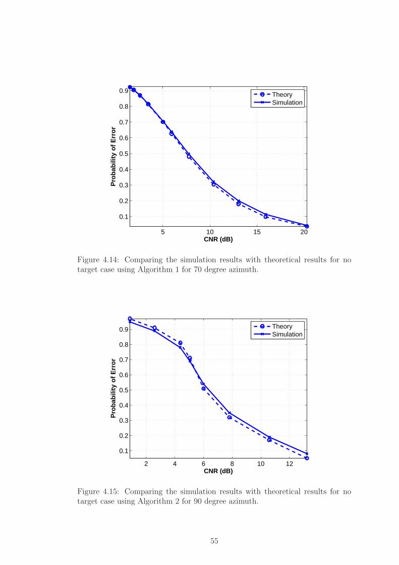
azimuth is shown in Figure 4.14.
The comparison of the theoretical and simulation results with no target using
Algorithm 2 for 90 degree azimuth is presented in Figure 4.15 and for 70 degree
azimuth is given in Figure 4.16.
49

0 0.002 0.004 0.006 0.008 0.01 0.0120
20
40
60
80
100
120
140
160
180
Amplitude
Num
ber
of a
mpl
itude
s
Figure 4.7: Histogram of more noisy clutter for 90 degree azimuth angle.
The comparison of the theoretical and simulation results with one point target
using Algorithm 1 for 90 degree azimuth is given in Figure 4.17 and for 70 degree
azimuth is shown in Figure 4.18.
From Figure 4.13 to Figure 4.18, the figures for 90 degree azimuth and the
ones for 70 degree azimuth are similar in each case. Also, the theoretical and the
simulation results are not matched perfectly but it is observed that the results
are very close. This situation has reasonable causes. One of the reasons is that
the estimated clutter distribution is used instead of the real distribution of the
clutter. From Figure 4.9 to Figure 4.12, it can be seen that the kernel density
estimated distribution does not perfectly match the distribution obtained from
the ML estimator. The other reason is that it is assumed that the clutter is
present in only one cell for each range cell. Actually, the clutter mainly stays in
one cell but a weak spread occurs along the range cell. Those reasons are behind
the situation of the slight mismatch between the theory and the simulation.
50
0 0.002 0.004 0.006 0.008 0.01 0.0120
20
40
60
80
100
120
140
160
Amplitude
Num
ber
of a
mpl
itude
s
Figure 4.8: Histogram of more noisy clutter for 70 degree azimuth angle.
Comparing Figure 4.13 and Figure 4.15, it can be observed that Algorithm 2
has better performance than Algorithm 1, as expected. Algorithm 2 achieves a
0.05 probability of error with a 13 dB CNR while Algorithm 1 achieves the same
probability of error with a 20 dB CNR.
Up to now, the comparison between the theoretical results and the simulation
results are performed. The following discussion will be on the results of the
algorithms on the range-Doppler matrix. In Figure 4.19, the noiseless detection
signal with a realistic target for 90 degree azimuth can be seen. In Figure 4.20,
the result of Algorithm 1 are shown and in Figure 4.21 the result of Algorithm 2
are illustrated. When noise is added to the noiseless detection signal, the results
of Algorithm 1 and Algortihm 2 can be seen in Figure 4.22 and Figure 4.23,
respectively.
As seen from the figures, both algorithms work well in the absence of noise.
However, Algorithm 1 have errors when a target is present as expected. When
51
0 0.002 0.004 0.006 0.008 0.01 0.0120
50
100
150
200
250
x
Pd
f
Kernel density estimationML estimationMMm estimationMMv estimation
Figure 4.9: Clutter pdf’s for different estimators for 90 degree azimuth.
noise is added to the pure detection signal, the performance difference between
Algorithm 1 and Algorithm 2 becomes significant. In presence of the noise,
Algortihm 2 works very well but Algorithm 1 have many errors.
52
0 0.002 0.004 0.006 0.008 0.01 0.0120
50
100
150
200
250
300
350
400
450
500
x
Pd
f
Kernel density estimationML estimationMMm estimationMMv estimation
Figure 4.10: Clutter pdf’s for different estimators for 70 degree azimuth.
0 0.002 0.004 0.006 0.008 0.01 0.0120
50
100
150
200
250
x
Pd
f
Kernel density estimationML estimationMMm estimationMMv estimation
Figure 4.11: More noisy clutter pdf’s for different estimators for 90 degree az-imuth.
53
0 0.002 0.004 0.006 0.008 0.01 0.0120
50
100
150
200
250
300
x
Pd
f
Kernel density estimationML estimationMMm estimationMMv estimation
Figure 4.12: More noisy clutter pdf’s for different estimators for 70 degree az-imuth.
5 10 15 20
0.1
0.2
0.3
0.4
0.5
0.6
0.7
0.8
0.9
CNR (dB)
Pro
bab
ility
of
Err
or
TheorySimulation
Figure 4.13: Comparing the simulation results with theoretical results for notarget case using Algorithm 1 for 90 degree azimuth.
54
5 10 15 20
0.1
0.2
0.3
0.4
0.5
0.6
0.7
0.8
0.9
CNR (dB)
Pro
bab
ility
of
Err
or
TheorySimulation
Figure 4.14: Comparing the simulation results with theoretical results for notarget case using Algorithm 1 for 70 degree azimuth.
2 4 6 8 10 12
0.1
0.2
0.3
0.4
0.5
0.6
0.7
0.8
0.9
CNR (dB)
Pro
bab
ility
of
Err
or
TheorySimulation
Figure 4.15: Comparing the simulation results with theoretical results for notarget case using Algorithm 2 for 90 degree azimuth.
55
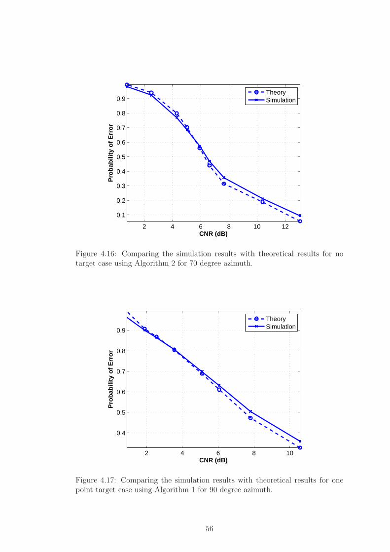
2 4 6 8 10 12
0.1
0.2
0.3
0.4
0.5
0.6
0.7
0.8
0.9
CNR (dB)
Pro
bab
ility
of
Err
or
TheorySimulation
Figure 4.16: Comparing the simulation results with theoretical results for notarget case using Algorithm 2 for 70 degree azimuth.
2 4 6 8 10
0.4
0.5
0.6
0.7
0.8
0.9
CNR (dB)
Pro
bab
ility
of
Err
or
TheorySimulation
Figure 4.17: Comparing the simulation results with theoretical results for onepoint target case using Algorithm 1 for 90 degree azimuth.
56
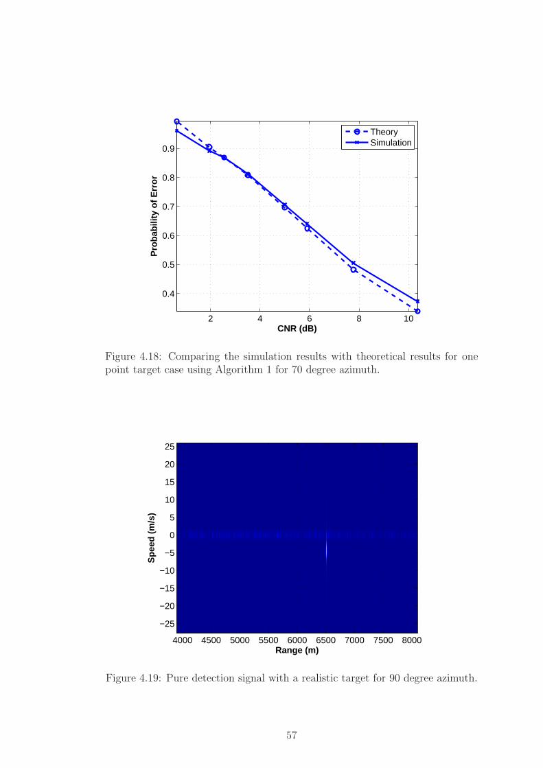
2 4 6 8 10
0.4
0.5
0.6
0.7
0.8
0.9
CNR (dB)
Pro
bab
ility
of
Err
or
TheorySimulation
Figure 4.18: Comparing the simulation results with theoretical results for onepoint target case using Algorithm 1 for 70 degree azimuth.
Range (m)
Sp
eed
(m
/s)
4000 4500 5000 5500 6000 6500 7000 7500 8000
−25
−20
−15
−10
−5
0
5
10
15
20
25
Figure 4.19: Pure detection signal with a realistic target for 90 degree azimuth.
57
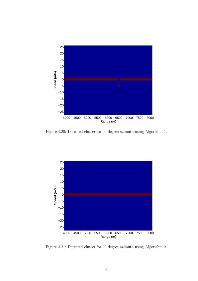
Range (m)
Sp
eed
(m
/s)
4000 4500 5000 5500 6000 6500 7000 7500 8000
−25
−20
−15
−10
−5
0
5
10
15
20
25
Figure 4.20: Detected clutter for 90 degree azimuth using Algorithm 1.
Range (m)
Sp
eed
(m
/s)
4000 4500 5000 5500 6000 6500 7000 7500 8000
−25
−20
−15
−10
−5
0
5
10
15
20
25
Figure 4.21: Detected clutter for 90 degree azimuth using Algorithm 2.
58
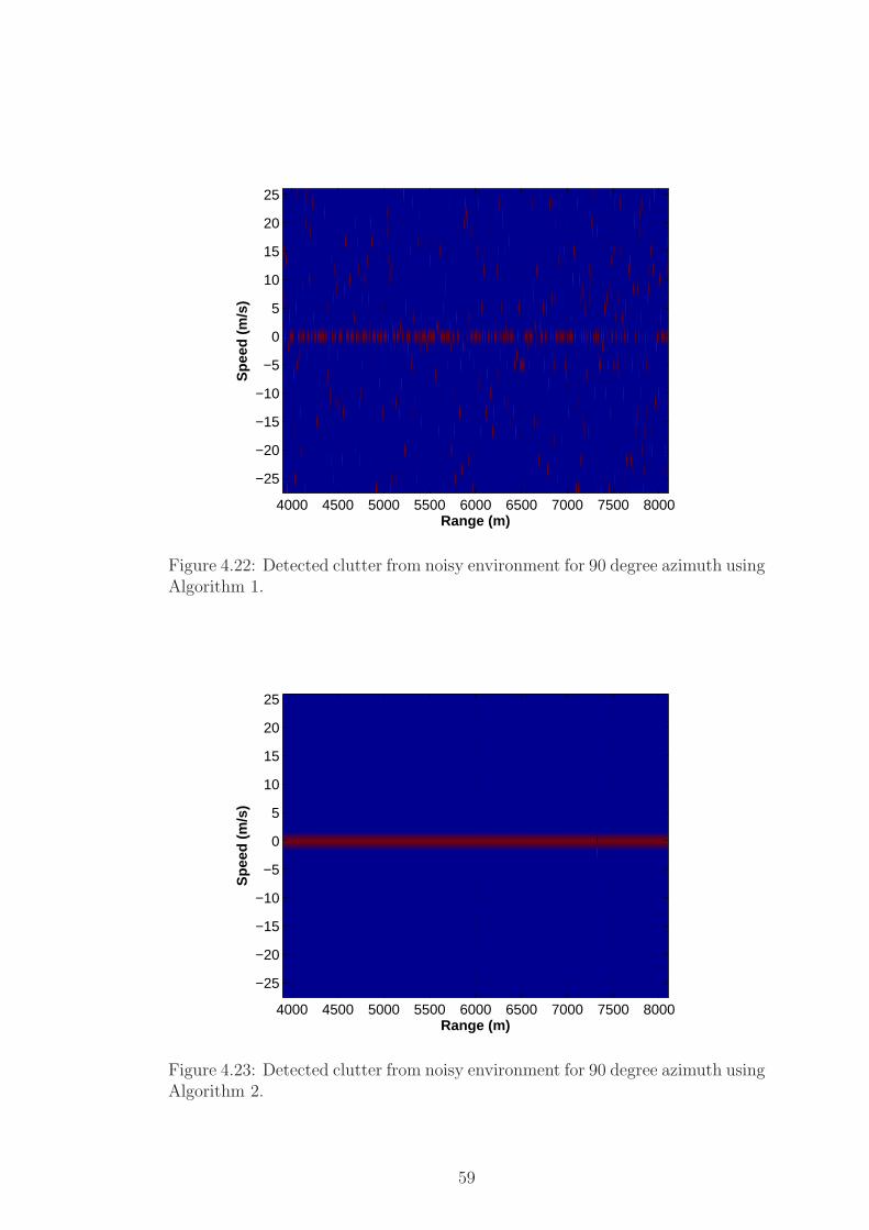
Range (m)
Sp
eed
(m
/s)
4000 4500 5000 5500 6000 6500 7000 7500 8000
−25
−20
−15
−10
−5
0
5
10
15
20
25
Figure 4.22: Detected clutter from noisy environment for 90 degree azimuth usingAlgorithm 1.
Range (m)
Sp
eed
(m
/s)
4000 4500 5000 5500 6000 6500 7000 7500 8000
−25
−20
−15
−10
−5
0
5
10
15
20
25
Figure 4.23: Detected clutter from noisy environment for 90 degree azimuth usingAlgorithm 2.
59

Chapter 5
CONCLUSIONS AND FUTURE
WORK
In this thesis, various algorithms have been investigated for clutter detection in
pulse-Doppler radar systems. The main idea behind the algorithms is that since
the clutter generally has higher amplitude compared to noise values in a range-
Doppler matrix, it can be used to perform precise detection of clutter. Since
clutter detection is a real-time military process, it is vital to detect the clutter
independent of other parameters as quick as possible with strictly defined algo-
rithms unlike the algorithms proposed in literature. The first algorithm has low
computational complexity. This aspect of the algorithm allows quick detection.
Algorithm 1 selects the maximum valued cell as the clutter cell in each range
in the range-Doppler matrix. When only clutter and noise are present, this al-
gorithm works well. However, if a target is added to the range-Doppler matrix,
the algorithm may cause erronous results because targets generally have higher
amplitudes than clutter in the range-Doppler matrix. At this point, Algorithm 2
supplies a correction. The outputs of Algorithm 1 is median filtered and improved
results can be obtained. However, this correction increases the computational
60
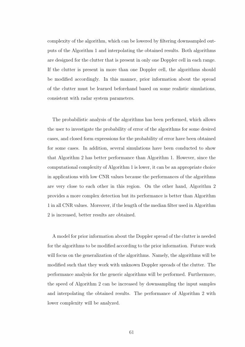
complexity of the algorithm, which can be lowered by filtering downsampled out-
puts of the Algorithm 1 and interpolating the obtained results. Both algorithms
are designed for the clutter that is present in only one Doppler cell in each range.
If the clutter is present in more than one Doppler cell, the algorithms should
be modified accordingly. In this manner, prior information about the spread
of the clutter must be learned beforehand based on some realistic simulations,
consistent with radar system parameters.
The probabilistic analysis of the algorithms has been performed, which allows
the user to investigate the probability of error of the algorithms for some desired
cases, and closed form expressions for the probability of error have been obtained
for some cases. In addition, several simulations have been conducted to show
that Algorithm 2 has better performance than Algorithm 1. However, since the
computational complexity of Algorithm 1 is lower, it can be an appropriate choice
in applications with low CNR values because the performances of the algorithms
are very close to each other in this region. On the other hand, Algorithm 2
provides a more complex detection but its performance is better than Algorithm
1 in all CNR values. Moreover, if the length of the median filter used in Algorithm
2 is increased, better results are obtained.
A model for prior information about the Doppler spread of the clutter is needed
for the algorithms to be modified according to the prior information. Future work
will focus on the generalization of the algorithms. Namely, the algorithms will be
modified such that they work with unknown Doppler spreads of the clutter. The
performance analysis for the generic algorithms will be performed. Furthermore,
the speed of Algorithm 2 can be increased by downsampling the input samples
and interpolating the obtained results. The performance of Algorithm 2 with
lower complexity will be analyzed.
61
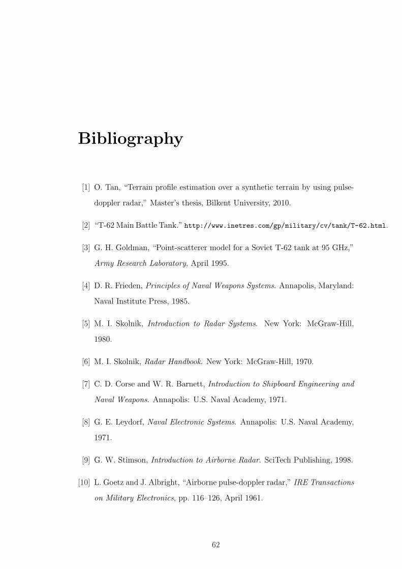
Bibliography
[1] O. Tan, “Terrain profile estimation over a synthetic terrain by using pulse-
doppler radar,” Master’s thesis, Bilkent University, 2010.
[2] “T-62 Main Battle Tank.” http://www.inetres.com/gp/military/cv/tank/T-62.html.
[3] G. H. Goldman, “Point-scatterer model for a Soviet T-62 tank at 95 GHz,”
Army Research Laboratory, April 1995.
[4] D. R. Frieden, Principles of Naval Weapons Systems. Annapolis, Maryland:
Naval Institute Press, 1985.
[5] M. I. Skolnik, Introduction to Radar Systems. New York: McGraw-Hill,
1980.
[6] M. I. Skolnik, Radar Handbook. New York: McGraw-Hill, 1970.
[7] C. D. Corse and W. R. Barnett, Introduction to Shipboard Engineering and
Naval Weapons. Annapolis: U.S. Naval Academy, 1971.
[8] G. E. Leydorf, Naval Electronic Systems. Annapolis: U.S. Naval Academy,
1971.
[9] G. W. Stimson, Introduction to Airborne Radar. SciTech Publishing, 1998.
[10] L. Goetz and J. Albright, “Airborne pulse-doppler radar,” IRE Transactions
on Military Electronics, pp. 116–126, April 1961.
62

[11] U. DiNardo and G. Nucci, “Synthesis criteria of a signal processor for pulse
doppler radars,” Selenia Technical Review, September 1972.
[12] R. O’Donnel et al., “Advanced signal processing for airport surveillance
radars,” IEEE Eascon Record, pp. 71–71F, 1974.
[13] R. Daly and J. Glass, “Digital signal processing for radar,” Electronic
Progress, pp. 24–30, Spring 1975.
[14] R. Mooney and G. Ralston, “Performance in clutter of airborne pulse mti,
cw doppler and pulse doppler radar,” IRE Convention Record, pp. 55–62,
1961.
[15] E. Pearson et al., Method of Tracking Target in Presence of Clutter. US
Patent 4559537, 1985.
[16] S. Clancy et al., Method and System for Tracking Targets in a Pulse Doppler
Radar System. US Patent 4450446, 1984.
[17] F. Tony and A. Luminita, “Active contours without edges,” IEEE Transac-
tions On Image Processing, pp. 266–277, February 2001.
[18] E. Ma, “Simulating nature,” Project A, June 2002.
[19] G. Macklem, “Computer landscape generation and smoothing,” Masters
Comprehensive Exam, 2003.
[20] H. Sogancı, “Doppler frequency estimation in pulse doppler radar systems,”
Master’s thesis, Bilkent University, 2009.
[21] M. A. Richards, Fundamentals of Radar Signal Processing. New York:
McGraw-Hill, 2005.
[22] C. E. Cook and M. Bernfeld, Radar Signals An Introduction to Theory and
Application. London: Artech House, 1993.
[23] N. Levanon and E. Mozeson, Radar Signals. New York: Wiley, 2004.
63
[24] T. W. Jeffrey, Phased-Array Radar Design. Raleigh, NC: SciTech Publish-
ing, 2009.
[25] D. K. Barton, Radar System Analysis and Modeling. Norwood, MA: Artech
House, 2005.
[26] G. Morris and L. Harkness, Airborne Pulsed Doppler Radar. Boston: Artech
House.
[27] N. Levanon, Radar Principles. New York: Wiley, 1988.
[28] P. Z. Peebles, Radar Principles. New York: Wiley, 1998.
[29] M. Bulmer, Principles of Statistics. Dover, 1979.
[30] M. Jones and J. Marron, “A brief survey of bandwidth selection for density
estimation,” Journal of the American Statistical Association, pp. 401–407,
Mar. 1996.
[31] S. Kullback and R. Leibler, “On information and sufficiency,” Annals of
Mathematical Statistics, pp. 79–86, 1951.
64