Clustering Microarray Data

Andrea Vijverberg

Advisor: Professor Hardin

Pomona College

Department of Mathematics

Spring 2007

Contents

1 Introduction 1

2 Background 32.1 Microarrays . . . . . . . . . . . . . . . . . . . . . . . . . . . . . . 3

3 Cluster Analysis 53.1 Distance Metrics . . . . . . . . . . . . . . . . . . . . . . . . . . . 53.2 Clustering Techniques . . . . . . . . . . . . . . . . . . . . . . . . 73.3 Evaluation Methods . . . . . . . . . . . . . . . . . . . . . . . . . 12

3.3.1 Maximizing Average Silhouette Width . . . . . . . . . . . 123.3.2 Minimizing Mean Split Silhouette . . . . . . . . . . . . . 133.3.3 L Method . . . . . . . . . . . . . . . . . . . . . . . . . . . 133.3.4 Bootstrap Method . . . . . . . . . . . . . . . . . . . . . . 14

4 Data 16

5 Results and Discussion 185.1 Clustering . . . . . . . . . . . . . . . . . . . . . . . . . . . . . . . 185.2 Evaluation Methods . . . . . . . . . . . . . . . . . . . . . . . . . 19

5.2.1 Optimal Number of Clusters . . . . . . . . . . . . . . . . 195.2.2 Bootstrap . . . . . . . . . . . . . . . . . . . . . . . . . . . 20

5.3 Further Results . . . . . . . . . . . . . . . . . . . . . . . . . . . . 20

6 Conclusion 22References . . . . . . . . . . . . . . . . . . . . . . . . . . . . . . . . . . 22

1

List of Tables

6.1 HOPACH clustering on Pearson’s correlation sample using Pear-son’s correlation distance metric . . . . . . . . . . . . . . . . . . 25

6.2 Comparison of Original and “Improved” Samples using Pearson’sCorrelation . . . . . . . . . . . . . . . . . . . . . . . . . . . . . . 25

6.3 Comparison of Original and “Improved” Samples using Percent-age Bend Correlation . . . . . . . . . . . . . . . . . . . . . . . . . 25

2

List of Figures

6.1 A Microarray Chip . . . . . . . . . . . . . . . . . . . . . . . . . . 266.2 Hierarchical Clustering Dendrogram of Pearson’s Correlation Sam-

ple using Pearson’s Correlation Distance Metric . . . . . . . . . . 266.3 Hierarchical Clustering Dendrogram of Pearson’s Correlation Sam-

ple using Percentage Bend Correlation Distance Metric . . . . . . 276.4 PAM Partitioning of Percentage Bend Correlation Sample using

Percentage Bend Correlation Distance Metric . . . . . . . . . . . 276.5 PAM Partitioning of Percentage Bend Correlation Sample using

Pearson’s Correlation Distance Metric . . . . . . . . . . . . . . . 286.6 HOPACH Heat Map of Pearson’s Correlation Sample using Pear-

son’s Correlation Distance Metric . . . . . . . . . . . . . . . . . . 286.7 Average Silhouette of Percentage Bend Correlation Sample using

Percentage Bend Correlation Distance Metric . . . . . . . . . . . 296.8 Average Silhouette of Pearson’s Correlation Sample using Pear-

son’s Correlation Distance Metric . . . . . . . . . . . . . . . . . . 296.9 Mean Split Silhouette of Percentage Bend Correlation Sample

using Pearson’s Correlation Distance Metric . . . . . . . . . . . . 306.10 L Method on PAM Results of Percentage Bend Correlation Sam-

ple using Percentage Bend Correlation Distance Metric . . . . . . 306.11 L Method on PAM Results of Pearson’s Correlation Sample using

Percentage Bend Correlation Distance Metric . . . . . . . . . . . 316.12 L Method on PAM Results of Percentage Bend Correlation Sam-

ple using Euclidean Distance Metric . . . . . . . . . . . . . . . . 316.13 Original Sample Bootstrap Plot . . . . . . . . . . . . . . . . . . . 326.14 Improved Sample Bootstrap Plot . . . . . . . . . . . . . . . . . . 336.15 Boxplot of Proportions of Genes in the Correct Cluster . . . . . . 34

3

Abstract

Using microarray data, which gives thousands of genes’ expression levels at once,we examine different clustering techniques and evaluation methods to effectivelycluster the noisy data. The results of this study has implications for the field ofbiology. Genes with similar functions are grouped together, which gives insightinto specific genes and their role in the cell. The cluster analysis employeduses different distance metrics, including Euclidean, Pearson’s correlation, andpercentage bend correlation, and we use the cluster methods of hierarchical,Partitioning Around Medoids (PAM), and Hierarchical Ordered Partitioningand Collapsing Hybrid (HOPACH). The evaluation methods involve silhouettewidth, the L method, and the bootstrap. We conclude with an experiment inimproving the sample and the clustering output using the bootstrap method.

Chapter 1

Introduction

In order to measure genetic activity, scientists aim to discover the bio-logical functions of specific genes. By clustering the expressed genes, which playan important role in the function of the cells, biologists can further understandspecific genes and their role in the cell. The statistician clusters the genes byfirst using a measure of dissimilarity between the genes and then clustering thegenes using a clustering algorithm. Afterwards, we test the clustering results todetermine their stability.

In this project, we will use microarray data, which gives thousands ofgenes’ levels of expression at once. Microarray data is very noisy, requiring arobust measure of dissimilarity. Different distance metrics will be briefly com-pared in their robustness. Several clustering methods will be employed, includ-ing hierarchical, partitioning, and a hybrid of the two. To estimate the strengthof cluster membership, we apply the bootstrap. Bootstrap methods may be ap-plied in several different ways, but the general method is as follows: create manyresamples by sampling with replacement from the original sample and find thebootstrap distribution of the statistic from the resamples. In our case of clus-tering microarray data, we have one data set, and, by creating and clusteringmany resamples, we can determine the reproducibility of the clustering resultand which genes cluster poorly. Instead of finding a bootstrap distribution, asin the general theory, we examine the variability of the cluster output.

The following section will give a more detailed description of microarraysand how the data are obtained. Chapter 3 will look at cluster analysis. Themain mathematical background information, such as distance metrics and clus-tering theory, comes from Draghici [1], Johnson and Wichern [3], Kaufman andRousseeuw [4], and Wilcox [10]. The specific clustering algorithms, PartitioningAround Medoids (PAM) and Hierarchical Ordered Partitioning and CollapsingHybrid (HOPACH), were developed by Kaufman and Rousseeuw [4] and Vander Laan and Pollard [8], respectively. The description of the algorithms are fol-lowed by the theory on evaluation methods, drawing from the works of Salvadorand Chan [7] for the L method and Van der Laan and Pollard [8] and [9] for thebootstrap criterion. Using Mooney and Duval [5] and Efron and Tibshirani [2],

1

I explain the theory on bootstrap techniques.Chapter 4 will explain the data and Chapter 5 will use the clustering

algorithms and tests on the data, giving graphs and a discussion of the results.Finally, I will conclude with a recap of the major results and possible furtherextensions on this project.

2

Chapter 2

Background

2.1 Microarrays

A microarray is a small chip that has thousands of single strands ofgenetic material tethered to it. Its creation begins with a process of denaturinga cell’s mRNA into single strands and then attaching them to the chip. Eachgene in the cell is represented by a dot on the chip, but not all possible genes arenecessary for a particular cell to perform its function. For example, a blood cellonly uses genes that aid in the functions of a blood cell which might be differentfrom those a skin cell would use. We call the functional genes of the cell theexpressed genes. Therefore, when a cell becomes diseased, say with cancer,certain expressed genes may have changed, causing the misbehavior of the cell.A microarray chip allows researchers to examine, all at once, the expressed genesof a cell in both healthy and unhealthy samples.

To analyze these gene functions, biologists take samples from cells knownto be healthy or diseased and allow their single strands of DNA to attach tothose on the microarray chip. This is done by gathering the mRNA of theseknown cells, which comes out of the cell nucleus during cell replication andgives the genetic code of the expressed genes. Using the mRNA to make cDNAand labelling the cDNA with a color of red or green, the expressed genes onthe chip become labelled with the colors of the attaching cDNA, as the doublehelix reforms. The assignment of colors to the cDNA depends on its respectivesample, experiment or control. Note that not all of the genes on the chip re-formthe double helix with the cDNA because, as mentioned before, not all the geneson the chip are used in a cell’s function.

The chip is scanned twice under a fluorescent light, once measuring thegreen color intensities and once measuring the red. Putting these scans together,each spot on the chip appears in one of four colors (Figure 6.1). A black spotmeans the gene is not expressed, i.e., no labelled cDNA attached to any genesin that spot. A yellow dot has genes of both samples expressed equally. A greenspot has more of the green sample expressed, and similarly, the red spot has

3

more expression from the red sample.Scanning the chip quantifies the fluorescence of each dot: more fluores-

cence means more of the sample stuck to the chip. Due to the double scan, eachspot on the chip has a numerical value for red and green color intensity. Puttingthese numbers together, we obtain our data set which is of the log ratios of colorintensities for each spot.

4

Chapter 3

Cluster Analysis

With the goal of assisting scientists in measuring genetic activity, manygenes at a time, we would like to cluster the genes. Scientists can use the cluster-ing results to learn how genes are co-regulated, giving them insight into certaingenes’ relation to each other and their functions. Since we do not have priorknowledge of which genes are related, we take on the “unsupervised learning”strategy of clustering, which is the ideal approach in cases where one has nopreconceived knowledge of the groupings. Clustering is the process of groupingtogether similar entities. Any data set can be clustered, so the final goal is notthe clustering result itself but the conclusions that can be drawn. With this inmind, we will apply different clustering techniques and compare the results.

Before we begin discussing clustering techniques, we must select a mea-sure of similarity or dissimilarity between the genes. As one of our goals, wewould like to compare robust distances with others to see which provides betterclustering results. In particular, we will be using two non-robust distances, Eu-clidean distance and Pearson’s correlation, and the robust distance of percentagebend correlation.

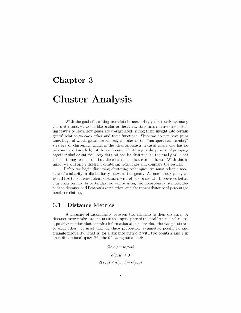
3.1 Distance Metrics

A measure of dissimilarity between two elements is their distance. Adistance metric takes two points in the input space of the problem and calculatesa positive number that contains information about how close the two points areto each other. It must take on three properties: symmetry, positivity, andtriangle inequality. That is, for a distance metric d with two points x and y inan n-dimensional space �n, the following must hold:

d(x, y) = d(y, x)

d(x, y) ≥ 0

d(x, y) ≤ d(x, z) + d(z, y)

5

where z is a third point.Typically, researchers use the Euclidean distance, whose numerical value

stems from the Pythagorean Theorem. This distance, used for most practicalpurposes, is defined as

dE(x, y) =√

(x1 − y1)2 + (x2 − y2)2 + ... + (xn − yn)2 =

√√√√n∑

i=1

(xi − yi)2

The other most common distance metric used is the Pearson’s correlation dis-tance:

dR(x, y) = 1 − rxy

where rxy is the Pearson’s correlation coefficient of the vectors x and y:

rxy =Sxy√

Sx

√Sy

=

n∑i=1

(xi − x)(yi − y)

√√√√n∑

i=1

(xi − x)2

√√√√n∑

i=1

(yi − y)2

where x and y are the sample means.Since the Pearson’s correlation coefficient rxy varies only between -1 and

1, the distance will take values between 0 and 2. When a pair of elements arepositively perfectly correlated, the correlation will be 1 and the distance willbe zero. Similarly, a negatively perfectly correlated pair will have a distance of2. Intuitively, smaller distances are assigned to pairs that change similarly. Forexample, the distance between an element and itself is zero since it is perfectlycorrelated with itself.

In general, the Pearson’s correlation distance metric evaluates how genesmove in relation to each other, whereas the Euclidean distance calculates theactual numerical difference in space between the vectors. Suppose there arethree genes A, B, and C. In relation to gene A, gene B changes more similarlythan gene C does but gene C is closer to gene A. Using Pearson’s correlationdistance metric, the distance between genes A and B is smaller than the distancebetween genes A and C. However, the Euclidean distance metric will give asmaller distance value for the pair A and C than for the pair A and B. Thesimple example shows the potential for a discrepancy in the final result thatstems from the choice in distance metrics.

Another issue arises concerning the robustness of the Pearson’s correla-tion distance metric. Well known in the statistical literature, Pearson’s correla-tion lacks robustness because one point in one of the marginal distributions canhave a large effect on rxy. Therefore, we use a more robust distance metric, thepercentage bend correlation. Given one point (x, y), we calculate the samplemedian Mx and My, which we use to calculate Wi, Wi =| xi − Mx |. We rankthe Wi values in ascending order: W(1) ≤ W(2) ≤ ... ≤ W(n). Set ωx = W(m).

6

Let i1 be the number of xi values for which xi−Mx

ωx< −1 and let i2 be the num-

ber of xi values such that xi−Mx

ωx> 1. Let Sx =

n−i2∑i=i1+1

x(i). Similar calculations

are done for the y variable. The percentage bend correlation is given by thefollowing equation (Wilcox [10]):

rpb =∑

AiBi√∑A2

i

∑B2

i

where Ai = Ψ(Ui) and Bi = Ψ(Vi), Ψ(x) = max[−1, min(1, x)], Ui = (xi −φx)/ωx and Vi = (yi − φy)/ωy and φx = ωx(i2−i1)+Sx

n−i1−i2. The variables Ui and

Vi represent a scaled distance from the center. Hence, the extreme outliers areset to a specific limit, so that they do not impact the correlation value as heav-ily. This adjustment makes the percentage bend correlation more robust thanPearson’s correlation. For both the Pearson’s correlation and the percentagebend correlation, the triangle inequality does not hold, but when discussingsimilarities, we often drop this requirement.

3.2 Clustering Techniques

Using the above distance metrics, we create a measure of similarity be-tween genes, which is one minus the distance. Clustering results depend highlyon the distance metric used. After calculating a distance matrix giving the dis-tances of every element with respect to all the others, we employ a clusteringtechnique. In this project, we focus on three methods: hierarchical clustering,partitioning around medoids (PAM), and hierarchical ordered partitioning andcollapsing hybrid (HOPACH).

In clustering microarray data, hierarchical clustering has typically beenused because the covariance structure of the data is not needed. The final resultof hierarchical clustering gives a tree, called a dendrogram, showing individualpatterns as leaves and the root as the convergence point of all the branches(see Figure 6.2). The tree can be obtained by either starting at the root anddividing the data into smaller groups, a divisive method, or by starting withindividual data points and combining them, an agglomerative method. In gen-eral, the divisive method is less common due to its computationally intensivenature. To start, the divisive algorithm must consider 2n−1−1 possible divisions,which quickly becomes very time consuming. The agglomerative method onlyhas n(n−1)

2possible fusions to consider, which is quadratic but computationally

feasible. This paper uses an agglomerative algorithm.Another distinction within the hierarchical clustering method is the choice

of linkage: single, complete, or average (Johnson and Wichern [3]). Whentwo clusters must be joined, there are multiple ways to calculate the distancebetween the clusters, which results in different trees. Single linkage mergesaccording to the nearest neighbors, i.e., the smallest distance or largest similaritybetween the two groups. For example, suppose we calculate the distance between

7

the cluster (UV ), which includes the elements U and V , and the element W .Using single linkage, the distance is

d(UV )W = min{dUW , dV W }

where dUW is the distance between elements U and W and dV W is the distancebetween elements V and W . The single linkage measure of distance betweenclusters typically results in a portion of the data being grouped together in astring. Because the clustering may add one element at a time to the group, thesingle-linkage approach may result in a chain-like structure.

Complete linkage merges groups according to the maximum distance orfarthest neighbor; it combines the groups with the smallest maximum distance ofthe elements of the two considered clusters. That is, complete linkage calculatesthe distance as

d(UV )W = max {dUW , dV W }The average linkage method merges clusters according to the average

distance between all the elements:

d(UV )W =

∑i

∑k

dik

N(UV )NW

where dik is the distance between element i in cluster (UV ) and element k in Wand N(UV ) and NW are the number of items in (UV ) and W , respectively. Theaverage linkage method of grouping items gives a hierarchical clustering outputsimilar to complete-linkage.

In the partitioning around medoids (PAM) algorithm, k representativeobjects are selected so that the objects within each final cluster have a highdegree of similarity while being as dissimilar to other clusters as possible. Hence,the objects within each cluster are “closer” to each other than they are to thoseoutside of their cluster. The representative objects are called medoids, and afterthey are found, the remaining objects are assigned to the medoid (i.e., cluster)for which the dissimilarity is the smallest. The dissimilarity between objectscan be found using any distance metric, allowing flexibility in the definition of“close”.

The PAM algorithm is as follows (Kaufman and Rousseeuw [4]):

• Choose the number of clusters k.

• BUILD

– Select the first medoid where the sum of the dissimilarities to allother elements is as small as possible.

– To select the remaining k − 1 medoids:

1. Consider an element i which has not yet been selected2. Consider another nonselected element j

8

3. Calculate the difference between the dissimilarity Dj of elementj with the most similar previously selected medoid and the ele-ment’s dissimilarity d(j, i) with element i

4. If the difference from step 3 is positive, element j will benefit ifelement i is selected as a medoid. Hence, element j positivelyinfluences the decision to select element i, and we calculate

Cji = max(Dj − d(j, i), 0).

5. Calculate the total gain obtained by selecting element i:∑

j

Cji

6. Choose as the next medoid the not yet selected element i whichmaximizes the total gain:

maxi

∑j

Cji

– Continue steps 1-6 until k medoids have been found.

• SWAP

– To calculate the effect of a swap between medoid i and nonselectedelement h on the value of the clustering:

1. Consider a nonselected object j and calculate its contributionCjih to the swap:(a) If j is further from both i and h than from another represen-

tative object, Cjih is zero.(b) If j is not further from i than from any other medoid (d(j, i) =

Dj), two situations must be considered:i. j is closer to element h than to the second closest medoid

d(j, h) < Ej where Ej is the dissimilarity between j andthe second most similar representative object. In this case,the contribution of element j to the swap between objectsi and h is

Cjih = d(j, h)− Dj

ii. j is at least as distant from h than from the second closestmedoid d(j, h) ≥ Ej. In this case, the contribution ofobject j to the swap is

Cjih = Ej − Dj

(c) j is further from medoid i than from at least one of the otherrepresentative objects but closer to element h than to anymedoid. In this case, the contribution of j to the swap is

Cjih = d(j, h) − Dj

9

2. Calculate the total results of a swap by adding the contributionsCjih:

Tih =∑

j

Cjih

– To decide whether to carry out a swap:

1. Select the pair (i, h) which

mini,h

Tih

2. If the minimum Tih is negative, the swap is carried out and thealgorithm returns to step 1. If the minimum Tih is positive or 0,the value of the objective cannot be decreased by carrying out aswap and the algorithm stops.

Since the number of clusters produced by the PAM algorithm is user-specified, we first run a loop using PAM for many different numbers of clusters.The information returned includes average silhouette width, which quantifiesthe stability of the clusters. Upon maximization of average silhouette width,we find the optimal number of clusters and run PAM again with this number,returning the best clustering result.

As the name suggests, our second clustering algorithm, Hierarchical Or-dered Partitioning and Collapsing Hybrid (HOPACH), combines features ofboth partitioning and agglomerative clustering methods. The algorithm be-gins by applying PAM to identify medoids. Next, the ordering scheme preservesthe tree structure. The collapsing step examines whether clusters should becombined or not by calculating the average silhouette for both cases. When theaverage silhouette improves for the level, the collapse step gives the labels ofone cluster to the other, preserving the tree structure. Repeating these parti-tioning, ordering, and collapsing steps at each level until each cluster containsno more than three elements, the final level is an ordered list of the elements.Though the HOPACH partitions the genes, the final ordered list allows us tomake a dendrogram, unavailable with PAM, but the tree is not necessarily hier-archical, unlike the dendrogram produced by the hierarchical clustering. Whenplotting the results, a heat map shows the clusters by reordering the rows andcolumns of the distance matrix according to the final level of the tree, withred representing small distances and white representing large distances. Alongthe diagonal we see groups of red, where clusters are assigned. Details of theHOPACH algorithm follow (Van der Laan and Pollard [8]):

• Consider a p × p dissimilarity matrix D. Begin with all p of the elementsin one cluster.

• Partition:

1. Select k, the number of clusters (“child clusters”) in the next level foreach node (“parent”) by maximizing average silhouette over the range

10

2, ..., K, where K is a user-supplied maximum number of children perparent node.

2. Apply PAM to the elements in each parent cluster in any level tocreate child clusters for the next level.

• Order: To produce a meaningful final ordered list of elements

1. Consider a set of k child clusters with medoids M1, ..., Mk.

2. Define a distance between clusters (distance between the medoids).

3. To order the k1 clusters in the first level of the tree:

(a) If k1 = 2, then the ordering does not matter.(b) If k1 > 2, build a hierarchical tree from the k1 medoids by ap-

plying HOPACH-PAM to the medoids.

4. For all the other levels of the tree, define their neighboring clusteras the cluster to the right of their parent (in the previous level) anddenote its medoid MN , N for neighbor.

(a) Order the k clusters left to right from largest to smallest distanceto the neighboring cluster which allows preservation of the treestructure by keeping the children of each parent together andordering them.

5. Order the elements within each of the clusters by either

(a) their distance with respect to the medoid of that cluster so thatthe badly clustered elements end up at the right edge of theseclustersOR

(b) their distance with respect to the medoid of the neighboring clus-ter.

• Collapse: If by collapsing the average silhouette for the whole level in-creases, a collapse takes place where the labels of one cluster are givento another, an arbitrary way of grouping the joined clusters as one. Therelabeling allows preservation of the tree structure.

1. Collapse until there is no pair of clusters for which collapsing improvesaverage silhouette for the whole level.

2. Choose a new medoid for the merged cluster.

• Repeat the partition, order, and collapse steps in each level of the treeand stop when each cluster contains no more than 3 elements.

• The final level is an ordered list of the elements.

As PAM uses average silhouette width to find the optimal number ofclusters, HOPACH relies on mean split silhouette (MSS), which is a measureof cluster stability given two or more divisions in each cluster. Pollard and

11

van der Laan note that the “average silhouette tends to be a global criteria inthe sense that it is not necessarily maximized at the level of the tree which wewould select visually but rather usually higher up in the tree” (2003: 284). Asa result, they created MSS. MSS is applied similarly to average silhouette byrunning down the tree until no improvements can be made, stopping at the levelwith the significant number of clusters.

3.3 Evaluation Methods

Our evaluation of the clustering output can be classified into two cat-egories: determination of the optimal number of clusters and determinationof the variability of the clustering output. There are several methods to findthe optimal number of clusters, including maximizing average silhouette width,minimizing mean split silhouette, and applying the L-Method to different evalu-ation metrics. When evaluating the variability of cluster outputs, one may lookat how individual elements would cluster in different samples. That is, by “cre-ating” more samples and examining their clustering results, we can calculate thefrequency an element is clustered in relation to its original cluster assignment.The described method is known as bootstrapping.

3.3.1 Maximizing Average Silhouette Width

The silhouette of a gene measures how well matched it is to the otherobjects in its own cluster versus how well matched it would be if it were movedto another cluster. For gene j, let aj be the average dissimilarity of gene j withthe other elements of its cluster and let bj be the minimum average dissimilarityof gene j with members of other clusters. The silhouette of gene j is given by

Sj =

⎧⎪⎨⎪⎩

1 − aj

bjif aj < bj

0 if aj = bjbj

aj− 1 if aj > bj

which can be rewritten as

Sj =bj − aj

max(aj , bj)(3.1)

If the dissimilarity within the cluster is much smaller than the dissimilaritybetween clusters, we call gene j “well classified” and the value of the silhouetteis close to one. When the dissimilarities are nearly equal, it is unclear whichgroup gene j should be placed and the silhouette is 0. In the last case, wheregene j lies closer to another cluster than its own, it is “misclassified” and thesilhouette is close to -1. In all cases, the possible values of the silhouette rangefrom -1 to 1.

Since silhouettes only require a clustered sample and a set of dissimilari-ties, the average silhouette width can be found using any clustering method and

12

any distance metric, allowing the maximization of average silhouette width tobe an evaluation technique. The average silhouette width is found by calculat-ing the silhouette for all objects. Taking the average of the silhouettes of theobjects in a cluster gives the average silhouette width for that cluster, and theaverage silhouette for the entire sample can be similarly calculated using thesilhouettes of all the objects. The choice to maximize the average silhouettesarises from the range of values mentioned before. When all the elements arebest classified, the silhouettes should all be close to 1, and the average silhouettewidth will be high. Therefore, the highest average silhouette width gives thestrongest clustering structure, resulting in an output which gives the optimalnumber of clusters.

3.3.2 Minimizing Mean Split Silhouette

Finding the mean split silhouette (MSS) expands on the silhouette the-ory, as described above. Beginning with a clustering result of k clusters, eachcluster is split into two or more clusters with the same clustering technique asused to find the initial k clusters. After this split, each gene has a new silhouette(see equation 3.1), which is computed relative to only those genes with whichit shares a parent. The mean of the silhouettes for each parent cluster i is thesplit silhouette, SSi, which measures the cluster’s homogeneity. Finally, findingthe mean of these split silhouettes over the k clusters gives us the mean splitsilhouette.

A low split silhouette means the cluster was homogeneous and shouldnot have been split. Therefore, when minimizing the mean split silhouette, theoptimal structure will be given as k clusters.

3.3.3 L Method

Another method of determining the number of clusters is to find theknee of a curve describing an evaluation method. In looking at an evaluationgraph, we would roughly be finding the point of maximum curvature. There areseveral methods to find the knee: the largest magnitude difference between twopoints, the largest ratio difference between two points, the data point with thelargest second derivative, to name a few. The L method, created by Salvadorand Chan [7], finds the knee by fitting a pair of straight lines that most closelyfit the curve and locating the boundary or point of intersection. This methodlocates the knee globally, since it considers all points. Local trends and outliersdo not hinder locating the true knee, whereas some of the other methods maybe led astray by these possibilities. The L method can also find knees at sharpjumps in the curve.

The evaluation graph used by the L method has the number of clusterson the horizontal axis. The evaluation function on the vertical axis may vary.What we have used so far, and what will be discussed in this paper, comesfrom PAM and HOPACH results. Running PAM with the range of numbers ofclusters, the program returns several useful variables: the maximum distance

13

from the medoid, the average dissimilarity of the medoid to other elements inthe cluster, and the maximum overall distance. These variables return a valuefor each cluster, and we take a weighted average according to cluster sizes, whichis our evaluation metric on the vertical axis. The points on the graph representthe weighted averages of the variable for different numbers of clusters. Fittingtwo straight lines to the curve by minimizing the mean squared error of the best-fit lines, the knee occurs at the intersection of the two lines. Each line musthave at least two points, and the optimal number of clusters is the right mostpoint on the first line. That is, if the first line ranges from two to c clusters andthe second line is from c + 1 to k clusters where k is the upper bound numberof clusters, then the optimal number of clusters is c.

3.3.4 Bootstrap Method

The previous evaluation methods considered the optimal number of clus-ters, comparing this number to that given in the clustering output. Anotherway of evaluating cluster output is to consider whether individual data elementswould be re-clustered into the same group. With only one data set, applyingthe same clustering technique only results in identical output. As a result, weemploy the bootstrap method, which resamples from the original sample withreplacement. So, in a sample with 100 elements, we would “create” anothersample of 100 by randomly choosing one element, putting it back, and ran-domly selecting another element from the original sample, including the onepreviously chosen. Repeating the resampling process at least 1000 times gives aclose approximation to the original. When trying to estimate a parameter withone sample, the bootstrap method allows estimation of the parameter alongwith the variability of the estimate from many resamples. Typically, bootstrapresampling creates very little bias, where most of the bias comes from that ofthe sample representing the population.

Applying the bootstrap theory to clustering results, van der Laan andPollard [8] run a nonparametric bootstrap, resampling from the empirical dis-tribution which puts mass 1

non each of the original observations. To estimate

the variance of the clustering outputs, they find a correspondence between theoriginal clusters and the bootstrap resample clusters by fixing the medoids fromthe original clustering sample. Given the type of data we are working with,where we have n objects with p variables measured on each object, the boot-strap method resamples by choosing the variables with replacement. The re-sample will include every object with a new combination of variables. Since thevariables may change in each resample, an element may not necessarily be as-signed to its original cluster. If the variable resampled played an influential rolein the original medoid decision, then without that variable, the element maybe closer to another medoid, in which case it is assigned to that correspond-ing cluster. With the clustering results from the resamples, we can concludewhether an original cluster is stable or not based on how consistently its ele-ments are placed into the same cluster. The bootstrap technique allows a closerinspection of the strength of the clustering result through an examination of

14

individual genes cluster placements in slightly different samples.

15

Chapter 4

Data

The microarray data used in this thesis represent the gene expression ofaging yeast cells. There are approximately 5500 genes with 28 observations pergene. Each observation represents a yeast sample of a particular generation (thatis, a particular number of cell divisions). To find the dissimilarity between twoparticular genes, the distance is found between the 28 observations of those twogenes, and we mainly use Pearson’s correlation and percentage bend correlation.So, we calculate the correlation between the 28 observations of two genes toobtain their distance.

One goal of the project is to explore the different clustering and testingmethods. In order to begin with a knowledge of the truth, clustered samples arepseudo-simulated. Applying the clustering and testing techniques to the pseudo-simulated sample, we have a preconceived notion of what the output should be.Our pseudo-simulated sample consists of three very distinct clusters found bychoosing one gene at random and selecting the twenty genes most correlated withthat gene, giving us our first cluster. Then, taking the least correlated gene tothe first one randomly selected and finding its twenty most correlated genes,we have a second cluster. Two lists ranking the remaining genes are createdwith the furthest gene first on the list. The first list will rank the remaininggenes according to their correlations with the first chosen gene, and the secondsimilarly ranks according to the correlation with the second selected gene. Thethird gene that is chosen is the gene that ranks the highest on both lists. Afterthat gene’s selection, the twenty genes most correlated with the chosen gene formthe third cluster. More clusters can be created following the same pattern, butfor simplicity, three clusters are created here. We create two pseudo-simulatedsamples using the two distance metrics of Pearson’s correlation and percentagebend correlation.

With such distinct clusters, the different distance metrics may easily dis-tinguish the clusters, giving us little or no insight into their qualities. However,the clarity of results with the different clustering algorithms allow easier inter-pretation of the plots, and we know that the testing methods should find threeas the optimal number of clusters. Since we know what the desired output is,

16

any unexpected results are more significant.We use a different sample for the bootstrap testing method. Since the

bootstrap method finds the variability of clustering output, we need a samplewhose “correct” clustering may be ambiguous. Microarray data is very noisy,so we keep the noise present in this sample and we randomly select a subsetof size 500 genes from the entire sample. The choice of taking a subset of 500genes stems from the demanding computation time of larger samples sizes.

Using the bootstrap technique, we would like to find a method of im-proving the cluster output, in which case a representation of the original datais necessary. To explain the bootstrap theory applied to our microarray data,the 28 observations of the genes are resampled with replacement to create thenew sample. The 500 genes of the sample are all present in each resample,but the observations included may change. In order to determine whether ourmethod of improving the cluster output indeed works, we apply our method toten different samples, each of size 500.

17

Chapter 5

Results and Discussion

5.1 Clustering

We begin with using the two pseudo-simulated samples. Using the dis-tance metrics of Pearson’s correlation and percentage bend correlation, we ob-tain a total of four distance matrices; for each sample, two distance matricesare calculated with the different distance metrics. The clustering algorithmsare run for each distance matrix, and the remainder of the section contains aselection of the results produced.

The hierarchical clustering in all cases of single, complete, or averagelinkage typically found the three main clusters for all four distance matrices.Figure 6.2 shows the dendrogram using average linkage of the Pearson’s corre-lation distance metric applied to the pseudo-simulated sample formed with thePearson’s correlation metric. The three main branches split at a much greaterheight than the individual elements divide from each other. This leads us toconclude, from Figure 6.2, that the clusters are quite separated and tight.

Using the same pseudo-simulated sample but now with the percentagebend correlation distance metric, the hierarchical clustering output in Figure6.3 shows three distinct branches that also split quite high, but the clustersappear to have a more chain-like grouping of the individual “leaves” than inFigure 6.2, with the Pearson’s correlation distance metric.

With our second clustering technique, PAM, and our other pseudo-simulatedsample formed using percentage bend correlation distance, we can visually seethe distinct, tight clusters of the percentage bend sample using the same dis-tance metric. Shown in Figure 6.4, PAM groups nineteen elements in eachcluster. When using the Pearson’s correlation distance on the same percentagebend correlation psuedo-simulated sample, PAM groups two clusters of twentyelements and one group of seventeen. Visually, the groups are larger and lessdense, as shown with less shading (Figure 6.5).

Using HOPACH on the Pearson’s correlation pseudo-simulated samplewith the Pearson’s correlation distance metric, the mean split silhouette is min-

18

imized at twenty-four clusters. However, as seen in Table 6.1, many “clusters”are merely singletons. Looking at the heat map (Figure 6.6), we still see threemain clusters from the three darker squares along the diagonal. Using per-centage bend distance metric on this sample, HOPACH gives twelve clusters,with two having twenty elements each. This seems to be a better result thanthat using the Pearson’s correlation distance metric since it correctly finds twoclusters, while splitting up the last one into a few more groups. On the otherpseudo-simulated sample of percentage bend correlation, HOPACH gave fifteenand twenty-two clusters when using the distance metrics of percentage bendcorrelation and Pearson’s correlation, respectively. Both results on this samplegive multiple singletons.

5.2 Evaluation Methods

5.2.1 Optimal Number of Clusters

In looking at the plots of average silhouette, the average silhouette widthis maximized for three clusters using both distance metrics on both samples.Figure 6.7 shows average silhouette width of the percentage bend correlationsample with percentage bend correlation distance metric. The average silhouetteplot behaves as expected, given our data. One interesting observation arisesfrom the plots of the Pearson’s correlation sample. For both distance metrics,the average silhouettes, ranging from two to twenty clusters, form three sections(Figure 6.8). A possible explanation for this behavior is the appearance of smallclusters within a cluster, where we could possibly split the three distinct clustersfurther. However, when we begin dividing the clusters into too many smallerclusters, the tight groupings are separated and the bj variable of the silhouetteequation becomes very small, giving a low silhouette. Having such odd patternson the average silhouette plot depends on the particular data set and whetherthere are groups of points very close together or whether they are all relativelyequidistant from each other.

The MSS plots using Pearson’s correlation distance metric on the percent-age bend correlation sample give surprising results, in that the optimal numberof clusters is neither the correct number, three, nor the number of clusters usedby HOPACH. (See Figure 6.9). Using percentage bend correlation distance, theMSS plots find three clusters as the minimum for both samples. Perhaps, thegreater robustness of the percentage bend correlation distance metric allows theMSS to be minimized at the correct number.

Using the different variables PAM returns, we have several evaluationgraphs for the L method. For both samples, using the percentage bend corre-lation or Pearson’s correlation distance metrics, the L method always resultswith three as the optimal number of clusters. Two examples can be seen inFigures 6.10 and 6.11. When changing the distance metric to Euclidean, we seethe L method gives very different results (Figure 6.12). Using this non-robustdistance metric on these samples will produce very different clusters, in this case

19

with many more clusters. We can conclude that, due to the structure of thesamples, the Euclidean distance metric should not be used. Since the sampleswere created using correlation, it is likely that the Euclidean distances of theelements within the clusters are quite large, relative to their correlation. Hence,the two correlation distance metrics may not have difficulty finding the threeclusters, whereas the Euclidean distance fails.

5.2.2 Bootstrap

Now looking at the stability of the clustering results, the bootstrap pro-gram calculates the proportion of times each element is assigned to the differentclusters based on the 1000 resamples. With each resample, the original medoidsremain the centers of the clusters and the remaining genes are clustered. Thecluster assignment for each gene is noted for the calculation of the proportion oftimes the gene is put in that specific cluster. Combining the results of the 1000resamples, the proportions of each gene into each cluster is found and displayedon the plot seen in Figure 6.13.

The proportions for each gene’s placement in the different clusters arefound following horizontal lines on the plot. The genes are ordered along thevertical axis, based on their original cluster assignment. The colors representthe different clusters, so we see solid regions of colors. Starting from the bottom,each new region begins with a single-colored line, as each cluster is introduced.The bootstrap method used here keeps the same medoids for each resample,and thus they are always assigned to the original cluster, represented by thesingle-colored line.

Between each solid-colored region we see lines with only a small propor-tion matching the original cluster color. That is, some genes between the mainclusters are not re-assigned to their original cluster the majority of the time.To improve our clustering results, we remove these genes from our sample andre-cluster. Our criteria for gene removal includes two conditions: the highestproportion the gene is assigned to for any cluster must be larger than 0.5 andthe gene must be reassigned to the original cluster the greatest proportion oftimes. Visually, the idea of the removal should provide a bootstrap plot withfewer lines between the solid color portions. An example of a bootstrap plotwith the sample without the removed genes can be seen in Figure 6.14. Com-paring Figures 6.13 and 6.14, we do indeed see a reduction in the lines betweenthe solid color regions.

5.3 Further Results

In our experiment of trying to find an improved distance metric andclustering technique for microarray data, we use ten different samples of 500randomly selected genes and compare them using the distance metrics of Pear-son’s correlation and percentage bend correlation. For each sample, we removethe genes that do not cluster well originally and recluster the “improved” sam-

20

ple. Hence, for each sample, we run the clustering algorithm four times; usingthe two distance metrics, we have an original and an “improved” samples. Onemeasure of comparison that we calculate is the percentage of times the genesare placed in the original cluster the greatest proportion of times. For example,suppose that 75 genes of a 100 gene sample are assigned to their original clusterthe highest proportion of times using the bootstrap method. Then, we comparethe 75% of this sample with the percentage of the “improved” sample.

The comparison of the original sample with the “improved” sample can befound in Tables 6.2 and 6.3. Ideally, the percentages for the improved sampleusing percentage bend correlation should be the highest. However, we findthese to be the lowest. The original sample with the Pearson’s correlationmetric gave the highest proportions of genes correctly assigned. These resultsare summarized visually in the boxplots shown in Figure 6.15.

A problem that arises that likely causes the low percentages with thepercentage bend correlation metric is the drastic increase in clusters created withthe improved sample. Given the same number of genes to cluster, a groupingwith less clusters will have greater dissimilarity between the clusters than anoutput with more groups. With many more clusters, it is difficult for each geneto be reassigned to its original cluster if the clusters are more similar. Since thenumbers of clusters for the original and improved samples are not equal, ourmeasure of comparison may need revision.

Another problem that could explain the unexpected results is our methodof removing genes to improve our sample. The purpose of removing the genesis to cluster the genes that are consistently assigned to certain clusters, givinga stable clustering result, and then replacing the removed genes, placing themin clusters already formed by the consistent genes. The goal is to find a methodto improve the stability of the clustering output, and our method of removinggenes by the criteria above does not fulfill our goal, according to the measureof comparison used.

21

Chapter 6

Conclusion

The work done in the project includes an examination of the differentclustering techniques and the evaluation methods using different distance met-rics and an experiment in improving the sample and clustering output usingthe bootstrap method. Most comparisons were done using the similar distancemetrics of Pearson’s correlation and percentage bend correlation. In specificcases, such as the minimization of MSS and the HOPACH results on the Pear-son’s correlation sample, the percentage bend correlation performs better thanPearson’s correlation. The result provides the output we hoped to obtain, as wehypothesized that using the robust distance metric of percentage bend correla-tion would give more correct clusterings than when using Pearsons correlation,a non-robust distance metric.

The experiment in improving the clustering results, given the noisy dataand using the bootstrap method, did not produce satisfactory results. With theintention of increasing the percentages of genes correctly clustered, we foundthat the percentages typically decreased. The robust distance metric of per-centage bend correlation also performed worse than the Pearson’s correlationmetric. The poor performance may be due to our limitations in specifying thenumber of clusters HOPACH produces, where we cannot require HOPACH togroup the data into the same number of clusters for both the original and the“improved” samples. However, it is possible that our method of improving theclustering just does not work.

A further extension of this project includes applying the adjusted Randindex to different clustering results, particularly focusing on the two distancemetrics. With the pseudo-simulated samples, one could use adjusted Rand tocompare the clustering results to the true clusters, the original clusters chosenin creating the samples (Yeung and Ruzzo [12]). Also, a topic for further inves-tigation involves the evaluation method of MSS. The conflict arising from ourresults is why HOPACH does not cluster according to the smallest MSS, thoughHOPACH clusters according to where MSS is minimized. Lastly, the method ofimproving the sample requires more work, as our current results are undesired.

22

Bibliography

[1] Draghici, Sorin. Data Analysis Tools for DNA Microarrays, Chapman &Hall/CRC, London, 2003.

[2] Efron, Bradley and Robert J. Tibshirani. An Introduction to the Bootstrap,Chapman & Hall, New York, 1993.

[3] Johnson, Richard A. and Dean W. Wichern. Applied Multivariate StatisticalAnalysis, Prentice Hall, New Jersey, 2002.

[4] Kaufman, Leonard and Peter J. Rousseeuw. Finding Groups in Data,And Introduction to Cluster Analysis, Wiley-Interscience Publication, NewYork, 1990.

[5] Mooney, Christopher Z. and Robert D. Duval. Bootstrapping: A Nonpara-metric Approach to Statistical Inference, Sage Publications, London, 1993.

[6] Pollard, Katherine S. and Mark J. van der Laan. “Cluster Analysis of Ge-nomic Data with Applications in R” U.C. Berkeley Division of BiostatisticsWorking Paper Series. Working Paper 167, 2005.

[7] Salvador, Stan and Philip Chan. “Determining the Number of Clus-ters/Segments in Hierarchical Clustering/Segmentation Algorithms,” ictai,16th IEEE International Conference on Tools with Artificial Intelligence(ICTAI’04), 2004: pp.576-584.

[8] Van der Laan, Mark J. and Katherine S. Pollard. “A New Algorithm for Hy-brid Hierarchical Clustering with Visualization and the Bootstrap” Journalof Statistical Planning and Inference, 117 (2003): 275-303.

[9] Van der Laan, Mark J., Katherine S. Pollard, and Jennifer Bryan. “ANew Partitioning Around Medoids Algorithm” U.C. Berkeley Division ofBiostatistics Working Paper Series. Working Paper 105, 2002.

[10] Wilcox, Rand. Introduction to Robust Estimation and Hypothesis Testing,Elsevier, Amsterdam, 2004.

[11] Wilcox, Rand. “The Percentage Bend Correlation Coefficient” Psychomet-ricaVolume 59, Issue 4 (December 1994):601-616.

23

[12] Yeung, Ka Yee and Walter L. Ruzzo. “Details of the Adjusted Rand indexand Clustering algorithms Supplement to the paper ‘An empirical studyon Principal Component Analysis for clustering gene expression data” Toappear in Bioinformatics (May 2003).

24

Table 6.1: HOPACH clustering on Pearson’s correlation sample using Pearson’scorrelation distance metricCluster Labels 110 120 130 200 310 320 330 340 350 410Number of Clusters 1 1 3 3 2 1 3 1 1 1Cluster Labels 420 500 610 620 810 820 830 840 850 860Number of Clusters 3 8 8 4 1 2 1 2 1 3Cluster Labels 871 873 874 880Number of Clusters 7 1 1 1

Table 6.2: Comparison of Original and “Improved” Samples using Pearson’sCorrelation

Sample Number 1 2 3 4 5 6 7 8 9 10Original SamplePercentage of correct assignment .77 .738 .722 .796 .676 .73 .806 .792 .622 .818Clusters Created 9 5 5 7 12 6 7 6 5 8“Improved” SamplePercentage of correct assignment .68 .63 .632 .766 .604 .532 .72 .786 558 .532Clusters Created 7 7 7 7 21 8 11 5 7 9

Table 6.3: Comparison of Original and “Improved” Samples using PercentageBend CorrelationSample Number 1 2 3 4 5 6 7 8 9 10Original SamplePercentage of correct assignment .68 .792 .634 .774 .506 .558 .768 .57 .628 .73Clusters Created 8 6 13 5 17 15 5 5 6 3“Improved” SamplePercentage of correct assignment .49 .604 .508 .638 .31 .334 .7 .334 .496 .484Clusters Created 35 10 13 14 16 16 7 16 12 27

25

Figure 6.1: A Microarray Chip

Figure 6.2: Hierarchical Clustering Dendrogram of Pearson’s Correlation Sam-ple using Pearson’s Correlation Distance Metric

2418

1378 26

9730

7711

2127

19 2676

2708

1124

1122 25

0911

2330

3524

0929

8214

82 212 25

7231

5925

1830

4732

03 410

1329

2335

2753

1145

3114

2118

2067

2440 671 13

916

6721

4630

9533

3713

3017

99 678

555

318

1713

1958

3318 794

2993

2406

114

224

1941 618

2318

3221

2473

1736

407

920

917

2519

0.0

0.5

1.0

1.5

Cluster Dendrogram

hclust (*, "average")gr.marray.dist.pcor

Hei

ght

26

Figure 6.3: Hierarchical Clustering Dendrogram of Pearson’s Correlation Sam-ple using Percentage Bend Correlation Distance Metric

53 5455 56

5143

49 5057 52

4641 42

47 4445 48

6058 59

10 2018

12 16 6 192 8 11 7 15

133 5

179 14

1 431

3424

2623

21 2230

36 3925 38

3728 29

3327 40

32 35

0.0

0.2

0.4

0.6

0.8

1.0

1.2

1.4

Cluster Dendrogram

hclust (*, "average")gr.marray.dist.pbcor

Hei

ght

Figure 6.4: PAM Partitioning of Percentage Bend Correlation Sample usingPercentage Bend Correlation Distance Metric

−1.5 −1.0 −0.5 0.0 0.5 1.0 1.5

−1.

5−

1.0

−0.

50.

00.

51.

0

clusplot(pam(x = gr.marray.dist2.pbcor, k = k.best, diss = T, stand = F))

Component 1

Com

pone

nt 2

These two components explain 40.05 % of the point variability.

27

Figure 6.5: PAM Partitioning of Percentage Bend Correlation Sample usingPearson’s Correlation Distance Metric

−1.5 −1.0 −0.5 0.0 0.5 1.0 1.5

−1.

5−

1.0

−0.

50.

00.

51.

01.

5

clusplot(pam(x = gr.marray.dist2.pcor, k = k.best, diss = T, stand = F))

Component 1

Com

pone

nt 2

These two components explain 36.56 % of the point variability.

Figure 6.6: HOPACH Heat Map of Pearson’s Correlation Sample using Pear-son’s Correlation Distance Metric

Sample of Hoopes’s Yeast Data

28

Figure 6.7: Average Silhouette of Percentage Bend Correlation Sample usingPercentage Bend Correlation Distance Metric

5 10 15 20

0.2

0.3

0.4

0.5

Number of Clusters

Ave

rage

Silh

ouet

te

2

3

4

5

6 7 89 10 11

1213 14 15 16 17 18 19 20

Figure 6.8: Average Silhouette of Pearson’s Correlation Sample using Pearson’sCorrelation Distance Metric

5 10 15 20

0.2

0.3

0.4

0.5

0.6

Number of Clusters

Ave

rage

Silh

ouet

te

2

3

4

5 67 8 9 10

11 12 1314 15

1617

18 19 20

29

Figure 6.9: Mean Split Silhouette of Percentage Bend Correlation Sample usingPearson’s Correlation Distance Metric

0 5 10 15 20 25 30

0.2

0.3

0.4

0.5

0.6

Number of Clusters

MS

S

1

2

3

4

56 7

8

9

10

111213

1415

16171819

20

21

2223242526

27282930

Figure 6.10: L Method on PAM Results of Percentage Bend Correlation Sampleusing Percentage Bend Correlation Distance Metric

5 10 15 20

0.4

0.6

0.8

1.0

Evaluation Graph for the L−Method

Number of Clusters

Wei

ghte

d A

vera

ge o

f Max

imum

Dis

tanc

e fr

om M

edoi

d

30

Figure 6.11: L Method on PAM Results of Pearson’s Correlation Sample usingPercentage Bend Correlation Distance Metric

5 10 15 20

0.4

0.6

0.8

1.0

1.2

Evaluation Graph for the L−Method

Number of Clusters

Wei

ghte

d A

vera

ge o

f Max

imum

Ove

rall

Dis

tanc

e in

Eac

h C

lust

er

Figure 6.12: L Method on PAM Results of Percentage Bend Correlation Sampleusing Euclidean Distance Metric

5 10 15 20

23

45

Evaluation Graph for the L−Method

Number of Clusters

Wei

ghte

d A

vera

ge o

f Max

imum

Dis

tanc

e fr

om M

edoi

d

31

Figure 6.13: Original Sample Bootstrap Plot

Original Sample Bootstrap Plot

Proportion

0.0 0.2 0.4 0.6 0.8 1.0

32

Figure 6.14: Improved Sample Bootstrap Plot

Improved Sample Bootstrap Plot

Proportion

0.0 0.2 0.4 0.6 0.8 1.0

33

Figure 6.15: Boxplot of Proportions of Genes in the Correct Cluster

Original Improved

0.0

0.2

0.4

0.6

0.8

1.0

Comparison of Cluster Output

Pro

port

ions

of G

enes

in C

orre

ct C

lust

er

Original Improved

0.0

0.2

0.4

0.6

0.8

1.0

Pearson’s CorrelationPercentage Bend Correlation

34